Swarm of Interacting Reinforcement Learners:Concurrency and Implementation

Amir Rasouli

Department of Electrical Engineering and Computer Science, York University4700 Keele Street, Toronto, Ontario, Canada, M3J 1P3

Abstract. Path planning is the problem of finding the most efficientroute that connects a mobile agent from its current location to a desireddestination. Swarm of Interacting Reinforcement Learners (SWIRLs) is aphysical path planning algorithm in which the best routes are learned andupdated by a network of sensors based on the feedback from the robots.This paper briefly reviews the SWIRLs algorithm and describes threeimplementations of the algorithm in Java API using different levels ofconcurrency, namely Sequential (SQ), Semi-Multi-Threaded (SMT) andMulti-Threaded (MT). The first implementation only uses a single threadfor all processes, whereas the other two use multiple threads for onlythe robots and the entire system respectively. These implementationsare tested and evaluated extensively in a simulated environment. Theresults show that SMT has the best performance in small scale networkswith less than 640 sensors, while MT performs the best in larger scalenetworks.

1 Introduction

In autonomous robotics, the task of path planning is of vital importance. Itinvolves estimating the most efficient route for a mobile robot to its desired des-tination. The path planning task can be either egocentric (done by the robotitself) or physical (done by some external components). In the former approach,the robot calculates the best route based on its current knowledge of the envi-ronment. This knowledge can be limited to the robot’s immediate surroundings.For instance, a reactive bottom-up approach by Brooks [1] employs local in-formation gathered by the robot’s sensors to identify obstacles and avoid themon the way to its destination. Koryakovski et al. [2] uses the sensory input tobuild a local map of the robot’s surroundings and finds the shortest path in thedirection towards the final destination.

Alternatively, the robot can globally find the best path by using its knowledgeof the entire environment. The D* algorithm [3] is a common global approach,which transforms the task of path planning into a graph search problem by des-ignating the potential locations as nodes and the routes as edges. The edges areassociated with some cost, which is used to calculate the utility of any poten-tial path. Fox [4] calculates the costs associated with paths using a probabilistic

approach. The probability of each path is the result of combining sensory in-formation and the past experience of the robot. Konidaris and Hayes [5] uselandmarks to help the robot to localize itself in the environment and estimatethe distance of every given path to its final destination.

The egocentric path planning methods using a single agent can be computa-tionally expensive (especially for large environments), which makes them unsuit-able for online applications. In addition, these methods are associated with highlevel of uncertainty because the information used by the robot does not necessar-ily reflect the changes in the environment. To overcome such deficiencies, someglobal algorithms use a swarm robotic model [6, 7] in which a group of mobilerobots in an environment share their knowledge to build a map, which is used byeach individual agent to find the best path. The disadvantage of the swarm pathplanners is the added complexity of coordinating and communicating betweenthe robots.

In contrast to egocentric methods, the physical path planners handle thetask of path planning by putting the burden of computation on some externalunits other than robots. These methods typically rely on a network of sensorsplaced in an environment. The sensors internally communicate with each otherand collectively calculate the best path based on the local information of eachunit. The best path is provided to the robots upon their request for a destination[8].

There are different ways of placing sensors in an environment. Batalin et al.[9] place the path planning sensors in a structured manner. The sensors use hopcount to estimate the distance between themselves. This approach is improved byLi et al. [10], who introduce a danger factor to take into account uncertainties therobots might encounter when traveling from one location to another. Using hopcount as the means of estimating a path’s cost has several drawbacks. It is onlyuseful when used with a structured network of sensors in a static environmentwith little or no obstacles.

Banerjee and Detweiler [11] use wide range sensors allowing the network toobserve a larger portion of the environment, and as a result, improving the esti-mation of costs. The disadvantage of such approach is that the sensors have tobe static and their locations should be known in advance. To address these prob-lems, Lambrou [12] uses a network of moving sensors that travel around to gatherinformation regarding the state of the environment. Even though this methodresolves the structure and uncertainty problems, it adds a layer of computationto each sensor for finding and calculating its local path.

In a more recent work Vigorito [13] uses a randomly distributed network ofsensors what he terms Swarm of Interacting Reinforcement Learners (SWIRLs).Instead of relying on communication signals, e.g. hop count, to estimate thedistances, the sensors use real data collected by the robots throughout the pro-cess. The data is updated every time a robot traverses a path, which reflects themost up to date information regarding the structure of the environment. Similarto the previous approaches, each sensor shares its knowledge with the network,allowing the network to learn the best path throughout the process.

In his paper Vigorito[13] shows how learning can be effective in improving theperformance of a path planner. However, he does not mention the implementa-tion aspects of the SWIRLs algorithm and whether they can influence the overallbehavior of the system. In this paper, I intend to investigate the performance ofthe SWIRLs algorithm using different implementations with different levels ofconcurrency. These implementations are Sequential (SQ), Semi-Multi-Threaded(SMT) and Multi-Threaded (MT) and are written in Java.

The SQ method, as its name implies, only uses a single thread to handle allprocesses, including cost estimations by the sensors and moving and navigat-ing the robots. This implementation might seem impractical but it is commonlyused for small systems using primary robots and sensors with limited processingpower. The SMT model uses a similar approach only for the sensors and dis-tributes the processing of the robots among individual threads. This is typicalfor scenarios where the robots have on-board processing capability to navigateand control their motion. The MT implementation fully parallelizes the systemby designating a thread to every individual component of the system. In prac-tice, this can be seen as systems with sophisticated sensor units each capable ofperforming estimation and local processing.

This paper is structured as follows: first I briefly explain the SWIRLs al-gorithm and some of its properties. Then I discuss the design of the proposedimplementations in Java. In the end, using a simulated environment, I evalu-ate the performance of each implementation by conducting experiments undervarious conditions.

2 SWIRLs

The SWIRLs algorithm has several underlying assumptions: robots and sensorsknow the Euclidean distances between each other, the robots are assumed tohave a local path planner to navigate their routes and have the same maximumspeed. Communication in the system is wireless and the network is assumed tobe connected, meaning that there is always a path between any given pair ofsensors.

In SWIRLs sensors maintain a list of their communicable neighbors N(x),a list of potential destinations V (x) and a list of the minimum cost paths toother sensors in the form of a Distance Vector (DV) [14] Qx(n, d). This vectorrepresents the expected travel time of the robot following a path from x toneighbor n bound for destination d.

The algorithm is divided into three phases. First is the HELLO (initialization)phase in which a sensor x joins the network, sets the distance to itself Qx(x, x)to 0 and broadcasts its position xpos to its neighbors. Upon the receipt of themessage, each neighbor node n initializes Qn(x, x) to an estimated value (e.g.the Euclidean distance divided by the robots’ maximum speed) and adds x toits list of neighbors. Then it replies to x by sending a HELLO message. If xhas already received a HELLO message from the corresponding node, it simplyignores the reply.

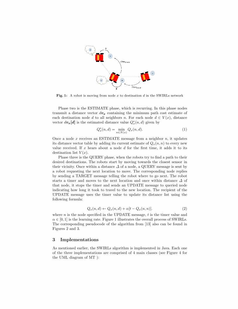
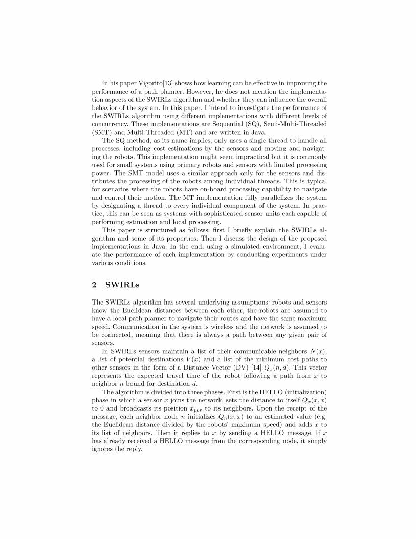
Fig. 1: A robot is moving from node x to destination d in the SWIRLs network

Phase two is the ESTIMATE phase, which is recurring. In this phase nodestransmit a distance vector dvx containing the minimum path cost estimate ofeach destination node d to all neighbors n. For each node d ∈ V (x), distancevector dvx[d] is the estimated distance value Q∗x(n, d) given by

Q∗x(n, d) = minn∈N(x)

Qx(n, d). (1)

Once a node x receives an ESTIMATE message from a neighbor n, it updatesits distance vector table by adding its current estimate of Qx(n, n) to every newvalue received. If x hears about a node d for the first time, it adds it to itsdestination list V (x).

Phase three is the QUERY phase, when the robots try to find a path to theirdesired destinations. The robots start by moving towards the closest sensor intheir vicinity. Once within a distance ∆ of a node, a QUERY message is sent bya robot requesting the next location to move. The corresponding node repliesby sending a TARGET message telling the robot where to go next. The robotstarts a timer and moves to the next location and once within distance ∆ ofthat node, it stops the timer and sends an UPDATE message to queried nodeindicating how long it took to travel to the new location. The recipient of theUPDATE message uses the timer value to update its distance list using thefollowing formula:

Qx(n, d)← Qx(n, d) + α[t−Qx(n, n)]. (2)

where n is the node specified in the UPDATE message, t is the timer value andα ∈ [0, 1] is the learning rate. Figure 1 illustrates the overall process of SWIRLs.The corresponding pseudocode of the algorithm from [13] also can be found inFigures 2 and 3.

3 Implementations

As mentioned earlier, the SWIRLs algorithm is implemented in Java. Each oneof the three implementations are comprised of 4 main classes (see Figure 4 forthe UML diagram of MT ):

d← destination nodecurrent← nullnext← closest neighboring nodewhile (distance to d > ∆) :restart timerwhile(distance to next > ∆) :move towards next using local navigation

endif(current ! = null) :send UPDATE(next, timer) to current

endifsendQUERY (d) to next andwait for TARGET (n)current← nextnext← nend

Fig. 2: Pseudocode for robots

1. Robot class: this class simulates the behavior of a robot and includes meth-ods such as timer() to measure travel cost between two sensors, sendQuery()to communicate with sensors and move() to move the robot from one pointto another.

2. Sensor class: this class behaves as a sensor and includes methods such asinitialize() and estimate() to perform updates, and query() and receive()to handle communications with robots and sensors.

3. Message class: this class forms different types of messages. Depending onthe type of constructor used, it can be a HELLO, ESTIMATE, QUERY,TARGET or UPDATE message.

4. Controller class: this is the main class, which plays a different role depend-ing on the type of implementation, including initialization of the system,handling communications and control.

3.1 Sequential Implementation

The Controller object in the Sequential (SQ) implementation is responsible forthe entire operation. Its tasks include generating and initializing sensors androbots objects, and handling all communications between them. The calcula-tions, such as distance estimation, target selection and message generation aredone locally in the Sensor and Robot classes. The SQ method only uses a singlethread to process all tasks, which means every time a component is in process,the entire system is halted.

The messages are passed between components using two List < Message >structures. In each cycle the Controller reads the messages one by one, identifiesthe recipient of each one and sends them to the corresponding parties. The tar-gets proposed by the sensors are placed in a Map < Character, Message > withthe Key corresponding to the robot’s id and the Value containing the message.

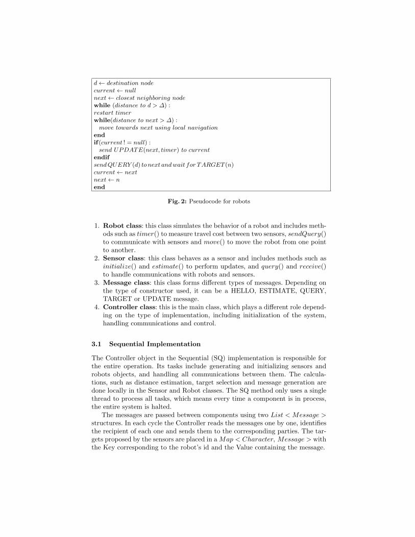
InitializeQx(x, x)← 0broadcastHELLO(xpos)loop forever:process any receivedmessagesmusing receive(m)compute distance vector dvx according to dvx[d] ← minn∈N(x)Qx(n, d), ∀d ∈ V (x)broadcastESTIMATE(dvx)

endreceive(m)if(misHELLO(npos)&&n /∈ N(x)) :N(x)← n ∪N(x)initializeQx(n, n) optimistically based onnpos

sendHELLO(xpos) to nendifif(misESTIMATE(dvn)) :Qx(n, d)← dvn[d]+Qx(n, n), ∀d ∈ dvn

if(d /∈ V (x)) : V (x)← d ∪ V (x),∀d ∈ dvnendifendifif(misQUERY (d)) :sendTARGET (arg minn∈N(x)Qx(n, d) to querying robot

endifif(misUPDATE(n, timer)) :Qx(n, d)← Qx(n, d) + α[timer −Qx(n, n)], ∀d ∈ V (x)endifend

Fig. 3: Pseudocode for sensors

3.2 Semi-Multi-Threaded Implementation

The Semi-Multi-Threaded (SMT) model is similar to SQ with the differencethat the Controller object only handles communications between the sensors,and transmits the robots messages to them. The robots, on the other hand, arerun on a separate thread and communicate with Controller through a shared datastructure, BlockingQueue < Message >. To access the elements of the queueoffer() and poll() methods are used to avoid unnecessary blocking in the system.The TARGET messages for the robots are transmitted using ConcurrentMap <Message >, which manages the synchronization internally when necessary.

In special circumstances, when a sensor is not aware of a requested destina-tion, the Controller creates a list of the rejected queries made by the robots. Ineach round of the program the messages in the reject list are re-transmitted tothe sensors. In such cases, the requesting robot stays idle until it receives a validtarget from the corresponding sensor.

3.3 Multi-Threaded Implementation

The Multi-Threaded (MT) implementation is fully concurrent, i.e. all the compo-nents of the system are run on separate threads. The communications in the sys-tem is handled using 4 data structures of typeMap < Integer,BlockingQueue <

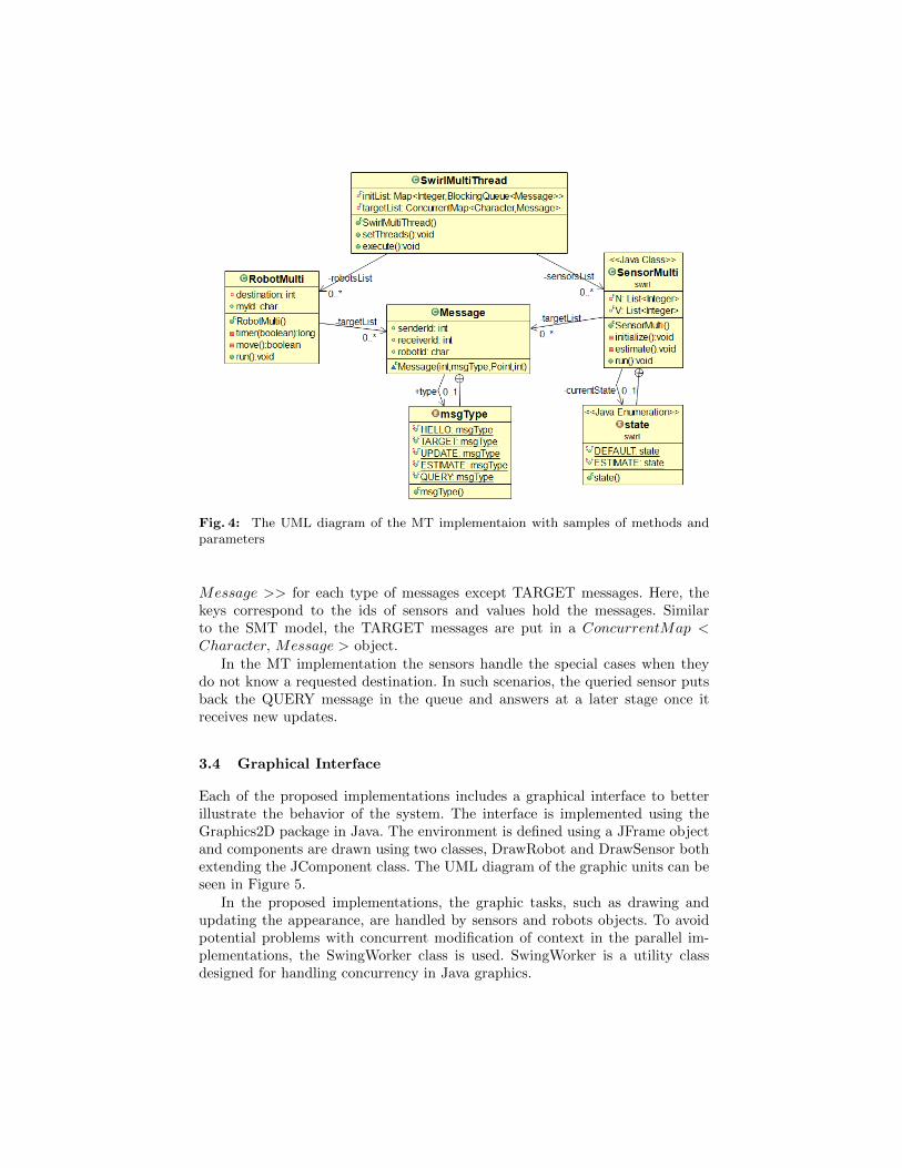
Fig. 4: The UML diagram of the MT implementaion with samples of methods andparameters

Message >> for each type of messages except TARGET messages. Here, thekeys correspond to the ids of sensors and values hold the messages. Similarto the SMT model, the TARGET messages are put in a ConcurrentMap <Character, Message > object.

In the MT implementation the sensors handle the special cases when theydo not know a requested destination. In such scenarios, the queried sensor putsback the QUERY message in the queue and answers at a later stage once itreceives new updates.

3.4 Graphical Interface

Each of the proposed implementations includes a graphical interface to betterillustrate the behavior of the system. The interface is implemented using theGraphics2D package in Java. The environment is defined using a JFrame objectand components are drawn using two classes, DrawRobot and DrawSensor bothextending the JComponent class. The UML diagram of the graphic units can beseen in Figure 5.

In the proposed implementations, the graphic tasks, such as drawing andupdating the appearance, are handled by sensors and robots objects. To avoidpotential problems with concurrent modification of context in the parallel im-plementations, the SwingWorker class is used. SwingWorker is a utility classdesigned for handling concurrency in Java graphics.

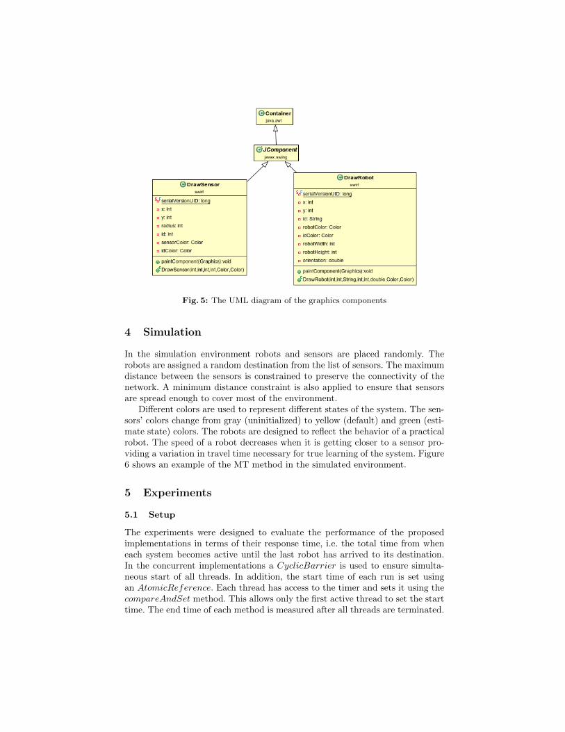
Fig. 5: The UML diagram of the graphics components

4 Simulation

In the simulation environment robots and sensors are placed randomly. Therobots are assigned a random destination from the list of sensors. The maximumdistance between the sensors is constrained to preserve the connectivity of thenetwork. A minimum distance constraint is also applied to ensure that sensorsare spread enough to cover most of the environment.

Different colors are used to represent different states of the system. The sen-sors’ colors change from gray (uninitialized) to yellow (default) and green (esti-mate state) colors. The robots are designed to reflect the behavior of a practicalrobot. The speed of a robot decreases when it is getting closer to a sensor pro-viding a variation in travel time necessary for true learning of the system. Figure6 shows an example of the MT method in the simulated environment.

5 Experiments

5.1 Setup

The experiments were designed to evaluate the performance of the proposedimplementations in terms of their response time, i.e. the total time from wheneach system becomes active until the last robot has arrived to its destination.In the concurrent implementations a CyclicBarrier is used to ensure simulta-neous start of all threads. In addition, the start time of each run is set usingan AtomicReference. Each thread has access to the timer and sets it using thecompareAndSet method. This allows only the first active thread to set the starttime. The end time of each method is measured after all threads are terminated.

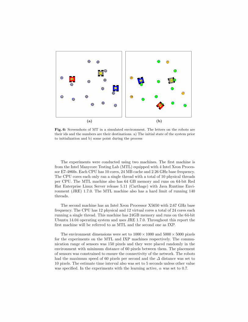
(a) (b)

Fig. 6: Screenshots of MT in a simulated environment. The letters on the robots aretheir ids and the numbers are their destinations. a) The initial state of the system priorto initialization and b) some point during the process

The experiments were conducted using two machines. The first machine isfrom the Intel Manycore Testing Lab (MTL) equipped with 4 Intel Xeon Proces-sor E7-4860s. Each CPU has 10 cores, 24 MB cache and 2.26 GHz base frequency.The CPU cores each only ran a single thread with a total of 10 physical threadsper CPU. The MTL machine also has 64 GB memory and runs on 64-bit RedHat Enterprise Linux Server release 5.11 (Carthage) with Java Runtime Envi-ronment (JRE) 1.7.0. The MTL machine also has a hard limit of running 140threads.

The second machine has an Intel Xeon Processor X5650 with 2.67 GHz basefrequency. The CPU has 12 physical and 12 virtual cores a total of 24 cores eachrunning a single thread. This machine has 24GB memory and runs on the 64-bitUbuntu 14.04 operating system and uses JRE 1.7.0. Throughout this report thefirst machine will be referred to as MTL and the second one as IXP.

The environment dimensions were set to 1000× 1000 and 5000× 5000 pixelsfor the experiments on the MTL and IXP machines respectively. The commu-nication range of sensors was 150 pixels and they were placed randomly in theenvironment with minimum distance of 60 pixels between them. The placementof sensors was constrained to ensure the connectivity of the network. The robotshad the maximum speed of 60 pixels per second and the ∆ distance was set to10 pixels. The estimate time interval also was set to 5 seconds unless other valuewas specified. In the experiments with the learning active, α was set to 0.7.

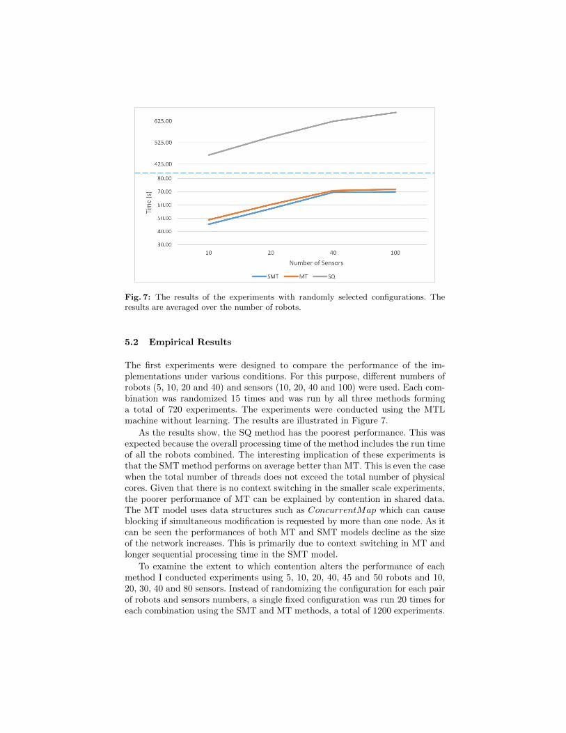
Fig. 7: The results of the experiments with randomly selected configurations. Theresults are averaged over the number of robots.

5.2 Empirical Results

The first experiments were designed to compare the performance of the im-plementations under various conditions. For this purpose, different numbers ofrobots (5, 10, 20 and 40) and sensors (10, 20, 40 and 100) were used. Each com-bination was randomized 15 times and was run by all three methods forminga total of 720 experiments. The experiments were conducted using the MTLmachine without learning. The results are illustrated in Figure 7.

As the results show, the SQ method has the poorest performance. This wasexpected because the overall processing time of the method includes the run timeof all the robots combined. The interesting implication of these experiments isthat the SMT method performs on average better than MT. This is even the casewhen the total number of threads does not exceed the total number of physicalcores. Given that there is no context switching in the smaller scale experiments,the poorer performance of MT can be explained by contention in shared data.The MT model uses data structures such as ConcurrentMap which can causeblocking if simultaneous modification is requested by more than one node. As itcan be seen the performances of both MT and SMT models decline as the sizeof the network increases. This is primarily due to context switching in MT andlonger sequential processing time in the SMT model.

To examine the extent to which contention alters the performance of eachmethod I conducted experiments using 5, 10, 20, 40, 45 and 50 robots and 10,20, 30, 40 and 80 sensors. Instead of randomizing the configuration for each pairof robots and sensors numbers, a single fixed configuration was run 20 times foreach combination using the SMT and MT methods, a total of 1200 experiments.

(a)

(b)

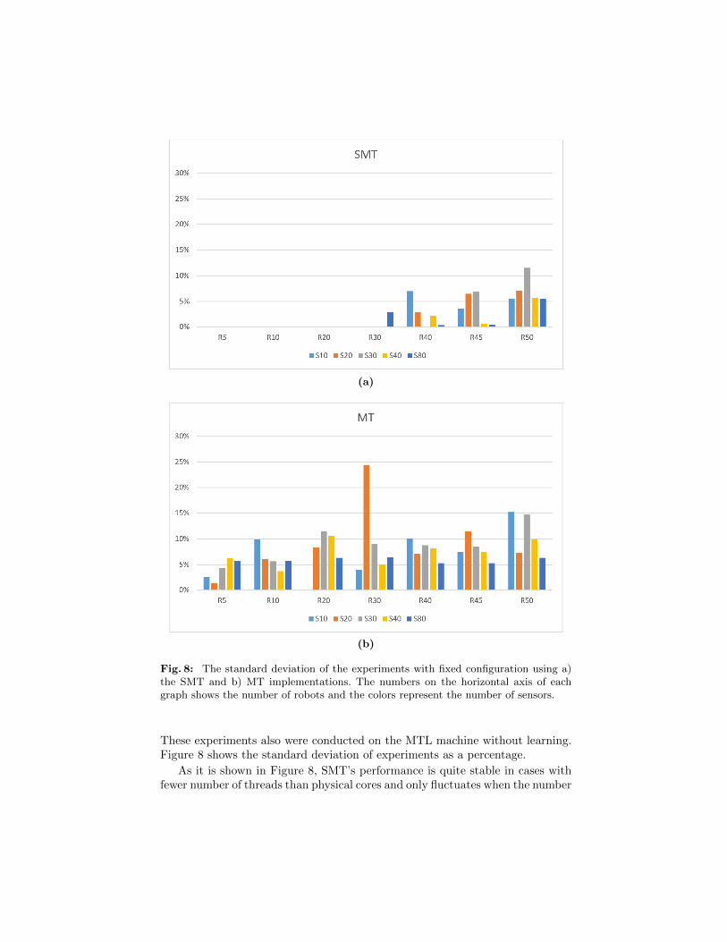
Fig. 8: The standard deviation of the experiments with fixed configuration using a)the SMT and b) MT implementations. The numbers on the horizontal axis of eachgraph shows the number of robots and the colors represent the number of sensors.

These experiments also were conducted on the MTL machine without learning.Figure 8 shows the standard deviation of experiments as a percentage.

As it is shown in Figure 8, SMT’s performance is quite stable in cases withfewer number of threads than physical cores and only fluctuates when the number

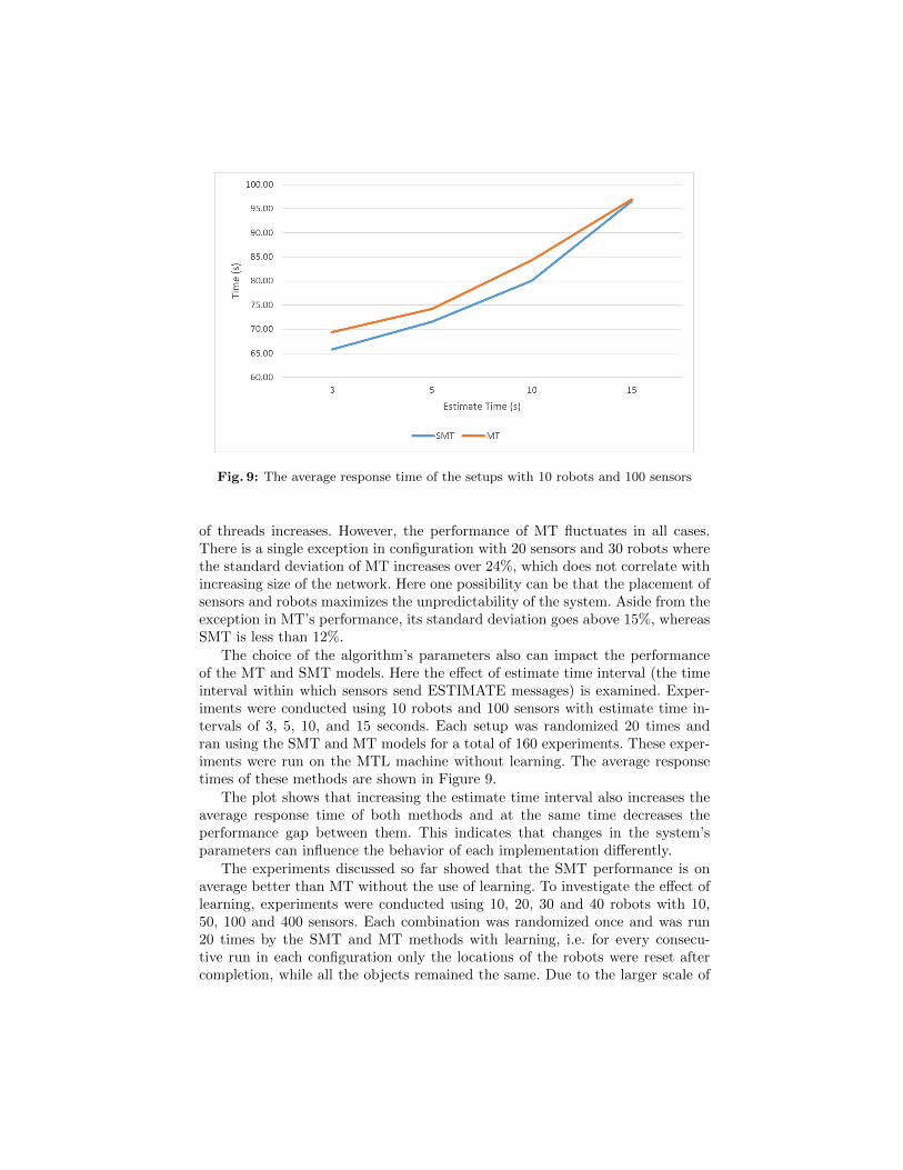
Fig. 9: The average response time of the setups with 10 robots and 100 sensors

of threads increases. However, the performance of MT fluctuates in all cases.There is a single exception in configuration with 20 sensors and 30 robots wherethe standard deviation of MT increases over 24%, which does not correlate withincreasing size of the network. Here one possibility can be that the placement ofsensors and robots maximizes the unpredictability of the system. Aside from theexception in MT’s performance, its standard deviation goes above 15%, whereasSMT is less than 12%.

The choice of the algorithm’s parameters also can impact the performanceof the MT and SMT models. Here the effect of estimate time interval (the timeinterval within which sensors send ESTIMATE messages) is examined. Exper-iments were conducted using 10 robots and 100 sensors with estimate time in-tervals of 3, 5, 10, and 15 seconds. Each setup was randomized 20 times andran using the SMT and MT models for a total of 160 experiments. These exper-iments were run on the MTL machine without learning. The average responsetimes of these methods are shown in Figure 9.

The plot shows that increasing the estimate time interval also increases theaverage response time of both methods and at the same time decreases theperformance gap between them. This indicates that changes in the system’sparameters can influence the behavior of each implementation differently.

The experiments discussed so far showed that the SMT performance is onaverage better than MT without the use of learning. To investigate the effect oflearning, experiments were conducted using 10, 20, 30 and 40 robots with 10,50, 100 and 400 sensors. Each combination was randomized once and was run20 times by the SMT and MT methods with learning, i.e. for every consecu-tive run in each configuration only the locations of the robots were reset aftercompletion, while all the objects remained the same. Due to the larger scale of

Fig. 10: The average result of the experiments with active learning over 20 trials

these experiments they were conducted on the IXP machine. The average resultof each run is reflected in Figure 10.

As expected, in the first run where no learning has taken place, the SMTmethod performed better than MT. However, from the second trial onward,the MT implementation learns much faster in comparison to SMT and performsbetter. The MT method reaches its best performance after the third run, whereasit takes SMT to achieve a similar level of performance after 7 runs. Despite MThas a faster learning rate, in the long run both models still perform similarlywith more stable behavior by SMT, as was shown earlier.

Finally, I investigated whether for any size of the network the sequentialcomputation of the SMT model becomes computationally more expensive thancontention and context switching in MT. For this purpose, experiments wereconducted on a larger scale using the IXP machine with 4 robots and 20, 40, 80,160, 320, 640 and 1280 sensors. Each configuration was randomized once andwas run 20 times with learning for each implementation, forming a total of 420experiments. Figure 11 shows the average response time of the implementationsin each configuration.

The results show that as the number of sensors increases beyond 640, theperformance gap between MT and SMT increases significantly. At this point,the performance of the SMT model exponentially declines getting closer to theSQ model.

6 Conclusion

In this paper three implementations of a physical path planning algorithm knownas Swarm of Interacting Reinforcement Learners (SWIRLs) was presented. The

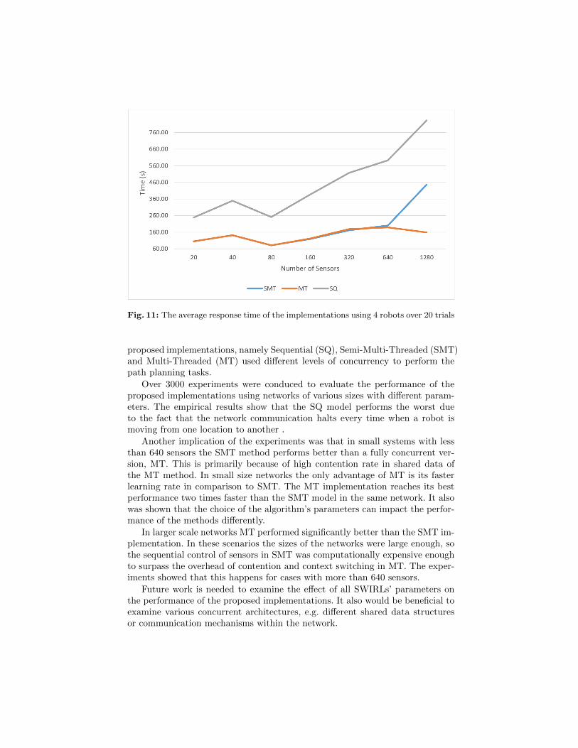
Fig. 11: The average response time of the implementations using 4 robots over 20 trials

proposed implementations, namely Sequential (SQ), Semi-Multi-Threaded (SMT)and Multi-Threaded (MT) used different levels of concurrency to perform thepath planning tasks.

Over 3000 experiments were conduced to evaluate the performance of theproposed implementations using networks of various sizes with different param-eters. The empirical results show that the SQ model performs the worst dueto the fact that the network communication halts every time when a robot ismoving from one location to another .

Another implication of the experiments was that in small systems with lessthan 640 sensors the SMT method performs better than a fully concurrent ver-sion, MT. This is primarily because of high contention rate in shared data ofthe MT method. In small size networks the only advantage of MT is its fasterlearning rate in comparison to SMT. The MT implementation reaches its bestperformance two times faster than the SMT model in the same network. It alsowas shown that the choice of the algorithm’s parameters can impact the perfor-mance of the methods differently.

In larger scale networks MT performed significantly better than the SMT im-plementation. In these scenarios the sizes of the networks were large enough, sothe sequential control of sensors in SMT was computationally expensive enoughto surpass the overhead of contention and context switching in MT. The exper-iments showed that this happens for cases with more than 640 sensors.

Future work is needed to examine the effect of all SWIRLs’ parameters onthe performance of the proposed implementations. It also would be beneficial toexamine various concurrent architectures, e.g. different shared data structuresor communication mechanisms within the network.

Acknowledgements. Thanks to the management, staff, and facilities of theIntel Manycore Testing Lab.Home: http://www.intel.com/software/manycoretestinglab.Intel Software Network: http://www.intel.com/software.

References

1. Brooks, R.: A robust layered control system for a mobile robot. InternationalJournal of Robotics and Automation 2(1) (March 1986) 14–23

2. Koryakovski, I., Hoai, N.X., Lee, K.M.: A genetic algorithm with local map forpath planning in dynamic environments. In: Proceedings of 11th Annual conferenceon Genetic and evolutionary computation, Montreal (July 2009) 1859–1860

3. Ferguson, D., Stentz, A.: The field d* algorithm for improved path planning andreplanning in uniform and non-uniform cost environments. Technical Report CMU-RI-TR-05-19,, Robotics Institute, Carnegie Mellon University (June 2005)

4. Fox, D.: Markov localization: A Probabilistic Framework for Mobile Robot Local-ization and Navigation. PhD thesis, Institute of Computer Science III, Universityof Bonn (1998)

5. Konidaris, G.D., Hayes, G.M.: An architecture for behavior-based reinforcementlearning. Journal of Adaptive Behavior 13(1) (March 2005) 5–32

6. Agmon, N.: On events in multi-robot patrol in adversarial environments. In:Proceedings of the 9th International Conference on Autonomous Agents and Mul-tiagent Systems. Volume 2., Toronto (May 2010) 591–598

7. Vokrinek, J., Komenda, A., Pechoucek, M.: Cooperative agent navigation in par-tially unknown urban environments. In: Proceedings of the 3rd International Sym-posium on Practical Cognitive Agents and Robots, Toronto (May 2010) 41–48

8. O’Hara, K.J., Bigio, V., Whitt, S., Walker, D., Balch, T.: Evaluation of a largescale pervasive embedded network for robot path planning. In: Proceedings ofIEEE International Conference on Robotics and Automation (ICRA 06), Orlando(April 2006)

9. Batalin, M.A., Sukhatme, G.S., Hattig, M.: Mobile robot navigation using a sen-sor network. In: Proceedings of IEEE International Conference on Robotics andAutomation (ICRA 04), New Orlean (April 2004) 636–642

10. Li, Q., DeRosa, M., D., R.: Distributed algorithms for guiding navigation across asensor network. In: Proceedings of 9th International Conference on Mobile Com-puting and Networking, San Diego (September 2003) 313–325

11. Banerjee, S., Detweiler, C.: Path planning algorithms for robotic underwater sens-ing in a network of sensors. In: Proceedings of the International Conference onUnderwater Networks & Systems, Rome (November 2014)

12. Lambrou, T.P.: Optimized cooperative dynamic coverage in mixed sensor networks.ACM Transactions on Sensor Networks 11(3) (May 2015)

13. Vigorito, C.M.: Distributed path planning for mobile robots using a swarm ofinteracting reinforcement learners. In: Proceedings of the 6th international jointconference on Autonomous agents and multiagent systems, Honolulu (May 2007)

14. Royer, E.M., K., T.C.: A review of current routing protocols for ad-hoc mobilewireless networks. Journal IEEE Personal Communications (April 1999) 46–55