SWARM KEEPING STRATEGIES FOR SPACECRAFTUNDER J2 AND ATMOSPHERIC DRAG PERTURBATIONS

BY

DANIEL JAMES MORGAN

THESIS

Submitted in partial fulfillment of the requirementsfor the degree of Master of Science in Aerospace Engineering

in the Graduate College of theUniversity of Illinois at Urbana-Champaign, 2011

Urbana, Illinois

Adviser:

Assistant Professor Soon-Jo Chung

Abstract

This thesis presents several new open-loop guidance methods for spacecraft swarms

comprised of hundreds to thousands of agents with each spacecraft having modest

capabilities. These methods have three main goals: preventing relative drift of the

swarm, preventing collisions within the swarm, and minimizing the fuel used through-

out the mission. The development of these methods progresses by eliminating drift

using the Hill-Clohessy-Wiltshire equations, removing drift due to nonlinearity, and

minimizing the J2 drift. In order to verify these guidance methods, a new dynamic

model for the relative motion of spacecraft is developed. These dynamics are exact

and include the two main disturbances for spacecraft in Low Earth Orbit (LEO), J2

and atmospheric drag. Using this dynamic model, numerical simulations are provided

at each step to show the effectiveness of each method and to see where improvements

can be made. The main result is a set of initial conditions for each spacecraft in the

swarm which provides hundreds of collision-free orbits in the presence of J2. Finally,

a multi-burn strategy is developed in order to provide hundreds of collision free orbits

under the influence of atmospheric drag. This last method works by enforcing the

initial conditions multiple times throughout the mission thereby providing collision

free motion for the duration of the mission.

ii

Acknowledgments

The author wishes to thank Dr. Soon-Jo Chung for the opportunity to work on

this project and for his guidance on this research. Special thanks to Dr. Fred Y.

Hadaegh of NASA Jet Propulsion Laboratory for his guidance and support on this

project. Additional thanks to Dr. Lars Blackmore, Dr. Behcet Acikmese, and Dr.

David Bayard of NASA Jet Propulsion Laboratory for their constructive comments.

Also, thanks to Insu Chang and Austin Nicholas for their help with simulations and

insightful discussions. Finally, thanks to my girlfriend and family for their support

during the process of earning my Master’s Degree.

iii

Table of Contents

Nomenclature . . . . . . . . . . . . . . . . . . . . . . . . . . . . . . . . . v

1 Introduction . . . . . . . . . . . . . . . . . . . . . . . . . . . . . . . . 1

2 Swarm Initialization . . . . . . . . . . . . . . . . . . . . . . . . . . . 6

3 Exact Dynamics with J2 and Drag . . . . . . . . . . . . . . . . . . 10

4 Single Burn Swarm Keeping Options . . . . . . . . . . . . . . . . . 17

5 Swarm Keeping Methods for J2 PerturbedOrbits . . . . . . . . . . . . . . . . . . . . . . . . . . . . . . . . . . . 28

6 Swarm Keeping for J2 and Atmospheric Drag Perturbed Orbits . 40

7 Conclusion . . . . . . . . . . . . . . . . . . . . . . . . . . . . . . . . . 45

References . . . . . . . . . . . . . . . . . . . . . . . . . . . . . . . . . . . 47

iv

Nomenclature

A cross sectional area of chief spacecraft

Cd drag coefficient

CF collision fraction

D drift of spacecraft

D average drift of swarm

~F drag force on chief spacecraft

J2 second harmonic coefficient of Earth

N(ν, σ) Normal distribution with mean ν and standard deviation σ

Qn generalized force corresponding to qn

Re radius of the Earth

~V velocity of chief spacecraft

~Va velocity of chief spacecraft relative to atmosphere

X collision distance

(X, Y , Z) ECI coordinate system

~adrag drag acceleration vector

h angular momentum

i orbit inclination

kJ232J2µR

2e, 2.633× 1010 [km5/s2]

~l relative position vector

~l relative velocity vector

m mass of spacecraft

n number of spacecraft

qn generalized coordinate

r geocentric distance

v

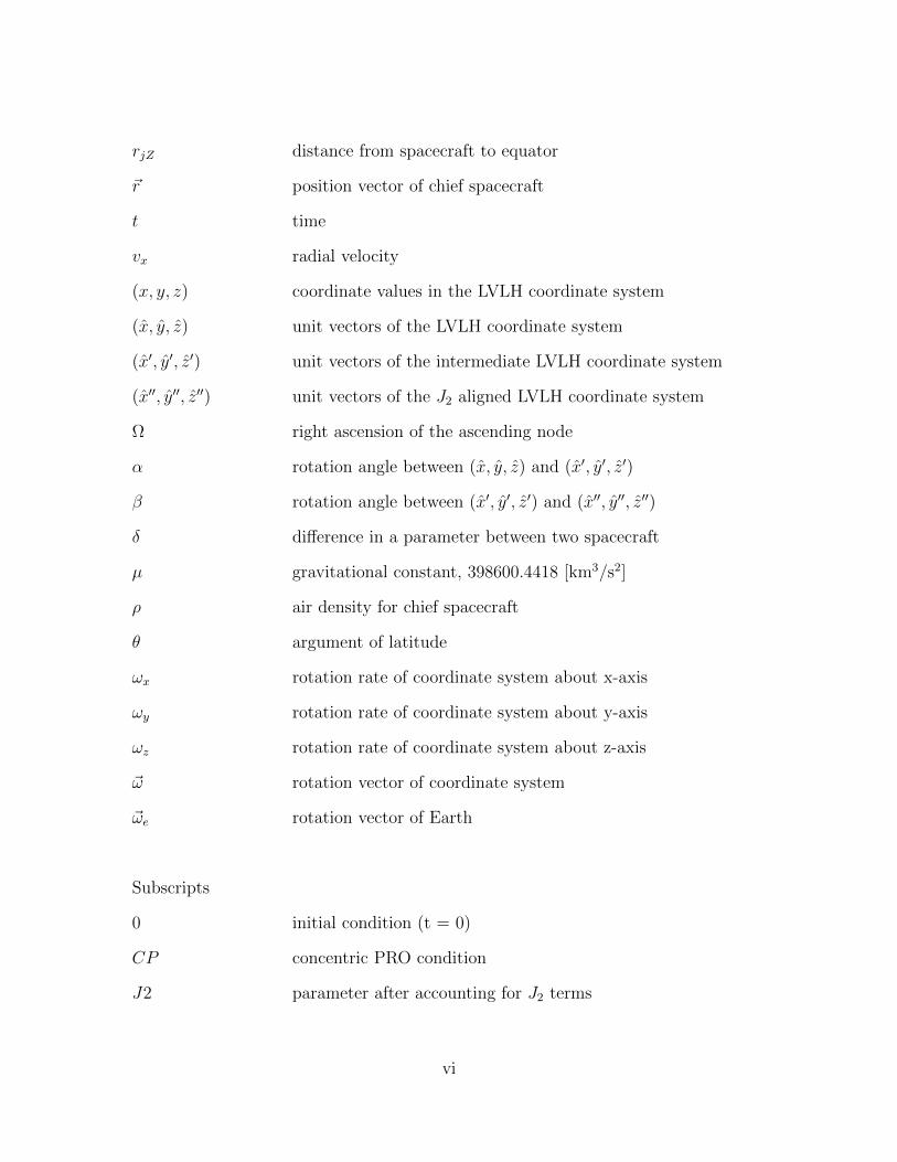
rjZ distance from spacecraft to equator

~r position vector of chief spacecraft

t time

vx radial velocity

(x, y, z) coordinate values in the LVLH coordinate system

(x, y, z) unit vectors of the LVLH coordinate system

(x′, y′, z′) unit vectors of the intermediate LVLH coordinate system

(x′′, y′′, z′′) unit vectors of the J2 aligned LVLH coordinate system

Ω right ascension of the ascending node

α rotation angle between (x, y, z) and (x′, y′, z′)

β rotation angle between (x′, y′, z′) and (x′′, y′′, z′′)

δ difference in a parameter between two spacecraft

µ gravitational constant, 398600.4418 [km3/s2]

ρ air density for chief spacecraft

θ argument of latitude

ωx rotation rate of coordinate system about x-axis

ωy rotation rate of coordinate system about y-axis

ωz rotation rate of coordinate system about z-axis

~ω rotation vector of coordinate system

~ωe rotation vector of Earth

Subscripts

0 initial condition (t = 0)

CP concentric PRO condition

J2 parameter after accounting for J2 terms

vi

L linearized condition

N nonlinear condition (main result)

PM period matched condition

j parameter of deputy spacecraft (j ≤ n)

r desired condition of deputy spacecraft

vii

1 Introduction

Formation flying spacecraft have been a major area of research over the past decade

due to their ability to perform certain tasks, such as interferometry [1] and distributed

sensing [2], and their potential to achieve performance at a cheaper cost than mono-

lithic spacecraft. An expensive monolithic spacecraft can be replaced by many low

cost spacecraft. Another advantage of formation flying (FF) spacecraft is that the

formation as a whole is more redundant than a monolithic spacecraft because the

failure of a single spacecraft in the formation can be overcome by the rest of the

formation whereas the failure of a monolithic spacecraft most likely results in the

failure of the mission. One of the main challenges of FF spacecraft is the Guidance,

Navigation, and Control (GN&C) of the formation. As a result, a substantial amount

of research has been done on the GN&C of FF spacecraft [3, 4, 5, 6, 7, 8, 9, 10, 11]

in the last decade.

This thesis is concerned with the GN&C of a challenging type of formation flying,

spacecraft swarms. A swarm is defined as a collection of 1000 or more spacecraft

with masses on the order of 100g [12]. These swarms have potential for use as optical

relays, distributed antennas, or for massively distributed sensing applications among

others. Ongoing research in microfabrication is developing the technologies required

to fabricate, at low cost-per-unit, a 100g class of spacecraft, called femtosats, that

can be actively controlled in all six degrees of freedom [12].

The large increase in the number of spacecraft (two orders of magnitude larger

than typical FF) and the small size of each spacecraft create several key challenges in

spacecraft swarm control. The main challenge is the large increase in the probability

of collisions caused by having so many spacecraft in such a small volume. Addi-

tionally, fuel efficiency becomes much more important because the size of the each

1

spacecraft will limit the amount of fuel that can be carried by each spacecraft. One

way to eliminate the need for complex controllers is to use J2 invariant relative orbits,

where the relative distance between spacecraft will be constant, thereby dramatically

reducing the possibility of collisions. Another benefit of J2 invariant relative orbits

is that they are more fuel efficient than other orbits because they do not require cor-

rections to account for J2 drift. Even when J2 drift is eliminated, atmospheric drag

will cause the spacecraft to drift apart. One of the biggest problems when accounting

for these perturbations, especially atmospheric drag, is the lack of an exact relative

dynamic model including perturbations.

There are many dynamic models in the literature but each of them has limitations.

For spacecraft separations on the order of hundreds of meters, the Hill-Clohessy-

Wiltshire (HCW) equations have been shown to be good linear approximations of

the relative dynamics [13], with the added advantage that the resulting linear time

invariant system has a closed form solution. In addition to assuming small separations

from the reference orbit, the HCW equations also assume a circular reference orbit

around a perfectly spherical, and homogeneous Earth. These assumptions can lead to

large errors in the motion predicted by the HCW equations. There have been many

attempts to develop more exact dynamics by removing some of the assumptions made

in the HCW equations. Tschauner and Hempel [14] removed the restriction of circular

orbits and developed the linear equations of motion for any orbit around a spherical

Earth. Schweigart and Sedwick [15] developed linearized dynamics which include J2

effects and Hamel and Lafontaine [16] extended this work to include eccentric orbits.

Although these dynamic models are more accurate than the HCW equations, the

linearization of the dynamics induces large errors when spacecraft separations are

large. The relative dynamics have also been derived in the form of a state transition

matrix [17]. If the initial states of an orbit are known, the state transition matrix can

2

be used to find the states at any given time. The main drawback of this approach is

that the state transition matrix has a complicated form, which makes it difficult to

use. Exact nonlinear dynamics, which include the J2 perturbation, were developed

by Xu and Wang [18]. Chang et al. [19] derived an exact nonlinear dynamic model

which includes both J2 and atmospheric drag. However, the dynamics for the chief

use classical orbital elements, which might make the implementation of the dynamic

model more complicated. Therefore, this paper takes the method used by Xu and

Wang [18] and extends it to include atmospheric drag in addition to J2 effects using

hybrid orbital elements. This produces an exact dynamic model which includes the

major perturbations experienced by spacecraft in LEO. The derivation of this dynamic

model can be found in Section 3.

Several papers have attempted to find J2 invariant relative motion between two

spacecraft. The most popular method for finding these orbits is to set the differen-

tial mean orbital elements equal to zero using Gauss’s variational equations (GVEs)

to propagate the change in each spacecraft’s orbital elements [6, 7, 8, 9]. Breger et

al. [10] found partial J2 invariant orbits using the state transition matrix [17] and op-

timized the motion for minimum drift and fuel. Then, Breger and How [11] developed

new linear time varying relative equations of motion and applied an online, model

predictive controller to these dynamics. The methods developed by using GVEs and

mean orbital elements are limited by the fact that they are designed for formations

of ten or fewer spacecraft; however, the number of spacecraft in a swarm as well as

the limited capability of each spacecraft creates several problems, which these con-

trollers were not designed to handle. Mainly, the number of possible collisions scales

quadratically with the number of spacecraft so in a swarm of thousands of spacecraft

there are hundreds of thousands of possible collisions. This makes path planning and

control a much more difficult problem.

3

In this paper, swarm keeping means maintaining relative distances between mul-

tiple spacecraft in the presence of disturbances and ensuring that collisions do not

occur. The swarm keeping methods considered in this paper are motivated by four in-

creasingly more realistic and complex dynamic models: (i) linearized dynamics given

by the HCW equations, (ii) Keplerian dynamics with spherical Earth assumptions,

(iii) exact dynamics with J2 [18], and (iv) exact dynamics with J2 and atmospheric

drag (derived in Section 3). Furthermore, regardless of which model is used to mo-

tivate the swarm keeping method, each method is evaluated using dynamic models

(ii) and (iii), except in Section 6 where atmospheric drag is considered and dynamic

model (iv) is used.

The main contribution of this paper is the investigation of various methods of

swarm keeping and using numerical simulations to show the effectiveness of each

method. Energy matching conditions are introduced in Section 5 as a method for

swarm keeping with respect to J2 influence [20]. Energy matching is shown by simu-

lation, in the presence of J2, to provide collision free swarm motion for several hundred

orbits with only a single initializing burn by each agent. Related work has found other

conditions that prove J2 invariance under certain restricted orbits [6, 7, 8, 9, 10]. In

comparison, simulations in Section 5 suggest that energy matching provides a pow-

erful method to minimize both swarm drift rate and the collision rate across a wide

range of reference orbits regardless of altitude, eccentricity, and inclination. A main

contribution of this paper is to identify energy matching as a very effective approach

to swarm keeping. In Section 6, a multi-burn guidance method is developed and

implemented which extends the energy matching method so that it is effective in

the presence of atmospheric drag in addition to J2. The collision free equations and

multi-burn guidance method are designed specifically to address the major concerns

of spacecraft swarm GN&C, including collision avoidance and fuel efficiency.

4

The paper is organized as follows. The problem statement and the assumptions

made in initializing the swarm are described in Section 2. Additionally, the metrics

that are used to quantify the swarm motion are defined. In Section 3, an exact dy-

namic model is developed, which includes the effects of both J2 and atmospheric drag.

In Section 4, the effect of J2 on the swarm is investigated and the HCW equations

are used to develop some simple single burn control options. In Section 5, the main

results are presented by expanding upon the equations developed in Section 4 taking

into account the J2 perturbation. In Section 6, the effects of atmospheric drag are

investigated and a multi-burn guidance method based on the equations developed in

Section 5 is used in order to provide collision free motion in an environment perturbed

by both J2 and drag.

5

2 Swarm Initialization

In order to derive the relative dynamics, two coordinate systems must be defined.

First, the Earth Centered Inertial (ECI) coordinate system is used to locate the chief

spacecraft or a virtual reference point called the chief orbit (see Fig. 1a). This coor-

dinate system is fixed and located at the center of the Earth. The X direction points

towards the vernal equinox, the Z direction points towards the north pole, and the Y

direction is perpendicular to the other two and completes the right-handed coordinate

system. The second coordinate system is the Local Vertical, Local Horizonal (LVLH)

coordinate system. The LVLH frame is centered at the chief spacecraft or chief orbit.

Figure 1a shows the LVLH frame with respect to a chief spacecraft. The x, or radial,

direction is always aligned with the position vector and points away from the Earth,

the z, or crosstrack, direction is aligned with the angular momentum vector, and the

y, or alongtrack, direction completes the right-handed coordinate system. The LVLH

frame is a rotating frame with a rotation rate of ωx about the radial axis and ωz

about the crosstrack axis. In other words, ωx is the precession rate of the coordinate

system and ωz is the orbital rotation rate.

The chief orbit is defined using hybrid orbital elements which include: geocentric

distance (r), radial velocity (vx), angular momentum (h), inclination (i), right ascen-

sion of the ascending node (Ω), and argument of latitude (θ). These six parameters

fully define [18] the chief orbit in the ECI frame. These hybrid states are used instead

of the classical orbital elements because the orbits of the spacecraft may vary due to

the perturbations. Hybrid states still have a physical meaning when describing a

perturbed orbit. The classical orbital elements can easily be found from the hybrid

states. The exact dynamics for the chief orbit are derived in Section 3.1. Now that

the chief orbit has been located, the LVLH frame for the chief orbit can be defined and

6

Chief

Deputy

(a) ECI (X, Y , Z) and LVLH Frames (x, y, z)

Concentric PROs

(b) Spacecraft Swarm

Figure 1: A visualization of the relative coordinate system and a spacecraft swarm

used to locate the deputy spacecraft. The relative position and velocity of the deputy

spacecraft are expressed by ~lj = [ xj yj zj ]T and ~lj = [ xj yj zj ]T , respectively.

For numerical simulations in this paper, the initial distribution of the swarm is

a normal distribution in each direction. Each normal distribution is centered at the

chief, or origin of the LVLH frame, and has a standard deviation σ. In other words, the

initial position of a spacecraft can be written as (x, y, z) = (N(0, σ), N(0, σ), N(0, σ))

where all normal distributions are independent. This distribution was chosen to rep-

resent a random deployment of the swarm. The actual deployment of the spacecraft

would need to be more controlled than what is assumed for the simulations in this

paper. Therefore, the results in the following sections give conservative estimates

for the number of collisions. Additionally, each deputy has the same velocity as the

chief in the LVLH frame which means that (x, y, z) = (0, 0, 0). However, in all of

the simulations, each spacecraft performs a burn at the start of the simulation so the

assumption that all of the relative velocities are the same will not affect the swarm

motion. An example of a spacecraft swarm is shown in Fig. 1b.

Each simulation in this paper is run for a period of 500 orbits with 60 output

7

Initial Burn

Drift

Maximum

y-position

Figure 2: Drift of a Spacecraft

times per orbit. Unless otherwise specified, the nominal swarm has a circular chief

orbit with an altitude of 500 km, an inclination of 45 degrees, and an argument of

latitude of 45 degrees. The nominal swarm has 500 deputies distributed around the

chief using a standard deviation (σ) of 0.5 km.

In order to determine the effectiveness of a swarm, metrics are defined to quantify

the motion of the swarm. Two metrics are the drift of each spacecraft (Dj) and the

average drift of the swarm (D). The drift of a spacecraft is the maximum alongtrack

position in the LVLH frame over all orbits compared to the maximum alongtrack

position attained during its first orbit, and is illustrated in Fig. 2. The average drift

of the swarm is shown in the following equation.

D ,1

n

n∑j=1

Dj (1)

The collision fraction of the swarm is defined as the number of spacecraft which

have come within a distance X of another spacecraft at, or before, a given time. The

definition of collision fraction (CF ) is shown below.

8

Rj(t′) ,

0 if ‖~lj(t)−~li(t)‖ > X for all t ≤ t′ and all i 6= j

1 if ‖~lj(t)−~li(t)‖ ≤ X for any t ≤ t′ and any i 6= j

(2)

CF (t) ,1

n

n∑j=1

Rj(t) (3)

where n is the number of spacecraft, t is the time vector, and t′ is a specific time point

in t. Then, the physical collisions are defined by setting X = 1 m. It is important

to note that once a spacecraft collides, it continues on the same trajectory and can

collide with other spacecraft. However, the collision fraction measures how many of

the spacecraft have collided. Therefore, this metric is always between 0 and 1 and is

always increasing. A collision fraction of 0 means the swarm is collision free at that

time and a collision fraction of 1 means that all spacecraft have collided at least once

before that time.

9

3 Exact Dynamics with J2 and Drag

In order to accurately describe the motion of swarms of spacecraft, exact relative

dynamics in the presence of J2 and atmospheric drag are derived in this section. This

dynamic model is derived using the same method that Xu and Wang [18] used but

it is extended to include atmospheric drag terms. This model is used in Section 6 to

demonstrate the impact of atmospheric drag on the swarm motion and to verify the

effectiveness of the multi-burn guidance method.

3.1 Exact Dynamics of Reference Orbit with J2 and Drag

Proposition 1: Considering the two main disturbances in LEO, J2 gravity and

atmospheric drag, the differential equations describing the motion of the chief orbit

are as follows:

r = vx (4)

vx = − µr2

+h2

r3− kJ2

r4(1− 3 sin2 i sin2 θ)− C‖~Va‖vx (5)

h = −kJ2 sin2 i sin 2θ

r3− C‖~Va‖(h− ωer2 cos i) (6)

Ω = −2kJ2 cos i sin2 θ

hr3− C‖~Va‖ωer2 sin 2θ

2h(7)

i = −kJ2 sin 2i sin 2θ

2hr3− C‖~Va‖ωer2 sin i cos2 θ

h(8)

θ =h

r2+

2kJ2 cos2 i sin2 θ

hr3+C‖~Va‖ωer2 cos i sin 2θ

2h(9)

Proof: The rotation rate of the LVLH frame [21] is composed of the following

components:

10

ωx = i cos θ + Ω sin θ sin i (10)

ωy = −i sin θ + Ω cos θ sin i = 0 (11)

ωz = θ + Ω cos i =h

r2(12)

The motion of the chief spacecraft is determined by the following equation:

~r = −∇UJ2 + ~adrag (13)

where the gradient of the J2 perturbed gravitational potential energy (∇UJ2) is de-

fined below [18].

∇UJ2 =µ

r2x+

kJ2

r4(1− 3 sin2 i sin2 θ)x+

kJ2 sin2 i sin 2θ

r4y +

kJ2 sin 2i sin θ

r4z (14)

where µ = 398600.4418 [km3/s2] and kJ2 = 32J2µR

2e = 2.6333 × 1010 [km5/s2] are

constants for the Earth. The acceleration due to drag is

~adrag = −1

2Cd

A

mρ‖~Va‖~Va (15)

In order to simplify the drag expression, a new constant, C = 12Cd

Amρ, is defined.

The velocity of the chief spacecraft with respect to the atmosphere is found from the

following equation.

~Va = ~V − ~ωe × ~r (16)

where

11

~V = vxx+h

ry

~r = rx (17)

~ωe = ωeZ = ωe(sin θ sin ix+ cos θ sin iy + cos iz)

Evaluating Eq. (16) yields

~Va = vxx+

(h

r− ωer cos i

)y + ωer cos θ sin iz (18)

where ωe = 7.2921× 10−5 [rad/s]. Taking the second derivative of ~r yields

~r =

(vx −

h2

r3

)x+

h

ry +

ωxh

rz (19)

where vx = r, establishing Eq. (4). Evaluating the right hand side of Eq. (13) yields

−∇UJ2 + ~adrag =−[µ

r2+kJ2

r4(1− 3 sin2 i sin2 θ) + C‖~Va‖vx

]x

−[kJ2 sin2 i sin 2θ

r4+ C‖~Va‖

(h

r− ωer cos i

)]y (20)

−[kJ2 sin 2i sin θ

r4+ C‖~Va‖ωer cos θ sin i

]z

Substituting Eq. (19) and Eq. (20) into Eq. (13) establishes Eq. (5) and Eq. (6).

Additionally, the following equation for the radial rotation rate of the coordinate

system is developed.

ωx = −kJ2 sin 2i sin θ

hr3− C‖~Va‖ωer2 cos θ sin i

h(21)

Finally, solving Eqs. (10)-(12) and Eq. (21) results in Eqs. (7)-(9).

12

3.2 Exact Relative Dynamics with J2 and Drag

Proposition 2: Considering the J2 perturbation and atmospheric drag, the relative

equations of motion for the j-th spacecraft are shown below.

xj =2yjωz − xj(η2j − ω2

z) + yjαz − zjωxωz − (ζj − ζ) sin i sin θ − r(η2j − η2)

− Cj‖~Vaj‖(xj − yjωz)− (Cj‖~Vaj‖ − C‖~Va‖)vx

yj =− 2xjωz + 2zjωx − xjαz − yj(η2j − ω2

z − ω2x) + zjαx − (ζj − ζ) sin i cos θ (22)

− Cj‖~Vaj‖(yj + xjωz − zjωx)− (Cj‖~Vaj‖ − C‖~Va‖)(h

r− ωer cos i

)zj =− 2yjωx − xjωxωz − yjαx − zj(η2

j − ω2x)− (ζj − ζ) cos i

− Cj‖~Vaj‖(zj + yjωx)− (Cj‖~Vaj‖ − C‖~Va‖)ωer cos θ sin i

where η, ηj, ζ, ζj, rj, and rjZ have been introduced in order to simplify the potential

energy terms. There definitions are shown below [18].

ζ =2kJ2 sin i sin θ

r4

ζj =2kJ2rjZr5

η2 =µ

r3+kJ2

r5− 5kJ2 sin2 i sin2 θ

r5(23)

η2j =

µ

r3j

+kJ2

r5j

−5kJ2r

2jZ

r5j

rj =√

(r + xj)2 + y2j + z2

j

rjZ = (r + xj) sin i sin θ + yj sin i cos θ + zj cos i

Additionally, Cj is defined similarly to C except Cj uses the deputy values as shown

below.

13

Cj =1

2Cd,j

Ajmj

ρj (24)

The value of Cj corresponds to the j-th deputy spacecraft and each deputy will have

a different value for Cj. In general, the drag coefficient (Cd,j), the cross sectional area

(Aj), and the mass (mj) can be different for each spacecraft but in the simulations

run in this paper it is assumed that all spacecraft are the same shape and mass for

simplicity.

Proof: First, the Lagrangian (Lj) is found and substituted into Lagrange’s

equation, which is shown below.

d

dt

(∂Lj∂qn

)− ∂Lj∂qn

= Qn (25)

In this case, the qn’s are xj, yj, and zj. Now, the Lagrangian (Lj = Tj − Uj),

which is the difference between kinetic and potential energy, and the generalized

relative force in each direction (Qn) are found. The kinetic energy (per unit mass)

can be found from

Tj =1

2~Vj · ~Vj =

1

2[(vx + xj − yjωz)2 + (

h

r+ yj + xjωz − zjωx)2 + (zj + yjωx)2] (26)

where ~Vj is the velocity of the deputy spacecraft and can be found from

~Vj = (vx + xj − yjωz)x+ (h

r+ yj + xjωz − zjωx)y + (zj + yjωx)z (27)

The potential energy for the deputy spacecraft [18] (Uj) is shown below

Uj = − µrj− kJ2

r3j

(1

3−r2jZ

r2j

)(28)

14

Now, evaluating the Lagrangian yields

Lj =1

2[(vx+xj−yjωz)2+(

h

r+yj+xjωz−zjωx)2+(zj+yjωx)2]+

µ

rj+kJ2

r3j

(1

3−r2jZ

r2j

)(29)

Substituting Eq. (29) into Eq. (25) yields the exact relative dynamics for spacecraft

under the influence of J2 [18]. In order to derive a better dynamic model for spacecraft

in LEO, the effect of atmospheric drag on the relative motion is taken into account.

By including both J2 effects and drag, the dynamics derived in this paper include

both of the major perturbations experienced by spacecraft in LEO and provide more

accurate simulation results than any previous models.

Since the drag is a non-conservative force it must be found in the Qn terms. The

generalized forces will be the components of differential drag vector which is defined

below.

~Fdiff = ~Fj − ~F = −Cj‖~Vaj‖~Vaj + C‖~Va‖~Va (30)

where Cj is defined in Eq. (24) and the velocity of the deputy with respect to the

atmosphere is defined below.

~Vaj = ~Va + ~lj + ~ω ×~lj (31)

where ~lj is the relative position vector and ~lj is the relative velocity vector. The

generalized forces can be obtained from Eq. (30) as follows.

15

Qx = −Cj‖~Vaj‖(xj − yjωz)− (Cj‖~Vaj‖ − C‖~Va‖)vx (32)

Qy = −Cj‖~Vaj‖(yj + xjωz − zjωx)− (Cj‖~Vaj‖ − C‖~Va‖)(h

r− ωer cos i

)(33)

Qz = −Cj‖~Vaj‖(zj + yjωx)− (Cj‖~Vaj‖ − C‖~Va‖)ωer cos θ sin i (34)

Now all of the values required for the Lagrangian equations of motion have been

found. Substituting Eq. (29), Eq. (32), Eq. (33), and Eq. (34) into Eq. (25) re-

sults in the Lagrangian equations of motion. After much simplification, Eq. (22) is

established.

16

4 Single Burn Swarm Keeping Options

This section investigates the relative dynamics of spacecraft swarms in a J2 perturbed

orbit by allowing each spacecraft to execute a single burn at time t = 0. Since the

spacecraft are initialized with no relative velocity, the ∆V required for each burn is

equal to the velocity at t = 0+. Another way to look at this problem is that the initial

conditions for each spacecraft are set and then the exact dynamics with J2 only are

numerically integrated. For each simulation, three parameters are being investigated:

average drift (D), fuel required for the initial burn (∆V ), and collision fraction (CF ).

Average drift shows whether or not the swarm is maintaining its original shape and

how fast the swarm is dispersing, fuel required shows how expensive each option is,

and collision fraction shows how many of the spacecraft are collision free at a given

time. In an ideal scenario, all of these parameters will be small. The initial burns

discussed in the following subsections begin with the simplest, most fuel efficient

approach, and become increasingly more complex while demonstrating better drift

and collision results. The purpose of this section is to provide some simple control

methods to use as a benchmark for the main result which is developed in Section 5.

4.1 Uncontrolled Motion

Although the J2 disturbance will cause the chief orbit to drift relative to the Keplerian

orbit, it is unknown how the spacecraft will move relative to each other. For most

applications, the motion of the swarm as a whole can be perturbed as long as the

swarm itself maintains its shape. It is known that spacecraft with different orbital

periods will rapidly drift apart. In fact, running simulations for spacecraft with

different periods shows that the drift rate of the swarm is on the order of tens of

km/orbit.

17

4.2 Period Matching

4.2.1 Linearized Period Matching

In order to reduce the drift rate of the swarm, the drift caused by differences in the

orbital periods of each spacecraft is eliminated. Since the spacecraft are initialized

at a position which is within a few kilometers of the chief orbit, the HCW equations

can be used to find the initial conditions required for period matching with the only

additional constraint being a circular chief orbit. The solution to the HCW equations,

which give the relative position and velocity of the spacecraft as functions of time,

are shown below [13]:

x(t)

y(t)

z(t)

x(t)

y(t)

z(t)

=

4− 3cωzt 0 0 sωzt/ωz 2(1− cωzt)/ωz 0

6sωzt − 6ωzt 1 0 2(−1 + cωzt)/ωz 4sωzt/ωz − 3t 0

0 0 cωzt 0 0 sωzt/ωz

3ωzsωzt 0 0 cωzt 2sωzt 0

6ωz(−1 + cωzt) 0 0 −2sωzt −3 + 4cωzt 0

0 0 −ωzsωzt 0 0 cωz

x0

y0

z0

x0

y0

z0

(35)

where s(·) and c(·) represent sin(·) and cos(·), respectively.

The only terms that are secular are the ones which are multiplied by t in Eq. (35).

These terms are responsible for the majority of the drift described in Section 4.1.

Therefore, if the sum of these terms are set to zero, the drift from the previous

simulation will be reduced. Setting these terms to zero yields the conditions:

x0,L,PM = 0, y0,L,PM = −2ωzx0, z0,L,PM = 0 (36)

18

0 100 200 300 400 5000

2

4

6

8

10Average Drift vs Orbit Number

Orbit Number

Ave

rage

Drif

t (km

)

Keplerian DynamicsExact Dynamics with J

2 only

(a) Drift results

0 100 200 300 400 5000

0.2

0.4

0.6

0.8

1

Orbit Number

Fra

ctio

n of

Spa

cecr

aft C

ollid

ed

Fraction of Spacecraft Collided vs Orbit Number

Keplerian DynamicsExact Dynamics with J

2 only

(b) Collision results

Figure 3: Simulation results of a linearized period matched swarm

Since the HCW equations are used, an unperturbed circular reference orbit is assumed

and the orbital rotation rate is defined by ωz =√µ/r3.

Equation (36) are the linearized conditions required for period matching the

swarm, indicated by the subscript (L,PM). Period matching results in the second

condition in Eq. (36) and the first and third conditions are chosen in order to min-

imize fuel. Equation (36) assumes that all of the spacecraft have the zero relative

velocity upon deployment. If this is not the case, then the first and third conditions

can be modified so that the change in radial and crosstrack velocity is zero. In Sec-

tion 5, all three conditions will be fully defined, which will eliminate this dependency

on the initial velocities. The simulation results for a linearized period matched swarm

are shown in Fig. 3.

In Fig. 3a, the drift using Keplerian dynamics is nearly zero. The small drift

is caused by the fact that Eq. (35) is the linearized solution but the simulation is

run using the Keplerian dynamics, which are nonlinear. Now that the drift has been

reduced, the effect of the J2 perturbation is evident. The drift rate under exact

dynamics with J2 only is 18.4 m/orbit (over the first 500 orbits). This drift rate is

19

about 1000 times less than the drift rate in the uncontrolled swarm. At this drift

rate, the swarm size will no longer limit the swarm’s functionality.

Unfortunately, there are some disadvantages to the period matched swarm. The

first disadvantage is that the average ∆V required per spacecraft is 0.9 m/s. The

second, and much more alarming, problem with this approach can be seen in Fig. 3b.

This figure shows the collision results for the period matched swarm. Within the

first few orbits, the collision fraction is above 0.5. This means that most of the

spacecraft collide immediately and the rest collide shortly after. Therefore, these

initial conditions are not sufficient for a functional swarm.

4.2.2 Nonlinear Period Matching (Energy Matching without J2)

The linearized period matching results are only valid for small swarms with circular

chief orbits. In order to eliminate the errors caused by the linearization and eccentric

chief orbits, all of spacecraft are energy matched using Keplerian dynamics. Recall

that the inertial velocity for the chief and deputy spacecraft are ~V and ~Vj, respectively.

Their definitions are shown below.

~V = vxx+h

ry (37)

~Vj = (vx + xj − yjωz)x+ (h

r+ yj + xjωz − zjωx)y + (zj + yjωx)z (38)

The energy matching condition is shown below. ‖~Vr‖ is the required deputy

velocity magnitude for energy matching given the deputy position (rj) and the chief

position (r).

‖~V ‖2

2− µ

r=‖~Vr‖2

2− µ

rj(39)

20

This equation can be rewritten as

‖~Vr‖ =

√‖~V ‖2 + 2µ

(1

rj− 1

r

)(40)

where ~V is given in Eq. (37). Next, the velocity resulting from the linearized initial

conditions are taken and the energy matching condition is applied in the direction

of the current velocity in order to minimize the amount of fuel used. The energy

matching condition is shown below.

~VN,PM =‖~Vr‖‖~VL,PM‖

~VL,PM (41)

In this equation, ~VL,PM is the velocity required to satisfy the linearized period

matching conditions. This velocity is defined by substituting linearized initial condi-

tions into Eq. (38) and results in the following equation.

~VL,PM = (vx + x0,L,PM − y0ωz)x+ (h

r+ y0,L,PM +x0ωz − z0ωx)y+ (z0,L,PM + y0ωx)z (42)

Substituting Eq. (42) into Eq. (41) and solving for the initial conditions in the

LVLH frame results in the following conditions for nonlinear period matching.

x0,N,PM =‖~Vr‖‖~VL,PM‖

x0,L,PM +

(‖~Vr‖‖~VL,PM‖

− 1

)(vx − y0ωz)

y0,N,PM =‖~Vr‖‖~VL,PM‖

y0,L,PM +

(‖~Vr‖‖~VL,PM‖

− 1

)(h

r+ x0ωz − z0ωx

)(43)

z0,N,PM =‖~Vr‖‖~VL,PM‖

z0,L,PM +

(‖~Vr‖‖~VL,PM‖

− 1

)y0ωx

The nonlinear period matched initial conditions can be found by substituting

Eq. (36) into Eq. (43). This result is shown below.

21

x0,N,PM =

(‖~Vr‖‖~VL,PM‖

− 1

)(vx − y0ωz)

y0,N,PM =‖~Vr‖‖~VL,PM‖

(−2ωzx0) +

(‖~Vr‖‖~VL,PM‖

− 1

)(h

r+ x0ωz − z0ωx

)(44)

z0,N,PM =

(‖~Vr‖‖~VL,PM‖

− 1

)y0ωx

Applying these initial conditions to the nominal swarm yields results very similar

to those in Fig. 3 with the only difference being the fact that the nonlinear initial

conditions eliminate the drift under Keplerian dynamics. This is to be expected

because period matching is sufficient to eliminate drift assuming a spherical Earth.

Under the influence of J2, the nonlinear initial conditions in Eq. (44) have the same

limitations as the linearized initial conditions in Eq. (36). Therefore, a new method

which eliminates collisions within the swarm will be developed in Section 5.

In order to determine why these collisions happen, the motion of the swarm can

be studied by looking at the passive relative orbits (PROs) of each spacecraft. The

analysis of the PROs shows two important aspects of swarm motion. First, although

the swarm is slowly expanding from the macroscopic perspective, the swarm agents

are moving very quickly relative to each other. In other words, the swarm size is

changing very slowly but its shape is rapidly changing. This would make it difficult

for the swarm to perform an interferometry mission that requires a specific swarm

configuration. The other aspect of swarm motion that was discovered is that the

spacecraft’s PROs are intersecting in the x-y plane of the LVLH frame and these

intersection points are where the collisions are occurring. Figure 4 shows the projec-

tion of ten PROs in the x-y plane. In this figure, it is clear that many collisions can

occur because there are many intersections between the ten orbits. Obviously, as the

22

−2 −1 0 1 2

−2

−1

0

1

2

Projection of PROs onto x−y Plane

Alongtrack (km)

Rad

ial (

km)

Figure 4: The projection in the x-y plane of the first orbit for ten spacecraft in aperiod matched swarm

number of spacecraft increases to 500 or 1000, the number of possible collisions will

increase rapidly. The reason for these intersections is the fact that each PRO has a

different center point.

4.3 Concentric PROs

4.3.1 Linearized Concentric PROs

As stated in the previous subsection, the reason for collisions is the fact that the

PROs of the spacecraft are intersecting in the x-y plane of the LVLH frame. In order

to prevent collisions, the spacecraft must be placed on concentric PROs. If the PROs

are concentric, then any two spacecraft will either be on PROs that do not intersect

because one is completely inside the other or they will be on the same PRO with one

following the other. Either way the spacecraft cannot collide unless they are on the

same PRO with the same phase but this can only happen if they are initialized at

the same position, which is very unlikely. In order to find the initial conditions for

23

concentric PROs, the solutions to the HCW equations, which are shown in Eq. (35),

are used.

In addition to the initial condition required by Eq. (36), the constant terms in the

x(t) and y(t) equations must be the same for all spacecraft in order for them to be

on concentric PROs in the x-y plane. For simplicity, they are set to zero. The results

are as follows:

x0,L,CP =1

2ωzy0, y0,L,CP = −2ωzx0, z0,L,CP = 0 (45)

where the first two conditions come from the concentric PROs and the third condition

is set to zero in order to minimize fuel. The third condition is based on the assumption

that the spacecraft are initialized with no relative velocity in the LVLH frame. Setting

the constant terms to zero in the x(t) equation results in the condition for period

matching from Eq. (36), which means that any period matched spacecraft has a PRO

centered at zero in the x direction. Therefore, there are now two initial conditions

which will give period matched orbits with PROs that will not intersect. The results

of the concentric PRO swarm are shown in Fig. 5.

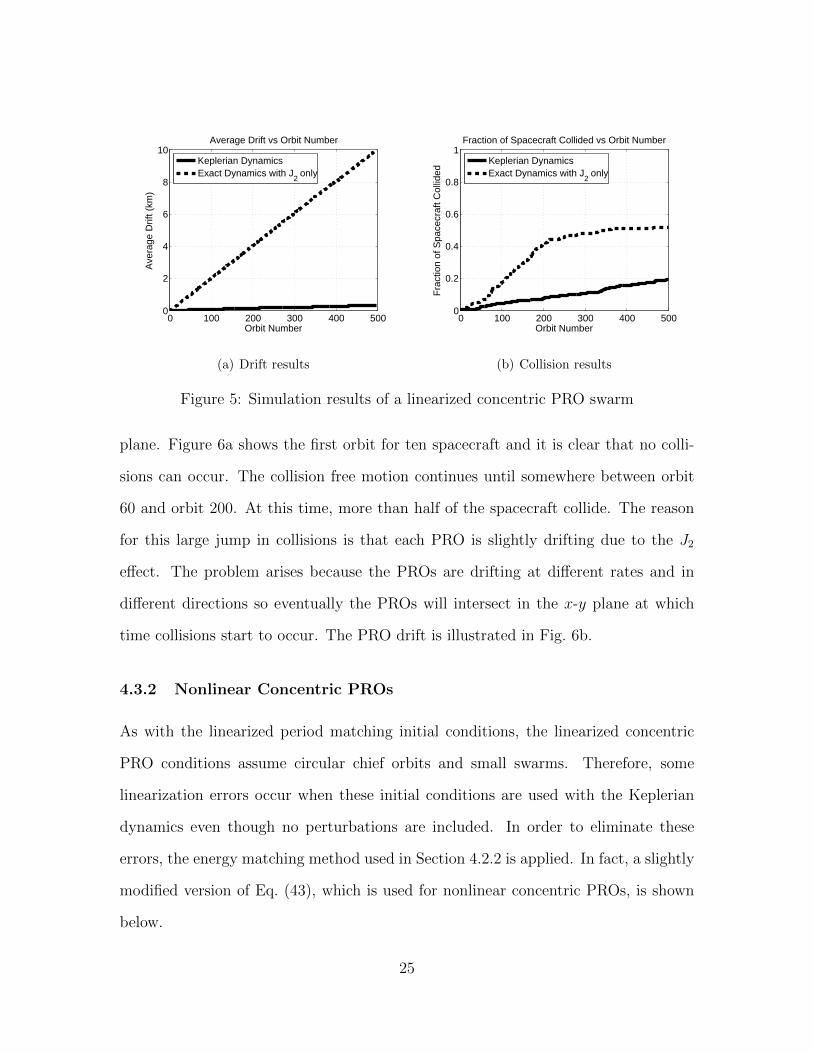
Figure 5a shows the drift results for the concentric PRO swarm. These results are

nearly identical to the drift results from a period matched swarm. The drift rate of

the swarm under the influence of J2 is 20.0 m/orbit, which is small compared to the

initial size of the swarm. The average fuel cost per spacecraft of this method is 1.1

m/s which is about a 25% increase compared to the period matched swarm.

On the other hand, the collision results in Fig. 5b show much improvement com-

pared to the previous simulation. The concentric PRO swarm is nearly collision free

(one or two collisions) for the first 60 orbits even with the exact dynamics with J2

only. This collision free motion occurs because the PROs do not intersect in the x-y

24

0 100 200 300 400 5000

2

4

6

8

10Average Drift vs Orbit Number

Orbit Number

Ave

rage

Drif

t (km

)

Keplerian DynamicsExact Dynamics with J

2 only

(a) Drift results

0 100 200 300 400 5000

0.2

0.4

0.6

0.8

1

Orbit Number

Fra

ctio

n of

Spa

cecr

aft C

ollid

ed

Fraction of Spacecraft Collided vs Orbit Number

Keplerian DynamicsExact Dynamics with J

2 only

(b) Collision results

Figure 5: Simulation results of a linearized concentric PRO swarm

plane. Figure 6a shows the first orbit for ten spacecraft and it is clear that no colli-

sions can occur. The collision free motion continues until somewhere between orbit

60 and orbit 200. At this time, more than half of the spacecraft collide. The reason

for this large jump in collisions is that each PRO is slightly drifting due to the J2

effect. The problem arises because the PROs are drifting at different rates and in

different directions so eventually the PROs will intersect in the x-y plane at which

time collisions start to occur. The PRO drift is illustrated in Fig. 6b.

4.3.2 Nonlinear Concentric PROs

As with the linearized period matching initial conditions, the linearized concentric

PRO conditions assume circular chief orbits and small swarms. Therefore, some

linearization errors occur when these initial conditions are used with the Keplerian

dynamics even though no perturbations are included. In order to eliminate these

errors, the energy matching method used in Section 4.2.2 is applied. In fact, a slightly

modified version of Eq. (43), which is used for nonlinear concentric PROs, is shown

below.

25

−2 −1 0 1 2−2

−1

0

1

2R

adia

l (km

)

Alongtrack (km)

Projection of PROs onto x−y Plane

(a) First Orbit

−2 −1 0 1 2

−2

−1

0

1

2

Alongtrack (km)

Rad

ial (

km)

Projection of PROs onto x−y Plane

Orbit 1Orbit 60

(b) Orbit Drift

Figure 6: The projection in the x-y plane of concentric PROs

x0,N,CP =‖~Vr‖‖~VL,CP ‖

x0,L,CP +

(‖~Vr‖‖~VL,CP ‖

− 1

)(vx − y0ωz)

y0,N,CP =‖~Vr‖‖~VL,CP ‖

y0,L,CP +

(‖~Vr‖‖~VL,CP ‖

− 1

)(h

r+ x0ωz − z0ωx

)(46)

z0,N,CP =‖~Vr‖‖~VL,CP ‖

z0,L,CP +

(‖~Vr‖‖~VL,CP ‖

− 1

)y0ωx

where

~VL,CP = (vx + x0,L,CP − y0ωz)x+ (h

r+ y0,L,CP + x0ωz − z0ωx)y + (z0,L,CP + y0ωx)z (47)

and ‖~Vr‖ is defined in Eq. (40).

Then, using the conditions in Eq. (45), Eq. (46) results in the following equation.

26

x0,N,CP =‖~Vr‖‖~VL,CP ‖

(1

2ωzy0

)+

(‖~Vr‖‖~VL,CP ‖

− 1

)(vx − y0ωz)

y0,N,CP =‖~Vr‖‖~VL,CP ‖

(−2ωzx0) +

(‖~Vr‖‖~VL,CP ‖

− 1

)(h

r+ x0ωz − z0ωx

)(48)

z0,N,CP =

(‖~Vr‖‖~VL,CP ‖

− 1

)y0ωx

Applying the initial conditions in Eq. (48) to the nominal swarm gives the results

that are very similar to those seen in Fig. 5. As with period matching, the nonlinear

conditions eliminate errors caused by linearization but does not dramatically improve

the collision or drift behavior of the swarm under exact dynamics with J2 only.

Although the concentric PROs method provides functional swarm motion for 60

orbits, it is not sufficient for a full mission. The amount of collisions occurring between

orbit 60 and orbit 200 will definitely prevent the swarm from functioning; therefore,

this approach will not work for any mission longer than a few days. In Section 5,

initial conditions will be developed which provide collision free orbits for missions

which last for months. Additionally, the PROs will drift at different rates depending

on the orbital elements of the chief orbit. Therefore, this jump in the collision fraction

can occur as early as the 10 orbit mark. The concentric PROs can provide desired

trajectories for use in a feedback controller [22] but on its own it does not achieve

good swarm keeping performance. Instead, the effects of the J2 dynamics need to be

taken into account when deriving initial conditions for collision free swarm keeping.

27

5 Swarm Keeping Methods for J2 Perturbed

Orbits

In the previous section, initial conditions were derived for collision free swarm motion

using the Keplerian dynamics. The effectiveness of these conditions in a J2 perturbed

environment was tested by numerically integrating the exact dynamics with J2 only.

After making several adjustments to the initial conditions, it was determined that

the J2 effect will cause spacecraft to collide and drift apart after a certain number

of orbits. In this section, the initial conditions derived in Section 4 are modified to

take into account the effects of J2 on the swarm motion. Atmospheric drag will be

discussed in Section 6 but it is neglected in this section because the accelerations

due to J2 are several orders of magnitude larger than those caused by drag. The

J2 perturbation affects relative motion in two ways: the crosstrack motion becomes

coupled with the in-plane motion and the gravity gradient direction and magnitude

are no longer constant.

5.1 Effects of Crosstrack Motion

In the HCW equations or Keplerian dynamics, the crosstrack, or out of plane motion,

is uncoupled from the in plane motion. However, with the addition of the J2 terms

the motion becomes coupled in all three directions. This causes a growth in the

crosstrack oscillation [7], which will cause secular drift in the alongtrack direction if

it is not accounted for. In order to eliminate this growth, the equation for the first

order approximation of the crosstrack motion is written as follows.

z = r sin θδi− r cos θ sin iδΩ (49)

28

In this equation, δi and δΩ represent the differential inclination and right ascension,

respectively. The only term in Eq. (49) that can have a secular drift is δΩ (see the

equations of motion of the chief orbit in Section 3.1) since r and i do not have secular

terms due to J2. Taking the derivative of δΩ results in

δΩ = Ωj − Ω (50)

where Ωj is the right ascension of the deputy spacecraft. Substituting in for Ω and

Ωj using GVEs, integrating over an entire orbit to obtain the secular drift, setting

the secular drift to zero, and simplifying yields

z(t) = B cos θ(t) = B cos (ωzt+ θ0) (51)

where B is a constant and θ0 is the initial argument of latitude of the chief space-

craft. This equation specifies that the crosstrack motion must have a certain phase

with respect to the orbital motion in order to avoid growth in the amplitude of the

crosstrack motion.

The following equation for crosstrack motion comes from Eq (35).

z(t) = z0 cosωzt+z0

ωzsinωzt (52)

Equating Eq. (51) and Eq. (52), and applying the two conditions in Eq. (45) result

in the following conditions.

x0,L,J2 =1

2ωzy0, y0,L,J2 = −2ωzx0, z0,L,J2 = −ωzz0 tan θ0 (53)

The results of applying Eq. (53) are shown in Fig. 7. In Fig. 7a, the drift rate

of the swarm is 15.5 m/orbit. This is a slight improvement over the period matched

29

0 100 200 300 400 5000

1

2

3

4

5

6

7

8Average Drift vs Orbit Number

Orbit Number

Ave

rage

Drif

t (km

)

Keplerian DynamicsExact Dynamics with J

2 only

(a) Drift results

0 100 200 300 400 5000

0.2

0.4

0.6

0.8

1

Orbit Number

Fra

ctio

n of

Spa

cecr

aft C

ollid

ed

Fraction of Spacecraft Collided vs Orbit Number

Keplerian DynamicsExact Dynamics with J

2 only

(b) Collision results

Figure 7: Simulation results of a linearized concentric PRO swarm with no crosstrackdrift

and concentric PRO swarms. Additionally, Fig. 7b shows that the collision fraction

remains under 0.1 for the first 80 orbits and remains under 0.5 for the entire 500 orbit

simulation. Additionally, the fuel required to perform this method is 1.55 m/s, which

is about a 40% increase compared to a concentric PRO swarm. Once again, the drift

and collision results are improved compared to the previous methods. However, these

results must be improved further if the initial conditions are to provide collision free

motion.

It is important to note that the third condition in Eq. (53) depends on tan θ0

and therefore can potentially require an infinite velocity. For this reason, it is rec-

ommended that the burn be applied at the equator, if possible, in order to minimize

the fuel used. Additionally, if the burn must be applied when | tan θ0| > 1, it is

recommended that | tan θ0| = 1 be used and then an additional burn be applied once

| tan θ| ≤ 1. For, some applications, such as projected circular orbits (PCO), it is

desired that the y − z projection be a circle. In this case the required velocity in

the crosstrack direction is fixed by the desired shape of the swarm. Therefore, the

30

burn time, or θ0, is chosen so that Eq. (53) is not violated and a circular projection

is achieved. In this example it is likely that the burn will be non equatorial.

5.2 Effects of Gravity Gradient on Swarm Motion

Another difference that arises with the addition of J2 is the change in the gravity

gradient vector caused by the J2 disturbance. For a spherical Earth the gravity

gradient vector has a constant direction and the magnitude depends only on r. The

Keplerian gravity gradient vector is shown below.

∇U =µ

r2x (54)

The gradient of the gravitational potential under the influence of J2 is shown

in Eq. (14). Since ∇UJ2 is not aligned with the radial direction, a new coordinate

system (x′′, y′′, z′′) is defined so that x′′ is aligned with ∇UJ2 and y′′ remains in

the orbital plane. This new coordinate system is achieved by rotating the LVLH

frame counterclockwise about the z axis by the angle α resulting in the intermediate

coordinate system (x′, y′, z′). Then, this coordinate system is rotated clockwise about

the y′ axis by an angle β to arrive at the desired coordinate system (x′′, y′′, z′′). The

angles α and β are functions of the chief’s orbital parameters and are defined as

follows:

α = arctan

(∇UJ2 · y∇UJ2 · x

)(55)

β = arctan

(∇UJ2 · z√

(∇UJ2 · x)2 + (∇UJ2 · y)2

)(56)

Now that there exists a coordinate system aligned with the gravitational potential

31

gradient, Eq. (53) is applied using the new coordinate system to get

x′′0,L,J2

y′′0,L,J2

z′′0,L,J2

=

0 1

2ω′′z 0

−2ω′′z 0 0

0 0 −ω′′z tan θ0

x′′0

y′′0

z′′0

(57)

where the orbital angular rate ω′′z is

ω′′z =

√‖∇UJ2‖

r(58)

Next, Eq. (57) is transformed back into the LVLH coordinates. To do this, the

transformation equations for both rotations are needed. The first and second rotation

are described by Eq. (59) and Eq. (60), respectively.

x′

y′

z′

=

cosα sinα 0

− sinα cosα 0

0 0 1

x

y

z

(59)

x′′

y′′

z′′

=

cosβ 0 sinβ

0 1 0

− sinβ 0 cosβ

x′

y′

z′

(60)

Substituting Eq. (60) into the right hand side of Eq. (57) yields

x′′0,L,J2

y′′0,L,J2

z′′0,L,J2

=

0 1

2ω′′z 0

−2ω′′z cosβ 0 −2ω′′z sinβ

ω′′z sinβ tan θ0 0 −ω′′z cosβ tan θ0

x′0

y′0

z′0

(61)

and substituting Eq. (59) into the right hand side of Eq. (61) gives

32

x′′0,L,J2

y′′0,L,J2

z′′0,L,J2

=

−1

2ω′′z sinα 1

2ω′′z cosα 0

−2ω′′z cosα cosβ −2ω′′z sinα cosβ −2ω′′z sinβ

ω′′z cosα sinβ tan θ0 ω′′z sinα sinβ tan θ0 −ω′′z cosβ tan θ0

x0

y0

z0

(62)

Now solve for (x0,L, y0,L, z0,L) in terms of (x′′0,L, y′′0,L, z

′′0,L) by inverting Eq. (59) and

substituting in the inverse of Eq. (60).

x0,L,J2

y0,L,J2

z0,L,J2

=

cosα cosβ − sinα − cosα sinβ

sinα cosβ cosα − sinα sinβ

sinβ 0 cosβ

x′′0,L,J2

y′′0,L,J2

z′′0,L,J2

(63)

Finally, substituting Eq. (62) into the right hand side of Eq. (63) results in the

desired initial conditions shown below.

x0,L,J2

y0,L,J2

z0,L,J2

= ω′′z

32cαsαcβ − c

2αs

2βtθ0

12c

2αcβ + 2s2

αcβ − cαsαs2βtθ0 2sαsβ + cαcβsβtθ0

−2c2αcβ − 1

2s2αcβ − cαsαs2

βtθ0 −32cαsαcβ − s

2αs

2βtθ0 −2cαsβ + sαcβsβtθ0

−12sαsβ + cαcβsβtθ0

12cαsβ + sαcβsβtθ0 −c2

βtθ0

x0

y0

z0

(64)

where s(·),c(·), and t(·) represent sin(·), cos(·), and tan(·), respectively. These initial

conditions are applied to the nominal swarm and the results are shown in Fig. 8.

Figure 8a shows the drift results for a nomianl swarm. After 500 orbits, the swarm

drifts by 2.6 m/orbit under the influence of J2. This is a significant improvement over

previous methods. However, the collision results of the J2 adjusted swarm, shown in

Fig. 8b, show that the collision fraction remains under 0.1 for 100 orbits but eventually

reaches 0.75, which is not acceptable for a functioning swarm. The fuel usage is 1.55

m/s which is similar to the method in Section 5.1. These results show that the J2

33

0 100 200 300 400 5000

2

4

6

8

10Average Drift vs Orbit Number

Orbit Number

Ave

rage

Drif

t (km

)

Keplerian DynamicsExact Dynamics with J

2 only

(a) Drift results

0 100 200 300 400 5000

0.2

0.4

0.6

0.8

1

Orbit Number

Fra

ctio

n of

Spa

cecr

aft C

ollid

ed

Fraction of Spacecraft Collided vs Orbit Number

Keplerian DynamicsExact Dynamics with J

2 only

(b) Collision results

Figure 8: Simulation results of a swarm accounting for linearized J2 effects

adjusted method is still not sufficient for collision free motion.

5.3 Energy Matching with J2

The initial conditions from Eq. (64) greatly decrease the drift rate of the swarm by

accounting for the change in magnitude and direction of the gravity gradient vector

caused by the J2 effect. The major problem with these equations is that they use

Eq. (53) as a starting point. Therefore, these J2 adjusted conditions assume a circular

chief orbit and they are linearized. In order to eliminate these potential sources of

error, a new set of initial conditions are derived using nonlinear energy matching

instead of using the HCW equations to eliminate drift.

In order to ensure that the spacecraft do not drift apart, the total energy of each

deputy spacecraft is matched to the energy of the chief spacecraft. In the following

energy matching condition, ‖~Vr‖ is defined in Eq. (40) and ~V is defined in Eq. (37).

‖~V ‖2

2+ U =

‖~Vr,J2‖2

2+ Uj (65)

34

where U is defined below and Uj is defined in Eq. (28).

U = −µr− kJ2

r3

(1

3− sin2 i sin2 θ

)(66)

Equation (65) can be rewritten as

‖~Vr,J2‖ =

√‖~V ‖2 + 2(U − Uj) (67)

Now that the desired velocity for an energy matched spacecraft in the presence of J2

has been established, the modified version of Eq. (43) is applied as shown below

x0,N,J2 =‖~Vr,J2‖‖~VL,J2‖

x0,L,J2 +

(‖~Vr,J2‖‖~VL,J2‖

− 1

)(vx − y0ωz)

y0,N,J2 =‖~Vr,J2‖‖~VL,J2‖

y0,L,J2 +

(‖~Vr,J2‖‖~VL,J2‖

− 1

)(h

r+ x0ωz − z0ωx

)(68)

z0,N,J2 =‖~Vr,J2‖‖~VL,J2‖

z0,L,J2 +

(‖~Vr,J2‖‖~VL,J2‖

− 1

)y0ωx

where

~VL,J2 = (vx + x0,L,J2 − y0ωz)x+ (h

r+ y0,L,J2 + x0ωz − z0ωx)y + (z0,L,J2 + y0ωx)z (69)

Then, applying the conditions in Eq. (64) to Eq. (68) results in the main J2 invariant

swarm keeping equations. The following J2 invariant equations use energy matching

to build upon the results from Eq. (53) and Eq. (64).

35

0 100 200 300 400 5000

1

2

3

4

5

6

7

8Average Drift vs Orbit Number

Orbit Number

Ave

rage

Drif

t (km

)

Keplerian DynamicsExact Dynamics with J

2 only

(a) Drift results

0 100 200 300 400 5000

0.2

0.4

0.6

0.8

1

Orbit Number

Fra

ctio

n of

Spa

cecr

aft C

ollid

ed

Fraction of Spacecraft Collided vs Orbit Number

Keplerian DynamicsExact Dynamics with J

2 only

(b) Collision results

Figure 9: Simulation results of an energy matched swarm

x0,N,J2 =‖~Vr,J2‖‖~VL,J2‖

[(3

2cαsαcβ − c2

αs2βtθ0

)x0 +

(1

2c2αcβ + 2s2

αcβ − cαsαs2βtθ0

)y0

+ (2sαsβ + cαcβsβtθ0) z0

]ω′′z +

(‖~Vr,J2‖‖~VL,J2‖

− 1

)(vx − y0ωz)

y0,N,J2 =‖~Vr,J2‖‖~VL,J2‖

[(−2c2

αcβ −1

2s2αcβ − cαsαs2

βtθ0

)x0 +

(−3

2cαsαcβ − s2

αs2βtθ0

)y0 (70)

+ (−2cαsβ + sαcβsβtθ0) z0

]ω′′z +

(‖~Vr,J2‖‖~VL,J2‖

− 1

)(h

r+ x0ωz − z0ωx

)

z0,N,J2 =‖~Vr,J2‖‖~VL,J2‖

[(−1

2sαsβ + cαcβsβtθ0

)x0 +

(1

2cαsβ + sαcβsβtθ0

)y0

+(−c2

βtθ0)z0

]ω′′z +

(‖~Vr,J2‖‖~VL,J2‖

− 1

)y0ωx

where α and β are defined in Eq. (55) and Eq. (56), respectively. Additionally, s(·),c(·),

and t(·) represent sin(·), cos(·), and tan(·), respectively.

The energy matching conditions in Eq. (70) show a significant improvement in

collision and drift results compared to the linearized conditions. This is because the

drift due to J2 has been significantly reduced so that the errors due to linearization and

36

eccentricity are dominant. Therefore, eliminating these errors by using the nonlinear

conditions has a huge impact on the performance of the swarm and the drift rate in

Fig. 9a is 7.55 mm/orbit, which is about three orders of magnitude better than any

other methods. Additionally, Fig. 9b shows that the collision fraction remains under

2% for 500 orbits. Additionally, the fuel usage is about 1.55 m/s, which is comparable

to the previous methods. Therefore, the energy matched conditions prevent collisions

for more than 500 orbits while still using only a single burn of similar magnitude to

the other methods.

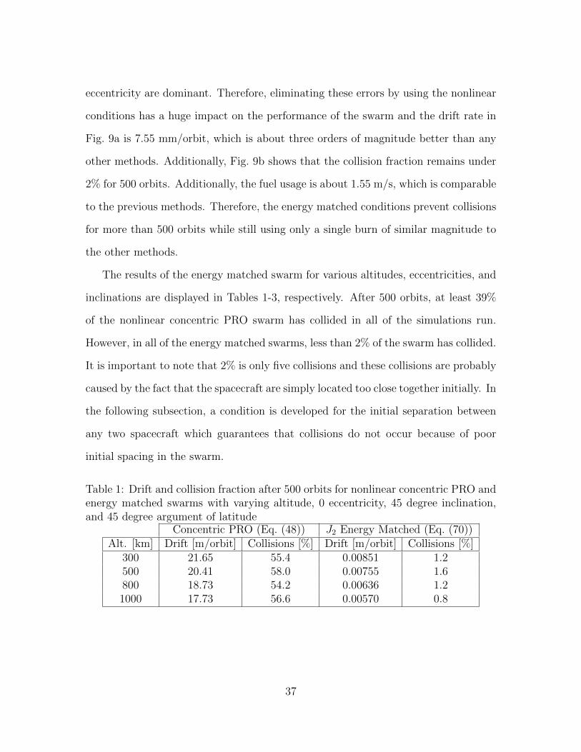
The results of the energy matched swarm for various altitudes, eccentricities, and

inclinations are displayed in Tables 1-3, respectively. After 500 orbits, at least 39%

of the nonlinear concentric PRO swarm has collided in all of the simulations run.

However, in all of the energy matched swarms, less than 2% of the swarm has collided.

It is important to note that 2% is only five collisions and these collisions are probably

caused by the fact that the spacecraft are simply located too close together initially. In

the following subsection, a condition is developed for the initial separation between

any two spacecraft which guarantees that collisions do not occur because of poor

initial spacing in the swarm.

Table 1: Drift and collision fraction after 500 orbits for nonlinear concentric PRO andenergy matched swarms with varying altitude, 0 eccentricity, 45 degree inclination,and 45 degree argument of latitude

Concentric PRO (Eq. (48)) J2 Energy Matched (Eq. (70))Alt. [km] Drift [m/orbit] Collisions [%] Drift [m/orbit] Collisions [%]

300 21.65 55.4 0.00851 1.2500 20.41 58.0 0.00755 1.6800 18.73 54.2 0.00636 1.21000 17.73 56.6 0.00570 0.8

37

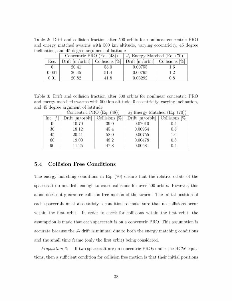
Table 2: Drift and collision fraction after 500 orbits for nonlinear concentric PROand energy matched swarms with 500 km altitude, varying eccentricity, 45 degreeinclination, and 45 degree argument of latitude

Concentric PRO (Eq. (48)) J2 Energy Matched (Eq. (70))Ecc. Drift [m/orbit] Collisions [%] Drift [m/orbit] Collisions [%]

0 20.41 58.0 0.00755 1.60.001 20.45 51.4 0.00765 1.20.01 20.82 41.8 0.03292 0.8

Table 3: Drift and collision fraction after 500 orbits for nonlinear concentric PROand energy matched swarms with 500 km altitude, 0 eccentricity, varying inclination,and 45 degree argument of latitude

Concentric PRO (Eq. (48)) J2 Energy Matched (Eq. (70))Inc. [] Drift [m/orbit] Collisions [%] Drift [m/orbit] Collisions [%]

0 10.70 39.0 0.02010 0.430 18.12 45.4 0.00954 0.845 20.41 58.0 0.00755 1.660 19.00 48.2 0.00478 0.890 11.25 47.8 0.00581 0.4

5.4 Collision Free Conditions

The energy matching conditions in Eq. (70) ensure that the relative orbits of the

spacecraft do not drift enough to cause collisions for over 500 orbits. However, this

alone does not guarantee collision free motion of the swarm. The initial position of

each spacecraft must also satisfy a condition to make sure that no collisions occur

within the first orbit. In order to check for collisions within the first orbit, the

assumption is made that each spacecraft is on a concentric PRO. This assumption is

accurate because the J2 drift is minimal due to both the energy matching conditions

and the small time frame (only the first orbit) being considered.

Proposition 3: If two spacecraft are on concentric PROs under the HCW equa-

tions, then a sufficient condition for collision free motion is that their initial positions

38

satisfy [20] √δx2

0 + δy20 > 2X (71)

where√δx2

0 + δy20 is the initial projected distance between two spacecraft and X is

the minimum distance at which two spacecraft will collide. This condition ensures

that two spacecraft will never come within a distance X of each other for all time.

Proposition 3 is proved rigorously in Acikmese et al.[20] under the HCW equations.

However, it is useful to invoke here as a heuristic to ensure that there are no poor

initial conditions when initializing a swarm with respect to Keplerian or exact relative

dynamics. Combining the condition in Eq. (71) with the J2 energy matched conditions

in Eq. (70) provides collision free motion. Depending on the length of the mission,

the relative semi-major axis and phase of each spacecraft can be chosen so that they

will not collide for the duration of the mission. This can be done by calculating the

worst case drift and placing the spacecraft on PROs whose semi-major axes differ by

more than the worst case drift. This will ensure that the PROs never drift far enough

to intersect with another PRO and therefore no collisions will occur.

39

6 Swarm Keeping for J2 and Atmospheric Drag

Perturbed Orbits

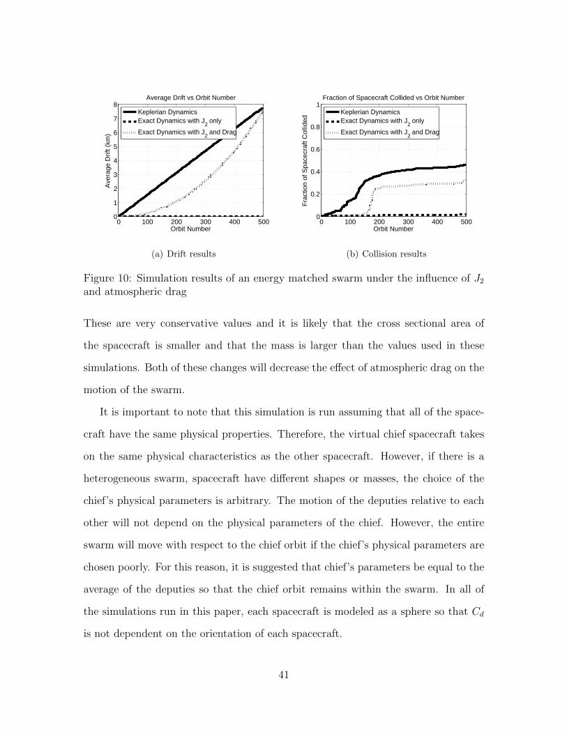
This section shows the effects of atmospheric drag on energy matched swarms. Al-

though atmospheric drag effects are several orders of magnitude smaller than J2 ef-

fects, atmospheric drag is a non-conservative force, which means that energy matching

the spacecraft cannot be used to account for atmospheric drag effects. In order to

account for atmospheric drag, a multi-burn guidance method is developed in order to

maintain collision free motion.

6.1 Effects of Atmospheric Drag

The conditions developed in Eq. (70) have been shown to eliminate collisions for

spacecraft swarms in the presence of J2. In this section, the effects of atmospheric

drag on an energy matched swarm are investigated. In order to do this, the energy

matching conditions are applied to the swarm but this time atmospheric drag is

included in the simulation. The collision and drift results from this simulation are

shown in Fig. 10.

Figure 10 shows that the addition of atmospheric drag causes the swarm to dis-

perse which then causes the spacecraft to collide after only 100 orbits. Therefore,

the energy matching conditions do not prevent collisions when atmospheric drag is

significant. Since atmospheric drag is dependent on many factors including space-

craft mass, cross-sectional area, and altitude, there may be certain missions where

the effect of atmospheric drag is so small that the energy matching conditions provide

collision free motion. For this simulation, the values of the cross sectional area (A)

and mass (m) of the spacecraft were chosen to be 0.01 [m2] and 0.1 [kg], respectively.

40

0 100 200 300 400 5000

1

2

3

4

5

6

7

8Average Drift vs Orbit Number

Orbit Number

Ave

rage

Drif

t (km

)

Keplerian DynamicsExact Dynamics with J

2 only

Exact Dynamics with J2 and Drag

(a) Drift results

0 100 200 300 400 5000

0.2

0.4

0.6

0.8

1

Orbit Number

Fra

ctio

n of

Spa

cecr

aft C

ollid

ed

Fraction of Spacecraft Collided vs Orbit Number

Keplerian DynamicsExact Dynamics with J

2 only

Exact Dynamics with J2 and Drag

(b) Collision results

Figure 10: Simulation results of an energy matched swarm under the influence of J2

and atmospheric drag

These are very conservative values and it is likely that the cross sectional area of

the spacecraft is smaller and that the mass is larger than the values used in these

simulations. Both of these changes will decrease the effect of atmospheric drag on the

motion of the swarm.

It is important to note that this simulation is run assuming that all of the space-

craft have the same physical properties. Therefore, the virtual chief spacecraft takes

on the same physical characteristics as the other spacecraft. However, if there is a

heterogeneous swarm, spacecraft have different shapes or masses, the choice of the

chief’s physical parameters is arbitrary. The motion of the deputies relative to each

other will not depend on the physical parameters of the chief. However, the entire

swarm will move with respect to the chief orbit if the chief’s physical parameters are

chosen poorly. For this reason, it is suggested that chief’s parameters be equal to the

average of the deputies so that the chief orbit remains within the swarm. In all of

the simulations run in this paper, each spacecraft is modeled as a sphere so that Cd

is not dependent on the orientation of each spacecraft.

41

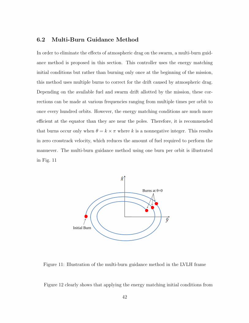
6.2 Multi-Burn Guidance Method

In order to eliminate the effects of atmospheric drag on the swarm, a multi-burn guid-

ance method is proposed in this section. This controller uses the energy matching

initial conditions but rather than burning only once at the beginning of the mission,

this method uses multiple burns to correct for the drift caused by atmospheric drag.

Depending on the available fuel and swarm drift allotted by the mission, these cor-

rections can be made at various frequencies ranging from multiple times per orbit to

once every hundred orbits. However, the energy matching conditions are much more

efficient at the equator than they are near the poles. Therefore, it is recommended

that burns occur only when θ = k × π where k is a nonnegative integer. This results

in zero crosstrack velocity, which reduces the amount of fuel required to perform the

manuever. The multi-burn guidance method using one burn per orbit is illustrated

in Fig. 11

Initial Burn

Burns at θ=0

Figure 11: Illustration of the multi-burn guidance method in the LVLH frame

Figure 12 clearly shows that applying the energy matching initial conditions from

42

0 100 200 300 400 5000

1

2

3

4

5

6

7

8Average Drift vs Orbit Number

Orbit Number

Ave

rage

Drif

t (km

)

Single Burn MethodMultiple Burn Method

(a) Drift results

0 100 200 300 400 5000

0.2

0.4

0.6

0.8

1

Orbit Number

Fra

ctio

n of

Spa

cecr

aft C

ollid

ed

Fraction of Spacecraft Collided vs Orbit Number

Single Burn MethodMultiple Burn Method

(b) Collision results

Figure 12: Simulation results of the multiburn guidance method under the influenceof J2 and atmospheric drag

Eq. (70) once per orbit reduces the drift caused by atmospheric drag and provides

collision free motion for over 500 orbits. This multi-burn guidance method maintains

the size of the swarm and prevents collisions within the swarm in the presence of the

two major perturbations in LEO, J2 effects and atmospheric drag. In the simulation

shown in Fig. 12, the first burn occur at θ = 45 degrees because that is the initial

position but all subsequent burns occur at θ = 0 degrees in order to minimize fuel.

The multi-burn guidance method can be applied regardless of the initial argu-

ment of latitude. If there is no desired swarm shape, the first burn should occur

immediately, regardless of the initial argument of latitude, and the following burns

should occur at the equator in order to minimize fuel. However, it may be desirable

to maintain a specific swarm shape, such as a projected circular orbit. In this case it

may not be possible to achieve this shape and burn at the equator. Therefore, based

on the desired crosstrack velocity, the argument of latitude at which the burn must

occur can be calculated based on Eq. (53). In this scenario, the first burn should

occur immediately and the following burns should occur at the argument of latitude

43

which produces the desired crosstrack motion. This method minimizes fuel usage and

drift while still permitting a variety of swarm shapes.

44

7 Conclusion

In this paper, the swarm keeping problem was explored for a swarm of hundreds of

spacecraft. The notion of swarm keeping was introduced as maintaining relative dis-

tances between multiple spacecraft in the presence of disturbances and ensuring that

collisions do not occur. The number of spacecraft along with their modest capabili-

ties provided new challenges which have not been addressed in previous studies. The

large number of spacecraft makes online path planning or reactive collision avoidance

extremely difficult. Therefore, a set of initial conditions was developed that provide

collision free motion for hundreds of orbits in the presence of J2 perturbations. Fur-

thermore, such initial conditions coincide with a fuel-efficient strategy since very little

fuel is required to stay on J2 invariant relative orbits.

The main results developed in Section 5 establish J2 invariant relative orbits by

applying the energy matching method after correcting for the effects of the gravity

gradients and J2-perturbed cross-track motions. The proposed swarm keeping initial

conditions were shown by computer simulation to greatly reduce both the swarm drift

rate and the collision rate across a wide range of reference orbits regardless of altitude,

eccentricity, and inclination (e.g., a drift rate of 7.55 mm/orbit and a collision fraction

of 1.6% for the reference orbit of 500 km, 0 eccentricity, and 45 deg inclination).

The performance of collision free motions can deteriorate over time in the presence

of air drag especially in lower LEO. Another contribution of the paper lies in deriv-

ing a new set of nonlinear dynamics which include both J2 effects and atmospheric

drag. This new dynamic model was used to test the energy matching conditions

in the presence of atmospheric drag. Finally, a multi-burn guidance method, which

sequentially employs the main initial conditions of J2 invariant relative orbits, was

developed to correct for the effects of atmospheric drag. This controller was shown

45

by computer simulation to provide collision free motion over hundreds of orbits for

spacecraft swarms in the presence of the two dominant disturbances in LEO, J2 and

atmospheric drag.

46

References

[1] Aung, M., Ahmed, A., Wette, M., Scharf, D., Tien, J., Purcell, G., Regehr, M.,

and Landin, B., “An Overview of Formation Flying Technology Development

for the Terrestrial Planet Finder Mission,” Proceedings of the IEEE Aerospace

Conference, 2004, pp. 2667–2679.

[2] Hughes, S. P., “Preliminary Optimal Orbit Design for the Laser Interferometer

Space Antenna (LISA),” AAS Rocky Mountain Guidance and Control Confer-

ence, 2002, pp. 61–78.

[3] Scharf, D. P., Hadaegh, F. Y., and Ploen, S. R., “A Survey of Spacecraft For-

mation Flying Guidance and Control (Part I): Guidance,” Proceedings of the

American Control Conference, Jun. 2003, pp. 1733–1739.

[4] Scharf, D. P., Hadaegh, F. Y., and Ploen, S. R., “A Survey of Spacecraft For-

mation Flying Guidance and Control (Part II): Control,” Proceedings of the

American Control Conference, Jun. 2004, pp. 2976–2984.

[5] Chung, S.-J., Ahsun, U., and Slotine, J.-J. E., “Application of Synchronization

to Formation Flying spacecraft: Lagrangian Approach,” Journal of Guidance,

Control, and Dynamics , Vol. 32, No. 2, Mar.-Apr. 2009, pp. 512–526.

[6] Schaub, H., Vadali, S. R., Junkins, J. L., and Alfriend, K. T., “Spacecraft Forma-

tion Flying Control using Mean Orbital Elements,” Journal of the Astronautical

Sciences , Vol. 48, No. 1, Jan.-Mar. 2000, pp. 69–87.

[7] Vadali, S. R., Alfriend, K. T., and Vaddi, S., “Hill’s Equations, Mean Orbital

Elements, and Formation Flying of Satellites,” Advances in the Astronautical

Sciences , Vol. 106, 2000, pp. 187–203.

47

[8] Afriend, K. T., Vadali, S. R., and Schaub, H., “Formation Flying Satellites:

Control by an Astrodynamicist,” Celestial Mechanics and Dynamical Astron-

omy , Vol. 81, 2001, pp. 57–62.

[9] Schaub, H. and Alfriend, K. T., “J2 Invariant Relative Orbits for Spacecraft For-

mations,” Celestial Mechanics and Dynamical Astronomy , Vol. 79, 2001, pp. 77–

95.

[10] Breger, L., How, J. P., and Alfriend, K. T., “Partial J2-Invariance for Space-

craft Formations,” Proceedings of the AIAA Guidance, Navigation and Control

Conference and Exhibit , Aug. 2006.

[11] Breger, L. and How, J. P., “Gauss’s Variational Equation-Based Dynamics and

Control for Formation Flying Spacecraft,” Journal of Guidance, Control, and

Dynamics , Vol. 30, No. 2, Mar.-Apr. 2007, pp. 437–448.

[12] Hadaegh, F. Y., Chung, S.-J., and Manaroha, H., “Development and Flight of

Swarms of 100-gram Class Satellites,” IEEE Systems Journal (to be submitted),

2011.

[13] Clohessy, W. and Wiltshire, R., “Terminal Guidance System for Satellite Ren-

dezvous,” Journal of Astronautical Sciences , Vol. 27, No. 9, 1960, pp. 653–658.

[14] Tschauner, J. and Hempel, P., “Rendezvous Zu Einem In Elliptischer Bahn

Umlaufenden Ziel,” Acta Astronautica, Vol. 11, No. 2, 1965, pp. 104–109.

[15] Schweighart, S. and Sedwick, R., “High-Fidelity Linearized J2 Model for Satellite

Formation Flight,” Journal of Guidance, Control, and Dynamics , Vol. 25, No. 6,

Nov.-Dec. 2002, pp. 1073–1080.

48

[16] Hamel, J.-F. and Lafontaine, J. D., “Linearized Dynamics of Formation Flying

Spacecraft on a J2-Perturbed Elliptical Orbit,” Journal of Guidance, Control,

and Dynamics , Vol. 30, No. 6, Nov.-Dec. 2007, pp. 1649–1658.

[17] Gim, D. and Alfriend, K., “State Transition Matrix of Relative Motion for the

Perturbed Noncircular Reference Orbit,” Journal of Guidance, Control, and Dy-

namics , Vol. 26, No. 6, Nov.-Dec. 2003, pp. 956–971.

[18] Xu, G. and Wang, D., “Nonlinear Dynamic Equations of Satellite Relative Mo-

tion Around an Oblate Earth,” Journal of Guidance, Control, and Dynamics ,

Vol. 31, No. 5, Sep.-Oct. 2008, pp. 1521–1524.

[19] Chang, I., Chung, S.-J., and Blackmore, L., “Cooperative Control with Adaptive

Graph Laplacians for Spacecraft Formation Flying,” 49th IEEE Conference on

Decision and Control , Atlanta, GA, December 2010, pp. 4926–4933.

[20] Acikmese, B., Bayard, D. S., and Hadaegh, F. Y., “On the Evolution of Orbiting

Spacecraft Swarms,” Jet Propulsion Lab, Internal Document (in preparation),

2011.

[21] Kechichian, J. A., “Motion in General Elliptic Orbit with respect to a Drag-

ging and Precessing Coordinate Frame,” Journal of the Astronautical Sciences ,

Vol. 46, No. 1, Jan.-Mar. 1998, pp. 25–45.

[22] Chang, I., Chung, S.-J., and Hadaegh, F., “Phase Synchronization Control of

Robotic Networks on Periodic Ellipses with Adaptive Switching Topologies,”

AIAA Guidance, Navigation, and Control Conference (accepted), Portland, OR,

August 2011.

49