Embed Size (px)
Citation preview

NASA Conrractor Report 3209
Svstem Theory as Applied v
lkkrential Geometry
Robert Hermann
GR,%NT NSG-2252 NOVJMBER 1979
Nkwn. CR 3209 c.1
https://ntrs.nasa.gov/search.jsp?R=19800004522 2018-06-22T00:51:24+00:00Z

TECH LIBRARY KAFB, NM
NASA Contractor Report 3209
System Theory as Applied Differential Geometry
Robert Hermann Americm Mathematical Society Providence, Rhode Isfund
Prepared for Ames Research Center under Grant NSG-22 5 2
NASA ’ National Aeronautics and Space Administration
Scientific and Technical Information Branch
1979

TABIE OF CONTENTS
Page
SUMMARY
1. INTRODUCTION
2. SOME GENERAL PRINCIPLES OF SYSTEM THEORY
3. NOTIONS OF LINEAR SYSTEM THEORY
4. STATE FEEDBACK AND LUENBERGER OBSERVERS OF LINEAR SYSTEMS
5. THE KRONECKER THEORY OF PENCILS OF LINEAR MAPS
6. THE VECTOR BUNDLE ASSOCIATED WITH PAIRS OF LINEAR MAPS
7. THE HOLOMORPHIC VECTOR BUNDLE INVARIANTS OF LINEAR, TIME-INVARIANT INPUT SYSTEMS
8. FEEDBACK EQUIVALENCE AND THE KRONECKER THEORY OF PAIRS OF LINEAR MAPS
9. TRANSFER FUNCTIONS AND HOLOMORPHIC VECTOR BUNDLES FOR 1-D AND n-D SYSTEMS
10. VECTOR BUNDLES ON ORBIT SPACES
11. VECTOR BUNDLES DEFINED BY SYSTEMS OF PARTIAL DIFFERENTIAL EQUATIONS AND LINEAR GROUPS OF SYMMETRIES
12. SO(3,tt:) -BUNDLES
13. THE COMPACTIFIED VECTOR BUNDLE DETERMINED BY THE HELMHOLTZ EQUATION
14. LINEAR FILTERS AND GROUPS
15. CONCLUDING REMARKS
Appendix. GENERALIZATION OF THE PSEUDO-INVERSE CONSTRUCTION TO RIEMANNIAN MANIFOLDS; SLICES AND CANONICAL FORMS FOR GROUP ACTIONS
1
1
3
7
12
16
22
26
28
31
39
40
41
44
48
55
57
REFERENCES 61

SYSTEM THEORY AS APPLIED
DIFFERENTIAL GEOMETRY
By Robert Hermann Division of Applied Sciences
Harvard University
SUMMARY
The opening sections sketch the mathematical framework for System Theory. It has long been recognized that there are (at least) three levels at which it is necessary to study systems: Individual systems, systems depending on para- meters, and "adaptive" or "self-tuning" systems. Systematic and thorough mathematical study at the second level is no doubt necessary for successful future attack on the third level; it is in this study that differential- geometric methodology becomes most useful, indeed, probably essential. It is also pointed out that some of the most basic and important problems in System Theory (even at the practical level) involve properties of orbits and orbit spaces of certain types of Lie groups acting on manifolds.
The core of the report is the description of a new technique for computing these orbits for the case of combined feedback and state equivalence groups acting on linear systems. Although it is equivalent to the well-known Brunovsky canonical form, which is an algebraic method, this technique involves differen- tial geometry, particularly the classification of holomorphic vector bundles on the Riemannian sphere due to A. Grothendieck. It also generalizes to distri- buted parameter systems; certain examples are discussed in a tentative way here. Finally, a generalization to Riemannian geometry of the "pseudo-inverse" construction is presented as a possible useful tool in certain identification problems.
1. INTRODUCTION
Looking at history, we can recognize that many areas of mathematics have developed in symbiosis with science and technology. For example, let us cite the development of differential calculus and differential equations in the 18th and 19th centuries in conjunction with analytical mechanics; the development of the theory of linear partial differential equations in conjunction with continuum mechanics and electromagnetism; in the 20th century, functional analysis and differential geometry have been paired with quantum mechanics
I - .._. -... ..-- -.

and relativity, although the relation between the mathematics and physics has not been as close, direct and stimulating as in earlier times.
A new feature in the science and technology of our day is the use of the hybrid scientific-technological "system", analyzed, designed and run by computers. One has only to think of the space program, and the analogy with such 19th century facts as the development of electricity and the automobile, to gain a historical perspective. Just as the hybrid scientific-technological projects of the 19th century stimulated development of the mathematical topics cited above, in our day there has arisen an amorphous subject called System and Control Theory. By its nature it sprawls over disciplinary boundaries, and is difficult to pin down; one cannot go to the library or to most major universities and systematically learn about it as one would learn, say, differ- ential equations or quantum mechanics. Of course there are textbooks--the treatises by Anderson and Moore [25], Brockett [26], Rosenbrock [272 and Wonham [28] are the best for our purposes. At the research level the journals IEEE Transactions in Automtic Control, SIAM Journal of ControZ and Optimization., and Automatica are standard ones. A striking characteristic of this material is its strong reliance on mathematics, in contrast to other major contemporary areas of science and technology. This is in the nature of the subject--the basic idea is to translate broad areas of science and technology into mathe- matical models that can be handled on the computer in a way that is as indepen- dent as possible of the origin of the models. Most of the research work involves analysis and probability theory, and some relatively concrete aspects of algebra (e.g., matrix theory, combinatorics) that were developed in the 19th century. (In fact, Gantmacher's treatise [ 61 is the only complete reference for some of the algebraic ideas.) However, there has also been a contact with differential geometry which has played a role in guiding research in the discipline. Thisreport will focus on certain aspects of this interface with geometry, with emphasis on work that I have done with Clyde Martin on the geometry of Zinear systems. I will try to concentrate on areas which I believe have the greatest potential utility combined with the possibility of providing new research insights into System Theory. My overall thesis is that modern differential geometry is, among all areas of contemporary mathematics, the best qualified to provide new thought in diverse areas of science and technology.
A short glance at the literature suggests that probability theory and matrix algebra are closely linked to system and control theory, but why differ- ential geometry? Now, differential geometry is most commonly thought of as the study of curves and surfaces in "our" Euclidean three space. Although it has expanded enormously in recent times, allied at times with topology, group-theory, and algebraic geometry, this classical theme remains the core. The point I want to bring to the foreground in this report is that system and control theory also involve curves and surfaces--in more exotic spaces, it is true, but the method- ology of "modern" differential geometry has been oriented precisely to the task of making this generalization.
This methodology has involved the theory of what mathematicians call differential manifolds. Unfortunately this is a difficult subject to learn, since it involves fragments from all the major mathematical disciplines. At the point in this report that we get down to the real work, it will be necessary to assume that the reader has at least some acquaintance with its principles and notation --the treatises by Boothby 1201, Dieudonng [21], and the author [22]
2

may be cited. We shall also make use of material which interfaces differential and algebraic geometry--the standard reference is now the very recent book by GriffithsandHarris [23].
In geometry, a manifold is a space that looks locally like a piece of Euclidean space, but globally may not be one. This means that, given any point, one can coordinatize a neighborhood of that point with n real numbers (n is the dimension of the manifold), but that these number labels vary as the point moves over the space. However, as in tensor analysis, one wants to use these number assignments to perform the usual operations of differential and integral calculus. This requires that the number labels one assigns to different points (called coordinate systems) be related to each other in an infinitely differen- tiabZe ("C"") way. So, a space with a topological structure to assure over-all consistency, and a way of attaching local coordinates to points, not uniquely, but changing in a Cm way, is called a differentiabze manifoZd. In modern mathematics, it has been found to be just about the most appropriately "general" geometric object to study, in the sense that it includes the class of Euclidean space and most of the other spaces (e.g., spheres, tori, surfaces) which appear most frequently, and yet its "differential" and "integral" structure can be studied in a unified way.
The basic idea in differential geometry is to study geometric objects with anu~ytic techniques. (The idea of "curvature" of a curve or surface is a familiar example.) Often, it is most convenient to mediate between the geometry and analysis with algebra. (In fact, it was Descartes, in the 17th century, who taught us to do this.)
2. SOME GENERAL PRINCIPLES OF SYSTEM THEORY
System theory may be thought of as the study of machines, devices, auto- mata, computers, physical objects, etc., behavior.
from the point of view of input-output The famous "black box" is the key concept--a device which accepts
certain inputs, subjects them to certain operations which depend on the "state" at which the box finds itself, and then puts out an output
> r--j ) output input
The theory can be developed in this abstract context as a theory of mappings
9: (space of inputs) x (state) -f (space of outputs)
However, for the purposes of geometry it is most convenient to work in the context of differential equations and continuous time. An input-OutpUt System for us will be a system of ordinary first order differential equations of the form:
3
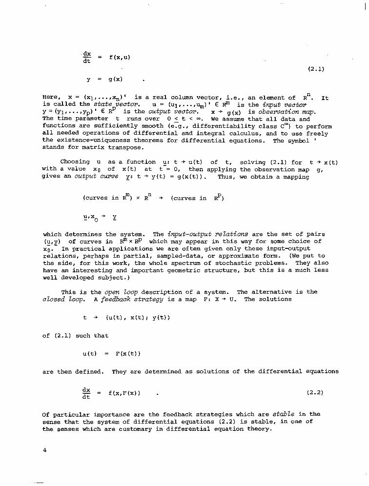
dx dt = f(x,u)
(2.1)
Y = g(x) .
Here, x = (Xl,...,Xn)' n is a real COlmn Vi?CtOr, i.e., an element of R . It is called the state vector. u = (Ul is the input vector Y = (Yl ,...,y,)' E Rp
,..-,I@ E lP is the output vector. is observation map.
The time parameter t runs over x + g(x)
0 < t < m. We assume that all data and functions are sufficiently smooth (e:g., differentiability class C") to perform all needed operations of differential and integral calculus, and to use freely the existence-uniqueness theorems for differential equations. The symbol ' stands for matrix transpose.
Choosing u as a function u: t -f u(t) of t, solving (2.1) for t -t x(t) with a value x0 of x(t) at t-= 0, then applying the observation map g, gives an output curve y: t + y(t) = g(x(t)). Thus, we obtain a mapping
(CUJXeS in Rm) x R" + (curves in #)
urx -+ y -0 -
which determines the system. The input-output relations are the set of pairs (u,y) of curves in ~!"x~p which may appear in this way for some choice of
Xi.- In practical applications we are often given only these input-output relations, perhaps in partial, sampled-data, or approximate form. (We put to the side, for this work, the whole spectrum of stochastic problems. They also have an interesting and important geometric structure, but this is a much less well developed subject.)
This is the open loop description of a system. The alternative is the cZosed loop. A feedback strategy is a map F: X -t U. The solutions
t + (u(t) I x(t) i y(t))
of (2.1) such that
u(t) = F(x(t))
are then defined. They are determined as solutions of the differential equations
dx dt = f(x,F(x)) . (2.2)
Of particular importance are the feedback strategies which are stable in the sense that the system of differential equations (2.2) is stable, in one of the senses which are customary in differential equation theory.
4

-
A basic idea in system theory is to consider a collection, c, of systems and a corresponding collection IO of input-output relations. An important case is that where C depends on a finite number of parameters; call them
h = (Xl,...,Xrl I
For example, C might be defined by differential equations of the following form:
dx dt = f(x,u;)c)
(2.3)
Y = g(.x;h) . 1
Now, two different values X,X' of the parameters might give the same input- output relations. Thus, the corresponding input-output relations might depend on fewer parameters.
The basic object of study in "Geometric" System Theory are parameterized families of systems and input-output relations.
It is in this study of "dependence on parameters" that modern differential geometry--based as it is on differential manifold theory--is so much more powerful than the traditional methodology. Every problem in System Theory has two aspects: First, study solutions for a single system, i.e., for a fixed value of the parameters, then see how this relation varies when the parameters are varied.
For our purposes, it is convenient to focus on three main problems:
A) The Identification ProbZem. Given a set of input-output relations, find a set of systems which realize these relations. Often it is not possible in problems with parameters; singularities are encountered. The goal is then to study how to avoid the singularities or to live with them. For nonlinear systems very little that is of great practical use is known about this problem.
B) The Observer-Compensator Problem. Given a system of form (i-l), design another system
df; dt = P&u,,,
5

where inputs are the inputs and/or outputs of (2.11, fiich perform in‘certain prescribed ways. For example, the "observer-tracker" problems require that $ and x live on the same space, and that
lh (x(t) -y(t)) = 0 t+=
C) The Classic Regulator-Servomeohanism-Optimal Control Problems. I will not go into these in any detail-- see the Treatises by Anderson-Moore 1161 and wonhaln 1191. Here, the traditional theory only is developed in the context of Zinear systems; about everything remains to be done for the nonlinear cases.
Each of these problems also has a "hierarchical" structure suggested by the wide spectrum of applications. I have mentioned the dependence-on-parameters as a "higher" problem than the fixed parameters one. Even "higher" than this are the adaptive and decentrazized-Zarge scale aspects, on which there has been much work (mostofitinconclusive) in the last twenty years. The adaptive problem is probably the most interesting from the philosophical-social point of view (e.g., cybernetics, learning theory), as well as having wide practical ramifications ( automata, _ self-tuning machines, robotics, artificial intelli- gence, etc.). Roughly, this involves a system with unknown, perhaps changing parameters, interaction with some outside system which can sample parts of the input and output. On the basis of these samples, it is desireh--preferably by an iterative process--to estimate the parameters to a first approximation, perhaps then perform certain operations and adjustments, then measure and identify again, etc. hopefully converging on something useful. (There is some analogy with the theory of "measurement" in quantum mechanics; one must consider not only the system in isolation, but in interaction with certain measuring apparatus.)
Having as complete as possible a theory of systems depending on parameters is a necessary condition for a satisfactory adaptive control theory. There has recently been important progress in this area by Feuer and Morse 1241, Goodwin, Ramadge and Caines 1251, involving the analytical and stochastic, discrete-time side of system theory--it may be expected that analogous results may be obtained using geometric ideas for continuous time systems.
Although these concepts obviously have a wide range and validity, carrying them out in an appropriate mathematical context is a slow business which requires formidable mathematical experience and expertise. In other areas of science, it is possible to make use of experiment to get around mathematical difficulties. Thanks to computers, the analogue of "experimentation" is possibZe in System Theory, but is notascompletely satisfactory as in the tradi- tional physical sciences. After all, if one spends several million dollars simulating an aircraft control system, it is of no particular use in the study of the US economy, although in principle they might involve much the same sort of system-theoretic structure, whereas data one collects about most basic physical systems is of wide utility in many other contexts. The difference lies in the role that "physical laws" play in the two disciplines! Of course, the ideal would be to have a close interactive relation between advances in theory--which are eventually .going to be highly mathematical! --and efforts to carry out useful modelling and calculation.
6

As in mathematical physics, the precise, but nonlinear, system equations must be linearized for any hope of tractability. Although in fundamental physics we are beginning to reach situations where the essential "nonlinearity" cannot be ignored, in System Theory-- a much younger discipline--we are still in the linear stage. In fact, the theory of linear system, when approached from this general point of view, presents enough challenges to the mathematician. As I hope to show in this report, the rich geometric structure of the linear systems is still relatively unexplored! This is especially marked when one tries to expand known linear theory to cover distributed parameter and two-dimensional problems.
3. NOTIONS OF LINEAR SYSTEM THEORY
From the general point of view of Section 2, a Zinear system is one of form (-2.1) which is linear in x and u, i.e., of the form:
dx dt= Ax + Bu
(3.1)
y = cx ,
where A,B,C are matrices of appropriate size. However, it is more in tune with modern differential geometry to use, instead of the classical and more "concrete" matrix theory, the theory of finite dimensional vector spaces. (Notice that Wonham's treatise 1281 is written from this point of view. This formalism lends itself to a greater precision of thought and statement than classical matrix theory, although it is, of course, completely equivalent to it. Another motivation is that it is better suited to application of power- ful group-theoretic ideas.)
Thus, let x belong to a vector space X, called state space; u E u, control space; Y E y, output space. If U,W are vector spaces? L(U,W) denote the vector space of linear maps v + W. (Thus, if U = Rn, W = Rm, LW,W) is the space of mxn matrices.)
The system (3.1) is then determined by the tuple (A,B,C) with
A E L(X,X); B E L(U,X); c E L(X,Y) .
Let X be the space of all systems of form (3.1). Cartesian product L(X,X) xL(U,X) xL(X,Y).
As a space, it is just the
The structural properties of system (2-l), called controlZabi~it?.j and observabiZity are important; it will be assumed that the reader is familiar with them. (For linear systems, see any of the treatises cited above. For nonlinear systems, see [4 3.) The following results are well-known:
7

The system (3.1) is controZZabZe iff
x = B(U) + AU(U) + A2B(U) + .*.
It is observable iff
U = kernel (C) l-l kernel (CA) fl *m-
To the system (.3-l) assign the imp&se response
tA t+Ce B
(3.2)
(3.3)
(3.4)
or, its Laplace transform
T(s) = C(S-A) -1B , (3.5)
which is called the transfer functicvz or frequency response.
The importance of these mathematical objects is that two linear systems, with the same input and output spaces, have the same input-output relations if and only if their transfer functions are the same.
T(.s) admits a Laurent series in s:
T(s) =
= CA2B + . . . 2
S
The Hankel data is:
H= (CB,CBA, . . ..CAnB. . . . ) (3.6)
Here is a basic theorem about linear systems.
Theorem 3.1. Suppose given one linear system (3.1) which is controllable and observable. Let
dx dt = iix+kl
(3.7)
Y = tx

be another linear system which has the same input-output data as (3.1). there is an invertible linear map g:
Then,
the system (3.1). X -f X which takes the system (3.7) into
This implies that (i,g,e) is related to (A,B,C) via the following formulas:
A = gig-l
B = g6 (3.8)
These formulas can be interpreted in an interesting group-theoretic way. Let GL(X) denote the group of all invertible linear maps: x + x. (Thus if X = R", GL(X) is the group of all nxn real matrices of nonzero deter- minant. In Lie group theory, this is denoted as GL(n,R). Thus, GL(X) is isomorphic to GL(n,R), where n is the dimension of the vector space X.) Let Cc0 be the subset of all
(A,B,C) E L(X,X) XL(U,X) XL(X,Y)
such that the system (3.1) is controllable and observable. L(X,X) XL(U,X) XL(X,Y) is a vector space (of dimension n2+nm+np, where n = dimension of states, m = dimension of inputs, p = dimension of outputs) and Cc0 is an open subset of this vector space. Formulas (3.8) define a transformation group action of GL(X) on Cc,.
Remark. Here it is useful to keep in mind some general concepts concerning Lie groups acting as transformation groups acting on manifolds, which will be briefly reviewed. On page 3, the notion of "differentiable manifold" has been recalled.
Groups are encountered as algebraic structures. (By definition, a group is a set G, together with a map GX G + G satisfying certain natural rules.) Groups with the "local Euclidean" structures of manifolds (so that they can be studied with the methods of calculus) are common. They are called Lie grOUpS (after Sophus Lie, a 19th century mathematician who first isolated and studied them. He and Elie Cartan, a French mathematician who worked from 1890-1950, are the Mozart and Beethoven of the subject.) Precisely, they are sets G with a manifold structure and a group multiplication operation GxG+G whichisa differentiable map.
Let Z be a manifold, G a Lie group. An action of G on Z is a
wsing GX Z -t Z denoted as (g,z) +gz, such that
9

91 (g2z) = (gp2)z
for glfg2 E G, s E Z
lz = z
where " 1" is the unit element of G .
The orbits are the subsets of Z of the form
Gz r
I.e., the set of points of Z which can be reached by applying all operations of G to one point of Z. If
GZ = {g E G: gz = z} ,
GZ is called the stability or isotropy subgroup of G at z. The orbit Gz is then identified with the coset space G/G'. The action of G is said to be sir7pZe if GZ = identity, for all z E Z.
A space W together with a map IT: z+w is said to be an orbit space for the action of G if the following condition is satisfied:
Foreach wEW, the fiber 71 -l (WI is equal to an orbit of G.
We often denote this orbit space as G\ Z.
Here is the motivation for this terminology. Let us say that two points ZlrZ2 are equivalent (under the action of G) if there is a g E G such that gz1 = 22. This defines what is called an "equivalence relation". A subset S of z is called an equivalence class if, whenever ZlrZ2 E s, z1 and 22 are equivalent, and if z E s, all zl which are equivalent to z also lie in S. One can now construct a new set, whose elements are precisely the equivalence classes; it is called the quotient by the equivalence relation. In this group- action case, the equivalence classes are the orbits, and G acts on the left, hence it is appropriate to denote it as "G \ Z", read "quotient of Z by G, acting on the left". The reader should also be aware of the notation G/H for the coset space of a group G by a subgroup H. This is an orbit space for H acting on the right: (g,hl + gh-l) -
Return to system theory. The orbit space
C : GL(X) \C (3.9) co
10

can be identified with either the transfer function T k) (which is a rational function of the. complex variable s, with values in ,L(U,Y)) or the Hankel data H. Each of these objects is an element of an infinite dimensional space.
One can prove that the action of GL (.X) in cc0 is simple, i.e., the isotropy subgroup of each point of !co is the identity. Further, one can prove _that this orbit space is a manzfoZd and that the natural projection map cc0 + c is a submersion. One can also prove that this manifold does not have a single, global coordinate system , nor is any relatively simple and amenable description of it in terms of algebraic equations known. Further, the map c co -f ? is a princ?ipaZ fiber bundle, with base c and structure group GL(X). (See [27] .) It is known that this bundle has non-trivial topological invari- ants.
The "identification problem" can now be stated in the following way:
Given a parameter space, h, let ;:A-+!
andamap I$:I\+C,,, be the map which assigns to each A E A
the input-output data of the system $(A). Knowing only 5, find an algorithm to lift $ to a map a: A + Cc,.
Thus, the first mathematical question is: Given a map 5: A+ c, does a lift- ingmap ~1: A+Cco exist. More important, does it have appropriate stability, smoothness and robustness properties so that approximations constructed in conditions of practice (e.g., on a computer) can be used with some confidence. (Mathematically, this is a question of "struc_tural stability"--do mappings ,3:A+c which are in some sense close to $ have a lifting which is close to the lifting of 6.)
In any case, the topological fiber bundle (Cc,, ?, GL(X)) must inevitably play a role in identification theory. (Much the same sort of questions arise in stochastic identification theory, which is, in fact, the topic which is more often encountered in practice.)
As an example, here is a description of c in the simplest case, namely:
dimX = 2; dimU = dim Y = 1 .
The transfer function T(S) is then a rational function of the form
T(s) = 2 b. + bls
. (3.10) s +as+a 10
Note that C has dimension 4+2+2 = 8. GL(X) has dimension four. Hence, c has dimension 8- 4 = 4. Note that T(s) also has four free parameters, ao,al,bo,bl.
However, not all of these parameters in T(s) correspond to controllable- observable systems with state space dimension two. We must throw away the
11

I
T(s) whose numerator and denominator have a common root. The roots of all denominators are
-a f d 2 1 a1 - 4a(-ja1
S = 2
Thus, G\ Lo can be identified with the subset of l.e., R4 , such that
-a * 2
b. + b 1 al- 4aOal
1 #O * 2
(ao,al,b0,bl)-space,
(3.11)
R. Brockett and v. Krishnaprasad [20,2g] have studied diverse geometric and topological properties of the orbit space c in the case of single input- output systems.
4. STATE FEEDBACK AND LUENBERGER OBSERVERS OF LINEAR SYSTEMS
Continue to focus on the space of linear systems (3.1) with given input, state and output spaces. We have seen that one group acts on this space, GL(X), the group of changes of basis in state space. We have seen that the action of this group, particularly the structure of its orbit space, is a pertinent question in an important practical problem--the identification problem. We will now show that there is different group action associated with another important practical topic, feedback.
Consider an open-loopsolution
t + (x(t),u(t);Y(t))
of the system
ddx
dt = Ax+Bu
(4.1) Y =cx .
Let F: X -t IJ be a linear map. Use it to construct another curve
t -f (;L,c&) (t)
with
12

* ii = x; y = y; iii (.a = u(t) + Fx(t) .
Then,
d;, dt = AC: + B(G-~2)
= (A-BF);( + ~iIi
;=c;, .
The curve (G,&$) is then an open loop solution of the system defined by the triple CA,$,c), with:
A = A-BF
6 = B
e = c
(4.2)
For each F, we obtain a linear transformation
This map is called the (state) feedback transformation. As F varies over L(X,U), it defines a group transformation on C called the (state) feedback group. It is an abelian group, since the result of applying two feedbacks F,F' successively is to obtain the feedback F+F'.
A key question is then to describe when two systems differ by feedback. We shall investigate this point in the next section by the introduction of a powerful algebraic theory, the Kronecker pencil theory.
A related question is to construct Luenberger observers (or deterministic state estimates) for the linear system (4.1). Such an object may be constructed using the following chain of reasoning. Let us consider systems with the state space as (4-l), but whose input space is the direct sum of the input and output spaces of (4.1). Such a system would have the following form:
(4.3)
Since we are only interested in states, there is no need to put outputs into (4.3). Let us consider an openloop solution (x,u,t) of (4-l), and feed its inputs and outputs into the system (4.3). Set:
e(t) = x(t) - ii(t) . (4.4)
13

Consider e as an "error", which we would like to drive to zero. This will be done by arranging things so that e satisfies a linear differential equation which is asymptotically stable, i.e., such that all solutions go to zero.
There are two questions here; one algebraic, the other analytic. Suppose that e(t) satisfies an equation of the following form:
de dt=ae t (4.5)
with a 6 L(X,X). Let us work out the algebraic equations which must be satisfied:
de dx d; --- dt = dt dt
= Ax + Bu - a; - Eu - Ky
= Ax+Bu-i(x-e)-gu-KCx .
Thus (4.5) requires that the following conditions be satisfied:
2
B = B
: = A-KC (4.6)
a = A-KC
These formulas again define a transformation from one system to the other, depending on the linear map K. Notice that K plays a dual role to that of F used for "feedback", i.e., one transforms K into an F for another system by dual operation of linear maps (or matrix transpose).
In order that the system (4.3) serve as an "observer" or "state estimator" for the system (4.11, it is necessary that all solutions (4.5) go to zero. This requires that:
All eigenvalues of a = A-KC have negative real parts.
Since eigenvalues are invariant under duality operation, this is the same thing as requiring that a* = A*-C*K* be stable: hence, K* serves as a stabiliz- ing feedback for the dual system.
Clyde LHartin and I have suggested 1261 a method for finding such a K that fits in well with the point of view of this paper. Given A,B,C, we construct the following map
14

4(P,B,C) (g,K) = g(A- KC)g -1
of GL(X) X L(Y,X) * L(X,X)
We proved that if the system (4.1) is observable, then the map submersion map on some non-empty open subset of GL(X) x L(Y,X).
@(A,B,c) is a
Remark. Here is more differential-geometric background. Let 71: Z+W be a map between manifolds with the dimension of Z greater than or equal to the dimension of W. For z E z, let Z, be the tangent space to Z at z. Let T*: zz+w be the linear map on tangent vectors induced by TI. z is said to be a re&,! &P point if z r*(Z,) = wn(z). Tr is said to be a submersion if each point is a regular point. (Think of nsubmersionn as "projection".)
This suggests the "robustness" property that is needed for handling depen- dence on parameters and related adaptive control questions. For example, if (A,B,C) depend on parameters X, one might want to find a K(A) depending on A, SO that the error equations (4.5) had a desired rate of convergence to zero The implicit function theorem offers a useful tool for deciding when this is possible. Suppose again that IT: Z'W is a map between manifolds and that A is another manifold (which serves as the "parameters"). Let a: X + w(A) be a MP A -+ w. Our basic problem is to find a map f3: x -+ z(X) such that ?Tz(X) = w(X). This means that the following diagram of maps is "commutative"
a \J
n W
B is said to be a "lifting" of a. The "local" existence of such a lifting map can be decided using the implicit function theorem if n is a submersion. The question of its global existence, and the situation where 71 is not everywhere a submersion, i.e., has "singularities", is more complicated and must be attacked with more powerful tools from topology and the theory of singularities of mappings.
Another interesting direction of research is the generalization of this argument to cover more complicated situations or to take advantage of different experimental data. Here is one possibility and an illustration.
Suppose that t -+ G(t) is a curve, in X with
L e = x-x,
such that e satisfies an equation of the following form:
d2e -- = ae dt2
. (4.7)
15

Now, from (4.1),
a2x= dx du
dt2 Adt+Bdt
= A(Ax+Bu) + B$
d2e 2,
dt2 = A2x +ABu +B$-%
dt
* = ax - ax .
We can satisfy this relation if 3 satisfies an equation of the following type:
d2p = as-B du
dt2 dt - ABu - Ky , (4.8)
with
a = A2-KC . (4.9)
Again, we have the question of choosing K so that equation (4.7) is asymptoti- cally stable. There are clearly many schemes like this one to find asymptotic state estimators for a linear system. It is a major open hroblem to usefully generalize these schemes to cover nonlinear systems.
5. THE KRONECKER THEORY OF PENCILS OF LINEAR MAPS
Although the Kronecker theory is one of the highlights of 19th century algebra and invariant theory, it is very difficult to find complete expositions of it. The only one in recent times is in Gantmacher's magnificent Theory of Matrices [ 61, but even that becomes obscure at a key place. In [ 7) I trans- lated Gantmacher's ideas into coordinate-free language, and (I believe) made it clearer, but did not fill in that expository gap. Here I want to present it in a different way, which is much more closely attuned to System Theory.
Before plunging into the abstract vector-space treatment of Kronecker's ideas, which we will find most useful for system theory, it is useful to recall the mOre classical way that the theory developed.in terms of matrices whose entries are polynomials. (See Gantrnacher [6] and Rosenbrock 1181 for more details.) Let M(s) and Ml(s) be mxn matrices, whose coefficients are
16

polynomials in a variable s. Let us say that MI(s) is equivalent to M(s) (in Weierstrass's..sense)if there are mxm and nxn matrices A(s), B(s) ,with polynomial entries, such that
M.ps) = A(s)M(s)B(s) (5.1)
det A(s) = 1 = det B(s) .
The "invariants" of matrices under this equivalence relation are the so-called e Zementary divisors, i. e. , the diagonal entries after the matrix is put into a "canonical form" after elementary row and column operations. Let us say that Ml (s) and M(s) are equivalent in the sense of Kronecker if a relation (5.1) holds, with A and B independent of s. M(s) is called a pencil of n&rices if each polynomial occurring in its entries is at most first degree. A remark- able theorem, proved in fact by Kronecker himself, is that two pen&Z matrices are Kronecker-equivalent if and only if they are Weierstrass equivalent. The "Kronecker pencil-theory", which we describe briefly below, then provides a constructive algorithm for describing these equivalence classes. Such "oencils" of matrices are often encountered in system theory, the basic structural fact in many applications.
and theKronecker theory is The term "pencil" comes from
geometry--the coefficients of matrices, when set equal to constants, define straight lines, since they are linear in s. Think of a "pencil" as a geometric collection of straight lines.
Now return to abstract vector spaces. Let V,W,... be finite dimensional vector spaces over the real or complex numbers as field of scalars. (In fact, everything carries over to arbitrary scalar fields.) L(V,W) denotes the vector space of linear maps
a:V+W
L(V) denotes L(V,V). GL (VI denotes the group of A E L(V) such that A -1 exists. The product group GL(W) x GL(V) acts on L(V,W):
(glrg2) (a) = glagil
for gl E GL(W, s,-L(V) .
The orbits of this group are readily described: They are the elements of L(V,W) of a given rank and nullity. The quantities dim(kerne1 a), dim(.a(V)) are the invaxiants of this action and label the orbits. Thus, we are dealing with a transformation group with only a finite number of orbits and with an algorithm to construct the invariants of the group action. It is a very difficult problem to do- this for genemZ transformation group actions--it is unknown for all but a few cases. (For example,' it was a major labor of 19th century invariant theory to do this in part for algebraic actions of SL(2,C), the group of 2x2 complex matrices of determinant one. Thus, invariant theory "died" before it could be extended to other groups, and to this day it has barely begun to revive.)
17

The Kronecker pencil theory fits in very well with this point of view. Consider GL(W) x GL(V) acting on L(V,W) x L(V,W) as follows:
(.glrg2) (a,,a,) = (glaog~l~glalg~l)
for g1 E GL(W), g2 E GLW), aoral E LW,W) -
The Kronecker theory is an algorithm for computing orbits, invariants, and "canonical forms" for orbits for this particular transformation group action. This is one of the very rare "invariant theoretic" situations which can be described in this way. The theory of "quivers" due to Gabriel and Gelfand [8] offers one general insight into this.
suppose aotal E L(V,W) . A pair (V'CV, W'CW) of linear subspaces is said to reduce (c,,c,) if
aolal (V’) C W’ -
such a pair is said to be a Kronecker reduction if there is a map
such that the following conditions are satisfied:
al = - a,B
B is nilpotent ,
(5.2)
(5.3)
l-e., Bn = 0 for n sufficiently large
V' = kernel(ao) + B(V') -
Such a triple (V',W'; 6) is said to be an elementary Kronecker reduction if the following additional conditions are satisfied:
dim (kernel a01 = 1 . (5.4)
Here is the motivation for this definition in terms of the classical material. Consider the pencil of linear maps
(X(S) = a0 + Sal - (5.5)
18

(Thus, the term "pencil" refers to the fact that a(.~) is a linear polynomial in s.) Consider vector-valued polynomials
n s -f v. -I- VIS + * * * + s vn
in
VO#...‘Vn EV
such that
a(s) (v(s)) = 0 (5.6)
Theorem 5.1. (Kronecker). If a(s) is a singular pencil in the sense that
but
kernel a(s) # 0
for all s ,
kernel (a,) 0 kernel (a,) = (0) ,
and if v(s) is chosen to be the minirrui! degree polynomial such that (5.6) is satisfied, then the elements vfl,...,v, are linearly independent. Further, if
V' is a linear subspace of V whose basis is VO,...,V~, then
ao(V') = up') = W' .
There are linear subspaces V" c v I W" c w such that
v = V’ + V”
w = W’ + W”
a (S) (V”) c W” , for all s .
(5.7)
Thus, the process can be applied again to a(s) acting on V". 0
In order to see where the nilpotent map B comes in, let us make (5.6) explicit:
0 = tag+ salI (vo+ svl+ --- + s”V,)
n 2 = aOVO
+ saovl+ --- +s aOvn + salvo +sav +*-- . 11
19

Equating the coefficients of powers of s to zero gives the following relations:
a,(v,) = 0 (5.8)
"lvn = 0 (5.9)
"oV1 + alvo = 0
aOV2 + alvl = 0
(5.10) .
aOVn + a&pl = 0 .
Let V' be the linear subspace of V spanned by the vectors vo,...,vn. Define
f3: V’ -f V’
as follows:
B(v,) = v1
Bh,) = v2 (5.11)
.
fen) = 0
Remark. B is the map which operator-theorists call the shift. It plays an important underlying role in many systems-theoretic areas.
We can now rewrite relations (5.10) as:
alvO = - aof3Vo
alvl = - aoP1
.
"lVn-l = - a fh7 0 n-l
(5.12)
20

(5.9) means that
al-J* = .- UOB”* = 0
Thus, relations (5.9)-(5.10) can be summarized in the following relation:
alv’ = - Uo6V~ (5.13)
for all v’ E V’ .
Only relation (5.8). i.e., v. Ekernel q is not implied by this relation.
Notice that we can write the polynomial map s + V(S), which satisfies (5.6) in a rare convenient basis-independent form:.
v(s) = (l- sg) -l(vo) . (5.14)
(This formula might be useful for generalization to infinite dimensional situations.)
we can now continue to split up V" in this way until there are no n~re polynomials with coefficients in V which annihilate CL(S). Then we work on the dual situation. Finally, we end up with a non-singular pencil. This process can be described in an overall way as follows.
Theorem 5.2 (Uonecker). Let ag,ul: V + W be a pair of linear maps. V and W can be split up into direct sums
v = V’ 8 V” 8 V”’
w = W’ Q N” e W”’
such that:
uo,al(V',V",V-) c W',W",w" ,
i.e., each of the pairs of linear spaces reduces the pairs (ugral) of linear maps. Further, there are ni@oteltt linear maps
such that the following conditions are satisfied:
21

a1 = aoF’ on V’ (5.15)
Ol = 6"ao on V" (5.16)
V’ = (kernel uo) Q i3(V') (5.17)
no(V) = W’ (5.18)
W” = no(V) + kernel 6' (5.19)
For all but a finite "umber of s's, ao+=1 is an isomorphism V"'+ W"', i.e.. this component of the pencil is "regular". q
(5.20)
This marvelous theorem gives a cOmplete description of the algebraic structure of pairs of linear maps. As I mentioned above, it is a very rare event in invariant theory when such a complete story is available. Jackily. many of the situations encountered in the theory of linear. time-indrpendent one-dimensional input-output systems involve pairs of maps. we will now look at another, mare geometric, way of analyzing the structure of pairs of linear maps.
6. THE VECTOR BUNDLE ASSOCIATED WITH PAIRS OF LINEAR MAPS
Continue with V,W as finite dimensional vector spaces, and with ao,a, as a pair of linear maps v -f w. Suppose also that the complex numbers t are the field of scalars.
;2"
r2 denotes the set of pairs (*0.*1) of corn lex numbers. denotes the multiplicative group of "onzero complex numbers. 3 acts on
.: as follorss: ($:: denotes the pairs (sg,sl) EO' with either SO or s1 f 0.)
X(So’S1) = o.“o,xsl)
The orbit space Cr"\&s is PI(K), the one (complex) dimensiorn~ projective space. (Alternate names are the'~?w,jectitx? line and the Riemnn s~hwe.)
For each s = (so,q) E A$, let
V(S) = ;“Ev: (soaO+slal)(V) = 0; .
Note that
27

V(A.5) = V(S)
for x E Q#
Thus, the assignment
s + V(S)
of a complex vector space to each s E U?J# is constant on the orbits of C?, hence, to each orbit n(s) E PI(~) one can assign the sector space V(s). This assignment defines a comp&?x vector bundle E, [10,11,321 namely, the set of pairs (n(s) ,V(s) 1 , * E I+,#. It is called the kernel bundle of the pair bQ.crl). It is hoZonorphic, i.e., defined by holomorphic functions. Of course. it m3y be singular, i.e., the dimension of the fibers may vary. If it is non-singluar, a theorem of Grothendieck [121 gives the precise structure, a direct sum of compikc line bum&s. (A complex line bundle is a complex xxtor bundle with one- dimensional complex vector space fibers.)
Since the "vector bundle" concept is a central one in modern differential geometry, a few words about the general setting are appropriate. A vector space is a set which has two compatible algebraic structures: a" addition and a scalar multiplication by elements of a field of scalars (the real or complex numbers, in the typical situations). Let s be a space. Suppose that for each *Es, is given a vector space v(s). This forms a space E, which consists of the pairs (s,v) r with s E S, v E V(s). Assign to (s,v) E E the point s E S; this defines a map il: E + S. The fibers of il, i.e., the sets TI-~(s), are the" the vector spaces V(s). E is a "bundle" of sectors, in the sense that to each point s E S one sees attached the collection of vectors in V(S).
For certain applications, particularly in algebraic geometry [231, it is useful to put additional structures on such vector bundles. Suppose that S is a compkc analytic manifold, inthe sense that local coordinates for S can be chosen as complex nwlbers, withthr maps which interrelate two such coordinate systems given by holomorphic functions. (Recall that, in complex function theory, a "holomorphic" ( ! "complex analytic"] function is one defined on open subsets of complex Euclidean space whose derivatives exist at each pint.) I" addition, suppse that the field of scalars for the vector spaces V(S) are the complex numbers. Then, we say that (E,n,S) is a complex analytic or holornorphic vector bundle if E can be mde into a complex analytic manifold such that TI is a complex analytic map.
For this special way of defining the bundle using the pair (uo.al) of linear maps, another, purely algebraic, analysis of the bundle is available usinq the tionecker theory outlined in previous sections. (Grothendicck's theorem uses "transcendental", non-algebraic tools.) nor example, suppose the first part of the Kronecker reduction process succeeds in filling up V completely:
“” = v”’ = (0) .
Then, the following conditions are satisfied:
23

a1 = - a06
kernel a0 8 B(V) = v
with 8: v + V a &&tent map. For s = (so,sl) E &#,
V(S) = set of all v E v such that
0 = (soa + s1a06)v
= aok + s1i3) (VI
0
or
(So+SIE) Iv) E kernel a 0 _
Now, if so # 0,
V(S) = /Y E V: (1 + $ B)(v) E kernel a0 1
= (1 + $ Bjl (kernel a,,)
V(S) = v E v: B(v) E kernel a0
and in view of (6.1),
V(S) = I., E v: B(v) = 01
= kernel 8
Using (6.1) again to compute the dimension of kernel B:
(6.1)
24

or
d&nV .= dim kernel (a,) + dim B(V)
- dim kernel (80) + dim V - dim (kernel 8)
dim kernel ((3) = dim kernel (a,) .
This proves one of my main results.
Theorem 6.1. If aO,al: V+W are linear maps Kronecker components present (i.e., the "cosingular" vanish), then the kernel bundle is non-singular. q
We can use the nilpotent map B to exhibit the of the kernel bundle of (,so, s1 ) E K&# , with so (;'byl ) sezto line bmdless
v (s 0 ow = (l+?q (v,) .
(6.2)
with only the "singular" and "regular" components
Grothendieck decomposition For v0 E kernel ao,
(6.3)
This defines a cross-section of E over the open subset
pl (.C) - (the "point at infinity") .
The one-dimensional linear singular space of V(SO,Sl) spanned by the value vo(soIs1) of the cross-section can be continued to the point at infinity of Pl (a:) I since
n-l n-l
sO v (s o o'sl) n-l s1 n-l s1 n-l
= so (
v. - < vo+ ---+ (-1) - ( 1 sO
B "0 )
+ (-l)n-l q-1 8n-l(v,)
as so + 0. (n = least integer such that (SnvO = 0.) We obtain in this way a one dimensional sub-bundle of E. As vo varies over a basis of kernel ao, we obtain in this way a "concrete" version of the Grothendieck decomposition.
25

7. THE HOLO!K)RPHIC VECTOR BUNDLE INVARIANTS OF LINEAR, TIME-INVARIANT INPUT SYSTEMS
Next we can turn to material more familiar to system theorists. Consider an input system
dx dt
= Ax+Bu .
Here (changing notation from that of previous sections so that it conforms with the more-or-less standard system-theory notation),
XEX = state space
UEU E input space
X,U are finite dimensional vector spaces; A: X+X, B: U -+ X are linear maps. Set:
v = xx u
w=x.
Write an element v of V as a partitioned column vector:
X
v = ( ) s
U
Define linear maps
ao,al: v + w
as follows:
% = x I - (AxfBu) .
Thus Equations (7.1) take the following form:
(7.2)
26

The pair (ao,al) of linear maps then define a vector bundle E over P,(Q), as described in previous sections.
For s E aI,
E(s) = ,'(:I: ao(3 + sa1(3)
= i(E): sx- (Ax+Bu) = 0)
= I(E): -1 x=(s-A) Bu
Thus, if l/S is not an eigenvalue of &
dim E(s) = dimU
E(m) = Ax+Bu = 0
Theorem 7.1. If the input system (7.1) is controllable, then s. + E(s) defines a non-singular vector bundle over PI(~), whose fibers are equal to the dimension of U. 0
This is proved in [9].
We can immediately use this to infer some important qualitative facts about controllable systems (7.1). The complex vector bundle is, following Grothendieck [=I, a direct sum of line bundles. The degrees of these line bundles (i.e., their Chern classes evaluated on the generator of two-dimensional integral homo- logy of PI(~)) are then significant numbers for system theory. (For example, they would remain invariant under both complex analytic deformations and feedback transfornaations of the systems (7-l).) Martin and I show [ 9) that they are, in fact, the numbers in the Brunovsky canonical form. Their sum is then the first Chern class of the vector bundle E evaluated on the generator of H~(P~(IT),Z). It is the !&rcmilZan degree, i.e., the dimension of X. In particular, this shows that the Macmillan degree attached to the transfer function T = C(s-A)-'B of a controllable, observable system is a topological invariant.
What purpose does this serve? Notice that we have taken the standard algebraic structure of linear systems and interpreted it geometrically in a way that is much more amenable to dealing with more complicated systems. In 1141 Martin and I have presented certain preliminary calculations which lead us to believe that the material does carry over to certain infinite-dimensional and time-varying systems. One obstacle to such applications is that the information
27

we would need about the classification of holomorphic vector bundles on more complicated complex manifolds than Pl (a is not yet available from the work of the pure mathematicians, although it is a topic of intense development among algebraic geometers. There are also probably many more significant applied problems whose solution is dependent on information about the structure of holo- morphic vector bundles. For example, the classification of holomorphic vector bundles on P3(@,) has played a key role in the Atiyah-Singer-Ward theory of Yang-Mills "instantons", objects which appear naturally in elementary particle physics. C. Byrnes has constructed analogous bundles on S XPI((c), with S a topological space, as useful gadgets for the study of the delay systems. In later sections I will show how certain N-dimensional systems (e.g., the Maxwell and Helmholtz equation) lead in a natural way to such vector bundles on higher dimensional complex manifolds.
There is also a possibility of an intermediate classification of systems by classifying the structure groups of their associated vector bundles. The struc- ture group starts off as GL(m,a:), where m = dimension of input space. The Grothendieck theorem [12] says it can be reduced to the subgroup of diagonal matrices. However, it might be already given "by Nature" in such a way that the structure group is another subgroup of GL(m,UZ:) . It appears that the systems occurring in circuit theory, analytical mechanics, etc., all have their typical and characteristic structure groups; in turn, this structure group can be related to properties of the Hankel matrix of the system. For all of these reasons, I believe that people interested in applications should, in this case, relax their natural skepticism (which I share in principle) about fancy mathematics and consider seriously the possibility that the theory of vector bundles gives a valuable way of describing unified properties of systems.
8. FEEDBACK EQUIVALENCE AND THE KRONECKER THEORY OF PAIRS OF LINEAR MAPS
The work that Martin and I have done can be usefully interpreted in the language of category-functor theory. We attach to the "category" of (linear, time-invariant) input systems essentially two "functors". One is geometric, with the category of holomorphic vector bundles, the other is algebraic, with the category of pairs of linear maps. The reader who is familiar with such things will recognize that this is a typical situation in such avante-garde branches of mathematics as algebraic topology and geometry. In these areas it has been found that it is precisely in reconciling the "geometric" and "algebraic" world view that some of the most significant and useful relations appear. Now, from the engineer's point of view, the natural "isomorphisms" of systems are the feedback transformations. The natural isomorphisms of pairs of linear maps
(a o,al) E L(V,W) x L(V,W)
are the action of the group GL(V) X GL(W). The fact that they are the same thing is very worthwhile proving explicitly, because it plays such a fundamental role. (If it had been recognized earlier, say in 1970, it would have simplified the task of the authors of many papers.)
28
c-
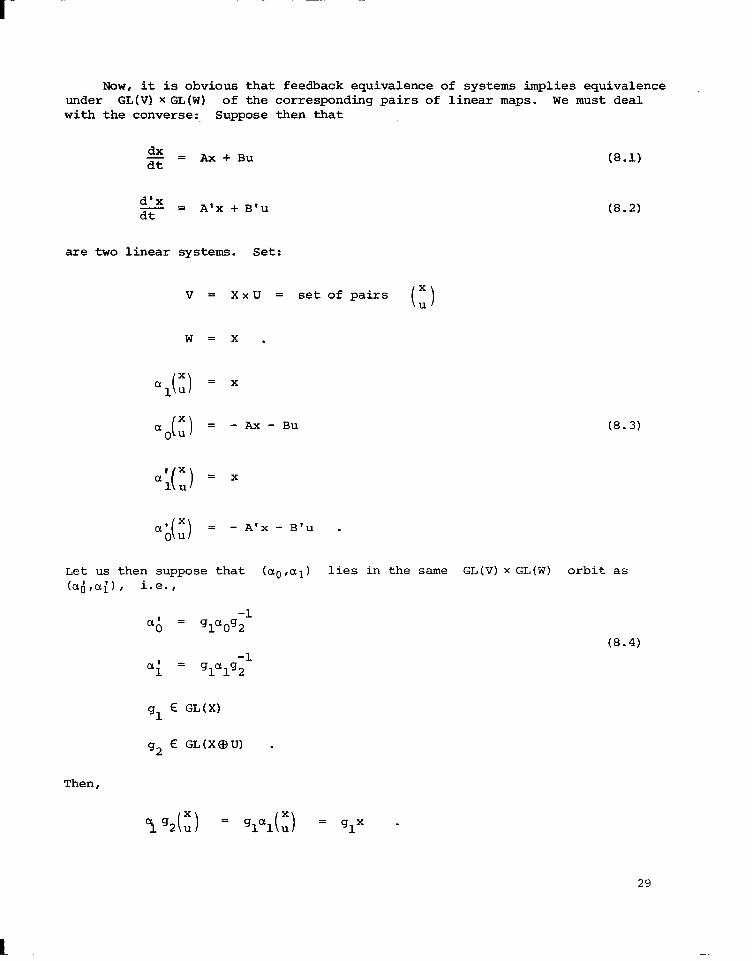
Now, it is obvious that feedback equivalence of systems implies equivalence under GL(V) XGL(W) of the corresponding pairs of linear maps. We must deal with the converse:, suppose then that
dx dt = Ax+Bu
d'x dt = A'x + B'u
are two linear systems. Set:
v = xxu = set of pairs
w=x.
= x
= -Ax-Bu
= x
= - A'x - B'u .
(8.1)
(8.2)
X ( 1 U
(8.3)
Let us then suppose that (a0 ,a11 lies in the same GL(V) x GL(W) orbit as (ad,ai), i.e.,
ai -1
= g1a0g2
(8.4)
*i
-1 = g1a1g2
g1 E GL(x)
g2 E GL(X@U) .
Then,
%92(Z) = glal(3 = glx -
29

Suppose g2 is written in partitioned form:
X
g2u = (
g2,11 g2,12
g2,21 g2,22 I() U
=
(
g2,11x+g2,12u
g2,21x+g2,22u )
g2 11 E L(X,X); ,
g2 12 E L(U,X) : I
g2 21 E L(X,U); g2 22 E L(U#U) . I I
Compare (8.5) and (8.6 :
12" = glx I
hence
1 41 = g2,11 1
1 42,12 = O 1
Plug (8.7) and (8.8) back into (8.4):
OK
(8.6)
(8.7)
(8.8)
a' 91X =
O 92 21x+g2 22"
- gl(Ax+Bu)
I I
or
30

A’glx + B’ (g2 21x+ g2 22u) I I = gl(Ax+Bu)
or
(8.9)
B’g 2,22 = glB (8.10)
These formulas can be summarized in the following way.
Theorem 8.1. The two input systems (8.1), (8.2) lead to GL(X) x GL(X $ U)- equivalent pairs of maps if and only if the systems differ by state feedback and by change of basis in input and state space. q
This result has two sorts of ramifications in system theory. First, it enables the state feedback classes to be classified by the Kronecker pen&Z theory. In fact, it was Brunovsky [ 51 who did this in a way independent of the general Kronecker theory. Second, it indicates a major algebraic difference between state feedback on the one hand and output feedback and various sorts of "compensators" on the other hand. If the latter sort define a group (which is not always clear), usually the orbits of these groups on systems are not equiva- lent to the problem Kronecker solved, i.e., equivalence of pairs of linear maps under isomorphisms of domain and range spaces. Problems of enumerating orbits are extremely difficult in our present state of knowledge of invariant theory if they do not reduce in one form or another to the Kronecker problem or are closely related to it. It is then a lucky accident (?) that state feedback is governed by the Kronecker invariant theory.
9. TRANSFER FUNCTIONS AND HOLOMORPHIC VECTOR BUNDLES FOR 1-D AND n-D SYSTEMS
The geometric methods introduced by Martin and me into system theory depend on associating with a finite dimensional, time-invariant input-output system a vector bundle on the Riemann sphere. Note that the Riemann sphere (the complex numbers with its one-point compactification) is the only Riemann surface of genus zero. This point of view is not really so avante-garde as it might sound, since it is very much in the spirit of the one-complex variable methods used by electrical engineers in the 1920's to '40s. (This is the material that was supplanted by "state space methods" in the late 1950's and 1960's.) We believe that there is considerable potential for applying these methods (enriched by
31

the modern,mathematical research) to more general systems. I will now develop material in this direction for systems described by ordinary and partial differ- ential equations.
There is a vast field of engineering practice called the "theory of two- dimensional filters", which as yet has no systematization and mathematization (as the "state space" theory systematized and mathematized one-dimensional filters). I believe the ideas presented here might put us on the road to such a theory. Another interesting possibility is an application of complex manifold methods to the systems of partial differential equations which occur in physics.
My plan is to try to construct holomorphic vector bundles with such systems. We shall see that this is a modern algebro-geometric version of the traditional "transfer function" methods used in system theory and electrical engineering.
Let us begin with well-known material. Consider a finite dimensional, linear, time-invariant input-output system
dx dt= Ax + Bu
Y =cx .
Convert this into an algebraic equation using the Laplace transform
co
ii(s) = I x(t)e -st dt 0
with zero initial conditions.
s;(s) = A;r + BG
or
$ = (C(s-A)-'B) ii
T(s) -1
= C(s-A). B
(9.1)
I
(9.2)
is the transfer function or frequency response. If U and Y are the linear input and output spaces, T is the natural mapping
9: -f L(U,Y) .
32

A more appropriate gadget from the Riemann surface is the sequence
'n = C(s-A) -lBsnds (9.3)
of differential forms. Let us see how they behave at s = m. Set:
1 U = -
S
du = - u2 ds
Bu-~u -2 du
= - C(l- Au) -1 -(n+l) du B u
= - C(l+Au+A2u2+ . . . ) B,J-(~+~) du - (9.4)
This shows that the Sn are meromorphic differential forms on the Riemann sphere. Their residue at u = 0, i.e., s = m, is especially important; it is the "Hankel data".
residue 9 = - CAnB . n
We are especially interested in the inverse Laplace transform
a+iw
s T(s)e st ds = a-ia
(9.6)
This formula describes the input-output relations in terms of objects which have an a priori meaning in terms of Riemann surfaces, the "Abelian Integrals"
It is a well-known and classical idea (in mathematics) that the appropriate way to generalize these ideas is to replace the Riemann sphere with other compact complex manifolds.
33
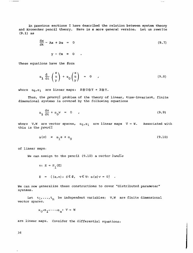
In previous sections I have described the relation between system theory and Kronecker pencil theory. Here is a more general version. Let us rewrite (9.1) as
dx dt-Ax+Bu = 0
Y -cx = 0 .
These equations have the form
alq;) +ao(;) = 0 I
(9.7)
(9.8)
where a0 #al are linear maps: XOUOY + X@Y.
Thus, the genera2 problem of the theory of linear, time-invariant, finite dimensional systems is covered by the following equations
'1 dt dv+aov = 0 I (9.9)
where V,W are vector spaces, co'al are linear maps v -+ w. Associated with this is the pencil
a(s) = 1 as+a 0 (9.10)
of linear maps.
We can assign to the pencil (9.10) a vector bundZe
IT: E + P,(c)
E = I(s,v): SEE, vEV: a(s)v = 01 .
We can now generalize these constructions to cover "distributed parameter" systems.
Let t1,...,t, be independent variables; V,W are finite dimensional vector spaces.
aoral' - - -fan: V + W
are linear maps. Consider the differential equations:
34
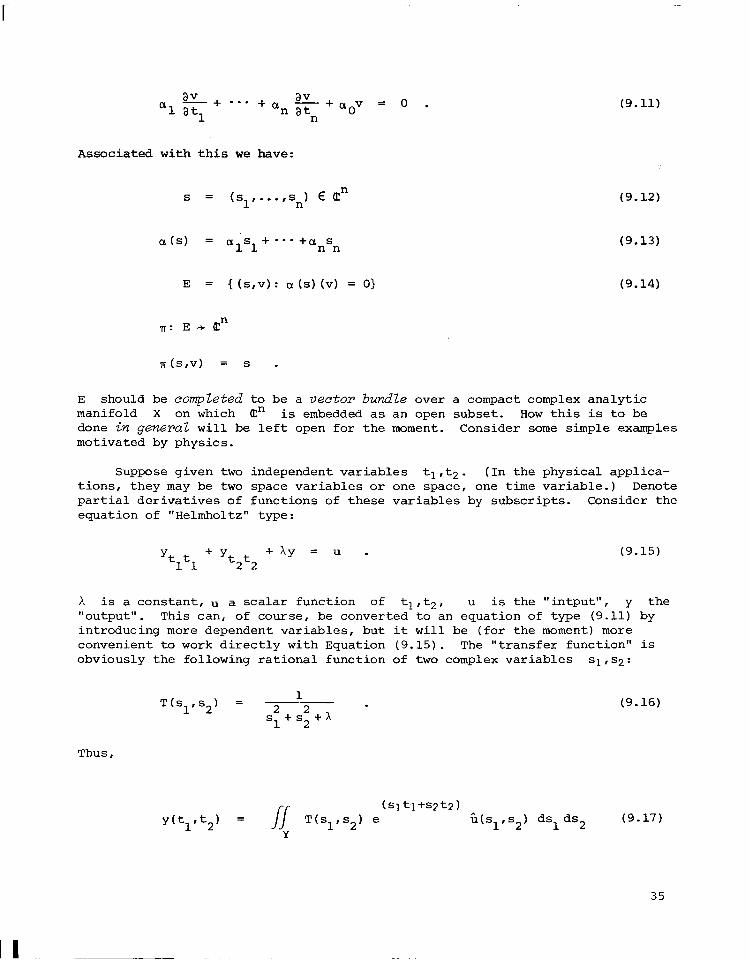
av
a1 at, -+ m-- +anE+aoV = 0 .
n
Associated with this we have:
S = (s 1 ,...,Sn) E an
a(S) = aiS + --- +anSn
E = { (S,V): a (S) (V) = 0)
(9.11)
(9.12)
(9.13)
(9.14)
TrTT(s,v) = s .
E should be completed to be a vector bundle over a compact complex analytic manifold X on which a:" is embedded as an open subset. How this is to be done in general will be left open for the moment. Consider some simple examples motivated by physics.
Suppose given two independent variables tl,t2. (In the physical applica- tions, they may be two space variables or one space, one time variable.) Denote partial derivatives of functions of these variables by subscripts. Consider the equation of "Helmholtz" type:
Yt t +Y +Ay = u . 11 t2t2
(9.15)
X is a constant, u a scalar function of tl,t2, u is the "intput", y the "Output". This can, of course, be converted to an equation of type (9.11) by introducing more dependent variables, but it will be (for the moment) more convenient to work directly with Equation (9.15). The "transfer function" is obviously the following rational function of two complex variables sll.59:
Tkl,s2) = 1
2 s1 + s; + h
. (9.16)
Thus,
JJ (s1t1+s2t2)
y(t1,t2) = T(sl,s2) e ;1(s p2) dsl ds2 (9.17) Y
35
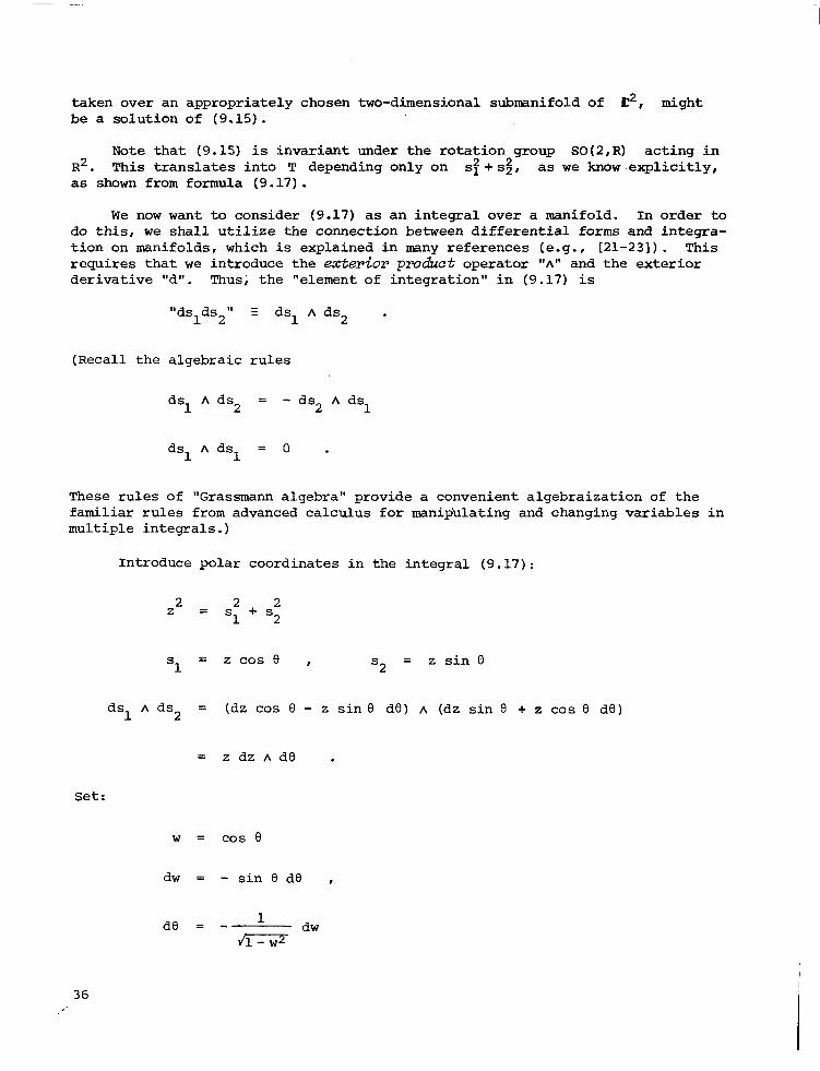
taken over an appropriately chosen two-dimensional submanifold of E2, might be a solution of (9.15).
Note that (9.15) is invariant under the rotation group SO(2,R) acting in R2. This translates into T depending Only on s~+s$, as we know explicitly, as shown from formula (9.17).
We now want to consider (9.17) as an integral over a manifold. In order to do this, we shall utilize the connection between differential forms and integra- tion on manifolds, which is explained in many references (e.g., 121-231). This requires that we introduce the exterior product operator "A" and the exterior derivative 'Id". Thus, the "element of integration" in (9.17) is
"dslds2" z dsl A ds2 .
(Recall the algebraic rules
dsl A ds2 = - ds2 A dsl
dsl A dsl = 0 .
These rules of "Grassmann algebra" provide a convenient algebraization of the familiar rules from advanced calculus for manip'ulating and changing variables in multiple integrals.)
Introduce polar coordinates in the integral (9.17):
z2 = s; + s;
s1 = z cos 0 , s2 = z sin 8
dsl A ds2 = (dz cos 8 - z sin 9 de) A (dz sin 8 + z cos 8 d8)
= zdzhde .
Set:
w = cos 6
dw = - sin 0 d8 ,
36

g.;..1..: (9.18)
Let us now suppose that u is a function of z alone. Then (9.17) can be rewritten as:
y(t1,t2) = z (tlw + t&-w2 )
e Q(z) Z
z2+E JiTz dw A dz
z(t1w + t2J1-w2) dw -- di=x
z;(z) dz z2+x
(9.19)
This formula exhibits the potential "algebra-geometric" nature of the situation. we have the algebraic correspondence
(s Its2 )+z = ,’
2 2 s1 + s2
(9.20)
of aG+Cl. (Note that is is not a "rational map". ) The fibers are the orbit of the orthogonal group SO(2,iT:). They are the circles
2 2 2 s1 + s2 = z1 .
In order to get a better idea of the algebro-geometric nature of the inte- grals (9.19), let us use a power series expansion for the exponential function. Set:
Y n,m = /-Jo (z J1-w2) m dldww2 & A;(Z) dz (g-21)
l-e.,
37

00 y(t1,t2) = x Y -
n,m=O nln2 n!m!
Thus, it might be appropriate to consider the
8 = n,m
(ZWP (z h-w2)m Jldw 2- --w
nm
e YS2 = n,m s; + s; + x
dslAds2
.
differential forms
Z A-
z2+ h
dz ,
(9.22)
(9.23)
(9.24)
as the characteristic "geometric objects" attached to the input-output system (9.15).
This suggests that we consider separately the differential forms
n (z J1-,2)" dw a
n,m = (zw) .
AC-Z- (9.25)
with z considered as a parameter. They are essentially differential forms on the Riemann surface whose local variable is w, i.e., the algebraic curve
2 2 w1 + w2 = 1 .
(A Riemann surface is a complex analytic manifold that can be parameterized by one complex variable. Of course, another point of view is to regard
z(t1w+ t,diGq dw e
l-w2
as a differential form on this Riemann surface. (Its indefinite integral can be written down explicitly in terms of Bessel functions.)
This simple example clearly gives us much new material to consider for a general theory of systems from a complex manifold-algebraic geometric point of view.
38

10. VECTOR BUNDLES ON ORBIT SPACES
We can immediately see a general pattern to the example treated in the previous section.
Let X,Y be spaces,
a map. Suppose given a vector bundle
IT:E'Y .
For yEY, the fiber E(y) = V'(y) is a vector space. It defines a vector bundle
4-l (El
on X, called the puZZ-back bundi!e
$-l(E) = ((x,v): v E E($(x))) .
There is a commutative diagram
6% ----+ E
Consider a given bundle E' on X andamap I$: X+Y. We can ask whether there is a bundle E on Y such that
E' = '$-l(E) .
One can also ask whether there is an equivalent vector bu.ndZe E" on a bundle E such that
E" = +-l(E) .
These questions are especially interesting for systems theorists (and physicists!) if the following additional structure is put on:
39

G is a transformation group on X. Y=G\X isthe orbit space, 4: X+G\X=Y the map which sends x E X into the orbit Gx on which it lies. G acts as a group of automorphisms of the vector bundle E'.
Let us return to the context of Section 9.
11. VECTOR BUNDLES DEFINED BY SYSTEMS OF PARTIAL DIFFERENTIAL EQUATIONS AND LINEAR
GROUPS OF SYMMETRIES
Let V,W be complex vector spaces, n an integer, and let ao,al,...,an: V + W be linear maps. We can then construct the system of linear crmstant coefficient partial equations:
av
a1at,+ --- +a "v-av = 0
n at 0 n (11.1)
to be solved for a function
t = +...,t,) -fv(t) ,
i.e., a map Rn -f V.
We can then associate with this system the n-complex variable "pencil"
a(s) = alsl+ -.- +ansn - a0 (11.2)
of linear maps: v -+ w, and the holomorphic vector bundle
n E = C(s,v): s = (s ,...,Sn) E& ; 1 a(s)v = 01 (11.3)
Now let G be a group. Suppose given three linear actions on CC:", V and W.
Definition. G acts as a syrrunetry group of the pencil a(s) if the follow- ing condition is satisfied:
ga (s)g -1
= a(g(s)).
for all g E G .
(11.4)
40

Such an action determines an action of G on the vector bundle E:
s(s,v) = (gs,sv) .
(If a(s)v = 0, note that using (11.4)
a(g(s)) (gv) = ga(s) (v) = 0 I
111.5)
so that the action (11.5) really does map E onto itself.)
Thus we can form the orbit space G\@ and ask whether the bundle E comes from a bundle on this orbit space. This is clearly an interesting system- theoretic way of defining vector bundles!
12. S0(3,&)-BUNDLES
If G has a known Lie-theoretic structure, we can use Lie group representa- tion theory to analyze the bundles constructed in Sectionll. One of the simplest cases (and the most important for physicists) is that where G is the three- dimensional rotation group. For algebraic reasons we complexify everything.
We are supposing that n = 3. Refer to [30] for notation and ideas used here. Thus, a0ralra2ra3 are linear maps: v+w. If
g(s) = gs E matrix multiplication .
It is convenient to write
a 3 (ala2a3)
s1 (a) 4s) 5 (a,a,a,) s2 + a0 . 0 s3
41

Suppose g is an orthogonal 3X 3 complex matrix, i.e.,
-1 g’=g .
(' denotes transpose of a matrix.) Let
al: G -+ L(V)
IS 2
: G + L(W)
be the given representations of G by linear transformations on V and W.
a2(g)(aks) ul(gol) = @(s(s))
or
-1 s1 5 a2 (g) (a1a2a3) al (g ) ( i s2 f 02(g)a0ul(g
-1 1 = (ala2a31g s2 + ao,
s3 ( i s3
or
u2(g)aOal(g -1
1 = a0
a2(g) (ala2a3)ul(g -1
1 = (a1a2a3)g .
Now,
L(V,W) E v @ wd -
(12.1)
(12.2)
(Wd = dual space to W. In fact, all finite dimensional representations of G are self-dual.) The "Clebsch-Gordan" rules for decomposition of tensor product representations of SO(3) tell how many such independent a's there are.
42

The irreducible (finite dimensional) representations of G are parameter- ized by an integer j ) 0 (E spin). The vector space for the spin j- representation has dimension (2j +l). Thus, V and W can be split up into a direct sum of vector spaces V.,W.
a in each of which G acts via a direct
sum of spin j-representations. s&g "Clebsch-Gordan" we see that
a(s)(Vj) C W. + W. + W. I+1 I 1-l
a (V.) C W. I 0 3 7
j = 0,1,2 ,... .
Example. Consider the Helmholtz operator with input u, output y;
2 sy+Ay-u = 0 .
Set:
x. = S.Y t 1 1
Thus,
c sixi = - Ay + u i=l
or
i=l,2,3 .
siy - xi = 0 , i = 1,2,3
c S.X. 11 +xy-u = 0 i
V = R5
x1
x2 = Ul x3
Y U
(12.3)
(12.4)
43

w = R4 .
i
x1
x2 (s) x3
Y u
SIY - x1
II I S2Y - 3
= S3Y - x3
c S.X. 11
+ xy - u i
(12.5)
Thus, we see that V is a direct sum of a spin one subspace S and two spin zero subspaces. W is the direct sum of an Sl and an SO. Now, Clebsch- Cordan gives:
%@ s1 = s2 CD s1 0 so
so 6 s1 = s1 ,
i.e., there are intertwining maps
It is these that are obviously present in (12.4).
13. THE COMPACTIFIED VECTOR BUNDLES DETERMINED BY THE HELMHOLTZ EQUATION
Continue with the situation of Sections 9-12, the linear differential equations which are invariant under the action of sO(3,iiZ:) on t3. These equations cover most of those of interest in classical mathematical physics! For s E ic3 let
E(s) = {v E V: a(s) (VI = 01 - (13.1)
As s varies over ES, E(s) defines a vector bundle whose basis is t3. G = SO(3,t:) acts linearly on E.
We want to examine the algebro-geometric structure of this bundle, and any possible bundles with orbit spaces
44

G\C3 .
The first step is to "homogenize" Equations (11.3), (12.4). homogeneous coordinates
Introduce
with
‘c. s.=‘,
1 i = 1,2,3
0
Equations (12.4) take the form
c TiY - X.T = 0
10
5 -ciXi + (Ay- U)To = 0 i=l
.
(13.2)
These equations determine a vector bundle E whose base is Pg(E:), which restricts to the given bwldle when &' is embedded as the 'affine" subspace of P3(C).
Let us work out the fibers of this bundle. If To # 0, these equations are equivalent to (11.3), and the solutions E(s) obviously form a one- dimensional vector space. The "input-output" relations are
1 I y=-u s2 + x
This gives a “geometric”, systems-theoretic meaning to 1/(9+X) as the "transfer-function-fundamental solution-Green's function" for the Helmholtz equation!
45

For
To = 0 I
Equations (13.2) take the following form:
T.X = 0 1
(13.3)
t:Tixi=o I i=l
Since one of the Ti is nonzero, (13.3) forces y = 0. Then, (13.3) reduces to
y = 0
5 TiXi = 0 i=l
(13.4)
E(T) consists of the (y,u,xi) such that only (13.4) is satisfied. Thus,
The vector bundle E does not have constant dimension as T ranges over P3(0I:). We see that there is here a distinct difference from the one-dimensional situation!
However, we can construct an equivalent bundle E' on t3 which does have a non-singular extension to P3(C) - Namely,
E’ =
1
1 (y,u,s): y = - u
s2+ h 1
.
Again, put
T. 1
S =- i TO
46

Thus,
1 E'(T) = (x,u): x = U
~~+x
'0
2 TO = (x,u): x = -
z T.T.
11 + +
Thus, if TO = 0,
E’ (~1 = I(x,u): x = 03 .
We see that for aZZ T E P3 (c:),
We can also examine how E' projects down to the orbit space SO(3,&) \a:". MaP
as follows
6 (s) = s2 = z .
The fibers are the orbits of SO(3,Q:). We would now like to "projectify" this situation
f.
se = 1
1 r.
z1 Z = -
=0
47

3 ‘$(Tc) = T;, c TiTi (13.5)
i=l
Note that this map sends one-dimensional linear subspaces of E4 into one- dimensional linear subspaces of C2, hence it passes to the equivalent to define a map
e: P3(Q) + Pi(Q) . (13.6)
The orbits of ~0(3,(c) lie in the fibers of 0.
Thus 4 and the vector bundle E' are very compatible.
2
E(T) = (x,u): x = TO U
c T.T ii + XT 2
i 0
Set:
E"((z ,d,)) = zO
(x,u): xsz +hz u - 10 I
This formula defines a non-singutar vector-bundle on Pl (a -
E' = $-l(E") ,
i.e., E' is the pull-back of the bundle on PI(E)-
14. LINEAR FILTERS AND GROUPS
So far, we have been considering the class of input-output systems defined in terms of differential equation,rrodels. of course, "system theory" is much more extensive, and not necessarily tied to all such models. In this section I will briefly describe another foundational approach. It too has a basic geometric aspect that has barely been developed.
Consider a "system" as a mapping from certain input data to certain output data. It is important to specify some sort of mathematical structure on the input-output data and to consider systems which interrelate this structure in
48

some way. For example, let us analyze the linear, finite dimensional, time- invariant state space models from this point of view. Consider one, say of the form
dx dt = Ax+BU
(14.1)
Y =cx .
XlU#Y are vectors in finite dimensional real vector space, and A,B,C are matrices of the appropriate size. t is a continuous time parameter. Let u: t -f u(t) be an input function. we can then solve (14.1) with zero initial Eon&&ions to define the output t + y(t):
t
y(t) = A(t-s) Bu(s) ds . (14.2)
We can then consider the system as a mapping _ U-+Y _ which is linear and of the form:
m
y(t) = / K(t,s) u(s) ds , -Cm
where (t,s) + K(t,s) is a mapping Rx R -t (matrices) such that the following ,conditions are satisfied:
a) K(t,s) = 0 if SC0 (14.4)
b) K(t,s) = 0.. if s > t, :r, (14.5) I __i .-a
cl K(t+$',s) = K(t,s-t'), h .rll t,t',s 6 R (14.6)
Condition '(14.4) is just a normalization of the output at t = 0, and is not particularly important. Condition (b) is crucial, since it expresses causality; if the incoming signal u is zero for time t< 0, it guarantees that the output x is also zero for t<ifi. Condition (14.6), which expresses translation invari- ance, is a group property, and suggests ,that group theory might be the appropriate general setting for some of these ideasc
For example, one might replace the role of the real numbers by the integers, Z. An input is then a map u: n + u(n) of Z space U), an output is a map y: Z -f (output-vector-space Y ), is a map
U-tY - -
of the form
R, i.e., set t -f (input vector
and the "system"
y(n) =.fi - K(n,m) u(m) .m=-co
(14.7)
49

We can immediately write down the analog of conditions (14.4)-C14.6). Such input-output relations might be generated by the difference equation analog of the differential equations (14.1):
xn+l = x n + Axn + Bu n (-14 -8)
Y n+l = cx n+l
However, we can generalize relation (-14.7) to other groups. For example, replace the integers Z with the direct product group zx z. A system then might be a map (input) + (output) of the form:
y(n,,n,) = C (yrm2)
K((y, 2 n ),(y, m2)u(ml,m2)) (14.9)
Relation (14.6) generalizes readily tothis case. However, the right generaliza- tion of (14.5)--causality--is less existent. In fact, there is now a large body of current engineering literature-lore concerning such systems, called, say, 2-D digita fiZters, and the lack of a natural generalization of "causality" is one complicating feature that has slowed down the development of a systematic theory paralleling the non-traditional 1-D theory. Of course, these non- traditional hybrid system-filter problems are extremely important in the state of today's technology, particularly in terms of realization of the ultimate potential of digital computers. Since I believe that geometric-group theoretic ideas are potentially important here also, I will now sketch a general setting for this approach. I will also indicate how some of the stochastic filter- system problems can be considered in the same way.
Suppose given the following data:
a) A real vector space U called the input space,
b) A real vector space Y called the output space,
cl A space T called the parameter\time-space.
U and Y may be infinite dimensional and T may be continuous or discrete. However, the functional analysis complications are reduced if we work with the case where T is discrete
d) A u-field of subsets of T, and a measure d-c on this sigma-field.
(In this section it will be assumed that the reader is familiar with the rudiments of measure theory and functional analysis, say at the level of Ref. [33].)
Let A--( T, Ul , A( TrYI denote the space of mappings with domain -C and range U and Y. A lineU2 System, in this framework, now might be defined as a triple (S, 8,X) with the following conditions satisfied:
a) .a = ck( T, U)
b) @c &I( T,Y)
cl 9 and @ are linear subspaces of the vector spaces in which they are embedded, by (a) and (b)
50

d) Lx is a linear map: 9 -+ @, of the following form:
s($ (T) = / K(T,T')u(T') dr' ,
T
(14.10)
where (T,-c') -t K(T,T') is a mapping of
TxT + (space of linear maps U-tY)
(Of course, one must also Pstulate sufficient functional analysis detail in order that the terms in (14.10) even make sense. In certain situations it is desirable to relax the framork to allow the "kernel" K to be a distribution- generalized function in the sense of L. Schwartz and F. Gelfand.)
In order to make contact between this general framework and contemporary engineering (and I want to emphasize how widely these ideas are dispersed throughout mathematics, statistics, and the signal-information-conununication- filtering-prediction parts of technology), it is of course necessary to special- ize further. There are two aspects I want to discuss briefly here because of their considerable geometric significance:
a) A group G acts on T as a transformation group, and certain relations of compatibility are presented between G and the system (9, 8,3iC). (The prototype is that where T = real numbers or integers, G = additive group, and the "compatibility" relations are those which describe "stationarity" of the processes.) The group action is denoted as
(g,r)-+gr -
b) G acts on the products TX U, TX Y, in the following way:
g(T ,U) = (gT,U(T,g) (U))
(14.11) g(r,y) = t.gTr8tT.g) (Y))
for T E T, g '2 G, u E u, y E Y.
We require that for each (T,g) I a(Trg) are linear maps on U and Y.
(Note that the conditions that (14.12) define a transformation group action on TXU and TXY requires that certain conditions be satisfied by a and B. We shall not write them down explicitly.)
This action (14.11) then defines an action of G on &(T,U) and &(T,Y), as follows:
(gU) (T) = U(T,g) ($g-‘T))
(14.12)
(sy) (.c) = 8(T,g) (x(g-‘T))
51

One can now require that systems, defined as linear maps
commute with the action of G on A(T,U) and d(T,Y) - This is a sort of generalized "stationarity". Here are some examples that appear with great frequency in the engineering literature.
Example. 2-D translation-invariant digital filters with scalar sigmZs.
Let U = Y = a:, the complex numbers, and let T= ZXZ, G = Zx Z acting on itself. Let G act on dd(T,U) and cM(T,Y) via simple translation:
Let K: T +
(gu) (n,,n,) = u((n,,n,) -9)
(14.13)
(gy) (n,,n,) = y((nl,n2) - 9)
for gE G 5 ZXZ, (n,,n,) E Zx Z .
P: be a map and let
S'Z: A(T,U) + &(T,Y)
be the map defined for the following,formula:
c43y) (n,,n,) = c K(nl - yI n2 - m2) (14.14)
(m l,m2) E ZXZ
This linear map x is translation invariant, i.e.,
Wgy) = gs4+) - (14.15)
Let us now exploit the invariance under G. Decompose .nl(T,U) into linear subspaces which transform irreducibly under G. This can be done in the following way: Let G* denote the set of all group-homomorphisms
TWO such homomorphisms can be multiplied; they form a group called the duaZ group to G. In this simple case (i.e., G=ZXZ), G" can be identified with ilzx CT: For z = (z ,z ) E ilzx c,
nlzi +n2z2 hz(nl,n2) = e . (14.16)
For A = z E G*, let uz 6 Jti((T,U) be the map defined as follows:
52

-nIzl-n2z2 zz(nltn2) = e
for (n,,n,) E T .
(14.17)
Thus, for g E G, X E G*,
du,) = XCg)ux (14.18)
This equation means that ux "transforms via the irreducible representation A".
The "digital filter" * now conunutes with G, linear subspace of &(T,Y) which transforms via A.
hence maps ux into a Set
-nlzl-n2z2 yz((nl,n2)) = e
Thus, for each h E z E (zl,z2) E E:xP: = G*,
X(yz) = ‘i’(zh~z
with f?(z) E t -
This function
(14.19)
z -+ IT(z) (14.20)
is called the transfer function of the filter/system s.
It can, of course, be computed in the more traditional way in terms of the kernel K.
.71(yz) (n,,n,) = C K(n -m hlrm2)
1 ltn2 -m,) yz(mlrm2)
= c K(nl-ml, n2 -m2) e-m1Z1-m2Z2
= c K(ml;m2) e -(nil+nl)zl+ (m2+n2)z2
= Yz(nlpn2) c Khl,m2) e -mlzl- "222
hence:
T(z) = xK(ml,m2) e -mlzI-m2z2
(14.21)
53

The right hand side of (14.21) is called (at least in the engineering literature) the z-transform of K.
The mathematical problems that are most important.for applications involve conditions for causality and stabiZity in terms of ?.
Example 2. Stationary stochastic process as inputs and outputs. This example is a traditional one in the engineering literature (and goes
back to the original work of Kolmogoroff and Wiener). First, let us review some probability theory.
Let R be a space with a fixed c-field of subsets and a probability measure dw defined on this family of subsets. A random variable is a measurable mapping f: Q+-R. The integral of f with respect to the probability measure du is called the expectation of f, and denoted as follows:
E(f) : / f dw (14.22) i-2
Let H denote the vector space of measurable functions f: fi -f R such that
E(f2) : f2 dw < 00 (14.23)
H then forms a HiZbert space--"the" L2 of dw. The inner product is
(fl’f2) + <f lJf2> - E(flf2) .
The norm is
Ml - <f,f>li2
Let T again denote a parameter space. (It will suffice to suppose T discrete. This avoids certain analytic complications of the theory of stochastic processes.) For our purposes, it suffices to restrict attention to random variables that are square-integrable, i.e., lie in H. A stochastic process (parameterized by T) is a mapping
S:T+H .
Suppose such a process S is given, and in addition, G is a transformation group on T. Let O(H) be the group of isomorphisms of the Hilbert space H, l.e., the space of linear maps A:H+H such that:
54

The inverse map A -1 exists
<Ahl,Ah2> = <hl,h2 >
l-e., A is isometric .
Definition. The stochastic process S: T -f H is S&ationuPy (relative to group G which acts on T) if there is a group-homomorphism CL: G + O(H) such that
a(g) (s(T) 1 -1
= S(g T) (14.24)
for gEG, TET .
Remark. Condition (14.24) means that the "means" and "correlations"
T -+ E(S(r))
(TlrT2) -f E(S(T~)S(T~)
are invariant under transZation by G. In the case where T=R or Z, G= additive group of translations, this is what is usually called "weak stationarity" in the theory of stochastic processes.
Having defined "stationary processes" in this way, we may now define filters as maps whose domain and range are stationary stochastic processes. For example. if T = G = Z, it is readily seen that such linear filters are of the form
f + k*f,
where k:T+R is a real-valued function and * is the usual convolution. Again, as in Example 1, this leads us back to "harmonic analysis" of the group G.
In summary, in this section we have briefly seen that there are possibili- ties for application of general Lie group-geometric methods in the theory of deterministic and stochastic filters.
150 CONCLUDING REMARKS
Certain general principles for the application of modern differential geometry to system theory have been presented. These principles have been applied (in joint work with Clyde Martin) to the feedback structure of linear time-invariant systems. bundles.
The key technique is the theory of holomorphic vector Such bundles can also be defined for distributed parameter systems,
although they now have singularities and their "poles" become submanifolds.
55

This approach constructs a bridge between the classical work in electrical . engineering and control theory concerned with the description of systems via
t'transfer functions" and modern differential and algebraic geometry. Where the engineer speaks of "poles", the geometer considers "intersections". One might expect that mathematics of this sort will become essential for a systematic treatment of the "non-classical" control problems that are on the technological horizon.
56

APPENDIX GENERALIZATION OF THE PSEUDO-INVERSE CONSTRUCTION TO
RIEMANNIAN MANIFOLDS; SLICES AND CANONICAL FORMS FOR GROUP ACTIONS
One of the fundamental mathematical problems of system theory is to find liftings of mappings in the following sense:
Let X,Y,A be spaces and let
IT: x+Y
I$: A-+Y
be mappings. We want to find mappings
I$’ : h-+x ,
such that
I@’ (Xl = 9(X)
for all X E A .
Further, one wants to let 4' depend on 4 in a reasonably "robust" way.
For example, the estimation problem takes this form:
X = a space of systems
Y = a space of input-output relations
IT: X-+Y the map which assigns to each system the input- output relations it determines .
In case X is the space of controllable and observable linear systems with given input, state, and output spaces, Y is the orbit space of the action of the group of change of bases on state space.
In case X and Y are finite dimensional vector spaces, the construction of 4' is usually handled via what is called (in statistics and numerical analysis) the pseudo-inverse. We shall first recall its definition, then sketch a possible generalization to Riemannian manifolds. Then 'we go on to the case (which has evident implications for system theory) where Y is the orbit space of the action of a group G on X. The simplest general theory occurs when X has a Riemannian metric, and G is a group of isometrics of this Riemannian
57

-
metric. In case G is discrete, Poincare suggested (in classical work) a method of constructing a "fundamental domain", i.e., a slice of the orbit space. In l311, the author has suggested a method of generalization of Poincard's construction. This construction will be reviewed in this appendix.
The Pseudo-Inverse
Suppose that X and Y are finite dimensional real vector spaces with a given positive-definite synmetric dot product:
(x,x)+x 12 1 l x 2ER
(Y,,Y,) + yl- y2 E R -
The iwrms of x and y are then
IIXII = (x l x)1’2
IlYll = (Y l YF2
d(xl,x2) = lb3 -x211
d(ylry2) = llY1-Y211
are then metrics on X and Y.
Suppose that Tr: X-tY is a linear map. Let IT*: Y-+X bethedualmzp, defined by the following relation
y - TX = a*y 9 x
for x E x, yEY .
Let us now minimize the function x + 11412~ subject to the constraint Y -lrx = 0. Using the Lagrange multiplier rule, introduce the Lagrange multi- plier vector A E Y and define the function
f(X,Y,X) = ]lxl12 + x * (Y-W
We now look for the unconstrained critical points of the function x + f(X,Y,A) with (y,X) held fixed:
58

k f(x+tsx,y,A) = 2x* 6x-21 l lT(bx)
t=o
= 2(x-IT*(h)) - 6x .
X is a critical point of this function if and only if
X = IT*(X) . (A-1)
The constraint condition gives:
Y = mr*(A) . (A.21
Definition. The pseudo-inverses of y under the map IT are the points x E X of the form (A-l), where X E Y satisfies (A-2).
Remark. Notice that conditions (A-1) and (A.2) together imply that TX = y* There is a pseudo-inverse if and only if TTTT* is an isomorphism Y+Y. In this case,
y + a*(TrlT*) -l(y) z Y(Y)
is a map Y + X which is a cross-section of the map 7r: X + Y, i.e., Try = identity.
Maps Between Riemannian Manifolds
Let X and Y be Riemannian manifolds. Denote the inner product on tangent vectors as
(yv,) -+ <v1,v2 > .
(For notation or background of Riemannian geometry, see 1221.) If t + x(t), a<t<b, is a curve in X, then - -
b
J( dx dx l/2 -I dt dt >
dt a
is the length of the curve. The distance d(xl,xp) between two points x1rq E x is the greatest lower bound of the length of all continuous, precise Cm curves joining x1 to x2. This satisfies all the usual axioms needed to define a metric space.
59

Suppose that T: X -t Y is a map. Pick a point x0 E X which is held fixed throughout the discussion. If 2 is a subset of X, let
d(xOA = inf d(xD,z) . ZEZ
For y E Y, set
Y(Y) = {xEX: XEIT-l(y), and d(xO,x) E d(xG, n-'(y))}
The points in Y(Y) are called the pseudo-inverses of x under the map IT (relative to the fixed Riemannian metric).
We are especially interested in three questions:
a) When do there exist points in Y(Y)?
b) When does there exist a unique point in y(y)?
cl If there is a unique point in Y(Y) for each y E Y, is the map y+y(y) of Y-+X (which is a cross-section for the map IT: X -f Y) sufficiently smooth to provide the sort of "robust" liftings of mappings h-+Y needed for applications?
Now, a reasonable sufficient condition for (a) is the following one:
a’) The subset m-l(y) is a closed, regularly embedded submanifold of X and the Riemannian metric on X is complete.
In case (a') is satisfied, and x0 lies sufficiently near s-l(x) (e.g., in a tubular neighborhood), then (b) will be satisfied. However, there is no known reasonable condition which will imply (b). (c) represents even more unknown territory. However, the powerful techniques available for handling questions like these ("global Riemannian geometry") give some hope that this is a construction which might prove useful in certain circumstances. Certainly, it is the natural generalization of the "pseudo-inverse", which has proved to be widely useful and deserves further study. To my knowledge, there is no work in the literature in this direction.
SLICES, FUNDAMENTAL DOMAINS, CANONICAL FORMS, ETC. FOR TRANSFORMATION GROUP ACTIONS
Let X be a manifold, G a Lie group, and GXX-t X: (grx) + gxr be a transformation group action on X. The orbits of G are the subsets of x of the form Gx, with x E x. An orbit space for G acting on X is another space Y (possibly having a more general structure than a manifold) and a map TI: x+Y such that the fibers a-l(y), for yEY, are the orbits of G. Suppose such an orbit space is given.
60

A subset s c x is a slice (or fundumentaZ domain) for the action of G if s meets each orbit of G in precisely one point, i.e., if the following condition is satisfied:
IT restricted to S is one-one and onto.
Thus, if y = (-IT restricted to s)-l, y is a cross-section map: Y + x. (Conversely, if y: Y -+ X is a cross-section map for 'TI, then s = y(y) is a slice.)
One usually wants S to have further properties. For example, it would be nice if it were a submanifold. (This is usually too much to hope for.)
The concept of wcanonical form" is rather vague and indeterminate in the literature. Sometimes it means a slice, sometimes a more general subset which touches the "generic" orbit in precisely one point, but may have a larger inter- section with certain "singular" orbits. In system theory (where it is the key concept in attempts to solve the "identification problem") it is often a sub- manifoZd of x, which touches a "generic" set of orbits precisely once, but does not necessarily touch all orbits.
In one case, generalizing the classical construction due to Poincare for discrete groups [31], there is an elegant and useful definition of a "slice". Namely, suppose that X is a complete connected Riemannian manifold, and that G is a group of isometiies of X which is a closed subgroup of the Lie group of all isometries of X. It follows 1221 that all orbits of G are regularly embedded, closed submanifolds of X, and that each has a tubular neighborhood which is invariant under G. Pick a point x0 E x. Set:
P = IxEX: d(x,xJ (d(xD,Gx)] .
The proof that P is a slice, and has other nice properties, is given in [22], which also contains further useful general information about the orbits and the structure of the orbit space in this case. Finally, notice that P is precisely the "generalized inverse" set, as defined above, where Y = orbit space G\& and Tr: X-+Y is the natural quotient map which assigns the orbit Gx to each x E x.
REFERENCES
1. J. Willems, "Topological Classification and Structural Stability of Linear Systems", preprint, Groningen UniVerSity, 1977.
2. R. Hermann, Geometry, Physics and Systems, Marcel Dekker, 1973.
3. R. Hermann, "On the Accessibility Problem of Control Theory", Proc. Symp. On tiffePe?haZ Equations, A.J. Lasalle and S. Lefschetz (eds.), Academic Press, 1967.
61
4.
5.
6. F. Gantmacher, Matrix Theory, Chelsea, New York, 1964.
7. R. Hermann, "Interdisciplinary Mathematics", Vol. 9, Math Sci Press, Brookline, MA, 1975.
8. M. Hazewinkel, "Representation of Quivers and Moduli of Linear Dynamical Systems", 7976 Ames Research Center (NASA) Conf. on Geometric Control Theory, C. Martin and R. Hermann teds.), "Lie Groups: History, Frontiers and Applications", Vol. 7, Math Sci Press, Brookline, MA, 1977.
9.
10.
11.
12.
13.
14.
15.
16. B-D-0. Anderson and J. Moore, Linear Optimal Control, Prentice-Hall, 1971.
17. R. Brockett, Finite Dimensional Linear Systems, Wiley, 1970.
18. Rosenbrock, Multivariable and State Space Theory, Nelson, Iondon, 1970.
19.
20.
M. Wonham, Linear Multivariable Control, Springer-Verlag, 1974.
W. Boothby, An Introduction to Differentiable Manifolds and Riemannian Geometry, Academic Press, 1975.
21.
22.
R. Hermann and A. Krener, "Nonlinear Controllability and Observability", IEEE Trans. Aut. Cont. AC-22 (1977), 728-740.
P. Brunovsky, "A Classification of Linear Controllable Systems", Kybenetika 2 (1970), 173-187.
C. Martin and R. Hermann, "Applications of Algebraic Geometry to Systems Theory", SIAM J. Control and Opt. 16 (1978), 743-755. -
D. Husemoller, Fiber Bundles, Springer-Verlag, 1972.
J. Milnor and J. Stasheff, Characteristic Classes, Princeton Univ. Press, Princeton, NJ, 1970.
A. Grothendieck, Am. J. Math. 79 (1957), 121-138. -
R. Hermann, "Remarks on the Geometry of Systems", Proc. Nato Institute on Geometric and Algebraic Methods for Nonlinear Systems, R. Brockett and D. Mayne (eds.), D. Reidel, 1973.
R. Hermann and C. Martin, "Applications of Algebraic Geometry to Systems Theory", Parts 5 and 6, in Proc. 1976 Ames Research Center Conf. on Geometric Control Theory, Math Sci Press, Brookline, MA, 1977.
M. Hazewinkel, 'Degenerating Families of Linear Dynamical Systems, I', Proc. 1977 IEEE Conf. on Decision and Control.
J. Dieudonng, Treatise on Analysis, vol. 4, Academic Press, 1974.
R. Hermann, Differential Geometry and the Calculus of Variations, 2nd Edition, Math Sci Press, Brookline, MA, 1978.
62
23.
24.
25.
26.
27.
28.
29.
30.
31.
32.
33.
P. Griffiths and J. Harris, Principles of Algebraic Geometry, Wiley, 1978.
A. Feuer and S. Morse, "Adaptive Control of Single Input-Output Linear Systems", IEEE Trans. Au-t. Control. AC-23 (1978), 557-570.
G. Goodwin, P. Ramadge, and P. Caines, "Discrete Time Multivariable Adaptive Control (to appear).
R. Hermann and C. Martin, "Applications of Algebraic Geometry to System Theory", Part I, IEEE Trans. Auto. Control, AC-22 (1977), 19-25.
C. Byrnes and N. Hurt, On the Moduli of Linear Dynatical Systems, Studies in AnaZysis (Advances in Mathematics Supplementary Studies), Academic Press, 1979.
R. Brockett, "Some Geometric Questions in the Theory of Linear Systems", IEEE Trans. Auto. Control, AC-21 (1976)
R. Brockett and P. Krisnaprasad, "Scaling Rational Functions and Linear System Identification", to appear.
R. Hermann, Lectures on Mathematical Physics, Vol. 2, W.A. Benjamin, Reading, MA, 1972.
R. Hermann, "On the Existence of Fundamental Domains for Riemannian Transformation Groups", Proc. Amer. Math. Sot. 13 (1962), 489-494. -
R. Hermann, Vector Bundles in Mathematical Physics, Parts I & II, W.A. Benjamin, Reading, MA, 1970.
M. Davis, Linear Estinmtion and Stochastic Control, Chapman and Hall, London, 1977.
63
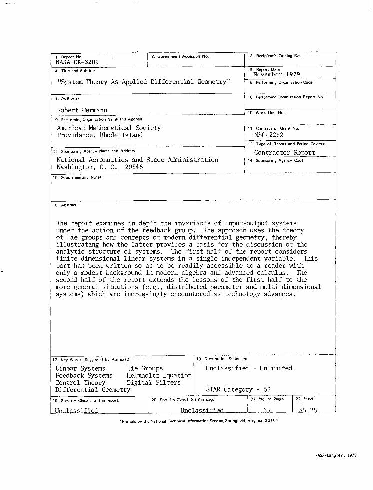
--- 1. Report No. 2. Government Accession No. 3. Recipient’s Catalog No.
NASA CR-3209 4. Title and Subtitle 5. Report Date
November 1979 "System Theory As Applied Differential Geometry" 6. Performing Organization Code
7. Author(s)
Robert Hermann -- 9. Performing Organization Name and Address
American Mathematical Society Providence, Rhode Island
2. Sponsoring Agency Name and Address
National Aeronautics and Space Administration Washington, D. C. 20546
5. Supplementary Notes
10. Work Unit No.
11. Contract or Grant No.
NSG-2252 13. Type of Report and Period Covered
Contractor Report 14. Sponsoring Agency Code
6. Abstract
The report examines in depth the invariants of input-output systems under the action of the feedback group. The approach uses the theory of Lie groups and concepts of modern differential geometry, thereby illustrating how the latter provides a basis for the discussion of the analytic structure of systems. The first half of the report considers finite dimensional linear systems in a single independent variable. This part has been written so as to be readily accessible to a reader with only a modest background in modern algebra and advanced calculus. The second half of the report extends the lessons of the first half to the more general situations (e.g., distributed parameter and multi-dimensional systems) which are increasingly encountered as technology advances.
7. Key Words (Suggsted by Author(s))
Linear Systems Lie Groups Feedback Systems Helmholtz Equation Control Theory Digital Filters Differential Geometry 9. Security Cl&t. lot this reportI 20. Security Classif. 1
18. Distribution Statement
Unclassified - Unlimited
STAR Category - 63 this page) ~-~ l<;%%r
. . lUnclass7lI s.7.s ‘For sale by the National Technics1 Information Sewce. Springfield. Virglnla 22161
Unclassified
NASA-Langley, 1979