SVMsCS446 Fall ’14 1 (recap) Kernel Perceptron. SVMsCS446 Fall ’14 2 (recap) Kernel Perceptron

SVMs CS446 Fall ’14 1

)(x yr w w,y)f(x If (k)(k)(k)(k) t

t(x))sgn(w))t(xwsgn( f(x) :function DecisionR w:Hypothesis

Rt(x) t(x),x : mapping Nonlinear ;{0,1} x :Examples

i

n'

1i in'

n'n

;

If n’ is large, we cannot represent w explicitly. However, the weight vector w can be written as a linear combination of examples:

Where is the number of mistakes made on Then we can compute f(x) based on and

(recap) Kernel Perceptron

)),(

m

1j

(j)(j)j

m

1j

(j)(j)j xxyrsgn(t(x)))t(xyrsgn( t(x))sgn(w f(x) K

m

1j

(j)(j)j t(xyr w )


In the training phase, we initialize to be an all-zeros vector.For training sample instead of using the original Perceptron update rule in the space

we maintain by

based on the relationship between and :


t(x))sgn(w f(x) :function DecisionR w:Hypothesis

Rt(x) t(x),x : mapping Nonlinear ;{0,1} x :Examplesn'

n'n

;

(recap) Kernel Perceptron

m

1j

(j)(j)j t(xyr w )

1)),(

kk(k)

m

1j

(k)(j)(j)j

(k) then yxxyrsgn( )f(x if K


Data Dependent VC dimensionConsider the class of linear functions that separate the data S with margin °. Note that although both classifiers (w’s) separate the data, they do it with a different margin.

Intuitively, we can agree that: Large Margin Small VC dimension


Generalization


Margin of a Separating HyperplaneA separating hyperplane: wT x+b = 0

Assumption: data is linear separableDistance between wT x+b = +1 and -1 is 2 / ||w||Idea: 1. Consider all possible w

with different angles2. Scale w such that the

constraints are tight3. Pick the one with largest

margin

wT x+b = 0wT x+b = 1

wT x+b = -1

wT xi +b¸ 1 if yi = 1wT xi +b· -1 if yi = -1

=>


Maximal Margin

The margin of a linear separatorwT x+b = 0is 2 / ||w||

max 2 / ||w|| = min ||w|| = min ½ wTw

s.t


Margin and VC dimensionTheorem (Vapnik): If H° is the space of all linear classifiers in <n that separate the training data with margin at least °, then

VC(H°) · R2/°2

where R is the radius of the smallest sphere (in <n) that contains the data.This is the first observation that will lead to an algorithmic approach.The second observation is that:

Small ||w|| Large MarginConsequently: the algorithm will be: from among all those w’s that agree with the data, find the one with the minimal size ||w||


Hard SVM OptimizationWe have shown that the sought after weight vector w is the solution of the following optimization problem:

SVM Optimization: (***)

This is an optimization problem in (n+1) variables, with |S|=m inequality constraints.

s.t


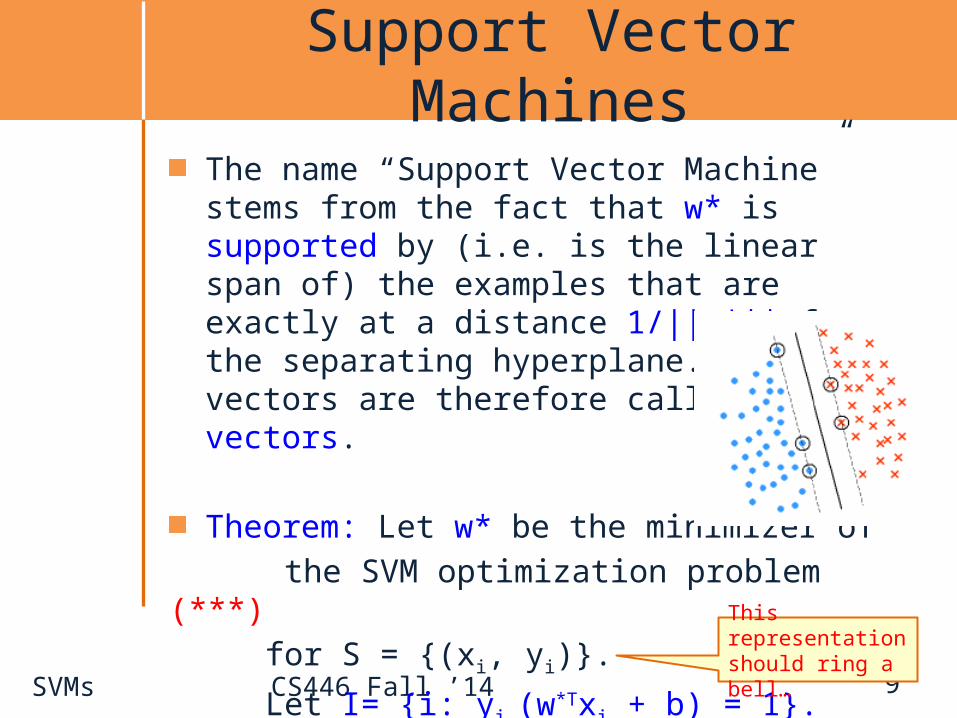
Support Vector Machines

The name “Support Vector Machine” stems from the fact that w* is supported by (i.e. is the linear span of) the examples that are exactly at a distance 1/||w*|| from the separating hyperplane. These vectors are therefore called support vectors.

Theorem: Let w* be the minimizer of the SVM optimization problem (***) for S = {(xi, yi)}.

Let I= {i: yi (w*Txi + b) = 1}.

Then there exists coefficients ®i > 0 such that:

w* = i 2 I ®i yi xiThis representation should ring a bell…



t(x))sgn(w))t(xwsgn( f(x) :function DecisionR w:Hypothesis

Rt(x) t(x),x : mapping Nonlinear ;{0,1} x :Examples

i

n'

1i in'

n'n

;

If n’ is large, we cannot represent w explicitly. However, the weight vector w can be written as a linear combination of examples:

Where is the number of mistakes made on Then we can compute f(x) based on and

Recap: Perceptron in Dual Rep.

)),(

m

1j

(j)(j)j

m

1j

(j)(j)j xxyrsgn(t(x)))t(xyrsgn( t(x))sgn(w f(x) K

m

1j

(j)(j)j t(xyr w )


Duality

This, and other properties of Support Vector Machines are shown by moving to the dual problem.

Theorem: Let w* be the minimizer of the SVM optimization problem (***) for S = {(xi, yi)}.

Let I= {i: yi (w*Txi +b)= 1}.

Then there exists coefficients ®i >0

such that: w* = i 2 I ®i yi xi


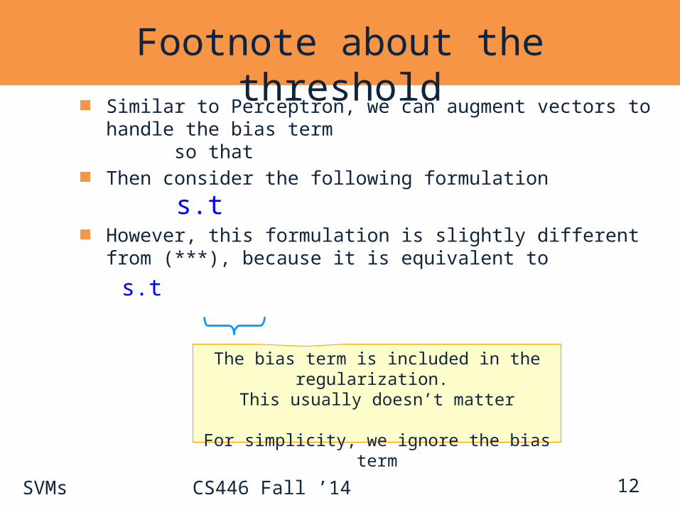
Footnote about the thresholdSimilar to Perceptron, we can augment vectors to handle the bias term

so that Then consider the following formulation

s.tHowever, this formulation is slightly different from (***), because it is equivalent to

s.t

The bias term is included in the regularization. This usually doesn’t matter

For simplicity, we ignore the bias term


Key Issues

Computational Issues Training of an SVM used to be is very time consuming – solving

quadratic program. Modern methods are based on Stochastic Gradient Descent and

Coordinate Descent.

Is it really optimal? Is the objective function we are optimizing the “right” one?


Real Data 17,000 dimensional context sensitive spelling Histogram of distance of points from the hyperplane

In practice, even in the separable case, we may not want to depend on the points closest to the hyperplane but rather on the distribution of the distance. If only a few are close, maybe we can dismiss them.

This applies both to generalization bounds and to the algorithm.


Soft SVM

Notice that the relaxation of the constraint: Can be done by introducing a slack variable (per example) and requiring: Now, we want to solve:

s.t


Soft SVM (2)

Now, we want to solve:

Which can be written as:

What is the interpretation of this?

s.t

In optimum,

s.t


Soft SVM (3)

The hard SVM formulation assumes linearly separable data.A natural relaxation: maximize the margin while minimizing the # of examples that violate the margin (separability) constraints. However, this leads to non-convex problem that is hard to solve. Instead, move to a surrogate loss function that is convex. SVM relies on the hinge loss function (note that the dual formulation can give some intuition for that too).

Minw ½ ||w||2 + C (x,y) 2 S max(0, 1 – y wTx)

where the parameter C controls the tradeoff between large margin (small ||w||) and small hinge-loss.

SVMs CS446 Fall ’14

SVM Objective Function

18

A more general framework SVM: Minw ½ ||w||2 + C (x,y) 2 S max(0, 1 – y wTx)

General Form of a learning algorithm: Minimize empirical loss, and Regularize (to avoid over fitting) Think about the implication of large C and small C Theoretically motivated improvement over the original algorithm we’ve see at

the beginning of the semester.

Can be replaced by other loss functionsCan be replaced by other regularization functions

Empirical lossRegularization term


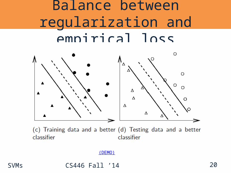
Balance between regularization and empirical loss


Balance between regularization and empirical loss

(DEMO)

http://www.csie.ntu.edu.tw/~cjlin/libsvm/js-toy/example.html



Underfitting Overfitting

Model complexity

ExpectedError

Underfitting and Overfitting

Simple models: High bias and low variance

Variance

Bias

Complex models: High variance and low bias

Smaller C Larger C


What Do We Optimize?


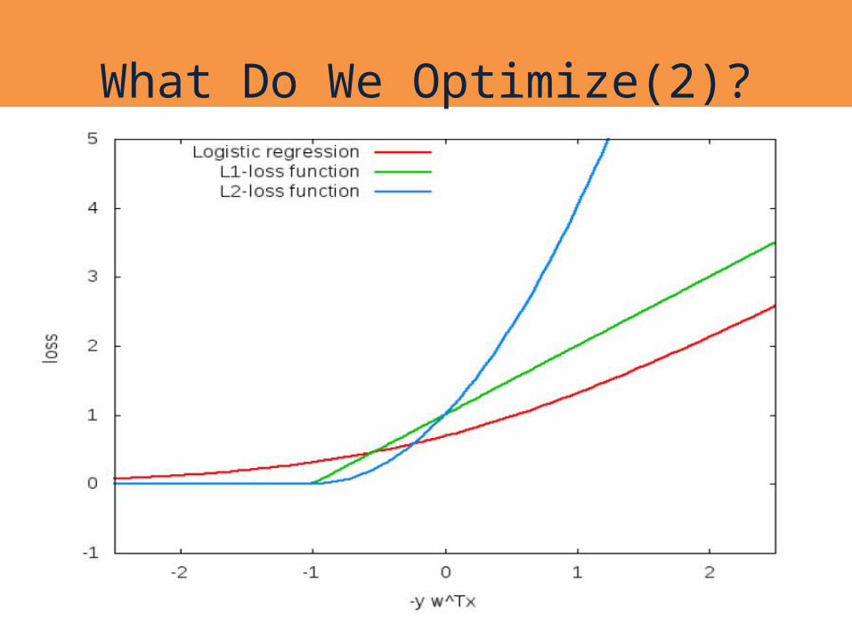
What Do We Optimize(2)?We get an unconstrained problem. We can use the gradient descent algorithm! However, it is quite slow.Many other methods Iterative scaling; non-linear conjugate gradient; quasi-Newton

methods; truncated Newton methods; trust-region newton method. All methods are iterative methods, that generate a sequence wk that

converges to the optimal solution of the optimization problem above.

Currently: Limited memory BFGS is very popular


Optimization: How to Solve1. Earlier methods used Quadratic Programming. Very slow.2. The soft SVM problem is an unconstrained optimization problems. It is possible to use the gradient descent algorithm! Still, it is quite slow.Many options within this category: Iterative scaling; non-linear conjugate gradient; quasi-Newton methods;

truncated Newton methods; trust-region newton method. All methods are iterative methods, that generate a sequence wk that

converges to the optimal solution of the optimization problem above. Currently: Limited memory BFGS is very popular

3. 3rd generation algorithms are based on Stochastic Gradient Decent The runtime does not depend on n=#(examples); advantage when n is very large. Stopping criteria is a problem: method tends to be too aggressive at the beginning and

reaches a moderate accuracy quite fast, but it’s convergence becomes slow if we are interested in more accurate solutions.

4. Dual Coordinated Descent (& Stochastic Version)


SGD for SVMGoal: m: data size

Compute sub-gradient of if ; otherwise

1. Initialize

2. For every example

If update the weight vector to

( - learning rate)

Otherwise

3. Continue until convergence is achieved

This algorithm should ring a bell…

Convergence can be proved for a slightly complicated version of SGD (e.g, Pegasos)

m is here for mathematical correctness, it doesn’t matter in the view of modeling.


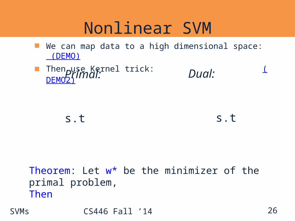
Nonlinear SVMWe can map data to a high dimensional space: (DEMO)Then use Kernel trick: (DEMO2)Primal:

s.t

Dual: s.t

Theorem: Let w* be the minimizer of the primal problem, Then

http://www.csie.ntu.edu.tw/~cjlin/libsvmtools/svmtoy3d/examples/




Nonlinear SVM

Tradeoff between training time and accuracyComplex model v.s. simple model

From: http://www.csie.ntu.edu.tw/~cjlin/papers/lowpoly_journal.pdf

Documents

SVMsCS446 Fall ’14 1 (recap) Kernel Perceptron. SVMsCS446 Fall ’14 2 (recap) Kernel Perceptron