SVM by Sequential Minimal

Optimization (SMO)    

www.cs.wisc.edu/~dpage  

1  

Quick  Review  

As  last  lecture  showed  us,  we  can  – Solve  the  dual  more  efficiently  (fewer  unknowns)  – Add  parameter  C  to  allow  some  misclassificaAons  – Replace  xiTxj  by  more  more  general  kernel  term  

2  

IntuiAve  IntroducAon  to  SMO  

•  Perceptron  learning  algorithm  is  essenAally  doing  same  thing  –  find  a  linear  separator  by  adjusAng  weights  on  misclassified  examples  

•  Unlike  perceptron,  SMO  has  to  maintain  sum  over  examples  of  example  weight  Ames  example  label  

•  Therefore,  when  SMO  adjusts  weight  of  one  example,  it  must  also  adjust  weight  of  another  

3  

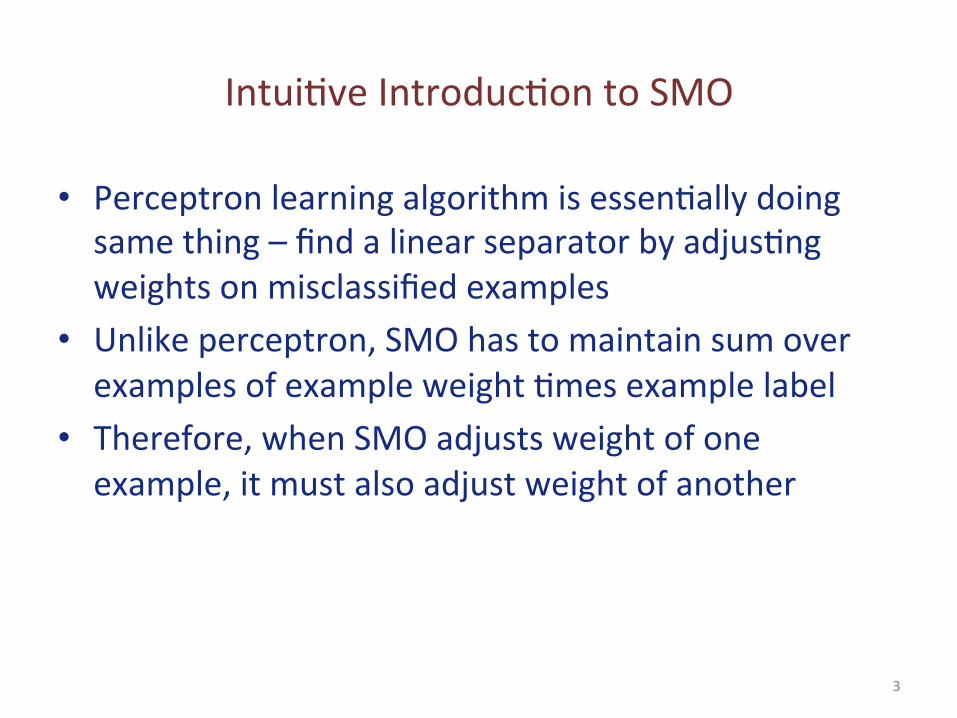
IntuiAve  IntroducAon  to  SMO  

w1

(w1 ,w2,...,wN ) =α1 (x11, x

12,..., x

1N )+α2 (x

21, x

22,..., x

2N )+...+αM (x

M1, x

M2,..., x

MN )

•  Can  view  weight  vector  for  perceptron  as  weighted  sum  of  examples:  

 

•  Learning:  Repeat  unAl  convergence  property  met  – Randomly  choose  an  example  –  If  mislabeled,  add  to  its  weight    

•  SMO  does  same,  except  must  respect  constraint:  

αi y(i)

i=1

m

∑ = 04  

IntuiAve  Intro  (ConAnued)  

•  This  constraint  means  whenever  we  add  an  amount  β  to  an  αi  ,  we  have  to  either:  – subtract  β  from  the  αj  for  another  example  with  the  same  sign  (class  label),  or  

– add  β  to  the  αj  for  another  example  with  the  opposite  sign  (class  label)  

•  Therefore  at  each  step  we  have  to  randomly  choose  two  examples  whose  weights  to  revise,  and  size  of  revision  depends  on  difference  in  their  errors  

•  For  soW  margin  SVM,  we  also  have  to  “clip”  size  of  any  change  because  of  addiAonal  constraint  that  every  α  must  be  between  0  and  C  

5  

Recall  Perceptron  as  Classifier  

•  Output  for  example  x  is  sign(wTx)  •  Candidate  Hypotheses:  real-­‐valued  weight  vectors  w  •  Training:  Update  w  for  each  misclassified  example  x  (target  

class  y,  predicted  o)  by:  –  wi        wi  +  η(y-­‐o)xi  –  η is  learning  rate  parameter

•  Let  E  be  the  error  o-­‐y.    The  above  can  be  rewriaen  as                                                                        w        w  –  ηΕx  •  So  final  weight  vector  is  a  sum  of  weighted  contribuAons  from  

each  example.    PredicAve  model  can  be  rewriaen  as  weighted  combinaAon  of  examples  rather  than  features,  where  the  weight  on  an  example  is  sum  (over  iteraAons)  of  terms    –ηΕ.    

6  

Corresponding  Use  in  PredicAon  

•  To  use  perceptron,  predicAon  is  wTx  -­‐  b.  May  treat  -­‐b  as  one  more  coefficient  in  w  (and  omit  it  here),  may  take  sign  of  this  value  

•  In  alternaAve  view  of  last  slide,  predicAon  can  be  wriaen  as                                                  or,  revising  the  weight    

       appropriately:                        •  PredicAon  in  SVM  is:  

aji∑ '(xj

T x) - byjaj

i∑ (xi

T x) - b

7  

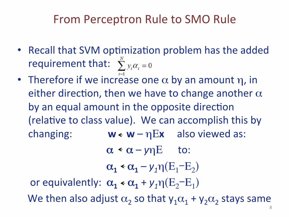
From  Perceptron  Rule  to  SMO  Rule  

•  Recall  that  SVM  opAmizaAon  problem  has  the  added  requirement  that:

•  Therefore  if  we  increase  one  α  by  an  amount  η,  in  either  direcAon,  then  we  have  to  change  another  α by  an  equal  amount  in  the  opposite  direcAon  (relaAve  to  class  value).    We  can  accomplish  this  by  changing:                            w        w  –  ηΕx          also  viewed  as:  

                                                                     α          α  –  yηΕ            to:                                                                        α1        α1  –  y1η(Ε1-Ε2)            or  equivalently:    α1        α1  +  y1η(Ε2-Ε1)          We  then  also  adjust  α2  so  that  y1α1  +  y2α2  stays  same  

 8  

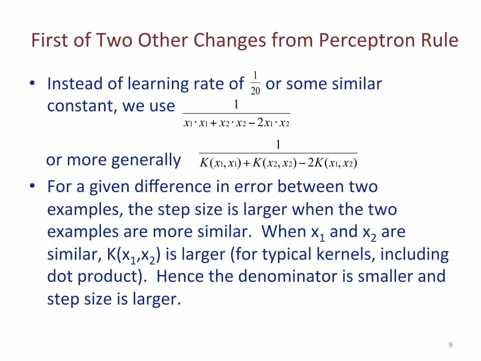
First  of  Two  Other  Changes  from  Perceptron  Rule  

•  Instead  of  learning  rate  of          or  some  similar  constant,  we  use

       or  more  generally  •  For  a  given  difference  in  error  between  two  examples,  the  step  size  is  larger  when  the  two  examples  are  more  similar.    When  x1  and  x2  are  similar,  K(x1,x2)  is  larger  (for  typical  kernels,  including  dot  product).    Hence  the  denominator  is  smaller  and  step  size  is  larger.

 

201

212211 21

xxxxxx ⋅−⋅+⋅

),(2),(),(1

212211 xxKxxKxxK −+

9  

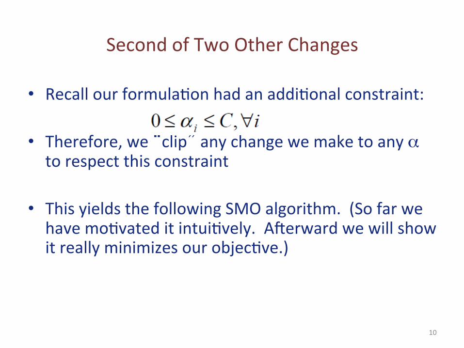
Second  of  Two  Other  Changes  

•  Recall  our  formulaAon  had  an  addiAonal  constraint:  

•  Therefore,  we  “clip”  any  change  we  make  to  any  α  to  respect  this  constraint  

•  This  yields  the  following  SMO  algorithm.    (So  far  we  have  moAvated  it  intuiAvely.    AWerward  we  will  show  it  really  minimizes  our  objecAve.)  

10  

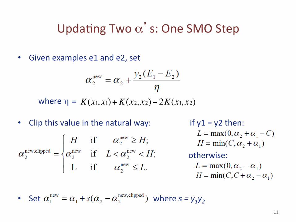
UpdaAng  Two  α’s:  One  SMO  Step  

•  Given  examples  e1  and  e2,  set                                                                                                                                                                                                                                                                                                                                                            where  η =  

•  Clip  this  value  in  the  natural  way:                                      if  y1  =  y2  then:  

•                                                                                                                                                             otherwise:  

•  Set                                                                                                              where  s  =  y1y2  11  

K(x1, x1)+K(x2, x2)− 2K(x1, x2)

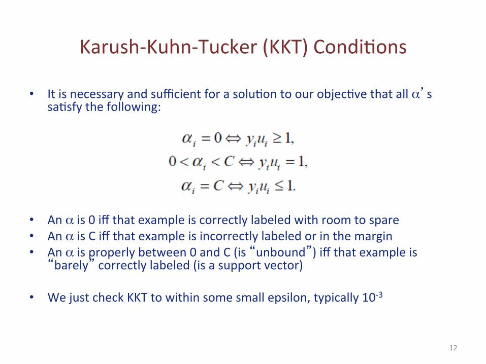
Karush-­‐Kuhn-­‐Tucker  (KKT)  CondiAons  

•  It  is  necessary  and  sufficient  for  a  soluAon  to  our  objecAve  that  all  α’s  saAsfy  the  following:  

 

•  An  α  is  0  iff  that  example  is  correctly  labeled  with  room  to  spare  •  An  α  is  C  iff  that  example  is  incorrectly  labeled  or  in  the  margin  •  An  α  is  properly  between  0  and  C  (is  “unbound”)  iff  that  example  is  “barely”  correctly  labeled  (is  a  support  vector)  

 •  We  just  check  KKT  to  within  some  small  epsilon,  typically  10-­‐3  

12  

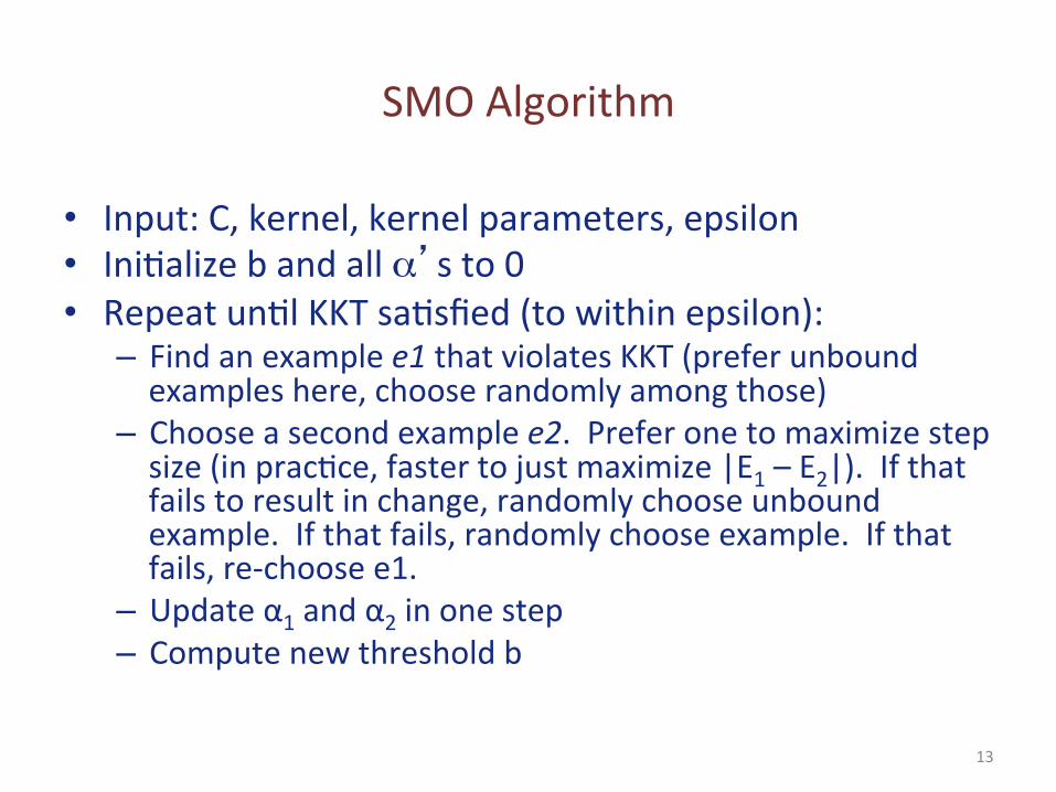
SMO  Algorithm  

•  Input:  C,  kernel,  kernel  parameters,  epsilon  •  IniAalize  b  and  all  α’s  to  0  •  Repeat  unAl  KKT  saAsfied  (to  within  epsilon):  

–  Find  an  example  e1  that  violates  KKT  (prefer  unbound  examples  here,  choose  randomly  among  those)  

–  Choose  a  second  example  e2.    Prefer  one  to  maximize  step  size  (in  pracAce,  faster  to  just  maximize  |E1  –  E2|).    If  that  fails  to  result  in  change,  randomly  choose  unbound  example.    If  that  fails,  randomly  choose  example.    If  that  fails,  re-­‐choose  e1.  

–  Update  α1  and  α2  in  one  step  –  Compute  new  threshold  b  

13  

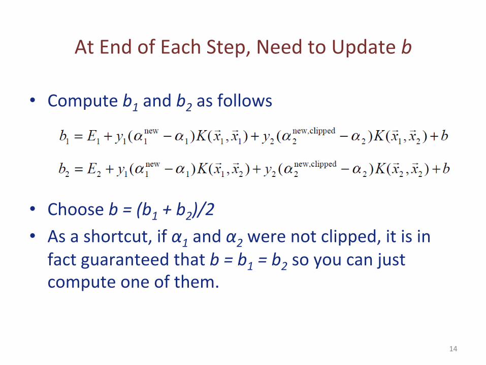
At  End  of  Each  Step,  Need  to  Update  b  

•  Compute  b1  and  b2  as  follows  

•  Choose  b  =  (b1  +  b2)/2  •  As  a  shortcut,  if  α1  and  α2  were  not  clipped,  it  is  in  fact  guaranteed  that  b  =  b1  =  b2  so  you  can  just  compute  one  of  them.  

14  

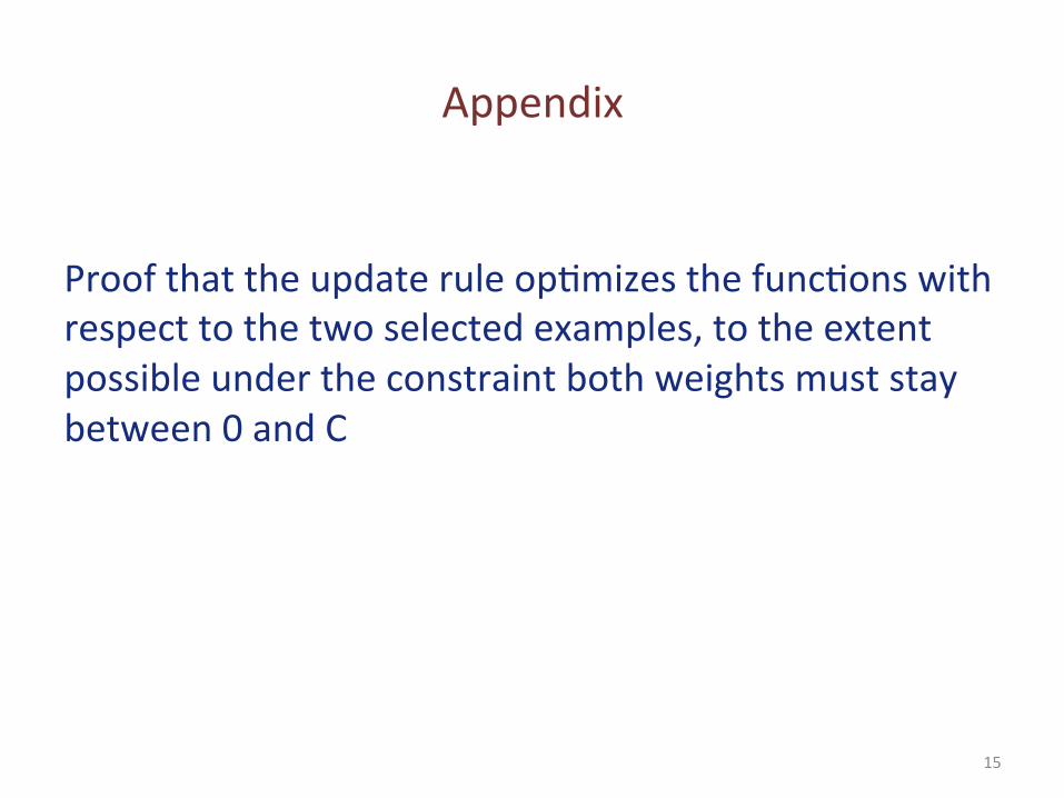
Appendix  

 Proof  that  the  update  rule  opAmizes  the  funcAons  with  respect  to  the  two  selected  examples,  to  the  extent  possible  under  the  constraint  both  weights  must  stay  between  0  and  C  

15  

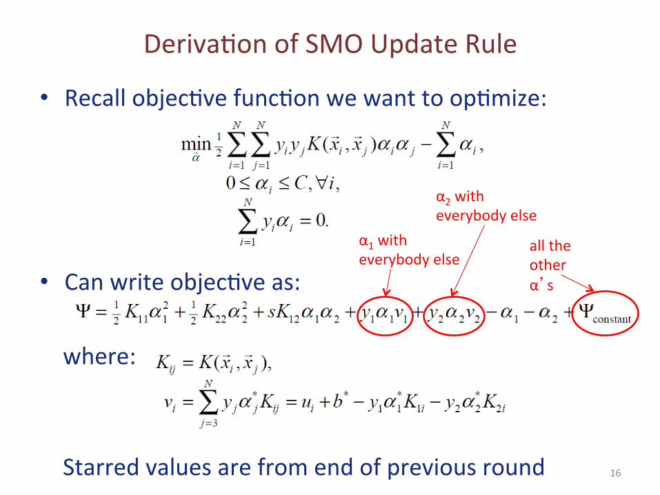
DerivaAon  of  SMO  Update  Rule  

•  Recall  objecAve  funcAon  we  want  to  opAmize:  

•  Can  write  objecAve  as:  

       where:                      Starred  values  are  from  end  of  previous  round      

α1  with  everybody  else  

α2  with  everybody  else  

all  the  other  α’s  

16  

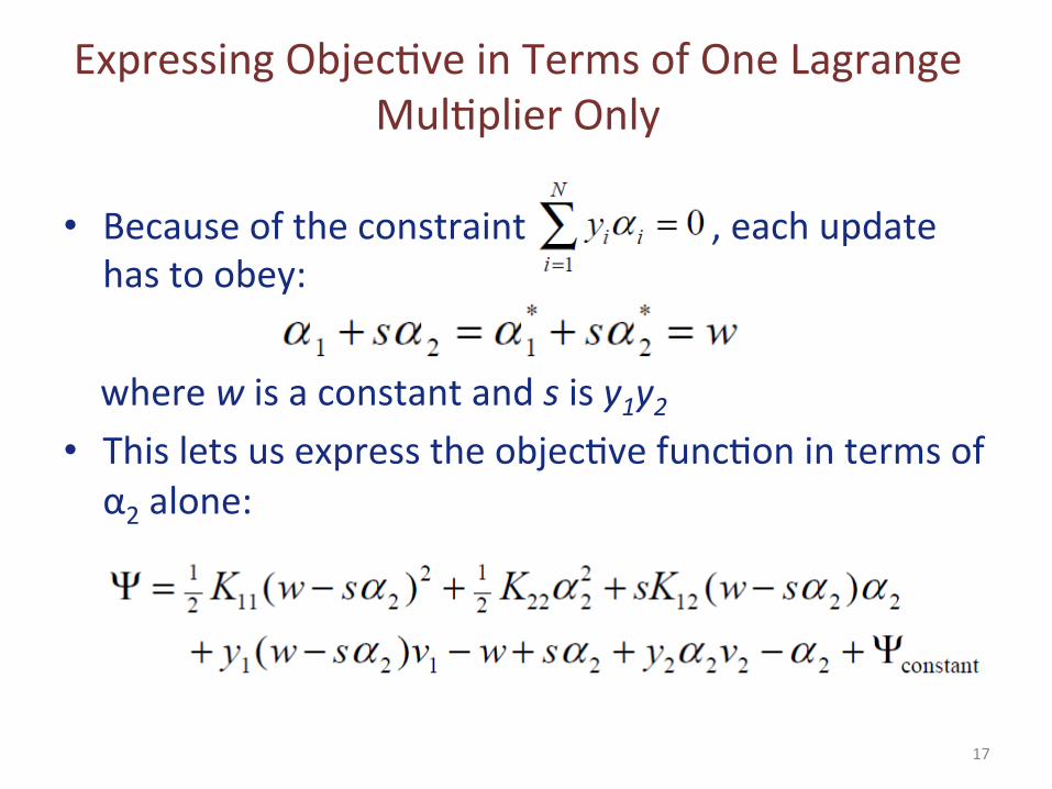
Expressing  ObjecAve  in  Terms  of  One  Lagrange  MulAplier  Only  

•  Because  of  the  constraint                                        ,  each  update  has  to  obey:    

                 where  w  is  a  constant  and  s  is  y1y2  •  This  lets  us  express  the  objecAve  funcAon  in  terms  of  α2  alone:  

17  

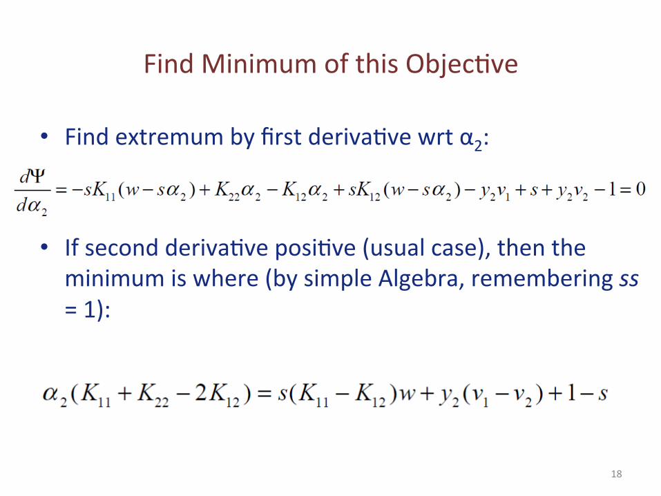
Find  Minimum  of  this  ObjecAve  

•  Find  extremum  by  first  derivaAve  wrt  α2:  

•  If  second  derivaAve  posiAve  (usual  case),  then  the  minimum  is  where  (by  simple  Algebra,  remembering  ss  =  1):  

18  

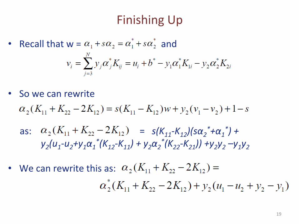
Finishing  Up  

•  Recall  that  w  =                                                                    and  

•  So  we  can  rewrite  

                   as:                                                                                            =      s(K11-­‐K12)(sα2

*+α1*)  +  

                           y2(u1-­‐u2+y1α1*(K12-­‐K11)  +  y2α2

*(K22-­‐K21))  +y2y2  –y1y2  

•  We  can  rewrite  this  as:      

19  

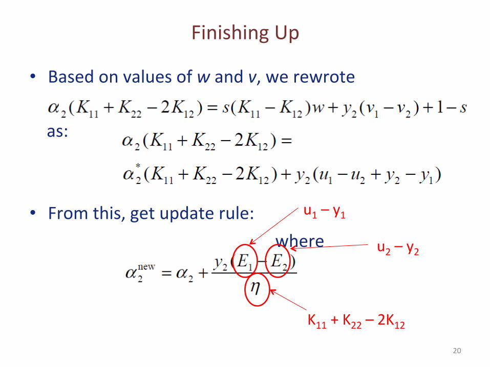
Finishing  Up  

•  Based  on  values  of  w  and  v,  we  rewrote  

       as:    

•  From  this,  get  update  rule:                                                                                                                    where  

u1  –  y1  

u2  –  y2  

K11  +  K22  –  2K12  20