Suzanne Paulson* & Nico Schulte** · IDENTIFYING URBAN DESIGNS AND TRAFFIC MANAGEMENT STRATEGIES FOR SOUTHERN CALIFORNIA THATREDUCE AIR POLLUTION EXPOSURE. Suzanne Paulson* & Nico

IDENTIFYING URBAN DESIGNS AND TRAFFICMANAGEMENT STRATEGIES FOR SOUTHERN CALIFORNIA

THAT REDUCE AIR POLLUTION EXPOSURE

Suzanne Paulson* & Nico Schulte**Wonsik Choi,* J.R. DeShazo,* Dilhara Ranasinghe,*

Akula Venkatram,** Lisa Wong,* Owen Hearey,* Karen Bunavage,* Rodrigo Siguel,* Arthur Winer,*

Mario Gerla,* Kathleen Kozawa,*** Steve Mara,*** Si Tan**

*UCLA Departments of Atmospheric and Oceanic Sciences, Institute of Environment and Sustainability,

Public Policy, Luskin Center for Innovation, Computer Science & Environmental Health Sciences

**UCR Department of Mechanical Engineering

***CARB

1

Objectives• Develop guidelines for TOD planners to reduce pedestrian

exposure to air pollution in urban built environments through field measurements, analysis and statistical modeling.

• Develop a dispersion model that can be used to provide TOD planners quantitative links among the variables that control dispersion in complex urban environments.

2

Introduction: Air Pollution Near Roadways & Their Health Impacts

3

Air pollutants from traffic sources

4

• Oxides of Nitrogen• Volatile Organic Compounds, including some air toxics• Ultrafine Particles (UFP)• Brake dust• UFP and the gasses undergo similar dispersion in the

atmosphere.

Pollutant Concentrations Near Roadways Vary A LOT• Fleet emissions

• Traffic density, fleet composition, driving conditions• Atmospheric Dispersion

• Wind speed and direction, atmospheric stability, vehicle wakes, topography

• Built Environment• Roadway geometry, buildings, soundwalls, other

nearby roadways & vegetation• Observed roadway pollutant spatial distributions also

depend on the relationship between the peak and background concentrations.

5

Fine Coarse

Very fine dust from mechanical processes

Mostly formed in the atmosphere

Directly emitted or formed in the atmosphere

Very Small Particles: lots of spatial heterogeneity

Ultrafine particles are mostly from vehicular emissions. They disappear In around a half an hour: rather than magically going away, they collide and stick to fine particles. As a result, they are highly elevated around roadways compared to everywhere else.

Plot Source: Wilson et al. (1977)

Ultrafine

“Par

ticle

Mas

s”

Particle Diameter (microns)

6

Tropospheric Aerosols are Complex Mixtures

Numbers range from 103 to 107 cm-1 in urban areas

Soot Agglomerate

Liquid Droplet

Included Accumulation Mode Particles Diesel

Exhaust

Diesel Particle Close-up

PM2.5 particle

7

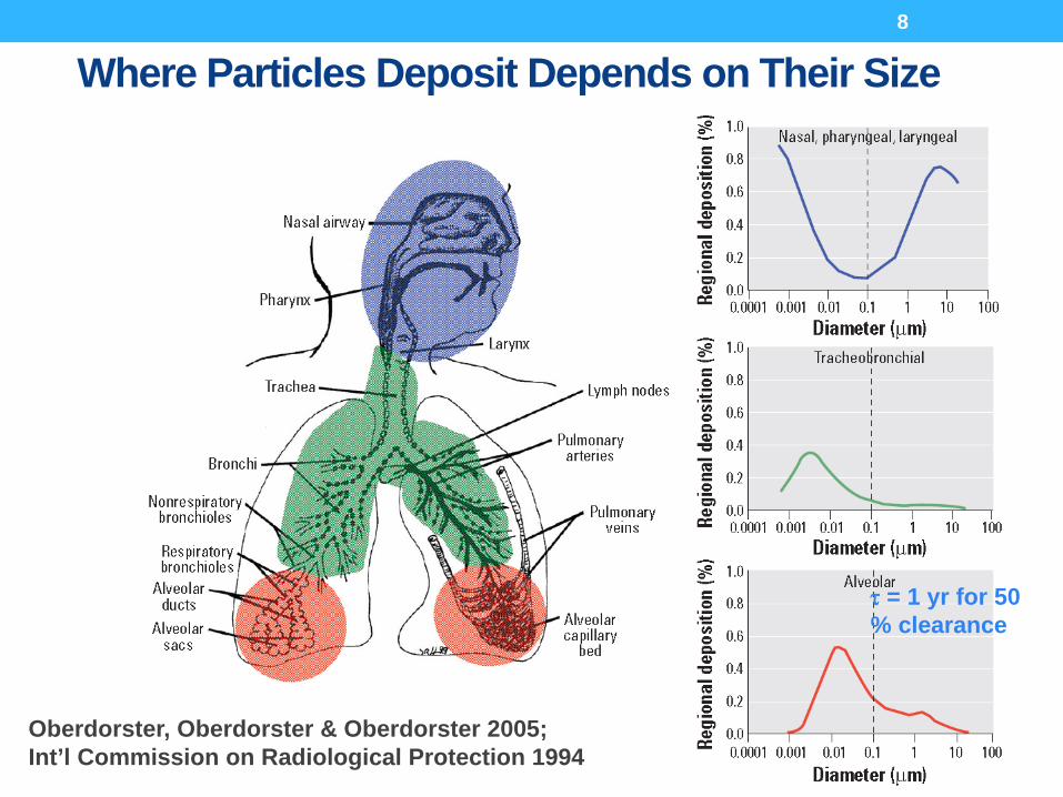
Oberdorster, Oberdorster & Oberdorster 2005; Int’l Commission on Radiological Protection 1994

τ = 1 yr for 50% clearance

Where Particles Deposit Depends on Their Size8

1µm0.1µm(and smaller)

E.R. Weibel, University of Bern

TRANSLOCATION FROM AIR TO BLOOD

Courtesy of Peter Gehr, U. Bern

9

Multiple Pathways to Increased Morbidity in Children are Associated with Proximity to Traffic

Prenatal Impacts Los Angles - women living near high heavy duty traffic areas were

at increased risk of premature delivery and low birth weight babies (Ritz and Co-workers, UCLA)

Asthma Prevalence Southern California - prevalence of asthma among children was

associated with several indicators of exposure to traffic including proximity of the home to a freeway

Respiratory Symptoms East Bay (San Francisco area) - children attending schools near

freeways had more respiratory symptoms

10

Multiple Pathways to Increased Morbidity & Mortality in Adults are Associated with Proximity to Traffic

• Acute respiratory diseases; • acute asthma, chronic obstructive pulmonary disease, pneumonia,

lung cancer

• Cardiovascular disease; • Heart attacks and stroke

• Many other diseases • Air pollution degrades overall health, beginning prior to birth. This

results in higher incidences of many diseases and conditions.

11

What makes UFPs distinct from other pollutants includes:

Source strengtha wide variability in particle number emission factors which depend on fuel and engine types, maintenance and age of vehicles, driving conditions, etc

[Morawska et al., 2008]

Dynamic nature

short lifetime (~ hours) and on-going transformation of their physical and chemical properties including number and size distributions which decreases with increasing particle size

[Birmili et al., 2013; Choi et al., 2016a]

Atmos. dispersion

governed by wind speed/direction, atmospheric stability, and “breathability” of cities which depends on the urban morphology (built-environment)

[Buccolieri et al., 2010; Choi et al., 2016b]

Substantial temporal and spatial variability of UFPs distributions both in number and sizes

Spatial heterogeneity of UFPs (and inventory) remains a key challengefor the assessment of their impacts on human health and climate

12

APPROACHESStationary measurementsMobile measurements

13

Field Measurement Areas

Down Town Los Angeles

Temple City

Beverly Hills

Riverside

14

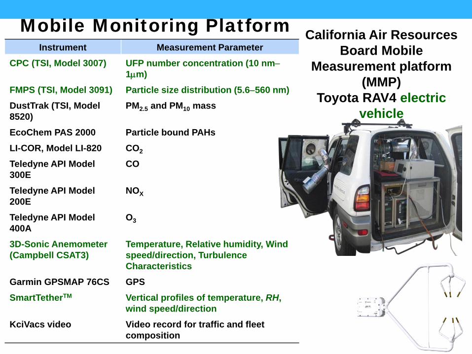
Instrument Measurement ParameterCPC (TSI, Model 3007) UFP number concentration (10 nm−

1µm)FMPS (TSI, Model 3091) Particle size distribution (5.6−560 nm)DustTrak (TSI, Model 8520)

PM2.5 and PM10 mass

EcoChem PAS 2000 Particle bound PAHsLI-COR, Model LI-820 CO2

Teledyne API Model 300E

CO

Teledyne API Model 200E

NOX

Teledyne API Model 400A

O3

3D-Sonic Anemometer(Campbell CSAT3)

Temperature, Relative humidity, Wind speed/direction, Turbulence Characteristics

Garmin GPSMAP 76CS GPSSmartTetherTM Vertical profiles of temperature, RH,

wind speed/directionKciVacs video Video record for traffic and fleet

composition

California Air Resources Board Mobile

Measurement platform(MMP)

Toyota RAV4 electric vehicle

Mobile Monitoring Platform

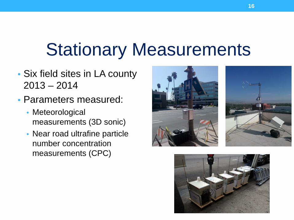
• Six field sites in LA county 2013 – 2014

• Parameters measured:• Meteorological

measurements (3D sonic)• Near road ultrafine particle

number concentration measurements (CPC)

16

Stationary Measurements

“Roadmap”• Introduction• The impact of the dimensions on pollution in street

canyons (N. Schulte)• Results of high spatial resolution (~5 m) mobile &

stationary measurements made in 5 neighborhoods in Los Angeles• High fidelity processing of mobile measurements• A microdynamics model for predicting concentrations along the

street• The neighborhood view: The impact of the design of the built

environment on the scale of several large city blocks• Benefits of locating the bus stops a bit further from the

intersections• Summary for Planners

17

RESULTS

18

Street Canyons

Nico Schulte, Si Tan and Akula Venkatram (2015) The ratio of effective building height to street width governs dispersion of local vehicle

emissions. Atmos. Environ. 11:54–63.

19

20

0

1

2

3

0 10 20

Mag

nific

atio

n

Building Height [m]

Objective and Model ApplicationTo develop models that account for building effects in linking vehicle emissions to near road pollutant concentrations.

Models validated with field data can be used to conduct numerical experiments that would be impossible in the real world.

Evaluate impact of designs for transit oriented development on near-road concentrations of traffic emissions

Evaluate mitigation methods including traffic management, limiting building height, creating open space, pedestrian zones

21

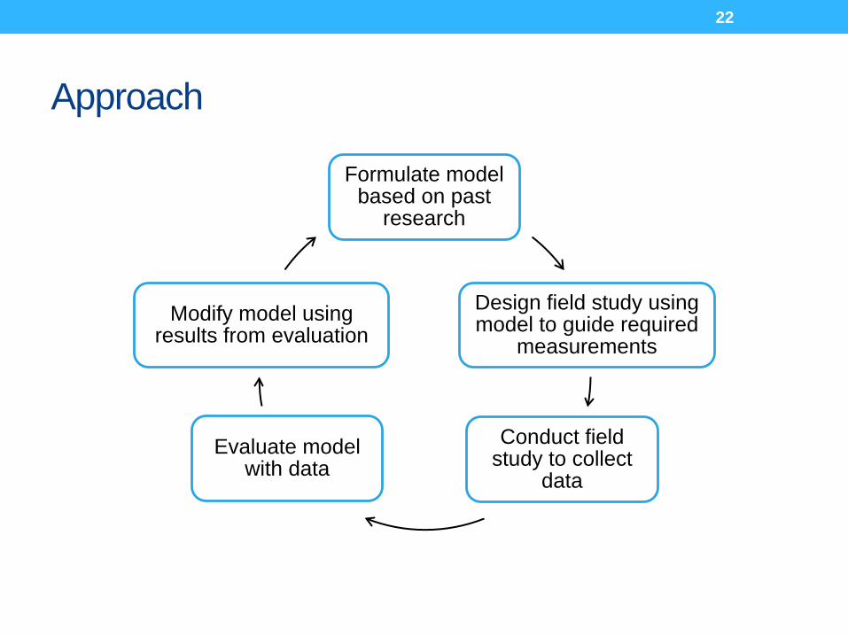
Approach

22

Formulate model based on past

research

Design field study using model to guide required

measurements

Conduct field study to collect

dataEvaluate model

with data

Modify model using results from evaluation

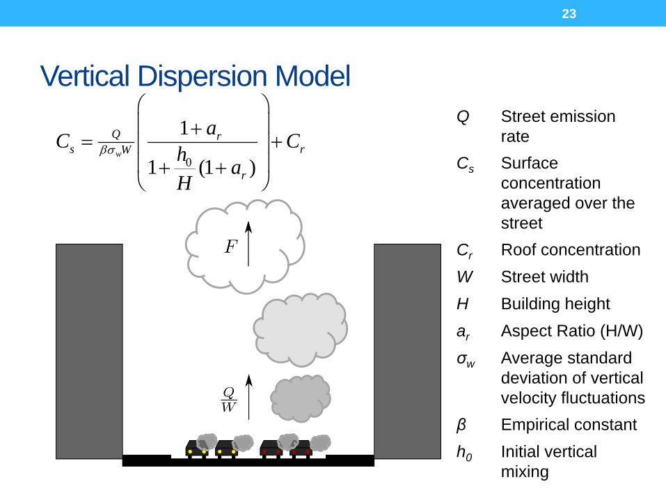
Vertical Dispersion Model

23

Q Street emission rate

Cs Surface concentration averaged over the street

Cr Roof concentrationW Street widthH Building heightar Aspect Ratio (H/W)σw Average standard

deviation of vertical velocity fluctuations

β Empirical constanth0 Initial vertical

mixing

0

1

1 (1 )w

Q rs rW

r

aC Ch aH

βσ

+

= + + +

Area Weighted Building HeightL Length of streethi Height of building ibi Length of building i along street

24

1i iL

iH h b= ∑

Left: Google earth view of 8th St LA field site. Right: Building heights along 8th St

Evaluation with LA county data

• Six field sites in LA county 2013 –2014

• Near road ultrafine particle number concentration measurements

25

Left: Scatter plot (normalized by emission rate)Right: q-q plot. 30 minute average UFP concentrations

Evaluation with Riverside data

• August/September 2015 Riverside Market Street

• Carbon monoxide and UFP measurements

26

Top: Scatter plot, Bottom: q-q plot. 2 hour average CO concentrations

Evaluation with Riverside data

27

2 hour average CO concentrations normalized by traffic emission rate

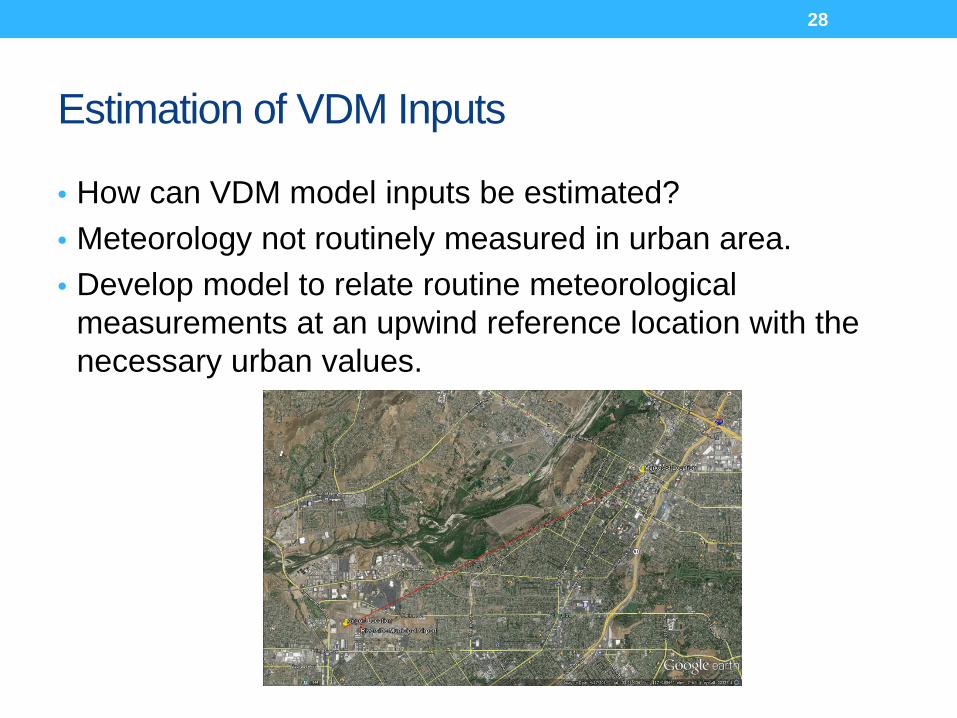
Estimation of VDM Inputs

• How can VDM model inputs be estimated?• Meteorology not routinely measured in urban area.• Develop model to relate routine meteorological

measurements at an upwind reference location with the necessary urban values.

28

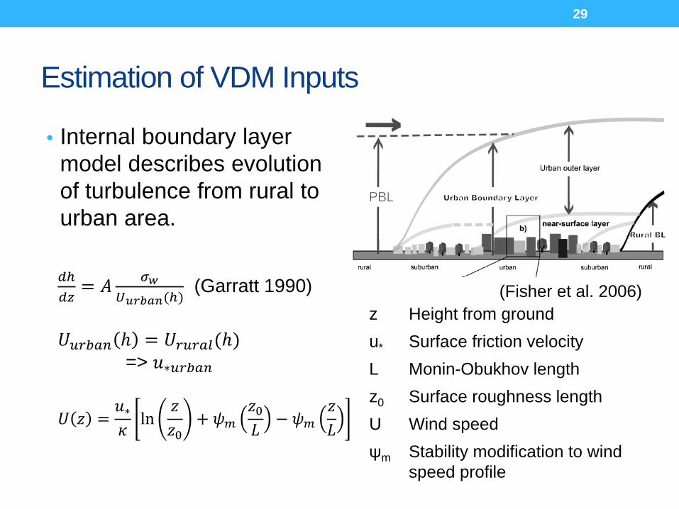
Estimation of VDM Inputs

z Height from groundu* Surface friction velocityL Monin-Obukhov lengthz0 Surface roughness lengthU Wind speedψm Stability modification to wind

speed profile

• Internal boundary layer model describes evolution of turbulence from rural to urban area.

29

(Fisher et al. 2006)𝑑𝑑𝑑𝑑𝑑𝑑𝑑

= 𝐴𝐴 𝜎𝜎𝑤𝑤𝑈𝑈𝑢𝑢𝑢𝑢𝑢𝑢𝑢𝑢𝑢𝑢(𝑑)

(Garratt 1990)

𝑈𝑈𝑢𝑢𝑢𝑢𝑢𝑢𝑢𝑢𝑢𝑢 ℎ = 𝑈𝑈𝑢𝑢𝑢𝑢𝑢𝑢𝑢𝑢𝑟𝑟(ℎ)=> 𝑢𝑢∗𝑢𝑢𝑢𝑢𝑢𝑢𝑢𝑢𝑢𝑢

𝑈𝑈 𝑧𝑧 =𝑢𝑢∗𝜅𝜅

ln𝑧𝑧𝑧𝑧0

+ 𝜓𝜓𝑚𝑚𝑧𝑧0𝐿𝐿

− 𝜓𝜓𝑚𝑚𝑧𝑧𝐿𝐿

Implications for Policy

• Ratio of area weighted building height to street width, the effective aspect ratio, governs near-road concentrations.

• VDM suggests that the effective aspect ratio of streets with high local vehicle traffic should be limited to reduce exposure to elevated concentrations of traffic emissions.

30

Project Outcome – UCR VDM Tool• Combine VDM + AERMOD for

practical application by planners

31

Develop project level emission estimates

Use AERMOD to compute Cr (with standard urban

options)

Compute building morphological parameters

(from digital elevation model)

Use VDM tool to compute surface concentration CsVDM GUI interface

Model is available to download at https://www.arb.ca.gov/research/single-project.php?row_id=65135

https://www.arb.ca.gov/research/single-project.php?row_id=65135

Processing Mobile Data

Ranasinghe, D., W.S. Choi, A.M. Winer and S.E. Paulson (2016) Developing High Spatial Resolution Concentration Maps Using Mobile

Air Quality Measurements. Aerosol and Air Qual. Res. 16 (8), 1841-1853.

Broadway and & 7th, Downtown LA33

Mobile Data Challenges• Mobile data gives spatially heterogeneous measurements; sometimes you get 30 measurements in one place; sometimes one every 20 m.

• Simple averaging of mobile data (after correction for the wandering GPS signal) ends up looking like a trail of confetti after a parade route.

• How many runs do you need?

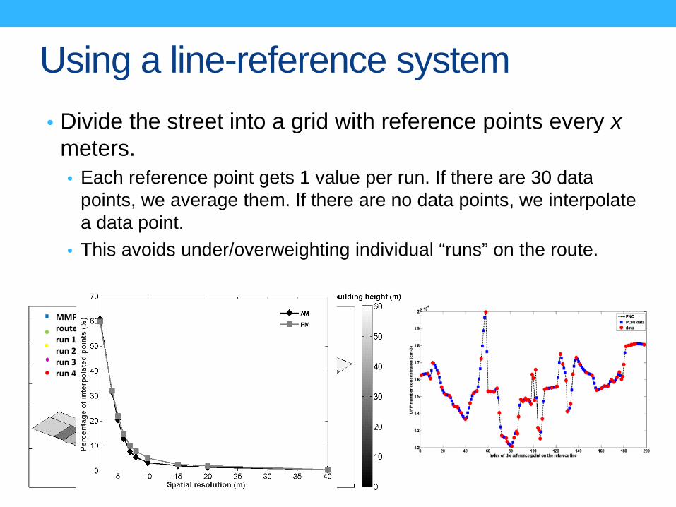
Using a line-reference system• Divide the street into a grid with reference points every x

meters. • Each reference point gets 1 value per run. If there are 30 data

points, we average them. If there are no data points, we interpolate a data point.

• This avoids under/overweighting individual “runs” on the route.

MMProuterun 1run 2run 3run 4

5 meter Spatial Resolution Map for Downtown Los Angeles

36

Need ~20 repeats under similar met conditions to get a reasonable average

Ranasinghe et al. AAQR (2016)

Morning

With high emitter spikes High emitter spikes removed

Afternoon

Some features appear consistently

Modeling the Determinants of Highly-localized UFP

Concentrations

J.R. DeShazo, Suzanne Paulson, Lisa Wu, Owen Hearey, and others

39

Data uses in Model• April-July 2008 • 2nd St. to Jefferson Blvd.• ~3 miles long • 12 MMP runs • ~7000 observations

Broadway Transect in Downtown Los Angeles

40

Why take this approach?1. How much of the observed variation UFP can be

attributed to each explanatory variable? How accurately can we measure these relationships?

2. How much of the observed UFP can be explained by these localized factors? Which local factors we leaving out? How much of the observed variation cannot be explained by accounting for local factors?

3. Estimated model can be used to prediction/simulate concentrations at any location for any configuration and level of factors.

41

Figure 2: Intersection Diagram with MMP42

Modeling the effects of highly-localized factors UFP = f(emission sources,

+ atmospheric conditions, + built environment, + position of the MMP, + constant (background concentration)

Regression model will seek to explain the concentration of UPF measure as function of a these explanatory variables.

43

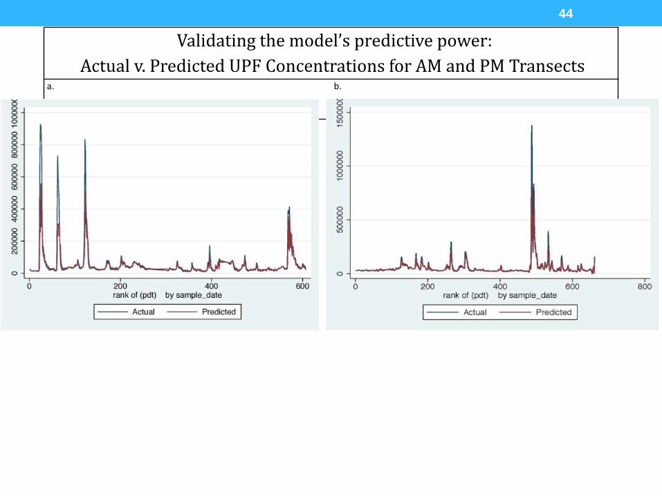
Validating the model’s predictive power: Actual v. Predicted UPF Concentrations for AM and PM Transects

a. b.

44

Three types of findings• 1. Cumulative impacts of factors on street level UFP,

• 2. Dynamic UFP patterns associated with common traffic events,

• 3. Predicted free-flow versus stop start UFP spatial and temporal dynamics

45

1. Cumulative impacts of factors on street level UFP

• How much does each of these factors explain that variation observed in UFP?

• We estimate the cumulative effect of a given variable on UFP by placing all of the other parameters at their mean values. We then estimate the predicted concentration of UFP when the variable of interest is set to zero, and compared that with predicted UFP concentration when the variable of interest is set to its mean level.

• Next slide highlights the top five factors

46

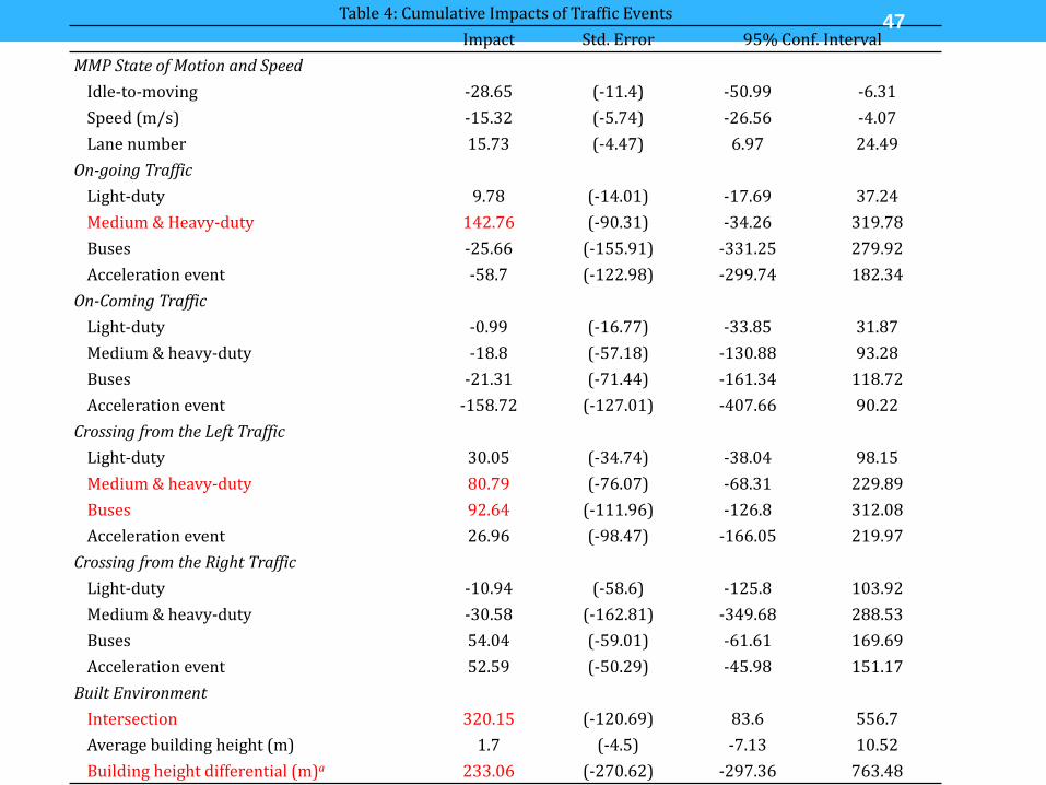
Table 4: Cumulative Impacts of Traffic EventsImpact Std. Error 95% Conf. Interval

MMP State of Motion and SpeedIdle-to-moving -28.65 (-11.4) -50.99 -6.31Speed (m/s) -15.32 (-5.74) -26.56 -4.07Lane number 15.73 (-4.47) 6.97 24.49

On-going TrafficLight-duty 9.78 (-14.01) -17.69 37.24Medium & Heavy-duty 142.76 (-90.31) -34.26 319.78Buses -25.66 (-155.91) -331.25 279.92Acceleration event -58.7 (-122.98) -299.74 182.34

On-Coming TrafficLight-duty -0.99 (-16.77) -33.85 31.87Medium & heavy-duty -18.8 (-57.18) -130.88 93.28Buses -21.31 (-71.44) -161.34 118.72Acceleration event -158.72 (-127.01) -407.66 90.22

Crossing from the Left TrafficLight-duty 30.05 (-34.74) -38.04 98.15Medium & heavy-duty 80.79 (-76.07) -68.31 229.89Buses 92.64 (-111.96) -126.8 312.08Acceleration event 26.96 (-98.47) -166.05 219.97

Crossing from the Right TrafficLight-duty -10.94 (-58.6) -125.8 103.92Medium & heavy-duty -30.58 (-162.81) -349.68 288.53Buses 54.04 (-59.01) -61.61 169.69Acceleration event 52.59 (-50.29) -45.98 151.17

Built EnvironmentIntersection 320.15 (-120.69) 83.6 556.7Average building height (m) 1.7 (-4.5) -7.13 10.52Building height differential (m)a 233.06 (-270.62) -297.36 763.48

47

2. Dynamic UFP patterns associated with common traffic events • Model Characterizes Dynamic Traffic Events:

• UFP patterns associated with • Traffic crossing at an intersection in front of the MMP as it is

stopped at a light,• Oncoming heavy duty vehicles in traffic while the MMP travels• Ongoing and oncoming accelerations events from the stopped

position while the MMP accelerates from a stopped position traveling with ongoing traffic.

48

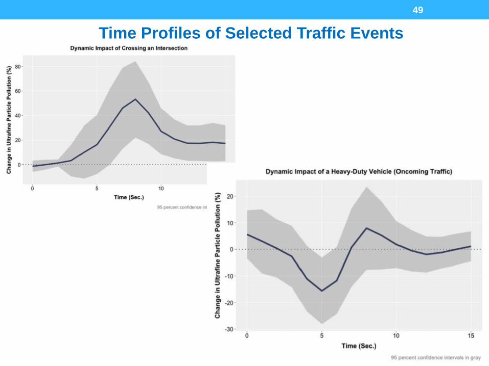
Time Profiles of Selected Traffic Events49

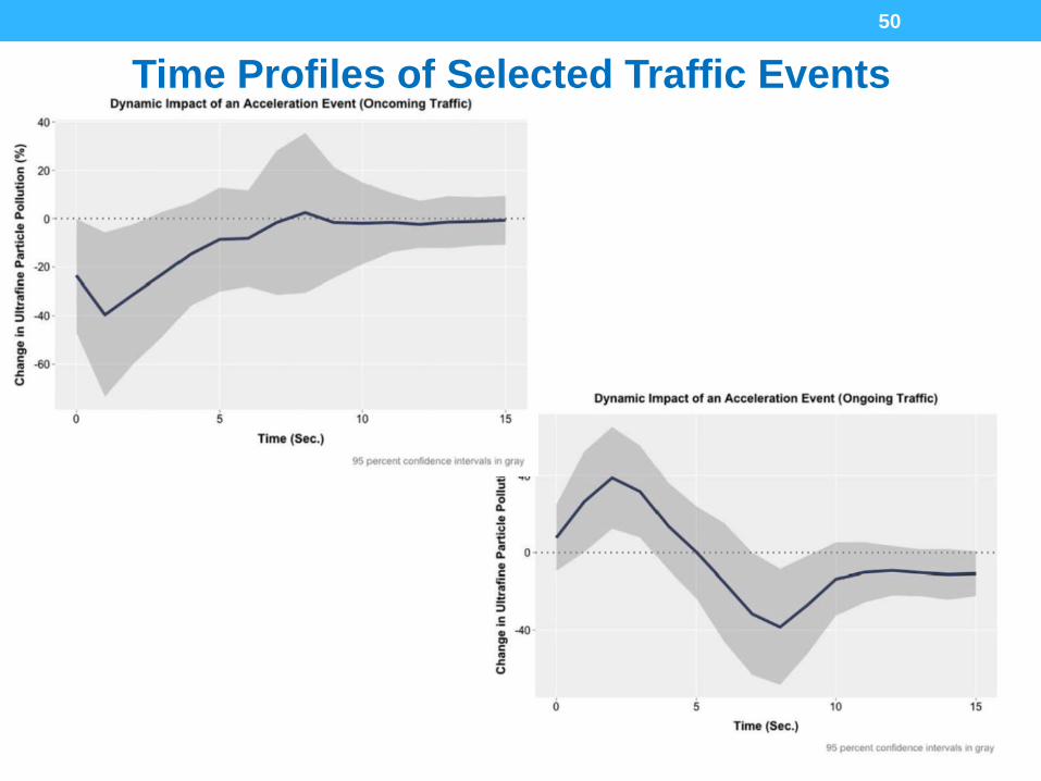
Time Profiles of Selected Traffic Events50

We do two planning/policy simulations

A. What happens to free-flow vs stop/start?

B. What happens when there are more or less light duty vehicles, heavy duty, etc

3. Predicted free-flow versus stop start UFP spatial and temporal dynamics

51

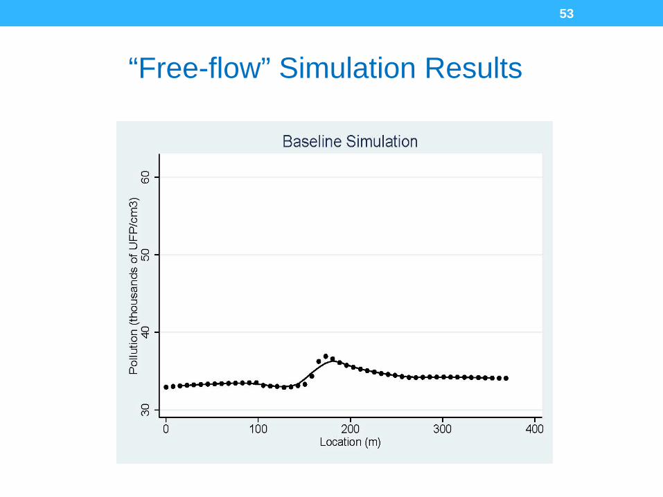
• MMP cruises for 225m/30 sec. at constant speed (7.5 m/s) across an intersection

• All neighboring buildings are 15m high; the intersection is 12m across (from 103 to 115)

• Wind and location fixed effects are set to long-run averages

• No acceleration instances occur, and no cross-traffic is encountered

• Ongoing and oncoming traffic are set to long-run averages

“Free-flow” simulation

52

53

“Free-flow” Simulation Results

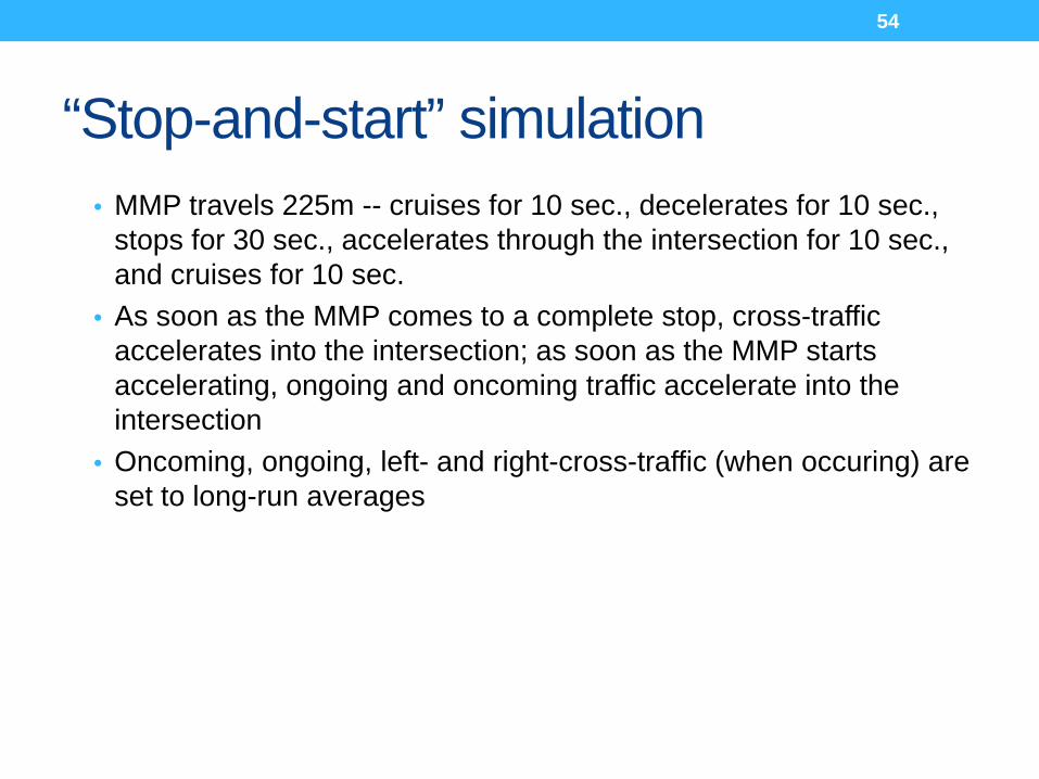
• MMP travels 225m -- cruises for 10 sec., decelerates for 10 sec., stops for 30 sec., accelerates through the intersection for 10 sec., and cruises for 10 sec.

• As soon as the MMP comes to a complete stop, cross-traffic accelerates into the intersection; as soon as the MMP starts accelerating, ongoing and oncoming traffic accelerate into the intersection

• Oncoming, ongoing, left- and right-cross-traffic (when occuring) are set to long-run averages

“Stop-and-start” simulation

54

55

“Stop-Start” Simulation Results

56

Adding 75% more light duty to Free-flow” Simulation Results

Choi, W., D. Ranasinghe, K. Bunavage, J.R. DeShazo, L. Wu, R. Seguel, A.M. Winer, and S.E. Paulson (2016)

The effects of the built environment, traffic patterns, and micrometeorology on street level ultrafine particle concentrations

at a block scale: Results from multiple urban sites. Sci. Tot. Environ. 15;553:474-85. doi: 10.1016/j.scitotenv.2016.02.083.

What is the effect of the built environment at the

block/neighborhood scale on pollutant concentrations at the

street?

57

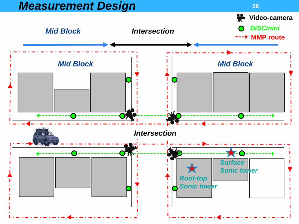
Roof-top Sonic tower

SurfaceSonic tower

Mid Block Mid Block

Mid Block Intersection

Intersection

DiSCminiMMP route

Video-cameraMeasurement Design 58

-118.26 -118.255 -118.25 -118.245

34.038

34.04

34.042

34.044

34.046

34.048

34.05

34.052

Longitude ( o )

Latit

ude

( o )

0

100

200

300

400

500

Site 1: Street Canyon

Broadway & 7th Site (Street view: heading South)

Building height(Ft.)

59

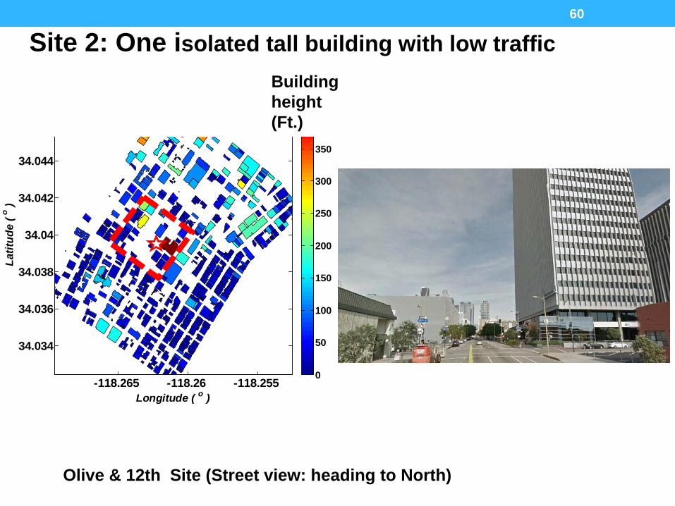
-118.265 -118.26 -118.255

34.034

34.036

34.038

34.04

34.042

34.044

Longitude ( o )

Latit

ude

( o )

0

50

100

150

200

250

300

350

Olive & 12th Site (Street view: heading to North)

Site 2: One isolated tall building with low trafficBuilding height (Ft.)

60

-118.296 -118.292 -118.28834.056

34.057

34.058

34.059

34.06

34.061

34.062

34.063

34.064

Longitude ( o )

Latit

ude

( o )

50

100

150

200

250

300

350

Vermont & 7th Site (Street view: heading to West)

Site 3: One isolated tall building with high traffic


61

-118.284 -118.282 -118.28 -118.278 -118.27634.056

34.058

34.06

34.062

34.064

Longitude ( o )

Latit

ude

( o )

0

50

100

150

200

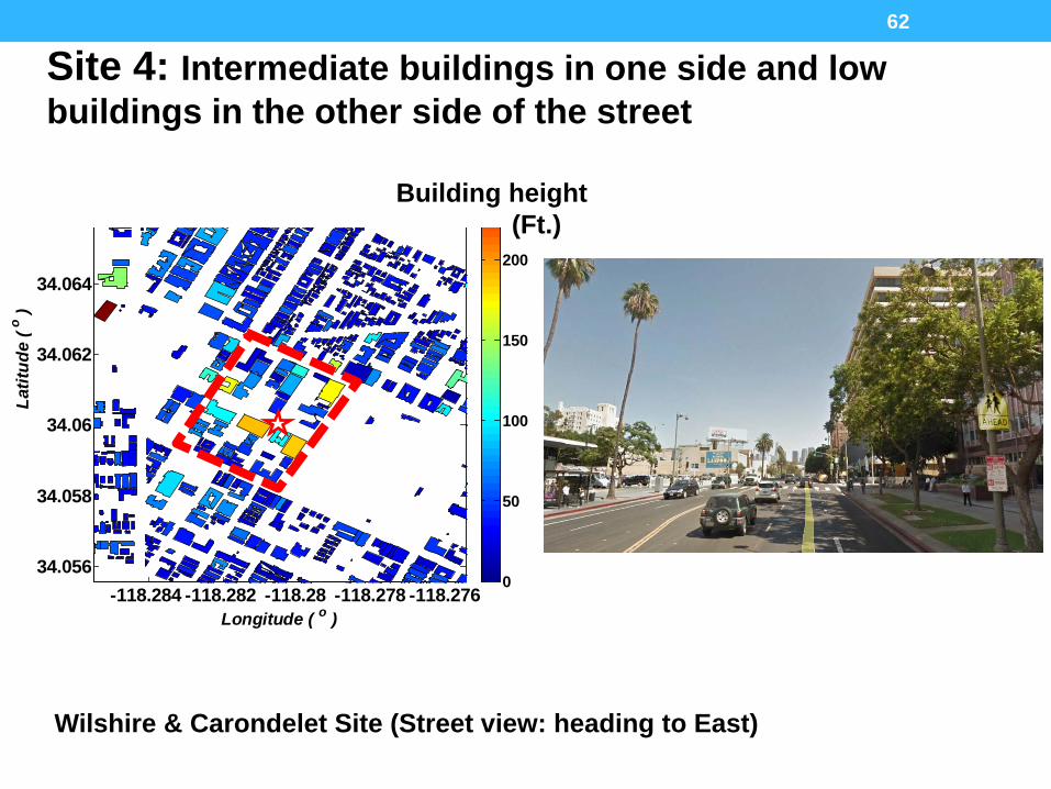
Wilshire & Carondelet Site (Street view: heading to East)

Site 4: Intermediate buildings in one side and low buildings in the other side of the street


62

-118.0662 -118.0622 -118.058234.1021

34.1041

34.1061

34.1081

34.1101

Longitude ( o )

Latit

ude

( o )

10

15

20

25

30

35

Temple City & Las Tunas Site (Street view: heading to North)

Site 5: All single story buildings


63

Built environment quantitative descriptors Broadway

& 7th

(Site1)

Olive St. &

12th St. (Site2)

Vermont &

7th St. (Site3)

Wilshire &

Carondelet (Site4)

Temple City &

Las Tunas (Site5)

# of buildings 59 34 90 44 143

Max. building height (m) 58 129 80 57 8

Mean building height, Hbldg (m)

34 21 11 18 5

Bldg area weighted height, Harea (m)

40 42 25 24 6

Bldg. homogeneity, Harea/Hbldg (dimensionless) (1=perfectly homogeneous)

1.16 2.01 2.21 1.39 1.09

Mean building ground area (m2)

1,030 1,395 585 992 225

Street width (m) 26 (BW) / 22 (7th)

28 (Olive) / 17 (12th)

30 (Ver) / 25 (7th)

17 (Car) / 37 (Wil)

24 (TC) / 30 (LT)

Simple Aspect ratio (Harea/Wstreet)

1.7 1.9 0.9 0.9 0.2

Block length (m) 190 (BW) / 100 (7th)

180 (Olive)/ 95 (12th)

190 (Ver) / 95 (7th)

160 (Car) / 75 (Wil)

175 (TC) / 115 (LT)

Ratio occupied by bldg. 0.72 0.42 0.33 0.46 0.30

64

(a) Morning (b) Afternoon

Higher traffic generally higher UFP. In the morning howeverthere are deviations esp. for the two sites with extreme built-environments: the street canyon (Site1) and the low, flat bldg. canopy (Site 5).

65

0 10 20 30 40 50 60 7010

15

20

25

30

35

40

45

[UFP

] (

×10

3pa

rtic

les

⋅cm

-3)

Traffic flow rate (vehicles⋅min-1)10 20 30 40 50 60 70

10

15

20

25

30

35

40

45

[UFP

] (

× 103

part

icle

s⋅c

m-3

)

Traffic flow rate (vehicles⋅min-1)

Site 1Site 2Site 3Site 4Site 5

(a) (b)

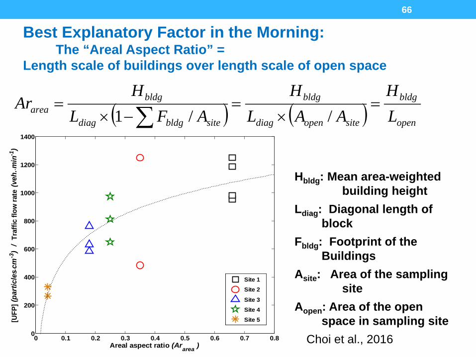
Best Explanatory Factor in the Morning: The “Areal Aspect Ratio” =

Length scale of buildings over length scale of open space

( ) ( ) open

bldg

siteopendiag

bldg

sitebldgdiag

bldgarea L

HAAL

HAFL

HAr =

×=

−×=

∑ //1

Hbldg: Mean area-weighted building height

Ldiag: Diagonal length of block

Fbldg: Footprint of the Buildings

Asite: Area of the sampling site

Aopen: Area of the open space in sampling site

0 0.1 0.2 0.3 0.4 0.5 0.6 0.7 0.80

200

400

600

800

1000

1200

1400

Areal aspect ratio (Ararea )

[UFP

] (pa

rtic

les ⋅

cm-3

) /

Traf

fic fl

ow ra

te (v

eh. ⋅m

in-1

)

Site 1Site 2Site 3Site 4Site 5

Choi et al., 2016

66

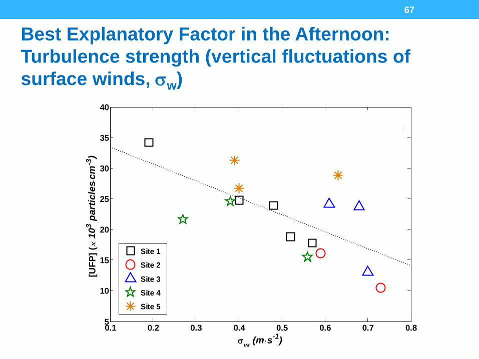
Best Explanatory Factor in the Afternoon: Turbulence strength (vertical fluctuations of surface winds, σw)

1800

n-1)

0.1 0.2 0.3 0.4 0.5 0.6 0.7 0.85

10

15

20

25

30

35

40

σw (m⋅s-1)

[UFP

] (×

103 p

artic

les ⋅

cm-3

)

Site 1Site 2

Site 3Site 4Site 5

(a)

67

Best Explanatory Factor in the Afternoon: Turbulence strength (vertical fluctuations of surface winds, σw)

Appears to be from non-local emissions

0.1 0.2 0.3 0.4 0.5 0.6 0.7 0.80

200

400

600

800

1000

1200

1400

1600

1800

σw ( m⋅s-1)

[UFP

] (pa

rtic

les ⋅

cm-3

) /

Traf

fic fl

ow ra

te (

veh.

⋅min

-1)

Fitting curvesSite 1Site 2Site 3Site 4Site 5

σw (m s )

(b)

68

The effects of building heterogeneity on turbulence in the afternoon:

Higher building heterogeneity appears to enhance surface turbulence, under conditions with moderate winds and an unstable atmosphere

1 1.2 1.4 1.6 1.8 2 2.20

0.5

1

1.5

2

2.5

Building heterogeneity (Harea / Hbldg)

Turb

ulen

ce k

inet

ic e

nerg

y (T

KE)

, m

2 ⋅s-2

1 1.2 1.4 1.6 1.8 2 2.20.1

0.2

0.3

0.4

0.5

0.6

0.7

0.8

Building heterogeneity (Harea / Hbldg)

σw

(m

⋅ s-1

)

Site 1

Site 2

Site 3

Site 4

Site 5

(a) (b)

σ w(m

∙s-1

)

Turb

ulen

ce k

inet

ic e

nerg

y (m

2 ∙s-1

)

69

Decay of pollutants around the intersections: the best

place for the bus stop?Choi, W.S., D. Ranasinghe, J.R. DeShazo, J.J. Kim and S.E.

Paulson (2017) Cross-Intersection Profiles of Ultrafine Particles in Different Built Environments: Implications for Pedestrian Exposure and Bus Transit Stops. Submitted.

70

How Far Should the Bus Stop be from the Intersection?

71

Near SideFar Side

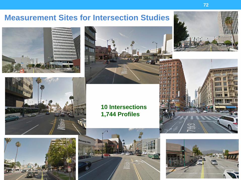
10 Intersections 1,744 Profiles

Measurement Sites for Intersection Studies72

Variety of Intersections; 1,744 Profiles TotalWilshire in

Beverly Hills

(5 inter-sections)

Broadway & 7th

Downtown Los

Angeles

Olive & 12th

Downtown Los

Angeles

Vermont & 7th

Wilshire & Carondelet

Temple City & Las

Tunas

Street width

30 - 38 m 22 & 26 m 17 & 28 m 25 & 30 m 17 & 37 m 24 & 30 m

Traffic flow rate (A.M.)

24 12 & 15 21 & 4 39 & 10 31 & 31 25 & 28

Traffic flow rate (P.M.)

47 20 &20 8 & 3 38 & 12 2 & 27 26 & 29

Traffic density

Long queues, WB in A.M., EB in P.M.

Medium queues, slow vehicle speeds

Minimal queues

Long queues, often for entire block

Short queues

Long queues but queues dissipate rapidly

Distance between traffic lights

330 m 125 - 200 m

(1) 180 m(2) 125 m

(1) 224 m(2) 174 mc

(1) 190 m(2) 100 m

(1) 200 m(2) 135 m

73

-80 -60 -40 -20 0 20 40 60 800.8

1.2

1.6

2.0

2.4

[UFP

] ( ×

104 p

artic

les

⋅ cm

-3)

Distance from the intersection center (m)

East-boundWest-bound

-80 -60 -40 -20 0 20 40 60 801.0

1.4

1.8

2.2

2.6

[UFP

] ( ×

104 p

artic

les

⋅ cm

-3)


-80 -60 -40 -20 0 20 40 60 80

2.4

2.8

3.2

3.6

4.0

4.4

[UFP

] ( ×

104 p

artic

les

⋅ cm

-3)


North-boundSouth-boundEast-boundWest-boundAveraged

-80 -60 -40 -20 0 20 40 60 801.5

2.0

2.5

3.0

3.5

4.0

4.5

[UFP

] ( ×

104 p

artic

les

⋅ cm

-3)


North-boundSouth-boundEast-boundAveraged

-80 -60 -40 -20 0 20 40 60 80

2.0

2.5

3.0

3.5

Distance from the intersection center (m)[U

FP] (

×10

4 par

ticle

s ⋅ c

m-3

)

-80 -60 -40 -20 0 20 40 60 801.1

1.3

1.5

1.7

1.9[U

FP] (

×10

4 par

ticle

s ⋅ c

m-3

)


(a) Beverly

(b) Broadway

(c) Olive

N=355

N=92

N=104

N=245

N=76

N=107

Cross-intersection profiles of UFPs for each traffic directionEarly

morningsAfternoons

74

75



-80 -60 -40 -20 0 20 40 60 802.0

3.0

4.0

5.0

6.0

7.0

[UFP

] ( ×

104 p

artic

les

⋅ cm

3 )



-80 -60 -40 -20 0 20 40 60 801.0

2.0

3.0

4.0

5.0

6.0

[UFP

] ( ×

104 p

artic

les

⋅ cm

-3)


-80 -60 -40 -20 0 20 40 60 802.2

2.6

3.0

3.4

3.8

[UFP

] ( ×

104 p

artic

les

⋅ cm

3 )



-80 -60 -40 -20 0 20 40 60 801.5

2.0

2.5

3.0

3.5

[UFP

] ( ×

104 p

artic

les

⋅ cm

-3)


-80 -60 -40 -20 0 20 40 60 801.0

2.0

3.0

4.0

5.0

6.0

7.0

8.0

[UFP

] ( ×

104 p

artic

les

⋅ cm

3 )



-80 -60 -40 -20 0 20 40 60 80

2.0

3.0

4.0

5.0

6.0

7.0

[UFP

] ( ×

104 p

artic

les

⋅ cm

-3)


(d) Vermont

(e) Wilshire

(f) Temple City

N=79

N=85

N=184

N=143

N=101

N=181

Cross-intersection profiles of UFPs for each traffic direction

76

Distance from the center of Intersection


-80 -60 -40 -20 0 20 40 60 80

[UFP

] (pa

rticl

es c

m-3

)

1.8e+4

1.9e+4

2.0e+4

2.1e+4

2.2e+4

2.3e+4

2.4e+4

2.5e+4

2.6e+4

stan

dard

dev

iatio

n (1

σ)

0

2e+4

4e+4

6e+4

8e+4

1e+5


-80 -60 -40 -20 0 20 40 60 80

[UFP

] (pa

rticl

es c

m-3

)

1.8e+4

1.9e+4

2.0e+4

2.1e+4

2.2e+4

2.3e+4

2.4e+4

2.5e+4

2.6e+4

stan

dard

dev

iatio

n (1

σ)

2e+4

3e+4

4e+4

5e+4

6e+4

7e+4

N=85335.0%

N=174426.5%



-80 -60 -40 -20 0 20 40 60 80

[UFP

] (pa

rtic

les

cm-3

)

1.8e+4

1.9e+4

2.0e+4

2.1e+4

2.2e+4

2.3e+4

2.4e+4

2.5e+4

2.6e+4

stan

dard

dev

iatio

n (1

σ)

2e+4

3e+4

4e+4

5e+4

6e+4

7e+4

N=174426.5%

Average Profiles

0.25 0.5 0.75 1

104

105

Cumulative Distribution

[UFP

] (pa

rtic

les⋅

cm-3

)

[UFP] at peak location[UFP] at base locationData used for a linear fit at peakData used for a linear fit at baseExtended fit at peakExtended fit at base

Cumulative distributions of UFPs at the peak and base locations of the profile

77

0 25 50 75 100 125 150 175 200

% elevation of [UFP] near intersection compared to 40 m away

-20

-10

0

10

20

30

40

50

60

70

% re

duct

ion

of U

FP e

xpos

ure

leve

l (%

)Slow walking (0.5 m s -1

), stop at 40 m

Comfortable walking (1.0 m s -1), stop at 40 m

Normal walking (1.5 m s -1), stop at 40 m

stop at 60 m (1.5 m s -1), [UFP] at 60 m = 100% at 40 m



Exposure level of transit-users to UFP around intersections

Set two UFP zones: within ± 20 m of the intersection (high UFP) vs. around (40 and 60 m) (low UFP).

Transit-user’s behavior includesdisembarking, walking, crossing the intersection, waiting for a bus; assuming three pedestrian walk speeds: 0.5 (slow), 1.0 (comfortable), and 1.5 m/s (normal)

Simple time-duration model to simulate exposure reductions when the bus-stop is moved from 20 m to 40 m (or 60 m) from the intersection:

78

(Science) Summary

79

Summary• Mobile data offer many advantages as a data collection

strategy, but taking advantage of their high spatial resolution presents special challenges to data processing.

_____________________________________________• A microdynamics model can successfully reproduce

pollutant concentrations at a highly detailed level, and can be used to probe the impacts of particular events and traffic control strategies.

_______________________________________________• Exposures of transit users could be lowered substantially

by moving bus stops from ~ 20 m from the intersections to ~ 40 m.

80

Summary• In the special case of street canyons, the simple building

weighted height/street width aspect ratio can be used to estimate the impact of different designs on pollutant concentrations. This has been verified in many studies.

_______________________________________________

81

Summary• For more complicated urban configurations typical of

California cities, morning concentrations (which are typically highest) appear to be governed by the aerial aspect ratio, the area-weighted building height divided by the fraction of open space, over a several block area.

_____________________________________________• Afternoon concentrations appear to be governed by the

vertical component of the turbulence, which is enhanced by building heterogeneity.

______________________________________________• This part of the study is novel in both its design and

analyses, and is worthy of further investigation.

82

Summary for Planners: Built environment and traffic management design characteristics

that influence near-roadway exposures to vehicular pollutionManagement Suggested

DirectionApprox. Size of

EffectAtmospheric

Conditions & NotesAreal aspect ratio (Aarea)Aarea combines building area-weighted height, building footprint, and the amount of open space.

Lower building volumes and more open space result in lower pollutant concentrations.

Up to approximately a factor of three.

Important under calm conditions (in the mornings at our sites). Not critical when the atmosphere is unstable.

Building Heterogeneity

Isolated tall buildings result in lower concentrations than homogeneous shorter or higher buildings with similar volume.

Up to approximately a factor of two.

Important under unstable conditions with moderate winds (afternoons at our sites). Not critical when the atmosphere is stable.

83

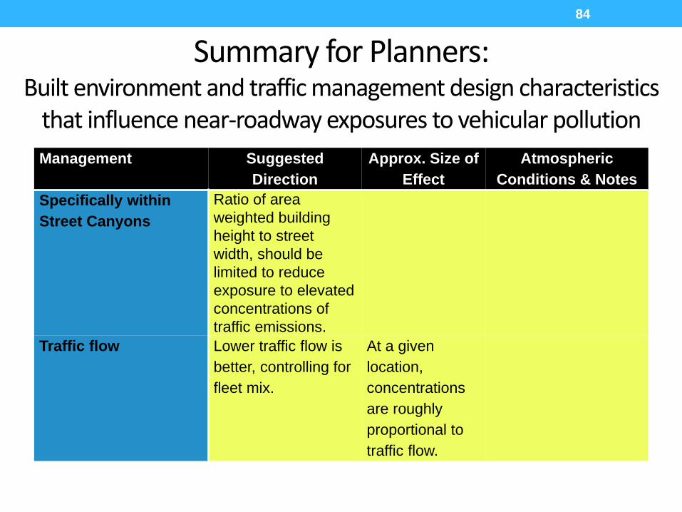
Summary for Planners: Built environment and traffic management design characteristics

that influence near-roadway exposures to vehicular pollutionManagement Suggested

DirectionApprox. Size of

EffectAtmospheric

Conditions & NotesSpecifically within Street Canyons

Ratio of area weighted building height to street width, should be limited to reduce exposure to elevated concentrations of traffic emissions.

Traffic flow Lower traffic flow is better, controlling for fleet mix.

At a given location, concentrations are roughly proportional to traffic flow.

84

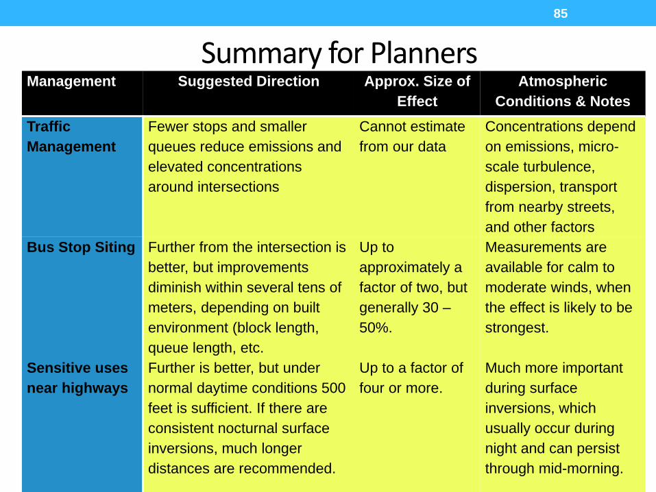
Summary for PlannersManagement Suggested Direction Approx. Size of

EffectAtmospheric

Conditions & NotesTraffic Management

Fewer stops and smaller queues reduce emissions and elevated concentrations around intersections

Cannot estimate from our data

Concentrations depend on emissions, micro-scale turbulence, dispersion, transport from nearby streets, and other factors

Bus Stop Siting Further from the intersection is better, but improvements diminish within several tens of meters, depending on built environment (block length, queue length, etc.

Up to approximately a factor of two, but generally 30 –50%.

Measurements are available for calm to moderate winds, when the effect is likely to be strongest.

Sensitive uses near highways

Further is better, but under normal daytime conditions 500 feet is sufficient. If there are consistent nocturnal surface inversions, much longer distances are recommended.

Up to a factor of four or more.

Much more important during surface inversions, which usually occur during night and can persist through mid-morning.

85

The People Who Really Did the Work:Dr. Wonsik ChoiDilhara RanasingheProf. J.R. DeShazoLisa Wong

CARB:Dr. Kathleen KozawaSteve MaraDr. Toshi Kuwayama

Supported by the California Air Resources Board, and the National Science Foundation

86

Dr. Shishan HuKaren BunavageDr. Rodrigo Siguel (UTAM, Chile)Prof. Arthur WinerProf. Mario GerlaProf. Brian Taylor

Si Tan Prof. Akula Venkatram

Thank you for your attention

87

Documents

Suzanne Paulson* & Nico Schulte** · IDENTIFYING URBAN DESIGNS AND TRAFFIC MANAGEMENT STRATEGIES FOR SOUTHERN CALIFORNIA THATREDUCE AIR POLLUTION EXPOSURE. Suzanne Paulson* & Nico