Embed Size (px)
Citation preview

Sustainable Engineering
Internship 2017 Final Report
July 16, 2017
Leah Balkin, Adrian D’Orlando, Sarah Jakositz, Eesha Khanna

SEI 2017 Final Report | 2
Table of Contents
Table of Contents 2
List of Figures 4
List of Tables 6
Executive Summaries 8
Assignment 1: Effectiveness of Hydrophobic Coating on Solar Panels 11
1.1 Background 11
1.2 Purpose 12
1.3 Scope 12
1.4 Methods 12
1.5 Results and Analysis 14
1.6 Conclusions and Recommendations 22
1.7 References 24
Assignment 2: Research Vessel Design/Technologies 25
2.1 Background 25
2.2 Purpose 25
2.3 Scope 25
2.4 Methods 25
2.5 Results and Analysis 27
2.6 Conclusions and Recommendations 30
2.7 References 31
Assignment 3: Electrical Grid- Master Plan 32
3.1 Background 32
3.2 Purpose 33
3.3 Scope 33
3.4 Methods 33
3.5 Results and Analysis 37
3.6 Conclusions and Recommendations 44
3.7 References 44
Assignment 4: Rooftop Water for Flushing Toilets and Watering Celia’s Garden 45
4.1 Background 45
4.2 Purpose 45
4.3 Scope 46
4.4 Methods 46
4.5 Results and Analysis 48
4.6 Conclusions and Recommendations 62
4.7 References 63

SEI 2017 Final Report | 3
Assignment 5: Lifespan Analysis of the Green Grid Batteries 64
5.1 Background 64
5.2 Purpose 64
5.3 Scope 64
5.4 Methods 64
5.5 Results and Analysis 67
5.6 Conclusions and Recommendations 77
5.7 References 77
Assignment 6: Using Rooftop Water for Additional Showers 78
6.1 Background 78
6.2 Purpose 78
6.3 Scope 78
6.4 Methods 78
6.5 Results and Analysis 81
6.6 Conclusions and Recommendations 83
6.7 References 84
Assignment 7: New Grease Trap Effectiveness 85
7.1 Background 85
7.2 Purpose 85
7.3 Scope 85
7.4 Methods 85
7.5 Analysis and Results 88
7.6 Conclusions and Recommendations 90
7.7 References 90
Assignment 8: Assessment of SML Groundwater Supply Well and Surrounding Point
Wells 91
8.1 Background 91
8.2 Purpose 91
8.3 Scope 91
8.4 Methods 91
8.5 Results and Analysis 95
8.5.6 Survey Data 100
8.6 Conclusions and Recommendations 101
8.7 References 103
Future Project Suggestions 104

SEI 2017 Final Report | 4
List of Figures
Figure 1. Uncoated panels before (a.) and after (b.) rain ............................................................................ 14
Figure 2. Average Daily Output for Coated and Uncoated Panels After Coating was Applied ................. 15
Figure 3. Average Daily Output for Coated and Uncoated Panels Before Coating was Applied ............... 16
Figure 4. Difference in Average Outputs and Solar Irradiance .................................................................. 17
Figure 5. Cleanliness of coated and uncoated panels after rain simulation ................................................ 21
Figure 6. MREU set-up ............................................................................................................................... 33
Figure 7. DOD vs Number of Cycles provided by manufacturer ............................................................... 41
Figure 8. Current generator load and load with MREU in place ................................................................ 43
Figure 9. Force breaker ............................................................................................................................... 53
Figure 10. Toilet survey that was distributed in Bartels Hall and Founder’s Hall from June 23rd to July
7th, 2017 ..................................................................................................................................................... 54
Figure 11. Rooftop measurements for Founder’s Hall. Note that the area highlighted in yellow is the
designated collection area ........................................................................................................................... 57
Figure 12. Picture of the basement of Founder’s Hall. To the right of the pole is the concrete slab that
could hold water storage tanks .................................................................................................................... 59
Figure 13. Picture of the existing cistern in the basement of Founder’s Hall ............................................. 59
Figure 14. To-scale graphic showing the proposed storage tank layout on the concrete slab in the
basement of Founder’s Hall. These tanks could hold 650 gallons (Jakositz 2017) .................................... 60
Figure 15. To-scale graphic showing the existing cistern in the basement of Founder’s Hall. This cistern
has a volume of 2100 gallons (Jakositz 2017) ............................................................................................ 60
Figure 16. Graphical depiction of a cycle, V .............................................................................................. 65
Figure 17. Graphical depiction of a cycle, Ah ............................................................................................ 66
Figure 18. Cycles of a battery over the course of four weeks ..................................................................... 67
Figure 19. Depiction of sudden spikes and drops in voltage ...................................................................... 68
Figure 20. Example of incomplete charging ............................................................................................... 69
Figure 21. Example of a mid-cycle drop to 0V ........................................................................................... 69
Figure 22. Example of multiple cycles in one day ...................................................................................... 70
Figure 23. Figure provided by manufacturer depicting number of cycles vs. depth of discharge .............. 72
Figure 24. Sample day in which the state of charge of the batteries fell to about 42% .............................. 75
Figure 25. Proposed location for the outdoor shower/rinsing station in red beside the Dive Locker ......... 79
Figure 26. Calculated dimensions and area of the proposed Kiggins Commons rooftop collection area ... 80
Figure 27. Additional three-gallon showers provided by the proposed system for average monthly rainfall
(a.) and low monthly rainfall (b.) ................................................................................................................ 82
Figure 28. 2016 interceptor coring sample (a.) and 2017 interceptor coring sample (b.) ........................... 86
Figure 29. 2017 coring sample of effluent (a.) and 2016 coring sample of effluent (b.) ............................ 87
Figure 30. Levelogger that was used to read water level data in each of the wells .................................... 92
Figure 31. Set-up for the slug and pump tests at the six-foot well .............................................................. 94
Figure 32. Water levels measured in feet above the mean tide level of the main well and six-foot well
from June 15th, 2017 to July 10th, 2017 ..................................................................................................... 95
Figure 33. Water levels measure in feet above mean tide level of the main well and six-foot well from
June 5th, 2017 to July 10th, 2017 ............................................................................................................... 96

SEI 2017 Final Report | 5
Figure 34. Water levels measured in feet above mean tide level of the main well and the Grass Lab well
from June 5th, 2017 to July 10th, 2017 ....................................................................................................... 97
Figure 35 a, b. Water levels measured in feet above mean tide level of the main well (a.) and Grass Lab
well (b.) from June 5th, 2017 to July 10th, 2017 ........................................................................................ 98
Figure 36. Temperature profile of main well, taken once from the top to bottom of the well (blue) and
once from the bottom to the top of the well (red) ....................................................................................... 99
Figure 37. Conductivity profile of the main well, taken once from the top to the bottom of the well (blue),
and once from the bottom to the top of the well (red) .............................................................................. 100
Figure 38. Survey measurements for each well on Appledore Island, June 27th, 2017 ........................... 101
Figure 39. Diagram of the main supply well location above the mean tide level. The freshwater lens is
also shown below the MTL line. Not that this is not to scale ................................................................... 102

SEI 2017 Final Report | 6
List of Tables
Table 1. Average power output for selected arrays ..................................................................................... 16
Table 2. Percentage of sunny days before and after coating was applied ................................................... 18
Table 3. Output Difference vs. Rainfall ...................................................................................................... 19
Table 4. Flow rates of high and low intensity rain simulations .................................................................. 20
Table 5. Percent cover and output for panel types before and after rainfall ............................................... 22
Table 6. Vessel needs and wants of SML staff ........................................................................................... 27
Table 7. Sample K-T Analysis template for evaluating hull material alternatives ..................................... 28
Table 8. Sample Pro-Con form for engine types......................................................................................... 29
Table 9. Sample vessel comparison table for JMK vs. UNH Gulf Challenger ........................................... 30
Table 10. Battery calculations spreadsheet sample ..................................................................................... 36
Table 11. Readings used to determine the running load for the saltwater pump ........................................ 38
Table 12. Overall measurements for the running load of the saltwater pump ............................................ 38
Table 13. Readings taken for the start-up load of the saltwater pump ........................................................ 38
Table 14. Efficiencies of each component of the MREU system ............................................................... 39
Table 15. Battery lifespan calculations based on manufacturer specs ........................................................ 41
Table 16. Voltage and current per string and per charge controller ............................................................ 42
Table 17. Data used for generator load decrease calculations .................................................................... 43
Table 18. Table of values collected from the water meter and the cistern in the basement of Bartels Hall
from June 23rd, 2017 to July 8th, 2017. ..................................................................................................... 49
Table 19. Power and energy calculations based on measured voltage, current, and time data taken from
the 0.5 horsepower pump in the basement of Bartels Hall ......................................................................... 50
Table 20. Well and cistern pump energy required to pump average daily water usage of Bartels Hall ..... 51
Table 21. Energy and cost increase of pumping water from Bartels Hall basement cistern compared to
pumping from well with original pumping system ..................................................................................... 52
Table 22. Monthly water and energy changes resulting from new rooftop rainwater collection, storage and
distribution system in Bartels Hall .............................................................................................................. 52
Table 23. Calculated average gallons of water used per day in Bartels Hall and Founder’s Hall based on
survey data .................................................................................................................................................. 55
Table 24. Calculated average gallons of water used per day in Bartels Hall and Founder’s Hall based on
Bartels Hall water meter data. This data was deemed to be more accurate than the data from table e, and
thus was used in further calculations .......................................................................................................... 56
Table 25. Amount of rooftop rainwater available per month for May through August given an average
summer and an absolute low summer ......................................................................................................... 58
Table 26. Summary of the capital costs of building the new rooftop rainwater collection, storage, and
distribution system for Founder’s Hall ....................................................................................................... 61
Table 27. Summary of the monthly energy usage and cost to pump water from the basement of Founder’s
Hall to the rest of the building .................................................................................................................... 62
Table 28. Results of graphical analysis for voltage and battery capacity ................................................... 71
Table 29. Calculated depth of discharge for the batteries ........................................................................... 71
Table 30. Percent of lifespan used and remaining each year ...................................................................... 72
Table 31. Projected number of years left in battery lifespan ...................................................................... 73
Table 32. Years of battery life permitted by various depths of discharge .................................................. 73

SEI 2017 Final Report | 7
Table 33. Reduction in battery lifespan due to various temperatures, provided by manufacturer .............. 74
Table 34. Ideal float voltage of battery system at various temperatures ..................................................... 76
Table 35. Approximate total equipment costs for the proposed system ..................................................... 83
Table 36. Pros and cons of three disposal options ...................................................................................... 89
Table 37. Summary of the ground elevation and top of casing elevation compared to mean tide level for
each well on Appledore Island, June 27th, 2017 ...................................................................................... 101
SEI 2017 Final Report | 8
Executive Summaries
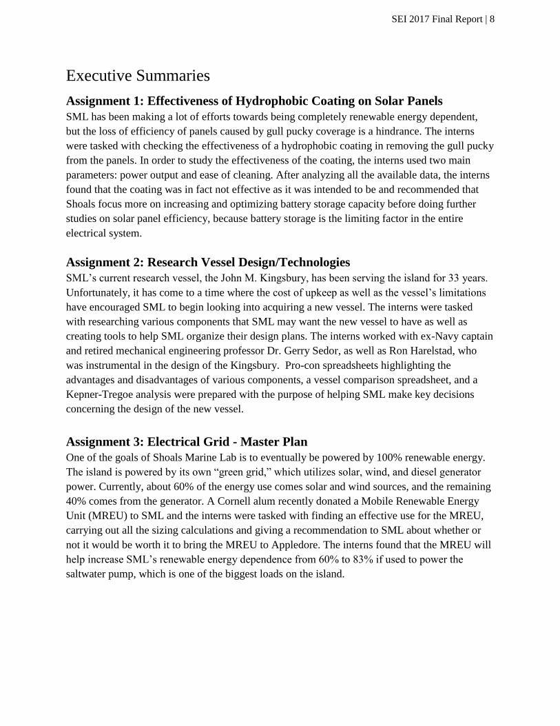
Assignment 1: Effectiveness of Hydrophobic Coating on Solar Panels
SML has been making a lot of efforts towards being completely renewable energy dependent,
but the loss of efficiency of panels caused by gull pucky coverage is a hindrance. The interns
were tasked with checking the effectiveness of a hydrophobic coating in removing the gull pucky
from the panels. In order to study the effectiveness of the coating, the interns used two main
parameters: power output and ease of cleaning. After analyzing all the available data, the interns
found that the coating was in fact not effective as it was intended to be and recommended that
Shoals focus more on increasing and optimizing battery storage capacity before doing further
studies on solar panel efficiency, because battery storage is the limiting factor in the entire
electrical system.
Assignment 2: Research Vessel Design/Technologies
SML’s current research vessel, the John M. Kingsbury, has been serving the island for 33 years.
Unfortunately, it has come to a time where the cost of upkeep as well as the vessel’s limitations
have encouraged SML to begin looking into acquiring a new vessel. The interns were tasked
with researching various components that SML may want the new vessel to have as well as
creating tools to help SML organize their design plans. The interns worked with ex-Navy captain
and retired mechanical engineering professor Dr. Gerry Sedor, as well as Ron Harelstad, who
was instrumental in the design of the Kingsbury. Pro-con spreadsheets highlighting the
advantages and disadvantages of various components, a vessel comparison spreadsheet, and a
Kepner-Tregoe analysis were prepared with the purpose of helping SML make key decisions
concerning the design of the new vessel.
Assignment 3: Electrical Grid - Master Plan
One of the goals of Shoals Marine Lab is to eventually be powered by 100% renewable energy.
The island is powered by its own “green grid,” which utilizes solar, wind, and diesel generator
power. Currently, about 60% of the energy use comes solar and wind sources, and the remaining
40% comes from the generator. A Cornell alum recently donated a Mobile Renewable Energy
Unit (MREU) to SML and the interns were tasked with finding an effective use for the MREU,
carrying out all the sizing calculations and giving a recommendation to SML about whether or
not it would be worth it to bring the MREU to Appledore. The interns found that the MREU will
help increase SML’s renewable energy dependence from 60% to 83% if used to power the
saltwater pump, which is one of the biggest loads on the island.

SEI 2017 Final Report | 9
Assignment 4: Rooftop Water for Flushing Toilets and Watering Celia’s
Garden
Freshwater is a precious resource on Appledore, and in order to conserve freshwater, SML
recently installed a rooftop rainwater toilet flushing system for Bartels Hall. The interns were
tasked with evaluating the water and energy savings for the rooftop water collection/delivery
system used for flushing toilets in Bartels Hall, designing a similar system for Founder’s Hall,
and designing a gravity-fed system to deliver supplementary rooftop water to Celia Thaxter’s
garden. The interns concluded that the Bartels System was working well and designed a similar
model for Founder’s Hall.
Assignment 5: Lifespan Analysis of the Green Grid Batteries
In 2014, SML installed a 300 kWh battery bank consisting of 40 absorbed glass mat (AGM)
batteries in green energy infrastructure improvements aimed at decreasing the generator running
time on the island. There was a learning curve in identifying the most efficient operational set
points for the system. Batteries are the weak link in the energy system and they will need to be
replaced first. SML wishes to make informed decisions about battery lifespan and maintenance
and therefore, the interns were tasked with conducting a cycle count for the batteries and
researching methods to help increase battery lifespan. The interns found that the batteries will
last for 13 more years if maintained properly. They also made some maintenance
recommendations, the most important one being proper temperature regulation.
Assignment 6: Using Rooftop Water for Additional Showers
SML wants to take advantage of freshwater sources like rainwater to allow the residents
additional showers. The interns were tasked with exploring the prospect of an outdoor shower in
terms of water treatment, greywater discharge, location of the shower, feasibility of a gravity-fed
system, and volume of rainwater collection. Due to the locational constraints for a typical
outdoor shower as well as strict regulations concerning the treatment of greywater, the interns
concluded that installing a rinsing station instead of a full shower or supporting the existing
shower system with rooftop collected water would be more feasible options.

SEI 2017 Final Report | 10
Assignment 7: New Grease Trap Effectiveness
In 2016, the Sustainable Engineering Interns evaluated the old grease trap behind Kiggins
Commons and found that it was not removing all the grease and solids before the stream entered
the piping that leads to the septic system. This led to the waste from the grease trap filling up the
septic tank and clogging the pipes. Therefore, the 2016 interns recommended that SML install a
new, larger grease trap that would be better equipped to handle the volume of grease from the
kitchen. On May 1st of 2017 the new grease trap was installed. This year’s interns were tasked
with evaluating the effectiveness of the new grease trap, making a maintenance schedule and
recommending disposal options for the collected grease. The interns found that the new grease
trap was working well and should be cleaned when the layer of grease is 6 inches thick. They
provided monitoring points for cleaning and also outlined the pros and cons of the different
disposal options that SML has.
Assignment 8: Assessment of SML Groundwater Supply Well and
Surrounding Point Wells
SML currently relies on a 22.5-foot deep well to support its freshwater demands. During dry
summers, SML has been forced to resort to using a reverse osmosis (RO) system to convert
saltwater to freshwater when the well supply is not enough. As a result, SML is actively
searching for new sources of freshwater. Last year, the 2016 SEI interns worked with Emery &
Garrett Groundwater Investigations (EGGI) to locate a potential location for a new well. This
year, the interns were tasked with determining if a well installed in this new location would be
hydraulically connected to the aquifer that the current main supply well is already pulling from.
Based on data that was obtained from Leveloggers and help from EGGI, the interns propose that
the new potential site is in fact connected to the current well’s groundwater source. However,
further investigations should be carried out to determine if there is another pocket of water
beneath the bedrock that limited the depth of the new test well.

SEI 2017 Final Report | 11
Assignment 1: Effectiveness of Hydrophobic Coating on Solar
Panels
Project Leads: Leah Balkin and Eesha Khanna
1.1 Background
On June 9th of 2017, a hydrophobic coating was applied to one array of solar panels at Shoals
Marine Lab. This coating was created by Alpha Nano Solutions and was donated to Shoals by
Professor Glenn Shwaery. It was originally formulated for desert conditions, and works to
increase solar output in dusty conditions while reducing cleaning frequency and the volume of
water needed to clean the panels. According to Alpha Nano Solutions, dust-free panels
consistently outperform dirty panels, and therefore, in order to achieve optimum output, it is vital
that they are maintained to the highest standard.
Being on a gull colony, the solar panels receive large amounts of gull feces, referred to by island
residents as “pucky.” This is especially true for panels on the roofs, because gulls are attracted
to heights. Past SEI reports have shown that the coverage caused by gull pucky affects the output
of the panels. Therefore, the coating was applied to one of the arrays to test whether it assisted
cleaning of the panels during rainfall and whether this was reflected in the panel output.
Ideally, the coating should be applied on new panels, not used ones. It needs to be applied before
the panels are put in use so there is a clean, pristine surface. That was not the case when it was
applied on the panels at SML. The panels had never been cleaned since they were installed and
they had to be scraped and thoroughly cleaned before the coating was applied. There were small
residues still left on the panels even after cleaning them. Moreover, the panels cannot be exposed
to water and need to be kept in a specific temperature range for 24 hours after the coating is
applied. The panels were covered with plastic sheets to prevent the gulls and rain from going on
them for 24 hours, however, the panels were exposed to rain before 24 hours were over since the
wind blew the coverings off the panels. The way the coating was applied was not ideal at all and
that could also contribute to the lifespan/effectiveness of the coating.
The arrays that were tested were on the Pole Barn. The coated array was comprised of the top
two rows and the uncoated array was comprised of the bottom two rows. This setup was not ideal
because the gulls are most attracted to the highest point of the roof, thereby leading to more
pucky on the top panels compared to the bottom panels. This inherent inequality in pucky cover
between the panels is a factor that could skew the results, but the interns accounted for that.

SEI 2017 Final Report | 12
1.2 Purpose
The coating costs $400 for 6 ounces and has a warranty for two years. Professor Glenn Shwaery
donated 250 milliliters of the coating, which has a value of $560. 120 mL of the donation was
used to coat one array. The 2017 interns were tasked with evaluating whether or not the coating
is worth investing in for all the solar panels on Appledore Island.
1.3 Scope
The interns used 3 different methods to analyze the effectiveness of the hydrophobic coating:
comparison of power output for coated and uncoated arrays as well as for coated array before
and after the coating was applied; comparison of change in percent cover after rainfall for coated
and uncoated array; and comparison of the reaction to a simulated rainfall for coated and
uncoated arrays. The interns also did a cost-benefit analysis and were able to come to a
conclusion.
1.4 Methods
1.4.1 Power Output
The coating was applied to array 8 (the top array on Ross’s Pole Barn) on June 9, 2017, and
array 9 (the bottom array on Ross’s Pole Barn) was used as a control. Both arrays were left
covered for one day as the coating dried on array 8 and the covers were removed on June 10,
2017 around 10 am. The output data for these 2 arrays started recording June 2 onwards (one
week before the coating was applied). The output data from June 2 - July 10 was collected from
the ComBox system in the Energy Conservation Building. Pyranometer data, which measures
solar irradiance, was also collected for the same dates. This allowed the interns to track solar
intensity and correct for discrepancies in outputs due to differences in solar intensity on different
days. It is important to note that one of the limitations of this project was the lack of output data
available for arrays 8 and 9 before the coating was applied.
The interns created a spreadsheet for this data and calculated the difference in average and total
outputs for arrays 8 and 9 before and after the coating was applied. The outputs for arrays 8 and
9 were graphed to see how they changed after the coating was applied. The solar irradiance was
also graphed with the outputs in order to ensure that the power output each day matched the
amount of energy available. In addition, the difference in power output between the two panels
was calculated and graphed over the 24 day period. This graph was analyzed to see if a
significant difference in output was evident after the coating was applied.

SEI 2017 Final Report | 13
1.4.2 Simulated Rainfall
With the help of Bob Austin, an island engineer, the interns performed two different trials of
stimulating a rainfall event to look qualitatively at how the coating affects the removal of gull
pucky.
For the preliminary trial, both the coated (8) and uncoated (9) arrays were sprayed down with the
hose at high intensity to get a general idea of how easily they could be cleaned. The mobility of
the gull pucky was observed while the two arrays were being washed down and a qualitative
assessment was made.
For the second trial the interns chose four coated panels and paired them with four uncoated
panels that had relatively the same amount of gull pucky coverage. Two different intensities of
rain were tested: low intensity and high intensity. Each intensity was tested on two different pairs
of coated/uncoated panels. The low intensity trial was more realistic and compared to real
rainfall, while the high intensity trial compared to cleaning the panels with a hose. The interns
timed how long it took to remove the gull pucky off each of the panels. Additionally, the flow
rates for the high intensity and low intensity trials were calculated by timing how long it took to
fill a five-gallon bucket. The flow rates were calculated to assist with volume calculations. The
volume of water that was required to clean each panel was calculated and the numbers were
compared.
1.4.3 Percent Cover Before and After Rainfall
The interns decided to take pictures of the coated and uncoated panels before and after rainfall
events to see how the percent cover change differed for the coated and uncoated panels.
However, they faced some difficulty setting up a system that would allow them to capture such
pictures. Pictures taken by the webcam and from the deck at Kiggins Commons were not clear
enough to analyze such details. With the help of John Durant, the interns set up a ladder that
went up to the Pole Barn roof and climbed up the ladder to take pictures. Since the roof does not
have any free space available, the interns were not able to get on top, and only managed to get
pictures for one side of the roof. Therefore, it was decided that pictures of one coated and one
uncoated panel would be analyzed and the result would be extrapolated. While this method was
not ideal, it was accurate as the surrounding panels behaved similarly (based on observations and
pictures taken).
Pictures of one coated panel and one uncoated panel were taken before a rainfall event. After it
rained, pictures of the same two panels were taken again. Pictures were taken of both panels at
multiple different angles to avoid the glare of the sun and to ensure that the entire panel could be
clearly seen. This helped the interns to effectively calculate the percent cover.

SEI 2017 Final Report | 14
a. b.
Figure 1. Uncoated panels before (a.) and after (b.) rain
Using these pictures, such as the ones shown in Figure 1, the interns found the percent cover for
the uncoated and coated panels both before the rainfall and after. In order to find the percent
cover, the interns tried using an online color percent calculator, but the fact that the gull to give
inaccurate results. The interns then projected the solar panels on excel, with each excel cell
representing a solar cell. The percent cover for each cell was estimated and these were added up
and scaled to calculate the percent cover. The results were then analyzed and compared to see
how the percent cover changed for the coated and uncoated panels.
1.5 Results and Analysis
1.5.1 Power Output
1.5.1.1 Power Output Difference
The power output of the coated array (8) and the uncoated array (9) from June 2nd to July 10th
was plotted. Solar irradiance data for this time period was also plotted alongside the power
output graphs in order to ensure the panels output matched the amount of solar energy available.
The interns noted that the coated array had a higher average output than the uncoated array even
before the coating was applied. Therefore, the key part of the analysis was based on how the
difference in outputs for arrays 8 and 9 changed after the coating was applied, because this
difference allowed the interns to correct for variation due to solar irradiance difference on
different days, and for inherent difference in array efficiencies.
There could be many factors that account for this inherent difference in output. For example,
array 9 could be more worn out than array 8 resulting in decreased ability to capture solar

SEI 2017 Final Report | 15
energy. There could be more line losses for array 9, resulting in less power being captured as it
travels from the panels to the charge controllers in the Energy Conservation Building, or there
could be manufacturing differences in efficiencies. The exact cause of this difference is beyond
the scope of this project but is taken into consideration.
The average power output each day was graphed for the two arrays starting June 9th, when the
coating was applied.
Figure 2. Average Daily Output for Coated and Uncoated Panels After Coating was
Applied
From this graph it is evident that the coated array is outperforming the uncoated array most days
after the coating was applied. Next the average output of the two arrays before the coating was
applied was graphed.

SEI 2017 Final Report | 16
Figure 3. Average Daily Output for Coated and Uncoated Panels Before Coating was
Applied
From this graph it is evident that the coated array was outperforming the uncoated array even
before the coating was applied.
Additionally, from the output data, the average power output for each array was calculated
before and after the coating was applied.
Table 1. Average power output for selected arrays
Time Period Array 8 (Coated) Array 9 (Uncoated)
6/2 - 6/8 443.6 kW 368.4 kW
6/10 - 6/26 654.2 kW 542.8 kW
Difference in average outputs before coating was applied: 75.2 W
Difference in average outputs after coating was applied: 103.42 W
From this table, it can be seen that there is a 37% percent increase in difference between average
outputs for arrays 8 and 9 since the coating has been applied. However, due to the
SEI 2017 Final Report | 17
outperformance of the coated array before and after coating, the interns were skeptical of this
37% increase.
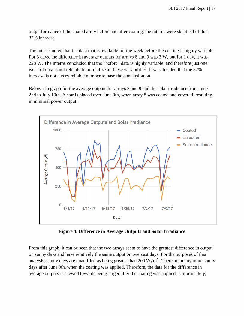
The interns noted that the data that is available for the week before the coating is highly variable.
For 3 days, the difference in average outputs for arrays 8 and 9 was 3 W, but for 1 day, it was
228 W. The interns concluded that the “before” data is highly variable, and therefore just one
week of data is not reliable to normalize all these variabilities. It was decided that the 37%
increase is not a very reliable number to base the conclusion on.
Below is a graph for the average outputs for arrays 8 and 9 and the solar irradiance from June
2nd to July 10th. A star is placed over June 9th, when array 8 was coated and covered, resulting
in minimal power output.
Figure 4. Difference in Average Outputs and Solar Irradiance
From this graph, it can be seen that the two arrays seem to have the greatest difference in output
on sunny days and have relatively the same output on overcast days. For the purposes of this
analysis, sunny days are quantified as being greater than 200 W/m2. There are many more sunny
days after June 9th, when the coating was applied. Therefore, the data for the difference in
average outputs is skewed towards being larger after the coating was applied. Unfortunately,

SEI 2017 Final Report | 18
there was not enough data available to normalize this trend. This means that the 37% increase in
percent difference is likely unreliable.
Also, the trend for increased power output for array 9 is evident both before and after the coating
is applied. This inherent difference in the power output of the two panels that is important to
note.
In addition, the interns looked at the percentage of sunny days both before and after the coating
was applied to make sense of the difference in output data.
Table 2. Percentage of sunny days before and after coating was applied
Before Coating After Coating
Number of Days above 200𝑊/𝑚2 5 27
Number of Days below 200𝑊/𝑚2 2 4
Percent Sunny Days 71% 87%
There was a 16% increase in sunny days after the coating was applied. Since it has been shown
that the array 8 has always had a greater output on sunnier days, this 16% increase is a factor that
affects the 37% increase in the difference in average power output after the coating was applied.
1.5.1.2 Power Output vs Rainfall
Analyzing average output data was not enough to make a conclusion on the effectiveness of the
coating because the effects of rainfall only last for a day or two before the panels are soiled
again. Also, if the coating is effective in removing gull pucky after rainfall, the interns felt that
this should be reflected in the power output and tried to verify this hypothesis. The interns
specifically looked at days when it rained and since it mostly finished raining in the
evening/night, they analyzed the data for the next day. The following table shows rainfall data
and output data for days when it rained in the time period of the experiment. Solar irradiance was
also checked to make sure the day was sunny and that it did not contradict the previous claim
about sunny days giving a higher difference.

SEI 2017 Final Report | 19
Table 3. Output Difference vs. Rainfall
Even though there is not enough “before” data to make a solid conclusion, it can be seen that the
difference in outputs was higher before the coating was applied. Particularly looking at days
when it rained approximately the same amount (6/6/17 and 6/16/17, 6/7/17 and 6/27/17), it was
found that the difference was greater before the coating was applied. Even though Solar
Irradiance was higher on both the before days, the interns still think this analysis gives
contradictory results and invalidates the claim that power output strictly increases with coating.
There are variations that cannot be accounted for. For instance, the data only shows how much it
rained, not how it rained, but despite these variations, the results from this table were enough to
highlight the need for more data. This table is not enough to say that power output difference
decreases due to the coating, but it enough to doubt the claim that it increases due to the coating,
and to prevent the interns from making a decision in favor of the coating.
1.5.2 Simulated Rainfall
The preliminary simulated rainfall experiment was a qualitative assessment of the mobility
observed on the panels when they were being washed down. The interns observed that panels
with the coating allowed for more mobility of the gull pucky as they were being washed down.
The difference in mobility was clearly visible and the amount of time and water it took to wash
the coated panels was lower for the coated panels. The water was also beading up on the coated
panels, thereby indicating hydrophobicity.
The second simulated rainfall experiment was a quantitative assessment of the volume of water
needed to clean the coated and uncoated panels. Before the experiment could be conducted, the

SEI 2017 Final Report | 20
flow rates for the low and high intensity rainfalls had to be determined. The interns computed the
flow rates by timing how long it took to fill a 5 gallon bucket at the two different intensities.
Table 4 lists the flow rates. It is important to note that the difference in flow rates led to a
difference in the force of the water. The high intensity flow rate was more concentrated and
forceful.
Table 4. Flow rates of high and low intensity rain simulations
Low intensity High intensity
Time taken (s) 149 92
Flow rate (gallons/minute) 2.01 3.26
For the low intensity trial, two coated and two uncoated panels were selected. The uncoated
panels were sprayed for an average of 83 seconds using up 2.78 gallons of water and a
substantial amount of gull pucky was still left on the panels. The coated panels were sprayed for
an average of 73.5 seconds using up 2.47 gallons of water and a small amount of gull pucky was
still left on the panels.
For the high intensity trial, two coated and two uncoated panels were selected. The uncoated
panels were sprayed for an average of 71.5 seconds using up 3.89 gallons of water and a small
amount of gull pucky was still left on the panels. The coated panels were sprayed for an average
of 38.5 seconds, using up 2.09 gallons of water and no visible gull pucky was left on the panels.

SEI 2017 Final Report | 21
Figure 5. Cleanliness of coated and uncoated panels after rain simulation
++ implies that a substantial amount of gull pucky was left on the panels
+ implies that a small amount of gull pucky was left on the panels
It is important to note that some of the gull pucky on the panels was fresh while the rest was aged
and baked under the sun. This difference in age of pucky would affect how much water would be
needed to remove it, as the aged pucky was more difficult to remove. This is a factor that could
not be accounted for in this experiment.
After analyzing the results for the low intensity rainfall, it was found that neither the coated
panels, nor the uncoated panels were completely clean at the end of the experiment, but the
coated panels were relatively cleaner than the uncoated. The difference in volume of water
needed was not a large amount (0.3 gallons), therefore, implying that the low intensity rainfall
was not very effective, even with the coating. The difference in volume of water needed for the
high intensity trial was 1.8 gallons and the coated panels were significantly cleaner as there was
no gull pucky left on them, while there was a small amount left on the uncoated panels. The high
intensity rainfall was more effective in cleaning the coated panels, as it used the least amount of
water and the panels had no visible pucky left on them. However, this intensity does not
represent a realistic, average rainfall.
Based on the volume of water used to clean the coated and uncoated panels, the interns
calculated the volume of water that would be saved if SML decided to clean the panels on a
regular basis. The total number of solar panels was counted by the interns. It was found that there

SEI 2017 Final Report | 22
are 232 solar panels, excluding the ones on the roof of Kiggins Commons as those are passive
heating panels that do not contribute to any of the grids. The following calculation was done:
● Volume of water saved per panel = 1.8 gallons
● Total volume of water saved per round of cleaning = 1.8 gallons/panel x 232 panels =
417.6 gallons
It is important to note that this calculation is based on an average percent coverage, and that the
amount of water used can vary depending on how high the percent coverage is.
1.5.3 Percent Cover Before and After Rainfall
By analyzing pictures of one coated and one uncoated panel before and after a rainfall event, the
difference in percent cover on the panels was calculated before and after the rain and the
difference in power output was found for these times (Table 5).
Table 5. Percent cover and output for panel types before and after rainfall
Panel % Cover
Before
% Cover
After
% Cover
Difference
Output
Before (W)
Output
After (W)
Output %
Difference
Coated 3.4 1.25 2.15 2557 2616 +2.3
Uncoated 2.14 0.54 1.6 2613 2598 -0.5
The coated panels had a 35% greater percent cover difference than the uncoated panels. The
difference in percent cover was expected, as the panel with the hydrophobic coating had less
pucky coverage after the rain compared to the panel without the coating. Therefore, it is evident
that the coating does its job in keeping the panels clear of gull pucky. The more important
question that needs to be answered, however, is whether or not this percent cover change is large
enough for a significant change in solar output. However, the data collected for the power output
before and after the rainfall event is very subjective because it depends on cloud cover. As a
result, this experiment does not offer a good answer to whether the change in output is
significant.
1.6 Conclusions and Recommendations
Overall, two parameters were considered when deciding whether or not the coating is worth the
cost. These parameters were:
● Effect of coating on power output
● Effect of coating on ease of cleaning.
After going through all of the experiments, the interns realized that the power output data was
not a true indicator of the effectiveness of the coating because power output is affected by
several other factors like sunlight intensity, inherent efficiency of panels, etc. Therefore, it was

SEI 2017 Final Report | 23
decided that the second parameter will be given more weight when analyzing the results and
making a recommendation.
From method 1, the interns drew two conflicting conclusions. There was an increase in
difference between average outputs of coated and uncoated arrays after the coating was applied.
However, the part of the analysis that particularly looked at days when it rained led to the
conclusion that the difference in outputs was higher before the coating was applied. The interns
concluded that both of these results were not very reliable due to lack of data and influence of
several other variables that cannot be accounted for.
From method 2, it was concluded that the coating did prove to be effective in facilitating
cleaning of panels as the gull pucky was very mobile. The pucky easily came off the coated
panels, while the gully pucky on the uncoated panels did not come off completely even after
spraying for several minutes. Further, it was concluded that if SML was to regularly clean the
panels, the presence of the coating could reduce water usage.
From method 3, it was concluded that the coating worked to remove a greater percent of the gull
pucky from the panels when it rained by about 35%. The fact that this method was limited by
several factors was taken into account when analyzing the overall results.
Overall, the interns concluded that the coating was effective in removing the gull pucky more
easily when it rained or when the panels were sprayed. However, this result was not clearly
reflected in the power output data. The reason for this is perhaps the fact that SML never cleans
the panels and solely relies on rain for cleaning. Right after rain, the coated panels do get cleaner
than the uncoated panels, but within a day or so the panels are soiled again by the gulls. Other
reasons why the power output data did not clearly reflect the effectiveness of the coating could
be that there are either too many variables changing at all times or that the presence of the gull
pucky is in fact not significantly affecting output.
Since the effectiveness of the coating has been clearly visible only in ease of cleaning and SML
is looking for an increased output as a result of applying the coating, the interns feel that the
coating might prove to be worth its cost only if the panels are cleaned regularly (at least once a
week), in addition to cleaning by rain. However, SML does not currently clean any of the solar
panels and it is not realistic to expect them to budget in time each week to clean the panels,
especially since a conclusive answer as to if it will increase power output of the panels has not
been reached.
The lack of significant results from output data and the uncertainty caused by other variables as
well as the fact that the coating would require cleaning 232 panels every week to show any effect
led to the conclusion that the coating is not effective on Appledore Island. The interns

SEI 2017 Final Report | 24
recommend SML not to invest in the coating based on this year’s results. However, since the
time period of the experiment was just one month, the interns feel that their sample was not large
enough to normalize the variability in data. One possibility is to re-do the experiment next year
when more data is available, but the interns feel that there are more urgent issues that need to be
addressed first. The problem that SML currently has is finding enough battery storage for all the
available sun power. There is excess solar output that the arrays produce, but it cannot be
captured because of limitations in the battery storage capacity. Since there is not a shortage in
power output, the extra power that could potentially be gleaned from this coating would not
make much of a difference. Therefore, the interns recommend that SML look more deeply into
expanding battery storage on the island before finding ways to increase power output.
1.7 References
Glenn Shwaery (representative from Alpha Nanotechnology)
Alpha Nanotechnology (http://www.alphananosolutions.com)
Alex Brickett, UNH Facilities and Relief Island Engineer

SEI 2017 Final Report | 25
Assignment 2: Research Vessel Design/Technologies
Project Leads: Leah Balkin and Sarah Jakositz
2.1 Background
Shoals Marine Laboratory is in the early planning stages to replace its 47-foot research vessel,
the John M Kingsbury (JMK), with a new vessel. The Kingsbury has been a great vessel for
SML in that it has fulfilled their needs to transfer people, food, and cargo. However, SML feels
that the maintenance and upkeep of a 33-year old steel vessel along with its design and
equipment limitations is the driver for a replacement within a few years. This project begins
SML’s process of making decisions towards the acquisition of a new research vessel. These
decisions require preparation and planning to ensure that SML obtains a vessel of the best
possible design for their situation.
2.2 Purpose
There are many aspects that go into making a new vessel and, in SML’s case, many parties that
are invested in the design of the vessel. SML is beginning the process of determining what they
are looking for in a boat, and to help with this process the interns were tasked with designing a
method to assist SML in making key design decisions. The deliverables presented will facilitate
conversations on the design of the vessel and what will work best for SML as a whole.
2.3 Scope
The interns conducted research on research vessels similar to the Kingsbury and the different
alternatives available for a new vessel. Gerry Sedor, an ex-Navy Captain and retired UNH
professor, assisted the interns in designing a Kepner-Tregoe (K-T) analysis. The interns also
discussed advantages and disadvantages of various key design options with Ron Harelstad, who
was instrumental in designing the JMK. Ron educated the interns about the design of the JMK
and assisted in verifying their research deliverables for the Pro-Con analysis.
2.4 Methods
2.4.1 Needs and Wants
After speaking with Gerry Sedor, the interns learned that the most important first step in
designing a vessel is distinguishing needs from wants. A “need” is a criterion that must be
incorporated in the design. In SML’s case, this includes speed, lifespan, number of passengers,
etc. The “wants” are items that would be beneficial to the use of the vessel, but can be
overlooked should the design require compromises. When looking at different alternatives, if an
option does not satisfy the needs of the party, such as an engine that cannot support the required

SEI 2017 Final Report | 26
speed or a hull that cannot hold the necessary weight of cargo, then it should not be considered.
If an option meets the needs of SML, alternatives can then be judged on how they fulfill the
wants. The interns spoke with the island staff in order to make a preliminary list of needs and
wants.
2.4.2 Kepner-Tregoe Analysis
A K-T analysis is a method to organize, gather, prioritize, and analyze information in an
unbiased fashion. The steps are as follows:
1. Establish objectives
a. i.e. a hull material that will meet the needs of SML
2. Classify importance of design priorities
a. i.e. initial cost, maintenance cost, ease of maintenance, etc.
3. Generate alternatives to the objective
a. i.e. Aluminum, steel, etc.
4. Evaluate alternatives against the objective using weighted ratings
a. i.e. an item pertaining to safety regulations might be weighted at a 10 while cost
factors might be weighted at a 6
5. Sum scores for each alternative, taking weights into account
a. Alternative with the highest score is considered the “best” choice
2.4.3 Pro-Con
The interns created a document to provide background information in the form of pro-con tables
on various components of a vessel, including hull type, hull material, engine type, and propulsion
type. These were topics that SML specifically requested of the interns. This allows SML staff
who might not be as familiar with this topic to inform themselves of pertinent information and
contribute to the decision-making process. The interns worked closely with Ron Harelstad, who
was instrumental in the design of the John M. Kingsbury. He helped to verify the information in
the pro-con documents.
2.4.4 Comparable Vessels
The interns created a document of vessels that are comparable to the Kingsbury in size, capacity,
and function. The purpose of this was to look at aspects that the Kingsbury currently has or does
not have and analyze potential desired design options that already exist on other vessels in order
to determine what works and what does not. With this information, SML can look at other boats
to see what other options exist for the design of the new vessel. The interns created a spreadsheet
for SML that includes multiple vessels and an outline of each vessel’s specs.

SEI 2017 Final Report | 27
2.5 Results and Analysis
2.5.1 Needs and Wants
The interns created the following preliminary list of needs and wants for a research vessel. SML
can add to this list as discussion on the research vessel progresses. This list is a good basis for
SML to keep in mind what aspects of the boat are most pertinent as well as what options might
be expendable while designing.
Below is a preview of the needs/wants list that the interns created:
Table 6. Vessel needs and wants of SML staff
Needs Wants
5ft Draft Budget ($1.5-2M)
15,000 lb weight capacity Support diving activities
Crane Whale watch trips
20-30 year lifespan Seal trips
15 Knot cruising speed Trawling/dredging trips
Hold for food and luggage Chartering (i.e. for Docent Program
/ island tours)
+/- 50 ft length Shade and protection from heavy
weather
2.5.2 Kepner-Tregoe Analysis
The interns created a spreadsheet in excel for a preliminary K-T analysis template. In filling this
out, SML should consider their needs and wants and weigh their priorities on a scale of 1-10.
Then, they should fill out the spreadsheet and compare the scores of each option. The interns
made K-T analysis tabs in the spreadsheet for hull material, hull type, engine type, and
propulsion system. When the scores are entered into the cells depending on how important an
objective is to the wants of SML, the score automatically calculates for each option. Below is an
example of the hull material K-T analysis

SEI 2017 Final Report | 28
Table 7. Sample K-T Analysis template for evaluating hull material alternatives
Objectives
Hull material
Aluminum Steel Fiberglass
Needs
20-30 year lifespan
15 Knot cruising speed
Wants
Budget ($1.5-2M)
Sustainable
Low Maintenance
Total 0 0 0
2.5.3 Pro-Con
The interns researched different options for hull material, hull type, engine type, and propulsion
system. Then, these options were compiled in a spreadsheet and the interns researched the pros
and cons of each. Ron Harelstad checked over the interns’ work to ensure that the research found
was accurate. Here is a preview of the engine type pro-con sheet:

SEI 2017 Final Report | 29
Table 8. Sample Pro-Con form for engine types
Diesel Electric Diesel-Electric
Pros Cons Pros Cons Pros Cons
Durability Emissions Motor is
silent
Battery
storage/
energy
availability
Economic
More weight
than diesel
engine alone
More efficient
than gas
~$.59/nautical
mile
Not releasing
emissions
There are not
a lot to base
off of
High efficiency
across entire speed
range
Need room for
the batteries-->
less storage
Easy to use
Can corrode if
unused for the
winter (not a
problem if heat
exchangers are
installed)
~$.09/nautic
al mile
Cost
possibly?
Reduced
maintenance
Need to have
safety measures
in place to
avoid battery
explosions
Safety and
dependability
Not good for
long periods of
low rpms/idling,
etc.
Hybrid can
shift to
generator
when
batteries are
low
Lifespan of
the batteries
Reduction in
emissions
2.5.4 Comparable Vessels
The interns compiled research on specs of different vessels that are comparable to the JMK and
the new proposed vessel in capacity and function. The specs were compiled in a spreadsheet to
easily compare what the JMK has and options that are available and in use on other vessels.
Some cells are left blank as the interns were not able to find that information. Here is a preview
of the Gulf Challenger compared with the JMK:

SEI 2017 Final Report | 30
Table 9. Sample vessel comparison table for JMK vs. UNH Gulf Challenger
John M. Kingsbury SML R/V Gulf Challenger UNH
Length 46 ft 50 ft
Beam 25 ft 16 ft
Draft 5 ft 5 ft
Working deck 240 sq ft
Cruising 8 knots 18 knots
Range
Fuel Capacity 1100 gal
Portable Water 325 gal
Endurance 3 days
Passengers 48 39
Hull material Aluminum
Engine Diesel
Diesel; Twin Caterpillar C-
12 ACERT Compact
Cargo Load/Weight Displacement = 25 tons
2.6 Conclusions and Recommendations
The interns recommend that SML utilize the different methods for organizing the decision-
making process and adjust the documents according to their changing needs. Once SML has a
clear idea of the needs and wants for the new vessel, they can hold a charrette with the interested
parties to talk about the construction and the design process can follow.
From the pros and cons of different alternatives for the boat, the interns have created
recommendations based on conversations with Ron Harelstad as well as extensive internet
research. The interns feel that aluminum would be a suitable hull type as many new similar
vessels have aluminum hulls and it is lightweight, easy to weld, requires low maintenance, and
can be recycled at the end of the boat’s lifespan. In addition, after discussing with Ron Harelstad,
they recommend a semi-displacement hull for speed and efficiency and an azipod prop for
maneuverability. The interns also recommend that SML look further into a hybrid diesel-electric

SEI 2017 Final Report | 31
engine in order to reduce emissions and maintenance costs. Furthermore, the interns recommend
that SML look into Coast Guard boat design requirements throughout the process to ease
decision process and ensure that the vessel fulfills Coast Guard standards.
2.7 References
Devault, Robert T. "The Basics of Jet Propulsion." Trailer Boats. N.p.: n.p., n.d. 33-35. Print.
"Catamarans - Monohulls: Pros and Cons." Sailonline.com. N.p., 16 July 2017. Web. 16 July
2017.
Bareboats BVI. "Catamaran Vs. Monohull - How to Choose?" Bareboat Yacht Charters in the
British Virgin Islands. N.p., n.d. Web. 16 July 2017.
Boat Pennsylvania Course. "Hull Types and How They Operate." Official State Boater License
Courses. Kalkomy, n.d. Web. 16 July 2017.
Falvey, Kevin. "Catamaran Versus V-Hull: Which Rides Better?" Boating Magazine. Boating, 2
Dec. 2004. Web. 16 July 2017.
Glen-L Marine Designs. Boatbuilding 101. Rep. N.p.: n.p., n.d. Print.
Gorsuch, Chris. "Inboard vs. Outboard Jet Drives." Pennsylvania Angler & Boater. N.p., n.d.
Web. July 2011.
Hamilton Jet, comp. Jet Torque from Hamilton Jet. Tech. N.p.: n.p., n.d. June 2002. Web. 16
July 2017.
Kasten, Michael. "METAL BOATS." Metal Boats For Blue Water - Kasten Marine Design.
Kasten Marine Design, n.d. Web. 16 July 2017.
MAN, comp. Diesel-electric Drives. Tech. n.p., n.d. Web. 16 July 2017.
Nordhaven. "Hull Design." Nordhaven. N.p., n.d. Web. 16 July 2017.
Parkinson, Andrew. "Sailboat Debate: Monohull vs. Catamaran." Yachts International. N.p., 17
Aug. 2015. Web. 16 July 2017.
Powerboat Training NZ. "Fiberglas Versus Aluminium Boats." Blog post. Pros And Cons Of
Choosing An Aluminium Or Fiberglass Boat. N.p., 9 Jan. 2013. Web. 16 July 2017.
Ron Harlstad (designed the Kingsbury)
Rudow, Lenny. "Outboards, Inboards, Pod Drives, Stern Drives, and Jets: Which Is the Best?"
Boats.com. N.p., n.d. Web. 12 July 2014.
Thomas, Tim. "A Guide to Superyacht Hull Design." Boat International. N.p., 21 Jan. 2015.
Web. 16 July 2017.
"Types of Hulls." Takemefishing.org. N.p., n.d. Web. 16 July 2017.
Yachting Pages. "Aluminium Boat Hulls VS Steel Boat Hulls." Yachting Pages. N.p., 4 May
2017. Web. 16 July 2017.
"Yacht Hull Types." Outer Reef Yachts. N.p., n.d. Web. 16 July 2017.
Brewer, Ted. "Is There a Metal Yacht in Your Future?" Good Old Boat. N.p., 4 July 1999. Web.
16 July 2017.

SEI 2017 Final Report | 32
Assignment 3: Electrical Grid- Master Plan
Project Leads: Adrian D’Orlando and Eesha Khanna
3.1 Background
One of the goals of Shoals Marine Lab is to eventually be powered by 100% renewable energy.
The island is powered by its own “green grid,” which utilizes solar, wind, and diesel generator
power. Typically, the combination of solar and wind power are able to supply the island’s needs
for a majority of the day, and also charge the two battery banks that are located in the Energy
Conservation Building (ECB) and the radar tower. However, the generator must run every night
after the stored battery energy is depleted. Currently, about 60% of the energy use comes solar
and wind sources, and the remaining 40% comes from the generator. On most days, the island’s
wind turbine and 232 solar panels produce more energy than can be stored by the batteries, so the
limitation that the island faces is not due to a lack of ability to generate green energy but rather a
lack of ability to store enough of it to make it through the night.
Two of the biggest energy loads on the island are coming from the saltwater pump and from
Kiggins Commons, which contains the kitchen, dining area, research labs, and the water
conservation building. Removing or reducing one of these loads may be essential in achieving
the goal of making it through the night without the generator.
SML received a Mobile Renewable Energy Unit (MREU) designed by Florida Solar Energy as a
donation from Sean O’Day, a Cornell alum. The MREU is a compact, mobile energy generation
and storage system that consists of 100 monocrystalline solar panels that have a 30 kW capacity,
a 76.4 kWh Lithium “Never-Die” battery bank, 10 Schneider Electric charge controllers and 7
Schneider Electric inverters (both of which are the same kind that are located in the ECB), and a
35 kW generator module. The MREU is designed to integrate into existing utility grids in
permanent military base environments. An image depicting how this system can be set up is
shown below.

SEI 2017 Final Report | 33
Figure 6. MREU set-up
Although this system was donated to SML, the cost of transporting such a large system to the
island would be high, as it would need to arrive at Appledore by boat.
3.2 Purpose
SML wants to know if and how the MREU can be effectively integrated into the current
electrical system on the island, and by how much it will cut down generator run time. Because it
is a large expense to transport it out to the island, SML requires careful analysis of the benefits of
using this system, including how and where it can be implemented, what it can be used to power,
and how much of the total energy load will be removed from the existing green grid should SML
decide to utilize it.
3.3 Scope
The interns were tasked with selecting an appropriate load for the MREU and subsequently
performing different calculations to size the different components. Additionally, they were asked
to evaluate whether or not it would be worth bringing the system to the island, given the cost of
transportation. They were also asked to explore physical locations where the MREU could be
installed.
3.4 Methods
3.4.1 Load Options
The two loads that were considered to be supplied by the MREU were the saltwater pump and
Kiggins Commons, as they represented the two largest loads on the island. Removing one of

SEI 2017 Final Report | 34
these from the green grid would likely cause a considerable reduction in the amount of hours that
the generator must run each night.
In 2015, the sustainable engineering interns did an energy audit on the buildings of SML, and
found that Kiggins Commons uses an average of 124 kWh per day. To determine how much the
saltwater pump uses, this year’s interns used an ammeter and a voltmeter to take readings of the
running current and voltage, as well as startup current, at three different times: low tide, mid tide,
and high tide. The values for the running current and voltage were averaged to determine typical
values. The running current and voltage were used to calculate the instantaneous power in
kilowatts that the pump was using. This was multiplied by 24 to determine the daily energy
requirement in kWh.
The startup current reading was only considered from the mid tide reading due to the fact that a
new ammeter was used for this reading that minimized the potential for human error as it
recorded the highest surge in current rather than relying on the person taking the reading to see
the highest reading (the initial power surge only lasts a fraction of a second, and thus it is
difficult to get the correct reading). The highest reading was used to ensure that the system could
handle the highest possible start-up load.
3.4.2 MREU Calculations
To determine which of these loads the MREU could handle, a calculation was done to see how
much energy the MREU itself could provide each day based on the specs of each component.
3.4.2.1 Solar Panel Output
While the rating for the panels is 300 W, it is important to note that this 300 W output takes
place in ideal conditions with 1000 W/m2 solar irradiance at 25
0C. However, these ideal
conditions do not always exist and therefore, two variables had to be corrected for in order to get
the actual output and efficiency of the panels.
The interns looked at solar irradiance data from the pyranometer on Appledore Island, and they
also looked at data for Portsmouth from solarenergylocal.com. The pyranometer data was
available for July-September 2016 and May-July 2017 in the form of one spreadsheet. The
interns had to go through this data and take an average. The averages from these different
sources were analyzed and a suitable value was chosen.
Since solar panels lose efficiency at temperatures higher than 250C, the interns estimated an
average high temperature to account for loss of efficiency. The weather data was retrieved from
weatherunderground.com. The interns looked at past ten years of weather data for Portsmouth
for the months of May through September and picked a suitable value. While weather in
Portsmouth is not exactly the same as weather on Appledore, it is the closest weather station. The

SEI 2017 Final Report | 35
given efficiency is 15.34% and the temperature coefficient is –0.41%/0C. The following formula
was used to calculate the adjusted efficiency:
Adjusted Efficiency = Given Efficiency + Temp. Coefficient * (Average High Temp. – 250C)
After correcting for solar irradiance and temperature, the interns calculated the total amount of
energy each panels could produce as well as the total amount of energy that all the panels could
produce. The area of each panel is 1.96 m2. The following formula was used:
Energy Output = Adjusted Efficiency * Solar Irradiance * Area of panel(s) * No. of Hours
3.4.2.2 Losses
To account for losses due to different devices, the interns found the efficiencies of the different
devices from the spec sheets. Using all these efficiencies, the interns were able to calculate how
much of the energy generated by the solar panels would be available at the chosen load, where it
would be utilized.
3.4.2.3 Battery Storage Calculations
In order to calculate the amount of energy that could be stored in the batteries, the interns looked
further into solar irradiance and number of full sun hours. They made a spreadsheet as shown
below. The saltwater pump load was used because the load consideration calculations and solar
power output calculations indicated that the saltwater pump was more suitable for the MREU.

SEI 2017 Final Report | 36
Table 10. Battery calculations spreadsheet sample
The solar output column calculates the output from the panels based on solar irradiance and the
usable output takes the losses into account. The difference column shows the excess amount of
energy that can be stored in the batteries during the day. The interns looked at representative
days from June, July and August to determine the number of full sun hours (for the purposes of
this project, full sun hours were those for which the difference column had a positive number)
and the average solar irradiance during those hours. Using these numbers, the interns calculated
the total amount of energy that can be stored in the batteries each day.
3.4.2.4 Inverter Sizing
The main factor considered while sizing inverters was start-up power because appliances exert a
huge surge load for a fraction of a second or a few seconds when they are turned on. Since the
interns had decided that the saltwater pump was the load being considered, the startup load for
the saltwater pump was compared to the surge rating for the inverters.

SEI 2017 Final Report | 37
3.4.2.5 Charge Controller Sizing
In order to calculate the number of charge controllers needed, the interns did the following
calculations:
No. of panels per charge controller = Max. load for charge controller ÷ Max. output per panel
No. of charge controllers = No. of panels ÷ No. of panels per charge controller
3.4.3 Generator Load Decrease
The interns wanted to calculate the amount by which the generator load will be decreased if the
saltwater pump was removed from the main grid. To do so, they first collected data on current
island load and generator load. The log in the generator room contains information for island
load and generator load since the beginning of the season. The interns used the load for June and
did not take into account the load for May, because there are fairly less number of people on the
island in May and therefore, may have a fairly small load. Next, the interns used the ComBox
data and wind turbine data provided by Tyler Garzo to calculate the average amount of energy
produced by the green grid alone. This gave them all the data needed to project the decrease in
generator load when saltwater pump is taken off the main grid.
3.5 Results and Analysis
3.5.1 Load Options
The following table shows the readings that the interns took to determine the running load for the
saltwater pump. The equation used to calculate the power was:
Power (kW) = Running Current (A) * Voltage (V) * 1.73 ÷ 1000
The 1.73 is a conversion value that must be applied for three phase power systems, and is equal
to 3 ÷ (√3). The equation was divided by 1000 to convert from watts to kilowatts. It was found
that the overall load for the pump is 110 kWh per day.

SEI 2017 Final Report | 38
Table 11. Readings used to determine the running load for the saltwater pump
Low Tide Mid Tide High Tide
Leg Current (A)
Voltage
(V) Current (A) Voltage (V) Current (A) Voltage (V)
A 5.708 471.4 6.35 469 6.675 466.9
B 5.183 469 6 464 6.172 468.2
C 5.313 469 4.4 472 5.278 463.7
Average 5.401333333 469.8 5.583333333 468.3333333 6.041666667 466.2666667
Table 12. Overall measurements for the running load of the saltwater pump
Overall
Current (A) Voltage (V) Power (kW)
Energy
(kWh)
5.675 468.133 4.596 110.313
The following table shows the readings that the interns took for the start-up load. It was found
that the highest start-up power per phase is 14.87 kW.
Table 13. Readings taken for the start-up load of the saltwater pump
Leg Trial 1 Trial 2 Trial 3
Average
(amps)
Average
Power (Kw)
Average Power
per Phase (Kw)
A 52 52.5 53.1 53.64444444 43.44506199 14.48168733
B 53.9 53.6 55.1 High (amps)
High Power
(Kw)
High Power per
Phase (Kw)
C 54.3 53.9 54.4 55.1 44.62387373 14.87462458
3.5.2 MREU Calculations
3.5.2.1 Solar Panel Output
Using the solar irradiance data, the interns found that the average solar irradiance was 319 W/m2.
However, this number was based on less than one year’s data. Since this data set was averaged
over a very short time span, it did not seem too reliable. Additionally, the period over which the
solar irradiance was measured every day differed because the pyranometer only records data
from sunrise to sunset. This created variability in this data because the length of time it was

SEI 2017 Final Report | 39
averaged over differed on different days. On the other hand, the data for Portsmouth had been
averaged over several years and was expressed in kWh, not kW or W. Therefore, the interns did
not have to account for another variable (time). The average solar irradiance for Portsmouth is
225 W/m2 (over 24 hours) or 5.4 kWh. This was used for the calculations as it seemed like a
reliable and safe estimate.
Next, the interns estimated the temperature they would use to account for loss of efficiency of
panels. The average, average high and absolute high temperatures were considered for the
months May-September. Using the average could lead to undersizing as the average temperature
is generally lower than 250C, while using the absolute high, i.e. the highest temperature that
occurred during these months in the past 10 years could lead to oversizing as these high
temperatures occur rarely. The interns used the average high temperature, which is the average of
the highest temperatures that occurred on each day (May-September, 2007-2017) as they thought
it would be a safe, balanced estimate. The temperature value used was 270C. Therefore, the
adjusted efficiency was found to be 14.52%.
The interns calculated that the amount of energy available from 1 panel would be 1.53 kWh and
the total amount of energy (for 100 panels) would be 153 kWh.
3.5.2.2 Losses
To account for all of these losses, the interns had to combine the efficiency of each component of
the system. The following flowchart shows the different devices.
Solar Panels → Charge Controllers → Battery Bank → Inverters → Transformer → Load
The efficiencies are as follows:
Table 14. Efficiencies of each component of the MREU system
Component Efficiency (%)
Charge Controllers 96
Battery Bank 90*
Inverters 93.5
Transformer 97
*The efficiency of the battery bank was not known with certainty, so a worst-case value was considered
The interns did not consider line losses due to the fact that these could not be calculated without
knowing where MREU would be installed, and how long each line would be. Additionally, since

SEI 2017 Final Report | 40
the solar panel efficiency had already been accounted for, the interns did not include that number
in this calculation. These percentages were multiplied together to get a total efficiency of about
78.3%. This means that 78.3% of the energy from the solar panels, or about 120 kWh, will be
available for use.
Since the saltwater pump has a 110 kWh load and Kiggins Commons has a 124 kWh load, and
only 120 kWh is available for use, the saltwater pump was chosen as the load. This also means
that all 100 solar panels will be needed. Other factors that led the interns to choose the saltwater
pump include the fact that it is a stable load, it is isolated from the rest of the island and it is the
biggest load at night. Therefore, removing it from the main grid made the most sense.
3.5.2.3 Battery Storage Calculations
Based on the methods explained earlier, the interns found that the number of full sun hours is 7
and the average solar irradiance for these hours is 450 W/m2. Both of these numbers are safe
estimates. On most days, the full sun hours were 8 or 9, but a lower number was used to account
for cloudy days as well. Another important thing to note is that there is some energy produced by
the panels before and after the full sun hours as well. For the ease of calculations, it was assumed
that no energy is produced for battery storage or use outside the full sun hours. This assumption
might lead to slight underestimation but it ensures a safe estimate. The interns calculated that on
an average, there will be 40 kWh of excess energy that can be stored in the batteries.
Power produced during full sun hours =
0.450 kW/m2 * 1.956 m
2 * 100 * 0.1452 * 0.783 * 7 hours = 10.01 kW
Extra power available during full sun hours = 10.01 kW – 4.6 kW = 5.4 kWh
Energy available for storage each day = 5.4 kWh * 7 = 37.8 kWh
It is important to note that slightly more energy will be available for storage as the losses due to
the inverter and transformer will take place only when the energy from the batteries is being
used. This was not specified in the calculations, as the amount of energy that will be available for
use will eventually go through the inverter and transformer and therefore, those losses will take
place.
To decide which depth of discharge will be suitable, the interns looked at the DOD vs Number of
Cycles graph provided by the manufacturer and generated the following table.

SEI 2017 Final Report | 41
Figure 7. DOD vs Number of Cycles provided by manufacturer
Table 15. Battery lifespan calculations based on manufacturer specs
DOD (%)
No. of
Cycles
Usable
Energy
(kWh)
No. of Extra
Hours w/
Batteries
Generator Run
Time (hours)
Battery
Lifespan* (years)
30 13,000 23.04 5.07 11.93 43.33
40 8,000 30.72 6.77 10.23 26.67
50 5,800 38.40 8.46 8.54 19.33
60 4,000 46.08 10.15 6.85 13.33
70 3,200 53.76 11.68 5.32 10.66
80 2,700 61.44 13.35 3.65 9
90 2,500 69.12 15.02 1.98 8.33
*Assuming two
cycles per day
Based on the above calculations, it was found that the batteries would have just enough energy to
go down to a 50% depth. Shoals would still have to run the generator for 8.5 hours at this depth.
However, the load on the generator will only be 39.3 kWh (8.54 hours * 4.6 kW) per day.
3.5.2.4 Inverter Sizing

SEI 2017 Final Report | 42
The surge rating for the inverters is 12 kW (10 seconds) and the maximum startup load is 14.87
kW per phase. Thus the interns decided that two inverters would be needed per phases, i.e. a total
of 6 inverters would be needed.
3.5.2.5 Charge Controller Sizing
The max load that each charge controller can take is 4800 W and the max output that each panel
can produce is 300 W, therefore, 16 panels can be wired to one charge controller. Since there are
a total of 100 panels, seven charge controllers would be needed.
As each charge controller has two strings, each string will have eight panels wired to it. The
voltage and current per string and per charge controller were calculated using the open circuit
voltage and short circuit current of the panels. The results are in the following table:
Table 16. Voltage and current per string and per charge controller
Voltage per String (V) 359.68
Voltage per Charge Controller (V) 359.68
Current per String (A) 8.77
Current per Charge Controller (A) 17.54
The interns found that a total of ten charge controllers are available, so another possible
arrangement is to wire ten panels to each charge controller. This way, each charge controller will
not be using its full capacity.
3.5.3 Generator Load Decrease
The following table was used to carry out the calculations for generator load decrease. The
interns used an efficiency of 75.9% after taking into account the losses due to the charge
controllers, the inverters, two transformer (step-up and step-down) and the batteries. The losses
due to the solar panels and the turbines were not included as the solar and wind outputs that were
used already took those losses into account.

SEI 2017 Final Report | 43
Table 17. Data used for generator load decrease calculations
Hours of Generator Use Reduced From Green Grid
Average Island Load per Day (kWh) 313
Saltwater Pump Load per Day (kWh) 110.13
Island Load w/o SW Pump per Day (kWh) 202.87
Average Solar Output per Day (kWh) 206.75
Average Wind Output per Day (kWh) 41
Average Green Grid Output per Day (kWh) 247.75
Efficiency 0.75951
Usable Green Grid Output per Day (kWh) 188.1686025
Load on Generator per Day if SW Pump is off Green Grid(kWh) 14.7013975
The load on the generator would be 14.7 kWh from the green grid. If 50% depth of discharge is
used, the load on the generator from the saltwater pump will be 39.3 kWh. Therefore, total load
on generator after installation of MREU will be 54 kWh. This will be a significant decrease in
generator load as the current generator load is about 123 kWh. The following graph shows how
the generator load will be reduced if the MREU is installed.
Figure 8. Current generator load and load with MREU in place

SEI 2017 Final Report | 44
The island will be 83% dependent on renewable energy if the MREU is installed.
3.6 Conclusions and Recommendations
The interns concluded that the MREU will be beneficial for Appledore as it will significantly
reduce the dependence on generator. The renewable energy dependence will increase from 60%
to 83% if the MREU is installed. All 100 panels, at least seven charge controllers, all six
inverters and all the batteries will be needed to support the saltwater pump. The container and the
generator are not necessarily needed, but Shoals can store the generator for future use. The
interns think that the roof of K-House will be a good place to put some of the panels as K-House
is close to the saltwater pump. Additional panels can either be ground mounted or be placed on
the roof of Laighton. The interns also came up with two options for the placement of all the other
equipment. The first option is the Radar Tower and the second option is the basement of K-
House. The interns feel that the basement of K-House is a better option because the Radar Tower
already has electrical equipment, and it will be tedious to wire more equipment there.
Additionally, the basement of K-House will be cooler than an average room and will therefore be
a good location for electrical equipment.
3.7 References
Lee Consavage, Seacoast Consulting Engineers
Dr. Martin Wosnik, UNH SMSOE
Cesar Lopez, Unitil
Alex Brickett, UNH Facilities and Relief Island Engineer
Sean O’Day, Florida Solar Energy

SEI 2017 Final Report | 45
Assignment 4: Rooftop Water for Flushing Toilets and Watering
Celia’s Garden
Project Leads: Adrian D’Orlando and Sarah Jakositz
4.1 Background
Shoals Marine Lab relies entirely on one 20 foot deep well as its source of potable water. Due to
the water conservation efforts that have been made on Appledore, this well usually supplies
enough water to fill the island’s needs. However, in particularly dry seasons, such as last year, a
reverse osmosis machine must be used to supplement the well water by converting saltwater into
freshwater. This process is extremely energy intensive and expensive, so SML tries to avoid
using it whenever possible.
To avoid using the reverse osmosis machine, SML has been searching for new sources of
freshwater to use on the island. One option is rainwater, which is naturally filtered of many
contaminants. SML has begun to take advantage of this resource by collecting rainwater off of a
portion of the rooftop for Bartels Hall, where many staff members reside. This water is collected
by vinyl gutters, piped down to a 4000 gallon cistern that is located in the basement of Bartels
Hall where it is stored, then pumped throughout the building by a ½ horsepower pump, also
located in the basement. Prior to entering the cistern in the basement, the rainwater flows through
a mesh filter in the piping to trap and remove any large particles. The water exits the cistern
through an intake valve located on the floor, then travels through a pressure tank attached to the
pump before being distributed to the plumbing in the house. It also flows through an inline flow
meter after the pump. Prior to using rainwater to flush the toilets in Bartels, they were flushed
with saltwater. This was not ideal, however, because saltwater put a large stress on the septic
system, and can be corrosive to pipes.
The rooftop rainwater collection system in Bartels Hall began in the beginning of this summer,
and has been working well ever since. There has always been plenty of water in the basement
cistern to supply the need.
4.2 Purpose
The purpose of this assignment is to evaluate the rooftop water collection/delivery system used
for flushing toilets in Bartels Hall, design a similar system for Founder’s Hall, and design a
gravity-fed system to deliver supplementary rooftop water to Celia Thaxter’s garden.

SEI 2017 Final Report | 46
4.3 Scope
The interns will assess the water and energy savings of the newly implemented system in Bartels
Hall in terms of relative success and water and energy savings/expenditure. Based on what is
learned from the Bartels system, interns will design a similar system to be installed in Founder’s
Hall. A rooftop water collection and storage system will also be designed for Kiggins Commons
that could supply water to Celia Thaxter’s garden as well as a potential outdoor shower (see
Assignment 6).
4.4 Methods
4.4.1 Bartels Hall System Evaluation
The interns began keeping track of how much water was being used to flush toilets in Bartels
Hall each day by regularly monitoring the inline GPI Electronic Water Meter. Interns went into
the Bartels basement each day around mid-morning and recorded the water that had been used in
the past 24 hours. The water level in the cisterns was monitored using a measuring stick made by
the interns that was marked in quarter-inch intervals as well as with a Solinst Water Level Meter.
These two manual measurements were used in combination as a check to each other to be certain
they were accurate.
The water meter readings were used to determine how much water was being used per day by the
building, how much water was being used per day per person in the building, and the energy
savings that came from pumping the water once versus twice. In the current system in Bartels,
the water is pumped once from the basement to the rest of the house. Before this system was
implemented, the water would have been pumped from the well to the holding cistern near the
grass lab, then from the holding cistern to the pressure tank in the grass lab. It was assumed that
the latter would require more energy than the new system, so the energy and associated monetary
savings were calculated.
The measurements of the water level in the cistern were used to determine whether or not the
rainwater was supplying the cistern with enough water, and how much fluctuation in available
water there was at any given point.
Based on observations that they made while working with this system, the interns considered
additional improvements that could be implemented to make it more effective.
4.4.2 Founder’s Hall System Design
A survey was provided in each of the restrooms of Bartels Hall and Founder’s Hall for residents
to track how often the toilets were flushed. The interns explained the purpose of the survey to all
residents at two meals, and instructed them to mark a tally each time they flushed a toilet in
either of these buildings. The surveys in Bartels Hall, which had a known water usage, could be

SEI 2017 Final Report | 47
used as a metric for how accurately the surveys depicted the actual water usage in each building.
The error on the Bartels survey would then be applied to the survey in Founder’s Hall under the
assumption that the residents behaved the same way with regards to the integrity of the survey.
The surveys in Founder’s Hall were meant to allow the interns to predict the water demand for
flushing toilets in the building, and whether or not this could be provided by a rooftop collection
system.
However, based on discussions with residents from both buildings and observations of the
surveys, the interns speculated that the surveys in Founder’s Hall were more accurate than those
in Bartels Hall, and thus the error from the surveys in Bartels could not be applied to the surveys
in Founders Hall. To predict how much water would be needed to flush toilets from May through
August in Founder’s Hall, the amount of water that was used per person in Bartels Hall over the
course of one day was determined based on meter readings, and this number was multiplied by
the amount of people that were staying in Founder’s Hall. The population data of each building
was obtained from the island coordinator, Amber Litterer. This method was under the
assumption that a similar amount of people would be staying in Founder’s Hall throughout the
whole summer in the time period in which the rainwater collection system will be in use, and
also that the people staying in Founder’s Hall would be flushing the toilet as often as those in
Bartels.
The interns also calculated the rooftop collection area for Bartels Hall and Founder’s Hall by
measuring the dimensions of the roof from the ground, then calculating the actual lengths of the
diagonal sections of the roof using the roof pitch, which was provided. The area was then
obtained by multiplying the length and width of each section with diagonal distances where
appropriate. The rooftop area of Founder’s Hall was used to determine how much rainwater
collection could be anticipated under the assumptions that all of the water that hit the roof in the
given collection area would be collected, the rain would be hitting all areas of the roof evenly,
and that the rainfall would be following the pattern of rain that has been observed in Portsmouth,
NH, for the last 10 years. The calculated rooftop collection rates of Bartels Hall and precipitation
data for the past month were used to determine whether or not this method was accurate based on
how much was actually collected versus how much was predicted to be collected. However, it
was observed that the recorded rainfall for Portsmouth was not always consistent with that which
was observed on the island, so this method could not be used. There was a rain gauge located
outside of Kiggins Commons, but this too yielded unreliable results as it was partially shaded by
bushes, which could prevent rainwater from entering the gauge.
The basement of Founder’s Hall was looked at as a potential spot to store the collected water.
There was a concrete slab on the right side that could hold tanks, and an existing cistern on the
right side. This cistern was old and not in use, and would require repairs. Appropriate
measurements were taken in the basement in order to consider both of these options for storing

SEI 2017 Final Report | 48
the water. In addition, the height of the building was measured to help the interns get a projected
cost of a downspout.
The interns also prepared a projected capital cost chart for the materials needed to build this
system.
4.5 Results and Analysis
4.5.1 Bartels Hall System Evaluation
The water meter and level in cistern readings are shown below. Note that “TTL 1” means “Total
1,” and is equivalent to the amount of water that was used in the past day. “TTL 2” means “Total
2,” and is equivalent to the amount of water that was used since the survey began. On June 28th,
the water level meter was introduced, and the remaining dates have two values in the “Cistern
Level” column. The first value is the height of the water in feet and inches found on the stick,
and the second value is the depth to the water in feet from the top of casing to the water surface.

SEI 2017 Final Report | 49
Table 18. Table of values collected from the water meter and the cistern in the basement of
Bartels Hall from June 23rd, 2017 to July 8th, 2017.
Date Time TTL 1 TTL 2 Cistern level
6-23-17 9:34 40.9 40.9 9:34 = 1'5" 119:00 = 1'6" (17.3 reading)
6-24-17 10:35 42.1 83 1'6"
6-25-17 14:49 57.9 140.9 1'5"
6-26-17 10:21 57.8 198.7 1'4.5"
6-27-17 13:18 59.6 258.3 1'4" (new stick!)
6-28-17 10:45 43 301.3
1'5.5" (stick); 4.15' (water level meter; ToC to
water)
6-29-17 10:45 23.1 325.4 1'5" ; 4.16'
6-30-17 10:37 17.5 342.9 1'4.75" ; 4.19'
7-1-17 - - - -
7-2-17 18:07 93 435.9 1'4.25"; 4.10'
7-3-17 10:25 27.6 463.5 1'5.4" ; 4.15'
7-4-17 10:35 15.3 478.8 1'5.3" ; 4.16'
7-5-17 10:49 20.2 499 1'4.75" ; 4.18'
7-6-17 10:50 17.4 516.4 1'4.75" ; 4.21'
7-7-17 10:36 25.6 542 1'4.25" ; 4.23'
7-8-17 10:46 20.1 562.1 1'4.75" ; 4.20'
The meter values gave an average daily water use of 35.1 gallons. Due to the unreliability of the
precipitation data, the readings from the measuring stick and the water level meter were only
used to show fluctuations in the tank height, and not to make conclusions about how much of the
expected rainfall input was actually reaching the tank. The water level remained fairly constant,
only ranging from a depth of 1foot 4.25 inches to 1 foot 6 inches.
The average gallons used per day (35.1) was divided by the average amount of people staying
there per day, 8.86. This yielded an average daily water use per person of 3.96 gallons.
The energy savings were calculated by finding the difference in energy use from the pump in
Bartels compared to the well and cistern pumps near the Grass Lab. The average energy
consumed per day by the Bartels pump was calculated by finding the amount of energy used per
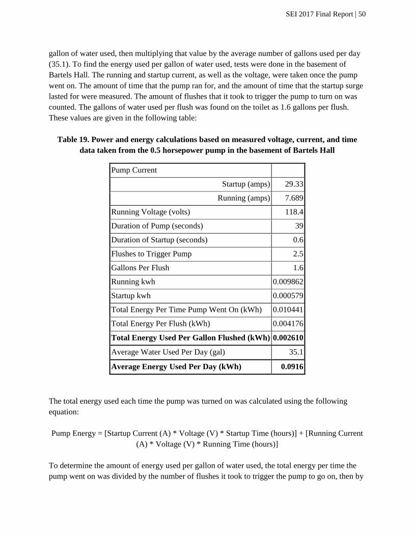
SEI 2017 Final Report | 50
gallon of water used, then multiplying that value by the average number of gallons used per day
(35.1). To find the energy used per gallon of water used, tests were done in the basement of
Bartels Hall. The running and startup current, as well as the voltage, were taken once the pump
went on. The amount of time that the pump ran for, and the amount of time that the startup surge
lasted for were measured. The amount of flushes that it took to trigger the pump to turn on was
counted. The gallons of water used per flush was found on the toilet as 1.6 gallons per flush.
These values are given in the following table:
Table 19. Power and energy calculations based on measured voltage, current, and time
data taken from the 0.5 horsepower pump in the basement of Bartels Hall
Pump Current
Startup (amps) 29.33
Running (amps) 7.689
Running Voltage (volts) 118.4
Duration of Pump (seconds) 39
Duration of Startup (seconds) 0.6
Flushes to Trigger Pump 2.5
Gallons Per Flush 1.6
Running kwh 0.009862
Startup kwh 0.000579
Total Energy Per Time Pump Went On (kWh) 0.010441
Total Energy Per Flush (kWh) 0.004176
Total Energy Used Per Gallon Flushed (kWh) 0.002610
Average Water Used Per Day (gal) 35.1
Average Energy Used Per Day (kWh) 0.0916
The total energy used each time the pump was turned on was calculated using the following
equation:
Pump Energy = [Startup Current (A) * Voltage (V) * Startup Time (hours)] + [Running Current
(A) * Voltage (V) * Running Time (hours)]
To determine the amount of energy used per gallon of water used, the total energy per time the
pump went on was divided by the number of flushes it took to trigger the pump to go on, then by

SEI 2017 Final Report | 51
the amount of gallons per flush. This gave a value of 0.002610 kWh used by the Bartels pump
per gallon of water used in the building. This was then multiplied by the average amount of
water that is used each day at that building to get the average amount of energy used by the
pump per day, which was 0.0916 kWh.
This was then compared to the amount of energy consumed per gallon of water going through
the well pump and the cistern pump. To get this value, the daily energy values for each of these
pumps was obtained from records kept near the pumps, and these were averaged to get an
average daily energy use of each pump (0.920 kWh for the well pump, 0.798 kWh for the cistern
pump). The amount of water used per day is also recorded at SML, so that too was averaged over
the course of the study to determine an average amount of water used per day (829.6 gallons).
The average energy of each pump was divided by the average water used by the island to
determine how much energy is required of each pump to pump one gallon of water (0.001122
kWh/gallon for the well pump, 0.0009989 kWh/gallon for the cistern pump). The average daily
water used at Bartels Hall was then multiplied by the amount of energy each pump required per
gallon of water to determine how much energy would have been used by each pump if the water
that supplied Bartels Hall was coming from the well. These two values (for the well pump, and
for the cistern pump) were then added together to get the total daily energy that would have been
used for the well and cistern pumps. The results of these calculations are summarized in Table
20.
Table 20. Well and cistern pump energy required to pump average daily water usage of
Bartels Hall
Average
Daily Energy
(kWh)
Average
Water Usage
(gal/day)
Average Energy
Used per Gallon
(kWh/gal)
Average Daily
Water Used at
Bartels (gal)
Equivalent Daily
Pump Energy
Used (kWh)
Well
Pump 0.920 829.6 0.001122 35.1 0.03939
Cistern
Pump 0.798 829.6 0.000989 35.1 0.03471
Total 0.07410
It would require 0.07410 kWh to pump the average daily water from the well and cistern pumps
to the pressure tanks. This value was compared to the amount that it would require to pump the
water using the pump in Bartels, which was 0.0916 kWh. This means that the pump in Bartels
Hall requires more energy per day to pump the water than the well and cistern pumps would to
pump the same amount of water. The difference was found between these, and it was used to

SEI 2017 Final Report | 52
calculate the extra money in diesel fuel that was needed per day, and per month, to power the
new pump. The results are summarized in Table 21.
Table 21. Energy and cost increase of pumping water from Bartels Hall basement cistern
compared to pumping from well with original pumping system
Average Daily
Energy Used at
Bartels Pump
(kWh)
Equivalent Daily
Cistern and Well
Pump Energy
Used (kWh)
Difference
(kWh)
Gallons of
Diesel per
kWh
Cost per
Gallon of
Diesel ($)
Daily
Increase in
Cost ($)
Monthly
Increase in
Cost ($)
0.0916 0.0741 0.0175 0.0903 2.2 0.0035 0.10
To determine how many gallons of diesel were used per kilowatt hour of energy consumed by
the island, the island’s diesel usage records were compared with the energy usage records. The
amount of diesel added to the generator per day was calculated by dividing the amount of diesel
added by the amount of energy used in the days that had gone by since diesel was added last. The
values were averaged to find the average gallons of diesel needed per kilowatt hour of energy
used by the island. Assuming a cost of diesel is $2.20 per gallon, which it was in the Portsmouth
area on the day that this calculation was done, the monthly increase in cost of the new Bartels
Hall pump was found using the following equation:
Monthly Increase in Energy Costs ($) = Daily Increase in Energy (kWh) * Gallons of Diesel
Used per kWh * Cost per Gallon of Diesel ($) * 30 days
This resulted in a monthly increase of cost of $0.10, and likewise a monthly increase in energy of
0.525 kWh. The amount of potable well water saved per month was also calculated by
multiplying the amount of gallons of rainwater used per day in Bartels Hall by 30, which yielded
1,053 gallons. These results are summarized below:
Table 22. Monthly water and energy changes resulting from new rooftop rainwater
collection, storage and distribution system in Bartels Hall
Bartels Rainwater Collection System Monthly Water and Energy Changes
Potable Well Water Saved (gallons) 1053
Energy Increase (kWh) 0.525
Cost Increase ($) $0.10

SEI 2017 Final Report | 53
The interns felt that the very slight increases in cost and energy use from the new system were
outweighed by the amount of water that was being pulled from the roof rather than the well.
The interns also considered possible improvements that could be made to this system. One
improvement that might be made is putting a force breaker, shown below, on the inflow pipe.
http://extension.psu.edu
Figure 9. Force breaker
The purpose of this force breaker is to absorb some of the energy of the water as it enters the
cistern. This prevents the incoming water from stirring up the settled particles, which can clog
the system if they are pulled into it. Similarly, the intake valve that brings water from the cistern
to the pressure tank could be lifted up a few feet from its current location at the base of the
cistern. This would prevent it from pulling settled particles that are on the bottom of the cistern
into the system. Although clogging of this piping system has not been an issue thus far, it could
potentially pose an issue in the future. If it becomes a large issue, an inline filter might be
necessary.

SEI 2017 Final Report | 54
Another recommendation that could make data collection and evaluating how well this system is
working easier would be to invest in a better way of measuring how much rain the island is
receiving, or moving the existing rain gauge to a less obstructed location. Several of the projects
that were completed this year required rain data from Portsmouth, NH, and may have been
slightly inaccurate as a result. Having more accurate rain data would allow SML to check for
leaks in the system, which was a concern.
The island should continue its regular maintenance of this system. Cleaning out the mesh filter is
of great importance, as a clogged filter can cause rainwater to leak out instead of going into the
cistern, as was observed in a rain event this month. In addition, this cistern should be emptied in
the winter off season so that it does not freeze and damage the cistern. After the water is emptied
from the cistern, the settled sediments on the bottom of the cistern can be cleaned out. Lastly,
SML might want to consider putting a cover on the cistern to keep it protected.
4.5.2 Water Use, Collection, and Storage
A toilet survey, shown below, was distributed to each bathroom in Bartels Hall and Founder’s
Hall. These surveys were conducted from June 23rd to July 7th, 2017.
Figure 10. Toilet survey that was distributed in Bartels Hall and Founder’s Hall from June
23rd to July 7th, 2017

SEI 2017 Final Report | 55
Over the course of the survey, an average of 8.9 people were staying in Bartels Hall on any given
day. The survey indicated an average of 5.7 flushes per day in the building. Given that each flush
uses 1.6 gallons of water, an average of 9.4 gallons of water should have been used each day.
However, the meter reading indicated that an average of 35.1 gallons were used per day. This
means that there was 3.7 times as much water used in Bartels as the surveys indicated. Applying
this error to the surveys in Founder’s Hall would yield a water usage of about 75 gallons per day,
as the survey indicated a water usage of about 20.2 gallons per day. The estimate may not have
been accurate due to the fact that the Founder’s Hall survey seemed to be more complete, so an
alternate method was used to determine the water usage in Founder’s Hall.
The average amount of water that each person used per day in Bartels Hall was calculated by
dividing the average daily water usage (35.1 gallons) by the average amount of people that were
staying there per day (8.9). This gave a value of 3.96 gallons per person per day. This was then
multiplied by the average amount of people who were staying in Founder’s Hall each day over
the course of the survey (13.2). This yielded an average daily water usage value of 52.2 gallons
per day in Founder’s Hall. This estimate was considerably less than the survey-based estimate of
75 gallons per day, which seemed very high. The current estimate was also most likely a liberal
estimate, as the residents of Bartels Hall were told to flush the toilet more prior to the survey, as
there was plenty of water in the cistern, and the island engineers wanted to see how well the
system responded to an increased demand. A summary of these calculations is shown below:
Survey Data:
Table 23. Calculated average gallons of water used per day in Bartels Hall and Founder’s
Hall based on survey data
Average
flushes per
day
Average
people per
day
Average flushes
per person per
day
Average gallons
of water per
person per day
Average
gallons used
per day
Bartels 5.733333333 8.866666667 0.6594011544 1.055041847 9.354704377
Founder's 12.6 13.2 0.9533177641 1.525308423 20.16

SEI 2017 Final Report | 56
Meter Data:
Table 24. Calculated average gallons of water used per day in Bartels Hall and Founder’s
Hall based on Bartels Hall water meter data. This data was deemed to be more accurate
than the data from table e, and thus was used in further calculations
Actual
average
gallons used
per day
Actual Average
gallons of water
use per person
per day
Safety
Factor
Safety Factor
Applied Average
Gallons Used per
Day
Average gallons of
water used per
day (using Bartels
meter)
Bartels 35.06875 3.95512218 3.74878228 35.06875
Founder's 75.57545076 52.20761278
Given this data, about 1,566 gallons of water would be needed each month. The cistern in Bartels
Hall regularly has about enough water on-demand to meet the monthly needs of the hall, so this
was used as a metric to determine if Founder’s Hall would receive enough water from rainfall.
This means that the roof should be able to collect about 1,600 gallons of water each month.
The eastern facing side of the roof was designated as the collection area for Founder’s Hall. The
length and width measurements of the roof were taken from the ground. For the ease of the
calculations, the doghouse dormer on the roof was not taken into consideration. The length of the
roof was determined to be 42.0 feet long. The width of the portion that was used was found to be
17.0 feet. However, the width of the actual rooftop area was slightly different, as it was on a
33.7˚ slope. The actual width was calculated as 20.4 feet considering the angle. The width and
length were multiplied together to get the area of the roof, which was 858 square feet. A diagram
of this roof is shown below:

SEI 2017 Final Report | 57
Figure 11. Rooftop measurements for Founder’s Hall. Note that the area highlighted in
yellow is the designated collection area
This means that if one inch of rain were to hit this section of the roof, 534.8 gallons of water
could be collected. This was calculated using the following equation:
Collected water = Rooftop area * 1 inch of water * (1 foot / 12 inches) * (7.48 gallons / 1 cubic
foot)
534.8 gallons = 858 ft^2 * 1 inch of water * (1 foot / 12 inches) * (7.48 gallons / 1 cubic foot)
The historical rainfall data for Portsmouth, NH was then considered to determine how much rain
could actually be expected in a given month. The rainfall data for the months of May through
August for the past ten years was considered. This data gave a monthly average of 3.108 inches
for May, 4.646 inches for June,4.239 inches for July, and 3.427 inches for August. All of these
average values would be able to collect more rainwater than the suggested monthly collection of
1,600 gallons. The lowest amount of precipitation recorded for each month was also considered
for the past ten years to mimic a worst-case scenario where there was an extremely dry summer.

SEI 2017 Final Report | 58
These values were 1.06 inches for May, 2.09 inches for June, 1.28 inches for July, and 1.20
inches for August. None of these values would provide enough water to support the needs of the
building if there were an extremely dry summer. It is recommended that the flushing water
distribution system for this building remain able to be switched over to the potable water supply
in the case of a dry summer. These values are summarized in Table 25.
Table 25. Amount of rooftop rainwater available per month for May through August given
an average summer and an absolute low summer
The next thing that the interns looked at for this project was where to store the water. Two
options were considered: placing storage tanks on an inclined concrete slab in the basement of
Founder’s Hall, or repairing the existing cistern that is in the basement. The available storage for
the tanks on the concrete slab is limited by how many tanks can fit on the slab, as well as how
the size of the tanks that can fit through the door into the basement. It was determined that three
tanks can fit on the slab with a total volume of 650 gallons. The usable volume of the cistern is
about 2100 gallons. Due to the fact that it was decided that 1600 gallons of water should be
available at all times, using the existing cistern to store the rainwater is recommended. Images of
the basement of Founder’s Hall (Figure 12), the existing cistern (Figure 13), and of the proposed
options for storing the water (Figures 14 and 15) are shown below.

SEI 2017 Final Report | 59
Figure 12. Picture of the basement of Founder’s Hall. To the right of the pole is the
concrete slab that could hold water storage tanks
Figure 13. Picture of the existing cistern in the basement of Founder’s Hall
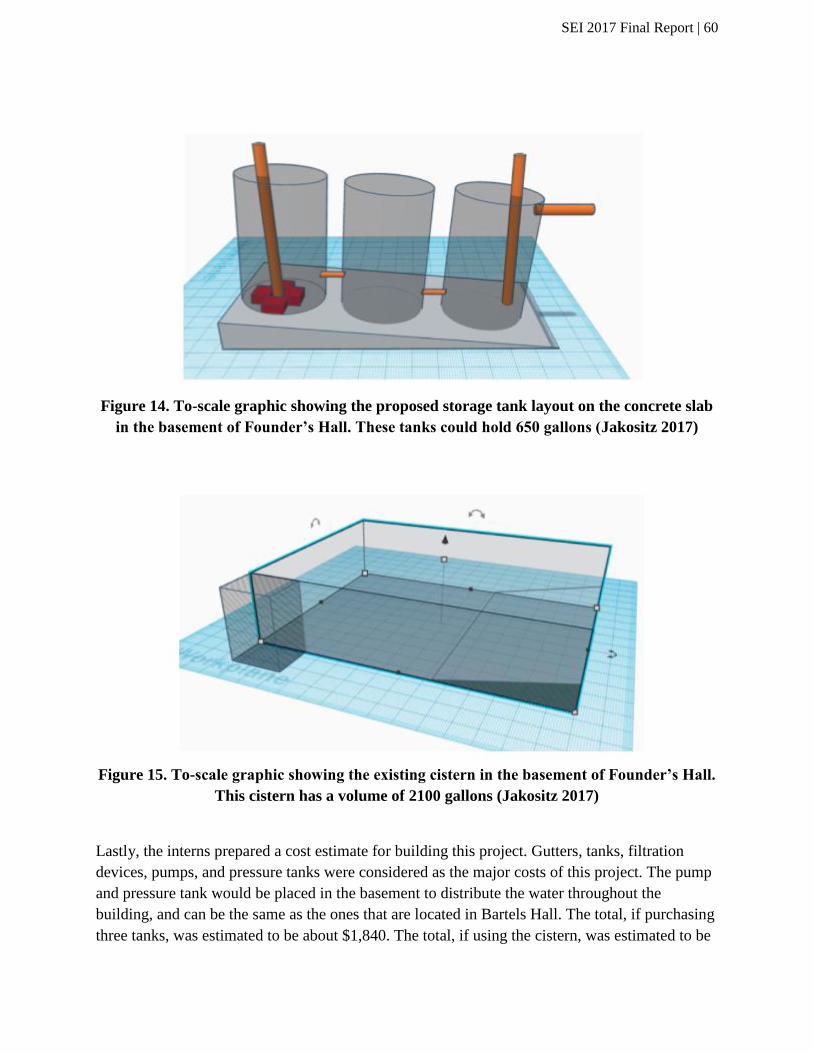
SEI 2017 Final Report | 60
Figure 14. To-scale graphic showing the proposed storage tank layout on the concrete slab
in the basement of Founder’s Hall. These tanks could hold 650 gallons (Jakositz 2017)
Figure 15. To-scale graphic showing the existing cistern in the basement of Founder’s Hall.
This cistern has a volume of 2100 gallons (Jakositz 2017)
Lastly, the interns prepared a cost estimate for building this project. Gutters, tanks, filtration
devices, pumps, and pressure tanks were considered as the major costs of this project. The pump
and pressure tank would be placed in the basement to distribute the water throughout the
building, and can be the same as the ones that are located in Bartels Hall. The total, if purchasing
three tanks, was estimated to be about $1,840. The total, if using the cistern, was estimated to be

SEI 2017 Final Report | 61
$1,050 before considering the costs related to repairing the cistern. Tables summarizing the costs
are given below:
Table 26. Summary of the capital costs of building the new rooftop rainwater collection,
storage, and distribution system for Founder’s Hall
In addition, the monthly cost of diesel fuel to power the pump was calculated. This was done by
assuming that the pump would use about the same amount of energy per flush as the one in
Bartels Hall would, about 0.0042 kWh per flush. Given the estimate of monthly water use in
Founder’s Hall to be 1,566 gallons, about 4 kWh of energy would be required to power this
pump each month. Given the previous calculations about how many gallons of diesel need to be
used per kWh of energy that the island uses and the assumption that diesel costs $2.20 per

SEI 2017 Final Report | 62
gallon, it would cost about $0.81 to power this pump each month. The results of this calculation
are summarized below:
Table 27. Summary of the monthly energy usage and cost to pump water from the
basement of Founder’s Hall to the rest of the building
4.6 Conclusions and Recommendations
The existing rooftop rainwater collection, storage, and distribution system in Bartels Hall is
working as expected. It is supplying the need for the building, and no major issues have been
observed. SML may want to try to limit the amount of sediment that can get into the system and
clog it by installing force breakers, lifting the intake valve, and installing an inline filter if
necessary. They may also want to consider a better way of measuring and recording how much
rain falls on Appledore each day.
The proposed rooftop rainwater collection system would be located on the eastern facing roof of
Founder’s Hall. In an average summer, there should be more than enough rain to meet the needs
of this hall, which should be slightly higher than those of Bartels Hall due to the increased
number of people who typically reside there at any given time. The proposed storage location of
this water would be in the existing 2100 gallon cistern in the basement of this building. Repairs
would need to be made before this cistern can be used, but it already has a hole in the wall, about
three feet up from the ground outside, where inflow pipes from the roof can enter the cistern.
This could also be a good spot for an overflow drain should there be too much water.
It is recommended that rainwater collection for this system begins as soon as someone comes out
to Appledore Island for the season, prior to May when it starts to get busier. That would allow
some accumulation of rainwater in the cistern prior to heavy usage. It would be particularly
advantageous to begin collection in a typically rainy month, such as July. If it is found that this
system is not collecting enough of the rainwater, the collection area can be expanded to include
the rest of the roof, or other rooftops nearby. There are plenty of unused roofs on the island that
are capable of collecting water. It is also recommended to keep the equipment in place to connect

SEI 2017 Final Report | 63
this system to the potable water supply as a backup so that it would be easy to switch back over
if there was not enough rainwater collection.
Implementing this system would reduce the load on the island’s potable water supply well and
would utilize a freshwater resource that would be otherwise unused.
4.7 References
John Durant, Tufts University
Tom Johnson, Johns Hopkins Applied Physics Laboratory
Ross Hansen, Shoals Marine Lab

SEI 2017 Final Report | 64
Assignment 5: Lifespan Analysis of the Green Grid Batteries
Project Leads: Leah Balkin and Eesha Khanna
5.1 Background
In 2014 SML installed a 300 kWh battery bank consisting of 40 absorbed glass mat (AGM)
batteries in green energy infrastructure improvements aimed at decreasing the generator running
time on the island. Like for any new system, there was a learning curve in identifying the most
efficient operational set points for the system. Batteries are the weak link in the energy system
and they will need to be replaced first. By analyzing data over the past three years, SML wishes
to make informed decisions about battery lifespan. SML feels that since it uses the batteries only
for 5 months every year, the batteries should last longer than the projected lifespan based on all
year use. The batteries are a very expensive part of any renewable energy system, and having this
information will be useful for long-term battery replacement planning purposes.
5.2 Purpose
SML wants a timeline to predict the lifespan of the current green grid batteries in order to know
when they have to seriously consider replacing the batteries.
5.3 Scope
Batteries have a limited lifespan and at some point they will need to be replaced. This is very
costly as the current batteries cost the island $100,000. A battery lifespan is determined by the
number of cycles that the battery runs through. A cycle is the charge and discharge of a battery.
Information on battery cycles is collected in the Energy Conservation Building in the form of
data on voltage, current, and the battery monitor. In addition, the lifespan of a battery is affected
by the depth of discharge, the level to which batteries are drawn down to before they are charged
again. The greater the depth of discharge, the shorter the lifespan.
5.4 Methods
5.4.1 Cycle Count
A battery lifespan is determined by the number of times it charges and discharges, or the number
of times it cycles. The interns also contacted the battery supplier, Absolyte, in order to get their
perspective on what counts as a battery cycle. According the Absolyte, a cycle is any time the
batteries drop in voltage and recharges afterwards.
Data has been collecting for the battery bank in the Energy Conservation Building for the voltage
and current levels every minute since their installation in 2014. The interns downloaded this data

SEI 2017 Final Report | 65
from the server and graphed the data for every day of the summer season that the batteries have
been running until the present. For the 2014 season and the first half of the 2015 season the
interns looked at the daily voltage cycles of the batteries. In July of 2015 SML installed a battery
monitor which offered a more reliable way to tell how many cycles the batteries had undergone.
From this time until the present the interns graphed the battery monitor voltage data for every
day and counted the number of cycles on each graph.
Many of the graphs were variable so the interns devised a system for determining what a cycle is.
Below is a typical example of one full battery cycle. The cycle begins at the orange arrow where
the batteries begin to charge and ends at the green arrow where the batteries have discharged to
their lowest voltage before they begin the cycle again.
Figure 16. Graphical depiction of a cycle, V
There are many spikes that can be found in this graph that occur over such a short period of time
that they do not count as a cycle. These account for times where the load on the battery bank
greatly increased for a short period of time because a new load was turned on. This occurs
because loads on the island such as the saltwater pump require a large starting voltage in order to
start running.

SEI 2017 Final Report | 66
In 2016 battery capacity data began to record which reveals a smoother trend for each cycle than
graphs for voltage. Below is the graph that aligns with the date of the voltage data in the graph
above. The same arrows are used to denote the beginning and end of one cycle.
Figure 17. Graphical depiction of a cycle, Ah
In this graph, the cycle is very evident since the sharp drops in from added loads that do not
affect the cycle count are not present. Therefore, the battery capacity graphs were used to check
the interns’ method for counting cycles.
In addition, the battery monitor data allowed the interns to calculate the depth of discharge. In
order to expand the lifespan of a battery it is not discharged fully before it recharges. The lowest
voltage that a battery is programmed to reach is called its depth of discharge. SML currently runs
their batteries with an average depth of discharge of 30% (battery only discharges to 70% before
it is recharged to 100%). The depth of discharge is most accurately calculated using battery
monitor data on battery capacity. Since battery monitor data was only available after July 2015
and battery capacity was monitored starting in 2016, the interns assumed that before this time the
average depth of discharge was similar to the values it has been afterward.

SEI 2017 Final Report | 67
By analyzing the number of cycles that the batteries had undergone since their installation and
the available data on the depth of discharge, the interns estimated the approximate lifespan the
batteries have remaining.
The following graph shows the cycles of a battery over the course of four weeks. The interns
analyzed the day-to-day graphs to get a more in-depth view of each of these days.
Figure 18. Cycles of a battery over the course of four weeks
5.4.2 Research on Battery Maintenance
There are many factors that affect the lifespan of batteries. These include temperature and
conditions in which the batteries live, how they are charged, the condition they are left in when
not being used, etc. The interns researched all of these factors in order to understand how the
batteries should be operated and maintained. Lee Consavage, Alex Brickett, the internet and the
instructions manual for Absolyte GP Batteries were consulted to facilitate this research.
5.5 Results and Analysis
5.5.1 Cycle Count
While analyzing the graphs, the interns ran into several different complications. Several (almost
all) graphs had sudden, momentary drops in voltage due to a heavy load being suddenly applied
(for instance, turning on a heavy appliance) and the interns did not account for these as separate
cycles as they lasted for a very short period of time (~2 minutes or less). Many graphs had
sudden spikes in voltage and these occurred when the system switched from PV/wind power to
generator power. These were also momentary and therefore, they were not accounted for as
separate cycles.

SEI 2017 Final Report | 68
Figure 19. Depiction of sudden spikes and drops in voltage
On certain days, there was incomplete charging of batteries, i.e. the batteries would start
discharging before being completely charged. It was found that this was the case on cloudy days,
when there was not enough solar power at certain times to handle the entire load, and therefore,
the batteries needed to be discharged during the day. The interns consulted Lee Consavage for
additional information and found that the last part of the charging (in the absorption stage)
requires extra power. Therefore, when the generator is handling the load in the day, the inverter
prevents the batteries from being charged fully. This is especially common on cloudy days when
there is not enough solar power to charge the batteries. Additionally, when the batteries do not go
over a 95% state of charge, there might be a voltage drop. The battery manufacturer was
consulted regarding this and it was found that low voltage is the natural state that the batteries
like to be in and therefore, nothing can be done to prevent this from happening. Based on what
the representative from GNB industries said, the interns decided to count these incomplete
charge cycles as full cycles.

SEI 2017 Final Report | 69
Figure 20. Example of incomplete charging
On certain days, the interns noticed incomplete discharging of batteries, i.e. the batteries did not
go to the 30% depth of discharge before being charged again. Perhaps, this occurred on days
when the island load was low, mostly during the beginning of the seasons or at the end of the
season. The interns accounted for these as full cycles, which might be a factor that caused slight
overestimation of results.
On certain days, there was a mid-cycle drop to 0V, and that meant that the system had been shut
down. The interns counted this as the end of a cycle to be on the safe side, and also because
when the system would turn back on, a new cycle would start.
Figure 21. Example of a mid-cycle drop to 0V
In 2014, there were several days with multiple cycles. There were several factors that caused
multiple cycles per day. The initial set points were based on the manufacturer’s recommendation,
but it turned out that they were not optimal for the system. It took a lot of trial and error to figure

SEI 2017 Final Report | 70
out the optimum set points. Another obstacle was tuning the system to work well in all weather
conditions. A particular setting worked well for sunny day, but not for cloudy days and vice-
versa. It took some time to come up with an arrangement that was optimal in all weather
conditions. Additionally, there was no battery monitor in the first year, which means there was
no accurate way of knowing state of charge of the batteries. The lack of the battery monitor was
also reflected when the wind turbine would skew voltages and trick the system into believing
that the batteries were being charged even when they were not. All these factors posed a learning
curve for Shoals to understand the working of the battery bank. The interns counted all of these
as full cycles even if they were not as deep as 30% because there was no battery monitor
installed back then, which helps determine depth of discharge. Therefore, the interns were not
sure about what the depth of discharge was for these cycles and how it would affect lifespan of
the batteries. The worst case was considered, which might have led to slight overestimation of
cycle count.
The following graph shows a day with 10 cycles. The part before the first triangle is the last part
of the cycle that started on the previous day and was counted as the first cycle for this day. The
part after the last triangle is the first part of the cycle that was completed on the next day, and
was counted as the first cycle for the next day. The part between the seventh and eighth triangles
is counted as one cycle because the varying voltage is very momentary, which means that this
part does not qualify as multiple cycles. The same applies for the part between the eighth and
ninth triangles. The momentary drop was perhaps due to a large load being applied and therefore,
this part qualifies as one cycle even though it might look like two at first glance.
Figure 22. Example of multiple cycles in one day

SEI 2017 Final Report | 71
After analyzing graphs for voltage and battery capacity from 2014 to the present, the interns
found the following results:
Table 28. Results of graphical analysis for voltage and battery capacity
Year Cycle Count Average Cycles/Day Depth of Discharge
2014 358 3.544 NA
2015 216 1.479 NA
2016 217 1.446 28.96
2017 (till 6/26) 64 1.143 28.08
Total 885 1.903
Using the data from the above graph (Figure 20) in the Methods Section, the depth of discharge
was calculated as follows:
Table 29. Calculated depth of discharge for the batteries
Lowest Battery Capacity 496 Ah
Total Battery Capacity 700Ah
𝐷𝑒𝑝𝑡ℎ 𝑜𝑓 𝐷𝑖𝑠𝑐ℎ𝑎𝑟𝑔𝑒 =𝐿𝑜𝑤𝑒𝑠𝑡 𝐵𝑎𝑡𝑡𝑒𝑟𝑦 𝐶𝑎𝑝𝑎𝑐𝑖𝑡𝑦
𝑇𝑜𝑡𝑎𝑙 𝐵𝑎𝑡𝑡𝑒𝑟𝑦 𝐶𝑎𝑝𝑎𝑐𝑖𝑡𝑦= 496/700 ∗ 100 = 70.1%
As can be seen from the data in Table 28, the batteries have undergone approximately 885 cycles
up until June 26th of 2017 at about a 30% depth of discharge. The island engineers want the
battery cycle count to be approximately one per day. As of right now, however, the average
cycles per day is 1.9. The reasons for this high average are looked into in the next section of this
report.
In addition, the interns looked at how the depth of discharge affects the number of cycles a
battery will have in its lifespan. From the following graph supplied by the battery manufacturer,
the interns were able to evaluate this. The data point for a 30% depth of discharge is marked with
a red line.

SEI 2017 Final Report | 72
Figure 23. Figure provided by manufacturer depicting number of cycles vs. depth of
discharge
After analyzing this graph, the interns found that with a 30% depth of discharge the batteries will
have approximately 4,000 cycles. The interns created a chart to show the percent of the lifespan
that the batteries have used each year assuming that the batteries will go through approximately
4,000 cycles in their lifespan.
Table 30. Percent of lifespan used and remaining each year
Year % Lifespan Used Per Year % Lifespan Used % Lifespan Remaining
2014 8.95 8.95 91.05
2015 5.4 14.35 85.65
2016 5.425 19.775 80.225
2017 1.6 21.375 78.625

SEI 2017 Final Report | 73
In order to project the number of years the batteries have left based on the 30% depth of
discharge, the interns calculated that the batteries have 3,115 cycles remaining. Even though the
average cycle count per day is 1.9, based on current data the interns used a 1.5 cycles per day
average to project the number of years remaining. This is because the 1.9 average was clearly
affected by the high average for 2014. Shoals will not see such a high average again because the
settings have been optimized and the engineers are more familiar with the system. The average
for the rest of the years (2015-2017) is less than 1.5, but the interns felt that 1.5 is a safe estimate.
Table 31. Projected number of years left in battery lifespan
Number of days per season (safe estimate) 150
Number of cycles per day (safe estimate) 1.5
Number of Shoals Seasons 13.84
Based on this average and the number of cycles remaining, it was predicted that the batteries
have about 13.8 more Shoals seasons. 13.84 also includes part of 2017, therefore, 13 seasons is a
good estimate. The batteries are expected to last until 2030.
Another consideration that the interns looked at was how many years the batteries would last at a
deeper depth of discharge. By running the batteries at a deeper depth, Shoals could get more
energy storage out of the batteries and work toward the goal of running off 100% renewable
energy. In addition, Shoals could keep up with the changing battery technology by needing to
buy new batteries sooner. There are batteries currently on the market that are more efficient than
AGM batteries and could also help Shoals reach its goal of running off 100% renewable energy.
Below is a table of the number of years that the batteries could get out of each depth of
discharge.
Table 32. Years of battery life permitted by various depths of discharge
DOD (%) Total Cycles Cycles Remaining Years Remaining
30 4000 3115 13.84444444
40 3500 2615 11.62222222
50 2500 1615 7.177777778
60 2000 1115 4.955555556
70 1600 715 3.177777778
80 1200 315 1.4

SEI 2017 Final Report | 74
5.5.2 Research on Battery Maintenance
5.5.2.1 Temperature and Temperature Variation
After going through the battery manual, the interns found that the optimum temperature for the
batteries is 25℃ and that the life span projected by the manufacturer is based on this
temperature. The table below shows how battery life span is reduced due to increased
temperature.
Table 33. Reduction in battery lifespan due to various temperatures, provided by
manufacturer
Although increased temperature is not a huge issue on Appledore Island, the summers do tend to
get fairly warm. Additionally, the Energy Conservation Buildings is built in a way that it does
not have any ventilation. The interns worked around that area and noticed that it tends to get
warm and stuffy inside. On certain days, the garage door is not opened, and this further
contributes to heating up the building.
Additionally, the interns found that it is not just important to keep the overall ambient
temperature around 25℃, but it is also important to reduce temperature variations. Temperature
variations within the strings of the batteries can result in voltage differences and can eventually
compromise battery performance. It is important to keep temperature variations within 3℃.
5.5.2.2 Deep Discharge of Batteries
Analysis of the state of charge data led the interns to confirm that the average depth of discharge
is approximately 30%. However, there were certain days when the batteries discharged deeply.
The following graph is the state of charge graph for June 24, 2017. On this day, the state of
charge fell down to 42%. This drop in state of charge was caused by a glitch in the AGS
(automatic generator start), which is supposed to switch the load to the inverter when the state of
charge reaches 70%.

SEI 2017 Final Report | 75
Figure 24. Sample day in which the state of charge of the batteries fell to about 42%
The interns consulted Alex Brickett and found that glitches in the AGS are one reason behind
deep discharge of batteries. Another historical reason behind deep discharge (that was evident in
2014 graphs) is the setting in the Schneider inverters that used voltage and not state of charge to
determine when to switch the load to the generator. On days when the wind turbine is moving
very fast and supplying a high voltage, the system can get tricked into thinking that the batteries
are being charged, even if they are not. However, this setting was changed when the Battery
Monitor was installed in 2015, so the only current issue in this regard is glitch in the AGS.
5.5.2.3 Charging of Batteries and Float Voltage
The interns looked into how the batteries were being charged and found that the 3 stage method
was being used. Further research led to the conclusion that the 3 stage method of charging is
optimum for the current system because the batteries are generally isolated from load while
charging. The interns particularly researched float voltage and how it affects the batteries. Float
voltage is the voltage at which a battery is maintained after being fully charged. It was found that
float voltage has a direct effect on service life of the battery and that it can also be the cause of
thermal instability. A float voltage above the recommended value reduces service life.
From the battery manual, it was found that the ideal float voltage is between 53.5 V and 54.5 V
at 25℃. The float voltage varies with temperature and therefore, it needs to be monitored. The
interns used a float voltage table from the battery manual, which specified the ideal float voltage
at different temperatures. This table was designed based on one cell, so the interns multiplied the
values with 24 (number of cells per battery (6) x number of batteries per string (4)).

SEI 2017 Final Report | 76
Table 34. Ideal float voltage of battery system at various temperatures
Temp (degrees C) Ideal Float Voltage (V) Temp (degrees C) Float Voltage (V)
7 56.4 22 54.48
8 56.4 23 54.48
9 56.16 24 54.24
10 56.16 25 54
11 55.92 26 54
12 55.92 27 53.76
13 55.68 28 53.76
14 55.68 29 53.52
15 55.44 30 53.52
16 55.2 31 53.28
17 55.2 32 53.28
18 54.96 33 53.04
19 54.96 34 53.04
20 54.72 35 52.8
21 54.72 36 52.8
Though the difference between the optimal float voltages does not seem like much (only a
fraction of a V), the batteries are extremely sensitive to these changes and therefore, it is
important to monitor the float voltage.
5.5.2.4 Winter Maintenance
Lee Consavage was consulted to determine the effect on battery life when the batteries are left
unused every winter for 7-8 months. The interns found that the batteries are left in an equalizing
charge state, i.e. they are just being charged, but not being used. This does not have any negative
effects on battery lifespan. In fact, batteries prefer being in a state of complete charge and not
being used. Moreover, it was found that the cold temperatures do not negatively affect the

SEI 2017 Final Report | 77
batteries as long as they are charging and are not directly exposed to snow or rain. The fact that
they are charging throughout the winter also helps heat them up.
5.6 Conclusions and Recommendations
Using the data from cycle counts and depth of discharge, an approximate 17 year lifespan is
predicted for the batteries. This lifespan is predicted to end sometime around 2030. That is, if
Shoals continues to run the batteries at a 30% depth of discharge and every season continues to
have an average cycle count per day of 1.5. In order to get more storage out of the batteries and
keep up with the changing technology in the battery world, the interns recommend that Shoals
look further into the pros and cons of setting the batteries at a higher depth of discharge.
Since temperature is a major factor that affects battery lifespan, the interns recommend SML to
install an air conditioner in the ECB in order to regulate the temperature. An air conditioner with
a high SEER (Seasonal Energy Efficiency Ratio) rating and a temperature sensor will be ideal. A
high SEER rating will ensure a low power consumption and a temperature sensor will ensure that
the air conditioner is not running when the actual temperature is 25℃ or lower. The interns also
observed that the air conditioner will not be an extra load on the system, especially on sunny, hot
days, when it is needed most. This is because the solar arrays already produce more energy than
can be stored. Since all that excess energy would go to waste anyway, using it to power an air
conditioner will be an effective use of that energy. The 2016 SEI interns looked at effective
usage methods for excess energy and the current interns feel that this is a good starting point.
Float voltage is another variable that needs to be monitored and adjusted, however, the need for
that will be eliminated if temperature can be regulated. Since there is no automated way to adjust
float voltage and someone would have to continuously monitor and change it according to
temperature, the interns feel that addressing the issue of varying temperature will address this
problem too and is perhaps the better solution to both the problems.
To understand why the AGS still fails sometimes, the interns contacted an engineer from
Schneider Electronics, who told them that the settings would have to be checked. Unfortunately,
this trip for an engineer from Schneider could not be arranged during the term of the interns.
Therefore, the interns recommend that the island engineers monitor depth of discharge of the
batteries closely and if the deep discharge problem arises again, they should immediately have
the system checked.
5.7 References
Alex Brickett, UNH Facilities and Relief Island Engineer
GNB Absolyte Exide Technologies
Schneider Electric

SEI 2017 Final Report | 78
Assignment 6: Using Rooftop Water for Additional Showers
Project Leads: Adrian D’Orlando and Sarah Jakositz
6.1 Background
SML gets most of its freshwater from a 22.5-foot dug well that is recharged by the surrounding
aquifer when it rains. In order to conserve freshwater, residents are asked to take “Navy
showers” no more than twice per week. By taking advantage of other freshwater sources such as
rainwater, SML would be able to expand its available water and allow for additional showers.
The interns explored the prospect of an outdoor shower in terms of water treatment, greywater
discharge, location of the shower, feasibility of a gravity-fed system, and volume of rainwater
collection.
6.2 Purpose
The purpose of this assignment was to design an outdoor shower and showering system to
support additional showers for SML residents. The shower would be supplied by rooftop-
collected rainwater and utilize a gravity-fed piping system.
6.3 Scope
The interns were tasked with designing an outdoor shower and showering system that will
collect, store, and distribute rooftop rainwater via gravity. Attention must be paid to regulations
surrounding the installation and use of the shower as well as cleanliness and usability of rooftop
collected water.
6.4 Methods
6.4.1 Regulation Research
The interns conducted extensive research in order to investigate any regulations surrounding the
installation of an outdoor shower in a coastal environment. The main source of information came
from phone calls with the Maine Department of Environmental Protection. The interns were
informed that regulations vary by town, and the local plumbing inspector would need to come
out in order to assess the particular situation and determine whether or not a shower can be
installed. However, regardless of the specific regulations that Appledore may fall under in this
situation, the Environmental Specialist in the Bureau of Water Quality from the Eastern Maine
Regional office noted that the discharged water from the shower would need to be treated. For
SML’s situation, this would most likely mean sending the discharge to the septic tanks and leach
field. In addition, due to the proximity of any area the shower may be built to the ocean and other
natural resources, the island may need to apply for a permit.

SEI 2017 Final Report | 79
As for water quality requirements, a shower must provide clean, potable water. This means that
any water that is collected in order to service the shower must be treated to the same standards
that the island’s drinking water is treated to.
6.4.2 Selecting a Location
The interns consulted Dr. John Durant about the project and possible locations for the shower.
The team took into account the fact that the system would need to be downhill of potential
rooftop collection locations so as to support a gravity-fed design. In addition, this location would
be particularly useful to those who spend time in the water, such as snorkelers or the dive class.
An outdoor shower would allow these participants to rinse off the salty water without using up
one of their precious two showers per week. As a result of its locational benefits, the team
decided to look into the Dive Locker as a potential location (Figure 25).
Figure 25. Proposed location for the outdoor shower/rinsing station in red beside the Dive
Locker
6.4.3 Water Collection Calculations
In order to determine whether or not the demand of additional showers could be supported, the
interns needed to calculate how much water a rooftop system could collect. The rooftop of
Kiggins Commons was chosen as the best roof to collect off of due to its large rooftop area. In
order to calculate how much water could be collected, interns took dimensions of a designated
section of roof (shown in yellow in Figure 26) and utilized the pitch of the roof to calculate
specific angles and adjust the diagonal measurements accordingly. This area could be expanded
to include more of the roof, however the interns began calculations utilizing only this section as
an experimental area to see how much water it would produce. The area of the roof was then
converted to square inches and multiplied by one inch of rain to determine what volume of water

SEI 2017 Final Report | 80
would be collected during a one-inch rainfall event. The volume was then converted to gallons to
be used for further analysis.
Figure 26. Calculated dimensions and area of the proposed Kiggins Commons rooftop
collection area
Using historical rainfall data from the past ten years for the months of May through August, the
average precipitation per active season was calculated. Precipitation data from the Portsmouth,
New Hampshire weather station was used, as it was the closest recorded location. This, however,
may mean that the data is not entirely accurate as Appledore and Portsmouth often experience
different levels of precipitation during storms. The average rainfall for each month was used to
calculate the rainfall for an average summer while the lowest recorded rainfall for each month
was used to calculate the amount of precipitation in a worst-case dry summer. This value was
then used to calculate how much rainwater would be collected off of the designated section of
roof on Kiggins Commons each month which was then broken down to a number of three-gallon
showers that could be taken in a given dry or average month.

SEI 2017 Final Report | 81
6.4.4 Head Calculations
Once the location at the Dive Locker was decided upon, the interns needed to perform head
calculations in order to determine whether or not the system could be supported solely by
gravity. There were assumptions made when performing these calculations, which included a
one-inch pipe, worst-case elevations, no bend losses, no pipe expansions or contractions, 50˚F
water, and an open flow with zero pressure at the exit. The Bernoulli Equation was then used to
calculate the energy available at both locations, taking into account losses due to friction in
pipes, valves, and entrances. To confirm the calculations, interns consulted Melissa Gloekler,
one of Dr. Nancy Kinner’s graduate students.
6.5 Results and Analysis
6.5.1 Feasibility
Due to the restrictions on regulations, installing an outdoor shower would not be possible
without treating the water supply as well as the discharged water.
According to the head calculations, the Dive Locker location would support a gravity-fed
system. It was determined, given the assumptions made, that a flow of about 8.3 gallons per
minute would be possible at the Dive Locker. This is more than enough flow, and can be reduced
as needed by modifying the piping system.
6.5.2 Water Supply
Based on the calculated area of the selected section of the Kiggins Commons roof along with the
historic rainfall data that was obtained, the interns calculated how many additional three-gallon
showers could be supplied each month of the summer season. There are two numbers calculated
for each month, one for a worst-case dry month and another for an average month based on
historic data from the past ten years. The calculated additional showers per month can be seen in
Figure 27.

SEI 2017 Final Report | 82
a.
b.
Figure 27. Additional three-gallon showers provided by the proposed system for average
monthly rainfall (a.) and low monthly rainfall (b.)
6.5.3 Water Storage
In order to store the collected water, the interns suggest that SML purchase plastic storage tanks.
Two tanks, one for settling and one for additional storage and distribution, would support the
system. The two tanks should be connected so as to allow water to flow from one to the other.
The first tank should be conical in order to support the settling of particles out of the water. A
conical tank allows to easy drainage of settled particles from the bottom. The second storage tank
would also allow for some settling, but mainly would be used for distribution so as to not disturb
water in the first tank and disrupt the settling process. The first tank was selected to hold 200
gallons, and the second to hold 400 gallons, allowing a total of 600 gallons of water to be stored
at any given time. If this amount is deemed too low, a third tank may be connected for additional
storage.
6.5.4 Total Cost
If SML were to implement the proposed system, Table 35 provides the approximate cost of the
rooftop collection and storage system as well as the piping and valves used to transport the water

SEI 2017 Final Report | 83
from Kiggins Commons to the Dive Locker, Founder’s Hall, and the holding tanks for Celia
Thaxter’s Garden. This cost estimate assumes two storage tanks, one conical with a volume of
200 gallons and one cylindrical with a volume of 400 gallons, 70 feet of gutters, 760 of piping,
two valves, and one inline filter. Disinfection costs and equipment were not included in this
calculation.
Table 35. Approximate total equipment costs for the proposed system
Gutters
Tanks
Filtration
Piping and Valves
Totals:
6.6 Conclusions and Recommendations
Due to the locational constraints for a typical outdoor shower as well as strict regulations
concerning the treatment of greywater, the interns suggest either installing a rinsing station
instead of a full shower or considering supporting the existing shower system with rooftop

SEI 2017 Final Report | 84
collected water. By treating the system as a rinsing station, which also could be treated as an
additional hose, those exiting the ocean would still have a resource to rinse off however the
island might not have to abide by as strict regulations pertaining to the discharge. Regardless, it
is still suggested that SML consult the local plumbing inspector to be sure that any system
installed follows Appledore-specific regulations. If SML is still looking to add additional full
showers for residents, they might want to look into a system to treat the water and use it to
supply the showering system that is already in place. Or, similarly, consider piping the collected
water to be treated in the potable water treating system and act as a supplement to SML’s potable
water cistern.
If SML is interested in implementing the proposed rinsing station, they will need to develop a
system to treat the collected water. A first step would be to incorporate a settling basin into the
collection tanks so as to remove large particles. Conical settling tanks are easy to drain settled
particles from and could be used in conjunction with a larger distribution tank so as to separate
settled water from water that has just entered from the gutters.
As SML would like to stray away from more chlorination, one option for treatment might be
installing an inline UV disinfection system. These systems are designed to treat
microbiologically contaminated ground or surface waters and some can offer a four-log or
99.99% reduction in bacteria, virus, and protozoan cysts. They range in size and price based on
required flow and do not add chemicals in the water as chlorination would, which could
otherwise create disinfection by-products. The systems are installed directly in line with the
plumbing pipes.
Although allowing for an additional shower or rinse each week might provide more comfort for
students and staff, SML should consider that this is not necessarily a necessity but a luxury. The
two showers per week rule is part of the culture on Appledore, and residents of the island do not
need more. Consideration might perhaps be better focused on how rooftop water can supplement
the showering system already in place or other potable water needs that the island demands. This
may also be done by utilizing the collected water to support the proposed Founder’s Hall toilet
flushing project as well as provide additional water to supplement the watering of Celia
Thaxter’s Garden.
6.7 References
Melissa Gloekler
Michael Loughlin, Specialist in the Bureau of Water Quality, Maine Department of
Environmental Protection

SEI 2017 Final Report | 85
Assignment 7: New Grease Trap Effectiveness
Project Leads: Leah Balkin and Eesha Khanna
7.1 Background
In 2016 the Sustainable Engineering Interns evaluated the working of the old grease trap and
found that it was not removing all the grease and solids before the stream entered the piping that
leads to the septic system. This led to the waste from the grease trap filling up the septic tank and
clogging the pipes. This created problems for SML because the grease and solid waste require
the septic tanks to be pumped more often, which is a very expensive task (approximately
$14,000). Therefore, the 2016 interns recommended that SML install a new, larger grease trap
that would be better equipped to handle the volume of grease from the kitchen.
On May 1st of 2017 the new grease trap was installed. SML wished to evaluate the new system
in order to ensure that it is working as planned. In addition, a maintenance schedule was needed
to prevent grease and solids from flowing into the septic system.
7.2 Purpose
SML wants to decrease the pumping frequency of the septic tanks because it is a very expensive
task. The new grease trap will be evaluated based on its effectiveness in removing the grease and
solid waste from the kitchen wastewater. In order to ensure that this effectiveness is maintained,
a cleaning schedule must be created.
7.3 Scope
This project evaluates the island's new grease trap based on the parameters that were tested for
the old grease trap in 2016. The temperature gradient across the grease trap needed to be
measured in order to make sure the temperature difference between the influent and effluent was
large enough for the FOGs to separate and form a top layer, and for the solid wastes to settle at
the bottom. In addition, coring samples needed to be taken from the influent of the tank and
effluent from the pipes leaving the tank. The influent sample reveals the composition of the tank,
which shows relatively how thick the layer of grease is. The effluent sample reveals whether
grease and solids are in the grey water that is heading to the septic tank. In addition, a
maintenance schedule can be determined by taking into account the thickness of the grease layer
and the amount of people the kitchen has cooked for.
7.4 Methods
7.4.1 Temperature Gradient

SEI 2017 Final Report | 86
Grease traps work by separating fats, oils, and grease (FOG) and food solids from kitchen
wastewater. As wastewater cools, the FOGs harden and the food solids settle. FOGs become
lighter than water and float to the top of the grease trap. Therefore, a temperature gradient across
the grease trap is required to ensure proper separation of layers. Testing was performed by
comparing the temperature of the water entering the grease trap (102°F) to the temperature of the
water leaving (88.5°F). This 13.5 degree cooling process is sufficient for the FOGs to coagulate
and rise, allowing the water to pass through the system.
7.4.2 Coring Samples
The interns compared the following coring samples:
Sample 1. Sample from inside the interceptor for the old (2016) and new grease trap (2017). This
sample was used to assess how well the new grease trap was working in separating FOGs and
solids, and also to observe the relative thickness in substance layers. In 2016, the layers in the
sample were indistinguishable since a large amount of grease had accumulated in the interceptor
that the sampler was clogged. In the 2017 interceptor the grease can be seen separated out from
the grey water, just as it is supposed to be.
a. b.
Figure 28. 2016 interceptor coring sample (a.) and 2017 interceptor coring sample (b.)
After taking the coring sample from the grease trap, the interns waited for 75 seconds (the
retention time, i.e. the time that water/sample is held in the grease interceptor) for the
FOGs and solids to separate out. Retention time was calculated as follows:
Dimensions of the grease layer on June 27 = 2’7” x 2’9” x 6”
Volume of the grease layer = 3.575 ft3 = 26.7 gallons
Volume of the tank = 125 gallons
Retention time = V/Q = volume/flow rate = 125 G/100 GPM = 75 seconds

SEI 2017 Final Report | 87
Sample 2. Downstream sample from the pipe leaving the outlet for the old (2016) and new
grease trap (2017). This sample was used to assess how the water looks after going through the
interceptor and to check if any FOGs or solids are still present in the water going to the septic
tanks. The images below illustrate the coring samples of the effluent from the interceptor taken
from the outlet pipes after the sample has passed through the interceptor. By comparing the two
different cores from 2016 and 2017, it can be concluded that the new grease trap is doing a much
better job of separating grease and solids out. In 2016, a significant portion of the grease and
food particles pass through the outlet, which is seen floating on the top and sitting at the bottom.
The effluent from the 2017 interceptor looks like dirty dishwater without solids or grease, which
means that the FOGs and solids are effectively being separated inside the interceptor.
a. b.
Figure 29. 2017 coring sample of effluent (a.) and 2016 coring sample of effluent (b.)
7.4.3 Maintenance Schedule
Andre Cardoso, a project manager who works with dining halls and grease traps at the University
of New Hampshire, visited SML to assist the interns in testing the temperature and coring
samples of the grease trap in both 2016 and 2017. He thought that the new grease trap was
working very effectively compared to the one in 2016. The interns worked with Andre to
measure the height of the layer of grease. They put a stick in the interceptor and waited till the
stick reached the water-grease interface. They knew that the stick had reached the interface when
bubbles would form on the top of the grease layer. They measured this height and made cleaning
recommendations based on the manufacturer’s recommendations, which said that the grease trap
should definitely be cleaned when the grease layer is 25% of the volume of the trap.
The new grease trap had been installed on May 1st of 2017 and had not been cleaned before
Andre and the interns examined it. The interns collected data from the Island Coordinator to find
out the number of people the kitchen cooked for at every meal, and added the numbers for the

SEI 2017 Final Report | 88
1.5 month period (May 10 - June 27) to find how many people the kitchen had cooked for in that
period.
7.4.4 Disposal Options
The interns looked into the different options for disposal of the grease collected from the grease
trap. The three options found were burning the grease, trashing it, or paying a recycling facility
to take it. The interns looked further into the last option. Andre Cardoso put the interns in touch
with Todd Berry from Clean Harbors, a company whose services University of New Hampshire
uses for the disposal of grease in its dining halls. The interns were also put in touch with Marty
McCrone, who is the Hazardous Waste Manager at UNH. The interns were able to come up with
a disposal plan after speaking to Todd and Marty.
7.5 Analysis and Results
7.5.1 Temperature Gradient
Grease melts between 100˚𝐹 and 120˚𝐹. In the new grease trap the kitchen wastewater enters at
102˚𝐹 and leaves at 88.5˚𝐹. Therefore, the gradient is adequate for the grease to solidify. The
grease becomes lighter than water and floats to the top as a result of the difference between the
specific gravity of grease and water.
7.5.2 Coring Samples
The analysis of the coring sample was qualitative. The 2017 interceptor sample formed a clear
layer of FOGs at the top of the column within the retention time (75 seconds), implying that the
new grease trap is working well. The 2016 interceptor sample did not separate into 3 distinct
layers, perhaps because of the accumulation of a large amount of FOGs. Therefore, in order to
ensure effective separation of FOGs and solids and to prevent clogging within the interceptor,
regular cleaning is necessary.
After analyzing the 2017 downstream sample, the interns saw that there was no trace of FOGs or
solids in the sample. This observation further validated the effectiveness of the new grease trap.
The 2016 SEIs had recommended installing another grease trap in series, but after looking at the
downstream sample, it can be concluded that another grease trap is not required.
7.5.3 Maintenance Schedule
The interns measured the grease layer in the 2’ interceptor to be 6”. Using the manufacturer’s
recommendation that the grease trap should be cleaned when the grease layer is 1/4th the height
of the grease trap, the interns recommended that the grease trap be cleaned immediately. For
future reference, the interns recommend that the grease trap be cleaned when the volume of the
grease is approximately 25 gallons or the height of the grease layer is 6”. Since it is difficult to

SEI 2017 Final Report | 89
keep opening the grease trap and measuring the height of the grease layer, the interns came up
with two monitoring points:
● The amount of people the kitchen has cooked for: ~7000 people
● The period of time that has passed since the last cleaning: 1-1.5 months
The interns recommend that once one of these parameters is met, the grease trap should be
checked and then cleaned if the height of the grease layer is ~6”. The length of time that passed
between the installation and the time that Andre recommended cleaned was 1.5 months from
May 10 to June 27. It should also be noted that this time during most of the month of May traffic
was light due to because students had not arrived on the island yet. Therefore, the interns
recommend that the monitoring point used be 1 month during busy months and 1.5 months
during slow months. Additionally, based on the data given by the Island Coordinator, the interns
found that the number of people the kitchen had cooked for was 7009.
7.5.4 Disposal Options
The interns came up with 3 disposal options, the pros and cons of which are in the table below.
Table 36. Pros and cons of three disposal options
Option Pro Con
Burn Easy, Free Bad for Environment and People
Trash Easy, Free Transport, Adds to landfill, Possibility
of spill
Recycle Sustainable Costs Money, Transport
While collecting the grease throughout the season and burning it is easy to do and does not cost
any money, it can be harmful for the environment and for people around. The interns were not
able to find harmful effects of burning grease specifically, but they did look into effects of open
burning and found that harmful toxins like dioxin, carbon monoxide may be released. Collecting
the grease throughout the season and trashing it on the mainland is also easy to do and does not
cost money, but it does need to be transported and adds to the landfill on the mainland and is
therefore not a very sustainable option. Additionally, there is also a possibility of spill. Recycling
the grease is a sustainable option, but it will need to be transported and will cost money.

SEI 2017 Final Report | 90
The interns presented a proposal to Shoals for the recycling option, just in case Shoals wanted to
go ahead with that option. The cost would be $110/55 gallon drum and since Marty McCrone
from UNH offered to include the waste in UNH’s disposal run, Shoals would not have to pay
extra money to Clean Harbors for transportation. Shoals would just have to deliver the grease to
the UNH port or campus in Durham. Because the weight limit for transportation is 4,000lbs,
hauling a 55 gallon drum should not present an issue for SML staff. The total cost for Shoals
would be approximately $220 per season as each round of cleaning generates about 27 gallons of
grease and there should be 3-4 rounds of cleaning per season.
The interns also looked into another company called Food Grease Trappers, but they were
offering a higher price. The interns feel that if Shoals decides to go ahead with the recycling
option, Clean Harbors will be the best option because of the pricing and the fact that they are
associated with UNH and therefore Shoals would not have to pay for transportation.
The interns feel that Clean Harbors would be a really great way to keep the island sustainable by
recycling waste. However, due to the cost of the service and the time SML staff would have to
devote to transfer the grease to Durham, this option might not be feasible for SML.
7.6 Conclusions and Recommendations
After analyzing the temperature gradient and coring samples, the interns came to the conclusion
that the newly installed interceptor is working effectively. The 2016 interns recommended
installing a 2nd grease trap in series if needed. After analyzing the downstream sample and
finding no food or grease particles, it does not look like a second grease trap is necessary.
As for a maintenance schedule, the interns recommend that the tank be cleaned when the height
of the grease layer is six inches. The monitoring points recommended are 1-1.5 months in terms
of time, or 7000 people in terms of the number of people the kitchen cooked for.
For disposal, the interns provided 3 options. They left it up to Shoals to decide what the best
option is as they did not feel qualified to make a recommendation the involves deciding between
an expensive but sustainable option and a free but unsustainable option.
7.7 References
Andre Cardoso, UNH Project Manager
Todd Berry, Clean Harbors
Marty McCrone, UNH Hazardous Waste Manager

SEI 2017 Final Report | 91
Assignment 8: Assessment of SML Groundwater Supply Well
and Surrounding Point Wells
Project Leads: Adrian D’Orlando and Sarah Jakositz
8.1 Background
Freshwater is a valuable resource on Appledore as the island relies solely on a 22.5-foot main
supply well to supply its running water. During particularly dry seasons, SML has been forced to
use the Reverse Osmosis (RO) system to produce freshwater when the main well runs too low.
The RO system is very energy-intensive and dramatically increases the volume of diesel fuel
consumed on the island, and therefore SML attempts to avoid using it at all costs. In a search to
expand their freshwater resources, the 2016 Sustainable Engineering Interns worked with Emery
& Garrett Groundwater Investigations (EGGI) to analyze Appledore Island’s groundwater and
located a site for a potential new well that appeared to not be hydraulically connected to the
aquifer that the current main well pulls from. A six-foot monitoring well was installed at the
designated location, although its depth was limited by bedrock that was hit approximately 6.4
feet down. This year’s interns were tasked with determining whether or not this well site was
hydraulically connected to the current supply well aquifer as well as work with EGGI to acquire
further knowledge about SML’s groundwater resources.
8.2 Purpose
The purpose of this assignment was to utilize groundwater analysis techniques to gain a better
understanding of the main freshwater well and surrounding aquifer with a focus on the hydraulic
connectivity between the six-foot monitoring well and main supply well.
8.3 Scope
The interns worked with John Brooks and Mike O’Brien, associates from EGGI, to analyze
properties of Appledore’s freshwater aquifer. Using data acquired from Leveloggers, as well as
other groundwater assessment techniques, interns compared water level fluctuations and
properties in four wells: the Main well, an 18-inch test well, a six-foot test well, and the Grass
Lab well. Results from this study added to SML’s growing knowledge of their freshwater
system.
8.4 Methods
8.4.1 Data Acquisition
During EGGI’s visit to Appledore on June 26th, John Brooks and Mike O’Brien met with the
interns to discuss various groundwater concepts and analytical techniques. Topics concerning

SEI 2017 Final Report | 92
groundwater behavior and analysis techniques were discussed. Afterwards, the group went out to
the wells to begin collecting data.
One of the tools used for the analysis of the wells were Leveloggers (Figure 30). Leveloggers are
automatic devices used for recording water levels based on pressure measurements. They hang
by a string from the top of a well and are submerged in the water, taking measurements every ten
minutes, which is the interval the data was calibrated to. Depth of water is determined by total
pressure, which is a sum of water pressure plus atmospheric pressure. With the help of EGGI,
barometric data over the period of study was used to account for atmospheric pressure and
extract the data that solely resulted from water pressure so as to determine accurate
measurements of water level.
Figure 30. Levelogger that was used to read water level data in each of the wells
A Levelogger was installed in each of the four wells on the island: the main supply well; the six-
foot well; an 18-inch, monitoring well located near the supply well; and the Grass Lab Well. The
interns and EGGI extracted the Leveloggers and downloaded the data using a special reader that
is hooked up to the computer in the Energy Conservation Building. The 18-inch well is located
in an area that is regularly saturated with surface water, and as a result yielded water level
measurements that were neither reliable nor useful for this study. The main focus was on
comparing fluctuations in water levels at the six-foot and main supply well. If the two fluctuated
in similar patterns, they would likely be influenced by the same pumping and recharge events
and thus there would be evidence that they are probably connected to the same aquifer.
Unfortunately, the Leveloggers in the six-foot well and Grass Lab well were discovered to be
dead when they were pulled out and hooked up to the reader. This meant that the interns had no
historic data to analyze for the six-foot well. New Leveloggers were installed in the two locations
to begin acquiring data.

SEI 2017 Final Report | 93
Because of the lack of previous data, the interns planned a pump test with the help of island
engineers Bob Austin and Zach Charewicz. The objective of this test was to simulate an event in
which a large volume of water was removed from the Supply Well at once so as to produce a
drastic change in water level that would be observably reflected at connected wells. On July 3rd,
the island engineers shut off the well pump and began to allow the potable water cistern to lower
in volume. After four days without the well pump on, the water level in the cistern reached a
level in which the well pump needed to be turned back on so as to avoid draining it too far. The
well pump was turned back on July 7th and ran for six hours to refill the cistern. The interns
waited two days to allow the wells some time to recover from the event, and pulled the
Leveloggers from each well on July 9th to begin analyzing data.
In order to make the water levels in each of the wells comparable to each other, the interns
determined the elevations of each of the wells by surveying a profile across the area of interest
and adjusting values according to a geodetic control point located just outside the Grass Lab.
With the help of EGGI, the interns incorporated elevation data into the water level data in order
to convert it into water level above Mean Tide Level.
With the help of EGGI, the interns also performed two slug tests and two pump tests on the six-
foot well (Figure 31). The purpose of these tests was to determine if the well was connected to
the surrounding aquifer. The slug tests involved first measuring depth to water level at static
conditions, and then pouring a gallon of water into the well and measuring the depth to water
level over a period of time as the water drew down into the ground. The test stopped once the
water level approximately reached its original condition. This test was performed twice, once
with the PVC pipe around the well and once without it. The pump tests involved first recording
the water level at static conditions and then pumping water out of the well with a peristaltic
pump at a recorded discharge rate of 0.36 gallons per minute. The depth to water level in the well
was recorded with a hand level every 30 seconds and the test stopped once the water level
stabilized. The first test did not reveal much change in water level, and so sediment was pumped
out of the well and a new depth to water was taken before a second pump test was conducted.
The water level stopped changing for a period of time even though it was still a foot lower than
its earlier static condition, so the well was left to stabilize for about two hours and 45 minutes
before taking a final depth to water measurement.

SEI 2017 Final Report | 94
Figure 31. Set-up for the slug and pump tests at the six-foot well
The interns and EGGI also measured a temperature and conductivity profile of the main supply
well on June 27th when EGGI was on Appledore. The team attached a tape measure to the
Levelogger and lowered it down the well at a rate of approximately one foot per minute and
raised it at the same rate. Data from top to bottom of well and from bottom to top of well was
downloaded in order to conduct a temperature vs. depth profile. As for conductivity, the team
lowered tubing connected to a peristaltic pump into the well at two-foot intervals. The pump
pumped water through the tubing and into a container. An Oakton CON150 conductivity meter
was used to measure the conductivity of the water as it filled the container. Measurements
started at the surface and continued every two feet until the bottom of the well was reached, and
then a second profile was conducted from the bottom of the well to the top at the same rate.
8.4.2 Data Analysis
Once the water level was adjusted according to barometric pressure data and elevation above
Mean Tide Level, the changing water level elevations were graphed over time. Graphed data
from the six-foot well, 18-inch well, and Grass Lab wells were visually compared to the main
supply well. If the water levels in two wells appeared to fluctuate in a similar pattern, over the

SEI 2017 Final Report | 95
same period of time, they were deemed to be hydraulically connected. According to EGGI, this
was an appropriate assumption and method to categorize the relationship between each well and
the main supply well.
8.5 Results and Analysis
8.5.1 Main Supply Well vs. Six-Foot Well
Figure 32 shows the water elevation above mean tide level of the main well in purple and the six-
foot well. The small dips on each line represent pumping of the well into the cistern, which is
done about twice a day. The larger increases represent rain events that replenish the supply of the
well faster than groundwater infiltration does. The two lines have roughly the same shape, so this
would indicate that the pumping events that influence the water level in the main well are also
influencing the water level in the six-foot well.
Figure 32. Water levels measured in feet above the mean tide level of the main well and six-
foot well from June 15th, 2017 to July 10th, 2017
8.5.2 Main Supply Well vs. Six-Foot Well, Pump Test
As previously mentioned, the Levelogger data from the six-foot well was not able to be retrieved
prior to June 27th, so to ensure that the data that was collected on July 9th would provide clear
results, interns conducted a pump test. The well pump was shut off on July 3rd, which is just a
few days prior to what Figure 33 shows. This allowed the water level in the wells to flatten out.
The water level in the cistern, which holds the water that is pumped out, was allowed to drop in
this time to prepare for the increased pumping event. The pump was turned back on July 7th and
the water was pumped for six hours, which is this blue section of the graph. The main supply
well responded immediately to the pumping event, and the water level decreased sharply due to
the amount of water that was removed in those six hours. The six-foot well also responded
quickly to this pumping event, but was not as extreme due to the fact that it was about 150 feet
away from where the water was removed. Assuming this similar response resulted from

SEI 2017 Final Report | 96
connectivity between the main well and six-foot well, the lesser drawdown in the six-foot well
can be attributed to its distance from the source of pumping. Due to an effect called the cone of
depression, drawdown in the main well results in drawdown in areas of the aquifer surrounding
the well, the degree of which decreases with an increase in distance between the well and
observed location. In pink on the graph is the period of time after the pump test when the well
was allowed to recover the water that was removed and go back towards its natural state. Again,
both the main well and the six-foot well showed a similar trend of increase.
Figure 33. Water levels measure in feet above mean tide level of the main well and six-foot
well from June 5th, 2017 to July 10th, 2017
8.5.3 Main Supply Well vs. Grass Lab Well
Figure 34 shows the water elevation above mean sea level of the main well (in purple), and the
Grass Lab well, which is shown in green. There does not seem to be a correlation in this data, but
it is difficult to tell because of the lack of data. Like the six-foot well, the Levelogger in the
Grass Lab well was dead when it was first retrieved on June 27th and so the only recent data
logged was from June 27th on after a new Levelogger had been placed in the well.

SEI 2017 Final Report | 97
Figure 34. Water levels measured in feet above mean tide level of the main well and the
Grass Lab well from June 5th, 2017 to July 10th, 2017
8.5.3 Main Supply Well vs. Grass Lab Well, Pump Test
The interns also looked at the pump test data to try to get a better idea as to if the main well and
Grass Lab well are connected. The wells do not appear to be hydraulically connected because the
Grass Lab well does not appear to respond to the well pumping or pump shut off. It is possible
that the effects of these events are too minor to be seen by this method due to the distance
between the two wells, but given this data they are most likely not connected.

SEI 2017 Final Report | 98
a.
b.
Figure 35 a, b. Water levels measured in feet above mean tide level of the main well (a.) and
Grass Lab well (b.) from June 5th, 2017 to July 10th, 2017
8.5.4 Six-Foot Well Slug and Pump Test Analysis
The raw data from the slug and pump tests can be found in the Appendix. Given the
responsiveness of the well to both of the tests, there is evidence to support the fact that the well is
connected to the aquifer.
Specific capacity was also calculated from the raw pump test data using the equation, Capacity =
Flow/Drawdown. Capacity is a quantification of whether the well will provide adequate water

SEI 2017 Final Report | 99
supply while being drawn down, and can also be used to estimate the optimum depth for
installing a pump. Pump test 1 yielded a specific capacity of 1.59 ft2/min and pump test 2 yielded
a value of 0.032 ft2/min. Pump test 1 lasted 1.5 minutes and occurred before debris was pumped
out of the well, and pump test 2 occurred right after the well was cleared of debris and was left to
return to static condition for 2.75 hours. An ideal pump test should be long so that the rate of
change in drawdown is small, and therefore the second pump test is likely the more credible.
8.5.5 Main Well Temperature and Conductivity Profiles
Raw data from the temperature and conductivity profile measurements can be found in the
Appendix.
The temperature profiles (Figure 36) were very similar in pattern, showing more drastic
temperatures at deeper depths. The well got progressively colder deeper down the well, which
was expected.
Figure 36. Temperature profile of main well, taken once from the top to bottom of the well
(blue) and once from the bottom to the top of the well (red)
The conductivity profile (Figure 37) showed peculiar results, with relatively high conductivity at
the top of the water level, a decrease in conductivity over the first few feet of water, and then
another increase over depth. The conductivity was expected to have increased with depth; as
water with a higher conductivity should be denser it was odd to have a lens of more saline water
at the top of the well. The representatives from EGGI did not have an explanation for this,
however conductivity ranges from 5.5µS for deionized water to 5S for seawater so the changes
that were observed were relatively minor. The EGGI representatives were not concerned by this
odd pattern.

SEI 2017 Final Report | 100
Figure 37. Conductivity profile of the main well, taken once from the top to the bottom of
the well (blue), and once from the bottom to the top of the well (red)
8.5.6 Survey Data
A survey was conducted to determine the heights of the wells and the water in the wells relative
to mean tide level. The results of the survey are shown in Figure 38 and summarized in Table 37.
It should be noted that the ground elevation for the six-foot well might not be entirely accurate,
as there were many large rocks surrounding the well and it was difficult to tell where the ground
surface actually was.

SEI 2017 Final Report | 101
Figure 38. Survey measurements for each well on Appledore Island, June 27th, 2017
Table 37. Summary of the ground elevation and top of casing elevation compared to mean
tide level for each well on Appledore Island, June 27th, 2017
8.6 Conclusions and Recommendations
Prior to the survey that the interns did, the ground elevation compared to the tide level was
unknown, so the well was only pumped down to a level of 10 feet below the bottom of the well
in order to avoid saltwater intrusion. Saltwater intrusion is when salt water is pulled into the
freshwater supply, which would contaminate the whole well. Typically, any pumping above the

SEI 2017 Final Report | 102
mean tide level, shown as the dotted blue line in Figure 39, would be safe to pull out without risk
of intrusion. It was recommended to not pull from below five feet above the mean tide level,
though, to be safe. The survey that the interns conducted showed that the elevation of the well
was 28.7 feet above the MTL. The depth of the well is 22.5 feet, so that means that the bottom of
the well is 6.2 feet above the MTL, which is above the five feet that is recommended. This
means that the well can be completely emptied without risk of saltwater intrusion, which gives
SML an extra ten feet of freshwater.
Figure 39. Diagram of the main supply well location above the mean tide level. The
freshwater lens is also shown below the MTL line. Not that this is not to scale
Based on the data that that was collected and analyzed, it seems like Shoals Marine Lab will
have to continue its search for a new source of freshwater. This will be of particular importance
as the lab community grows and will hopefully increase their capacity in the future. The interns’
recommendation would be to either dig deeper near the six-foot well location, as there is
speculation that there is another pocket of water beneath the bedrock barrier, or to try to locate a
new area for a well, potentially near Crystal Lake.

SEI 2017 Final Report | 103
In addition, the elevation data show that SML is able to drawdown the main supply well further
than ten feet without risk of saltwater intrusion. However, the supply well does not always refill
completely over the course of the off-season, and therefore drawing the well down to lower
levels might mean less water available the following year.
8.7 References
Emery & Garrett Groundwater Investigations- John Brooks and Mike O’Brien

SEI 2017 Final Report | 104
Future Project Suggestions
Cost-Benefit Analysis on Depth of Discharge
From the findings in 2017, Shoals has options to increase the green grid battery capacity by
setting the batteries at a higher depth of discharge. A cost-benefit analysis should be performed
on the system to see if it is worth the strain on the batteries to discharge them further as there is a
tradeoff between battery life and depth of discharge. Additionally, the future interns can also
look at the advantages and disadvantages of using a greater depth of discharge and having to
replace the batteries sooner. With the battery technology developing and improving at a rapid
pace, replacing these batteries sooner might be a good option to consider.
Radar Tower and Research Battery Technology
The Radar Tower batteries are the oldest in the energy system at Shoals so they will be the first
to need replacement. Shoals should look into alternatives to the Radar Tower batteries, both in
terms of new battery technology and new ways to distribute the load on the island. Lithium
batteries should be considered because of their superior technology.
Supplementing Potable Water System with Rooftop Collected Rainwater
SML is constantly searching for ways to reduce the use of and supplement their freshwater
resources. This year, the interns attempted to design a system in which rooftop collected
rainwater would provide additional showers for residents of the island, but discovered that this
water would need to be treated as potable water if it were to be used for a legitimate shower.
Instead of treating rooftop water separately to allow for its usage, SML might want to consider
designing a system that directs the collected water to the existing treatment system that prepares
water from the main supply well. This could allow for better water conservation without
reconfiguring plumbing or designing new showering units.
Further Investigations into the Six-Foot Well Site
There is a possibility that the results from this year’s groundwater investigations were not
thorough enough to determine whether or not the new potential well site (six-foot well) is
hydraulically connected to the current supply well. This is a result of the bedrock that limits the
depth of the six-foot test well. Further investigations should be carried out in order to determine
if this year’s results were representative of the six-foot well’s local groundwater properties, or if
there could perhaps be a pocket of water beneath the bedrock that is not hydraulically connected.


![[Internship Report] folder... · Web view[Internship Report] [Internship Report] 3 [Internship Report] Prince Mohammed Bin Fahd University College of Computer Engineering and Science](https://img.pdfslide.us/doc/110x75/5adbc5e37f8b9add658e5f6e/internship-report-folderweb-viewinternship-report-internship-report-3-internship.jpg)


![[ This report is NOT for Public Discussion ] INTERNSHIP REPORT : …ensearch.org/.../uploads/2012/04/2004-Internship-Report.pdf · 2017. 1. 14. · Undergraduate Internship: You-Han](https://img.pdfslide.us/doc/110x75/611747fc4585bd6cf00b5257/-this-report-is-not-for-public-discussion-internship-report-2017-1-14.jpg)