SUSTAIN - A Framework for Placement of Best ManagementPractices in Urban Watersheds to Protect Water QualityREPORT

Office of Research and DevelopmentNational Risk Management Research Laboratory - Water Supply and Water Resources Division

EPA/600/R-09/095 | September 2009 | www.epa.gov/nrmrl

SUSTAIN— A Framework for Placement of Best Management Practices in

Urban Watersheds to Protect Water Quality

by

Leslie Shoemaker, Ph.D. John Riverson Jr.

Khalid Alvi Jenny X. Zhen, Ph.D., P.E.

Sabu Paul, Ph.D., P.E. Teresa Rafi

Tetra Tech, Inc. 10306 Eaton Place, Suite 340

Fairfax, VA 22030

In Support of

EPA Contract No. GS-10F-0268K

Project Officer Dr. Fu-hsiung (Dennis) Lai

Water Supply and Water Resources Division 2890 Woodbridge Avenue (MS-104)

Edison, NJ 08837

National Risk Management Research Laboratory Office of Research and Development

U.S. Environmental Protection Agency Cincinnati, OH 45268

ii

Disclaimer

The U.S. Environmental Protection Agency, through its Office of Research and Development, funded and managed, and collaborated in the research described herein. It has been subjected to the Agency’s peer and administrative review and has been approved for publication. Any opinions expressed in this report are those of the author(s) and do not necessarily reflect the views of the Agency; therefore, no official endorsement should be inferred. Any mention of trade names or commercial products does not constitute endorsement or recommendation for use.

iii

Foreword

The U.S. Environmental Protection Agency (EPA) is charged by Congress with protecting the nation’s land, air, and water resources. Under a mandate of national environmental laws, the Agency strives to formulate and implement actions leading to a compatible balance between human activities and the ability of natural systems to support and nurture life. To meet that mandate, EPA’s research program is providing data and technical support for solving environmental problems today and building a science knowledge base necessary to manage our ecological resources wisely, understand how pollutants affect our health, and prevent or reduce environmental risks in the future.

The National Risk Management Research Laboratory (NRMRL) is the Agency’s center for investigation of technological and management approaches for preventing and reducing risks from pollution that threaten human health and the environment. The focus of the laboratory’s research program is on methods and their cost-effectiveness for prevention and control of pollution to air, land, water, and subsurface resources; protection of water quality in public water systems; remediation of contaminated sites, sediments and groundwater; prevention and control of indoor air pollution; and restoration of ecosystems. NRMRL collaborates with both public and private sector partners to foster technologies that reduce the cost of compliance and to anticipate emerging problems. NRMRL’s research provides solutions to environmental problems by developing and promoting technologies that protect and improve the environment; advancing scientific and engineering information to support regulatory and policy decisions; and providing the technical support and information transfer to ensure implementation of environmental regulations and strategies at the national, state, and community levels.

This document has been produced as part of the laboratory’s strategic long-term research plan. EPA’s Office of Research and Development has made it available to help the user community and to link researchers with their clients.

Sally Gutierrez, Director National Risk Management Research Laboratory

iv

Abstract

Watershed and stormwater managers need modeling tools to evaluate alternative plans for water quality management and flow abatement techniques in urban and developing areas. A watershed-scale, decision-support framework that is based on cost optimization is needed to support government and local watershed planning agencies as they coordinate watershed-scale investments to achieve needed improvements in water quality.

The U.S. Environmental Protection Agency (EPA) has been working since 2003 to develop such a decision-support system. The resulting modeling framework is called the System for Urban Stormwater Treatment and Analysis INtegration (SUSTAIN). The development of SUSTAIN represents an intensive effort by EPA to create a tool for evaluating, selecting, and placing BMPs in an urban watershed on the basis of user-defined cost and effectiveness criteria. SUSTAIN provides a public domain tool capable of evaluating the optimal location, type, and cost of stormwater BMPs needed to meet water quality goals. It is a tool designed to provide critically needed support to watershed practitioners at all levels in developing stormwater management evaluations and cost optimizations to meet their existing program needs. Due to the complexity of the integrated framework for watershed analysis and planning, users are expected to have a practical understanding of watershed and BMP modeling processes, and calibration and validation techniques.

SUSTAIN incorporates the best available research that could be practically applied to decision making, including the tested algorithms from SWMM, HSPF, and other BMP modeling techniques. Linking those methods into a seamless system provides a balance between computational complexity and practical problem solving. The modular approach used in SUSTAIN facilitates updates as new solutions become available.

One major technical requirement for SUSTAIN is the ability to evaluate management practices at multiple scales, ranging from local to watershed applications. The local-scale evaluation involves simulations of individual BMPs and analyses of the impact of various combinations of practices and treatment trains on local water quantity and quality. The larger-scale evaluation could involve implementing hundreds or thousands of individual management practices to achieve a desired cumulative benefit. The required simulations and cost comparisons of such large-scale, distributed BMP options place significant challenges on the computational accuracy and simulation time for system modeling. SUSTAIN incorporates an innovative, tiered approach that allows for cost-effectiveness evaluation of both individual and multiple nested watersheds to address the needs of both local- and regional-scale applications.

Previously available modeling tools are significantly limited with respect to simulation of sediment generation and its fate through natural runoff and treatment at a BMP. SUSTAIN partially resolves these sediment routing issues by considering three sediment fractions (i.e., sand, silt, and clay), but this

approach remains a compromise because the state-of-the-art knowledge and the needed monitoring data are still limited.

The SUSTAIN framework provides a comprehensive system with a modular structure that facilitates the incorporation of improved technologies in optimization, BMP simulation, and computational efficiency. A flexible integration and implementation of these improved methods and algorithms will be the focus of further enhancements to SUSTAIN. Expanding the SUSTAIN capabilities will allow users to choose the level of complexity and simulation detail that best suits project needs. EPA intends to support expansion of the capabilities and functionalities of the system to meet continuing water quality goals and the needs of the user community.

This document describes the rationale for developing the framework and the uses of the framework; explains the system’s design, structure, and performance; details the underlying methods and algorithms that provide the framework’s predictive capabilities; and demonstrates the framework’s capabilities through two case studies.

v

vi

Table of Contents

Chapter 1 Introduction.........................................................................................................................1-1 1.1. Project Rationale .......................................................................................................................1-1 1.2. Overview of SUSTAIN ..............................................................................................................1-3

1.2.1. Structure of SUSTAIN ......................................................................................................1-3 1.2.2. Multiple Scale Application Features................................................................................1-6

1.3. The Role of SUSTAIN in Watershed Applications....................................................................1-7 1.3.1. TMDL Development and Implementation.......................................................................1-8 1.3.2. Evaluation of GI Practices as Part of a CSO Control Program........................................1-9

1.4. SUSTAIN Application Process ................................................................................................1-10 1.5. About this Report ....................................................................................................................1-13

Chapter 2 SUSTAIN Design and Structure ........................................................................................2-14 2.1. Framework Manager ...............................................................................................................2-14 2.2. Simulation Modules ................................................................................................................2-16 2.3. Optimization Module ..............................................................................................................2-20 2.4. Post-Processor .........................................................................................................................2-22 2.5. Summary .................................................................................................................................2-24

Chapter 3 Simulation Methods and Algorithms ................................................................................3-25 3.1. Framework Manager ...............................................................................................................3-27

3.1.1. Data Management Component ......................................................................................3-27 3.1.2. BMP Site Selection........................................................................................................3-28 3.1.3. Routing Network............................................................................................................3-30

3.2. Land Module ...........................................................................................................................3-31 3.2.1. Weather Component ......................................................................................................3-33 3.2.2. Hydrology Component ..................................................................................................3-35 3.2.3. Water Quality Component .............................................................................................3-41 3.2.4. Important Considerations and Limitations: Land Module.............................................3-47

3.3. BMP Module ...........................................................................................................................3-49 3.3.1. BMP Simulation Component.........................................................................................3-52 3.3.2. Overland Flow Routing and Pollutant Interception .......................................................3-59 3.3.3. Aggregate BMP Component..........................................................................................3-63 3.3.4. BMP Cost Database Component ...................................................................................3-65 3.3.5. Summary of Management Practices and Treatment Processes in SUSTAIN .................3-72 3.3.6. Important Considerations and Limitations of the BMP Module....................................3-72

3.4. Conveyance Module................................................................................................................3-74 3.4.1. Methodology..................................................................................................................3-74 3.4.2. Important Considerations and Limitations of the Conveyance Module ........................3-82

3.5. Optimization Module ..............................................................................................................3-83 3.5.1. Problem Formulation .....................................................................................................3-83 3.5.2. Optimization Algorithms ...............................................................................................3-86 3.5.3. Regional Application .....................................................................................................3-90 3.5.4. Important Considerations and Limitations: Optimization Module ...............................3-92

3.6. Post-Processor for Results Interpretation ................................................................................3-93 3.6.1. Storm Event Classification ............................................................................................3-93 3.6.2. Storm Event Viewer.......................................................................................................3-95 3.6.3. Storm Performance Summary........................................................................................3-97

3.6.4. Cost-effectiveness Curve .............................................................................................3-100 3.6.5. Important Considerations and Limitations: Post-Processor.........................................3-103

Chapter 4 Case Studies ....................................................................................................................4-104 4.1. Upper North Branch Oak Creek Watershed..........................................................................4-104

4.1.1. Project Setting..............................................................................................................4-105 4.1.2. Data Collection and Analysis.......................................................................................4-108 4.1.3. Project Setup ................................................................................................................4-108 4.1.4. Optimization and Results Analysis..............................................................................4-112 4.1.5. Summary......................................................................................................................4-120

4.2. Little Rocky Run Watershed .................................................................................................4-121 4.2.1. Project Setting..............................................................................................................4-121 4.2.2. Data Collection and Analysis.......................................................................................4-122 4.2.3. Project Setup ................................................................................................................4-122 4.2.4. Optimization and Results Analysis..............................................................................4-128 4.2.5. Summary......................................................................................................................4-137

Chapter 5 References .......................................................................................................................5-138

Appendices Appendix A. Needs Analysis and Technical Requirements .................................................................A-143 Appendix B. Model Evaluation and Selection ..................................................................................... B-151 Appendix C. Summary of the Optimization Technical Panel Meeting ................................................ C-177 Appendix D. Appendix References ......................................................................................................D-185

vii

viii

List of Figures Figure 1-1. Overview of SUSTAIN components........................................................................................1-4 Figure 1-2. Watershed assessment points. .................................................................................................1-5 Figure 1-3. Sample cost-effectiveness curve. ............................................................................................1-5 Figure 1-4. SUSTAIN’s multiple scales of application. .............................................................................1-6 Figure 1-5. Tiered application of SUSTAIN for developing cost-effectiveness curves. ............................1-7 Figure 1-6. Using SUSTAIN in the watershed planning process. ..............................................................1-8 Figure 1-7. SUSTAIN application process. ..............................................................................................1-10 Figure 2-1. SUSTAIN components and flow chart...................................................................................2-15 Figure 2-2. Comparison of runtime for various simulation units and periods.........................................2-19 Figure 2-3. Comparison of runtime for 1-yr simulation of various units. ...............................................2-19 Figure 2-4. Scatter Search evaluation scenario results. ...........................................................................2-21 Figure 2-5. NSGA-II evaluation scenario results. ...................................................................................2-21 Figure 2-6. Example storm event classification graph. ...........................................................................2-22 Figure 2-7. Example storm event viewer graph.......................................................................................2-23 Figure 2-8. Example performance summary report graph.......................................................................2-23 Figure 2-9. Example cost-effectiveness curve. ........................................................................................2-24 Figure 3-1. The routing network showing the connections among the simulation components. ...........3-30 Figure 3-2. Schematic showing the land simulation processes. ..............................................................3-31 Figure 3-3. Conceptual view of surface runoff........................................................................................3-37 Figure 3-4. Two-zone groundwater model adapted from SWMM..........................................................3-39 Figure 3-5. Two-zone soil moisture storage under low water table condition. .......................................3-40 Figure 3-6. Two-zone soil moisture storage under high water table conditions......................................3-41 Figure 3-7. Schematic of sediment production and removal processes...................................................3-42 Figure 3-8. A schematic showing the BMP simulation processes modeled in SUSTAIN. ......................3-49 Figure 3-9. Wetland/lake/reservoir weir and orifice outflow. .................................................................3-52 Figure 3-10. Processes considered in an underdrain structure.................................................................3-56 Figure 3-11. Conceptual pond shapes simulated by Persson et al. (1999). .............................................3-58 Figure 3-12. Filter description for the sediment transport algorithm.......................................................3-61 Figure 3-13. Generic aggregate BMP schematic. ....................................................................................3-64 Figure 3-14. Illustration of land use area assignment to aggregate BMP components............................3-64 Figure 3-15. Aggregate BMP testing configuration. ...............................................................................3-65 Figure 3-16. Schematic of sediment transport, deposition, and scour in conduits. .................................3-76 Figure 3-17. Conceptual overview of the optimization module. .............................................................3-84 Figure 3-18. Illustration of assessment points. ........................................................................................3-84 Figure 3-19. Comparison of Scatter Search and NSGA II optimization techniques. ..............................3-87 Figure 3-20. Tiered application of SUSTAIN for developing cost-effectiveness curves. ........................3-91 Figure 3-21. Construction of the tier-2 search domain using tier-1 results. ............................................3-91 Figure 3-22. Simulation process for each iteration run. ..........................................................................3-92 Figure 3-23. Number of storm events and total precipitation and peak intensity as a function of

dry hours between storms....................................................................................................3-94 Figure 3-24. Precipitation events sorted by total precipitation volume and peak intensity. ....................3-95 Figure 3-25. Storm event 1: August 9, 2001 6:00 p.m. to August 9, 2001 8:00 p.m. (0.66 in. to

2 wet hours, peak: 0.48 in.). ................................................................................................3-96 Figure 3-26. Storm event 2: May 14, 2001 11:00 a.m. to May 14, 2001 1:00 p.m. (0.95 in. to 4

wet hours, peak: 0.38 in.). ...................................................................................................3-96 Figure 3-27. Storm event 3: April 20, 2001 2:00 a.m. to April 21, 2001 5:00 a.m. (1.03 in. to 12

wet hours, peak: 0.30 in.). ...................................................................................................3-97

ix

Figure 3-28. Storm event 4: February 8, 2001 12:00 a.m. to February 9, 2001 4:00 p.m. (2.34 in. to 25 wet hours, peak: 0.61 in.)......................................................................................3-98

Figure 3-29. Sediment removal summary for 34 storm events arranged by baseline sediment load......................................................................................................................................3-98

Figure 3-30. Peak flow reduction summary for 34 storm events arranged by peak flows. ....................3-99 Figure 3-31. Peak flow comparison by storm event arranged by post-developed peak flows. ..............3-99 Figure 3-32. EMC of sediment for the corresponding storms. ..............................................................3-100 Figure 3-33. Example cost-effectiveness curve for sediment load reduction. .......................................3-100 Figure 3-34. BMP cost distribution by effectiveness for sediment load reduction on the cost-

effectiveness curve. ...........................................................................................................3-101 Figure 3-35. Example cost-effectiveness and cost-distribution pair......................................................3-102 Figure 3-36. BMP storage distribution by cost-effectiveness interval. .................................................3-103 Figure 4-1. Oak Creek Watershed and Upper North Branch Oak Creek...............................................4-106 Figure 4-2. Upper North Branch Oak Creek Watershed case study road map. .....................................4-108 Figure 4-3. Average annual precipitation volume at Milwaukee Airport for water years 1988–

2002...................................................................................................................................4-109 Figure 4-4. Rainfall volume and intensity wet-interval distribution for water year 2001. ....................4-109 Figure 4-5. Comparison of daily flow at Model Outlet 58 with USGS 04087204 at South

Milwaukee.........................................................................................................................4-110 Figure 4-6. Comparison of monthly flow at Model outlet 58 with USGS 04087204 at South

Milwaukee.........................................................................................................................4-110 Figure 4-7. Modeled vs. observed TSS (mg/L) at Oak Creek gage OC-05, water years 1995–

2001...................................................................................................................................4-111 Figure 4-8. Modeled vs. observed TSS (mg/L) at Oak Creek gage OC-05, water year 2001. ..............4-111 Figure 4-9. Land use distribution in the modeled subwatersheds..........................................................4-112 Figure 4-10. Subwatershed grouping for two-tiered optimization. .......................................................4-113 Figure 4-11. Aggregate BMP schematic. ..............................................................................................4-114 Figure 4-12. Aggregate BMP land use distribution...............................................................................4-114 Figure 4-13. Aggregate BMP arrangement in tier-1 subwatershed A. ..................................................4-116 Figure 4-14. Tier-1 cost-effectiveness curve for subwatershed A with the selected solutions..............4-117 Figure 4-15. Composition of best solutions on tier-1 cost-effectiveness curve for subwatershed

A........................................................................................................................................4-118 Figure 4-16. Schematic of tier-2 analysis network. ...............................................................................4-119 Figure 4-17. Tier-2 cost-effectiveness curve. ........................................................................................4-119 Figure 4-18. Little Rocky Run watershed in Fairfax County, Virginia. ................................................4-122 Figure 4-19. Selected study area in Little Rocky Run watershed..........................................................4-123 Figure 4-20. Little Rocky Run case study road map. ............................................................................4-123 Figure 4-21. SWMM calibration results at junction 3 of the Little Rocky Run watershed. ..................4-125 Figure 4-22. Representation of three subareas.......................................................................................4-126 Figure 4-23. SWMM-generated hydrograph at the outlet of the study area. .........................................4-127 Figure 4-24. SWMM versus SUSTAIN-generated hydrograph comparison..........................................4-127 Figure 4-25. BMP placement schematic in the Little Rocky Run case study area. ...............................4-131 Figure 4-26. Annual precipitation at the Washington Dulles International Airport. .............................4-134 Figure 4-27. Volume and intensity distribution of storm events in 1994. .............................................4-134 Figure 4-28. Results showing the benefits of BMPs. ............................................................................4-135 Figure 4-29. Domain of optimization searches and identified best solutions........................................4-136

List of Tables Table 1-1. Management Practices Supported by SUSTAIN.......................................................................1-4 Table 1-2. Typical Data Needs for SUSTAIN Application ......................................................................1-12 Table 2-1. Simulation of Sediment Transport in SUSTAIN.....................................................................2-17 Table 2-2. Transport Simulation of Other Pollutants in SUSTAIN ..........................................................2-18 Table 3-1. Modules and Components in SUSTAIN .................................................................................3-26 Table 3-2. Summary of Inputs, Methods, and Outputs in FM.................................................................3-27 Table 3-3. GIS Data Requirement for BMP Suitability Analysis............................................................3-28 Table 3-4. Default Criteria for BMP Suitable Locations Used in SUSTAIN ...........................................3-29 Table 3-5. Structural BMP Options Available in the BMP Siting Tool ..................................................3-30 Table 3-6. Inputs, Methods, and Outputs of the Land Module................................................................3-32 Table 3-7. Land Simulation Methods Used in SUSTAIN ........................................................................3-33 Table 3-8. Green-Ampt Parameters .........................................................................................................3-37 Table 3-9. List of Sediment Input Parameters for Pervious Land ...........................................................3-44 Table 3-10. Range of Values for Sediment Erosion Parameters for Pervious Land................................3-45 Table 3-11. Typical EMCs in Urban Runoff ...........................................................................................3-47 Table 3-12. Summary of Inputs, Methods, and Outputs in the BMP Module.........................................3-50 Table 3-13. Available Optional Methods for BMP Simulation Processes ..............................................3-50 Table 3-14. Representative BMPs and Recommended Simulation Methods ..........................................3-51 Table 3-15. Coefficient Cw (English units) for Rectangular Sharp-Crested Weirs.................................3-53 Table 3-16. Quality Ratings of Conceptual Pond Shapes Simulated by Persson et al. (1999)................3-58 Table 3-17. Recommended k' and C* Values..........................................................................................3-59 Table 3-18. Comparison of Aggregate vs. Distributed BMP Results......................................................3-66 Table 3-19. Simulation Run-Time Comparison: Aggregate vs. Distributed ...........................................3-66 Table 3-20. BMPs and Associated Construction Components................................................................3-67 Table 3-21. Components..........................................................................................................................3-70 Table 3-22. BMP Types...........................................................................................................................3-70 Table 3-23. BMP Components ................................................................................................................3-70 Table 3-24. Component Costs .................................................................................................................3-70 Table 3-25. Unit Types............................................................................................................................3-70 Table 3-26. Reference Sources ................................................................................................................3-71 Table 3-27. Structural BMPs and Major Treatment Processes................................................................3-73 Table 3-28. Summary of Inputs, Methods, and Outputs of the Conveyance Module .............................3-75 Table 3-29. Typical Manning’s Roughness Coefficient for Closed Pipes...............................................3-75 Table 3-30. Typical Manning’s Roughness Coefficient for Open Channels...........................................3-76 Table 3-31. List of Sediment Input Parameters for the Reach.................................................................3-82 Table 3-32. Summary of Inputs, Methods, and Outputs in the Optimization Module ............................3-83 Table 3-33. Example Control Targets for Typical Evaluation Factor Assessment in SUSTAIN.............3-85 Table 3-34. Post-processor Inputs, Methods, and Outputs ......................................................................3-94 Table 4-1. Watershed Characteristics ....................................................................................................4-106 Table 4-2. Upper North Branch Oak Creek Land Use Distribution ......................................................4-107 Table 4-3. Summary of Modeled Annual Average Outflow and TSS Load in Oak Creek

Watershed..........................................................................................................................4-111 Table 4-4. BMP Parameters...................................................................................................................4-115 Table 4-5. BMP Cost Functions for the Case Study..............................................................................4-116 Table 4-6. Selected Tier-1 Solutions on the Cost-Effectiveness Curve.................................................4-117 Table 4-7. Selected Tier-2 Best Solutions .............................................................................................4-120 Table 4-8. List of Input Parameters for Both the Anderson and the USGS Methods............................4-124

x

xi

Table 4-9. Comparison of Predicted Peak Flows (ft3/s) in the Little Rocky Run Watershed................4-125 Table 4-10. Land Uses of the Case Study Area in the Little Rocky Run Watershed ............................4-126 Table 4-11. Major Input Parameters for Modeling of Three Subareas..................................................4-126 Table 4-12. Subbasin SWMM Parameters ............................................................................................4-129 Table 4-13. Hydrologic Soil Group Distribution in Study Area Subbasins ..........................................4-129 Table 4-14. TP Buildup and Washoff Parameter Values.......................................................................4-130 Table 4-15. BMP Parameters.................................................................................................................4-131 Table 4-16. Annualized BMP Cost Function ........................................................................................4-132 Table 4-17. Annualized Life Cycle Cost for a Bioretention Cell with a Surface Area of 900 ft2 .........4-132 Table 4-18. Annualized Life Cycle Cost for a Bioswale with a Surface Area of 900 ft2 ......................4-132 Table 4-19. 10-Yr Design Storm Peak Flows and TP Annual Load under Existing Conditions...........4-134 Table 4-20. Cost-Effective Solution Details..........................................................................................4-136

xii

Acknowledgements

The Tetra Tech project team would like to thank EPA’s project officer, Dr. Fu-hsiung (Dennis) Lai, for his active involvement in providing guidance and technical insight throughout the design and the system development process and for his detailed review of the interim and final reports. In particular, Dr. Lai was instrumental in incorporating in SUSTAIN the use of tier analysis for integrating multiple-scale watersheds and cost-effectiveness curves for presentation of solutions for decision planning. We appreciate the continuous support and recognition of the significance of this project by Sally Gutierrez, Director of EPA Office of Research and Development, National Risk Management Research Laboratory and Anthony N. Tafuri, Chief of Urban Watershed Management Branch. We appreciate the review and insight of the external reviewers Jim Carleton, EPA, Office of Water, Office of Science and Technology and Dr. Arthur McGarity, Swarthmore College, Pennsylvania. We are grateful to the team of seven optimization experts that provided additional review and excellent technical recommendations: Dr. James P. Heaney, University of Florida, Gainsville; Dr. Manuel Laguna, University of Colorado, Boulder; Dr. Arthur McGarity, Swarthmore College, Pennsylvania; Dr. S. Ranji Ranjithan, North Carolina State University; Dr. Christine Shoemaker, Cornell University; Dr. Richard Vogel, Tufts University, Boston; and Dr. Laura J. Harrell, Old Dominion University. In addition, we would like to thank Prince George’s County, Maryland, and Mow-Soung Cheng in particular, for making the county’s best management practice module and optimization routine available during the early stage of the SUSTAIN development. We would also like to thank the Fairfax County, Virginia, Department of Public Works and Environmental Services, Stormwater Planning Division for use of data related to the Little Rocky Run case study. Similarly, we would like to thank the Milwaukee Metropolitan Sewerage District and the Southeastern Wisconsin Regional Planning Commission for use of data related to the Upper North Branch Oak Creek case study. The project team also appreciates the feedback and suggestions from the nine beta testers: Jim Carleton, EPA, Office of Water, Office of Science and Technology; Dr. Abigail Hathway and Dr. Simon Doncaster, The University of Sheffield, U.K.; Dr. David Sample, Virginia Polytechnic Institute and State University; Dr. Nguyen Khoi, Naval Facilities, Norfolk, Virginia; Scott Job, Tetra Tech; Shohreh Karimipour, New York State Department of Environmental Conservation; Tsai You Jen, Parsons Brinckerhoff; and Valladolid Veronica, DuPage County, Illinois. Their feedback helped us enhance the program’s functionality. We appreciate the support of the user community and in particular the Environmental and Water Resources Institute of the American Society of Civil Engineers in the comments and discussion of best management practice modeling and technology over the past years. This system benefited from the discussion and presentations during the annual conferences. We would also like to acknowledge Dr. Guoshun Zhang and former employees of Tetra Tech, Dr. Ting Dai and Haihong Yang, for their contribution to the successful development of SUSTAIN.

Finally, we would like to extend our appreciation to two EPA retirees, Chi-Yuan (Evan) Fan and Daniel Sullivan, for their insight and support during the early phase of this project. Evan prepared the initial scope of work and was the Project Officer during the project procurement in 2002 and Dan was the Branch Chief of Urban Watershed Management Branch until 2003.

Acronyms and Abbreviations BASINS Better Assessment Science Integrating Point and Nonpoint Sources BOD Biochemical Oxygen Demand BMP Best Management Practice CALTRANS California Department of Transportation COD Chemical Oxygen Demand CSO Combined Sewer Overflow CSTR Continuously Stirred Tank Reactor DEM Digital Elevation Model DEQ Department of Environmental Quality EMC Event Mean Concentration EPA U.S. Environmental Protection Agency ET Evapotranspiration GA Genetic Algorithm GB Gigabyte GI Green Infrastructure GIS Geographic Information System HSPF Hydrologic Simulation Program—FORTRAN LID Low Impact Development LSPC Loading Simulation Program in C++ MS4 Municipal Separate Storm Sewer System NCDC National Climatic Data Center NHD National Hydrography Dataset NLCD National Land Cover Dataset NPDES National Pollutant Discharge Elimination System NRCS Natural Resources Conservation Service NSGA-II Non-dominated Sorting Genetic Algorithm II NWS National Weather Service O&M Operation and Maintenance PET Potential Evapotranspiration

SUSTAIN System for Urban Stormwater Treatment and Analysis INtegration SWMM Stormwater Management Model TKN Total Kjeldahl Nitrogen TMDL Total Maximum Daily Load TN Total Nitrogen TP Total Phosphorus TSS Total Suspended Solids USGS U.S. Geological Survey USLE Universal Soil Loss Equation VFSMOD Vegetative Filter Strip Model WINSLAMM Source Loading and Management Model for Windows

xiii

Chapter 1 Introduction Surface water degradation resulting from the effects of urbanization on hydrology, water quality, and habitat is an issue of primary focus for multiple agencies at the federal, state, and local levels. A few examples of critical management issues facing planners and policy makers are ensuring the protection of source waters and the management of stormwater through peak flow mitigation, installation of sediment and erosion control devices, or implementation of best management practices (BMPs). Many management actions are needed throughout watersheds to achieve the desired effects on flow mitigation and pollutant reduction; however, no single standardized solution can be effective in all locations. Factors such as watershed size, scale, existing human activities, and natural characteristics can vary dramatically from one place to another. The major challenge faced by decision makers is how to select the best combination of practices to implement among the many options available that result in the most cost-effective, achievable, and practical management strategy possible for the location of interest.

Realizing the need for improved tools to support that challenge and the opportunities presented by emerging science and technology, the U.S. Environmental Protection Agency (EPA) initiated a research project in 2003 to develop a fully integrated decision support framework for the selection and placement of stormwater BMPs at strategic locations in urban or developing watersheds. Development of a software system to meet that challenge has been conducted in a phased process. The resulting system, described in detail in this document, is called the System for Urban Stormwater Treatment and Analysis INtegration (SUSTAIN). This document and the SUSTAIN Version 1.0 system represent the culmination of work under Phase II of development. The software, companion user manual, and periodic updates will be available on the SUSTAIN Web site hosted by EPA, (http://www.epa.gov/ednnrmrl/models/sustain/).

This document describes the rationale for developing the framework and the uses of the framework; explains the system’s design, structure, and performance; details the underlying methods and algorithms that provide the framework’s predictive capabilities; and demonstrates the framework’s capabilities through two case studies. The initial needs analysis and model review documentation developed under Phase I are also included in the appendices. This document, where appropriate, also examines the limitations of the current framework and recommendations for enhancing the framework to be addressed in future development phases.

1.1. Project Rationale A wide range of programs exist in the United States to support the protection and restoration of waterbodies (i.e., rivers, lakes, estuaries). Most programs involve linking land-based actions to water quantity or quality goals with the ultimate goal of reducing the impacts on receiving waters. Models of varying scales and complexity have long been a part of developing mitigation plans, identifying management needs, and evaluating alternatives. Examples of situations where modeling can support decision making include source water protection plans, municipal separate storm sewer system (MS4) permits under the National Pollutant Discharge Elimination System (NPDES) Stormwater Program (Phase I and II), total maximum daily load (TMDL) implementation plans, and watershed-based master plans and restoration studies.

In each case, water quality professionals need a framework to help address key stormwater management issues, e.g., to do the following:

1-1

• Evaluate and select management options to achieve a loading target set by a TMDL • Develop cost-effective management options to implement a municipal stormwater program • Evaluate pollutant loadings and identify appropriately protective management practices for a

source water protection study • Determine a cost-effective mix of green infrastructure (GI) measures to meet optimal flow

reduction goals in a combined sewer overflow (CSO) control study

Over the past decade, significant progress has been made in expanding our understanding, through detailed laboratory and field studies, of the wide array of available management techniques and their function and impact on urban hydrology and water quality processes. Today, managers increasingly incorporate a combination of on-site, GI technologies with more traditional structural practices as part of comprehensive watershed restoration plans. As a result, many municipalities implement various site-scale techniques (i.e., bioretention, rain barrels, swales, infiltration trenches) at different points throughout a drainage area to mitigate both the flow and associated pollutant impacts of urban drainage. Practitioners now need to evaluate both the localized site-scale benefits and the cumulative effects of implementing hundreds or even thousands of those practices across a broad watershed landscape.

Concurrent with the evolution in management techniques, significant advances have been made in information technology over the past decade. Previous modeling of management alternatives was limited to highly simplified approaches for larger-scale regional studies. Next generation modeling systems now enable more detailed simulation techniques in combination with optimization tools, resulting in the ability to rapidly evaluate and compare multiple alternatives. Significantly faster computational speeds allow for interactive consideration of process-based simulations of flow and water quality with optimization searches. Software that facilitates spatial analysis, database management, and model execution is now readily available for practical application. Integration of simulation techniques with geographic information systems (GIS) has improved our ability to evaluate watershed management through multiple scales and at varying levels of complexity. Improved scientific understanding and advances in computational resources have now provided the opportunity to build more sophisticated and robust water resources modeling tools to support decision making.

On the basis of an understanding of the needs of the user community, SUSTAIN was developed to address the following major design objectives:

• It is intended for knowledgeable model users, including those at the local level, who are familiar with the technical aspects of watershed modeling

• It provides users with the ability to evaluate the effects of multiple management practices and placement strategies to support decision making

• It is specifically designed for and applicable to mixed land uses present in predominantly urban watersheds

SUSTAIN includes hydrologic/hydraulic and water-quality modeling in watersheds and urban streams. It has the capability to search for optimal management solutions at multiple scales to achieve desired water-quality objectives based on cost-effectiveness.

SUSTAIN was developed by combining publicly available modeling techniques, costs of management practices, and optimization tools in a geographically based framework to achieve the design objectives. SUSTAIN facilitates the objective analysis of multiple water quality management alternatives while

1-2

enabling consideration of interacting and competing factors such as location, scale, and cost. In developing SUSTAIN, the most applicable algorithms for simulating urban hydrology, pollutant loading, and treatment processes were packaged together from those in multiple, distinct models. The simulation processes incorporated into SUSTAIN have not been known to be previously bundled in a publicly accessible modeling framework.

1.2. Overview of SUSTAIN SUSTAIN is a framework that facilitates a comprehensive stormwater management analysis of watersheds at multiple scales. SUSTAIN was carefully constructed to ensure a seamless package that provides a consistent level of technical rigor, employs the latest technology, and performs cost-effectiveness analysis to derive practical solutions to real-world problems. SUSTAIN includes algorithms for simulating urban hydrology, pollutant loading, and treatment processes packaged from multiple models that individually address such processes. To provide flexibility for future updates, the system uses linked modules that perform simulations on watershed land surfaces, in management practices, and through routing networks. SUSTAIN uses a graphical interface to allow users to visualize the study area, select locations for placement of management practices, and define the linkages among the various landscape features. The analytical framework lets users apply optimization tools to explore the wide range of possible cost-effective solutions.

Because many models are used to address watershed problems, and some regions have a long history of model development and testing, SUSTAIN was designed to interface with external models. Through the use of file exchanges (i.e., time series files), SUSTAIN can import externally generated watershed modeling information and can export time series results to receiving water models for additional detailed analysis.

1.2.1. Structure of SUSTAIN SUSTAIN is built on a base platform interface using ArcGIS, which provides the user access to the framework components: a BMP siting tool; a watershed runoff and routing module; a BMP simulation module; a BMP cost database; a post-processor; and an optimization module.

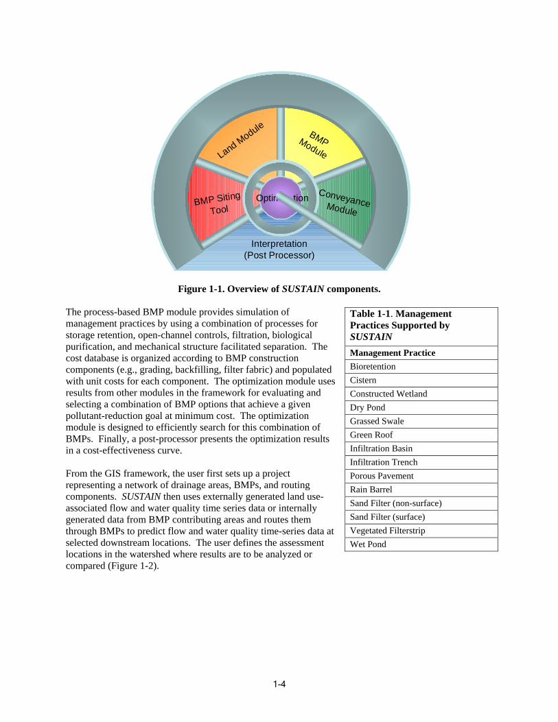
Figure 1-1 shows a generalized schematic of the overall framework. The ArcGIS-based Framework Manager (FM) is the overarching component that manages the data exchanges between the framework components. It provides linkages between external inputs, the land simulation, the BMP simulation, the conveyance simulation, the optimization module, and the post-processor. The FM checks for necessary data requirements before calling for simulation and optimization components.

Each module in the framework serves a specific function and is typically applied in series. The application usually begins with the use of the BMP siting tool, which uses the ArcGIS platform and user-guided rules to determine site suitability for various BMP options (Table 1-1). The land simulation module is used to generate runoff time series data to drive the BMP simulation. The conveyance module provides routing capabilities between land segments or BMPs or both. Users also have the option to import time series data from external watershed models (e.g., Hydrologic Simulation Program Fortran (HSPF) or Stormwater Management Model (SWMM)) instead of performing new land simulations in SUSTAIN.

1-3

ConMBMP Siting

Land Module BMPModule

veyoduTool

ancele

Interpretation (Post Processor)

Optim tion

Figure 1-1. Overview of SUSTAIN components.

The process-based BMP module provides simulation of management practices by using a combination of processes for storage retention, open-channel controls, filtration, biological purification, and mechanical structure facilitated separation. The cost database is organized according to BMP construction components (e.g., grading, backfilling, filter fabric) and populated with unit costs for each component. The optimization module uses results from other modules in the framework for evaluating and selecting a combination of BMP options that achieve a given pollutant-reduction goal at minimum cost. The optimization module is designed to efficiently search for this combination of BMPs. Finally, a post-processor presents the optimization results in a cost-effectiveness curve.

From the GIS framework, the user first sets up a project representing a network of drainage areas, BMPs, and routing components. SUSTAIN then uses externally generated land use-associated flow and water quality time series data or internally generated data from BMP contributing areas and routes them through BMPs to predict flow and water quality time -series dat a at selected downstream locations . The user defines the assessment locations in the watershed whe re results are to be analyzed or compared (Figure 1-2).

Table 1-1. Management Practices Supported by SUSTAIN Management Practice Bioretention Cistern Constructed Wetland Dry Pond Grassed Swale Green Roof Infiltration Basin Infiltration Trench Porous Pavement Rain Barrel Sand Filter (non-surface) Sand Filter (surface) Vegetated Filterstrip Wet Pond

1-4

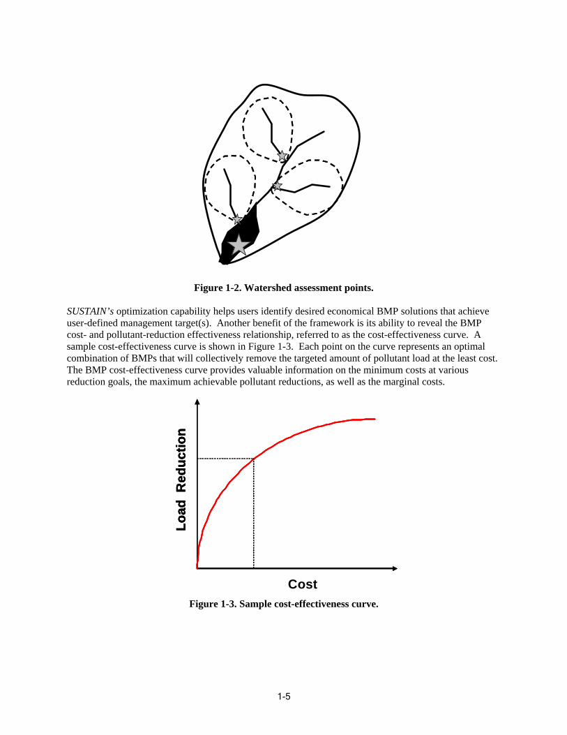
Figure 1-2. Watershed assessment points.

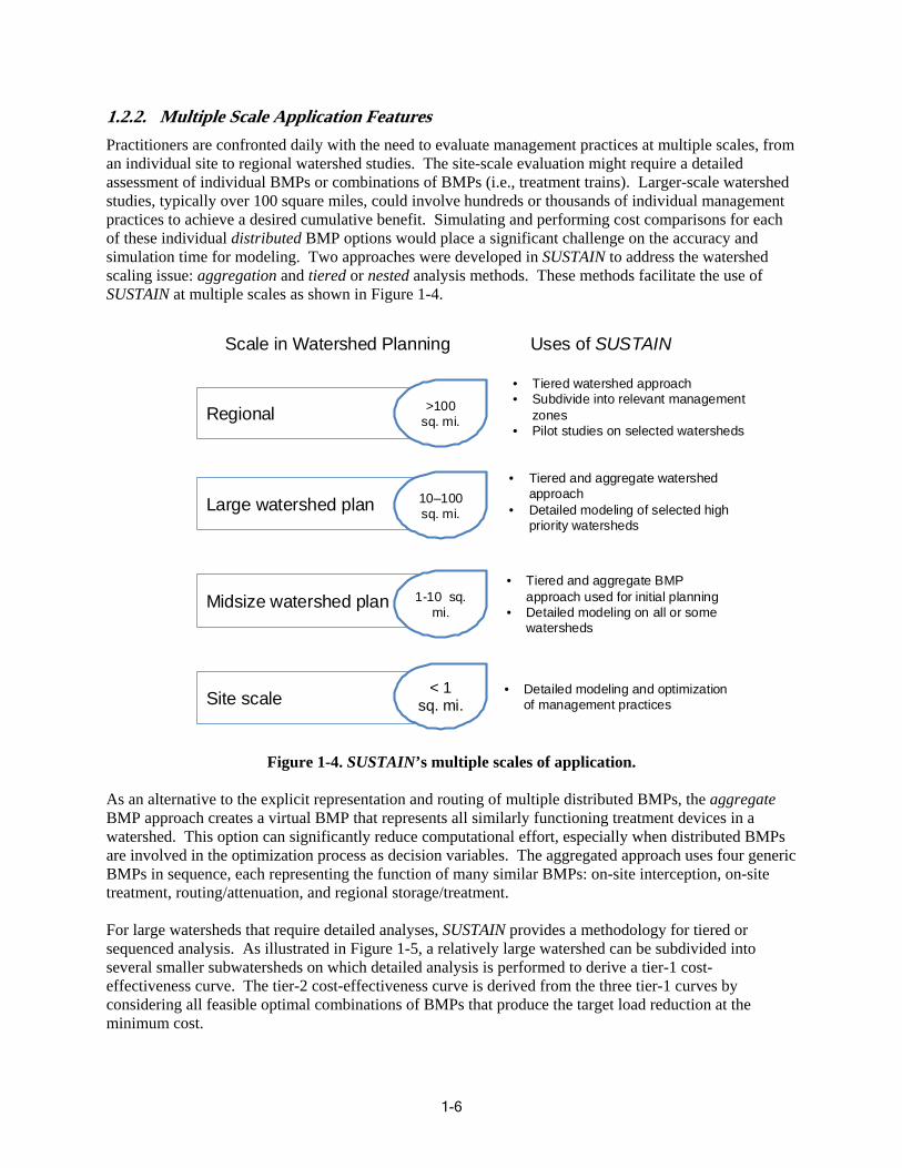
SUSTAIN’s optimization capability helps users identify desired economical BMP solutions that achieve u ser-de fi ned management target(s). Another benefit of the framework is its ability to reveal the BMPcost- and pollutant-reduction effectiveness relationship, referred to as the cost-effectiveness curve. A sample cost-effectiveness curve is shown in Figure 1-3. Each point on the curve represents an optimal combination of BMPs that will collectively remove the targeted amount of pollutant load at the least cost. The BMP cost-effectiveness curve provides valuable information on the minimum costs at various reduction goals, the maximum achievable pollutant reductions, as well as the marginal costs.

Load

Red

uctio

nLo

ad R

educ

tion

Load

Red

uctio

n

CostFigure 1-3. Sample cost-effectiveness curve.

1-5

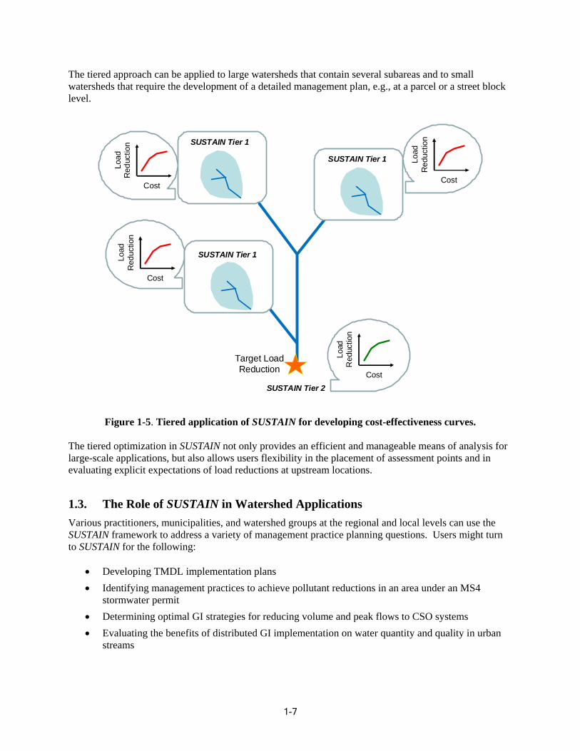
1.2.2. Multiple Scale Application Features Practitioners are confronted daily with the need to evaluate management practices at multiple scales, from an individual site to regional watershed studies. The site-scale evaluation might require a detailed assessment of individual BMPs or combinations of BMPs (i.e., treatment trains). Larger-scale watershed studies, typically over 100 square miles, could involve hundreds or thousands of individual management practices to achieve a desired cumulative benefit. Simulating and performing cost comparisons for each of these individual distributed BMP options would place a significant challenge on the accuracy and simulation time for modeling. Two approaches were developed in SUSTAIN to address the watershed scaling issue: aggregation and tiered or nested analysis methods. These methods facilitate the use of SUSTAIN at multiple scales as shown in Figure 1-4.

Scale in Watershed Planning Uses of SUSTAIN

Regional >100 sq. mi.

• Tiered watershed approach • Subdivide into relevant management

zones • Pilot studies on selected watersheds

Large watershed plan

Midsize watershed plan

Site scale

10–100 sq. mi.

1-10 sq. mi.

< 1 sq. mi.

• Tiered and aggregate watershed approach

• Detailed modeling of selected high priority watersheds

• Tiered and aggregate BMP approach used for initial planning

• Detailed modeling on all or some watersheds

• Detailed modeling and optimization of management practices

Figure 1-4. SUSTAIN’s multiple scales of application.

As an alternative to the explicit representation and routing of multiple distributed BMPs, the aggregate BMP approach creates a virtual BMP that represents all similarly functioning treatment devices in a watershed. This option can significantly reduce computational effort, especially when distributed BMPs are involved in the optimization process as decision variables. The aggregated approach uses four generic BMPs in sequence, each representing the function of many similar BMPs: on-site interception, on-site treatm nt, routing/attenuation, and regional storage e /treatment.

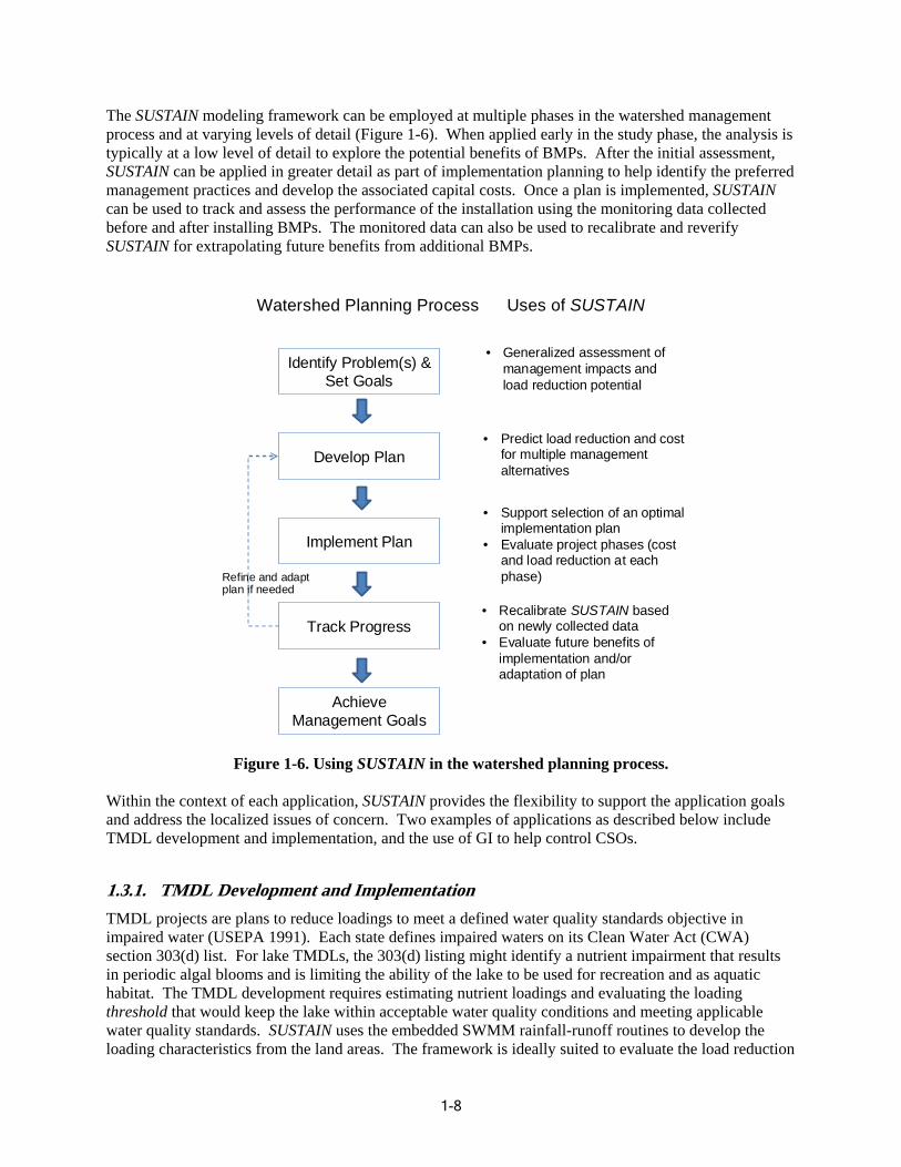
For large watersheds that re quire detailed analyses, SUSTAIN provides a methodology for tiered or sequen c ed analysis. As illustrated in Figure 1-5, a relatively large watershed can be subdivided i nto several smaller subwatersheds on which detailed analysis is performed to derive a tier-1 cost­effe cti veness curve. The tier-2 cost-effectiveness curve is derived from the three tier-1 curves by considering all feasible optimal combinations of BMPs that produce the target load reduction at the minimum cost.

1-6

The tiered approach can be applied to large watersheds that contain several subareas and to small watersheds that require the development of a detailed management plan, e.g., at a parcel or a street block level.

Cost

Red

uc

Load tio

n

Cost

ReLo

addu

ctio

n SUSTAIN Tier 1

SUSTAIN Tier 1

Load tio

n R

educ SUSTAIN Tier 1

Cost

Target Load Reduction

SUSTAIN Tier 2 Cost

Load

R

educ

tion

Figure 1-5. Tiered application of SUSTAIN for developing cost-effectiveness curves.

The tiered optimization in SUSTAIN not only provides an efficient and manageable means of analysis for large-scale applications, but also allows users flexibility in the placement of assessment points and in evaluating explicit expectations of load reductions at upstream locations.

1.3. The Role of SUSTAIN in Watershed Applications Various practitioners, municipalities, and watershed groups at the regional and local levels can use the SUSTAIN framework to address a variety of management practice planning questions. Users might turn to SUSTAIN for the following:

• Developing TMDL implementation plans • Identifying ma nagement practices to achieve pollutant reductions in an area under an MS4

stormwater permit • Determining optimal GI strategies for reducing volume and peak flows to CSO systems • Evaluating the benefits of distributed GI implementation on water quantity and quality in urban

streams

1-7

The SUSTAIN modeling framework can be employed at multiple phases in the wa tershed management process and at varying levels of detail (Figure 1-6). When applied early in the study phase, the analysis is typically at a low level of detail to explore the potential benefits of BMPs. After the initial assessment, SUSTAIN can be applied in greater detail as part of implementation planning to help identify the prefe rred management practices and develop the associated capital costs. Once a plan is implemented, SUSTAIN can be used to track and assess the performance of the installation using the monitoring data collected before and after installing BMPs. The monitored data can also be used to recalibrate and reverify SUSTAIN for extrapolating future benefits from additional BMPs.

Watershed Planning Process Uses of SUSTAIN

• Generalized assessment of management i mpacts and load reduction potential

Identify Problem(s) & Set Goals

Develop Plan

Implement Plan

Track Progress

Achieve Management Goals

Refine and adaptplan if needed

• Predict load reduction and cost for multiple management alternatives

• Support selection of an optimal implementation plan

• Evaluate project phases (cost and load reduction at each phase)

• Recalibrate SUSTAIN based on newly collected data

• Evaluate future benefits of implementation and/or adaptation of plan

Figure 1-6. Using SUSTAIN in the watershed planning process.

Within the context of each application, SUSTAIN provides the flexibility to support the application goals and address the localized issues of concern. Two examples of applications as described below include TMDL development and implementation, and the use of GI to help control CSOs.

1.3.1. TMDL Development and Implementation TMDL projects are plans to reduce loadings to meet a defined water quality standards objective in impaired water (USEPA 1991). Each state defines impaired waters on its Clean Water Act (CWA) section 303(d) list. For lake TMDLs, the 303(d) listing might identify a nutrient impairment that results in periodic algal blooms and is limiting the ability of the lake to be used for recreation and as aquatic habitat. The TMDL development requires estimating nutrient loadings and evaluating the loading threshold that would keep the lake within acceptable water quality conditions and meeting applicable water quality standards. SUSTAIN uses the embedded SWMM rainfall-runoff routines to develop the loading characteristics from the land areas. The framework is ideally suited to evaluate the load reduction

1-8

potential as part of examining the reasonable assurance that the TMDL can be achieved at the prescribed load reductions. After the TMDL is developed, SUSTAIN can be used to develop the implementation plan that identifies the best combination of management practice type(s) and location(s), and the associated cost load reductions.

In some areas, TMDL implementation is addressed by a municipal stormwater permit. For communities working to comply with wasteload allocations assigned in a TMDL, SUSTAIN provides a method to integrate stormwater permit activities with the requirements of the TMDL. Capitalizing on mapping and data collection activities typically undertaken as part of the MS4 implementation, SUSTAIN can be used to enumerate specific measures necessary for meeting TMDL reductions throughout the affected area. The framework can be used to pinpoint the best locations for optimizing pollutant reductions and to determine the mix of management practices that will achieve necessary load reductions for the least cost.

Examples of the TMDL-related investigations that SUSTAIN supports include the following:

• Optimizing the geographic focus of management activities (near the waterbody of concern or away from it)

• Evaluating the benefits of installing rain barrels or rain gardens in a near-lake region • Enumerating specific management practices that must be implemented to satisfy the TMDL • Developing a funding request • Developing a projection of reduction potential for phased installation over time

1.3.2. Evaluation of GI Practices as Part of a CSO Control Program Even with advances in sewer technology (e.g., sewer separation and deep sto rage), problems still remain with the operation of existing urban wastewater systems (NRDC 2006). Examples include impaired performance of wastewater treatment plants resulting from the influx of stormwater (infiltration and inflow), constraints on urban growth caused by an inadequate infrastructure, and aging combined sewer systems, which can require costly rehabilitation (USEPA 2004). CSO control programs typically focus on infiltrating or storing runoff to minimize peak flows to collection systems and reduce the frequency and size of overflow events. Programs are developed and implemented to comply with mandated CSO long-term control plans. Such challenges have led to the development of sustainable strategies for urban stormwater and wastewater management and new alternatives to the traditional centralized sewer systems, which comprise laterals, submains, and trunk lines all leading to a central treatment facility (Chocat et al. 2007). Although large storage structures, tunnels, and sewer separation have been used successfully to significantly reduce CSOs in major cities, increased effectiveness and multiple benefits can be derived by adopting new GI approaches in combination with traditional approaches.

As a means to redu ce volume entering a wastewater system and reduce its peak flows, GI can be applied through source controls and engineered BMP systems to infiltrate, evapotranspirate, or store stormwater runoff for beneficial uses (USEPA 2007). Those approaches are to keep stormwater run off from entering a combined sewer system and reduce o verflows (USEPA 2004). In addition, many GI approaches can be included in adaptive management strategies designed to be resilient to su ch system changing factors as population growth and climate change (USEPA 2008).

SUS TA IN is designed to support linkage to other related models such as detailed sewer system models or receivi ng water models of affected rivers, lakes, and estuaries. Where existing sewer and watershed models are av ailable, SUSTAIN can be used to predict the most inexpensive GI practices that will result in reduced overflow volumes and frequency.

1-9

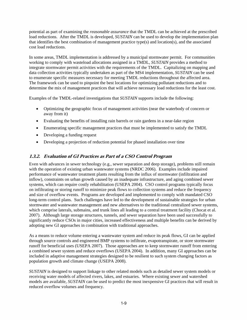
1.4. SUSTAIN Application Process A typical SUSTAIN application scenario begins with the definition of study objectives, followed by data coll iect on, project/model setup, formulation of the optimization problem, and analysis of results. Figure1-7 is a flow dia gram illustrating the typical step-by-step process in SUSTAIN applications.

Def

ine

-Wha

t que

sap

b ti

b

plic

atio

n o

ons

need

to je

ctiv

es:

e an

swer

ed?

Data Collection & Analysis • Study area review • GIS data: land use, stream, DEM, BMP sites, etc. • Watershed and BMP information/data • Compile monitoring data (calibration/validation)

Project Setup • BMP representation: placement, configuration, and cost • Land/Watershed Representation • Routing network • Assessment point(s) • Test system application (externally calibrated model) • Calibrate/validate model (internal model)

Put Optimization Processor to Work • Select decision variables (BMP dimensions) • Select assessment points (BMP/Outlet locations) • Select evaluation factors, control targets (end points)

Results Analysis and Representation (Post-Processor) • Optimum BMP dimensions • Alternate solutions

Figure 1-7. SUSTAIN application process.

Fundamental to the setup and application of SUSTAIN is a clear definition of the study objective(s)— What is the question that is to be answered by the analysis? For example, the objective of the study might be to identify the set of management options (including both site- and regional-scale techniques) that achieve a required level of pollutant load reduction (i.e., annual load in lbs/yr). For a CSO study, the objective might be stated as, “to reduce frequency of overflow through extensive retrofit of the drainage area.” The reduction in overflow can be measured by the magnitude of peak flows in a collection system. The study objectives will define the scope and extent of the SUSTAIN application, which could include the areas to be modeled, runoff and pollutant factors to be simulated, additional data collection needs, the locations where the output will be evaluated (i.e., assessment points), and the determination of the optimization evaluation factors and control targets (i.e., endpoints). At each control target, SUSTAIN is capable of producing outputs in various time averaging periods and frequencies of occurrences that will facilitate the evaluation and comparison of management alternatives. The following lists the examples of output variations.

• Average annual flow volume percent reduction based on an existing condition • Average annual flow volume • High-flow rate and allowed maximum duration (user specified)

1-10

• Peak-flow value and maximum exceedance frequency • Average annual sediment/pollutant load percent reduction with respect to an existing condition • Average annual sediment/pollutant load (load target) • Average sediment/pollutant concentration (the maximum average concentration allowed) • High sediment/pollutant concentration and duration (concentration thresh old value and allowed

maxim um duration when concentration exceeds the threshold) • Long-term average sediment/pollutant loa d (daily, monthly, annual, or any user specified time

frame) • Exceedance frequency (the threshold value and maximum exceedance frequency allowed)

SUSTAIN has been design d with inherene t flexibility in the form ulation and setup of the application. The careful definition of the project objective, associated evaluation factors, and control targets will ensure the most appr opria te and useful application.

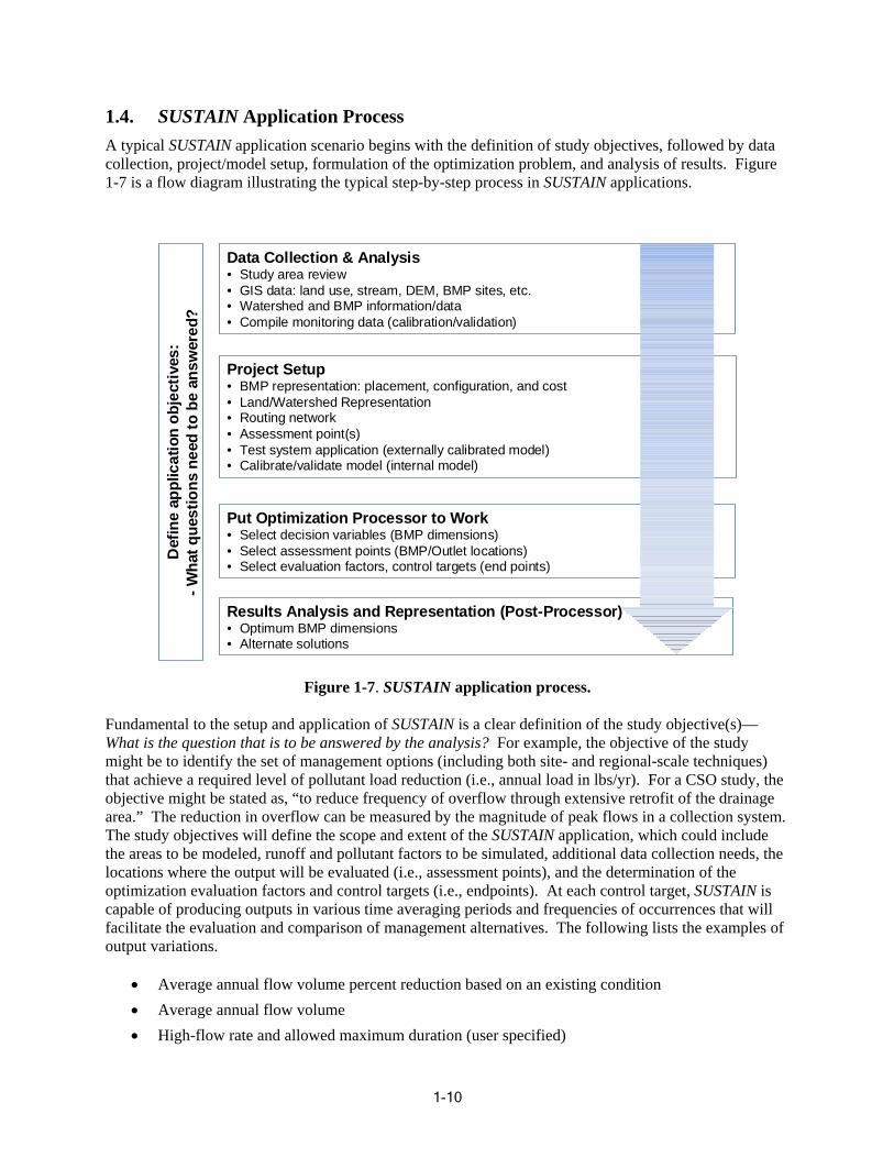
The data collection process for a SUSTAIN application is similar to most modeling projects and in volves a thorough compilation and review of information a vaila ble for the study area. It generally includ es gathering applicable regional and site-scale GIS da ta la yers, digital elevation model (DEM) data, stream networks, locations of BMPs, land use data, critical so urce information, and monitoring data for calibration and validation. A summa ry of typical data needs is shown in Table 1-2.

Setting up th e SUSTAIN pro ject involves using the data collected to establish a representation of the land and pollutant so urces in the watershed as well as the ro uting network, assessment points, and man agement practices to be evaluated. For site-scale analysis of ma nagement practices, locally derived higher-resolution site scale data will likely be required.

If the continuous time series data of flow and associa ted sedim ent/pollutants from a locally calibrated model study is available, the data can be imported into SUSTAIN without recreating them. Most models that operate on an hourly or shorter time step, such as HSPF, SWMM, Source Loading and Managem ent Model for Windows (WINSLAMM), are compatible w ith SUSTAIN. When importing information from an externally generated model, the SUSTAIN application builds on the documentation, testing, calibration, and validation of the external model.

After project setup, the opti mization m odule synthesize s information from the BMP, land, and conveyan ce modules and generates solutions that are lo oped back for evaluation using the sam e modules again. Via this evolutionary search process, the optimi zer identifies the best or most cost-effective BMP solutions according to the user’s specific conditions and objectives. Finally, the post-processor analyzes optimization results using specific graphical and tabular reports that facilita te the classification of storm events for analysis, viewi ng the time series of s pecific storm events, evaluating BMP performan ce by storm event, and developin g the cost-effectiveness c urves for treatment alternatives.

1-11

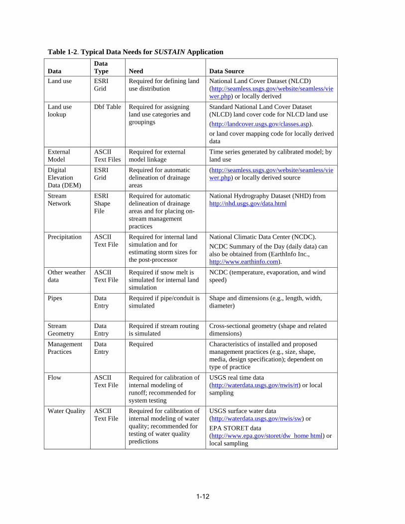
Table 1-2. Typical Data Needs for SUSTAIN Application

Data Data Type Need Data Source

Land use ESRI Grid

Required for defining land use distribution

National Land Cover Dataset (NLCD) (http://seamless.usgs.gov/website/seamless/vie wer.php) or locally derived

Land use okup lo

Dbf Table Required for assigning land use categories and groupings

Standar d National Land Cover Dataset (NLCD) land cover code for NLCD land use (http://landcover.usgs.gov/classes.asp). or land cover mapping code for locally derived data

Exte Mod

rnal el

ASCII Text Files

Required for external model linkage

by land use Time series generated by calibrated model;

Dig Elev Dat

ital ation

a (DEM)

ESRI Grid

Required for automatic delineation of drainage areas

(http://seamless.usgs.gov/website/seamless/vie wer.php) or locally derived source

Stre Net

am work

ESRI Shape File areas and for placing on-

Required for automatic delineation of drainage

stream management practices

National Hydrography Dataset (NHD) from http://nhd.usgs.gov/data.html

Precipitation ASCII Text File

Required for internal land simulation and for estimating storm sizes for the post-processor

National Climatic Data Center (NCDC). NCDC Summary of the Day (daily data) can also be obtained from (EarthInfo Inc., http://www.earthinfo.com).

Other weather data

ASCII Text File

Required if snow melt is simulated for internal land simulation

NCDC (temperature, evaporation, and wind speed)

Pipes Data Entry

Required if pipe/conduit is simulated

Shape and dimensions (e.g., length, width, diameter)

Stream Geometry

Data Entry

Required if stream routing is simulated

Cross-sectional geometry (shape and related dimensions)

Management Practices

Data Entry

Required Characteristics of installed and proposed management practices (e.g., size, shape, media, design specification); dependent on type of practice

Flow ASCII Text File

Required for calibration of internal modeling of runoff; recommended for system testing

USGS real time data (http://waterdata.usgs.gov/nwis/rt) or local sampling

Water Quality ASCII Text File

Required for calibration of internal modeling of water quality; recommended for testing of water quality predictions

USGS surface water data (http://waterdata.usgs.gov/nwis/sw) or EPA STORET data (http://www.epa.gov/storet/dw home html) or local sampling

1-12

1.5. About this Report This report provides the description and documentation to support the release of of SUSTAIN Version 1.0. As it is developed, EPA will release additional model information on the SUSTAIN Web site. The Web site also provides user guidance and responses to frequently asked questions regardin g the operation and use of the model.

This SUSTAIN documentation report is organized as follows:

Chapter 1 provides a general overview of the framework, its development, typical applications, and application process.

Chapter 2 describes the structure of the framework, the roles and interactions of its major components, and its operational characteristics.

Chapter 3 provides the detailed documentation of the analytical procedures and simulation processes, including equations and variables, which are adopted and incorporated into various parts of SUSTAIN.

Chapter 4 presents two case studies to demonstrate how the framework is applied for selection and placement of BMPs.

The appendices include a needs analysis f or developing a comprehensive placement framework, a review of land and BMP simulation models, and a summary of expert opinions on the current state­of-the-art in optimization concepts and methods to support development of the optimization component in SUSTAIN. It includes the rationale and supporting information used in formulating the framework design and selecting land and BMP simulation techniques that appear in SUSTAIN.

1-13

Chapter 2 SUSTAIN Design and Structure SUSTAIN is a comprehensive, multiscale watershed and water quality modeling application built on an ArcGIS platform linked to multiple simulation modules, an optimization module, and a post-processo r, which analyzes and helps interpret the results. The modular design of SUSTAIN has multiple a dvantages compared to previous modeling applications including the ability to incorporate simulation of new management practices as they are evolved, to operate independently for specific small watershed applications, and to provide flexibility to address multiple watershed scales.

This chapter describes the system’s infrastructure, its major modules, and software platforms. It also explains how they are linked and interact.

The SUSTAIN installation requires ESRI’s ArcGIS 9.3 and the Spatial Analyst extension. The application is compatible with Microsoft Windows 98, 2000, NT, XP, and Vista operating systems and requires at least 1GB of computer me mory and 5GB of free space on the hard disk. The sys tem also requires Microsoft Excel 2003, which is used as a post-processor for analyzing and interpreting results.

SUSTAIN comprises the following modules:

Fr amework Manager—to serve as the command module of SUSTAIN, manage data for system functions, provide linkages between the system modules, and create a simulation network to guide the mo deling and optimization activities

Land module—to generate runoff and pollutant loads from the land through internal land simulatio n or importing precalibrated land simulation time series

BMP module—to perform process simulation of flow and water quality through BMPs

Conveyance module—to perform routing of flow and water quality in a pipe or a channel

Optimization module—to evaluate and identify cost-effective BMP placement and selection strategies for a preselected list of potential sites, applicable BMP types, and ranges of BMP size

Po s t-Processor—to perform analysis and summarization of the simulation results for decision making

2.1. Framework Manager The FM performs data management, spatial analysis, and network visualization. It integrates components from the GIS network, such as stre ams, conduits, and land uses, with relevant simulation modules, draws external time series data (e.g., rainfall, runoff) as required, and checks for necessary data requirement s before calling for simulation and optimization components.

SUSTAIN is designed to interactively identify and manage the re quired databases, including geographic and tabular data sets. The primary function of data management is to define the paths where data are stored and to identify required data elements. SUSTAIN provides the option to store required geographic

2-14

data on the hard disk or in a file-based geodatabase, which is a native data structure used by ArcGIS. The geodatabase is composed of tables and queries that allow data sharing and interchange among SUSTAIN’s modules. The FM builds on the ESRI ArcGIS (version 9.3) platform to support the placement of BMPs, delineation of BMP tributary drainage areas and flow paths, and development of a schematized watershed simulation network that might include land parcels, management practices, and stream reaches. The GIS component also se rves as the user interface and includes the main application window with menus, buttons, and dialog boxes. The GIS interface allows a user to read and edit spatial and temporal data sets.

All commonly used Microsoft Office applications can be easily linked to the platform. Microsoft Excel, a popular and powerful application for displaying and manipulating simulation time series data and scientific graphics, was chosen as the post-processor for SUSTAIN.

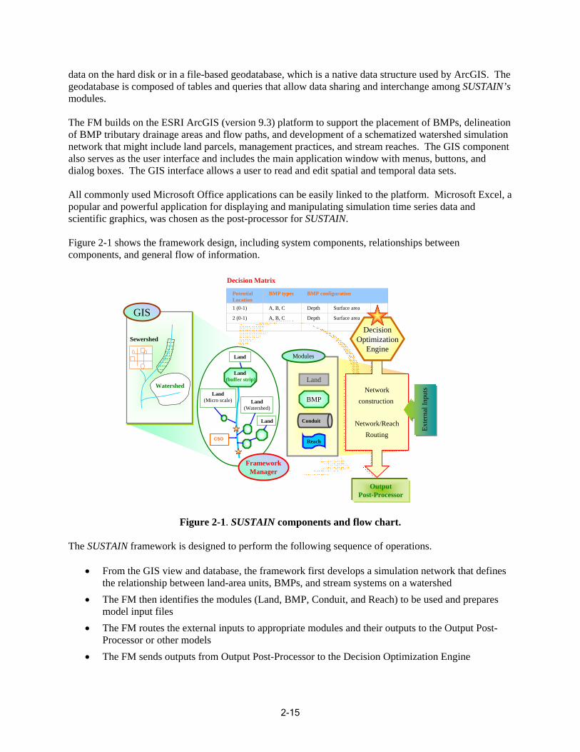
Figure 2-1 shows the framework design, including system components, relationships between components, and general flow of information.

Figure 2-1. SUSTAIN components and flow chart.

The SUSTAIN framework is designed to perform the following sequence of operations.

• From the GIS view and database, the framework first develops a simulation network that defines the relationship between land-area units, BMPs, and stream systems on a watershed

• The FM then identifies the modules (Land, BMP, Conduit, and Reach) to be used and prepares model input files

• The FM routes the external inputs to appropriate modules and their outputs to the Output Post-Processor or other models

• The FM sends outputs from Output Post-Processor to the Decision Optimization Engine

2-15

Decision Matrix

Potential BMP types BMP configuration Location 1 (0-1) A, B, C Depth Surface area GIS 2 (0-1) A, B, C Depth Surface area

Decision Sewershed Optimization

Engine Land Modules

Land (buffer strip) Land

Watershed NetworkLand BMP(Micro scale) Land construction

(Watershed)

Land Conduit Network/ReachRouting

CSO Reach

Framework Manager

Output Post-Processor

Exte

rnal

Inpu

ts

• The Optimization Engine evaluates the current option and selects the next preferred option from that contained in the Feasible Option Matrix on the basis of cost and defined flow and waterquality criteria. The preferred option can be a different combination of BMP locations and types. The Feasible Option Matrix contains types, configurations, locations, and costs of feasible BMP options

• SUSTAIN performs numerous iterations of the sequence until the user-defined convergence criteria are met

• The tool does not automatically select the best solution but is expected to be used as a tool to explore and test various approaches and eventually select optimal solutions on the basis of user-defined criteria and constraints

2.2. Simulation Modules SUSTAIN’s modular simu lation core consists of three standalone simulation modules: the landscape simu lation module (Land), the standalone BMP module (BMP), and a conveyance simulation module (Conduit and Reach) as shown in the central box o f F igure 2-1.

To provide a seamless and efficient operation, SUSTAIN selects and incorporates simulation routines from commonly used watershed and receiving water models (e.g., SWMM (Huber and Dickinson 1988), HSPF (Bicknell 2001), and Loading Simulation Program—C++ (LSPC) (Tetra Tech and USEPA 2002). The following is a summary list of simulation routines and the model where the routines were adopted:

• Watershed/landscape models: SWMM’s atmospheric, land surface, and groundwat er compartments

• Conveyance and pollutant routing: in HSPF/LSPC RCHRES and SWMM Transport compartment • BMP simulation m odels: Prince George’s County BMP module (Tetra Tech 2001 ) and selected

buffer zone simulation techniques from the VFSMOD (Munoz-Carpena and Parsons 2003)

The VFSMOD is programmed in FORTRAN computer lan guage and compiled as a standalone d ynamic link library, whereas other simulation modu les are coded in the visual C++ programming language.

The standalone simulati on modules are packaged within SUSTAIN to perform the generation and transport of sediment and other pollutants at th e source (land use type), in the BMP, and in the convey ance system. Table 2-1 shows the inte raction betwee n the Land, BMP, and Conveyance m odules to handle transport of sediment in SUSTAI N. It shows the inputs, the methods used to simulate the sedimen t transport, and the resulting o utputs from these simu lation modules. Table 2-2 shows the interaction between the Land, BMP, and Co nveyance modu les to handle transport of other pollut ants in SUSTAIN. It also shows the inputs, the methods used to simu late the water quality processes, and the resulting outputs from the simulation mo dules.

2-16

↓

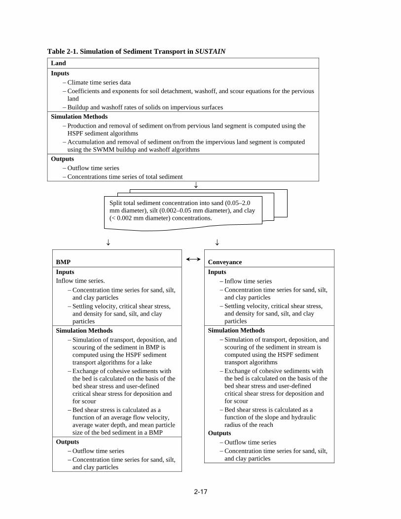
BMP Inpu ts Inflow time series .

− Concentration time series for sand, silt, and clay particles

− Settling velocity, critical shear stre ss, and density for sand, silt, and clay particles

Simulation Methods − Simulation of transport, deposition, an d

scouring of the sediment in BMP is computed using t he HSPF sediment transport algorithms for a lake

− Exchange of cohesive sediments wi th the bed is calculated on the basis o f the bed shear stress and user-de fined critical shear stress for deposition and for scour

− Bed shear stress is calculated as a function of an average flow velocity, aver age water depth, and mean particle size of the bed sedime nt in a BMP

Out puts − Outflow time series − Concentration time series for sand, silt,

and clay particles

↓ ↓ Conveyance Inputs

− In flow time s eries − Concentration time series for sand, silt,

and clay particles − Se ttling velocity, critical shear stres s,

an d density for sand, silt, and clay pa rticles

Simul ation Methods − Si mulation of transport, deposition, a nd

scourin g of the sediment in stream is compu ted using the HSPF sediment transport algorithms

− Exchange of cohesive sediments wit h th e bed is calculated on the basis of the bed shear stress and user-defined critical shear stress for deposition and for scour

− Bed shear stress is calculated as a function of the slope and hydraulic radius of the reach

Outputs − Outflow time series − Concentration time series for sand, silt,

and clay particles

Table 2-1. Simulation of Sediment Transport in SUSTAIN Land Inputs

− Clim series data − Coefficie etachment, washoff, and scour equations for the pervious

land − Buildup an pervious surfaces

ate time nts and exponents for soil d

d washoff rates of solids on im Simulation

− Productio g the HSPF sedi

− Accumulat using the S lgorithms

Methods n and removal of sediment on/from pervious land segment is computed usin ment algorithms ion and removal of sediment on/from the impervious land segment is computed WMM buildup and washoff a

Outputs − Outflow tim − Concentrat

e series ions time series of total sediment

Split total sediment concentration into sand (0.05–2 .0 mm diameter), silt (0.002–0.05 mm diameter), an d clay (< 0.002 mm diameter) concentr a tions.

2-17

↓ ↓

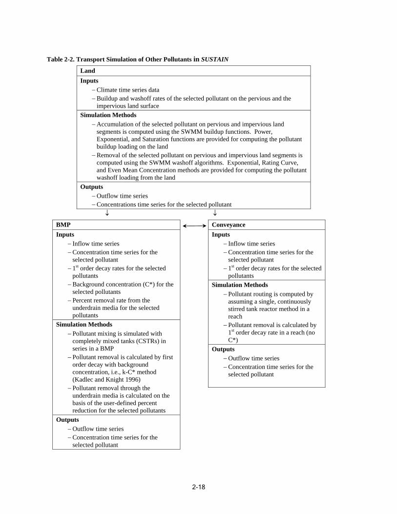
Table 2-2. Transport Simulation of Other Pollutants in SUSTAIN

Land Inputs

− Climate time series data − Buildup and washoff rates of the selected pollutant on the pervious and the

impervious land surface Simulation Methods

elected pollutant on pervious and impervious land segments is

− Accumulation of the selected pollutant on pervious and impervious land segments is computed using the SWMM buildup functions. Power, Exponential, and Saturation functions are provided for computing the pollutant buildup loading on the land

− Removal of the s computed using the SWMM washoff algorithms. Exponential, Rating Curve, and Even Mean Concentration methods are provided for computing the pollutant washoff loading from the land

Outputs − Outflow time series − Concentrations time series for the selected pollutant

BMP Inputs

− Inflow time series − Concentration time series for the

selected pollutant − 1st order decay rates for the selected

pollutants − Background concent

sele ration (C*) for the

cted pollutants − Percent removal rate from the

underdrain media for the selected pollutants

Simulation Methods − Pollutant mixing is simulated with

completely mixed tanks (CSTRs) in series in a BMP

− Pollutant removal is calculated by first order decay with background concentration, i.e., k-C* method (Kadlec and Knight 1996)

− Pollutant removal through the underdrain media is calculated on the basis of the user-defined percent reduction for the selected pollutants

Outputs − Outflow time series − Concentration time series for the

selected pollutant

Conveyance Inputs

− Inflow time series − Concentration time series for the

selected pollutant − 1st order decay rates for the selected

pollutants Simulation Methods

− Pollutant routing is computed by assuming a single, continuously stirred tank reactor method in a reach

− Pollutant removal is calculated by 1st order decay rate in a reach (no C*)

Outputs − Outflow time series − Concentration time series for the

selected pollutant

2-18

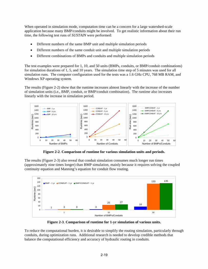
When operated in simulation mode, computation time can be a concern for a large watershed-scale application because many BMP/conduits might be involved. To get realistic information about their run time, the following test runs of SUSTAIN were performed:

• Different numbers of the same BMP unit and multiple simulation periods • Different numbers of the same conduit unit and multiple simulation periods • Different combinations of BMPs and conduits and multiple simulation periods

The test examples were prepared for 1, 10, and 50 units (BMPs, conduits, or BMP/conduit combin ations) for simulation durations of 1, 5, and 10 years. The simulation time step of 5 minutes was used for a ll simulation runs. The computer configuration used for the tests was a 1.6 GHz CPU, 768 MB RAM, and Windows XP operating system.

The results (Figure 2-2) show that the runtime increases almost linearly with the increase of the number of simulation units (i.e., BMP, conduit, or BMP/conduit combination). The runtime also increases linearly w ith the increase in simulation period.

0

200

400

600

0 10 20 30 40 50 60

Number of BMPs

Ru

800

1000

1200

1400

1600

me

(sec

) nt

i

BMP - 1 yr

BMP - 5 yrs

BMP - 10 yrs

0

200

400

600

0 10 20 30 40 50 60

Number of Conduits

Run

t

800

1000

1200

1400

1600

me

(sec

) i

CONDUIT - 1 yr CONDUIT - 5 yrs

CONDUIT - 10 yrs

0

200

400

600

0 10 20 30 40 50 60

Number of BMPs/Conduits

Run

800ime

( 1000

1200

1400

1600

sec)

BMP/CONDUIT - 1 yr BMP/CONDUIT - 5 yrs

BMP/CONDUIT - 10 yrs

Figure 2-2. Comparison of runtime for various simulation units and periods.

The results (Figure 2-3) also reveal that conduit simulation consumes much longer run times (approximately nine times longer) than BMP simulation, mainly because it requires solving the coupled continuity equation and Manning’s equation for conduit flow routing.

160

133 135

100

120

140

sec)

BMP - 1 yr CONDUIT - 1 yr BMP/CONDUIT - 1 yr

1 3 16

3

25

3

27

0

20

40

1 10

60

80

Run

time

(

50 Number of BMPs/Conduits

Figure 2-3. Comparison of runtime for 1-yr simulation of various units.

To reduce the computational burden, it is desirable to simplify the routing simulation, particularly t hrough conduits, during optimization runs. Additional research is needed to develop credible methods that balance the computational efficiency and accuracy of hydraulic routing in conduits.

2-19

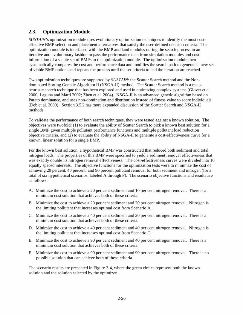
2.3. Optimization Module SUSTAIN’s optimization module uses evolutionary optimization techniques to identify the most cost-effective BMP selection and placement alternatives that satisfy the user-defined decision criteria. The optimization module is interfaced with the BMP and land modules during the search process in an iterative and evolutionary fashion to pas s the performance data from simulation modules and cost information of a viable set of BMPs to the optimization module. The optimization module then systematically compares the cost and performance data and modifies the search path to generate a new set of viable BMP options and repeats the process until the set criteria to end the iteration are reached.

Two optimization techniques are supported by SUSTAIN: the Scatter Search method and the Non-dominated Sorting Genetic Algorithm II (NSGA-II) method. The Scatter Search method is a meta­heuristic search technique that has been explored and used in optimizing complex systems (Glover et al. 2000; Laguna and Marti 2002; Zhen et al. 2004). NSGA-II is an advanced genetic algorithm based on Pareto dominance, and uses non-domination and distribution instead of fitness value to score individuals (Deb et al. 2000). Section 3.5.2 has more expanded discussion of the Scatter Search and NSGA-II methods.

To validate the performance of both search techniques, they were tested against a known solution. The objectives were twofold: (1) to evaluate the ability of Scatter Search to pick a known best solution for a single BMP given multiple pollutant performance functions and multiple pollutant load reduction objective criteria, and (2) to evaluate the ability of NSGA-II to generate a cost-effectiveness curve for a known, linear solution for a single BM P.

For the known best solution, a hypothetical BMP was constructed that reduced both sediment and total nitrogen loads. The properties of this BMP were specified to yield a sediment removal effectiveness that was exactly double its nitrogen removal effectiveness. The cost-effectiveness curves were divided into 10 equally spaced intervals. The objective functions for the optimization tests were to minimize the cost of achieving 20 percent, 40 percent, and 90 percent pollutant removal for both sediment and nitrogen (for a total of six hypothetical scenarios, labeled A through F). The scenario objective functions and results a re as follows:

A. Minimize the cost to achieve a 20 per cent sediment and 10 per cent nitrogen removal. There is a minimum cost solution that achieves both of these criteria.

B. Minimize the cost to achieve a 20 per cent sediment and 20 per cent nitrogen removal. Nitrogen is the limiting pollutant that increases optimal cost from Scenario A.

C. Minimize the cost to achieve a 40 per cent sediment and 20 per cent nitrogen removal. There is a minimum cost solution that achieves both of these criteria.

D. Minimize the cost to achieve a 40 per cent sediment and 40 per cent nitrogen removal. Nitrogen is the limiting pollutant that increases optimal cost from Scenario C.

E. Minimize the cost to achieve a 90 per cent sediment and 40 per cent nitrogen removal. There is a minimum cost solution that achieves both of these criteria.

F. Minimize the cost to achieve a 90 per cent sediment and 90 per cent nitrogen removal. There is no possible solution that can achieve both of these criteria.

The scenario results are pre sented in Figure 2-4, where the green circles represen t both the known solution and the solution selected by the optimizer.

2-20

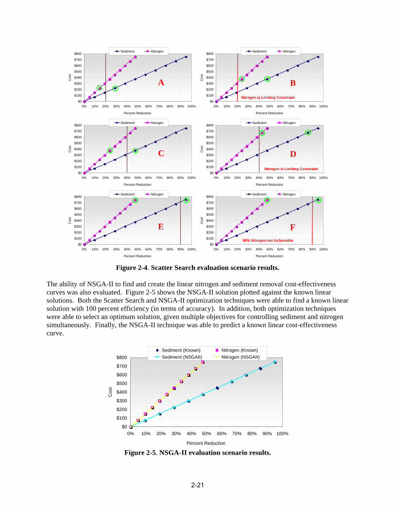
2-21

Nitrogen is Limiting Constraint

D

$800 $800

$700 $700

$600 $600

$500 $500

Sediment Nitrogen

A

0% 10% 20% 30% 40% 50% 60% 70% 80% 90% 100%

Percent Reduction

Sediment Nitrogen

Nitrogen is Limiting Constraint

B

Cos

t

Cos

t C

ost

Cos

t

Cos

t C

ost

$400

$300

$400

$300

$200 $200

$100 $100

$0 $0 0% 10% 20% 30% 40% 50% 60% 70% 80% 90% 100%

Percent Reduction

Sediment Nitrogen $800 $800

$700 $700

$600 $600

$500 $500

Sediment Nitrogen

C$400 $400

$300 $300

$200 $200

$100 $100

$0 $0 0% 10% 20% 30% 40% 50% 60% 70% 80% 90% 100% 0% 10% 20% 30% 40% 50% 60% 70% 80% 90% 100%

Percent Reduction Percent Reduction

Sediment Nitrogen

E

0% 10% 20% 30% 40% 50% 60% 70% 80% 90% 100%

Percent Reduction

Sediment Nitrogen

90% Nitrogen not Achievable

F

$800 $800

$700 $700

$600 $600

$500 $500

$400 $400

$300 $300

$200 $200

$100 $100

$0 $0 0% 10% 20% 30% 40% 50% 60% 70% 80% 90% 100%

Percent Reduction

Figure 2-4. Scatter Search evaluation scenario results.

The ability of NSGA-II to find and create the linear nitrogen and sediment removal cost-effectiveness curves was also evaluated. Figure 2-5 shows the NSGA-II solution plotted against the known linear solutions. Both the Scatter Search and NSGA-II optimization techniques were able to find a known linear solution with 100 percent efficiency (in terms of accuracy). In addition, both optimization techniques were able to select an optimum solution, given multiple objectives for controlling sediment and nitrogen simultaneously. Finally, the NSGA-II technique was able to predict a known linear cost-effectiveness curve.

$0

$100

$200

$300

$400

$500

Cos

t

$600

$700

$800 Sediment (Known) Nitrogen (Known) Sediment (NSGAII) Nitrogen (NSGAII)

0% 10% 20% 30% 40% 50% 60% 70% 80% 90% 100%

Percent Reduction

Figure 2-5. NSGA-II evaluation scenario results.

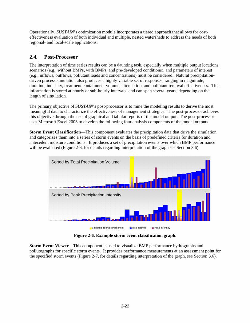
Operationally, SUSTAIN’s optimization module incorporates a tiered approach that allows for cost-effectiveness evaluation of both individual and multiple, nested watersheds to address the needs of both regional- and local-scale applications.

2.4. Post-Processor The interpretation of time series results can be a daunting task, especially when multiple output locations, scenarios (e.g., without BMPs, with BMPs, and pre-developed conditions), and parameters of interest (e.g., inflows, outflows, pollutant loads and concentrations) must be considered. Natural precipitation-driven process simulation also produces a highly variable set of responses, ranging in magnitude, duration, intensity, treatment containment volume, attenuation, and pollutant removal effectiveness. This information is stored at hourly or sub-hourly intervals, and can span several years, depending on the length of simulation.

The primary objective of SUSTAIN’s post-processor is to mine the modeling results to derive the most meaningful data to characterize the effectiveness of management strategies. The post-processor achieves this objective through the use of graphical and tabular reports of the model output. The post-processor uses Microsoft Excel 2003 to develop the following four analysis components of the model outputs.

Storm Event Classification —This component evaluates the precipitation data that drive the sim ulation and categorizes them into a series of storm events on the basis of predefined criteria f or duration and antecedent moisture conditions. It produces a set of precipitation events over which BMP performance will be evaluated (Figure 2-6, for details regarding interpretation of the graph see Section 3.6).

53%

Sorted by Total Precipitation Volume

82%

Sorted by Peak Precipitation Intensity

Selected Interval (Percentile) Total Rainfall Peak Intensity

Figure 2-6. Example storm event classification graph.

Storm Event Viewer—This component is used to visualize BMP performance hydrographs and pollutographs for specific storm events. It provides performance measurements at an assessment point for the specified storm events (Figure 2-7, for details regarding interpretation of the graph, see Section 3.6).

2-22

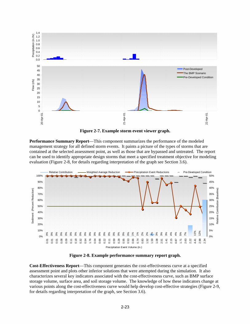
2-23

0.0 0.2 0.4 0.6 0.8 1.0 1.2 1.4

Pre

cipi

tatio

n (in

./hr)

0 5

10

15 20 25 30 35

40 45 50

Flow

(cfs

)

Post-Developed The BMP Scenario Pre-Developed Condition

20-A

pr-0

1

21-A

pr-0

1

22-A

pr-0

1

Figure 2-7. Example storm event viewer graph.

Performance Summary Report—This component summarizes the performance of the modeled management strategy for all defined storm events. It paints a picture of the types of storms that are contained at the selected assessmen t point, as well as those that are bypassed and untreated. The report can be used to identify appropriate design storms that meet a specified treatment objective for modeling evaluation (Figure 2-8, for details regarding interpretation of the graph see Section 3.6).

10%

0%

Relative Contribution Weighted Average Reduction Precipitation Event Reductions Pre-Developed Condition 100% 50%

90% 45%

0% 0% 0% 0% 0% 0% 0% 0% 0% 0% 0% 0% 0% 0% 0% 0% 0% 0% 1% 1% 2% 2% 2% 3% 3% 3% 4% 4% 5% 7% 11%

12%

Sed

imen

t (P

erce

nt R

ed uc

tion) 80%

70%

60%

50%

40%

30%

20%

40%

35%

30%

25%

20%

15%

10%

5%

0%

Rel

ativ

e C

ontri

butio

n (B

asel

in e)

0.01

0.01

0.01

0.08

0.09

0.11

0.18

0.32

0.54

1.76

0.04

0.66

0.22

0.11

0.59

0.28

0.55

0.53

0.66

0.74

0.83

1.52

1.59

1.08

2.51

1.41

2.15

0.87

1.71

2.63

2.22

4.41

2.98

2.34

Precipitation Event Volume (in.)

Figure 2-8. Example performance summary report graph.

Cost-Effectiveness Report—This component generates the cost-effectiveness curve at a specified assessment point and plots other inferior solutions that were attempted during the simulation. It also characterizes several key indicators associated with the cost-effectiveness curve, such as BMP surface storage volume, surface area, and soil storage volume. The knowledge of how these indicators change at various points along the cost-effectiveness curve would help develop cost-effective strategies (Figure 2-9, for details regarding interpretation of the graph, see Section 3.6).

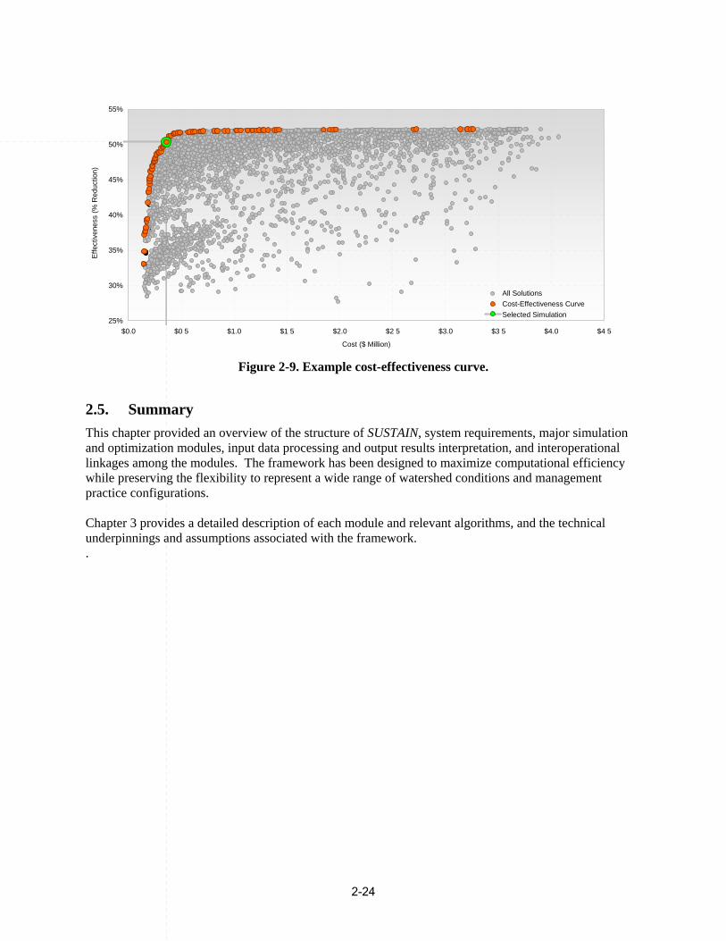
Effe

c tiv

enes

s (%

Red

uctio

n)

55%

50%

45%

40%

35%

30% All Solutions Cost-Effectiveness Curve Selected Simulation

25% $0.0 $0 5 $1.0 $1 5 $2.0 $2 5 $3.0 $3 5 $4.0 $4 5

Cost ( $ Million) Figure 2-9. Example cost-effectiveness curve.

2.5. Summary This chapter provided an overview of the structure of SUSTAIN, system requirements, major simulation and optimization modules, input data processing and output results interpreta tion, and interoperational linkages amo ng the modules. The framewor k has been designed to maximiz e computational efficiency while preserving the flexibility to represent a wide range of watershed conditions and management practice configurations. Chapter 3 provides a detailed description of each mo dule and relevant algorithms, and the technical underpinnings and assumptions associated w ith the framework. .

2-24

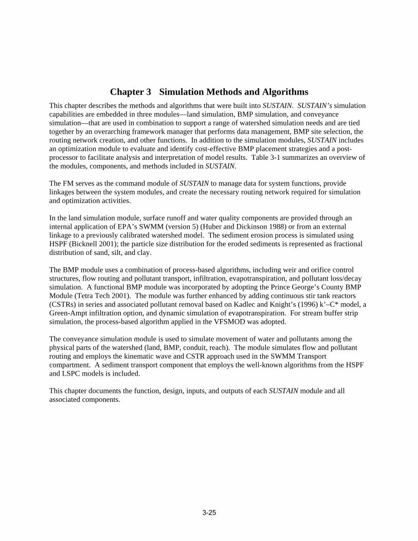
Chapter 3 Simulation Methods and Algorithms This chapter describes the methods and algorithms that were built into SUSTAIN. SUSTAIN’s simulation capabilities are embed ded in three modules—land simulation, BMP simulation, and conveyance simulat ion—that are used in combination to support a range of watershed simulation needs and are tied together by an overarching framework manager that performs data management, BMP site selection, the routing network creatio n, and other functions. In addition to the simulation modules, SUSTAIN includes an optimization module to evaluate and identify cost-effective BMP placement strategies and a post­processor to facilitate analysis and interpretation of mode l results. Table 3-1 summarizes an overview of the modules, components, and methods included i n SUSTAIN.

The FM serves as the command module of SUSTAIN to manage data for system functions, provide linkages between the system modules, and create the necessary routing network required for simulation and optimization activities.

In the land simulation module, surface runoff and water quality components are provided thro ugh an internal application of EPA’s SWMM (v ersion 5) (Huber and Dickinson 1988) or from an external linkage to a previously calibrated watershed model. The sediment erosion process is simulated using HSPF (Bicknell 2001); the particle size distribution for the eroded sediments is represented as fractional distribution of sand, silt, and clay.

The BMP module uses a combination of process-based algorithms, including weir and orifice control structures, flow routing and pollutant transport, infiltration, evapotranspiration, and pollutant loss/decay simulation. A functional BMP module was inc orporated by adopting the Prince George’s County BMP Module (Tetra Tech 2001). The module was further enhanced by addi ng continuous stir tank reactors (CSTRs) in series and associa ted pollutant removal based on Kadlec and Knight’s (1996) k’–C* model, a Green-Ampt infiltration option, and dynamic simula tion of evapotranspiration. For stream buffer strip simulation, the process-based algorithm applied in the VFSMOD was adopted.

The con eyance simulation module is used to v simulate movement of water and pollutants among the physical parts of the watershed (land, BMP, conduit, reach). The module simulates flow and pollutant routing and employs the kinematic wave and CSTR approach used in the SWMM Transport compartment. A sediment transport component that employs the well-known algorithms from the HSPF and LSPC models is included.

This chapter documents the function, design, inputs, and outputs of each SUSTAIN module and all associated components.

3-25

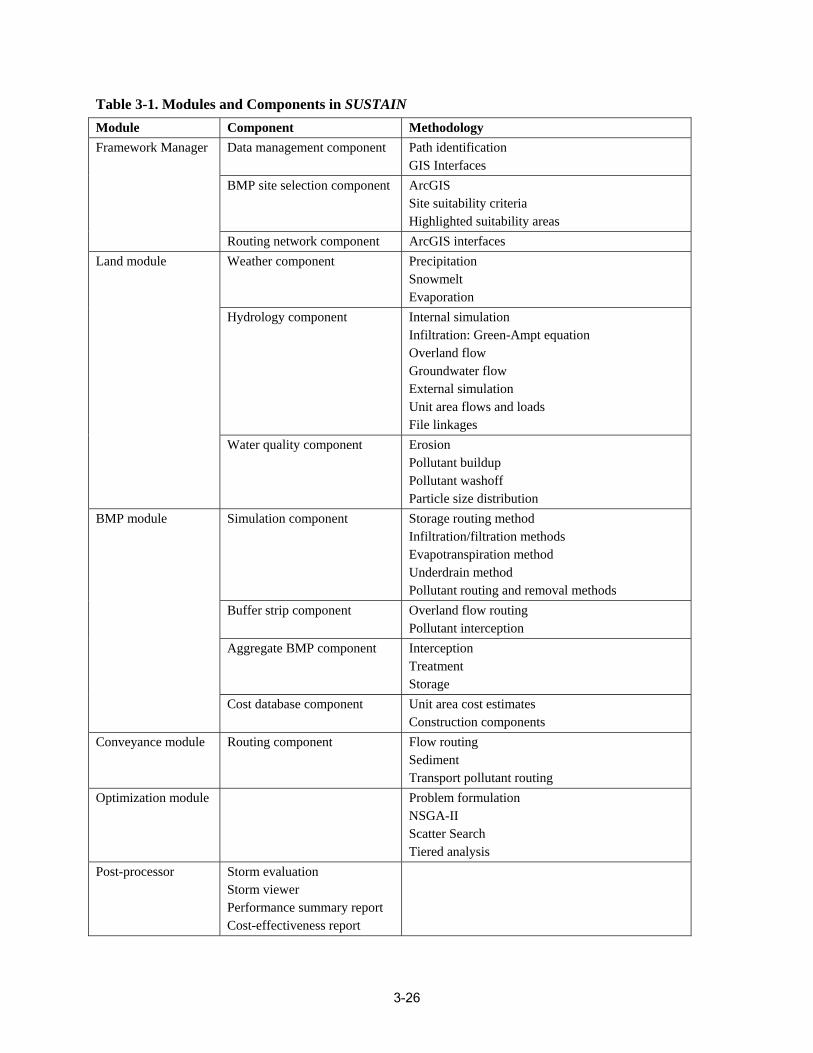
Table 3 1. Modules and Comp - onents in SUSTAIN Module Component Methodology Framework Manager Data management component Path identification

GIS Interfaces BMP site selection component ArcGIS

Site suitability criteria Highlighted suitability areas

Routing network component ArcGIS interfaces Land module Weather component Precipitation

Evaporation Snowmelt

H mydrology co ponent Internal simulation Infiltration: Green-Ampt equation Overland flow Groundwater flow External simulation Unit area flows and loads File linkages

Water quality component Erosion Pollutant buildup Pollutant washoff Particle size distribution

BMP module Simulation component Storage routing method Infiltration/filtration methods Evapotranspiration method Underdrain method Pollutant routing and removal methods

Buffer strip component Overland flow routing Pollutant interception

Aggregate BMP component Interception Treatment Storage

Cost database component Unit area cost estimates Construction components

Conveyance module Routing component Flow routing Sediment Transport pollutant routing

Optimization module Problem formulation NSGA-II Scatter Search Tiered analysis

Post-processor Storm evaluation Storm viewer Performance summary report Cost-effectiveness report

3-26

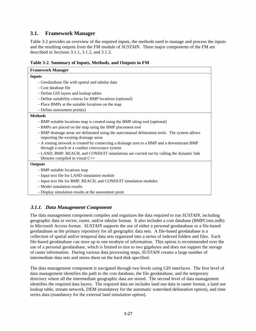
Table 3-2. Summary of Inputs, Methods, and Outputs in FM

anagFramework M er Inputs

− Geodat abase th spatial and tabular file wi data − Cost d atabase file − Defin e GIS la nd loo yers a bles kup ta − itabil Define su iteria fo ity cr P locati r BM optional) ons ( − MPs aPlace B t the suitable locations on th ap e m − e assess Defin nt(s ment poi )

Methods − BMP suitable l ons m ocati reated us ap is c he BMP siti ing t ng too l (option al) − Ps are placed on the map using the BMP placement tool BM − P drainage BM s are de area ted using linea uto/manual the a ation too deline he system allow ls. T s impo rting the existing drainage areas − ing netw A rout s creat ork i y connectin ed b g a drainage area to a BMP and ownstr a d eam BMP

h a reacthroug h or a conduit conveyance syste m − MP, LAND, B H, an REAC NDUIT si d CO lations are ca mu rried o ut by ca he dy lling t ic linam nk

es librari com piled i n visu al C++ Outputs

− BMP suitable l tions m oca ap − Inpu t text file for LAND si tion modulmula e − Input text file MP, R for B nd CO EACH, a NDU − el simulati Mod lts on resu

IT simulat es ion modul

− Display simulation results at the assessment point

3.1. Framework Manager Table 3-2 provides an overview of the required i nputs, the methods used to manage and process the inputs and the resulting outputs from the FM module of SUSTAIN. Three major com ponents of the FM are described in Sections 3.1.1, 3.1.2, and 3.1.3.

3.1.1. Data Management Component The data management component compiles and organizes the data required to run SUSTAIN, includin g geographic data in vector, raster, and/or tabular format. It also includes a cost database (BMPCosts.mdb) in Microsoft Access format. SUSTAIN supports the use of either a personal geodatabase or a file-based geodatabase as the primary repository for all geographic data sets. A file-based geodatabase is a collection of spati al and/or temporal data sets organized into a series of indexed folders and files. Each file-based geodatabase can store up to one terabyte of information. This option is recommended over the use of a personal geodatabase, which is limited in size to two gigabytes and does not support the storage of raster information. During various data processing steps, SUSTAIN creates a large number of intermediate data sets and stores them on the hard disk specified.

The data management component is navigated through two levels using GIS interfaces. The first level of data management identifies the path to the cost database, the file geodatabase, and the temporary directory where all the intermediate geographic data are stored. The second level of data management identifies the required data layers. The required data set includes land use data in raster format, a land use lookup table, stream network, DEM (mandatory for the automatic watershed delineation option), and time series data (mandatory for the external land simulation option).

3-27

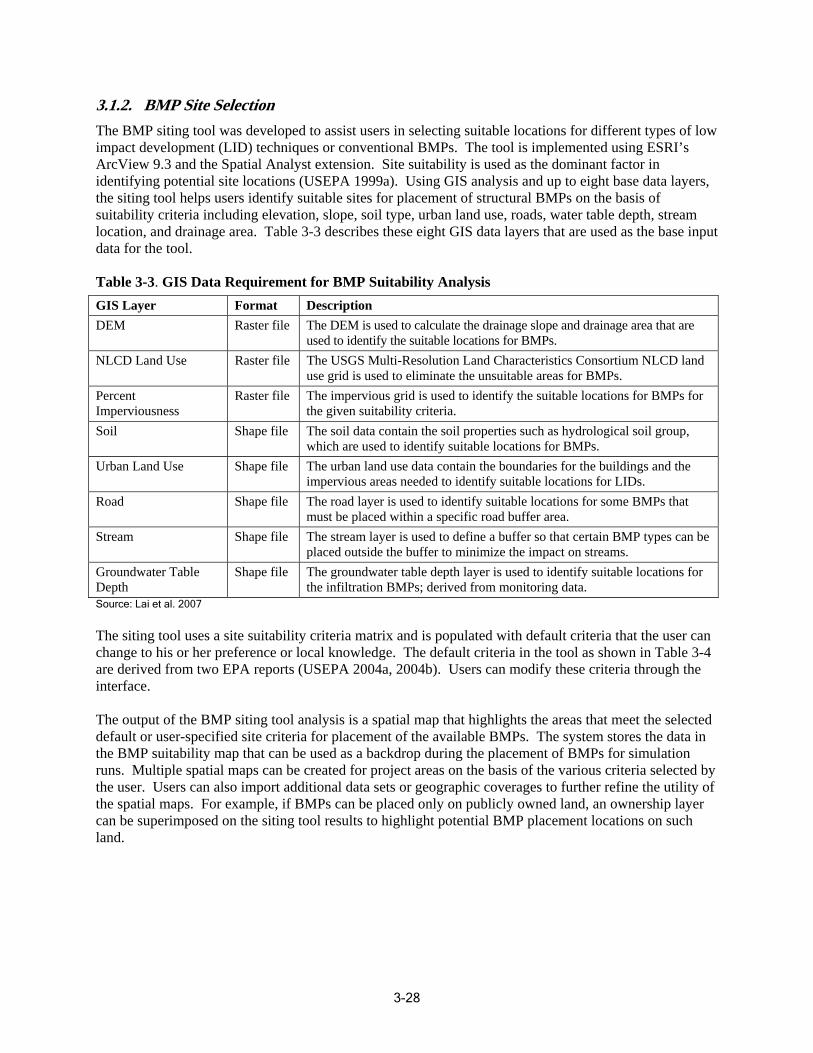
3.1.2. BMP Site Selection The BMP siting tool was dev eloped to ass ist users in selecting suitable locations for different types of low impact devel opment (LID) te chniques or conventional BMPs. The tool is implemented using ESRI’s ArcView 9.3 and the Spati al A nalyst ext ension. Site suitability is used as the dominant factor in identifying potential site locations (USEPA 1999a). Using GIS analysis and up to eight base data layers, the siting tool helps users identify suitable sites for placement of structural BMPs on the basis of suitability criteria including elevation, slope, soil type, urban land use, roads, water table depth, stream location, and d rainage area. Table 3-3 describes these eight GIS data layers that are used as the base input data for the tool.

Table 3-3. GIS Data Requirement for BMP Suitability Analysis GIS Layer Format ription Desc DEM Raster file DEM is used to calculate the drainage slope and drainage area that are

identify the suitable locations for BMPs. The used to

NLCD Land Use Raster file SGS Multi-Resolution Land Characteristics Consortium NLCD land d is used to eliminate the unsuitable areas for BMPs.

The U use gri

Percent Imperviousness

Raster file pervious grid is used to identify the suitable locations for BMPs for ven suitability criteria.

The im the gi

Soil Shape file The soil data contain the soil properties such as hydrological soil group, which are used to identify suitable locations for BMPs.

U arban L nd Use le Shape fi The urban land use data contain the boundaries for the buildings and the impervious areas needed to identify suitable locations for LIDs.

Road Shape file The road layer is used to identify suitable locations for some BMPs that must be placed within a specific road buffer area.

Stream Shape file The stream layer is used to define a buffer so that certain BMP types can be placed outside the buffer to minimize the impact on streams.

Groundwater Table Depth

Shape file The groundwater table depth layer is used to identify suitable locations for the infiltration BMPs; derived from monitoring data.

Source: Lai et al. 2007

The siting tool uses a site suitability criteria matrix and is populated with default criteria that the user can change to his or her preference or local knowledge. The default criteria in the tool as shown in Table 3-4 are derived from two EPA reports (USEPA 2004a, 2004b). Users can modify these criteria through the interface.

The output of the BMP siting tool analysis is a spatial map that highlights the areas that meet the selected default or user-specified site criteria for placement of the available BMPs. The system stores the data in the BMP suitability map that can be used as a backdrop during the placement of BMPs for simulation runs. Multiple spatial maps can be created for project areas on the basis of the various criteria selected by the user. Users can also import additional data sets or geographic coverages to further refine the utility of the spatial maps. For example, if BMPs can be placed only on publicly owned land, an ownership layer can be superimposed on the siting tool results to highlight potential BMP placement locations on such land.

3-28

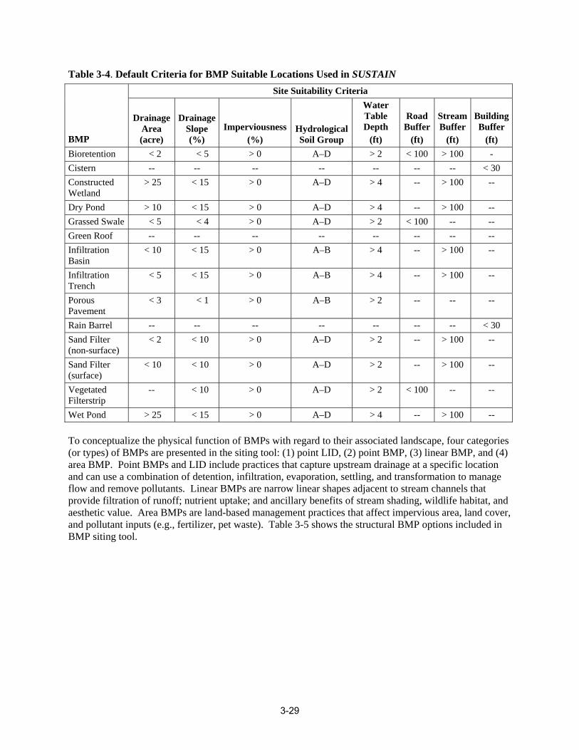
Table 3-4. Default Criter ia for BMP Suitable Locations Used in SUSTAIN

BMP

Site Suitability Criteria

Drainage Area (acre)

Drainage Slope (%)

Imperviousness (%)

Hydrological Soil Group

Water Table Depth

(ft)

Road Buffer

(ft)

Stream Buffer

(ft)

Bui Buffer

(ft)

lding

Bioretention < 2 < 5 > 0 A–D > 2 < 100 > 100 -Cistern -- -- -- -- -- -- -- < 30 Constructed Wetland

> 25 < 15 > 0 A–D > 4 -- > 100 --

Dry Pond > 10 < 15 > 0 A–D > 4 -- > 100 --Grassed Swale < 5 < 4 > 0 A–D > 2 < 100 -- --Green Roof -- -- -- -- -- -- -- --Infiltration Basin

< 10 < 15 > 0 A–B > 4 -- > 100 --

Infiltration rench T

< 5 < 15 > 0 A–B > 4 -- > 100 --

Porous Pavement

< 3 < 1 > 0 A–B > 2 -- -- --

Rain Barrel -- -­ -- -- -- -- -- < 30 Sand Filter (non-surface)

< 2 < 10 > 0 A–D > 2 -- > 100 --

Sand Filter (surface)

< 10 < 10 > 0 A–D > 2 -- > 100 --

Vegetated Filterstrip

-- < 10 > 0 A–D > 2 < 100 -- --

Wet Pond > 25 < 15 > 0 A–D > 4 -- > 100 --

To conceptualize the physical function of BMPs with regard to their associated landscape, four categories (or types) of BMPs are presented in the siting tool: (1) point LID, (2) point BMP, (3) linear BMP, and (4) area BMP. Point BMPs and LID include practices that capture upstream drainage at a specific location and can use a combination of detention, infiltration, evaporation, settling, and transformation to manage flow and remove pollutants. Linear BMPs are narrow linear shapes adjacent to stream channels that provide filtration of runoff; nutrient uptake; and ancillary benefits of stream shading, wildlife habitat, and aesthetic value. Area BMPs are land-based management practices that affect impervious area, land cover, and pollutant inputs (e.g., fertilizer, pet waste). Table 3-5 shows the structural BMP options included in BMP siting tool.

3-29

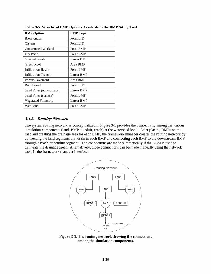
Table 3-5. Structural BMP Options Available in the BMP Siting Tool BMP Option BMP Type Bioretention Point LID Cistern Point LID Con structed Wetland Point BMP Dry Pond Point BMP Grassed Swale Linear BMP Green Roof rea BMP A Infiltration Basin oint BMP P Infiltration Trench ear BMP Lin Porous Pavement Area BMP Rain Barrel Point LID Sand Filter (non-surface) Linear BMP Sand Filter (surface) Point BMP Vegetated Filterstrip Linear BMP Wet Pond Point BMP

3.1.3. Routing Network The system rou ting network as conceptualized in Figure 3-1 provides the connectivity among the various sim ulation components (land, BMP, conduit, reach) at the watershed level. After placing BMPs on the map and creating the drainage area for each BMP, the framework manager creates the routing network by connecting the land segments that drain to each BMP and connecting each BMP to t he downstream BMP through a reach or conduit segment. The connections are made automatically if the DEM is used to delineate the drainage areas. Alternatively, those connect ions can be made manually using the network tools in the framework manager interface.

BMP

REACH

CONDUIT

LAND

REACH

LAND LAND

BMP BMP

Routing Network

Assessment Point

Figure 3-1. The routing network showing the connections among the simulation components.

3-30

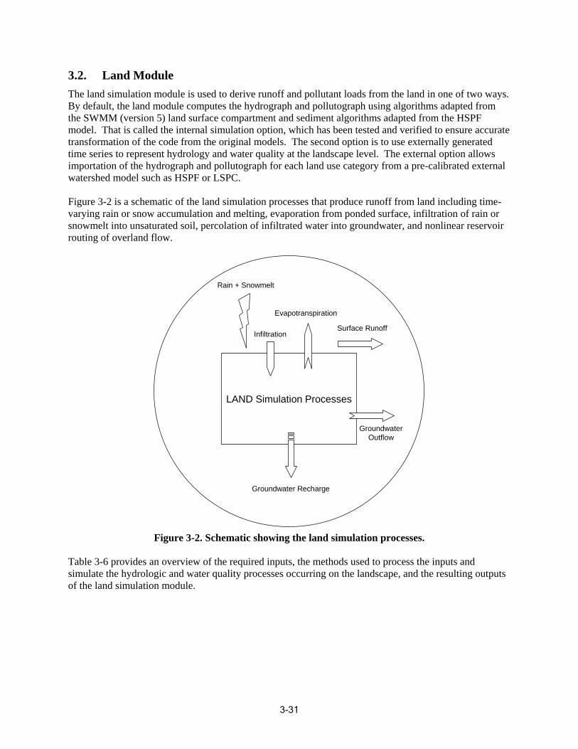
3.2. Land Module The land simulation module is used to derive runoff and pollutant loads from the land in one of two ways. By default, the land module computes the hydrograph and po llutograph using algorithms adapted from the SWMM (version 5) land surface compartment and sediment al gorithms adapted from the HSPF model. That is called the internal simulation op tion, whic h has been tested and verified to ensure accurate transformation of th e code from the o riginal models. The second option is to use ex ternally genera ted time series to represent hydrology and wa ter quality at the landscape level. The external option allows importatio n of the hydrograph and polluto graph for each land use category f rom a p re-calibrated ex ternal watershed m odel such as HSPF or LSPC.

a schematic of the land simulation proce ses that produce runoff from l and including tim e-Figure 3-2 is svarying rai n or snow accumulatio n and melting, evaporation from ponded surface, infiltration of rain or snowmelt into uns aturated soil, percolation of infiltrated water into groundwater, and nonlinear reservoir routing of overland flow.

LAND Simulatio rocesses n P

Rain + Snowmelt

Surface R f

Evapotranspiration

Infiltration unof

Groundwater Recharge

Groundwater Outflow

Figure 3-2. Schematic showing the land simulation processes.

Table 3-6 provides an overview of the required inputs, the methods used to process the inputs and simulate the hydrologic and water quality processes occurring on the landscape, and the resulting outputs of the land simulation module.

3-31

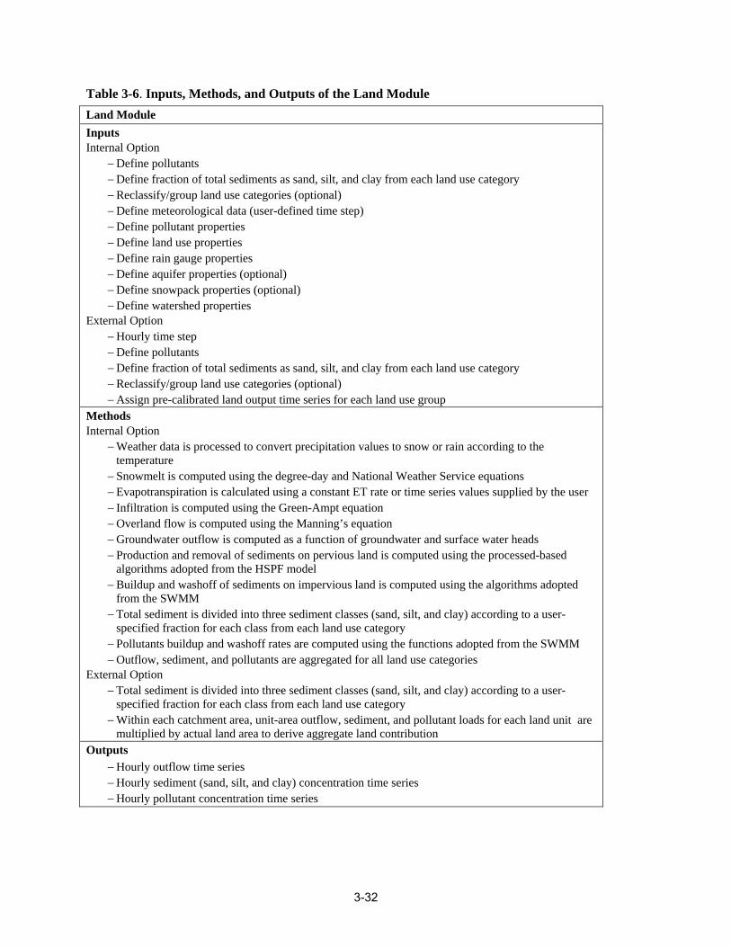
Table 3-6. Inputs, Methods, and Outputs of the Land Module Land Module

Inputs Internal Option

− Define pollutants − Define fraction of total sediments as sand, silt, and clay from each land use category − Reclassify/group land use categories (optional) − Define meteorological data (user-defined time step) − Define pollutant properties − Define land use properties − Define rain gauge properties − Define aquifer properties (optional) − Define snowpack properties (optional) − Define watershed properties

External Option − Hourly time step − Define pollutants − diments as sand, silt, and clay from each land use category Define fraction of total se − nd use categories (optional) Reclassify/group la − Assign pre-calibrated land output time series for each land use group

Methods Internal Option

− Weath er data is processed to convert precipitation values to snow or rain according to the te mperature − Sn r Service equations owmelt is computed using the degree-day and National Weathe − Ev u e series values supplied by the user apotranspiration is calc lated using a constant ET rate or tim − In filtration is computed using the Green-Ampt equ ation − Ov erland flow is computed using the Manning’s equation − Groundwat er outflow is computed as a function of groundwater and surface water heads − Production and removal of sediments on pervious land is computed using the processed-based

algorithms adopted from the HSPF model − Buildup and washoff of sediments on impervious land is computed using the algorithms adopted

from the SWMM − Total sediment is divided into three sediment classes (sand, silt, and clay) according to a user­

ecified fraction for each class from each land use category sp − oP llutants buildup and washoff rates are computed using the functions adopted from the SWMM − Ou and use categories tflow, sediment, and pollutants are aggregated for all l

xternal E Option − To tal sediment is divided into three sediment c lasses (sand, silt, and clay) according to a user­sp eci fied fraction for each class from each land use category − W ithin each catchment area, unit-area outflow, sed iment, and pollutant loads for each land unit are mu ltiplied by actual land area to derive aggregate land contribution

Outputs − Hourly outflow time series − Hourly sediment (sand, silt, an tration time series d clay) concen − Hourly pollutant concen ation time series tr

3-32

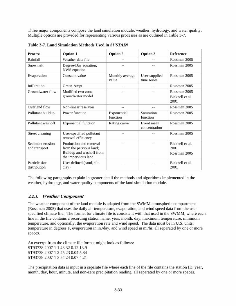
Three major components compose the land simulation module: weather, hydrology, and water quality. Multiple options are provided for representing various processes as are outlined in Table 3-7.

Table 3-7. Land Simulation Methods Used in SUSTAIN

Process Option 1 Option 2 Option 3 Reference Rainfall Weather data fil e -- -- Rossman 2005 Snowme lt ion; Degree-Day equat

NWS equation -- -- Rossman 2005

Evaporation Constant value Monthly average value

User-supplied time series

Rossman 2005

Infiltration Green-Ampt -- -- Rossman 2005 Groundwater flow Modified two-zone

groundwater model -- -- Rossman 2005

Bicknell et al. 2001

O flow verland Non-linear reservoir -- -- Rossman 2005 Pollutant buildup Power function Exponential

function Saturation function

Rossman 2005

Pollutant washoff Exponential function Rating curve Event mean concentration

Rossman 2005

Street cleaning User-specified pollutant removal efficiency

-- -- Rossman 2005

S erosion an t

ediment d transpor

Production and from the pervious land; Buildup and washoff from

removal

the impervious land

-- -- Bicknell et al. 2001 Rossman 2005

Particle size distribution

User defined (sand, silt, clay)

-- -- Bicknell et al. 2001

The following paragraphs explain in greater detail the methods and algorithms implemented in the weather, hydrology, and water quality components of the land simulation module.

3.2.1. Weather Component The weather component of the land module is adapted from the SWMM atmospheric compartment (Rossman 2005) that uses the daily air temperature, evaporation, and wind speed data from the user-specified climate file. The format for climate file is consistent with that used in the SWMM, where each line in the file contains a recording station name, year, month, day, maximum temperature, minimum temperature, and optionally, the evaporation rate and wind speed. The data must be in U.S. units: temperature in degrees F, evaporation in in./day, and wind speed in mi/hr, all separated by one or more spaces.

An excerpt from the climate file format might look as follows: ST93738 2007 1 1 43 32 0.12 13.9 ST93738 2007 1 2 45 23 0.04 5.84 ST93738 2007 1 3 54 24 0.07 4.21

The precipitation data is input in a separate file where each line of the file contains the station ID, year, month, day, hour, minute, and non-zero precipitation reading, all separated by one or more spaces.

3-33

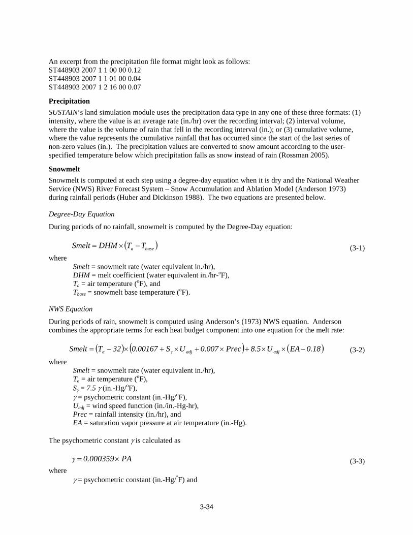
An excerpt from the precipitation file format might look as follows: ST448903 2007 1 1 00 00 0.12 ST448903 2007 1 1 01 00 0.04 ST448903 2007 1 2 16 00 0.07

Precipitation SUSTAIN’s land simulation module uses the precipitation data type in any one of these three formats: (1) intensity, where the value is an average rate (in./hr) over the recording interval; (2) interval volume, where the value is the volume of rain that fell in the recording interval (in.); or (3) cumulative volume, where the value represents the cumulative rainfall that has occurred since the start of the last series o f non-zero values (in.). The precipitation values are converted to snow amount according to the user-specified temperature below which precipitation falls as snow instead of rain (Rossman 2005).

Snowmelt Snowmelt is computed at each s tep using a degree-day equation when it is dry and the National Weather Service (NWS) River Forecast System – Snow Accumulation and Ablation Model (Anderson 1973) during rainfall periods (Huber and Dickinson 1988). The two equ ations are presented below.

Degree-Day Equation

During periods of no rainfall, snowmelt is computed by the Degree-Day equation:

Smelt = DHM ×(Ta −Tbase ) (3-1) where

Smelt = snowmelt rate (water equivalent in./hr), DHM = melt coefficient (water equivalent in./hr-oF), Ta = air temperature (oF), and Tbase = snowmelt base temperature (oF).

NWS Equation

During periods of rain, snowmelt is computed using Anderson’s (1973) NWS equation. Anderson combines the appropriate terms for each heat budget component into one equation for the melt rate:

Smelt = (Ta − 32)× (0.00167 + S γ ×U adj + 0.007 × Prec)+ 8.5 ×U adj × (EA − 0.18) (3-2) where

Smelt = snowmelt rate (water equivalent in./hr), Ta = air temperature (oF), Sγ = 7.5 γ (in.-Hg/oF), γ = psychometric constant (in.-Hg/oF), Uadj = wind speed function (in./in.-Hg-hr), Prec = rainfall intensity (in./hr), and EA = saturation vapor pressure at air temperature (in.-Hg).

The psych ometric constant γ is calculated as

γ = 0.000359 × PA (3-3) where

γ = psychometric constant (in.-Hg/ °F) and

3-34

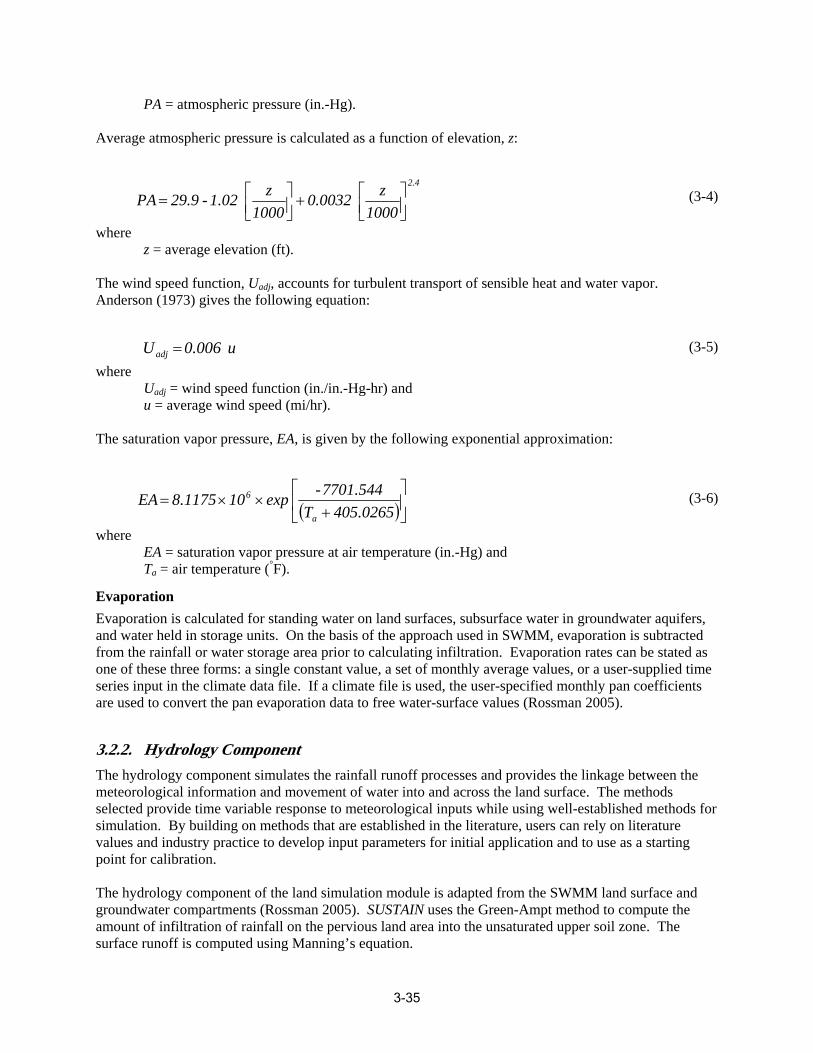
PA = atmospheric pressure (in.-Hg).

Average atmospheric pressure is calcu lated as a function of elevation, z:

⎡ z ⎤ ⎡ z ⎤2.4

(3-4)PA = 29.9 - 1.02 0.0032⎢⎣1000 ⎥⎦+ ⎢⎣1000 ⎥⎦

where z = average elevation (ft).

The wind speed function, Uadj, accounts for turbulent transport of sensible heat and water vapor. Anderson (1973) gives the following eq uation:

Uadj = 0.006 u (3-5)

where Uadj = wind speed function (in./in.-Hg-hr) and u = average wind speed (mi/hr).

The saturation vapor pres sure, EA, is given by the fol lowing exponen tial approximatio n:

6 ⎡ -7701.544 ⎤EA = 8.1175 ×10 × exp (3-6)⎢ ⎥

⎣(Ta + 405.0265)⎦ where

EA = saturation vapor pressure at air te mperature (in.-Hg) and Ta = air temperature ( °F).

Evaporation Evaporation is calculated for standing water on land surfaces, subsurface water in groundwater aquifers, and water held in storage units. On the basis of the approach used in SWMM, evaporation is subtracted from the rainfall or water storage area prior to calculating infiltration. Evaporation rates can be stated as one of these three forms: a single constant value, a set of monthly average values, or a user-suppli ed time series input in the climate data file. If a climate file is used, the user-specified monthly pan coefficients are used to convert the pan evaporation data to free water-surf ace values (Rossman 2005).

3.2.2. Hydrology Component The hydrology component simulates the rainfall runoff processes and provides the linkage between the meteorological information and movement of water into and across the land surface. The methods selected provide time variable response to meteorological inputs while using well-established metho ds for simulation. By building on methods that are established in the literature, users can rely on literature values and industry practice to develop input parameters for initial application and to use as a starting point for calibration.

The hydrology compon ent of the land simulation module is adapted from the SWMM land surface and groundwater compartments (Rossman 2005). SUSTAIN uses the Green-Ampt method to compute the amount of infiltration of rainfall on the pervious land area into the unsaturated upper soil zone. The surface runoff is computed using Manning’s eq uation.

3-35

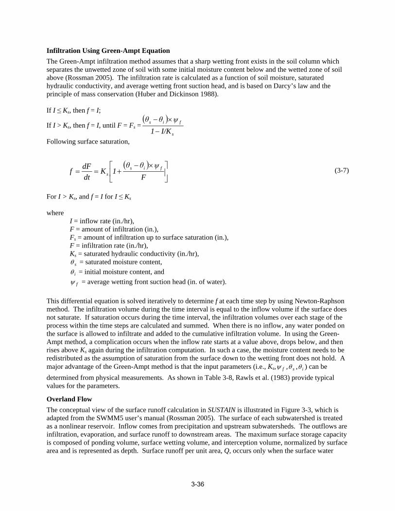
Infiltration Using Green-Ampt Equation The Green-Ampt infiltration method assumes that a sharp wetting front exists in the soil column which separates the unwetted zone of soil with some initial moisture content below and the wetted zone of soil above (Rossman 2005). The infiltration rate is calculated as a function of soil moisture, saturated hydraulic conductivity, and average wetting front suction head, and is based on Darcy’s law and the principle of mass conservation (Huber and Dickinson 1988).

If I ≤ Ks, then f = I;

If I > Ks, then f = I, until F = Fs =(

θs − θi ×ψ f

1 − I/K s

)

Following surface saturation,

dF ⎡ (θs − θi )×ψ f ⎤

f = = K 1 + (3-7)s ⎢ ⎥dt F⎣ ⎦

For I > Ks, and f = I for I ≤ Ks

where I = inflow rate (in./hr),F = amount of infiltration (in.),

Fs = amount of infiltration up to surface saturation (in.), F = infiltration rate (in./hr),Ks = saturated hydraulic conductivity (in./hr), θ s = saturated moisture content, θ i = initial moisture content, and ψ f = average wetting front suction head (in. of water).

This differential equation is solved iteratively to determine f at each time step by using Newton-Raphson method. The infiltration volume during the t ime interval is equal to the inflow volume if the surface does not saturate. If saturation occurs during the time interval, the infiltration volumes over each stage of the process within the time steps are calculated and summed. When there is no inflow, any water ponded on the surface is allowed to infiltrate and added to the cumulative infiltration volume. In using the Green-Ampt method, a complication occurs when the inflow rate starts at a value above, drops below, and the n rises above Ks again during the infiltration computation. In such a case, the moisture content needs to be redistributed as the assumption of saturation from the surface down to the wetting front does not hol d. A major advantage of the Green-Ampt method is that the input parameters (i.e., Ks,ψ f ,θ s ,θ i ) can be determined from physical measurements. As shown in Table 3-8, Rawls et al. (1983) provide typical values for the parameters.

Overland Flow The conceptual view of the surface runoff calculation in SUSTAIN is illustrated in Figure 3-3, which is adapted from the SWMM5 user’s manual (Rossman 2005). The surface of each subwatershed is treated as a nonlinear reservoir. Inflow comes from precipitation and upstream subwatersheds. The outflows are infiltration, evaporation, and surface runoff to downstream areas. The maximum surface storage capacity is composed of ponding volume, surface wetting volume, and interception volume, normalized by surface area and is represented as depth. Surface runoff per unit area, Q, occurs only when the surface wate r

3-36

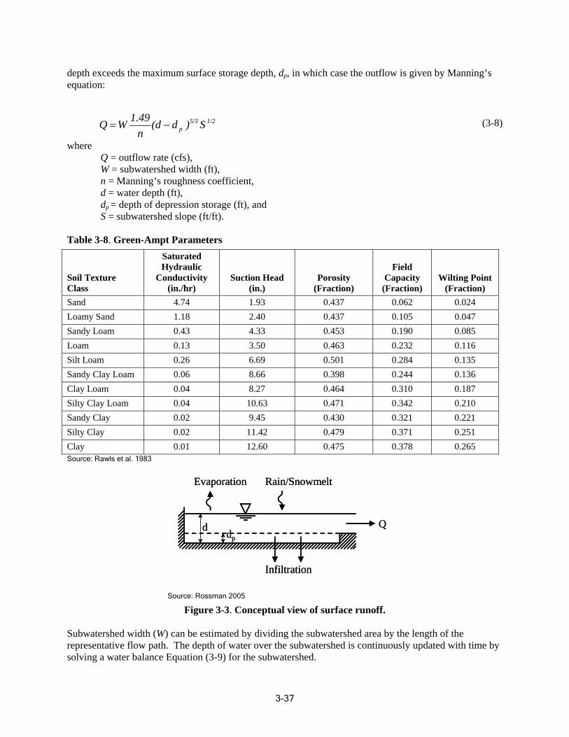
depth exceeds the maximum surface storage depth, dp, in which case the outflow is given by Manning’s equation:

1.49 5/3 1/2Q = W (d − d p ) S (3-8)

n where

Q = outflow rate (cfs), W = subwatershed width (ft), n = Manning’s roughness coefficient, d = water depth (ft), dp = depth of depression storage (ft), and S = subwatershed slope (ft/ft).

Table 3-8. Green-Ampt Parameters

Soil Texture Class

Saturated Hydraulic

Conductivity (in./hr)

Suction Head (in.)

Porosity (Fraction)

Field Capacity

(Fraction) Wilting Point

(Fraction) Sand 4.74 1.93 0.437 0.062 0.024 Loamy Sand 1.18 2.40 0.437 0.105 0.047 Sandy Loam 0.43 4.33 0.453 0.190 0.085 Loam 0.13 3.50 0.463 0.232 0.116 Silt Loam 0.26 6.69 0.501 0.284 0.135 Sandy Clay Loam 0.06 8.66 0.398 0.244 0.136 Clay Loam 0.04 8.27 0.464 0.310 0.187 Silty Clay Loam 0.04 10.63 0.471 0.342 0.210 Sandy Clay 0.02 9.45 0.430 0.321 0.221 Silty Clay 0.02 11.42 0.479 0.371 0.251 Clay 0.01 12.60 0.475 0.378 0.265

Source: Rawls et al. 1983

EEvvapapoorratationion RRaiain/Sn/Snnowowmmeeltlt

dpd Q

dp d Q

InfiltrationInfiltration

Source: Rossman 2005

Figure 3-3. Conceptual view of surface runoff.

Subwatershed width (W) can be estimated by dividing the subwatershed area by the length of the representative flow path. The depth of water over the subwatershed is continuously updated with time by solving a water balance Equation (3-9) for the subwatershed.

3-37

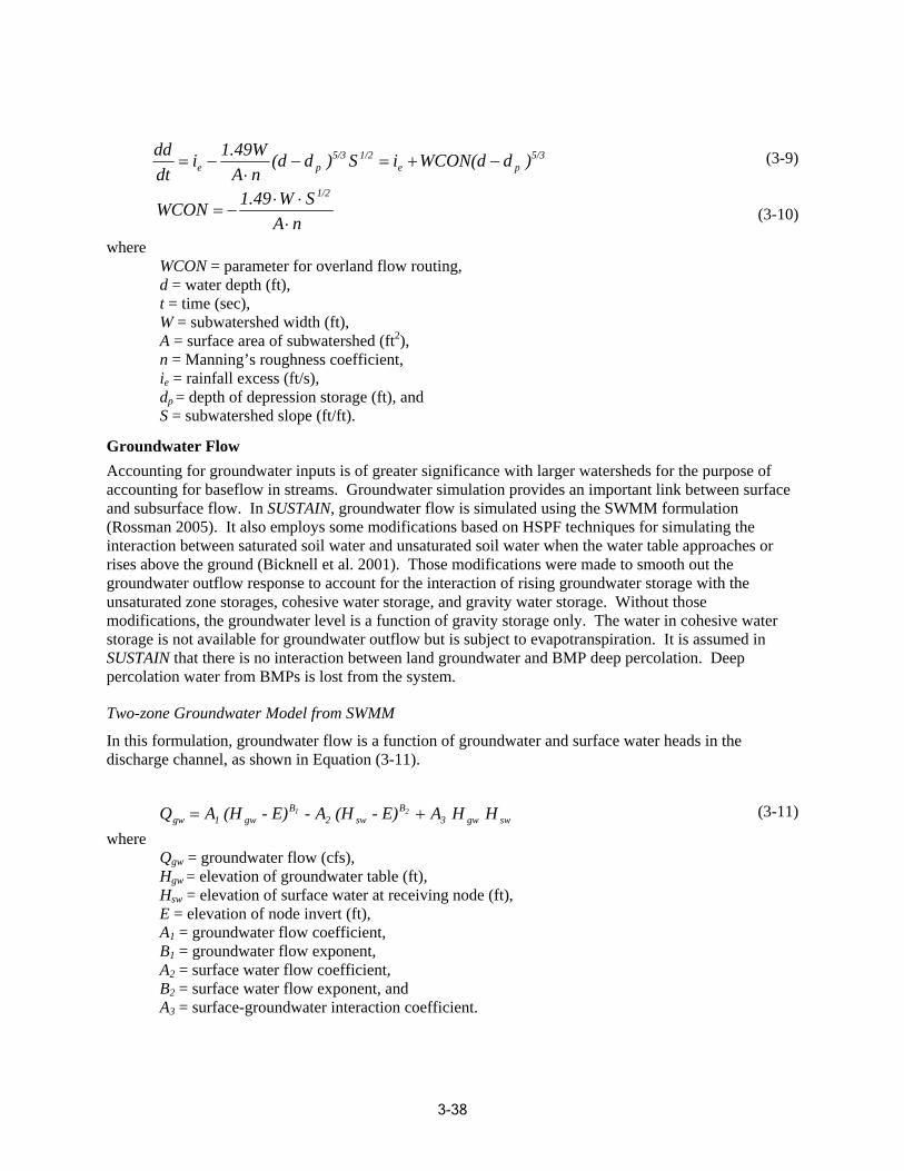
dd 1.49W 5/3 1/2 5/3= i − (d − d ) S = i +WCON(d − d ) (3-9)

e p e pdt A ⋅ n

1/21.49 ⋅W ⋅ SWCON = − (3-10)A ⋅ n

where WCON = parameter for overland flow routing,

d = water depth (ft), t = time (sec),

W = subwatershed width (ft), A = surface area of subwatershed (ft2), n = Manning’s roughness coefficient, ie = rainfall excess (ft/s), dp = depth of depression storage (ft), and S = subwatershed slope (ft/ft).

Groundwater Flow Accounting for groundwater inputs is of greater significance with larger watersheds for the purpose of accounting for baseflow in streams. Groundwater simulation provides an important lin k between surface and sub su rface flow. In SUSTAIN, groundwater flow is simulated using the SWMM formulation (Rossman 2005). It also employs some modifications based on HSPF techniques for simulating the interaction between saturated soil water and unsaturated soil water when the water tab le approaches or rises above the ground (Bicknell et al. 2001). Those modifications were made to smo oth out the groundwater outflow response to account for the interaction of rising groundwater storage with the unsaturated zone s torages, cohesive water storage, and gravity water storage. Without those modifications, the groundwater level is a function of gravity storage only. The water in cohesive water storage is not available for groundwater outflow but is subject to evapotranspiration. It is assumed in SUSTAIN that there is no interaction between land groundwater and BMP deep percolation. Deep percolation water from BMPs is lost from the system.

Two-zone Groundwater Model from SWMM

In this formu lation, groundwater flow is a function of groundwater and surface water heads in the discharge channel, as shown in Equation (3-11).

1 2Qgw = A (H gw - E)B - A (H sw - E)B + A3 H gw H sw (3-11)

1 2

where Qgw = groundwater flow (cfs), Hgw = elevation of groundwater table (ft), Hsw = elevation of surface water at receiving node (ft), E = elevation of node invert (ft), A1 = groundwater flow coefficient, B1 = groundwater flow exponent, A2 = surface water flow coefficient, B2 = surface water flow exponent, and A3 = surface-groundwater interaction coefficient.

3-38

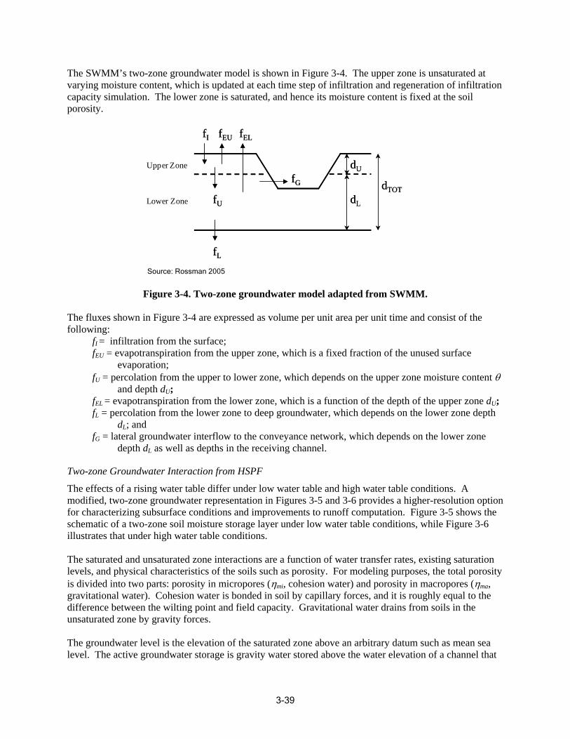
The SWMM’s two-zone groundwater model is shown in Figure 3-4. The upper zone is unsaturated at varying moisture content, which is updated at each time step of infiltration and regeneration of infiltration capacity simulation. The lower zone is saturated, and hence its moisture content is fixed at the soil porosity.

ffII ff fEUEU fELEL

dU

fU

fG

dL

dTOT

dU

fU

fG

dL

dTOT

Upper Zone

Lower Zone

ffLL

Source: Rossman 2005

Figure 3-4. Two-zone groundwater model adapted from SWMM.

The fluxes shown in Figure 3-4 are expressed as volume per unit area per unit time and consist of the following:

fI = infiltration from the surface; fEU = evapotranspiration from the upper zone, which is a fixed fraction of the unused surface

evaporation; fU = percolation from the upper to lower zone, which depends on the upper zone moisture content θ

and depth dU; fEL = evapotranspiration from the lower zone, which is a function of the depth of the upper zone dU; fL = percolation from the lower zone to deep groundwater, which depends on the lower zone depth

dL; and fG = lateral groundwater interflow to the conveyance network, which depends on the lower zone

depth dL as well as depths in the receiving channel.

Two-zone Groundwater Interaction from HSPF

The effects of a rising water table differ under low water table and high water table conditions. A modified, two-zone groundwater representation in Figures 3-5 and 3-6 provides a higher-resolution option for characterizing subsurface conditions and improvements to runoff computation. Figure 3-5 shows the schematic of a two-zone soil moisture storage layer under low water table conditions, while Figure 3-6 illustrates that under high water table conditions.

The saturated and unsaturated zone interactions are a function of water transfer rates, existing saturation levels, and physical characteristics of the soils such as porosity. For modeling purposes, the total porosity is divided into two parts: porosity in micropores (ηmi, cohesion water) and porosity in macropores (ηma, gravitational water). Cohesion water is bonded in soil by capillary forces, and it is roughly equal to the difference between the wilting point and field capacity. Gravitational water drains from soils in the unsaturated zone by gravity forces.

The groundw a ter level is the elevation of the saturated zone above an arbitrary datum such a s mean sealevel. The active groundwater storage is gravity water stored above the water elevation of a channel that

3-39

is within or adjacent to the land. A lower elevation is the maximum depth where soil moisture varies seasonally due to evapotranspiration.

When the groundwater elevation is below the lower elevation (within the saturated Zone 1 as shown in Figure 3-5), there is no interaction between the saturated and the unsaturated zones. Groundwater elevation in this zone is computed as a function of the groundwater storage and the total porosity (the sum of macropores and micropores).

ηηηηmimi mamaLaLanndd SuSurfacerface

LoLowweerr

2 EEvvapapototraransnspiratpiratiioonn

ZO

ZO

NE

NE

2

DepDeptthh

ONN

EE 11

HHgwgw

HHetet

HHchch SSttororageage

ZO

Z DatDatuumm

AAcctitiveve GGrroouundndwawateterr

Source: Bicknell et al. 2001

Figure 3-5. Two-zone soil moisture storage under low water table condition.

The groundwater elevation in this zone is calculated as:

SgwH gw = (3-12)

(η + η )mi ma

where Hgw = groundwater elevation (ft), Sgw = total groundwater storage (ft), ηmi = soil porosity in micropores (large pores for cohesive water), and ηma = soil porosity in macropores (large pores for gravitational water).

When the groundwater elevation reaches the higher elevation (within the unsaturated Zone 2 as shown in Figure 3-6), the groundwater storage starts interacting with the upper zone storages. Rising groundwater that occupies micropores is reassigned to the upper zone cohesive water storage. Groundwater storage shares macropores with the upper zone gravity water storage and is subject to evapotranspiration. Changes in groundwater storage are distributed between upper zone storages and groundwater storage, according to their relative saturation levels. Groundwater elevation in this zone is a function of upper zone water in macropores and groundwater storages and is calculated as:

H + [S + (S − S )]et uz gw lzHgw = (3-13)

ηma

where Het = elevation at the maximum depth due to seasonal evapotranspiration (ft), Sgw = total groundwater storage (ft), including all water in the lower saturated zone and in

macropores of the upper zone saturated soil,

3-40

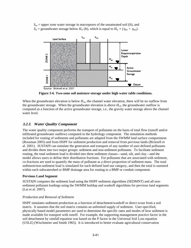
Suz = upper zone water storage in macropores of the unsaturated soil (ft), and Slz = groundwater storage below Het (ft), which is equal to Het × (ηmi + ηma).

ηηηηmimi mamaLaLand Snd Suurfarfaccee

ZO

ZO

NNEE

22

HHgwgw

HHetet ActiveActive

LoLowerwer EvEvaappototrraannsspipirraattiioonn DeptDepthh

GroGrouunnddwaterwater

1 StStoorrageage

ZO

ZO

NNEE

1

HHchch

DatDatuumm

Source: Bicknell et al. 2001

Figure 3-6. Two-zone soil moisture storage under high water table conditions.

When the groundwater elevation is below Hch, the channel water elevation, there will be no outflow from the groundwater storage. When the groundwater elevation is above Hch, the groundwater outflow is computed as a function of the active groundwater storage, i.e., the gravity water storage above the channel water level.

3.2.3. Water Quality Component The water quality component performs the transport of pollutants on the basis of total flow (runoff and/or infiltrated groundwater outflow) computed in the hydrology component. The simulation methods included for routing of sediments and pollutants are adapted from the SWMM land surface compartment (Rossman 2005) and from HSPF for sediment production and removal from pervious lands (Bicknell et al. 2001). SUSTAIN can simulate the generation and transport of any number of user-defined pollutants and divides them into two major groups: sediment and non-sediment pollutants. To facilitate sediment routing, the total sediment load is divided into three sediment classes—sand, silt, and clay—and the model allows users to define their distribution fractions. For pollutants that are associated with sediment, co-fractions are used to quantify the mass of pollutant as a direct proportion of sediment mass. The total sediment/non-sediment load is simulated for each defined land use category, and then the total is summed within each subwatershed or BMP drainage area for routing to a BMP or conduit component.

Pervious Land Segment SUSTAIN computes the sediment load using the HSPF sediment algorithms (SEDMNT) and all non-sediment pollutant loadings using the SWMM buildup and washoff algorithms for pervious land segments (Lai et al. 2007).

Production and Removal of Sediment

HSPF simulates sediment production as a function of detachment/washoff or direct scour from a soil matrix. It assumes that the soil matrix contains an unlimited supply of sediment. User-specified, physically based model parameters are used to determine the specific rates and modes of how sediment is made available for transport with runoff. For example, the supporting management practice factor in the soil detachment by rainfall equation was based on the P factor in the Universal Soil Loss equation (USLE) (Wischmeier and Smith 1965). It is introduced to better evaluate agricultural conservation

3-41

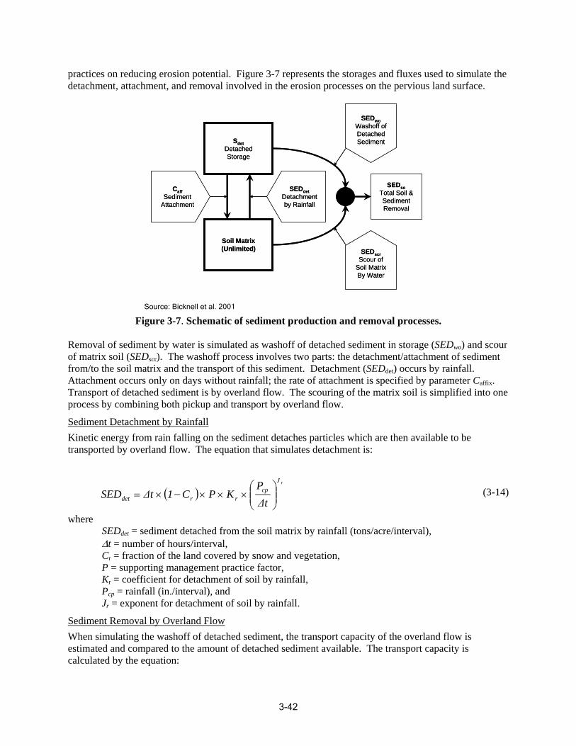
practices on reducing erosion potential. Figure 3-7 represents the storages and fluxes used to simulate the detachment, attachment, and removal involved in the erosion processes on the pervious land surface.

SEDwoWashoffDetache

ofd

S ntedime

St

EDdetachment Rainfall

Deby

CaffSedime

Attachm

SED

SedimentRemoval

ntent

SEDscrScour of

Soil MatrixBy Water

Total S

Soil Matrix(Unlimited)

SdetDetachedStorage

SEDwo Washoff Detache

of d

S ntedime

S t

EDdet achment Rainfall

De by

Caff Sedime

Attachm

SED

Sediment Removal

Total Snt ent

Soil Matrix (Unlimited) SEDscr

Scour of Soil Matrix By Water

Sdet Detached Storage

soso oiloil &&

Source: Bicknell et al. 2001

Figure 3-7. Schematic of sediment production and removal processes.

Removal of sediment by water is simulated as washoff of detached sediment in storage (SEDwo) and scour of matrix soil (SEDscr). The washoff process involves two parts: the detachment/attachment of sediment from/to the soil matrix and the transport of this sediment. Detachment (SEDdet) occurs by rainfall. Attachment occurs only on days without rainfall; the rate of attachment is specified by parameter Caffix. Transport of detached sediment is by overland flow. The scouring of the matrix soil is simplified into one process by combining both pickup and transport by overland flow.

Sediment Detachment by Rainfall Kinetic energy from rain falling on the sediment detaches particles which are then available to be transported by overland flow. The equation that simulates detachment is:

⎛ Pcp ⎞

J r

SED = ∆t × (1 − C )× P × K × ⎜⎜ ⎟⎟ (3-14)det r r ∆t⎝ ⎠

where SEDdet = sediment detached from the soil matrix by rainfall (tons/acre/interval), ∆t = number of hours/interval, Cr = fraction of the land covered by snow and vegetation, P = supporting management practice factor, Kr = coefficient for detachment of soil by rainfall, Pcp = rainfall (in./interval), and Jr = exponent for detachment of soil by rainfall.

Sediment Removal by Overland Flow When simulating the washoff of detached sediment, the transport capacity of the overland flow is estimated and compared to the amount of detached sediment available. The transport capacity is calculated by the equation:

3-42

⎛ qs ⎞Js

(3-15)SED = ∆t × K × ⎜ ⎟cap s ⎝ ∆t ⎠

where

SEDcap = transport capacity of detached sedim ent in overland flow (tons/acre/interval), ∆t = number of hours/int rval, e Ks = coefficien t for detached sediment by overland flow, qs = overland flow (in./interval), and Js = exponent for detached sediment by overland flow.

When SEDcap is more than the amount of detached sediment in storage ( Sdet), the flow washes off all th e detached sediment st orage, and SEDwo becomes equal to Sdet. However, when SEDcap is less than Sdet, the situation is transpo rt limiting, so SEDwo is equal to SEDcap.

Direct detachment and transport of the soil matrix by scouring (e.g., gullying) is sim ulated with t he equation:

⎛ qs ⎞J g

SEDscr = ∆t × K g × ⎜ ⎟ (3-16) ⎝ ∆t ⎠

where SEDscr = scour of matrix soil (tons/acre/interval), ∆t = number of hours/interval, Kg = coefficient for scour of the matrix soil, qs = surface flo w (in./interval), and

Jg = exponent for scour of the matrix soil.

The sum of the two fluxes, SEDwo and SEDscr, represents the total sediment outflow (SEDso) from the land segment.

Re-attach ment of Deta ched Sediment Sedimen t attachme nt to the soil matrix is simulated by changes in SEDdet. Because the soil matrix is considered to be unlimi ted, no addition to the so il matrix is necessary when this occurs. Sdet is diminis hed at the start of each day following a da y without preci pitation. This decrease is cal culated by multiply ingSdet by (1.0 - C affix), where Caffix is the fraction by which detached sediment storage de creases each day a s a result of soil compaction. This fraction is a calibration p aramete r.

Pervious Land Sediment Input Parameters Table 3-9 shows the recomm ended ranges of input parameters for simulating the pervious land segment. The minimum and ma ximum ranges given in Table 3-9 are for the numerical stability of the model. The actual values fall withi n those ranges and are typically defined by calibration and user experience. Additional HSPF parameterization guidance is available as part of the Better Assessment Scie nce Integrating Point and Nonpoint Sources (BASINS) technical note series at http://www.epa.gov/waterscience/basins/docs/tecnote8.pdf (USEPA 2006).

3-43

Table 3-9. List of Sediment Input Parameters for Pervious Land Parameters Default Value Min. Value Max. Value Units P 1.0 0.001 1.0 none Kr 0.0 0.0 none -Jr none none none -Caffix 0.0 0.0 1.0 per day Cr 0.0 0.0 1.0 none Ks 0.0 0.0 none -Js none none none -Kg 0.0 0.0 none -Jg none none none -Source: Bicknell et al. 2001

Pervious Land Sediment Erosion Calibration The erosion process on pervious land areas is represented as the net result of detachment of soil particles by raindrop impact on the land surface and subsequent transport of the fine particles by overland flow. The primary sediment erosion calibration parameters are as follows:

Kr = coefficient in soil detachment equation (pervious area) Ks = coefficient in sediment washoff equation (pervious area)

Although a number of additional parameters are involved in sediment erosion calibration, such as those related to vegetation cover, agricultural practices, rainfall, and overland flow intensity, Kr and Ks are the primary parameters controlling sediment loading rates. Kr is usually estimated as equal to the erodibility factor, K, in the USLE (Wischmeier and Smith 1965) and then is adjusted in calibra tion. Ks is primarily evaluated through calibration and past experience.

While Table 3-9 presents possible parameter ranges to e nsure model stability, Table 3-10 lists the sediment parameters along with typical and possible minimum an d maximum ranges of values based on application experience over the past 20 years. In addition, the HSPFParm database (USEPA 1999) provides calibrated parameter values for numerous watersheds across the United States. Additional guidance in sediment erosion calibration is provided in the HSPF Application Guide (Donigian et a l. 1984).

Pollutant Buildup

In SUSTAIN, the amount of pollutant buildup over land is computed using one of the followin g functions available in SWMM, as a function of the number of preceding dry-weather days (R ossman 2005).

Power Function Pollutant buildup, B, is accumulated proportional to time, t, raised to defined power C3 until a maximum limit is achieved:

B = min (C1 ,C2 × ∆t C3 ) (3-17) where

3-44

B = pollutant buildup (mass per unit area, e.g., lbs/acre), C1 = maximum buildup possible (mass per unit area, e.g., lbs/acre), C2 = buildup rate consta nt (mas s per unit area per unit time, e.g., lbs/acre/day), C3 = time exponent, and

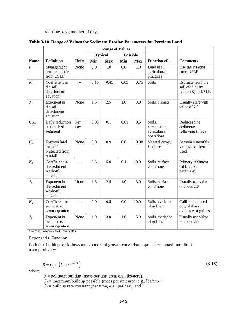
∆t = time, e.g., number of days.

Table 3-10. Ra nge of Values for Sediment Erosion Parameters for Pervious Land

Name onDefiniti Units

Range of Values

Function of... Comments Typical Possible

Min xMa Min Max P ement Manag

practice factor from USLE

None 0.0 1.0 0.0 1.0 Land use, agricultural practices

Use the P factor from USLE

Kr nt in

nt

Coefficie the soil detachme equation

-- 0.15 0.45 0.05 0.75 Soils Estimate from the soil erodibility factor (K) in USLE

Jr Exponent the soil

in

detachment equation

None 1.5 2.5 1.0 3.0 Soils, climate Usually start with value of 2.0

Caffix Daily reduction in detached sediment

Per day

0.03 0.1 0.01 0.5 Soils, compaction, agricultural operations

Reduces fine sediments following tillage

Csv Fraction land surface protected from rainfall

None 0.0 0.9 0.0 0.98 Vegetal cover, land use

Seasonal/ monthly values are often used

Ks Coefficient in the sediment washoff equation

-- 0.5 5.0 0.1 10.0 aceSoils, surf conditions

Primary sediment calibration parameter

Js Exponent in the sediment washoff equation

None 1.5 2.5 1.0 3.0 Soils, surface conditions

Usually use value of about 2.0

Kg Coefficient in soil matrix scour equation

-- 0.0 0.5 0.0 10.0 Soils, evidence of gullies

evidence of gulli

Calibration, used only if there is

es Jg Exponent in

soil matrix scour equation

None 1.0 3.0 1.0 5.0 Soils, evidence of gullies

Usually use value of about 2.5

Source: Donigian and Love 2003

Exponential Function Pollutant buildup, B, follows an exponential growth curve that approaches a maximum limit asymptotically:

B = C1 × (1− e 2 ∆t ) −C × (3-18) where B = pollutant buildup (mass per unit area, e.g., lbs/acre),

C1 = maximum buildup possible (mass per unit area, e.g., lbs/acre), C2 = buildup rate constant (per time, e.g., per day), and

3-45

C1tB = (3-19)

C2 + t

∆t = time, e.g., number of days.

Saturation Function Pollutant buildup, B, begins at a linear rate then slows down over time until a saturation value is reached:

where B = pollutant buildup (mass per unit area, e.g., lbs/acre), C1 = maximum buildup possible (mass per unit area, e.g., lbs/acre), C2 = half-saturation constant (days to reach half of the maximum buildup), and t = time, e.g., number of days.

Pollutant Washoff

The accumulated pollutants on a pervious land surface are washed off during runoff periods from a choice of available SWMM functions (Rossman 2005), which are all supported by SUSTAIN. These functions include the exponential washoff, rating curve washoff, and an event mean concentration (EMC).

Exponential Washoff The washoff load, W, is proportional to the product of runoff raised to the defined power C2 and to the amount of pollutant buildup remaining at each simulation timestep:

W = C1 × qs C2 × B (3-20)

where W = pollutant washoff load (mass per unit area per time, e.g., lbs/acre/hr), C1 = washoff coefficient, C2 = washoff exponent, qs = runoff rate per unit area (e.g., in./hr), and B = pollutant buildup (mass per unit area, e.g., lbs/acre).

Rating Curve Washoff The rate of pollutant washoff, W, is proportional to the runoff rate raised to the defined power C2:

W = C1 × qsC2 (3-21)

where W = pollutant washoff load (mass per unit area per time, e.g., lbs/acre/hr), C1 = washoff coefficient, C2 = washoff exponent, and qs = runoff rate (user-specified flow units, e.g., in./hr).

Event Mean Concentration (EMC) This is a special case of Rating Curve Washoff where the exponent is 1.0 and the coefficient C1 represents the washoff pollutant concentration in mass per volume. The typical EMCs for selected pollutants in urban runoff are shown in Table 3-11.

3-46

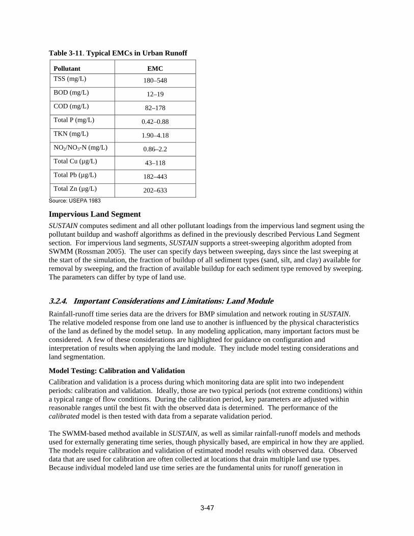
Table 3-11. Typical EMCs in Urban Runoff

Pollutant EMC TSS (mg/L) 180–548

BOD (mg/L) 12–19

COD (mg/L) 82–178

Total P (mg/L) 0.42–0.88

TKN (mg/L) 1.90–4.18

NO2/NO3-N (mg/L) 0.86–2.2

Total Cu (µg/L) 43–118

Total Pb (µg/L) 182–443

Total Zn (µg/L) 202–633 Source: USEPA 1983

Impervious Land Segment SUSTAIN computes sediment and all other pollutant loadings from the impervious land segment using the pollutant buildup and washoff algorithms as defined in the previously described Pervious Land Segment section. For impervious land segments, SUSTAIN supports a street-sweeping algorithm adopted from SWMM (Rossman 2005). The user can specify days between sweeping, days since the last sweeping at the start of the simulation, the fraction of bu ildup of all sediment types (sand, silt, and clay) available for removal by sweeping, and the fraction of available buildup for each sediment type removed by sweeping . The parameters can differ by type of land use.

3.2.4. Important Considerations and Limitations: Land Module Rainfall-runoff time series data are the drivers for BMP simulation and network routing in SUSTAIN. The relative modeled response from one land use to another is influenced by the physical characteristics of the land as defined by the model setup. In any modeling application, many important factors must be considered. A few of these considerations are highlighted for guidance on configuration and interpretation of results when applying the land module. They include model testing considerations and land segmentation.

Model Testing: Calibration and Validation Calibration and validation is a process during which monitoring data are split into two independent periods: calibration and validation. Ideally, those are two typical periods (not extreme conditions) within a typical range of flow conditions. During the calibration period, key parameters are adjusted within reasonable ranges until the best fit with the observed data is determined. The performance of the calibrated model is then tested with data from a separate validation period.

The SWMM-based method available in SUSTAIN, as well as similar rainfall-runoff models and methods used for externally generating time series, though physically based, are empirical in how they are applied. The models require calibration and validation of estimated model results with observed data. Observed data that are used for calibration are often collected at locations that drain multiple land use types. Because individual modeled land use time series are the fundamental units for runoff generation in

3-47

SUSTAIN, there is a need to ensure with reasonable confidence that modeled results are meaningful and applicable.

An ideal modeling data set for calibration includes m onitoring several smaller watersheds, each with relatively homogeneous land uses (i.e., low-density urban, high-density urban, forest) for a range of storm conditions. For each monitored storm event, the recomm ended data includes high-resolution precipitation, flow hydrograph, and discrete or composite water qualit y sampling for pollutants of concern. Using the observed precipitation, flow, an d water quality data, the model is developed and tested for each land use type on the basis of physical ch aracteristics of the drainage area. Standard calibration techniques are typically applied to assess how well the observed and the modeled time series data match.

A limitati on of any modeling effort is the inability to represent 100 percent of nature’s heterogeneity; the recognition of that fact influences the interpretation and application of calibrated model results. The setup of SUSTAIN is based on building representative land use times series data that allow users to make com parisons and extrapolate responses for current and potential fu ture land use and management conditions. Testing each land use and the combined behavior of mixed land use w atersheds against observed data is used to adjust model parameters for the best fit and to confirm model results. One com mon use of the calibrated data set is the extrapolation of re sults at one location to represent a response at other similar but ungaged locations. SUSTAIN includes land use reclassification to facilitate the application of models to various future or managed conditions and can be used to develop locally homogenized responses of similar land units. The primary ob jective of the model is to capture the unique essence of one type of land-use response relative to other types. When the available calibration data are limited, that objective becomes even more important for either extrapolating time series response from one calibrated area to another, or adopting loading estimates for various land uses from literature.

Particle Size Distribution Most land-based erosion and sediment simulation techniques compu te total eroded sediment load. Because the simulation land segments are discret ized by the land use category, erosion is simulated uniquely and is characteristic of that land use category. For sediment produced by each land use, particle size distribution is represented as fractional distribution of the total sediment . That means that the total land-based sediment load, multiplie d by the corresponding size fraction, gives the actual amount of sediment computed for each sediment si ze class. The user can allocate sediment into three classes ( sand, silt, and clay) . The three sediment classes are used to represent sed iment response behavior during transport in subsequent B MP or conduit m odules or both.

Particle size distribution a nd associated pollut ant concentrations pro vide an important linka ge to BMP simulation algorith ms. For example, BMPs that remove pollutant t hrough trapping and settling of sediments will be especia lly sensitive to the user-specified particle size distributions. If residence time within the BMP i s short, o nly larger particles might be re moved effe ctively. For ext ernally generated time series data, SUSTAIN supports the o ption to specify each sediment class as an independent time series rather than apply a size distribution to a bulk sediment m ass. This approach might be desirable in cases where p article size distribution changes dramatically during the course of a single storm event and detailed sediment mo nitoring data are available to justify the mode ling approach.

Land Segmentation Finally, depending on th e size of the watershed being modeled, regional considerations can influence the robustness and utility of t he modeled land units. In fact, the way land units are class ifie d from the onset can have a strong bearing on how representative or portable the modeled land unit response will be. For example, in some places, it might be sufficient to model land units on land use alone; whereas, in others, the use of a hydrologic response units (HRUs) approach might provide a better representation. An HRU

3-48

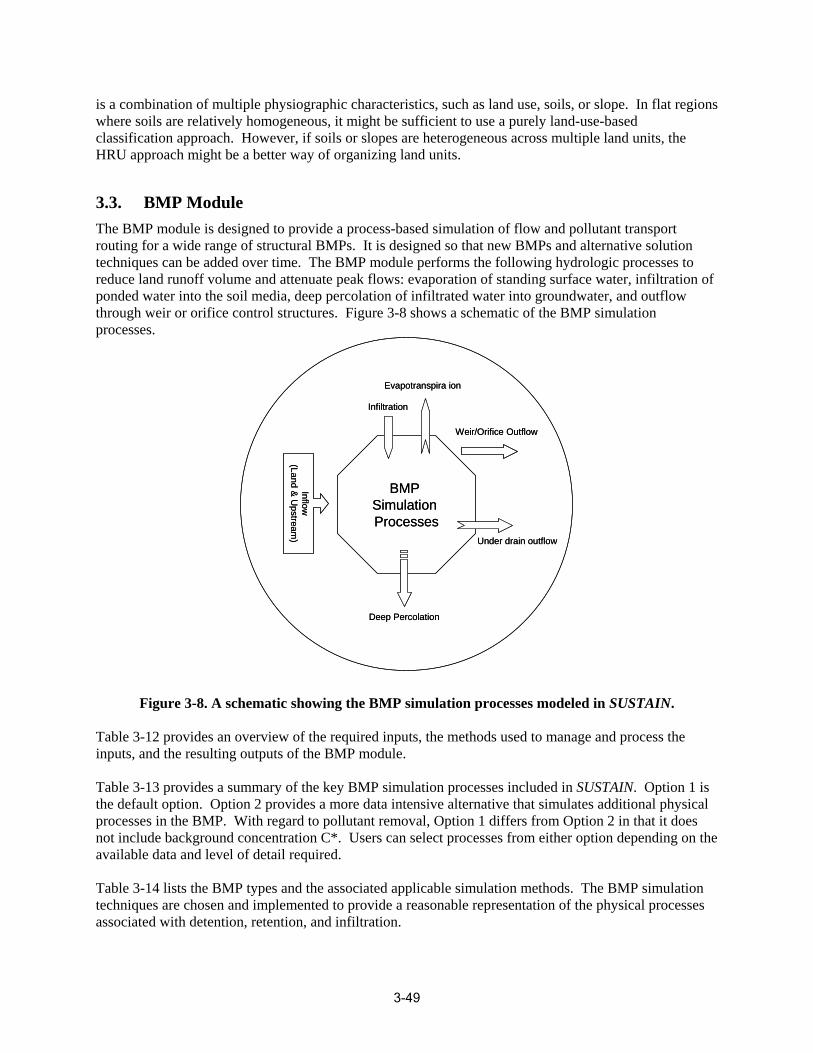
is a combination of multiple physiographic characteristics, such as land use, soils, or slope. In flat regions where soils are relatively homogeneous, it might be sufficient to use a purely land-use-based classification approach. However, if soils or slopes are heterogeneous across multiple land units, the HRU approach might be a better way of organizing land units.

3.3. BMP Module The BMP module is designed to provide a process-based simulation of flow and pollutant transport routing for a wide range of structural BMPs. It is designed so that new BMPs and alternative solution techniques can be added over time. The BMP module performs the following hydrologic processes to reduce land runoff volume and attenuate peak flows: evaporation of standing surface water, infiltration of ponded water into the soil media, deep percolation of infiltrated water into groundwater, and outflow through weir or orifice control structures. Figure 3-8 shows a schematic of the BMP simulation processes.

BMPSimulation Processes

Deep Percolation

Under drain outflow

Weir/Orifice Outflow

ra ionEvapotranspi

Infiltration

Inflo &

Uwpstr

(Landeam

)

BMP Simulation Processes

Deep Percolation

Under drain outflow

Weir/Orifice Outflow

ra ionEvapotranspi

Infiltration

Inflo &

U wpstr

(Land eam

)

Figure 3-8. A schematic showing the BMP simulation processes modeled in SUSTAIN.

Table 3-12 provides an overview of the required inputs, the methods used to manage and process the inputs, and the resulting outputs of the BMP module.

Table 3-13 provides a summary of the key BMP simulation processes included in SUSTAIN. Option 1 is the default option. Option 2 provides a more data intensive alternative that simulates additional physical processes in the BMP. With regard to pollutant removal, Option 1 differs from Option 2 in that it does not include background concentration C*. Users can select processes from either option depending on the available data and level of detail required.

Table 3-14 lists the BMP types and the associated applicable simulation methods. The BMP simulation techniques are chosen and implemented to provide a reasonable representation of the physical processes associated with detention, retention, and infiltration.

3-49

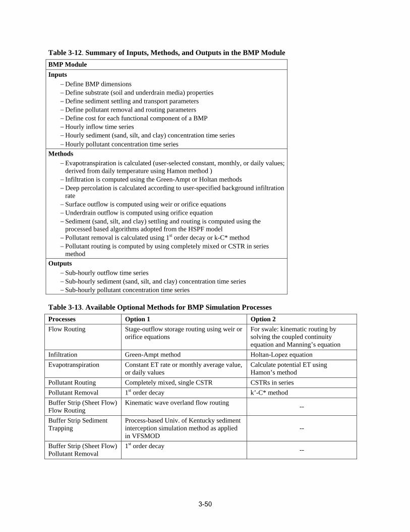
Table 3 12- . Summary of Inputs, Method s, and Outputs in the BMP Module BMP Module Inputs

− Define BMP dimensions − Define substrate (soil an − Define sediment settling

d underdrain media) properties and transport parameters

− Define cost for each functional component of a BMP − Hourly inflow time series − Hourly sediment (sand, silt, and clay) concentration time series

ourly pollutant concentration time series

− Define pollutant removal and routing parameters

− H Methods

− Eva (user-selected constant, monthly, or daily values; de ethod )

− In t or Holtan methods − Deep p user-specified background infiltration

rain outflow is computed using orifice equation − Sediment (sand, silt, and clay) settling and routing is computed using the

processed based rithms adopted from the HSPF model − Pollutant remova st

− Pollutant routing method

potranspiration is calculated rived from daily temperature using Hamon m filtration is computed using the Green-Amp

ercolation is calculated according to rate

− Surface outflow is computed using weir or orifice equations − Underd

al l

go is calculated using 1 order decay or k-C* method

is computed by using completely mixed or CSTR in series

Outputs − Sub-hourly outflow time series − Sub-hourly sediment (sand, silt, and clay) concentration time series − Sub-hourly pollutant concentration time series

Table 3-13. Available Optional Methods for BMP Simulation Processes Processes Option 1 Option 2 Flow Routing Stage-outflow storage routing using weir or

orifice equations For swale: kinematic routing by solving the coupled continuity equation and Manning’s equation

Infiltration Green-Ampt method Holtan-Lopez equation Evapotranspiration Constant ET rate or monthly average value,

or daily values Calculate potential ET using Hamon’s method

Pollutant Routing Completely mixed, single CSTR CSTRs in series Pollutant Removal 1st order decay k’-C* method Buffer Strip (Sheet Flow) Flow Routing

Kinematic wave overlan d flow routing --

Buffer Strip Sedimen ping

t Trap

Proce sed Uni Kentuc diment interc simul ethod plied in VFSMOD

ss-ba v. of ky se eption ation m as ap --

Buffer Strip (Sheet F tant Removal

low) Pollu

1st or cayder de --

3-50

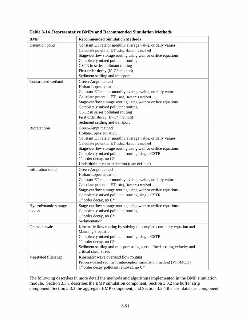
Table 3-14. Representative BMPs and Recommended Simulation Methods BMP Recommended Simulation Methods Detention pond Constant ET rate or monthly average value, or daily values

Calculate potential ET using Hamon’s method Stage-outflow storage routing using weir or orifice equations

uting

ort

Completely mixed pollutant ro CSTR in series pollutant routing First order decay (k’-C* method) Sediment settling and transp

Constructed wetland Green-Ampt method Holtan-Lopez equation Constant ET rate or monthly average value, or daily values Calculate potential ET using Hamon’s method Stage-outflow storage routing using weir or orifice equations Completely mixed pollutant routing CSTR in series pollutant routing First order decay (k’-C* method) Sediment settling and transport

Bioretention Green-Ampt method Holtan-Lopez equation Constan rate or monthly average value, or daily values Calculate potential ET using Hamon’s method Stage-outflow storage routing using weir or orifice equations Completely mixed pollutant routing, single CSTR

st

er defined)

t ET

1 order decay, no C* Underdrain percent reduction (us

Infiltration trench Green-Ampt method Holtan-Lopez equation Constant ET rate or monthly average value, or daily values Calculate potential ET using Hamon’s method

low storage routing using weir or orifice equations Completely mixed pollutant routing, single CSTR 1st order decay, no C*

Stage-outf

Hydrodyn amic sto erag Stage-outflow storage routing using weir or orifice equations device llutant routing

* Completely mixed po 1st order decay, no C Sedimentation

Grassed swale Kinematic flow routing by solving the coupled continuity equation and

, single CSTR 1st order decay, no C*

Manning’s equation Completely mixed pollutant routing

Sediment settling and transport using user defined settling velocity and critical shear stress

Vegetated filterstrip Kinematic wave overland flow routing Process-based sediment interception simulation method (VFSMOD)

st er decay pollutant removal, no C* 1 ord

The following describes in more detail the methods and algorithms implemented in the BMP simulation module. Section 3.3.1 describes the BMP simulation component, Section 3.3.2 the buffer strip component, Section 3.3.3 the aggregate BMP component, and Section 3.3.4 the cost database component.

3-51

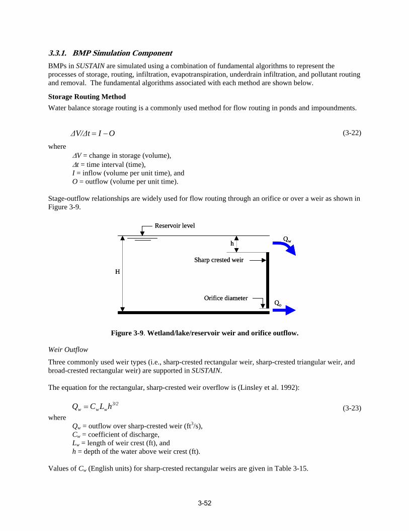
Q = C L h3/2

(3-23)w w w

3.3.1. BMP Simulation Component BMPs in SUSTAIN are simulated using a combination of fundamental algorithms to represent the processes of storage, routing, infiltration, evapotranspiration, underdrain infiltration, and pollutant routing and removal. The fundamental algorithms associated with each method are shown below.

Storage Routing Method Water balance storage routing is a commonly used method for flow routing in ponds and impoundments.

∆V/∆t = I − O (3-22)

where ∆V = change in storage (volume), ∆t = time interval (time), I = inflow (volume per unit time), and O = outflow (volume per unit time).

Stage-outflow relationships are widely used for flow routing through an orifice or over a weir as shown in Figure 3-9.

Reservoir level

h

Sharp crested weir

Orifice diameter

H

Reservoir level

Qw

Qo

h

Sharp crested weir

Orifice diameter

Qw

H

Qo

Figure 3-9. Wetland/lake/reservoir weir and orifice outflow.

Weir Outflow

Three commonly used weir types (i.e., sharp-crested rectangular weir, sharp-crested triangular weir, and broad-crested rectangular weir) are supported in SUSTAIN.

The equation for the rectangular, sharp-crested weir overflow is (Linsley et al. 1992):

where Qw = outflow over sharp-crested weir (ft3/s), Cw = coefficient of discharge, Lw = length of weir crest (ft), and h = depth of the water above weir crest (ft).

Values of Cw (English units) for sharp-crested rectangular weirs are given in Table 3-15.

3-52

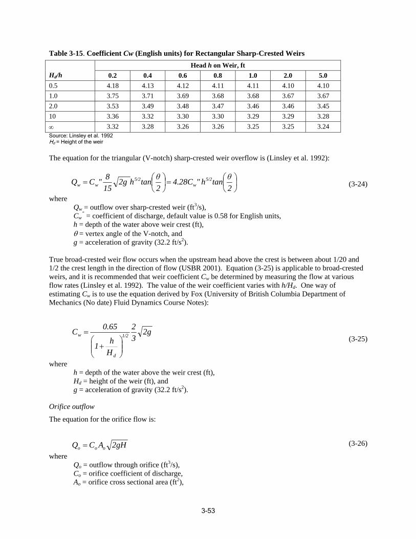
Table 3-15. Coefficient Cw (English units) for Rectangular Sharp-Crested Weirs

Hd/h Head h on Weir, ft

0.2 0.4 0.6 0.8 1.0 2.0 5.0 0.5 4.18 4.13 4.12 4.11 4.11 4.10 4.10 1.0 3.75 3.71 3.69 3.68 3.68 3.67 3.67 2.0 3.53 3.49 3.48 3.47 3.46 3.46 3.45 10 3.36 3.32 3.30 3.30 3.29 3.29 3.28 ∞ 3.32 3.28 3.26 3.26 3.25 3.25 3.24 Source: Linsley et al. 1992 Hd = Height of the weir

The equation for the triangular (V-notch) sharp-crested weir overflow is (Linsley et al. 1992):

Qw =C " w 8

15

θ θ⎜⎛tan⎛

⎜⎞⎟

⎞⎟⎠

5/2 5/22g h 4.28C " htan = (3-24)w2 2⎝ ⎠ ⎝ where

Qw = outflow over sharp-crested weir (ft3/s), Cw

” = coefficient of discharge, default value is 0.58 for English units, h = depth of the water above weir crest (ft), θ = vertex angle of the V-notch, and g = acceleration of gravity (32.2 ft/s2).

True broad-crested weir flow occurs when the upstr eam head above the crest is between about 1/20 and 1/2 the crest length in the direction of flow (USBR 2001). Equation (3-25) is applicable to broad-crested weirs, and it is recommended that weir coefficient Cw be determined by measuring the flow at various flow rates (Linsley et al. 1992). The value of the weir coefficient varies with h/Hd. One way of estimating Cw is to use the equation derived by Fox (University of British Columbia Department of Mechanics (No date) Fluid Dynamics Course Notes):

0.65 2C 2g

⎛ = 1/2w 3 (3-25)⎞h1+⎜⎜

⎝ ⎟⎟⎠H d

where h = depth of the water above the weir crest (ft), Hd = height of the weir (ft), and g = acceleration of gravity (32.2 ft/s2).

Orifice outflow

The equation for the or ifice flow is:

Qo =Co Ao 2gH (3-26)

where Qo = outflow through orifice (ft3/s), Co = orifice coefficient of discharge, Ao = orifice cross sectional area (ft2),

3-53

g = acceleration due to gravity (ft/s2), and H = depth of the water level above the orifice (ft).

Infiltration/Filtration SUSTAIN supports two options for the simulation of infiltration in BMPs: (1) the Holtan-Lopez equation adopted from the Prince George’s County BMP module (Tetra Tech 2001) and (2) the Green-Ampt equation (for details, see Section 3.2.2) as is applied in the SWMM (Rossman 2005).

Holtan-Lopez Empirical Model

The Holtan-Lopez empirical model computes the infiltration rate as a function of the actual available soil water storage, Sa, of the surface soil layer, as shown below (Maidment 1993):

f = GRI × A× S 1.4 + fc (3-27)a

where f = infiltration rate (in./hr), GRI = growth index of vegetation in percent maturity, varying from 0.1 to 1.0, A = infiltration capacity (an index representing surface-connected porosit y and density of plant roots), Sa = available storage in the surface layer (in.), and fc = constant final infiltration rate (in./hr).

In Equation (3-27), A is the vegetative parameter that characterizes surface-connected porosity and the density of plant roots, which affect infiltration (a value of 0.8 is a typical number for sod or vegetation that would be found in a BMP). fc is the final constant infiltration rate (in./hr), which is a function of the hydrologic soil group. The value of fc ranges from 0.3 in./hr for group-A soils to between 0.0 and 0.05 in./hr for group-D soils (Maidment 1993). In a continuous calculation, the available soil storage (Sa) and infiltration rate (f) are computed at each simulation time step. Available soil storage is updated each tim e increment and the infiltration is calculated.

This method was developed using th e premise that soil moisture storage, surface-connected porosity, and the effect of root density of the control soil layer are the dominant factors influencing the infiltration process.

A difficulty with using this method is estimating the control soil layer depth. For simulating the infiltration process, it is assumed that the soil column depth is the control depth because BMP devices normally have a confined soil/substrate layer.

Green-Ampt Infiltration Equation

This method is discussed in Section 3.2.2 in the hydrology component of land simulation module. The Green-Ampt equation can be applied to both surface runoff and BMP simulation.

When performing BMP infiltration simulation, the impact of the underdrain layer, the impermeable bottom layer, or both, on the infiltration process needs to be considered in the simulation. Because the Green-Ampt method can be applied to a layered soil column, the underdrain layer can be represen ted as a separate layer under t he soil column. In cases where an impermeable layer is present at the bottom of the soil column, the infiltration rate ceases when the soil storage capacity is reached.

A drawback of the Green-Ampt method is that it does not include a parameter to explicitly reflect the effect of the vegetation root zone on the infiltration rate.

3-54

Evapotranspiration Potential evapotranspiration (PET) time series can be estimated on the basis of the U.S. Weather Bureau Class A pan records with adjustment. For instance, the HSPF WDM utility estimates PET using the pan records, then the HSPF simulation model is used to adjust the time series for snow accumulation an d melt (Bicknell et al. 1997). When snow conditions are absent, only PET and precipitation are required. However, when snow conditions are considered, air temperature, rainfall, snow cover, water yield, and ice content of the snowpack are also re quired, and the evaporation data are adjusted. The input evaporation values are reduced to account for the fraction of the lan d segment covered by the snowpack.

Several methods are avail a ble to estimate PET. The Penman-Mont eith method (Maidment 1993) requires values for solar radiation, air temperature, relative humidity, and wind speed. The Priestley-Taylor method (Maidment 1993) require s solar radiation, air temperature, and relative humidity. The third, Hargreaves method (Maidment 1993) requires air temperature only.

SUSTAIN provides three options to estimate PET: (1) rely on the user-supplied monthly PET rate (2) calculate PET from the user-supplied pan evaporation time series input and mon thly pan coefficients, and (3) calculate the PET rate using Hamon’s method (1961).

Hamon’s (1961) method generates daily PET using air temperature, a monthly variable coefficient, the number of hours of sunshine (computed from latitude), and absolute humidity (computed from air temperature).

PET = C × D 2 × ρ (3-28)TS hr ws

where PET = daily PET (in.),

TS = monthly variable coefficient, and

Dhr = possible hours of sunshine computed as a function of latitude and time of year.

C

216.7 × pρ = ws (3-29)ws Tav + 273.3

where ρws = saturated water vapor density (absolute humidity) at daily mean air temperature (g/cm3) and Tav = mean daily air temperature ( °C).

⎡17.26939 × Tav ⎤

pws = 6.108 × exp ⎢ ⎥ (3-30)Tav + 273.3⎣ ⎦

where pws = saturated vapor pressure at the air temperature.

Hamon (1961) suggests a constant value of 0.0055 for CTS. However, monthly values can be specified to avoid underestimating PET in some areas, especially for the winter months.

3-55

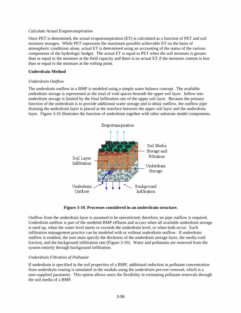
Calculate Actual Evapotranspiration

Once PET is determined, the actual evapotranspiration (ET) is calculated as a function of PET and soil moistu re storages. While PET represents the maximum possible achievable ET on the basis of atmospheric c onditions alone, actual ET is determined using an accounting of the status of the various components of the hydrologic budget. The actual ET is equal to PET when the soil moisture is greater than or equal to the moisture at the field capacity and there is no actual ET if the moisture content is less than or equal to the moisture at the wilting point.

Underdrain Method

Underdrain Outflow

The underdrain outflow in a BMP is modeled using a simple water balance concept. The available underdrain storage is represented as the total of void spaces beneath the upper soil layer. Inflow into underdrain storage is limited by the final infiltration rate of the upper soil layer. Because the primary function of the underdrain is to provide additional water storage and to delay outflow, the outflow pipe draining the underdrain layer is placed at the interface between the upper soil layer and the underdrain layer. Figure 3-10 illustrates the function of underdrain together with other substrate model components.

Figure 3-10. Processes considered in an underdrain structure.

Outflow from the underdrain layer is assumed to be unrestricted; therefore, no pipe outflow is required. Underdrain outflow is part of the modeled BMP effluent and occurs when all available underdrain stora ge is used up, when the water level meets or exceeds the underdrain level, or when both occur. Each infiltration management practice can be modeled with or without underdrain outflow. If underdrain outflow is enabled, the user must specify the thickness of the under drain storage layer, the media void fraction, and the background infiltration rate (Figure 3-10). Water and pollutants are removed from the system entirely through background infiltration.

Underdrain Filtration of Pollutant

If underdrain is specified in the soil properties of a BMP, additional reduction in pollutant concentration from underdrain routing is simulated in the module using the underdrain percent removal, which is a user-supplied parameter. This option allows users the flexibility in estimating pollutant removals through the soil media of a BMP.

3-56

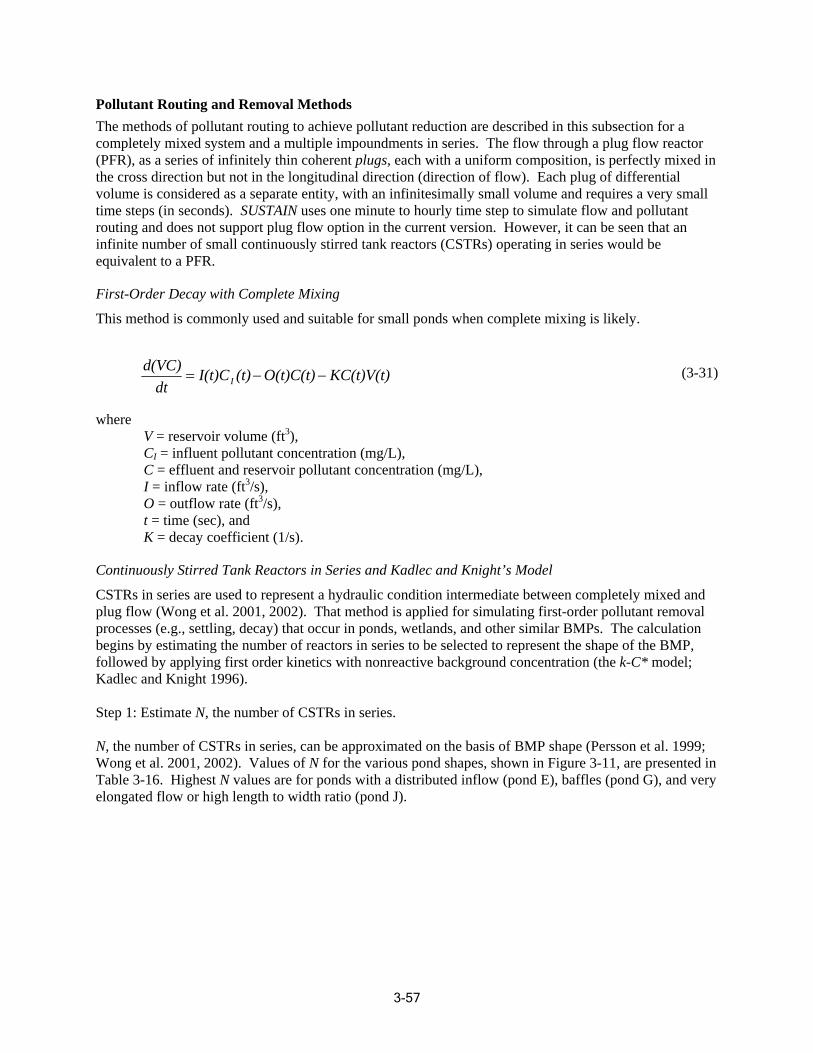
Pollutant Routing and Removal Methods The methods of pollutant routing to achieve pollutant reduction are described in this subsection for a completely mixed system and a multiple im poundments in series. The flow through a plug flow reactor (PFR), as a series of infinitely thin coherent plugs, each with a uniform composition , is perfectly mix ed in the cross direction but not in t he longi tudin al directio n (direction of flo w). Each plug of differential volume is considered as a sepa rate ent ity, with an infinitesimally small volume and requires a very sm all time steps (in seconds). SUSTAIN uses one minute to hour ly ti me step to simulate fl ow and pollutant routing and does not support plug flow option in the cur rent version. However, it can be seen that an infinite nu mber of small continuously stirred tank reactors (CSTRs) operating in series would be equivalent to a PFR.

First-Order Decay with Complete Mixing

This method is commonly used and suitable for small pon ds when complete mixing is likely.

d(VC) = I(t)CI (t) − O(t)C(t) − KC(t)V(t) (3-31)

dt

where V = reservoir volume (ft3), CI = influent pollutant concentration (mg/L), C = effluent and reservoir pollutant concentration (mg/L),

3I = inflow rate (ft /s), O = outflow rate (ft3/s), t = time (sec), and K = decay co efficient (1/s).

Continuously Stirred Tank Reactors in Series and Kadlec and Knight’s Model

CSTRs in series are used to represent a hydraulic condition intermediate between completely mixed and plug flow (Wong et al. 2001, 2002). That method is applied for simulating first-order pollutant removal processes (e.g., settlin g, decay) that occur in ponds, wetlands, and other similar BMPs. The calculation begins by estimating the number of reactors in series to be selected to represent the shape of the BMP, followed by applying first order kinetics with nonreactive background concentration (the k-C* model; Kadlec and Knigh t 1996).

Step 1: Estimate N, the number of CST Rs in series.

N, the number of CSTRs in series, can be appro ximated on the basis of BMP shape (Persson et al. 1999; Wong et al. 2001, 2002). Values of N fo r the various pond shapes, shown in Figure 3-11, are presented in Table 3-16. Highest N values are for ponds with a distributed inflow (pond E), baffles (pond G), and very elongated flow or high length to w idth ratio (pond J).

3-57

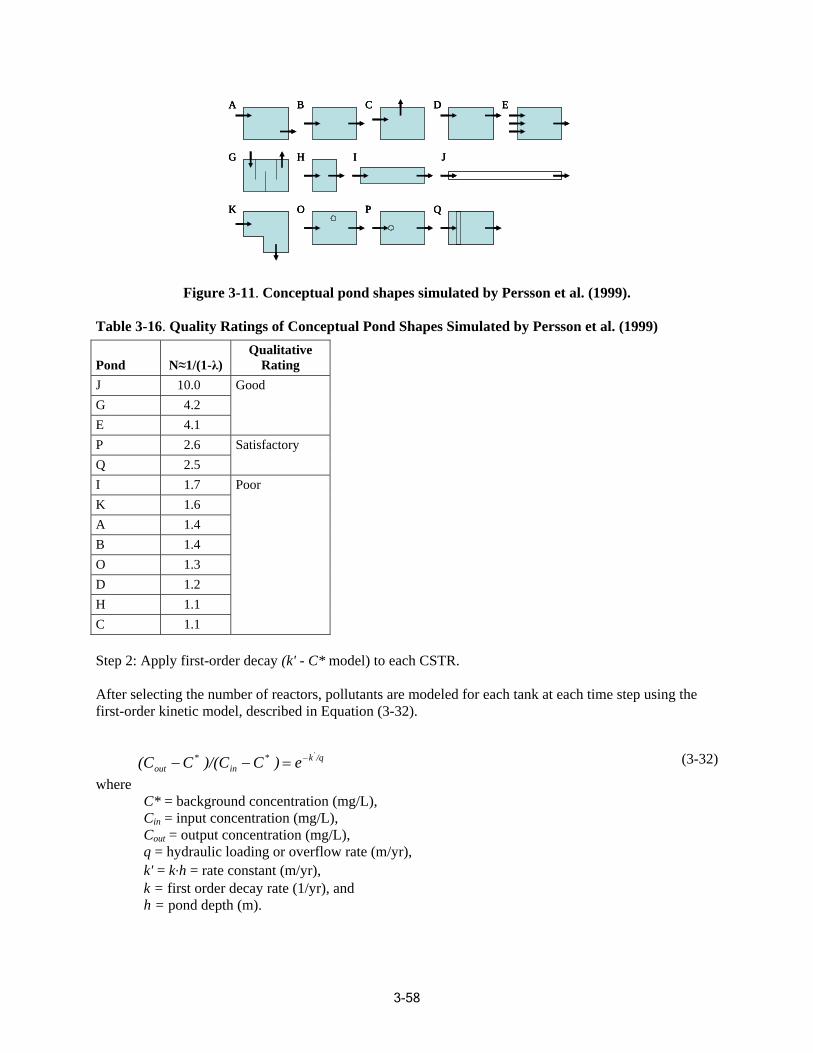
A B C D EA B C D EA B C D E

GGG HHH III JJJ

K O P QK O P QK O P Q

Figure 3-11. Conceptual pond shapes simulated by Persson et al. (1999).

Table 3-16. Quality Ratings of Conceptual Pond Shapes Simulated by Persson et al. (1999)

Pond N≈1/(1-λ) Rating Qualitative

J 10.0 Good G 4.2 E 4.1 P 2.6 Satisfactory Q 2.5 I 1.7 Poor K 1.6 A 1.4 B 1.4 O 1.3 D 1.2 H 1.1 C 1.1

Step 2: Apply first-order decay (k' - C* model) to each CSTR.

After selecting the number of reactors, pollutants are modeled for each tank at each time step using the first-order kinetic model, described in Equation (3-32).

* * −k' /q (3-32)(C − C )/(C − C ) = eout in

where C* = background concentration (mg/L), Cin = input concentration (mg/L), Cout = output concentration (mg/L), q = hydraulic loading or overflow rate (m/yr), k' = k∙h = rate constant (m/yr), k = first order decay rate (1/yr), and h = pond depth (m).

3-58

This equation is computed separately for each time step at each CSTR. The main difference between thi s equation and ordinary first-order decay modeling for a CSTR is the inclusion of C*, the background concentration, below which the effluent cannot fall. Another advantage of this method is that using an areal rate constant (units of depth/time) instead of a volumetric one (units of inverse time) helps avo id having to specify an average depth or the volume for odd natural configurations; instead, only the pond surface area is required to compute the hy draulic loading rate q.

Wong et al. (2002) recommend some k' and C* values as shown in Table 3-17, on the basis of limited model calibration for total suspended solids (TSS), total phosphorus (TP), and total nitrogen (TN) in urban areas near Melbourne. Those values should be used with caution. However, they could be used as a starting point in the absence of local d a ta.

Table 3-17. Recommended k' and C* Values

T nt Measuresreatme

k' (m/yr)

C* (mg/L)

TSS TP TN TSS TP TN S ation Basins ediment 15,000 12,000 1,000 30 0.18 1.7 Ponds 1,000 500 50 12 0.13 1.3 Vegetated Swales 15,000 12,000 1,000 30 0.18 1.7 Wetlands 5,000 2,800 500 6 0.09 1.3

Localized calibration can be performed to customize the simulation technique for specific areas. The C* and k' values can be determined or calibrated using monitoring data (particle size distribution in particular) and treatment measure design specifications.

3.3.2. Overland Flow Routing and Pollutant Interception The following algorithms for overland flow routing and pollutant interception simulation are employed in SUSTAIN for buffer strip simulation.

Kinematic Wave Overland Flow Routing Method for Filter Strip Simulation Overland flow through filter strips can be simulated using a kinematic wave method and solving the coupled continuity and Manning’s equations.

Mathematical Model

Continuity equation

∂h ∂q

+ = ie (t) (3-33)∂t ∂x

Manning’s equation

So 5/3 (3-34)q = q(h) = h n

where

h = overland flow depth (ft),

3-59

q = overland flow per unit width of the subcatchment (ft2/s), n = Manning’s roughness coefficient, ie = rainfall excess depth (ft/s), t = time (s), and So = subcatchment slope.

Initial conditi o n

h = 0; 0 ≤ x ≤ L; t = 0

Boundary condition

h = h0 ; x = 0; t > 0

where, h0 can be 0, a constant, or a time-dependent function, such as the incoming hydrograph from the adjacent subcatchment. The rainfall excess, ie, can be calculated from the hyetograph and Green-Ampt infiltration method at each time step.

Numerical Solution

The cou pled continuity equation and Manning’s equation are solved using Petrov-Galerkin (PG) formulation to compute the flow rate (q), velocity (v), and depth (h) throughout the plane for each time step. Kinematic shocks (oscillations in the solution) are introduced when a su dden change in conditions (e.g., slope, roughness, and inflow) occurs. For filter strip simulation, as the soil surface conditions are updated for each time step, the potential fo r kinematic shocks is further increased. The PG finite element method was found to reduce the amplitude and frequency of oscillations compared to a conventional Bubnov-Galerkin finite element solution, thus improving the model stability for situations that are subject to kinematic shocks (Muñoz-Carpena et al. 1993).

VFSMOD Algorithms for Sediment Interception The sediment interception algorithm used in VFSMOD considers that when runoff reaches the upstr eam edge of the filter, the vegetation provides a sudden increase in hydraulic resistance, which slows the flow, lowers its transport capacity, and causes depos ition of the coarse material (particle diameter dp > 0.0037 cm), which is carried mostly as bed-load transp ort. The sediment trapped in the first section of the filter forms a geometrical shape (the wedge zone), which is either triangular when Y (t) < H or trapezoidal after Y (t) = H, where Y (t) is the thickness of the deposited sediment layer and H is the effective height of th e vegetation.

The wedge zone is characterized by three well-defined zones: O, A, and B (Figure 3-12). The sediment loads at points 1 and 2 (gs1 and gs2) are calculated using the flow values provided by the overland flow routing module at points 1 and 2, and Einstein’s sediment bed-load transport function. After solving the sediment transport equations for a time step, new values of roughness and/or slope are selected as nodal values for the finite element grid in zones A(t) and B(t); while values for the grids in zones C(t) and D(t) remain unchanged. Changes in surface saturated hydraulic conductivity values are assumed to be negligible. The new surface parameters are fed back into the hydrology model for the next time step. The changes in the surface condition (i.e., slope and roughness) due to sediment deposition are recorded and passed back to the flow module.

3-60

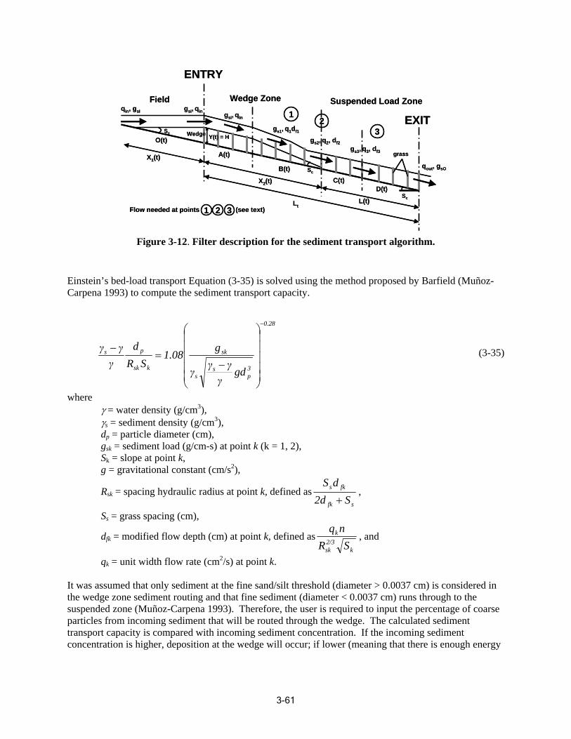
ENTENTRRYY

Flow needed at points 1 2 3 (see text)Lt

L(t)

X2(t) C(t)D(t)

X1(t)

O(t)

A(t)

B(t)

Suspended Load Zone

EXIT

Wedge Zone

12

3Sc

S qout, gsO

Fieldqin, gsI

c

grass

gsi, qin gsi, qin

gs1, q1df1

gs2, q2, df2gs3, q3, df3

Y(t) = H

Sc

Wedge

X1(t)

O(t)

A(t)

B(t)

Suspended Load Zone

EXIT

Wedge Zone

Flow needed at points 1 2 3 (see text) Lt

L(t)

X2(t) C(t) D(t)

1 2

3Sc

S qout, gsO

Field qin, gsI

c

grass

gsi, qin gsi, qin

gs1, q1df1

gs2, q2, df2 gs3, q3, df3

Y(t) = HWedge

Sc

Figure 3-12. Filter description for the sediment transport algorithm.

Einstein’s bed-load transport Equation (3-35) is solved using the method proposed by Barfield (Muñoz-Carpena 1993) to compute the sediment transport capacity.

−0.28⎞⎟ ⎟ ⎟ ⎟⎟

⎛⎜ ⎜ ⎜ ⎜⎜

−γ dγ g (3-35)skp =1.08s

γ Rsk S γ γ−k 3γ gds s pγ⎝ ⎠

where γ = water density (g/cm3), γ 3

s = sediment density (g/cm ), dp = particle diameter (cm), gsk = sediment load (g/cm-s) at point k (k = 1, 2), Sk = slope at point k, g = gravitational constant (cm/s2),

Rsk = spacing hydraulic radius at point k, defined as

Ss = grass spacing (cm),

Ssd fk ,2d S+fk s

, and 2/3

qk n Rsk Sk

dfk = modified flow depth (cm) at point k, defined as

q 2k = unit width flow rate (cm /s) at point k.

It was assumed that only sediment at the fine sand/silt threshold (diameter > 0.0037 cm) is considered in the wedge zone sediment routing and that fine sediment (diameter < 0.0037 cm) runs through to the suspended zone (Muñoz-Carpena 1993). Therefore, the user is required to input the percentage of coarse particles from incoming sediment that will be routed through the wedge. The calculated sediment transport capacity is compared with incoming sediment concentration. If the incoming sediment concentration is higher, deposition at the wedge will occur; if lower (meaning that there is enough energy

3-61

to transport sediment through the wedge and no deposition occurs), all sediment is transported to the suspended sediment zone (zones C(t) and D(t)).

After the downside of the wedge, two zones, C and D, form the suspended load zone. It was assumed th at on zone C, sediment has covered the indentations of the surface so that bed-load transport and deposition occur, but the soil slope is not significantly changed. All bed-load transported sediment is captured before reaching zone D so only suspended sediment is transported and deposited in this zone until the flow reaches the end of the filter. Flow values at point 3 and the exit point are needed for the calculation and are provided by the flow module. The trapping capacity (Tr) Equation (3-36) developed by Tollner e t al. (1976) is used to simulate the sediment trapping for the suspended load zone:

−0.91 −3 ⎛ V3Rs3 ⎞ ⎛ V f L ⎞⎡ 0.82 ⎤

⎢−1.05×10 ⎜ ⎟ ⎜⎜ ⎟⎟ ⎥ gs2 − gso ⎢⎣ ⎝ v ⎠ ⎝ V3h3 ⎠ ⎥

⎦ (3-36)Tr = = e gs2

where gs2 = sediment load at point 2 (g/cm-s), gso = sediment load at the output point (g/cm-s), V3 = mean velocity at point 3 (cm/s), Vf = fall velocity (cm/s), v = kinematic viscosity of water (cm2/s), and L = effective filter length (cm).

Particle Deposition and Sediment Transport

On the basis of the laboratory study by Deletic (2001) the particle deposition or trapping efficiency for sediment fraction s (particle with diameter of ds) can be estimated as a function of the particle fall number, Nf,s, which is calculated as:

lVsN f,s = (3-37)hV

where l is the flow length, Vs the Stokes’ settling velocity of particle size ds, and V is the average mean flow velocity between grass blades. The sediment trapping efficiency Tr,s is expressed as:

N 0.69

T = f,s (3-38)r,s 0.69N + 4.95f,s

The suspended sediment transport equation is expressed as:

2∂(hqs,s /q) ∂qs,s ∂ (hqs,s /q) (3-39)+ = Dis − λ qs s,s∂t ∂x ∂x2

where qs,s is the sediment loading rate of fraction s per unit width, Dis is the dispersion coefficient, and λs is the trapping efficiency for fraction s per unit length calculated as λs=Tr,s/l.

3-62

Terrain Surface Level and Slope Changes

The rise in the surface level, z, is modeled as the integral of trapped particles of all fractions of particle sizes and is expressed as:

∂z(x,t) 1 1

= λsqs,sds (3-40)∫∂ 1 − p ρst s

where p is the porosity of deposited sediment.

The water quality for the pollutant (other than suspended sediment) is simulated by applying the mos t commonly used first order decay model. A first order decay is equivalent to an exponential decay, represented by the Equation (3-41).

Ct =C0 e−kt (3-41)

where Ct = concentration at time t (mass per volume), C0 = initial concentration at time zero (mass per volume), and k = reaction rate (per timestep).

For the current phase of SUSTAIN development, the decision was mad e to include this complex, process-based simulation for filter strip simulations. This model is CPU intensive and, thus, is not used during the optimization process. Its purpose in SUSTA IN is for eval uation of filte r strip performance only (see Section 3.3.6). Future phases will include a s implified m ethod that ca n be incorporated into theoptimization module.

3.3.3. Aggregate BMP Component The aggregate BMP component provides an optiona l method for assessing the comb ined impa ct of multiple BMPs on the watershed runoff and pollut ant load. The form ulation was developed to represent the aggregate characteristics of distri buted BMP, while reducing the user effort for m odel setup and computation time needed for sim ulation and optim ization. While th e BMP module in SUSTAIN performs explicit simulation of individual BMP pract ices for a defined manage ment ar ea, the aggregate BMP component evalua tes storage and infiltration characteristics for multiple BMPs simultaneously without explicit recognition of their spatial distribution and routing characteristics in the selected watershed.

As illustrated in Figur e 3-13, an aggregate B MP consists of a series of process-based compone nts, including on-site inter ception, on-si te treatm ent, routing a ttenuation, a nd regional storage/treatment. For the aggregate BMPs, users are asked to input des ign drain age area and number of units for each aggregate BMP component. Each component can be used to repres ent one of a number of individual BM Ps. For example, on-site interception can be represented as a cistern, rain barrel, or green roof, while on-site treatment can be bioretention, porous pavement, or an infiltration trench. Each individual component can be enabled or disabled according to th e desired functionality and sized and parameterized using the BMP templates that are identical to that of the individual BMPs.

3-63

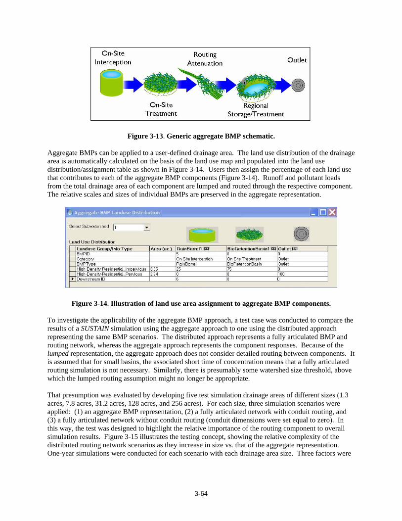
Figure 3-13. Generic aggregate BMP schematic.

Aggregate BMPs can be applied to a user-defined drainage area. The land use distribution of the drainage area is automatically calculated on the basis of the land use map and populated into the land use distribution/assignment table as shown in Figure 3-14. Users then assign the percentage of each land use that contributes to each of the aggregate BMP components (Figure 3-14). Runoff and pollutant loads from the total drainage area of each component are lumped and routed through the respective component. The relative scales and sizes of individual BMPs are preserved in the aggregate representation.

Figure 3-14. Illustration of land use area assignment to aggregate BMP components.

To investigate the applicability of the aggregate BMP approach, a test case was conducted to compare the results of a SUSTAIN simulation using the aggregate approach to one using the distributed approach representing the same BMP scenarios. The distributed approach represents a fully articulated BMP and routing network, whereas the aggregate approach represents the component responses. Because of the lumped representation, the aggregate approach does not consider detailed routing between components. It is assumed that for small basins, the associated short time of concentration means that a fully articulated routing simulation is not necessary. Similarly, there is presumably some watershed size threshold, above which the lumped routing assumption might no longer be appropriate.

That presumption was evaluated by developing five test simulation drainage areas of different sizes (1.3 acres, 7.8 acres, 31.2 acres, 128 acres, and 256 acres). For each size, three simulation scenarios were applied: (1) an aggregate BMP representation, (2) a fully articulated network with conduit routing, and (3) a fully articulated network without conduit routing (conduit dimensions were set equal to zero). In this way, the test was designed to highlight the relative importance of the routing component to overall simulation results. Figure 3-15 illustrates the testing concept, showing the relative complexity of the distributed routing network scenarios as they increase in size vs. that of the aggregate representation. One-year simulations were conducted for each scenario with each drainage area size. Three factors were

3-64

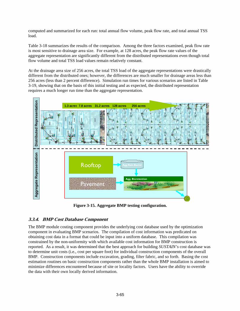
computed and summarized for each run: total annual flow volume, peak flow rate, and total annual TSS load.

Table 3-18 summarizes the results of the comparison. Among the three factors examined, peak flow rate is most sens itive to drainage area size. For example, at 128 acres, the peak flow rate values of the aggregate representation are significantly different from the distributed representations even though total flow volume and total TSS load values remain relatively constant.

At the drainage area size of 256 acres, the total TSS load of the a ggregate representations were drastically different from th e distributed ones; however, the differences are much smaller for drainage areas les s than 256 acres (less than 2 percent difference). Simulation run times f or va rious scenarios are listed in T able 3-19, showing that on the basi s of this initial testing and as expected, t he distributed representation requires a m uch lon ger run time than the aggregate representation.

Dis

tri

epre

bute

d R

sent

atio

nA

ggr

on

egat

e R

epre

sent

ati

Rooftop

Pavement

Agg Rain Barrel

Agg. Bioretention

1.3 acres 7.8 acres 31.2 acres 128 acres 256 acres

Figure 3-15. Aggregate BMP testing con figuration.

3.3.4. BMP Cost Database Component The BMP mod ule c o sting component provides the underlying cost dat abase used by the optimizatio ncomponent in evaluating BMP scenarios. The compilation of cost inform ation was predicated on obtaining cost data in a format that could be input into a uniform datab ase. This compilation was constrained by the non-uniformity with which available cost informati on for BMP cons truction is reported. As a result, it was determined that the best a pproach for building SUSTAIN’s cost database was to determine u nit co s ts (i.e., cost per square foot) for individual construction components of the overall BMP. Construction components include excavation, grading, filter fabric, and so forth. Basing the cost estimation routines on basic construction components rather than the whole BMP installation is aimed to minimize differences encountered because of site or locality factors. Users have the ability to override the data with their own locally derived information.

3-65

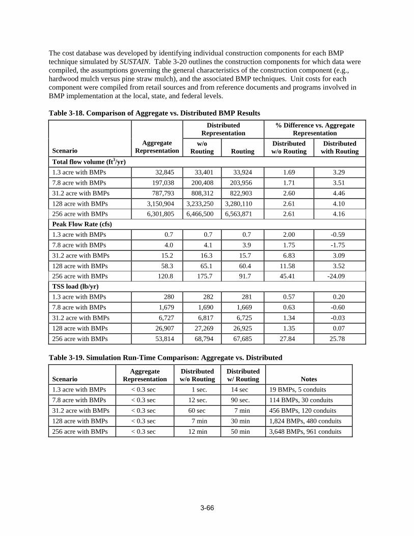
The cost database was developed by identifying individual construction components for each BMP technique simulated by SUSTAIN. Table 3-20 outlines the construction components for which data were compiled, the assumptions governing the general characteristics of the construction com ponent (e.g., hardwood mulch versus pine straw mulch ), and the associated BMP techniques. Unit costs for each component were compiled from retail sources and from reference documents and programs involved in BMP implementation at the local, state, and federal levels.

Table 3-18. Comparison of Aggregate vs. Distributed BMP Results

Scenario Aggregate

Representation

Distributed Representation

% Difference vs. Aggregate Representation

w/o Routing Routing

Distributed w/o Routing

Distributed with Routing

Total flow volume (ft3/yr) 1.3 acre with BMPs 32,845 33,401 33,924 1.69 3.29 7.8 acre with BMPs 197,038 200,408 203,956 1.71 3.51 31.2 acre with BMPs 787,793 808,312 822,903 2.60 4.46 128 acre with BMPs 3,150,904 3,233,250 3,280,110 2.61 4.10 256 acre with BMPs 6,301,805 6,466,500 6,563,871 2.61 4.16 Peak Flow Rate (cfs) 1.3 acre with BMPs 0.7 0.7 0.7 2.00 -0.59 7.8 acre with BMPs 4.0 4.1 3.9 1.75 -1.75 31.2 acre with BMPs 15.2 16.3 15.7 6.83 3.09 128 acre with BMPs 58.3 65.1 60.4 11.58 3.52 256 acre with BMPs 120.8 175.7 91.7 45.41 -24.09 TSS load (lb/yr) 1.3 acre with BMPs 280 282 281 0.57 0.20 7.8 acre with BMPs 1,679 1,690 1,669 0.63 -0.60 31.2 acre with BMPs 6,727 6,817 6,725 1.34 -0.03 128 acre with BMPs 26,907 27,269 26,925 1.35 0.07 256 acre with BMPs 53,814 68,794 67,685 27.84 25.78

Table 3-19. Simulation Run-Time Comparison: Aggregate vs. Distributed

Scenario Representation Aggregate

w/o Routing Distributed

w/ Routing Distributed

Notes 1.3 acre with BMPs < 0.3 sec 1 sec. 14 sec 19 BMPs, 5 conduits 7.8 acre with BMPs < 0.3 sec 12 sec. 90 sec. 114 BMPs, 30 conduits 31.2 acre with BMPs < 0.3 sec 60 sec 7 min 456 BMPs, 120 conduits 128 acre with BMPs < 0.3 sec 7 min 30 min 1,824 BMPs, 480 conduits 256 acre with BMPs < 0.3 sec 12 min 50 min 3,648 BMPs, 961 conduits

3-66

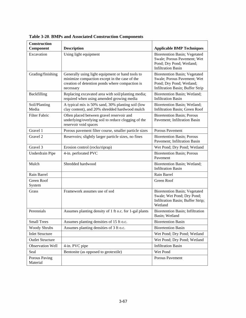
Table 3-20. BMPs and Associated Construction Components Construction Component Description Applicable BMP Techniques Excavation Using light equipment Bioretention Basin; Vegetated

Swale; Porous Pavement; Wet

ion Basin Pond; Dry Pond; Wetland; Infiltrat

Grading/finishing Generally using light equipment or hand to minimize compaction except in the case of the

ols to

creation of detention ponds where compaction is necessary

Swale; Porous P Bioretention Basin; Vegetated

avement; Wet Pond; Dry Pond; Wetland; Infiltration Basin; Buffer Strip

Backfilling Replacing excavated area with soil/planting media; required when using amended growing media

Bioretention Basin; Wetland; Infiltration Basin

Soil/Planting Media

A typical mix is 50% sand, 30% planting soil (low clay content), and 20% shredded hardwood mulch

Bioretention Basin; Wetland; Infiltration Basin; Green Roof

Filter Fabric Often placed between gravel reservoir and underlying/overlying soil to reduce clogging of the reservoir void spaces

Bioretention Basin; Porous Pavement; Infiltration Basin

Gravel 1 Porous pavement filter course, smaller particle sizes Porous Pavement Gravel 2 Reservoirs; slightly larger particle sizes, no fines Bioretention Basin; Porous

Pavement; Infiltration Basin Gravel 3 Erosion control (rocks/riprap) Wet Pond; Dry Pond; Wetland Underdrain Pipe 4-in. perforated PVC Bioretention Basin; Porous

Pavement Mulch Shredded hardwood Bioretention Basin; Wetland;

Infiltration Basin Rain Barrel Rain Barrel Green Roof System

Green Roof

Grass Framework assumes use of sod Bioretention Basin; Vegetated Swale; Wet Pond; Dry Pond; Infiltration Basin; Buffer Strip; Wetland

Perennials Assumes planting density of 1 ft o.c. for 1-gal plants Bioretention Basin; Infiltration Basin; Wetland

Small Trees Assumes planting densities of 15 ft o.c. Bioretention Basin Woody Shrubs Assumes planting densities of 3 ft o.c. Bioretention Basin Inlet Structure Wet Pond; Dry Pond; Wetland Outlet Structure Wet Pond; Dry Pond; Wetland Observation Well 4-in. PVC pipe Infiltration Basin Seal Bentonite (as opposed to geotextile) Wet Pond Porous Paving Material

Porous Pavement

3-67

Unit Cost Data Sources Costs for BMP constru ction com ponents were obtained from the following sources.

Wholesale/Retail Bulk Material Pricing

Several wholesale or retail companies were inventoried to p rovide bulk material pricing. Retailers were contacted to provide unit pricing for various raw materials such as mulch, sand, stone, and other commercial landscape mat erials. Retailers were also contacted to provide pricing for rain barrels. Unit cost data were compiled in 200 7.

EPA Stormwater Technology Fact Sheets

EPA’s Office of Water Municipal Technology Assessment Program sup ports innovative and alternative technology deve lopment through a number of efforts and partners. In 1999 the program produced a series of Stormwater Technology Fact Sheets (832-F-99-001 to 048), which are at http://www.epa.gov/owmitnet/mtb/ mtbfact.htm . The series provides information on advantages and disadvantages, design criteria, operations and maintenance, performance, and cost estimates re garding a range of managemen t technolog ies including biorete ntion, catch basins, flow diversion, infiltra tion trenches, modular sys tems, porous pavement, a nd others.

California Department of Transportation (CALTRANS)

In the late 1990s, CALTRANS began a stud y to evaluate structural BMPs for stormwater treatment. Among other things, the study ev aluated removal efficiencies, capital costs, and annual operation and maintenance (O&M) costs of individual applications.

Fairfax County BMP Fact Sheets

Fairfax County, Virgin ia, developed 25 fact sheets for inclusion in the county ’s Public Facilities Manual that present an overview of the manag ement strategies and technologies for various current or p otential BMP/LID techniques used in the county. The fact sheets address seven different BMP categories including: (1) bioretent ion systems, (2) filtering technologies, (3) permeable pavements, (4) s it e design strategies, (5) soil amen dments, (6) vegetative sy stems, and (7) water conservation/reuse. The information in each fact sheet is consistent so that relative comparisons can be m ade on the critical design, construction, and maintenance issues. Information includes a general description of the BMP, water quality and quant ity controls, l ocation; design construction and materials, cost, maintenance, performance and inspec tion, and potential LEED (Leaders hip in Energy and Environmental De sign) credits. The fact sheets are at http://www.lowimpactdevelopment.org/fairfax.htm#ffx factshee t.

Natural Resources Conservation Service (NRCS) Cost Share Data

The U.S. Department of Agriculture’s (USDA’s) NRCS program Web site provides cost lists and tools developed by NRCS field office staff to support BMP cost-sharing programs under the department’s Environmental Quality In centives Program and other programs. Documents containing unit cost data for BMP com ponents are available for various years for 34 states.

Michigan Department of Environmental Qua lity’s (DEQ’s) 319 BMP Cost Database

The Michigan DEQ’s N onpoint Source Program administers the CWA section 319 grant prog ram fo r the state. It requires grantees to submit BMP cost share information for purposes of tracking the cost and location of BM Ps installed with DEQ Nonpoint Source grant funding and documenting expe nses for cost-share practices. DEQ is required to produce annual reports for the EPA and the Michigan legislature to detail the use of state and federal grant funds. In addition, the data are also used to share information about specific practices with current and potential grant recipients. The SUSTAIN cost database adapted

3-68

cost data for certain practices such as green roofs and porous pavement because they were reported in the same units as the cost m odule database. Costs for other relevant BMPs are reported in the DEQ BMP Cost Share database; however, component costs are not broken down. As a result, these data were not used.

Green Roofs

EPA’s Heat Island Web site and the Great Lakes Water Institute’s Web site provide installation and maintenance costs per u nit for green roofs in urban a reas. The Web sites are http://www.epa.gov/hea tisland/mitigation/greenroofs.htm http://www.glwi.uwm.edu/research/genomics/ecoli/greenroof/roofinstall.php#costs.

Minnesota Stormwater Manual (version 1.1)

The Minnesota Stormwater Manual (Minnesota Pollution Control Agency 2005) provides unit costs for several BMPs. The Stormwater Manual discusses a variety of BMP approaches designed to lessen the impacts of urban development. The Manual explores an array of BMPs that can be implemen ted to control sediment and reduce runoff in a practical and flexible manner.

Cost Database The cost database in the BMP module is a Microsoft Access database containing records related to unit costs of BMP construction components releva nt to the techniques simulated by SUSTAIN. In addition to the unit cost per compo nent, each record contains informatio n related to the source of the data and, to the extent possible, the year or general tim e period from which the cost data were re corded. In addition, O&M cost estimates were available for a limited number of records. All unit cost data were entered into the unit cost table using the unit in the original source; conversions to a consisten t unit of measure take place in the system using appropriate conversion factors.

Using the Cost Component The Cost Component provides the flexibility of choosing the construction components and the associated costs for estimating the total cost of the BMP.

User Data

Users also have the option to enter their own cost data as well a s operations and maintenance costs.

Selection of Data

Cost estimates in the database are taken from sources across the country; however, not all states and regions are represented. Users can choose to base cost estimates on an average of all data in the database or they can choose to use only select sources of data if they deem specific sources to be adequately representative. In addition, the interface allows users the option of not including specific components when calculating the unit cost of a BMP. For example, in an area where it is not necessary to incl ude an impermeable seal on the bottom of a wet detention pond, the cost component can be turned off. O&M data were limited and, thus, are not included in the cost database.

Table 3-21 through Table 3-26 provide additional information related to fields and tables that compo se the database.

3-69

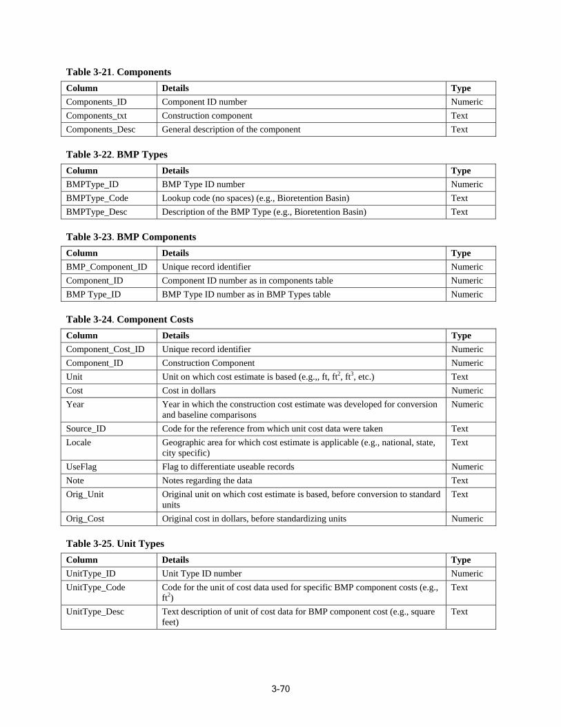
Table 3-21. Components Column Details Type Components_ID Component ID number Numeric Components_txt Construction component Text Components_Desc General description of the component Text

Table 3-22. BMP Types Column Details Type BMPType_ID BMP Type ID number Numeric BMPType_Code Lookup code (no spaces) (e.g., Bioretention Basin) Text BMPType_Desc Description of the BMP Type (e.g., Bioretention Basin) Text

Table 3-23. BMP Components Column Details Type BMP_Component_ID Unique record identifier Numeric Component_ID Component ID number as in components table Numeric BMP Type_ID BMP Type ID number as in BMP Types table Numeric

Table 3-24. Component Costs Column Details peTy Component_Cost_ID Unique record identifier Numeric Component_ID Construction Component Numeric Unit Unit on which cost estimate is based (e.g.,, ft, ft , ft , etc.) 2 3 Text Cos t Cost in dollars Numeric Year developed for conversion Year in which the construction cost estimate was

and baseline comparisons Numeric

Source_ID taken Code for the reference from which unit cost data were Text Locale state,Geographic area for which cost estimate is applicable (e.g., national,

city specific) Text

UseFlag Flag to differentiate useable records Numeric Note Notes regarding the data Text Orig_Unit Original unit on which cost estimate is based, before conversion to standard

units Text

O srig_Co t Original cost in dollars, before standardizing units Numeric

Table 3-25. Unit Types Column Details Type UnitType_ID Unit Type ID number Numeric UnitType_Code Code for the unit of cost data used for specific BMP component costs (e.g.,

ft2) Text

UnitType_Desc Text description of unit of cost data for BMP component cost (e.g., square feet)

Text

3-70

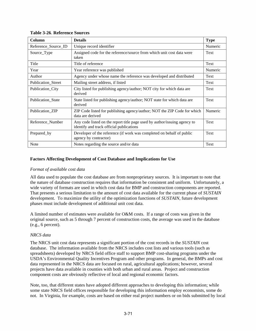
Table 3-26. Reference Sources Column Details Type Reference_Source_ID Unique record identifier Numeric Source_Type Assigned code for the reference/source from which unit cost data were

taken Text

Title Title of reference Text Year published Year reference was eric Num Author A ho fe ev gency under w se name the re rence was d eloped and distributed tTex Publication_Street Mailing street address, if listed Text Publication_City City lis r publishing ency/author OT city for whi ata are

derived ted fo ag ; N ch d Text

Publication_State State listed for publishin ency/author; NOT state for which data are derived

g ag Text

Publication_ZIP ZIP Co sted for publi ng agency/ r; NOT the ZIP Code for which data ar ved

de li e deri

shi autho eric Num

Reference_Number Any co sted on the re title page by author/issu ency to identif official publications

de li port used ing ag y and track

Text

Prepared_by Develop the referen f work wa pleted on beh ublic agency contractor)

er of ce (i s com alf of p by

Text

Note Notes regarding the source and/or data Text

Factors Affecting Developm ent of Cost Database and Implications for Use

Format of available cost data

All data used to populate the cost database are from nonproprietary sources. It is important to note that the nature of database construction requ ires that information be consistent and uniform. Unfortunately, a wide variety of formats are used in which cost data for BMP and construction components are reported. That presents a serious limitation to the amount of cost data available for the current phase of SUSTAIN development. To maximize the utility of the optimization functions of SUSTAIN, future development phases must include development of additional unit cost data.

A limited number of estimates were available for O&M costs. If a range of costs was given in the original source, such as 5 through 7 percent of construction costs, the average was used in the database (e.g., 6 percent).

NRCS data

The NRCS unit cost data represents a significant portion of the cost records in the SUSTAIN cost database. The information available from the NRCS includes cost lists and various tools (such as spreadsheets) developed by NRCS field office staff to support BMP cost-sharing programs under the USDA’s Environmental Quality Incentives Program and other programs. In general, the BMPs and cost data represented in the NRCS data are focused on rural, agricultural applications; however, several projects have data available in counties with both urban and rural areas. Project and construction component costs are obviously reflective of local and regional economic factors.

Note, too, that different states have adopted different approaches to developing this information; while some state NRCS field of fices responsible for developing this information employ economists, some do not. In Virginia, for example, costs are based on either real project numbers or on bids submitted by local

3-71

contractors for typical applications. Atypical (expensive, technically complicated, or unusual) projects are generally excluded from the universe of estimates used to generate average cost lists.

The cost share data for 28 states were accessed and reviewed during development of the database, and appropriate records were selected for inclusion on the basis of consistency with the BMPs and components represented in SUSTAIN, as well as the applicability of units for which costs were reported. The potential exists that cost estimates derived from the NRCS data are low, relative to costs for proje cts in more urban areas, which might be expected to have higher unit costs because of higher operating, equipment rental, land, and other costs. Efforts were made to select data for inclusion in the database to address this potential for underestimation. For example, the Alabama cost estimator spreadsheet includes four records related to unit costs for the SUSTAIN component backfill. The analogous component in the Alabama Cost Estimator spreadsheet is called Earthfill. Cost estimates are available for < 3,000 yd3; 3,000–10,000 yd3; 10,000–30,000 yd3; and 30,000+ yd3. Unit costs for the smallest volume (< 3,000 yd3) are highest; therefore, it was the estimate selected for inclusion in the SUSTAIN cost estimate database. Where the NRCS data provide multiple unit costs for a c omponent, the highest cost is used.

Because the NRCS data represent such a significant proportion of the publicly available unit cost data related to implementation and construction of BMPs, they were included in the cost database for SUSTAIN. However, in recognition of the potential limitations associated with applying those data to urban areas, users may opt to exclude all NRCS data from cost calculations. Note that excluding NRCS data will result in a more restricted data set from which the m odel’s cost estimates will be based.

3.3.5. Summary of Management Practices and Treatment Processes in SUSTAIN SUSTAIN provides multiple ways for simulating management practices that are widely used to treat runoff and mitigate flow volumes. Treatment processes may be grouped into the following categories:

• Storage/detention or flow attenuation (i.e., those detaining and/or attenuating water) • Infiltration (i.e., those infiltrating water to the ground) • Filtration (i.e., those passing water through a porous medium) • Evapotranspiration (i.e., those losing water from surface and/or soil column) • Water quality (i.e., those performing pollutant removal)

Table 3-27 lists the structural BMP types handled by SUSTAIN and the associated treatment processe s.

3.3.6. Important Considerations and Limitations of the BMP Module Selecting an Appropriate Simulation Method The BMP module provides an array of simulation options with varying degrees of sophistication in t he required input and computational rigor. Such options provide flexibility for users to customize their problem formulations to suit the project needs. The user should carefully select the method or approach considering the overall problem formulation, availability of supporting data, and expected outco mes. For example, users can choose between the two infiltration options provided: the simple Holtan infiltration method or the iterative Green-Ampt infiltration method. To optimize BMP selection for a large study area having several infiltration BMPs, it might be advantageous to select the Holtan method over the Green-Ampt method because it might result in shorter computation time (e.g., reduced runtime for a single run by several seconds). Because it might be required to perform hundreds or thousands of BMP simulations during an optimization analysis, the accumulated run time savings of a few seconds per run

3-72

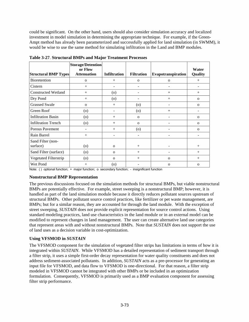
could be significant. On the other hand, users should also consider simulation accuracy and localized investm ent in model simulation in determining the appropriate technique. For example, if the Green-Ampt method has already been parameterized and successfully applied for land simulation (in SWMM), it would be wise to use the same method for sim ulating infiltration in the Land and BMP modules.

Table 3-27. Structural BMPs and Major Treatm ent Processes

Structural BMP Types Attenuation

Storage/Detention or Flow

Infiltration nFiltratio Evapotranspiration Water

Quality Bio retention o + o o + Cistern + - - - -Constructed Wetland + (o) - + + Dry Pond + (o) - + o Grassed Swale o + (o) - o Green Roof (o) - (o) + -Infiltration Basin (o) + o - o Infiltration Trench (o) + o - o Porous Pavement - + (o) - o Rain Barrel + - - - -San surf

d Filter (non­ace) (o) o + - +

Sand Filter (surface) (o) o + - + Vegetated Filterstrip (o) o + o + Wet Pond + (o) - o o

Note: ( ) optional function; + major function; o secondary function; – insign ificant function

Nonstructural BMP Representation The previous discussions focused on the simulation methods for structural BMPs, but viable nonstructural BMPs are potentially effective. For example, street sweeping is a nonstructural BMP; however, it is handled as part of the land sim ulation module because it directly reduces pollutant sources upstream of structural BMPs. Other pollutant sourc e control practices, like fertilizer or pet waste management, are BMPs; but for a s imilar reason, they are accounted for through the land module. With the exception of street sweeping, SUSTAIN does not provide explicit representation for source control actions. Using standard mode ling practices, land use characteristics in the land module or in an external model can be modified to represent chan ges in land management. The user can create alternative land use categories that represent areas with and wi thout nonstructural BMPs. Note that SUSTAIN does not support the use of land uses as a decision variable in cost-optimization.

Using VFSMOD in SUSTAIN The VFSMOD component for the sim u lation of veget ated filter strips has limitations in terms of how it is integrated within SUSTAIN. While VFSMOD has a detailed representation of sediment transport through a filter strip, it uses a simple first-order decay representation for water quality constituents and does not address sedim ent-associated pollutants. In addition, SUSTAIN acts as a pre-processor for generating an input file for VFSMOD, and data flow to VFSMOD is one-directional. For that reason, a filter strip modeled in VF SMOD cannot be integra ted with othe r BMPs or be included in an optimization formulation. Consequently, VFSMOD is primarily used as a BMP evaluation component for assessing filter strip performance.

3-73

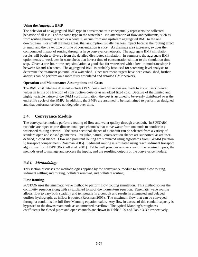
Using the Aggregate BMP The behavior of an aggregated BMP typ e in a treatment train c onceptually represents the collected behavior of all B MPs of the same type in the watershed. No attenuation of flow and pollutants, such as from routin g through a reach or a conduit, occurs fro m one upstream aggregated BMP to the one downstream. For small drainage areas, that assumption usually has less impact because the routing effect is small and the travel time or time of co ncentration is short. As drainage area increases, so does the compounded impac t of routing through a large conveyance network. The aggregate BMP simulation results will begin to diverge from the detailed distributed simulation. In summary, the aggregate BMP option tends to work best in watersheds t hat have a time of concentration similar to the simulation time step. Given a one-hour time step simulation, a good size for watershed with a low- to moderate slope is between 50 and 150 acres. The aggregated BMP is probably best used for screening-level analysis to determine the tre atment potential of a watershed. Once treatment targets have been established, further analysis can be perform on a more full y articulated and detailed BMP network.

Operation and Maintenance Assumpt ions and Costs The BMP cost database does not include O&M costs , and provisions are made to allow users to enter values in terms of a fraction o f construction costs or as an added fixed cost. Because of the limited and highly variable nature of th e O&M cost information, the cost is assumed to be evenly distributed over the entire life cycle of the BMP. In addition, the BMPs are assumed to be maintained to perform as designed and that performance does not degrade over time.

3.4. Conveyance Module The conveyance m odule performs routing of flow and water quality through a conduit. In SUSTAIN, conduits are pipes or one-dimensional open channels that move water from one node to another in a watershed routing network. The cross-sectional shapes of a conduit can be selected from a variet y of standard open and closed geometries. Irregular, natural, cross-section shapes are supported, as are user-defined, closed shapes. Flow and pollutant routing are simulated using algorithms from SWMM (ve rsion 5) transport compartment (Rossman 2005). Sediment routing is simulated using reach sediment tran sport algorithms from HSPF (Bicknell et al. 2001). Table 3-28 provides an overview of the required inputs, the methods used to manage and process the inputs, and the resulting outputs of the conveyance module.

3.4.1. Methodology This section discusses the methodologies applied by the conveyance module to handle flow routing, sediment settling and routing, pollutant removal, and pollutant routing.

Flow Routing SUSTAIN uses the kinematic wave method to perform flow routing simulation. This method solves the continuity equation along with a simplified form of the momentum equation. Kinematic wave routing allows flow to vary both spatially and temporally in a conduit and results in attenuated and delayed outflow hydrographs as inflow is routed (Rossman 2005). The maximum flow that can be conveyed through a conduit is the full-flow Manning equation value. Any flow in excess of this conduit capa city is bypassed to t he downstream node as an untreated overflow. The typical Manning’s roughness coefficients for closed pipes and open channels are shown in Table 3-29 and Table 3-30, respectively.

3-74

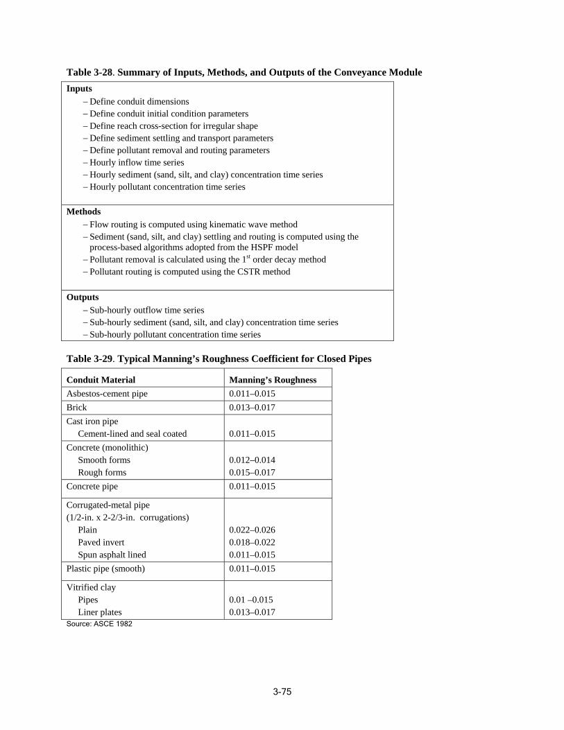
Table 3-28. Summary of Inputs, Methods, and Outputs of the Conveyance Module Inputs

− Define conduit dimensions − Define co it initial condition parameters

efine reach cross-section for irregular shape nsport parameters

− Hourly sediment (sand, silt, and clay) concentration time series

ndu − D − Define sediment settling and tra − Define pollutant removal and routing parameters − Hourly inflow time series

− Hourly pollutant concentration time series

Methods − Flow routing is computed using kinematic wave method

diment (sand, silt, and clay) settling and routing is computed using the opted from the HSPF model

using the 1st order decay method e CSTR method

− Se process-based algorithms ad

− Pollutant removal is calculated − Pollutant routing is computed using th

Outputs ow time series − Sub-hourly outfl

− Sub-hourly sediment (sand, silt, and clay) concentration time series − Sub-hourly pollutant concentration time series

Table 3-29. Typical Manning’s Roughness Coefficient for Closed Pipes

Conduit Material Manning’s Roughness Asbestos-cement pipe 0.011–0.015 Brick 0.013–0.017 Cast iron pipe

Cement-lined and seal coated 0.011–0.015 Concrete (monolithic)

Smooth forms Rough forms

0.012–0.014 0.015–0.017

Concrete pipe 0.011–0.015

Corrugated-metal pipe (1/2-in. x 2-2/3-in. corrugations)

Plain Paved invert Spun asphalt lined

0.022–0.0260.018–0.0220.011–0.015

Plastic pipe (smooth) 0.011–0.015

Vitrified clay Pipes Liner plates

0.01 –0.015 0.013–0.017

Source: ASCE 1982

3-75

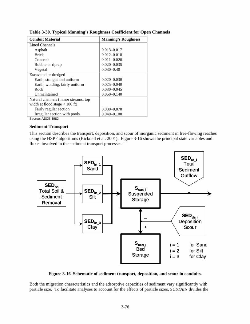
Table 3-30. Typical Manning’s Roughness Coefficient for Open Channels Conduit Material Manning’s Roughness Lined Channels

Asphalt 0.013–0.017 Brick 0.012–0.018

Concrete 0.011–0.020 Rubble or riprap 0.020–0.035 Vegetal 0.030–0.40

Excavated or dredged Earth, straight and uniform 0.020–0.030 Earth, winding, fairly uniform 0.025–0.040 Rock 0.030–0.045

Unmaintained 0.050–0.140 Natural channels (minor streams, top width at flood stage < 100 ft)

Fairly regular section 0.030–0.070 Irregular section with pools 0.040–0.100

Source: ASCE 1982

Sediment Transport This section describes the transport, deposition, and scour of inorganic sediment in free-flowing reaches using the HSPF algorithms (Bicknell et al. 2001). Figure 3-16 shows the principal state variables and fluxes involved in the sediment transport processes.

SESEDDroro__iiSESEDDinin_1_1 ToTottaall SSandand SSeedidimmeentnt

OuOutfltflooww

SESEDDsoso SSsususs_i_iTTootatal Sl Sooilil && SESEDDinin_2_2 SSususppendeendeddSSeedidimmeentnt SiSiltlt SSttororagageeReRemmoovvaall

__ SESEDDdsds__ii DDeposeposiittiioonnSESEDDinin_3_3

ClaClayy Sc+ Sc+ oouurr

SSbebed_d_ii ii == 11 fforor SSandand BeBedd i =i = 22 ffoorr SSiilltt

SSttororagagee ii == 33 fforor CCllayay

Figure 3-16. Schematic of sediment transport, deposition, and scour in conduits.

Both the migration characteristics and the adsorptive capacities of sediment vary significantly with particle size. To facilitate analyses to account for the effects of particle sizes, SUSTAIN divides the

3-76

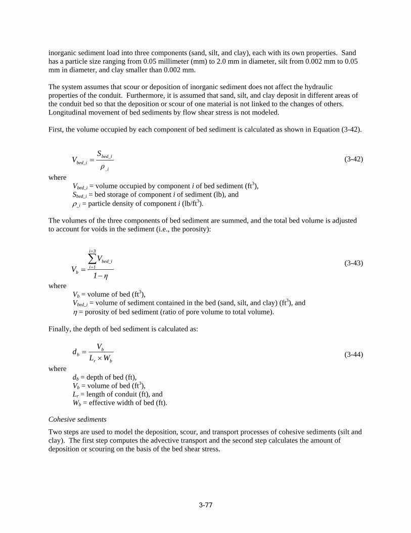
inorganic sediment load into three components (sand, silt, and clay), each with its own properties. Sand has a particle size ranging from 0.05 millimeter (mm) to 2.0 mm in diameter, silt from 0.002 mm to 0.05 mm in diameter, and clay smaller than 0.002 mm.

The system assumes that scour or deposition of inorganic sediment does not affect the hydraulic properties of the conduit. Furthermore, it is assumed that sand, silt, and clay deposit in different areas of the conduit bed so that the deposition or scour of one material is not linked to the changes of others. Longitudinal movement of bed sediments by flow shear stress is not modeled.

First, the volume occupied by each component of bed sediment is calculated as shown in Equation (3-42).

Sbed_iV = (3-42)bed_i ρ_i

where Vbed_i = volume occupied by component i of bed sediment (ft3), Sbed_i = bed storage of component i of sediment (lb), and ρ_i = particle density of component i (lb/ft3).

The volumes of the three components of bed sediment are summed, and the total bed volume is adjusted to account for voids in the sediment (i.e., the porosit y):

i=3

∑Vbed_i (3-43)i=1Vb = 1− η

where Vb = volume of bed (ft3), Vbed_i = volume of sediment contained in the bed (sand, silt, and clay) (ft3), and η = porosity of bed sediment (ratio of pore volume to total volume).

Finally, the depth of bed sediment is calculated as:

Vbd = b (3-44)Lr ×Wb

where db = depth of bed (ft), Vb = volume of bed (ft3), Lr = length of conduit (ft), and Wb = effective width of bed (ft).

Cohesive sediments

Two steps are used to model the deposition, scour, and transport processes of cohesive sediments (silt and clay). The first step computes the advective transport and the second step calculates the amount of deposition or scouring on the basis of the bed shear stress.

3-77

Advective Transport of Constituent This section computes the concentration of material in a conduit and the quantities of material that leave the conduit due to longitudinal advection. Two assumptions are made in the solution technique for normal advection: each constituent is uniformly dispersed throughout the waters of the conduit and is completely entrained by the flow—that is, the material moves at the same horizontal velocity as the w ater.

The equation of continuity can be written as:

SEDin − SEDro = (C ×V ) − (Cs ×V s ) (3-45)where

SEDin = total inflow of sediment over the interval (lb), SEDro = total outflow of sediment over the interval (lb),

C 3s = sediment concentration at the start of the interval (lb/ft ),

C = sediment concentration at the end of the interval (lb/ft3), Vs = volume of water stored at the start of the interval (ft3), and V = volume of water stored at the end of the interval (ft3).

The other basic equation states that the total outflow of material o ver the time interval is a weighted mean of two estimates; one based on conditions at the start of the interval, the other on ending conditions:

SED ro = (C s ×Q s × js)+ (C ×Q × cojs ) (3-46)where

Qs = outflow rate at the start of the interval (ft3/time interval), Q = outflow rate at the end of the interval (ft3/time interval), js = weighting factor, and cojs = 1 – js.

By combining Equations (3-45) and (3-46) we can solve fo r the concentration C:

SED + C × (V − Q × js)in s s sC = (3-47)

V + Q × cojs

The total amount of material leaving the conduit during the interval is calculated using Equation (3-46). If the conduit goes dry during the interval, the total amount of material leaving the conduit is the sum of the material coming in and the material leaving based on the concentration at the start of the interval:

SEDro = SEDin + (Cs ×Qs × js) (3-48)

Deposition and Scouring Exchange of cohesive sediments with the bed is dependent upon the shear stress exerted on the bed surface. When the shear stress (τ ) in the conduit is less than the user-supplied, critical, shear stress for deposition (τcd), sediment deposition occurs. On the other hand, when the shear stress is greater than the user-supplied, critical, shear stress for scour (τcs), scouring of cohesive bed sediments takes place. The rate of deposition for a particular fraction of cohesive sediment is bas ed on a simplification of Krone’s (1962) equation in the following form:

3-78

⎛ τ ⎞

D = ω×C × 1− (3-49)⎜⎜ τ ⎟⎟

⎝ cd ⎠

where D = rate at which sediment settles out of suspension (lb/ft2 interval), ω = settling velocity for cohesive sediment (ft/interval), C = concentration of suspended sediment (lb/ft3), τ = shear stress (lb/ft2), and τcd = critical shear stress for deposition (lb/ft2).

The rate of change of suspended sediment concentration in the conduit due to deposition can be expressed as:

dC D

= − (3-50)dt dav

where dav = average depth of water in the conduit (ft).

By substituting the expression for deposition rate (D) from Equation (3-49), and integrating and rearranging Equation (3-50), a solution can be obtained for the concentration of suspended sediment lo st to deposition during a simulation interval (Cdep):

⎡ ⎧⎛ ω ⎞ ⎛ τ ⎞⎫⎤

Cdep = C × ⎢1− exp⎨⎜⎜− ⎟⎟×⎜⎜1− ⎟⎟⎬⎥ (3-51)d τ⎢⎣ ⎩⎝ av ⎠ ⎝ cd ⎠⎭⎦⎥

where C = concentration of suspended sediment at the start of interval (lb/ft3), ω = settling velocity for sediment fraction (ft/interval), dav = average depth of water in conduit (ft), τ = shear stress (lb/ft2), and τcd = critical she ar stress for deposition (lb/ft2).

The user must supp ly value s for settling velocity (ω) and critical sh ear stress for deposition (τcd) for silt and clay fractions in cohesive sedime nt.

The amount of sed imen t in suspension (Ssus) is updated by subtracting the amount settled. Likewise, the amount of sediment in bed (Sbed) is updated by adding the amount settled on it.

The rate of resuspension, or scour, of cohesive sediments from the bed is derived from a modified form o f Partheniades’ (1962) equation:

⎛ τ ⎞

S = µ ×⎜⎜ − 1⎟⎟ (3-52) ⎝ τcs ⎠

where S = rate at which sediment is scoured from the bed (lb/ft2 interval),

3-79

µ = erodibility coefficient for the sediment fraction (lb/ft2 interval), and τcs = critical shear stress for scour (lb/ft2).

The rate of change of suspended sediment fraction concentration in the conduit due to scour can be expressed as:

dC S

= − (3-53)dt dav

By substituting the expression for scour rate (S) from Equation (3-52) and integrating and rearranging Equation (3-53), a solution can be obtained for the concentration of suspended sediment added to suspension by scour during a simulation interval (Cscr):

µ ⎡ τ ⎤

C = × −1 (3-54)scr ⎢ ⎥d τav ⎣ cs ⎦

where µ = erodibility coefficient (lb/ft2 interval), and dav = average depth of water (ft).

The user is required to supply values for the erodibility coefficient (µ) and critical shear stress for scour (τcs) for each fraction of cohesive sediment (silt and clay) that is modeled.

The amount of sediment in suspension (Ssus) is updated by adding the scoured mass, as is the amoun t of sediment in bed (Sbed) by subtracting the scoured mass.

If the amount of scoured sediment is greater than the original sediment in the bed, all sediment in the bed will be resuspended and the amount of sediment in the bed is set to zero.

Non-cohesive Sediment

Erosion and deposition of sand, or non-cohesive sediment, is affected by the amount of sediment tha t the flow is capable of carrying. If the amount of sand being transported is less than the flow can carry for the hydrodynamic conditions of the conduit, sand is scoured from the bed. This occurs until the actual sand transport rate becomes equal to the carrying capacity of the flow or until the available bed sand is all scoured. Conversely, deposition occurs if the sand transport rate exceeds the flow’s carrying capac ity.

The sand transport capacity for a conduit is calculated by using an input power function of the velocity. The potential sand concentration (Cp) is determined by the following conversion:

C p = k × υav j (3-55)

where Cp = potential sand concentration (lb/ft3), k = coefficient in the sandload suspension equation (input parameter), j = exponent in sandload suspension equation (input parameter), and υav = average velocity (ft/s).

3-80

SED + SED + C × (V − Q × js)in ds s s sC = (3-58)

V + Q × cojs

The potential outflow of sand (SEDpro) is calculated as:

SED pro = (Cs ×Qs × js)+ (Cp ×Q × cojs) (3-56)

where Cs, Qs, js, Q, and cojs are as previously defined for Equations (3-45) and (3-46).

The potential scour from, or deposition to, the bed storage is found using the continuity equation:

SEDpds = (V × C p )− (Vs × Cs )+ SEDpro − SEDin (3-57)

where SEDpds = potential scour (+) or deposition (-) (lb), Cp = potential sand concentration at the end of the interval (lb/ft3), Cs = sand concentration at the start of the interval (lb/ft3), SEDpro = potential outflow of sand over the interval (lb), and SEDin = inflow of sand during the interval (lb).

The potential scour is compared to the amount of available sand for resuspension. If scouring potential is less than the available sands, the demand is satisfied i n full and the bed storage is adjusted accordingly. If the potential scour cannot be satisfied by bed storage, all the available bed sand is suspended, and the bed storage is exhausted. The concentration of suspended sand (C) is calculated as:

where C = concentration of sand at end of interval (lb/ft3), Cs = concentration of sand at start of interval (lb/ft3), SEDin = inflow of sand during the interval (lb), and SEDds = sand scoured from, or deposited to, the bottom (lb).

The total amount of sand leaving the conduit during the interval is calculated using Equation (3-58). If a conduit goes dry during an interval, or if there is no outflow from the conduit, all the sand in suspension at the beginning of the interval is assumed to settle out, and the bed storage is correspondingly increased.

Sediment Transport Input Parameters

Parametric information required for silt and clay includes particle diameter (φ), particle settling velocity in still water (ω), particle density (ρ), critical shear stress for deposition (τcd), critical shear stress for scour (τcs), and erodibility coefficient (µ). Parameter values required for sand include median bed sediment diameter (φ50) and particle settling velocity (ω). Table 3-31 shows the range of input parameters that are recommended.

Sediment Transport Calibration

Sediment transport parameters are typically derived by calibration. The calibration process involves establishing initial parameter values and a subsequent adjustment process. The eroded material from each land use category is fractionated into sand, silt, and clay before entering a conduit using available soils information; typically, a single fractionation scheme is used for all conduits. The fraction should reflect the relative percent of the surface material (i.e., sand, silt, clay) available for input to the conduit.

3-81

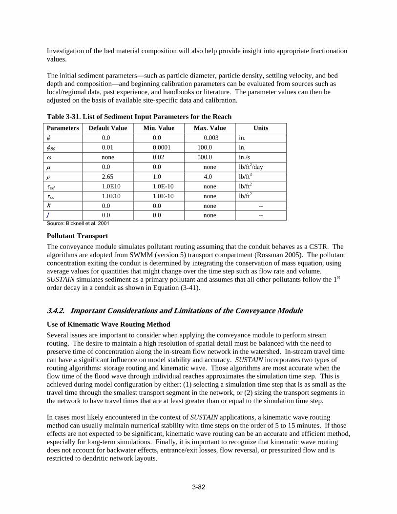
Investigation of the bed material composition will also help provide insight into appropriate fractionation values.

The initial sediment parameters—such as particle diameter, particle density, settling velocity, and bed depth and composition—and beginning calibration parameters can be evaluated from sources such as local/regional data, past experience, and handbooks or literature. The parameter values can then be adjusted on the basis of available site-specific data and calibration.

Table 3-31. List of Sediment Input Parameters for the Reach Parameters Default Value Min. Value Max. Value Units φ 0.0 0.0 0.003 in. φ50 0.01 0.0001 100.0 in. ω none 0.02 500.0 in./s µ 0.0 0.0 none lb/ft2/day ρ 2.65 1.0 4.0 lb/ft3

τcd 1.0E10 1.0E-10 none lb/ft2

τcs 1.0E10 1.0E-10 none lb/ft2

k 0.0 0.0 none --j 0.0 0.0 none --Source: Bicknell et al. 2001

Pollutant Transport The conveyance module simulates pollutant routing assuming that the conduit behaves as a CSTR. The algorithms are adopted from SWMM (version 5) transport compartment (Rossman 2005). The pollutant concentration exiting the conduit is determined by integrating the conservation of mass equation, using average values for quantities that might change over the time step such as flow rate and volume. SUSTAIN simulates sediment as a primary pollutant and assumes that all other pollutants follow the 1st

order decay in a conduit as shown in Equation (3-41).

3.4.2. Important Considerations and Limitations of the Conveyance Module Use of Kinematic Wave Routing Method Several issues are important to consider when applying the conveyance module to perform stream routing. The desire to maintain a high resolution of spatial detail must be balanced with the need to preserve time of concentration along the in-stream flow network in the watershed. In-stream travel time can have a significant influence on model stability and accuracy. SUSTAIN incorporates two types of routing algorithms: storage routing and kinematic wave. Those algorithms are most accurate when the flow time of the flood wave through individual reaches approximates the simulation time step. This is achieved during model configuration by either: (1) selecting a simulation time step that is as small as the travel time through the smallest transport segment in the network, or (2) sizing the transport segments in the network to have travel times that are at least greater than or equal to the simulation time step.

In cases most likely encountered in the context of SUSTAIN applications, a kinematic wave routing method can usually maintain numerical stability with time steps on the order of 5 to 15 minutes. If those effects are not expected to be significant, kinematic wave routing can be an accurate and efficient method, especially for long-term simulations. Finally, it is important to recognize that kinematic wave routing does not account for backwater effects, entrance/exit losses, flow reversal, or pressurized flow and is restricted to dendritic network layouts.

3-82

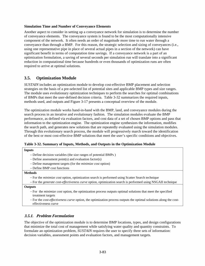
Simulation Time and Number of Conveyance Elements Another aspect to consider in setting up a conveyance network for simulation is to determine the number of conveyance elements. The conveyance system is found to be the most computationally intensive component of t he network. It often needs an order of magnitude more time to run water through a conveyance than through a BMP. For this reason, the strategic selection and sizing of conve yances (i.e., using one representative pipe in place of several actual pi pes in a section of the net work) can have significant benefit in terms of computation time savings. If a conveyance network is a part of an optimization for mulation, a saving of several seconds per simulation run will translate into a significant reduction in com putational time because hundreds or eve n thousands of optimization runs are often required to arrive at optimal solutions.

3.5. Optimization Module SUSTAIN includes an optimization module to develop cost-effective BMP placement and selection strategies on the basis of a pre-selected list of potential sites and applicable BMP types and size ranges. The module use s evolutionary optimiza tion techniques to perform the sear ches for optimal combinations of BMPs that meet the user-defined decision criteria. Table 3-32 summari zes the r equired inputs, methods used, and outputs and Figure 3-17 presents a conceptual overview of the mod ule.

The optimization module works hand-in-hand with the BMP, land, and conveyanc e modules during the search process in an iterative and evolutionary fashion. The simulation mo dules evaluate the BMP performance, as d efined via evaluation factors, and cost data of a set of chosen BMP options and pass that information to t he optimization engine. The optimiza tion engine synthesizes the information, modifies the search path, a nd generates new solutions that are repe atedly evaluated using th e sim ulation modules. Through this e volutionary search process, the module will progressiv ely march t oward the identification of the best or most cost-effective BMP solutions th at meet the user’s specific conditions and objectives.

Table 3-32. Summary of Inputs, Met hods, and Outputs in the Optimizatio n Module Inputs

− Define decisi s ion factor(s)

ana ) − Define BMP

on variables (the size ranges of potential BMPs ) − Define asse − Define m

sment point(s) and evaluat gement targets (for the minimize cost option cost functions

Methods − For − For the g

the mini rmed using Scatte echn ene s perf ng technique

mize cost option, optimization search is perfo r Search t ique NSGAII rate cost-effectiveness curve option, optimization search i ormed usi

Outputs − For the minimize cost option, the optimization process outputs optimal solutions that meet the specified

treatment targets − For the cost-effectiveness curve option, the optimization process outputs the optimal solutions along the cost-

effectiveness curve

3.5.1. Problem Formulation The objective of the optimization module is to determine BMP locations, types, and design co nfigurations that minimize the total cost of management while satisfying water quality and quantity constraints. To formulate an optimization problem, SUSTAIN requires the user to specify three sets of information: decision variables, assessment points and evaluation factors, and management targets.

3-83

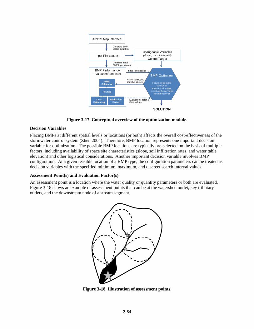
ArcGIS Map Interface

Input File Loader

BMP Performance Evaluation/Simulator

BMP Calculator

Changeable Variables (#, min, max, increment)

Control Target Generate Initial BMP Input Values

Generate BMP Model Input File

Routing

Cost Estimating

Evaluation Factor

SOLUTION

Evaluation Factor & Cost Values

Initial Run Results:

New ChangeableVariable Values

BMP Optimizer

Feed new possible solution to

evaluator/simulator based on the previous

simulation result

Figure 3-17. Conceptual overview of the optimization module.

Decision Variables Placing BMPs at different spatial levels or locations (or both) affects the overall cost-effectiveness of the stormwater control system (Zhen 2004). Therefore, BMP location represents one important decision variable for optimization. The possible BMP locations are typically pre-selected on the basis of multi ple factors, including availability of space site characteristics (slope, soil infiltration rates, and water table elevation) and other logistical considerations. Another important decision variable involves BMP configuration. At a given feasible location of a BMP type, the configuration parameters can be treated a s decision variables with the specified minimum, maximum, and discreet search interval values.

Assessment Point(s) and Evaluation Factor(s) An assessment point is a location where the water quality or quantity parameters or both are evaluated. Figure 3-18 shows an example of assessment points that can be at the watershed outlet, key tributary outlets, and the downstream node of a stream segment.

Figure 3-18. Illustration of assessment points.

3-84

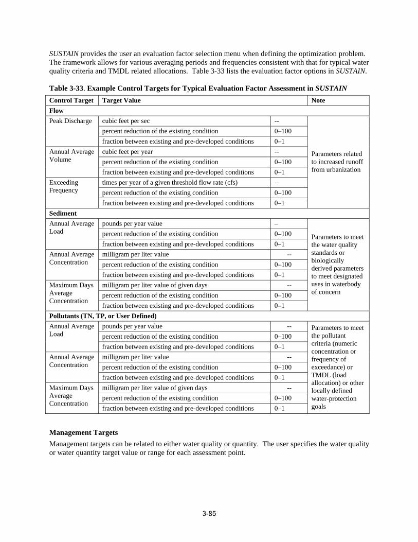
SUSTAIN provides the user an evaluation factor selection menu when defining the optimization problem. The framework allows for various averaging periods and frequencies consistent with that for typica l water quality criteria and TMDL related allocations. Table 3-33 lists the evaluation factor options in SUSTAIN.

Table 3-33. Example Control Targets for Typical Evaluation Factor Assessment in SUSTAIN Control Target Target Value Note Flow Peak Discharge cubic feet per sec --

Parameters related to increased runoff from urbanization

percent reduction of the existing condition 0–100 fraction between existing and pre-developed conditions 0–1

Annual Average Volume

cubic feet per year --percent reduction of the existing condition 0–100 fraction between existing and pre-developed conditions 0–1

Exceeding Frequency

times per year of a given threshold flow rate (cfs) --percent reduction of the existing condition 0–100 fraction between existing and pre-developed conditions 0–1

Sediment Annual Average Load

pounds per year value –

biologically derived parameters to meet designated uses in waterbody

Parameters to meet ality

standards or

of concern

the water qu percent reduction of the existing condition 0–100 fraction between existing and pre-developed conditions 0–1

Annual Average Concentration

milligram per liter value --percent reduction of the existing condition 0–100 fraction between existing and pre-developed conditions 0–1

Maximum Days Average Concentration

milligram per liter value of given days --percent reduction of the existing condition 0–100 fraction between existing and pre-developed conditions 0–1

Pollutants (TN, TP, or User Defined) Annual Average Load

pounds per year value -­ Parameters to meet the pollutant

or

allocation) or other locally defined water-protection

criteria (numeric concentration frequency of exceedance) or TMDL (load

goals

percent reduction of the existing condition 0–100 fraction between existing and pre-developed conditions 0–1

Annual Average Concentration

milligram per liter value --percent reduction of the existing condition 0–100 fraction between existing and pre-developed conditions 0–1

Maximum Days Average Concentration

milligram per liter value of given days --percent reduction of the existing condition 0–100 fraction between existing and pre-developed conditions 0–1

Management Targets Management targets can be related to either water quality or quantity. The user specifies the water quality or water quantity target value or range for each assessment point.

3-85

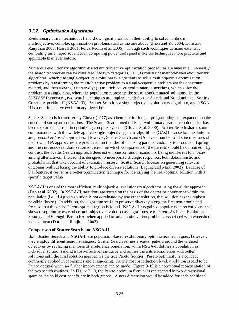
3.5.2. Optimization Algorithms Evolutionary search techniques have shown great promise in their ability to solve nonlinear, multiobjective, complex optimization problems such as the one above (Zhen and Yu 2004; Dorn and Ranjithan 2003; Harrell 2001; Perez-Pedini et al. 2005). Though such techniques demand extensive computing time, rapid advances in computing power and speed make the techniques more practical and applicable than ever before.

Numerous evolutionary algorithm-based multiobjective optimiz ation procedures are available. Generally, the search techniques can be classified into two categories, i.e., (1) constraint method-based evolutionary algorithms, which u se single-objective evolutionary algorithms to solve multiobjective optimization problems by transfo rming the multiobjective problem to a single-objective problem via the constraint method, and then so lving it iteratively; (2) multiobjective evolutionary algorithms, which solve the problem in a single pass, where the population represents the set of nondominated solutions. In the SUSTAIN framework, two search techniques are implemented: Scatter Search and Nondominated Sorting Genetic Algorithm-II (NSGA-II)). Scatter Search is a single-ojective evolutionary algorithm, and NSGA­II is a multiobjective e volutionary algorithm.

Scatter Search is introduced by Glover (1977) as a heuristic for integer programming that expanded o n the concept of surrogate constraints. The Scatter Search method is an evolutionary search technique that has been explored and used in optimizing complex systems (Glover et al. 2000). Scatter Search shares some commonalties with the widely applied single-objective genetic algorithms (GAs) because both techniques are population-based approaches. However, Sca tter Search and GA have a number of distinct features of their own. GA approaches are predicated on the idea of choosing parents randomly to produce offspring and then introduce randomization to determine which components of the parents should be combined. By contrast, the Scatter Search approach does not emphasize randomization or being indifferent to choices among alternatives. Instead, it is designed to incorporate strat egic responses, both deterministic and probabilistic, that take account of evaluation history. Scatter Search focuses on generating relevant outcomes without losing the ability to produce diverse solutio ns (Laguna and Marti 2002). Because of that feature, it serves as a better optimization technique for identif ying the near-optimal solution with a specific target value.

NSGA-II is one of the most efficient, multiobjective, evolutionary algorithms using the elitist approach (Deb et al. 2002). In NSGA-II, solutions are sorted on the basis of the degree of dominance within the population (i.e., if a given solution is not dominated by any other solution, that solution has the highest possible fitness). In addition, the algorithm seeks to preserve diversity along the first non-dominated front so that the entire Pareto-optimal region is found. NSGA-II has gained popularity in recent years and showed superiority over ot her multiobjective evolutionary algorithms, e.g. Pareto-Archived Evolution Strategy and Strength-Pareto EA, when applied to solve optimization problems associated with watershed management (Dorn and Ranjithan 2003).

Comparison of Scatter Search and NSGA-II Both Scatter Search and NSGA-II are population-based evolutionary optimization techniques; however, they employ different search strategies. Scatter Search refines a scatter pattern around the targeted objectives by replacing members of a reference population, while NSGA-II defines a population a s individual solutions along a cost-effectiveness curve and refines the entire population with better solutions until the final solution approaches the true Pareto frontier. Pareto optimality is a concept commonly applied in economics and engineering. At any cost or reduction level, a solution is said to be Pareto optimal when no further improvements can be made. Figure 3-19 is a conceptual representation o f the two search routines. In Figure 3-19, the Pareto optimum frontier is represented in two-dimensional space as the solid cost-benefit arc in both graphs. A new dimension would be added for each additional

3-86

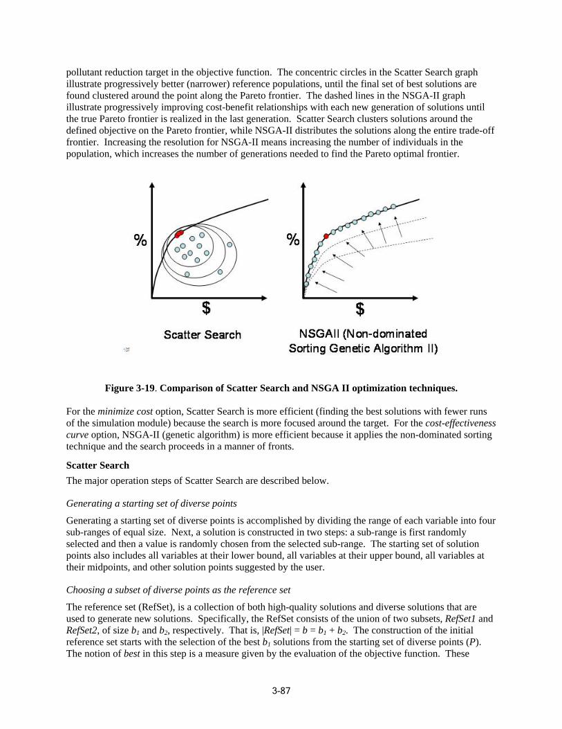
pollutant reduction target in the objective function. The concentric circles in the Scatter Search graph illustrate progressively better (narrower) reference populations, until the final set of best solutions are found clustered around the point along the Pareto frontier. The dashed lines in the NSGA-II graph illustrate progressively improving cost-benefit relationships with each new generation of solutions until the true Pareto frontier is realized in the last generation. Scatter Search clusters solutions around the defined objective on the Pareto frontier, while NSGA-II distributes the solutions along the entire trade-off frontier. Increasing the resolution for NSGA-II means increasing the number of individuals in the population, which increases the number of generations needed to find the Pareto optimal frontie r.

Figure 3-19. Comparison of Scatter Search and NSGA II optimization techniques.

For the minimize cost option, Scatter Search is more efficient (finding the best solutions with fewer runs of the simulation module) because the search is more focused around the target. For the cost-effectiveness curve option, NSGA -II (genetic algorithm) is more efficient because it applies the non-dominated sorting technique and the search proceeds in a manner of fronts.

Scatter Search The major operation steps of Scatter Search are described below.

Generating a starting set of diverse points

Generating a starting set of diverse points is accomplished by dividing the range of each variable into four sub-ranges of equal size. Next, a solution is constructed in two steps: a sub-range is first randomly selected and then a value is randomly chosen from the selected sub-range. The starting set of solution points also includes all variables at their lower bound, all variables at their upper bound, all variables at their midpoints, and other solution points suggested by the user.

Choosing a subset of diverse points as the reference set

The reference set (RefSet), is a collection of both high-quality solutions and diverse solutions that are used to generate new s olutions. Specifically, the RefSet consists of the union of two subsets, RefSet1 and RefSet2, of size b1 and b2, respectively. That is, |RefSet| = b = b1 + b2. The construction of the initial reference set starts with the selection of the best b1 solutions from the starting set of diverse po ints (P). The notion of best in this step is a measure given by the evaluation of the objective function. These

3-87

solutions are added to RefSet and deleted from P. For each improved solution in P – RefSet, the minimum of the Euclidean distances to the solutions in RefSet is computed. Euclidean distance is the straight line distance between two points. For example, in a two-dimensional plane, the Euclidean distance is the straight line between point 1 at (x1, y1) and point 2 at (x2, y2) and is equal to (x - x ) ² + (y - y ) ² .1 2 1 2

Then, the solution with the maximum of these minimum distances is selected. This solution is added to RefSet and deleted from P and the minimum distances are updated. This process is repeated b2 times. The resulting reference set has b1 high-quality solutions and b2 diverse solutions.

Starting the search for the optimal solution by using a linear combination method to construct new solution points from the reference solution points

The linear combination is based on the three types of formulation, in which x′ and x″ are reference solution points, and x1–3 is the newly generated solution points:

x1 = x′ – d x2 = x″ – d x3 = x′ + d

where and r is a random number in the range of (0, 1).

Updating the RefSet

In the course of searching for a global optimum, the RefSet is continuously updated. The solutions having better quality, or ones that can improve the diversity of the reference set, replace the old points in the set.

Stop the search if the stopping criteria are met

The stopping criteria can be defined, at the user’s option, either as the maximum number of itera tion runs, or the minimum improvement between updates of the reference set, or both, in which case, the search process will be stopped when either of the criteria is met.

NSGA-II The major operation steps of NSGA-II are described below.

Creation of first generation

When applying the NSGA-II, a random parent population (P0) consisting of N solutions is first created. The population is then sorted by the non-dominant level. A solution x(1) is non-dominant to another solution when x(1) performs no worse than the other solution in all objectives, and x(1) performs better than the other solution in at least one objective. At the end of the sorting, each solution is assigned a fitnes s (or rank) equal to its non-dominant level, with a smaller value indicating that the solution is dominated by fewer other solutions.

The processes of tournament selection, crossover, and mutation are used to create a child population (Q0), which has a same size of P0 with N solutions.

x" − x'

d = r 2

3-88

Main loop

In the first step of the main loop, the parent population and the child population are combined (R0). The population of R0 will have 2N solutions. The 2N solutions in R0 are then sorted according to non-domination. Elitism is ensured in this step because both the parent and the child population are used in the sorting. The sorted 2N solutions will form various best non-dominated subsets (in which all the solutions are non-dominant to each other, but overall they dominate other subsets). The first N solutions from the ranked best non-dominant subsets, F1,…, Fi, are then selected to form a new parent population (P1). The new parent population is used to create a new child population (O1), and the process continues until the stopping criteria are met.

The NSGA-II uses the crowding distance (the size of the largest cuboid enclosing solution x(1) without including any other solution in the population) concept to maintain solution diversity. That is, in cases where two solutions have the same non-domination rank, the solution with larger crowding distance is always preferred.

Stopping criteria

The user can make the NSGA-II stop when the new parent population does not ch ange for two consecutive loops. The stopping criterion can also be that the fitness function does not improve after a certain numbe r of iterations.

Optimization Options SUSTAIN provides two optimization options: (1) cost minimization, and (2) cost-effectiveness curve. In the cost-minimization option, the optimization search process identifies the near-optimal solutions that meet the user-specified management targets. With the cost-effectiveness curve option, the optimization process reveals all the cost-effective solutions within the user-specified management target range.

Cost-Minimization Option

With the objective of minimizing cost subject to desired water quality or water quantity objectives (or both) at a specified location (assessment point), the optimization problem formulation can be mathematically expressed as below. In the formulation, a group of BMPi (i = 1,…, n) forms the decision matrix, which defines the optimization engine’s search domain. For each potential location, the user defines the feasible range of BMP type and configura tion parameters.

The objective is to:

Minimize n

∑Cost(BMPi ) i=1

subject to: Qj ≤ Qmaxj and

Lk ≤ Lmaxk where

BMPi = a set of BMP configuration decision variables assoc iated with location i, Qj = the computed amount of water quantity factor at the assessment poi nt j, Qmaxj =the maximum value of the water qua ntity factor targeted at the assessment point j, Lk = the computed amount of water quality loading factor at the assessment point k, and Lmaxk = the maximum value of the water quality loading targeted at the assessment point k.

3-89

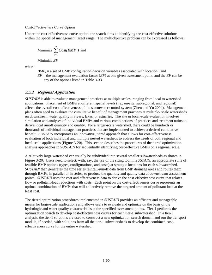
Cost-Effectiveness Curve Option

Under the cost-effectiveness curve option, the search aims at identifying the cost-effective solutions within the specified management target range. The multiobjective problem can be expressed as fol lows:

Minimize

Minimize EF

n

∑Cost(BMPi ) and i=1

where BMPi = a set of BMP configuration decision variables associated with location i and EF = the management evaluation factor (EF) at one given assessment point, and the EF can be

any of the options listed in Table 3-33.

3.5.3. Regional Application SUSTAIN is able to evaluate management practices at multiple scales, ranging from local to watershed applications. Placement of BMPs at different spatial levels (i.e., on-site, subregional, and regional) affects the overall cost-effectiveness of the stormwater control system (Zhen and Yu 2004). Management plans often need to evaluate the cumulative benefit of manage ment practices at multiple- scale watersheds on downstream water quality in rivers, lakes, or estuaries. The site or local-scale evaluation involves simulation and analyses of individual BMPs and various combinations of practices and treatment train s to derive local runoff quantity and quality. For a larger-scale watershed, there could be hundreds or thousands of individual management practices that are implemented to achieve a desired cumulative benefit. SUSTAIN incorporates an innovative, tiered approach that allows for cost-effectiveness evaluation of both individual and multiple nested watersheds to address the needs of both regional an d local-scale applications (Figure 3-20). This section describes the procedures of the tiered optimization analysis approaches in SUSTAIN for sequentially identifying cost-effective BMPs on a regional scale.

A relatively large watershed can usually be subdivided into several smaller subwatersheds as shown in Figure 3-20. Users need to select, with, say, the use of the siting tool in SUSTAIN, an appropriate suite o f feasible BMP options (types, configurations, and costs) at strategic locations for each subwatershed. SUSTAIN then generates the time series rainfall-runoff data from BMP drainage areas and routes them through BMPs, in parallel or in series, to produce the quantity and quality data at downstream assessment points. SUSTAIN uses the cost and effectiveness da ta to derive the cost-effectiveness curve that relates flow or pollutant-load reductions with costs. Each point on the cost-effectiveness curve represents an optimal combination of BMPs that will collectively remove the targeted amount of pollutant load at the least co st.

The tiered optimization procedures implemented in SUSTAIN provides an efficient and manageable means for large-scale applications and allows users to evaluate and optimize on the basis of the hydrologic and water quality characteristics at the specified assessment points. Tier-1 performs the optimization search to develop cost-effectiveness curves for each tier-1 subwatershed. In a tier-2 analysis, the tier-1 solutions are used to construct a new optimization search domain and run the transport module, if needed, with solutions from all the tier-1 subwatersheds to develop the combined cost-effectiveness curve for the entire watershed.

3-90

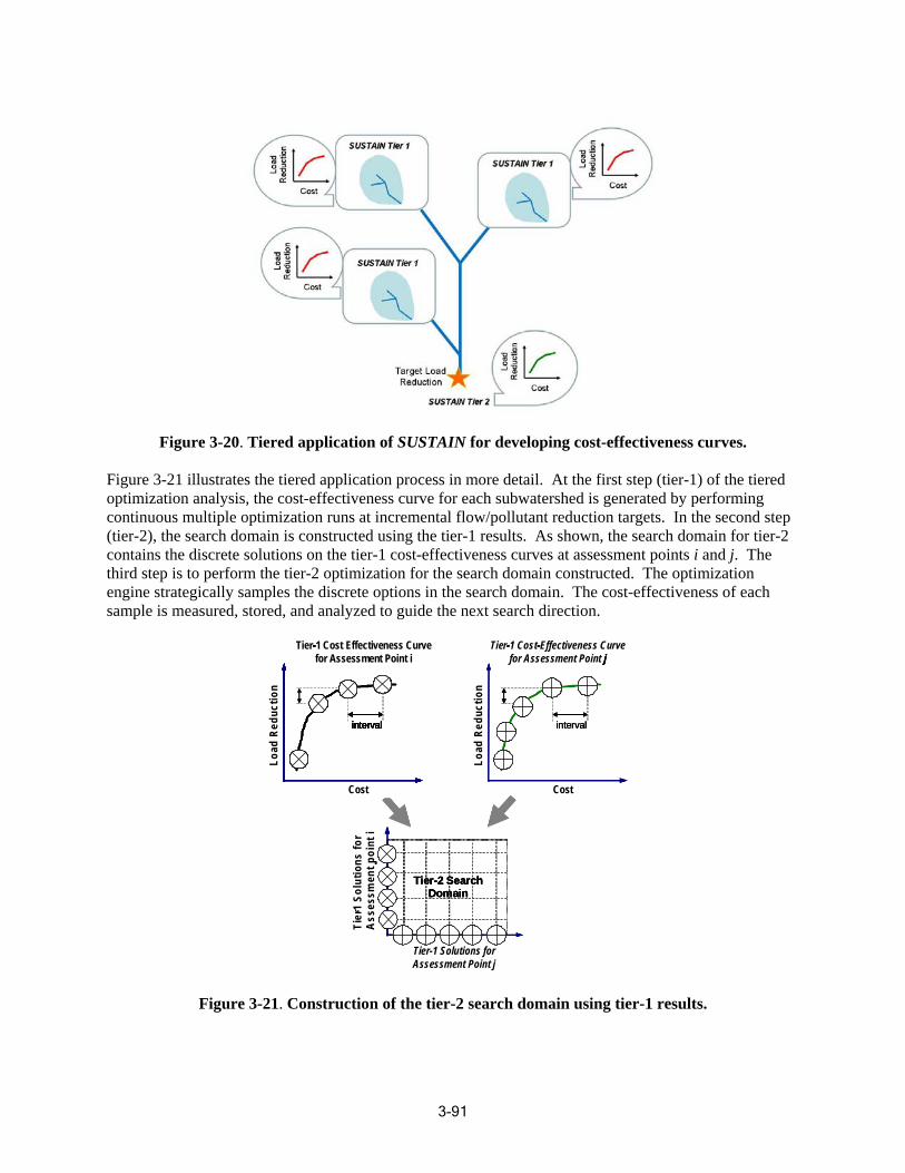
Figure 3-20. Tiered application of SUSTAIN for developing cost-effectiveness curves.

Figure 3-21 illustrates the tiered application process in more detail. At the first step (tier-1) of the tiered optimization analysis, the cost-effectiveness curve for each subwatershed is generated by performing continuous multiple optimization runs at incremental flow/pollutant reduction targets. In the second step (tier-2), the search domain is constructed using the tier-1 results. As shown, the search domain for tier-2 contains the discrete solutions on the tier-1 cost-effectiveness curves at assessment points i and j. The third step is to perform the tier-2 optimization for the search domain constructed. The optimization engine strategically samples the discrete options in the search domain. The cost-effectiveness of each sample is measured, stored, and analyzed to guide the next search direction.

Cost

Load

Red

uctio

n

Cost

Load

Re

uctio

n

Tier-1 Solutions for Assessment Point j

Tier

1 So

lutio

ns fo

r A

sses

smen

toi

nt i

Tier 1 Cost Effectiveness Curve for Assessment Point

Tier 1 Cost ffectiveness Curve for As essment Point i

Cost

Load

Re

uctio

n

Cost

Load

Red

uctio

n

Cost

Load

Red

uctio

n

Tier-1 Solutions for Assessment Point j

Tier

1 So

lutio

ns fo

r A

sses

smen

toi

nt i

Tier 1 Cost Effectiveness Curve for Assessment Point

Tier 1 Cost E fectiveness Curve for Assessment Point i

Cost

Load

Red

uctio

n

Cost

Load

Red

uctio

n

Cost

Load

Red

uctio

n

Tier---1 Cost Effectiveness Curve Tier---1 Cost---Effectiveness Curve

interval interval

p

Tier-2 SearchDomain

j

intervalinterval interval

p

Tier-2 SearchDomain

j

intervalinterval

Cost

Lo ad

Re d

uc tio

n

interval

Tier-1 Solutions for Assessment Point j

Tier-

1 So

lu tio

n s fo

rA

sses

sm en

t poi

nt i

Tier-2 Search Domain

for Assessment Point jfor Assessment Point i

interval

Cost

Lo ad

Re d

uc tio

n

interval

Figure 3-21. Construction of the tier-2 search domain using tier-1 results.

3-91

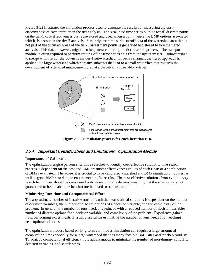
Figure 3-22 illustrates the simulation process used to generate the results for measuring the cost-effectiveness of each iteration in the tier analysis. The simulated time series outputs for all discrete points on the tier-1 cost-effectiveness curve are stored and used when a point, hence the BMP options associated with it, is chosen in the tier-2 analysis. Similarly, the time series runoff data of the watershed area that is not part of the tributary areas of the tier-1 assessment points is generated and stored before the tiered analysis. This data, however, might also be generated during the tier-2 search process. The transport module is often required to perform routing of the time series data from the upstream tier-1 subwatershed to merge with that for the downstream tier-1 subwatershed. In such a manner, the tiered approach is applied to a large watershed which contains subwatersheds or to a small watershed that requires the development of a detailed management plan at a parcel- or a street-block-level.

TM

Channel

r

Tier-1 solution time series at assessment points

are not covered ent points

Time series for the areas/catchment thatby tier-1 assessm

Transport Module:Time Series:

Channel

Conduit

Simulation process for each iteration run:

Tier-1 solution time series at assessment points

are not covered ent points

Time series for the areas/catchment that by tier-1 assessm

Figure 3-22. Simulation process for each iteration run.

3.5.4. Important Considerations and Limitations: Optimization Module Importance of Calibration The optimization engine performs iterative searches to identify cost-effective solutions. The search process is dependent on the cost and BMP treatment effectiveness values of each BMP or a combination of BMPs evaluated. Therefore, it is crucial to have calibrated watershed and BMP simulation modules, as well as good BMP cost data, to ensure meaningful results. The cost-effective solutions from evolutionary search techniques should be considered only near-optimal solutions, meaning that the solutions are not guaranteed to be the absolute best but are believed to be close to it.

Minimizing Run-time and Computational Effort The approximate number of iterative runs to reach the near-optimal solutions is dependent on the number of decision variables, the number of discrete options of a decision variable, and the complexity of the problem. In general, the number of runs needed is reduced with a reduced number of decision variables, number of discrete options for a decision variable, and complexity of the problem. Experience gained from performing experiments is usually useful for estimating the number of runs needed for reaching near-optimal solutions.

The optimization process based on long-term continuous simulation can require a large amount of computation time especially for a large watershed that has many feasible BMP sites and reaches/conduits. To achieve computational efficiency, it is advantageous to minimize the number of non-dummy conduits, decision variables, and search steps.

3-92

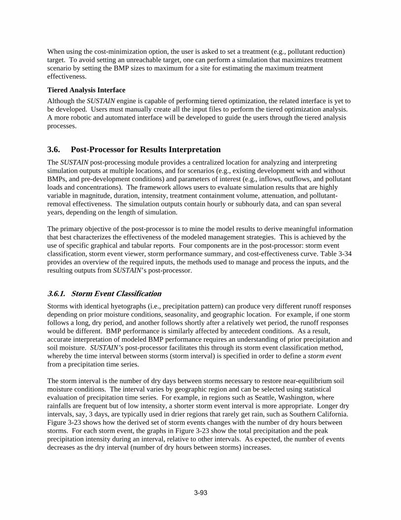
When using the cost-minimization option, the user is asked to set a treatment (e.g., pollutant reduction) target. To avoid setting an unreachable target, one can perform a simulation that maximizes treatment scenario by setting the BMP sizes to maximum for a site for estimating the maximum treatment effectiveness.

Tiered Analysis Interface Although the SUSTAIN engine is capable of performing tiered optimization, the related interface is yet to be developed. Users must manually create all the input files to perform the tiered optimization analysis. A more robotic and automated interface will be developed to guide the users through the tiered analysis processes.

3.6. Post-Processor for Results Interpretation The SUSTAIN post-processing module provides a centralized location for analyzing and interpreting simulation outputs at multiple loc ations, and for scenarios (e.g., existing development with and without BMPs, and pre-development conditions) and parameters of interest (e.g., inflows, outflows, and pollutant loads and concentrations). The framework allows users to evaluate simulation results that are highly variable in magnitude, duration, intensity, treatment containment volume, attenuation, and pollutant-removal effectiveness. The simulation outputs contain hourly or subhourly data, and can span several years, depending on the length of simulation.

The primary objective of the post-processor is to mine the model results to derive meaningful information that best characterizes the effectiveness of the modeled management strategies. This is achieved by the use of specific graphical and tabular reports. Four components are in the post-processor: storm event classification, storm event viewer, storm performance summary, and cost-effectiveness curve. Table 3-3 4 provides an overview of the required inputs, the methods used to manage and process the inputs, and the resulting outputs from SUSTAIN’s post-processor.

3.6.1. Storm Event Classification Storms with identical hyetographs (i.e., precipitation pattern) can produce very different runoff respo nses depending on prior moisture conditions, seasonality, and geographic location. For example, if one storm follows a long, dry period, and another follows shortly afte r a relatively wet period, the runoff responses would be different. BMP performance is similarly affected by antecedent conditions. As a result, accurate interpretation of modeled BMP performance requires an understanding of prior precipitation and soil moisture. SUSTAIN’s post-processor facilitates this through its storm event classification method, whereby the time interval between storms (storm interval) is specified in order to define a storm event from a precipitation time series.

The storm interval is the number of dry days between storms necessary to restore near-equilibrium soil moisture conditions. The interval varies by geographic region and can be selected using statistical evaluation of precipitation time series. For example, in regions such as Seattle, Washington, where rainfalls are frequent but of low intensity, a shorter storm event interval is more appropriate. Longer dry intervals, say, 3 days, are typically used in drier regions that rarely get rain, such as Southern California. Figure 3-23 shows how the derived set of storm events changes with the number of dry hours between storms. For each storm event, the graphs in Figure 3-23 show the total precipitation and the peak precipitation intensity during an interval, relative to other intervals. As expected, the number of events decreases as the dry interval (number of dry hours between storms) increases.

3-93

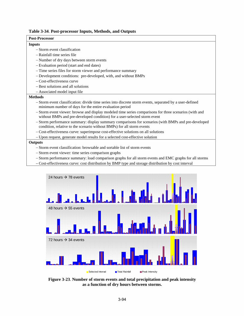
Table 3-34. Post-processor Inputs, Methods, and Outputs Post-Processor Inputs

− Storm event classification − Rainfall time series file − Number of dry days between storm events − Evaluation period (start and end dates) − Time series files for storm viewer and performance summary − Development conditions: pre-developed, with, and without BMPs − Cost-effectiveness curve − Best solutions and all solutions − Associated model input file

Methods − Storm event classification: divide time series into discrete storm events, separated by a user-defined

minimum number of days for the entire evaluation period − Storm event viewer: browse and display modeled time series comparisons for three scenarios (with and

without BMPs and pre-developed condition) for a user-selected storm event − Storm performance summary: display summary comparisons for scenarios (with BMPs and pre-developed

cond − Cost-effectiveness curve: sup ns − Upon request, generate model results for a selected cost-effective solution

ition, relative to the scenario without BMPs) for all storm events erimpose cost-effective solutions on all solutio

Outputs − Storm − Storm − Storm performance summary EMC graphs for all storms

event classification: browsable and sortable list of storm events event viewer: time series comparison graphs

: load comparison graphs for all storm events and − Cost-effectiveness curve: cost distribution by BMP type and storage distribution by cost interval

72 hours Æ 34 events

48 hours Æ 55 events

24 hours Æ 78 events

Selected Interval Total Rainfall Peak Intensity

Figure 3-23. Number of storm events and total precipitation and peak intensity as a function of dry hours between storms.

3-94

In the SUSTAIN post-processor, once the storm events are defined, the user has the option of sorting the events by total precipitation volume or by peak intensity, as shown in Figure 3-24. Note that the same event (August 9, 2001, 6:00 p.m.) has been highlighted in both Figure 3-23 and Figure 3-24. The event sorting provides additional insight into the details of the selected event relative to other events. For example, in terms of total rainfall volume, the selected event is in the 53rd percentile; however, in terms of peak intensity, it is in the 82nd percentile for the selected year. The derived storm event information is further explored by the storm event viewer and storm performance summary analysis as described in the next two sections.

53%

82%

Sorted by Total Precipitation Volume

Sorted by Peak Precipitation Intensity

Selected Interval (Percentile) Total Rainfall Peak Intensity

Figure 3-24. Precipitation events sorted by total precipitation volume and peak intensity.

3.6.2. Storm Event Viewer Once the storm events are defined, the user can select a specific storm event to visualize its detailed time series responses. The storm event viewer plots the time series data for comparison under the following three conditions: (1) existing development without BMPs, (2) existing development with BMPs, and (3 ) before development. The viewer illustrates how BMP performance changes with increasing or decreasing storm size. Four example storms are shown below for illustration the use of the viewer. Those storm events were derived using 24 dry hours as the storm separation criterion. Storm event 1 (Figure 3-25) is the selected interval highlighted previously in the storm classification figures.

In each of the storm viewer graphs, the blue shaded area represents the developed condition without BMPs (post-developed), the brown line represents the BMP scenario, and the green line represents t he pre-developed condition. Storm event 1 in Figure 3-25 shows excellent BMP performance because the outflow from the BMP scenario (brown line) is significantly reduced from the post-developed condition, indicating that the storm runoff was well controlled by the BMP installed. Figure 3-26 shows a slightly different response. Although the peak flow for this ev e nt is similar to that of the first one (slightly lower), the storm interval 2 generates significantly more outflow than storm event 1. This is because the pea k precipitation came after 2 hours of steady rainfall causing the ground to be saturated and thus more bypass flow through the BMPs. After the storm has ended, outflow persists for a number of hours because of the attenuation by BMPs in the drainage area.

3-95

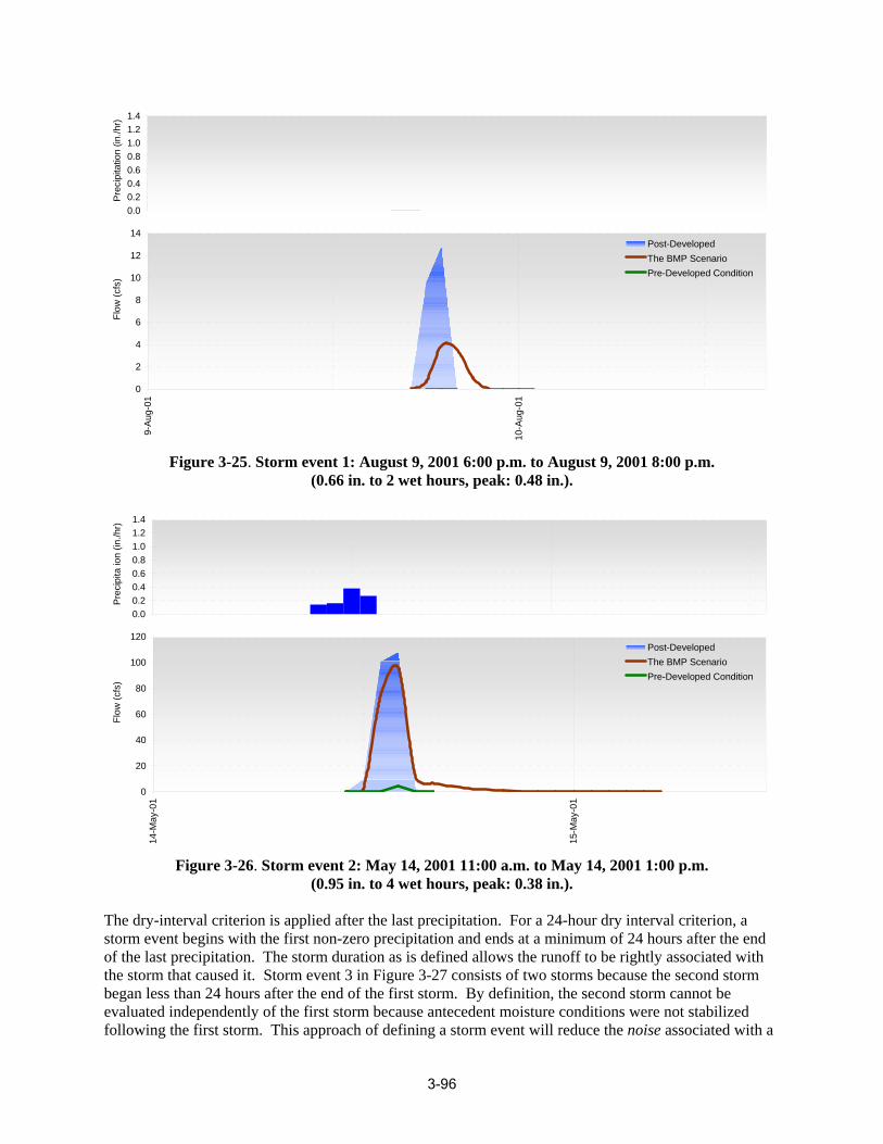
14

12

10

8

6

4

2

0

Post-Developed The BMP Scenario Pre-Developed Condition

9-A

ug-0

1

10-A

ug-0

1

Flow

(cfs

)

0.0 0.2 0.4 0.6 0.8 1.0 1.2 1.4

Pre

cipi

tatio

n (in

./hr)

Figure 3-25. Storm event 1: August 9, 2001 6:00 p.m. to August 9, 2001 8:00 p.m. (0.66 in. to 2 wet hours, peak: 0.48 in.).

3-96

14-M

ay-0

1

15-M

ay-0

1

0

20

40

60

80

100

120

Flow

(cfs

)

Post-Developed The BMP Scenario Pre-Developed Condition

0.0 0.2 0.4 0.6 0.8 1.0 1.2 1.4

Pre

cipi

taio

n (in

./hr)

Figure 3-26. Storm event 2: May 14, 2001 11:00 a.m. to May 14, 2001 1:00 p.m. (0.95 in. to 4 wet hours, peak: 0.38 in.).

The dry-interval criterion is applied after the last precipitation. For a 24-hour dry interval criterion, a storm event begins with the first non-zero precipitation and ends at a minimum of 24 hours after the e nd of the last precipitation. The storm duration as is defined allows the runoff to be rightly associated with the storm that caused it. Storm event 3 in Figure 3-27 consists of two storms because the second storm began less than 24 hours after the end of the first storm. By definition, the second storm cannot be evaluated independently of the first storm because antecedent moisture conditions were not stabilized following the first storm. This approach of defining a storm event will reduce the noise associated with a

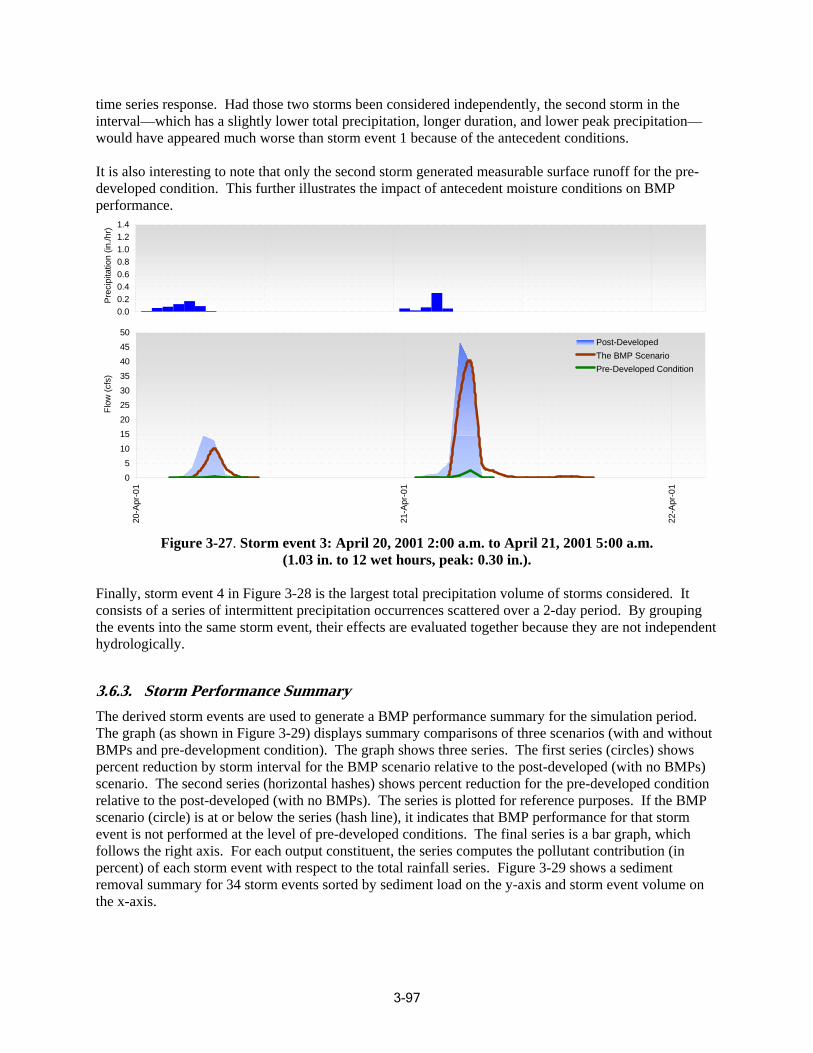
time series response. Had those two storms been considered independently, the second storm in the interval—which has a slightly lower total precipitation, longer duration, and lower peak precipitation— would have appeared much worse than storm event 1 because of the antecedent conditions.

It is also interesting to note that only the second storm generated measurable surface runoff for the pre-developed condition. This further illustrates the impact of antecedent moisture conditions on BMP performance.

0.0 0.2 0.4 0.6 0.8 1.0 1.2 1.4

Pre

cipi

tatio

n (in

./hr)

Flow

(cfs

)

50 45 40

35 30 25 20 15

10 5 0

Post-Developed Th e BMP Scenario Pre-Developed Condition

20-A

pr-0

1

21-A

pr-0

1

22-A

pr-0

1

Figure 3-27. Storm event 3: April 20, 2001 2:00 a.m. to April 21, 2001 5:00 a.m. (1.03 in. to 12 wet hours, peak: 0.30 in.).

Finally, storm event 4 in Figure 3-28 is the largest total precipitation volume of storms considered. It consists of a series of intermittent precipitation occurrences scattered over a 2-day period. By grouping the events into the same storm event, their effects are evaluated together because they are not independen t hydrologically.

3.6.3. Storm Performance Summary The derived storm events are used to generate a BMP performance summary for the simulation period. The graph (as shown in Figure 3-29) displays summary comparisons of three scenarios (with and without BMPs and pre-development condition). The graph shows three series. The first series (circles) shows percent reduction by storm interval for the BMP scenario relative to the post-developed (with no BMPs) scenario. The second series (horizontal hashes) shows percent reduction for the pre-developed condition relative to the post-developed (with no BMPs). The series is plotted for reference purposes. If the BMP scenario (circle) is at or below the series (hash line), it indicates that BMP performance for that storm event is not performed at the level of pre-developed conditions. The final series is a bar graph, which follows the right axis. For each output constituent, the series computes the pollutant contribution (in percent) of each storm event with respect to the total rainfall series. Figure 3-29 shows a sediment removal summary for 34 storm events sorted by sediment load on the y-axis and storm event volume on the x-axis.

3-97

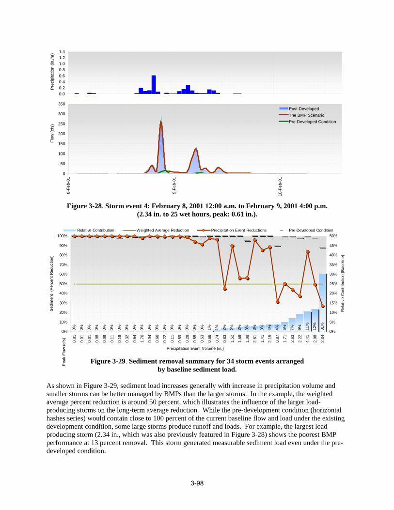
3-98

8-Fe

b-01

9-Fe

b-01

10-F

eb-0

1

0.0 0.2 0.4 0.6 0.8 1.0

Pre

cipi

tatio

n (in

1.2 1.4

./hr)

0

50

100

150

200

250

300

350

Flow

(cfs

)

Post-Developed The BMP Scenario Pre-Developed Condition

Figure 3-28. Storm event 4: February 8, 2001 12:00 a.m. to February 9, 2001 4:00 p.m . (2.34 in. to 25 wet hours, peak: 0.61 in.).

Precipitation Event Volume (in.)

10%

0% 0%

5%

Relative Contribution Weighted Average Reduction Precipitation Event Reductions Pre-Developed Condition

Sed

imen

t (P

erc e

nt R

educ

tion)

0.01

0.01

0.01

0.08

0.09

0.11

0.18

0.32

0.54

1.76

0.04

0.66

0.22

0.11

0.59

0.28

0.55

0.53

0.66

0.74

0.83

1.52

1.59

1.08

2.51

1.41

2.15

0.87

1.71

2.63

2.22

4.41

2.98

2.34

100%

0% 0% 0% 0% 0% 0% 0% 0% 0% 0% 0% 0% 0% 0% 0% 0% 0% 0% 1% 1% 2% 2% 2% 3% 3% 3% 4% 4% 5% 7% 9% 11%

12%

31%

50%

90% 45%

80% 40%

70% 35%

60% 30%

50% 25%

40% 20%

30% 15%

20% 10% Rel

ativ

e C

ontri

butio

n (B

asel

ine)

Pea

k Fl

ow (c

fs)

Figure 3-29. Sediment removal summary for 34 storm events arranged by baseline sediment load.

As shown in Figure 3-29, sediment load increases generally with increase in precipitation volume and smaller storms can be better managed by BMPs than the larger storms. In the example, the weigh ted average percent reduction is around 50 percent, which ill ustrates the influence of the larger load-producing storms on the long-term average reduction. While the pre-development condition (horizontal hashes series) would contain close to 100 percent of the current baseline flow and load under the existing development condition, some large storms produce runoff and loads. For example, the largest load producing storm (2.34 in., which was also previously featured in Figure 3-28) shows the poorest BMP performance at 13 percent removal. This storm generated measurable sediment load even under the pre-developed condition.

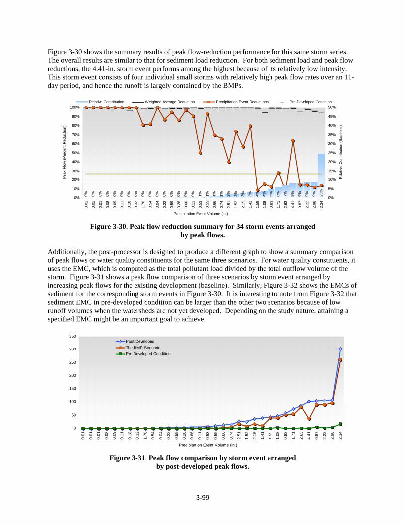
3-99

Figure 3-30 shows the summary results of peak flow-reduction performance for this same storm series. The overall results are similar to that for sediment load reduction. For both sediment load and peak flow reductions, the 4.41-in. storm event performs among the highest because of its relatively low intensity. This storm event consists of four individual small storms with relatively high peak flow rates over an 11­day period, and hence the runoff is largely contained by the BMPs.

Pea

k Fl

ow (P

erce

nt R

educ

tion)

Precipitation Event Volume (in.)

Relative Contribution Weighted Average Reduction Precipitation Event Reductions Pre-Developed Condition 100% 50%

90% 45%

0%

10%

0.01

0% 0% 0% 0% 0% 0% 0% 0% 0% 0% 0% 0% 0% 0% 0% 0% 1% 1% 1% 1% 2% 2% 3% 3% 4% 4% 5% 6% 7% 8% 9% 9% 9% 25%

0.01

0.01

0.08

0.09

0.11

0.18

0.32

1.76

0.54

0.04

0.22

0.59

0.28

80% 40%

70% 35%

60% 30%

50% 25%

40% 20%

30% 15%

20% 10% 0.

66

0.11

0.53

0.55

0.66

0.74

2.51

1.52

2.15

1.41

1.59

1.08

0.83

1.71

2.63

4.41

0.87

2.22

2.98

2.34

0%

5%

Rel

ativ

e C

ontri

butio

n (B

asel

ine)

Figure 3-30. Peak flow reduction summary for 34 storm events arranged by peak flows.

Additionally, the post-processor is designed to produce a different graph to show a summary comparison of peak flows or water quality constituents for the same three scenarios. For water quality constituents, it uses the EMC, which is computed as the total pollutant load divided by the total outflow volume of the storm. Figure 3-31 shows a peak flow comparison of three scenarios by storm event arranged by increasing peak flows for the existing development (baseline). Similarly, Figure 3-32 shows the EMCs of sediment for the corresponding storm events in Figure 3-30. It is interesting to note from Figure 3-32 that sediment EMC in pre-developed condition can be larger than the other two scenarios because of low runoff volumes when the watersheds are not yet developed. Depending on the study nature, attaining a specified EMC might be an important goal to achieve.

300

250

200

150

100

50

0

350 Post-Developed The BMP Scenario Pre-Developed Condition

Precipitation Event Volume (in.)

0.01

0.01

0.01

0.08

0.09

0.11

0.18

0.32

1.76

0.54

0.04

0.22

0.59

0.28

0.66

0.11

0.53

0.55

0.66

0.74

2.51

1.52

2.15

1.41

1.59

1.08

0.83

1.71

2.63

4.41

0.87

2.22

2.98

2.34

Figure 3-31. Peak flow comparison by storm event arranged by post-developed peak flows.

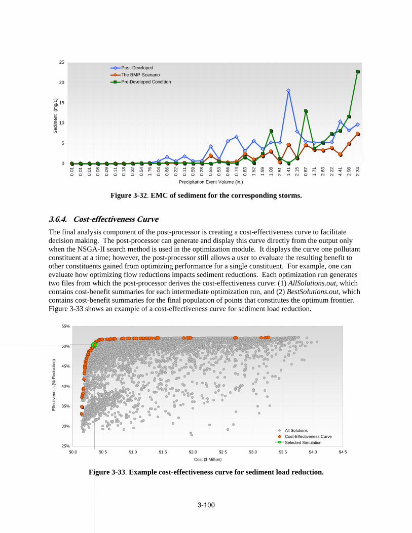
25

Post-Developed The BMP Scenario

20 Pre-Developed Condition

Sed

imen

t (m

g/L)

15

10

5

0

0.01

0.01

0.01

0.08

0.09

0.11

0.18

0.32

0.54

1.76

0.04

0.66

0.22

0.11

0.59

0.28

0.55

0.53

0.66

0.74

0.83

1.52

1.59

1.08

2.51

1.41

2.15

0.87

1.71

2.63

2.22

4.41

2.98

2.34

Precipitation Event Volume (in.) Figure 3-32. EMC of sediment for the corresponding storms.

3.6.4. Cost-effectiveness Curve The final analysis component of the post-processor is creating a cost-effectiveness curve to facilitate decision making. The post-processor can generate and display this curve directly from the output only when the NSGA-II search method is used in the optimization module. It displays the curve one pollutant constituent at a time; however, the post-processor still allows a user to evaluate the resulting benefit to other constituents gained from optimizing performance for a single constituent. For example, one can evaluate how optimizing flow reductions impacts sediment reductions. Each optimization run generates two files from which the post-processor derives the cost-effectiveness curve: (1) AllSolutions.out, which contains cost-benefit summaries for each intermediate optimization run, and (2) BestSolutions.out, which contains cost-benefit summaries for the final population of points that constitutes the optimum frontier. Figure 3-33 shows an example of a cost-effectiveness curve for sediment load reduction.

55%

50%

Effe

ctiv

enes

s (%

Red

uctio

n)

45%

40%

35%

25%

30%

$0.0 $0 5 $1.0 $1 5 $2.0 $2 5 $3.0 $3 5 $4.0

Cost ($ Million)

All Solutions Cost-Effectiveness Curve Selected Simulation

$4 5

Figure 3-33. Example cost-effectiveness curve for sediment load reduction.

3-100

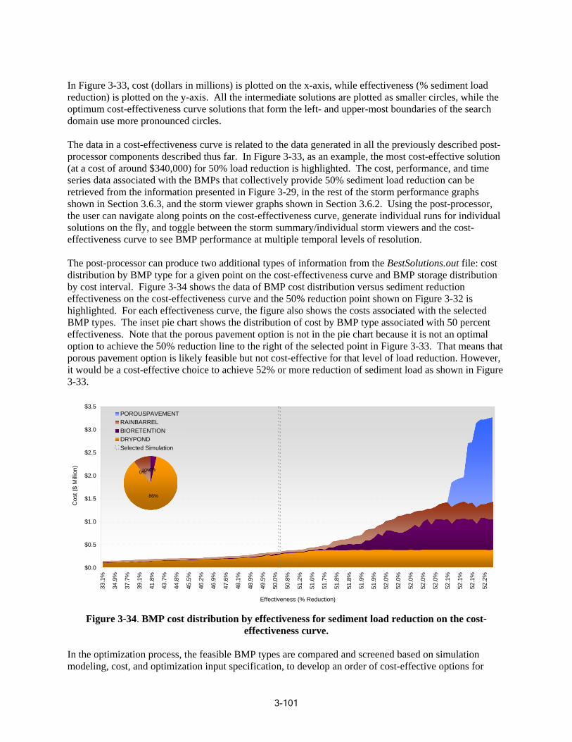
In Figure 3-33, cost (dollars in millions) is plotted on the x-axis, while effectiveness (% sediment load reduction) is plotted on the y-axis. All the intermediate solutions are plotted as smaller circles, while the optimum cost-effectiveness curve solutions that form the left- and upper-most boundaries of the search domain use more pronounced circle s.

The data in a cost-effectiveness curve is related to the data generated in all the previously described pos t-processor components described thus far. In Figure 3-33, as an example, the most cost-effective solution (at a cost of around $340,000) for 50% load reduction is highlighted. The cost, performance, and time series data associated with the BMPs that collectively provide 50% sediment load reduction can be retrieved from the information presented in Figure 3-29, in the rest of the storm performance graphs shown in Section 3.6.3, and the storm viewer graphs shown in Section 3.6.2. Using the post-processor, the user can navigate along points on the cost-effectiveness curve, generate individual runs for individual solutions on the fly, and toggle between the storm summary/individual storm viewers and the cost-effectiveness curve to see BMP performance at multiple temporal levels of resolution.

The post-processor can produce two additional types of information from the BestSolutions.out file: cost distribution by BMP type for a given point on the cost-effectiveness curve and BMP storage distribution by cost interval. Figure 3-34 shows the data of BMP cost distribution versus sediment reduction effectiveness on the cost-effectiveness curve and the 50% reduction point shown on Figure 3-32 is highlighted. For each effectiveness curve, the figure also shows the costs asso ciated with the selected BMP types. The inset pie chart shows the distribution of cost by BMP type associated with 50 percent effecti eness.v Note that the porous pavement option is not in the pie chart because it is not an optimal option to achieve the 50% reduction line to the right of the selected point in Figure 3-33. That means that porous pavement option is likely feasible b ut not cost-effective for that level of load reduction. However, it would be a cost-effective choice to achieve 52% or more reduction of sediment load as shown in Figure 3-33.

$0.0

$0.5

$1.0

$1.5

$2.0

$2.5

$3.0

$3.5

Cos

t ($

Milli

on)

POROUSPAVEMENT RAINBARREL BIORETENTION DRYPOND Selected Simulation

4%

86%

0%10%

33.1

%

34.9

%

37.7

%

39.1

%

41.8

%

43.7

%

44.8

%

45.5

%

46.2

%

46.9

%

47.6

%

48.1

%

48.9

%

49.5

%

50.0

%

50.8

%

51.2

%

51.6

%

51.7

%

51.8

%

51.8

%

51.9

%

51.9

%

52.0

%

52.0

%

52.0

%

52.0

%

52.0

%

52.1

%

52.1

%

52.1

%

52.2

%

Effectiveness (% Reduction)

Figure 3-34. BMP cost distribution by effectiveness for se diment load reduction on the cost-effectiveness curve.

In the optimization process, the feasible BMP types are compared and screened based on simulation modeling, cost, and optimization input specification, to develop an order of cost-effective options for

3-101

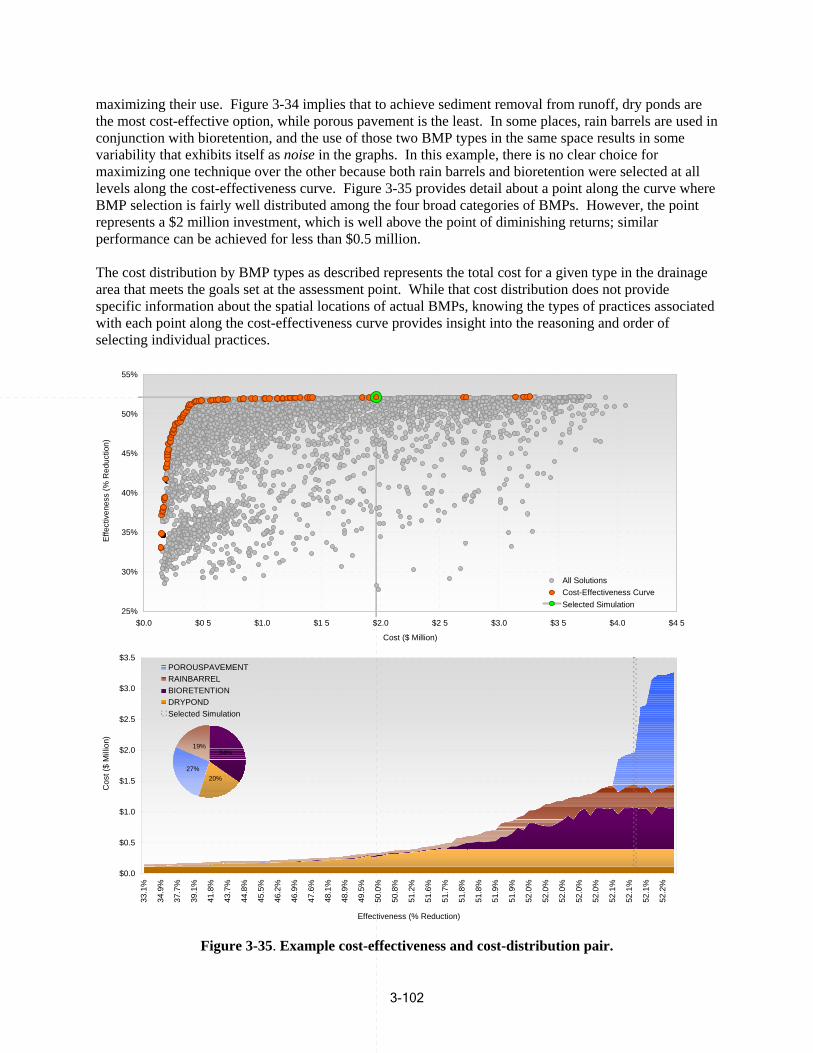
maximizing their use. Figure 3-34 implies that to achieve sediment removal from runoff, dry ponds are the most cost-effective option, while porous pavement is the least. In some places, rain barrels are used in conjunction with bioretention, and the use of those two BMP types in the same space results in some variability that exhibits itself as noise in the graphs. In this example, there is no clear choice for maximizing one technique over the other because both rain barrels and bioretention were selected at a ll levels along the cost-effectiveness curve. Figure 3-35 provides detail about a point along the curve where BMP selection is fairly well distributed among the four broad categories of BMPs. However, the point represents a $2 million investment, which is well above the point of diminishing returns; similar performance can be achieved for less than $0.5 million. The cost distribution by BMP types as described represents the total cost for a given type in the drainage area that meets the goals set at the assessment point. While that cost distribution does not provide specific information about the spatial locations of actual BMPs, knowing the types of practices associated with each point along the cost-effectiveness curve provides insight into the reasoning and order of selecting individual practices.

Cos

t ($

Mi lli

on)

Effe

ctiv

enes

s (%

Red

uctio

n)

55%

50%

45%

40%

35%

$3.5

$2.5

$3.0

25%

30%

$0.0

POROUSPAVEMENT RAINBARREL BIORETENTION DRYPOND Selected Simulation

$0 5 $1.0 $1 5 $2.0 $2 5

Cost ($ Million)

$3.0 $3 5 $4.0

All Solutions Cost-Effectiveness Curve Selected Simulation

$4 5

$1.5

$2.0 34%

20% 27%

19%

$1.0

$0.5

$0.0

33.1

%

34.9

%

37.7

%

39.1

%

41.8

%

43.7

%

44.8

%

45.5

%

46.2

%

46.9

%

47.6

%

48.1

%

48.9

%

49.5

%

50.0

%

50.8

%

51.2

%

51.6

%

51.7

%

51.8

%

51.8

%

51.9

%

51.9

%

52.0

%

52.0

%

52.0

%

52.0

%

52.0

%

52.1

%

52.1

%

52.1

%

52.2

%

Effectiveness (% Reduction)

Figure 3-35. Example cost-effectiveness and cost-distribution pair.

3-102

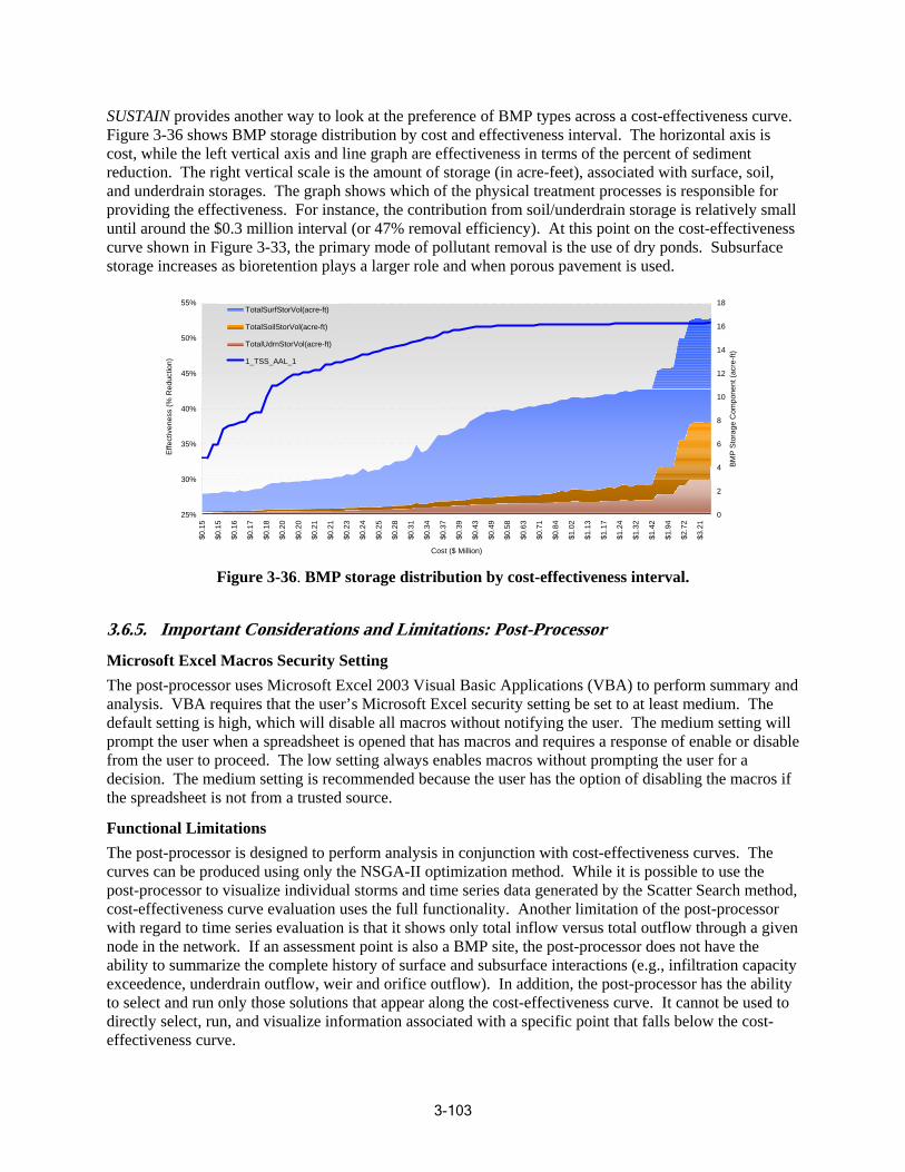
SUSTAIN provides another way to look at the preference of BMP types across a cost-effectiveness curve. Figure 3-36 shows BMP storage distribution by cost and effectiveness interval. The horizontal axis is cost, while the left vertical axis and line graph are effectiveness in terms of the percent of sediment reduction. The right vertical scale is the amount of storage (in acre-feet), associated with surface, soil, and underdrain storages. The graph shows which of the physical treatment processes is responsible for providing the effectiveness. For instance, the contribution from soil/underdrain storage is relatively small until around the $0.3 million interval (or 47% removal efficiency). At this point on the cost-effectiveness curve shown in Figure 3-33, the primary mode of pollutant removal is the use of dry ponds. Subsurface storage increases as bioretention plays a larger role and when porous pavement is used.

55% 18

Effe

ctiv

enes

s (%

Red

uctio

n)

50%

45%

40%

35%

30%

25%

TotalSurfStorVol(acre-ft)

TotalSoilStorVol(acre-ft)

TotalUdrnStorVol(acre-ft)

1_TSS_AAL_1

16

14

12

10

8

6

4

2

0

BMP

Sto

rage

Com

pone

nt (a

cre-

ft)

$0.1

5

$0.1

5

$0.1

6

$0.1

7

$0.1

8

$0.2

0

$0.2

0

$0.2

1

$0.2

1

$0.2

3

$0.2

4

$0.2

5

$0.2

8

$0.3

1

$0.3

4

$0.3

7

$0.3

9

$0.4

3

$0.4

9

$0.5

8

$0.6

3

$0.7

1

$0.8

4

$1.0

2

$1.1

3

$1.1

7

$1.2

4

$1.3

2

$1.4

2

$1.9

4

$2.7

2

$3.2

1

Cost ($ Million)

Figure 3-36. BMP storage distribution by cost-effectiveness interval.

3.6.5. Important Considerations and Limitations: Post-Processor Microsoft Excel Macros Security Setting The post-processor uses Microsoft Excel 2003 Visual Basic Applications (VBA) to perform summary and analysis. VBA requires that the user’s Microsoft Excel security setting be set to at least medi um. The default setting is high, which will disable all macros without notifying the user. The medium setting will prompt the user when a spreadsheet is op ened that has macros and requires a response of enable or disable from the user to proceed. The low se tting always enab les m acros without prompting the user for a decision. The medium setting is reco mmended because the user has the option of disabling the macros if the spreadsheet i s not from a trusted source.

Functional Limitations The post-processor is designed to perf orm analysis in conjunction with cost-effectiveness curves. The curves can be produced using only th e NSGA-II optim ization metho d. While it is possible to use the post-processor to visualize individual storms and time series data generated by the Scatter Search method, cost-effectiveness curve evaluation uses the full functi onality. Another limitatio n of the post-processor with regard to time series evaluation is that it shows o nly total inflow versus total outflow through a given node in the network. If an assessment point is also a BMP site, the post-processor does not have the ability to summarize th e complete history of surface a nd subsurface interactions (e.g., infiltration capacity exceedence, underdrain outflow, weir and orifice outflow ). In addition, the post-processor has the abilityto select and run only those solutions that appear along the cost-effectiveness curve. It cannot be used to directly select, run, and visualize information associat ed with a specific point that falls below the cost-effectiveness curve.

3-103

Chapter 4 Case Studies To best demonstrate the functionality and help users visualize how they can apply SUSTAIN, two case studies were developed for metropolitan areas that represent typical settings for applying the framewo rk. Case studies provide an excellent opportunity to explore the capabilities of SUSTAIN as described in this document in the context of a real life scenario and demonstrate the application process beginning with data collection, problem setup, optimization, and results interpretation. The examples were specifically developed to highlight the core functions of BMP placeme nt and selection and the associated development of the best solution for the user-defined problem. The case studies also demonstrate how to apply k e y functions such as the multi-scale, tiered analys is, and the use of multiple control targets for opti mi zation.

Ideal c se studies for testing a SUSTAIN should be consistent with the design requirements and the placem nt and selection of BMPs in urban are e as. For effective demonstration, the case studies also need to build on a history of monitoring data c ollection and analysis. The ideal case studies also have recent watershed-based studies that have resulted in calibrated and validated models that can be used for setup and comparison. The case studies were selected using the fo llowing criteria:

• Dominantly urban land use • Water quality management needs • History of data collection • Calibrated/validated model application

Two locations fit the criteria and were available for use—the Milwaukee Metropolitan Sewer District (MMSD) in Milwaukee, Wisconsin (the Oak Creek watershed), and Fairfax County, Virginia (the Little Rocky Run watershed). For each case study, locally derived data were used to develop the project setup and analysis. Next, specific problem objectives were identified that hig hlighted some important functions of SUSTAIN. For the Oak Creek watershed, the case study focuses on placement and selection of BMPs, using a single po llutant with a tiered approach, for effectiv eness evaluation at several targeted pollutant reduction goals. It also demonstrates how to integrate external model time series from an existing watershed model. For the Little Rocky Run watershed, the case study focused on placement and selection of BMPs on the basis of the evaluation of two concurrent control targets of peak flow and TSS reduction. It also demonstrates using the internal SWMM m odel for generating runoff and pollutant load time series. This chapter describes the pro ject setup, analysis process, and results interpretation for each case study.

Through the demonstrations, the flexibi lity and potential of the framework is shown. Future demonstratio ns and applicatio ns throughout the user community will provide valuable experiences and insights on both the full potential of the existing framework and recommendations for the continued improvement of SUSTAIN.

4.1. Upper North Branch Oak Creek Watershed Milwaukee is on the southwestern shore of Lake Michigan and is the largest city in Wisconsin and 2 3rd largest (by population) in the nation. Milwaukee is the main cultural and economic center of the se ven­county Greater Milwaukee A rea, with an estimated population of 2,014,032 as of 2008. Four major river

4-104

systems (Menomonee River, Kinnickinnic River, Oak Creek, and Root River) drain an area of more than 1,100 s q uare miles that ultimately discharges through the Milwaukee River, in downtow n Milwaukee, to the harbor and Lake Michigan. Upstream areas are predominantly rural and agricultural including dairy farm s and crops such as corn, soybeans, and alfalfa. Nearer to the metropolitan area are suburban areas and commuter communities. The downtow n region is densely urbanized and drained by a combined sewer system. Over the past 20 years the city and the Milwaukee Metropolitan Sewerage District (MMSD) have taken significant steps to address CSOs by constructing a major storage tunnel. The 7.1­m ile long Northwest S ide Relief Sewer is a deep tunnel that can hold up to 89 million gallons of wastewater. The region has also led the way with various green programs such as the Greenseams program and been an advocate of innovative stormwater management techniques such as rain gardens, rain barrels, and downspout disconnections. Major environmental issues in the region include increas ed loadings of sediment, nutrients, and pathogens associated with urbanization and agriculture, and in the urban center CSOs.

Regional water quality and environmental protection continue to be a priority in the area. Recognizing this need, the MMSD has led a long-range planning effort to identify improvements needed for its facilities to accommodate growth and protect water qu a lity through the year 2020. This effort is known as the MMSD 2020 Facility Plan. A related planning effort, known as the Regional Water Qual ity Management Plan Update (RWQMPU), was also conducted in coordination with the MMSD by the Southeastern Wisconsin Regional Planning Commission (SEWRPC) to update the regional water quality management plan for all the major watersheds draining through the greater Milwaukee area (SEWRPC 2007).

As part of the planning process, a comprehensive suite of models was applied to the four major tributarie s to assess current conditions and evaluate a range of management scenarios. Those models allowed planners to evaluate the potential water quality benefits of a range of implementation measures, includin g facility improvements and urban, suburban, and rural stormwater BMPs. The watershed modeling component was developed using LSPC (Tetra Tech and USEPA 2002). Hydrology and water quality models were developed and calibrated to provide a basis for modeling current conditions versus pot ential implementation scenarios. The modeling application was developed and tested using an extensive record of precipitation, flow, and water quality sampling. Calibration of the watershed models followed a sequential, hierarchical process that b egan with hydrology, followed by sediment erosion and transport, and, finally, calibration of chemical water quality.

The Kinnickinnic River, Menomonee River, Milwaukee River, and Oak Creek watershed models were linked to a model of the Lake Michigan estuary so that the impact of upstream water quantity and quality could be simulated. During the RWQMPU study, several year 2020-projected management scenarios to reduce nutrient, bacteria, and sediment loading were evaluated (SEWRPC 2007)

The history of environmental management, watershed planning, technical analyses, monitoring, and the availability of calibrated models made this location ideal for a case study application of SUSTAIN. A representative subwatershed, Oak Creek, was selected for examination for the case study, and TSS was selected as the pollutant for optimization and analysis. This case study examined the use of SUSTAIN for tiered analysis and BMP optimization for a single parameter.

4.1.1. Project Setting The Oak Creek watershed covers parts of the cities of Milwaukee, South Milwaukee, Cudahy, Franklin, Greenfield, and Oak Creek and encompasses approximately 27 square miles. Table 4-1 provides a listing of the main characteristics of the watershed.

4-105

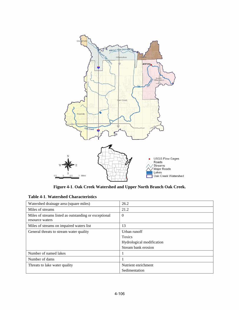
. Table 4-1 Watershed Characteristics

atershed drainage area (square miles) W 26.2 Miles of streams 21.2 Miles of streams listed as outstanding or exceptional resource waters

0

Miles of streams on impaired waters list 13 General threats to stream water quality Urban runoff

Toxics Hydrological modification Stream bank erosion

Number of named lakes 1 Number of dams 1

Threats to lake water quality Nutrient enrichment Sedimentation

Figure 4-1. Oak Creek Watershed and Upper North Branch Oak Creek.

4-106

The watershed has three major streams—Mitchell Field Drainage Ditch, North Branch of Oak Creek, and Oak Creek. The longest stream of the three, Oak Creek, has a perennial length of approximately 13.1 miles. North Branch of Oak Creek and Mitchell Field Drainage Ditch, which are tributaries to Oak Creek, have perennial lengths of approximately 5.8 and 2.4 miles, respectively. There is one reservoir in the watershed with a history of siltation and algal blooms.

Water quality in Oak Creek is degraded in part because of elevated sediment, sediment-associated total phosphorus, and fecal coliform loads. Because sediment data were closely correlated with nutrients specifically and peak discharges in general, TSS was selected as the pollutant on which to focus the case study analysis.

Pollution sources in the watershed include the following:

• Stormwater runoff from impervious urban land • Runoff from agricultural lands • Eroding streambanks and sedimentation • Wildlife, pets, and residential lawns • Erosion from construction sites • Sanitary sewer overflows and industrial discharges • Leaking undergroun d storage tanks, landf ills, runoff from salvage yards

The Upper North Branch O ak Creek (UNB ) area, shown in the upper-left corner of Figure 4-1, was selected for further evaluation in the case stud y. The UNB is a headwater area of concern because of poor habitat, elevated sediment load, a nd sediment-associated total phosphorus and fecal coliform loads. The UNB has a drainage area of approximately 4 .2 squ are miles with m ixed l and uses. The dominant residential and commercial land uses com pose 68 percent of the total area. Table 4-2 lists the land use distribution of the study area. The Oak Creek watershed has discharges from 17 industrial facilities as well as sa nitary sewer overflows.

Table 4-2. Uppe r North Bra nch Oak Creek Lan d Use Distributio n

Land U pese Ty ea

) Ar (acre

Area Percentage (%)

Water/wetland 41.0 2 Forest 7323. 12 Pasture/hay 88.5 3 Crop 4168. 6 Developed open space 263.4 10 C commer ial 342.0 13 High density residential 684.6 26 Low density residential 766.3 29 Total 2,677.7 100

The UNB watershed provides an excellent setting for demonstrating how SUSTAIN can be applied in the implementation and tracking aspects of a watershed planning process. For this application, a single objective of TSS load reduction was selected. In terms of SUSTAIN functionality, this case study demonstrates the following:

4-107

   

     

          

          

                

 

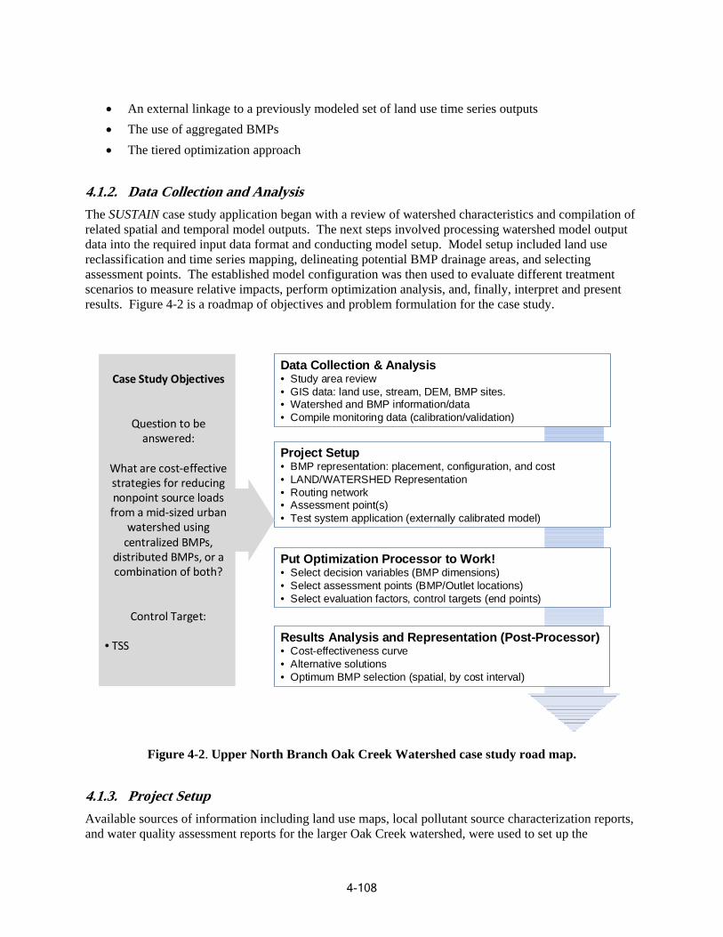
• An external linkage to a previously modeled set of land use time series outputs • The use of aggregated BMPs • The tiered optimization approach

4.1.2. Data Collection and Analysis The SUSTAIN case study application began with a review of watershed characteristics and compilation of related spatial and temporal model outputs. The next steps involved processing watershed model output data into the required input data format and conducting model setup. Model setup included land use reclassification and time series mapping, delineating potential BMP drainage areas, and selecting assessment points. The established model configuration was then used to evaluate different treatment scenarios to measure relative impacts, perform optimization analysis, and, finally, interpret and present results. Figure 4-2 is a roadmap of objectives and problem formulation for the case study.

Results Analysis and Representation (Post-Processor) • Cost-effectiveness curve • Alternative solutions • Optimum BMP selection (spatial, by cost interval)

Put Optimization Processor to Work! • Select decision variables (BMP dimensions) • Select assessment points (BMP/Outlet locations) • Select evaluation factors, control targets (end points)

Project Setup • BMP representation: placement, configuration, and cost • LAND/WATERSHED Representation • Routing network • Assessment point(s) • Test system application (externally calibrated model)

Data Collection & Analysis • Study area review • GIS data: land use, stream, DEM, BMP sites. • Watershed and BMP information/data • Compile monitoring data (calibration/validation)

Case Study Objectives

Question to be answered:

What are cost‐effective strategies for reducing nonpoint source loads from a mid‐sized urban

watershed using centralized BMPs,

distributed BMPs, or a combination of both?

Control Target:

• TSS

Figure 4-2. Upper North Branch Oak Creek Watershed case study road map.

4.1.3. Project Setup Available sources of information including land use maps, local pollutant source characterization reports, and water quality assessment reports for the larger Oak Creek watershed, were used to set up the

4-108

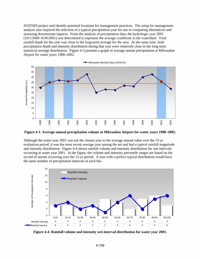
SUSTAIN project and identify potential locations for management practices. The setup for management analysis also required the selection of a typical precipitation year for use in comparing alternatives and assessing downstream impacts. From the analysis of precipitation data, the hydrologic year 2001 (10/1/2000–9/30/2001) was determined to represent the average conditions in the watershed. Total rainfall depth for the year was close to the long-term average for the area. At the same time, both precipitation depth and intensity distribution during that year were relatively close to the long-term statistical average distribution. Figure 4-3 presents a graph of average annual precipitation at Milwaukee Airport for water years 1988–2002.

4-109

0

5

10

15

20

25

30

35

40

45

50

)An

nual

Pre

cipi

tatio

n (in

.

Milwaukee Mitchell Airport (WI5479)

1988

1989

1990

1991

1992

1993

1994

1995

1996

1997

1998

1999

2000

2001

2002

Figure 4-3. Average annual precipitation volume at Milwaukee Airport for water years 1988–2002.

Although the water year 2001 was not the closest year to the average annual value over the 15-yr evaluation period, it was the most recent average year among the set and had a typical rainfall magnitude and intensity distribution. Figure 4-4 shows rainfall volume and intensity distribution for wet intervals occurring in water year 2001. In the figure, the volume and intensity percentile ranges are based on the record of storms occurring over the 15-yr period. A year with a perfect typical distribution would have the same number of precipitation intervals in each bin.

Num

ber o

f Pre

cipi

tatio

n In

terv

als

0

2

4

6

8

10

12

14 Rainfall Intensity

Rainfall Volume

Rainfall Intensity 3 3 2 3 5 4 2 5 6 3

Rainfall Volume 3 4 2 3 1 4 6 2 5 6

0-10 10-20 20-30 30-40 40-50 50-60 60-70 70-80 80-90 90-100

Figure 4-4. Rainfall volume and intensity wet-interval distribution for water year 2001.

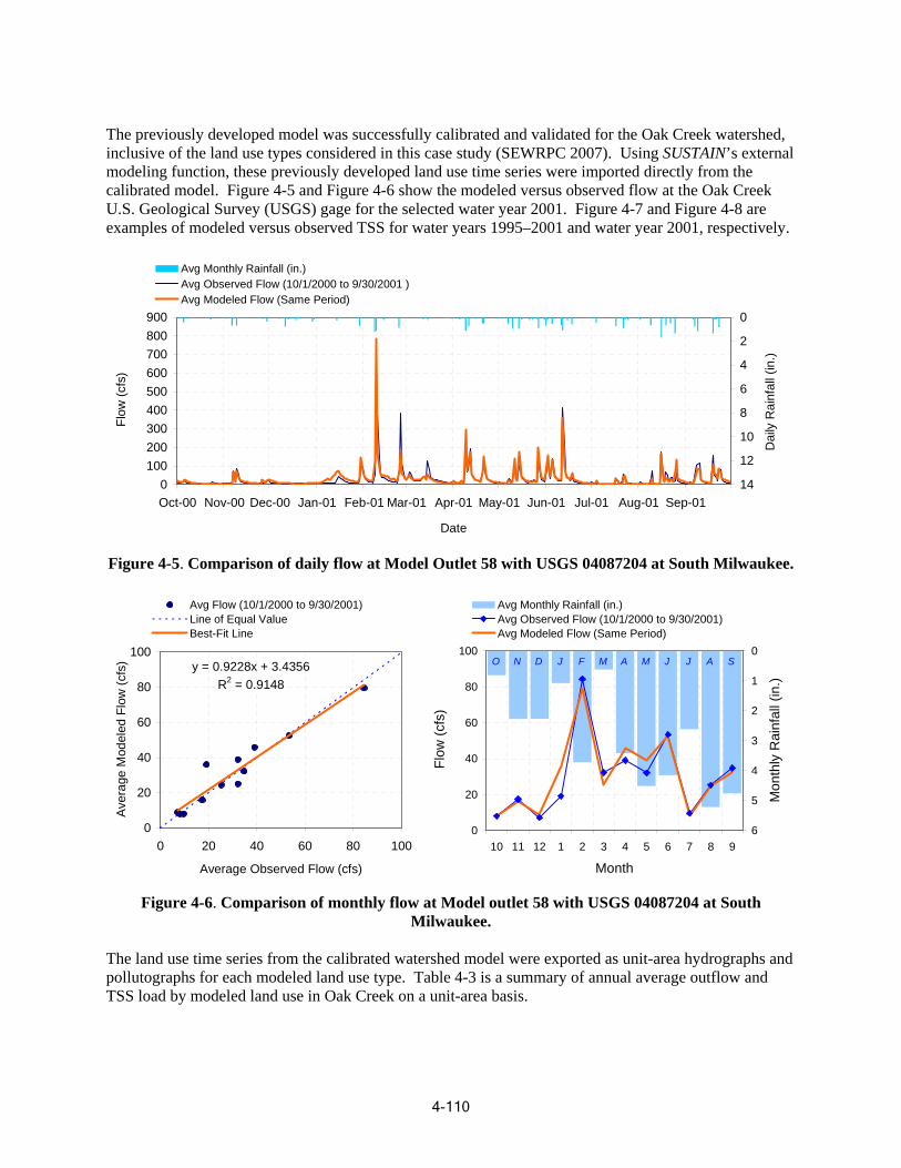
The previously developed model was successfully calibrated and validated for the Oak Creek watershed, inclusive of the land use types considered in this case study (SEWRPC 2007). Using SUSTAIN’s external modeling function, these previously developed land use time series were imported directly from the calibrated model. Figure 4-5 and Figure 4-6 show the modeled versus observed flow at the Oak Creek U.S. Geological Survey (USGS) gage for the selected water year 2001. Figure 4-7 and Figure 4-8 are examples of modeled versus observed TSS for water years 1995–2001 and water year 2001, respectively.

Avg Monthly Rainfall (in.) Avg Observed Flow (10/1/2000 to 9/30/2001 ) Avg Modeled Flow (Same Period)

0 100 200 300 400 500 600 700 800 900

Flow

(cfs

)

0

2

4

6

8

10

12

14

Dai

ly R

ainf

all (

in.)

Oct-00 Nov-00 Dec-00 Jan-01 Feb-01 Mar-01 Apr-01 May-01 Jun-01 Jul-01 Aug-01 Sep-01

Date

Figure 4-5. Comparison of daily flow at Model Outlet 58 with USGS 04087204 at South Milwaukee.

Avg Flow (10/1/2000 to 9/30/2001) Avg Monthly Rainfall (in.) Line of Equal Value Avg Observed Flow (10/1/2000 to 9/30/2001) Best-Fit Line Avg Modeled Flow (Same Period)

100 100 O N D J F M A M J J A S

0

1

2

3

4

5 Mon

thly

Rai

nfal

l (in

.)

Ave

rage

Mod

eled

Flo

w (c

fs) y = 0.9228x + 3.4356

R2 = 0.9148 80

60

40

80

Flow

(cfs

)

60

40

20 20

0 0 6

0 20 40 60 80 100 10 11 12 1 2 3 4 5 6 7 8 9

Average Observed Flow (cfs) Month

Figure 4-6. Comparison of monthly flow at Model outlet 58 with USGS 04087204 at South Milwaukee.

The land use time series from the calibrated watershed model were exported as unit-area hydrographs and pollutographs for each modeled land use type. Table 4-3 is a summary of annual average outflow and TSS load by modeled land use in Oak Creek on a unit-are a basis.

4-110

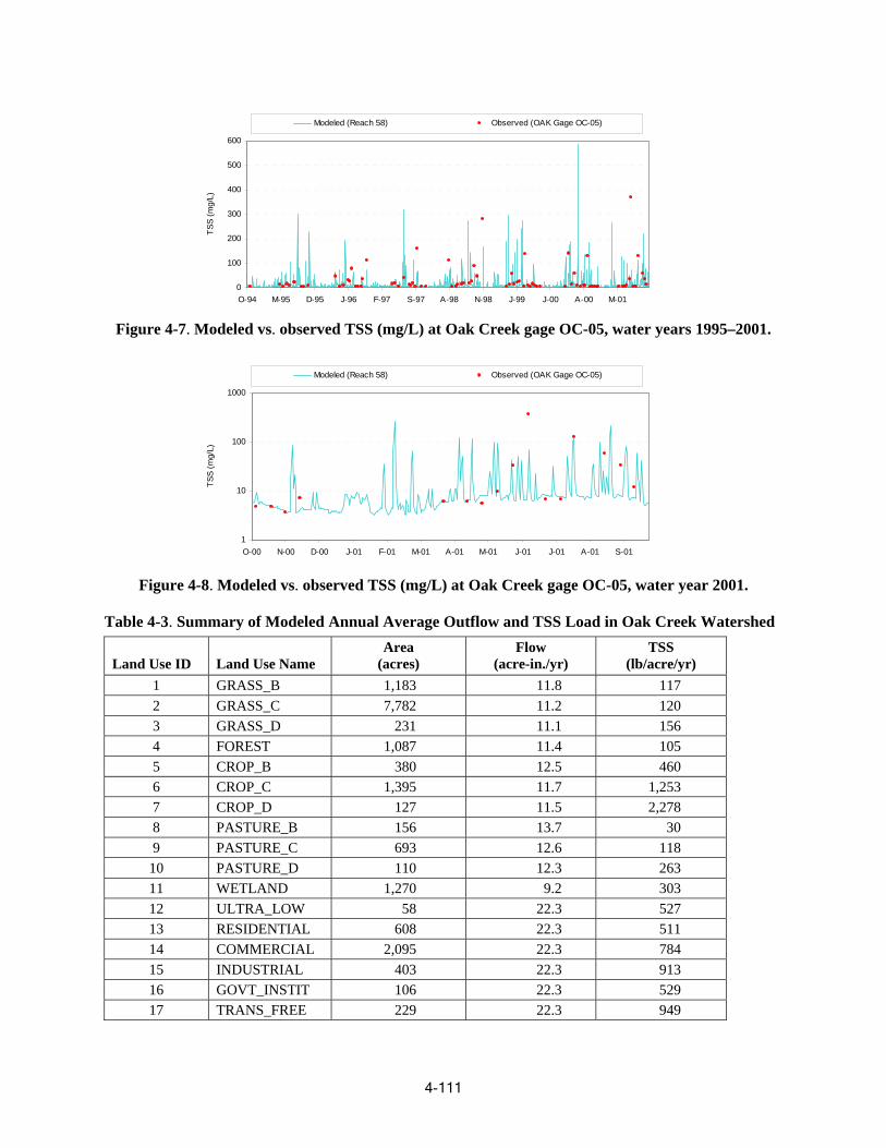
Modeled (Reach 58) Obser ved (OAK Gage OC-05)

0

100

200

T 300

400

0

600

SS (m

g/L)

50

O-94 M-95 D-95 J-96 F-97 S-97 A-98 N-98 J-9 9 J-00 A-00 M-01

Figure 4-7. Modeled vs. observed TSS (mg/L) at Oak Creek gage OC-05, water years 1995–2001.

Modeled (Reach 58) Observed (OAK Gage OC-05)

1000

) 100

L /g (mS

TS

10

1

O-00 N-00 D-00 J-01 F-01 M-01 A-01 M-01 J-01 J-01 A-01 S-01

Figure 4-8. Modeled vs. observed TSS (mg/L) at Oak Creek gage OC-05, water year 2001.

Table 4-3. Summary of Modeled Annual Average Outflow and TSS Load in Oak Creek Watershed

Land Use ID Land Use Name Area

(acres) Flow

(acre-in./yr) TSS

(lb/acre/yr) 1 GRAS S_B 1,183 11.8 117 2 GRASS_C 7,782 11.2 120 3 GRASS_D 231 11.1 156 4 FOREST 1,087 11.4 105 5 CROP_B 380 12.5 046 6 CROP_C 1,395 11.7 1,253 7 CROP_D 127 11.5 2,278 8 PASTURE_B 156 13.7 30 9 PASTURE_C 693 12.6 118

10 PASTURE_D 110 12.3 263 11 WETLAND 1,270 9.2 303 12 ULTRA_LOW 58 22.3 527 13 RESIDENTIAL 608 22.3 511 14 COMMERCIAL 2,095 22.3 784 15 INDUSTRIAL 403 22.3 913 16 GOVT_INSTIT 106 22.3 529 17 TRANS_FREE 229 22.3 949

4-111

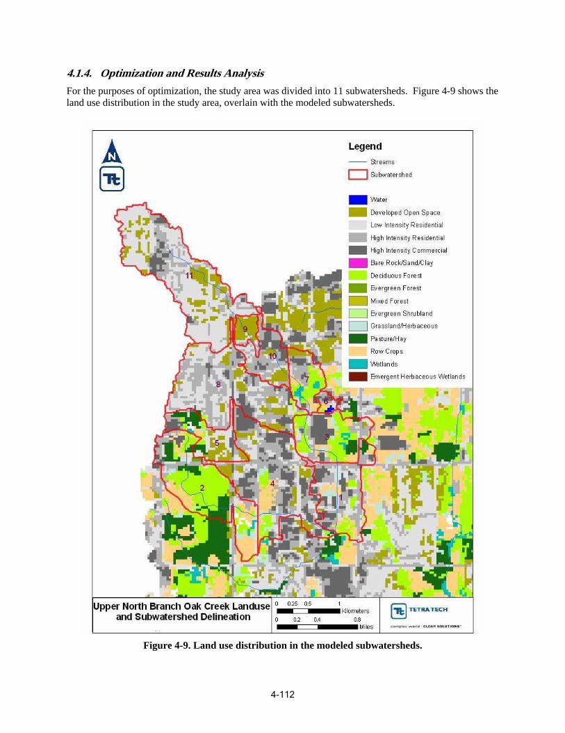
4.1.4. Optimization and Results Analysis For the purposes of optimization, the study area was divided into 11 subwatersheds. Figure 4-9 shows the land use distribution in the study area, overlain with the modeled subwatersheds.

Figure 4-9. Land use distribution in the modeled subwatersheds.

4-112

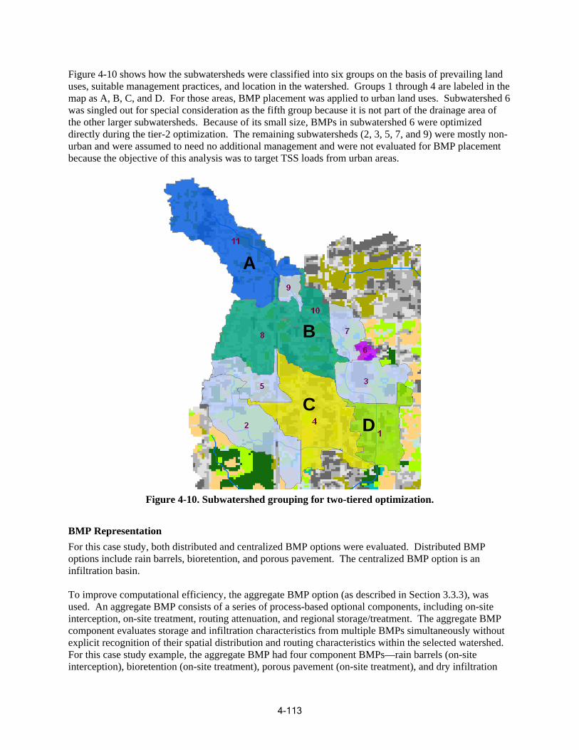
Figure 4-10 shows how the s ubwatersheds were classified into six groups on the basis of prevailing land uses, suitable management practices, and location in the watershed. Groups 1 through 4 are labeled in the map as A, B, C, and D. For those areas, BMP placement was applied to urban land uses. Subwatershed 6 was singled out for special consideration as the fifth group because it is not part of the drainage area of the other larger subwatersheds. Because of its small size, BMPs in subwatershed 6 were optimized directly during the tier-2 optimization. The remaining subwatersheds (2, 3, 5, 7, and 9) were mostly non-urban and were assumed to need no additional management and were not evaluated for BMP placement because the objective of this analysis was to target TSS loads from urban areas.

A

B

C D

Figure 4-10. Subwatershed grouping for two-tiered optimization.

BMP Representation For this case study, both distributed and centralized BMP options were evaluated. Distributed BMP options include rain barrels, bioretention, and porous pavement. The centralized BMP option is an infiltration basin.

To improve computational efficiency, the aggregate BMP option (as described in Section 3.3.3), was used. An aggregate BMP consists of a series of process-based optional components, including on-site interception, on-site treatment, routing attenuation, and regional storage/treatment. The aggregate BMP component evaluates storage and infiltration characteristics from multiple BMPs simultaneously without explicit recognition of their spatial distribution and routing characteristics within the selected watershed. For this case study example, the aggregate BMP had four component BMPs—rain barrels (on-site interception), bioretention (on-site treatment), porous pavement (on-site treatment), and dry infiltration

4-113

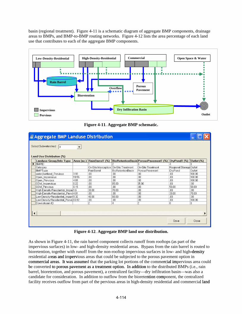
basin (regional treatment). Figure 4-11 is a schematic diagram of aggregate BMP components, drainage areas to BMPs, and BMP-to-BMP routing networks. Figure 4-12 lists the area percentage of each land use that contributes to each of the aggregate BMP components.

Outlet

Commercial

Overflow

Low-Density-Residential

Rain Barrel

Dry Infiltration Basin

Bioretention

Porous Pavement

High-Density-Residential Open Space & Water

Impervious Pervious

Figure 4-11. Aggregate BMP schematic.

Figure 4-12. Aggregate BMP land use distribution.

As shown in Figure 4-11, the rain barrel component collects runoff from rooftops (as part of theimpervious surfaces) in low- and high-density residential areas. Bypass from the rain barrel is routed tobioretention, together with runoff from the non-rooftop impervious surfaces in low- and high--dd ensityensityresidential areas and ieas and imperpervvious areas that could be subjected to the porous pavement option incocommercial ammercial areas.reas. It waIt was as assussummeed that the parking lot portions of the commercirciaa l il immpervious area couldbbe converted to porto porous pavous paveemmeent as nt as a treatma treatment optionent option.. In additiIn additionon to the distributed BMPs (i.e., rainbarrel, bioretention, and porous pavement), a centralized facility—dry infiltration basin—was also acandidate for consideration. In addition to outflow from the bioretenntion comtion component, the centralizedfacility receives outflow from part of the pervious areas in high-density residential and commercial landl land

4-114

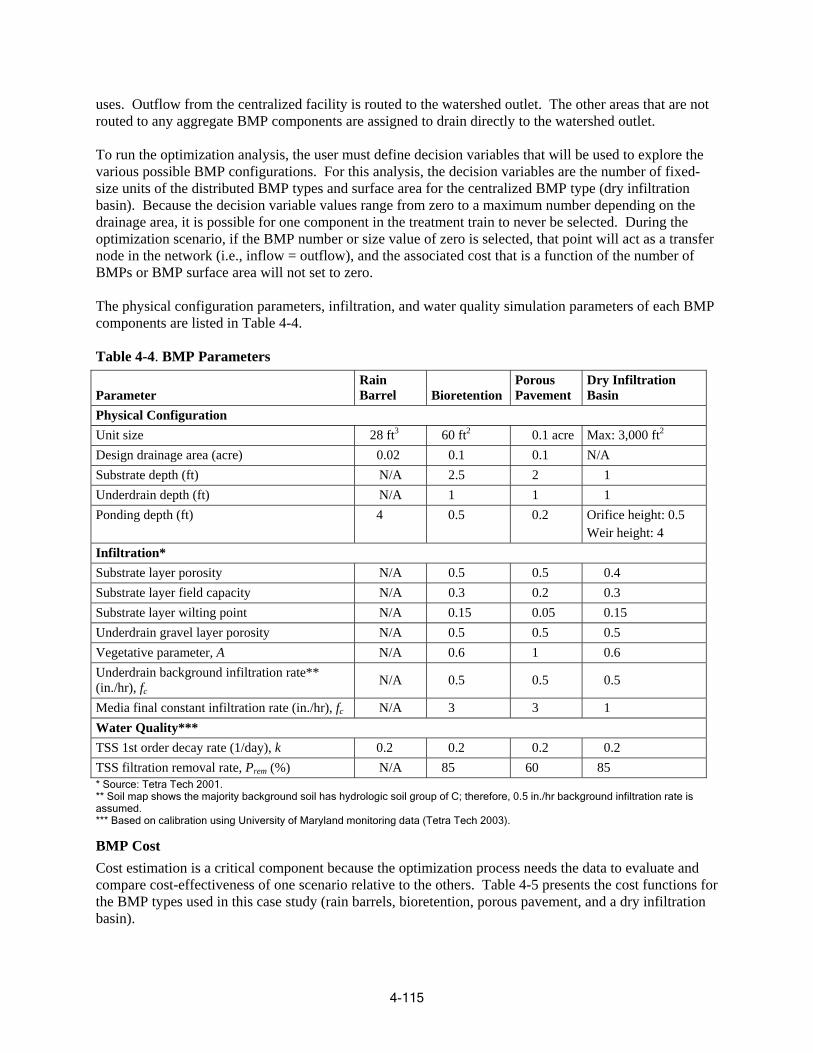
uses. Outflow from the centralized facility is routed to the watershed outlet. The other areas that are n ot routed to any aggregate BMP components are assigned to drain directly to the watershed outlet.

To run the optimization analysis, the user must define decision variables that will be used to explore th e various possible BMP configurations. For this analysis, the decision variables are the number of fixed-size units of the distributed BMP types and surface area for the centralized BMP type (dry infiltrat ion basin). Because the decision variable values range from zero to a maximum number depending o n the drainage area, it is possible for one component in the treatment train to never be selected. During the optimization scenario, if the BMP number or size value of zero is selected, that point w ill act as a transfer node in the network (i.e., inflow = outflow), and the associated cost that is a function of the number of BMPs or BMP surface area will not set to zero.

The physical configuration parameters, infiltration, and water quality simulation parameters of each BMP components are listed in Table 4-4.

Table 4-4. BMP Parameters

Parameter Rain Barrel Bioretention

Porous Pavement

Dry Infiltration Basin

Physical Configuration Unit size 28 ft3 60 ft2 0.1 acre Max: 3,000 ft2

Design drainage area (acre) 0.02 0.1 0.1 N/A Substrate depth (ft) N/A 2.5 2 1 Underdrain depth (ft) N/A 1 1 1 Ponding depth (ft) 4 0.5 0.2 Orifice height: 0.5

Weir height: 4 Infiltration* Substrate layer porosity N/A 0.5 0.5 0.4 Substrate layer field capacity N/A 0.3 0.2 0.3 Substrate layer wilting point N/A 0.15 0.05 0.15 Underdrain gravel layer porosity N/A 0.5 0.5 0.5 Vegetative parameter, A N/A 0.6 1 0.6 Underdrain background infiltration rate** (in./hr), fc

N/A 0.5 0.5 0.5

Media final constant infiltration rate (in./hr), fc N/A 3 3 1 Water Quality*** TSS 1st order decay rate (1/day), k 0.2 0.2 0.2 0.2 TSS filtration removal rate, Prem (%) N/A 85 60 85 * Source: Tetra Tech 2001. ** Soil map shows the majority background soil has hydrologic soil group of C; therefore, 0.5 in./hr background infiltration rate is assumed. *** Based on calibration using University of Maryland monitoring data (Tetra Tech 2003).

BMP Cost Cost estimation is a critical component because the optimization process needs the data to evaluate and compare cost-effectiveness of one scenario relative to the others. Table 4-5 presents the cost functions for the BMP types used in this case study (rain barrels, bioretention, porous pavement, and a dry infiltra tion basin).

4-115

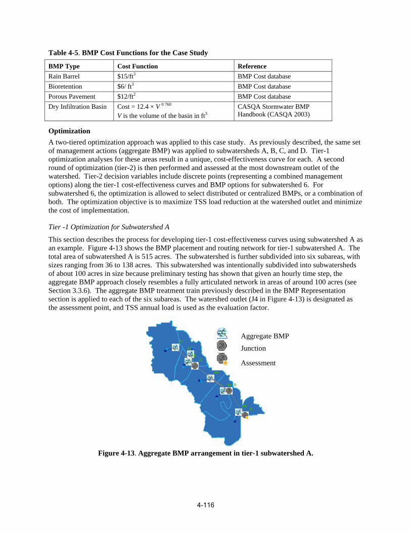
Table 4-5. BMP Cost Functions for the Case Study

BMP Type Cost Function Reference Rain Barrel $15/ft3 BMP Cost database Bioretention $6/ ft3 BMP Cost database Porous Pavement $12/ft2 BMP Cost database Dry Infiltration Basin Cost = 12.4 × V 0 760

V is the volume of the basin in ft3 CASQA Stormwater BMP Handbook (CASQA 2003)

Optimization A two-tiered optimization approach was applied to this case study. As previously described, the same set of management actions (aggregate BMP) was applied to subwatersheds A, B, C, and D. Tier-1 optimization analyses for these areas result in a unique, cost-effectiveness curve for each. A second round of optimization (tier-2) is then performed and assessed at the most downst ream outlet of the waters h ed. Tier-2 decision variables include discrete points (representing a com bined management option s ) along the tier-1 cost-effectiveness curves and BMP options for subwat ershed 6. For subwatershed 6, the optimization is allowed to select distributed or centralized BMPs, or a comb ination of both. The optimization objective is to maximize TSS load reduction at the watershed outlet and minimize the cost of implementation.

Tier -1 Optimization for Subwatershed A

This section describes the process for developing tier-1 cost-effectiveness curves using subwatershed A as an example. Figure 4-13 shows the BMP placement and routing network for tier-1 subwatershed A. The total area of subwatershed A is 515 acres. The subwatershed is further subdivided into six subareas, with sizes ranging from 36 to 138 acres. This subwatershed was intentionally subdivided into subwatersheds of about 100 acres in size because preliminary testing has shown that given an hourly time step, the aggregate BMP approach closely resembles a fully articulated network in areas of around 100 acres (see Section 3.3.6). The aggregate BMP treatment train previously described in the BMP Representation section is applied to each of the six subareas. The watershed outlet (J4 in Figure 4-13) is designated as the assessment point, and TSS annual load is used as the evaluation factor.

Figure 4-13. Aggregate BMP arrang

4-116

Aggregate BMP

Junction

Assessment

ement in tier-1 subwatershed A.

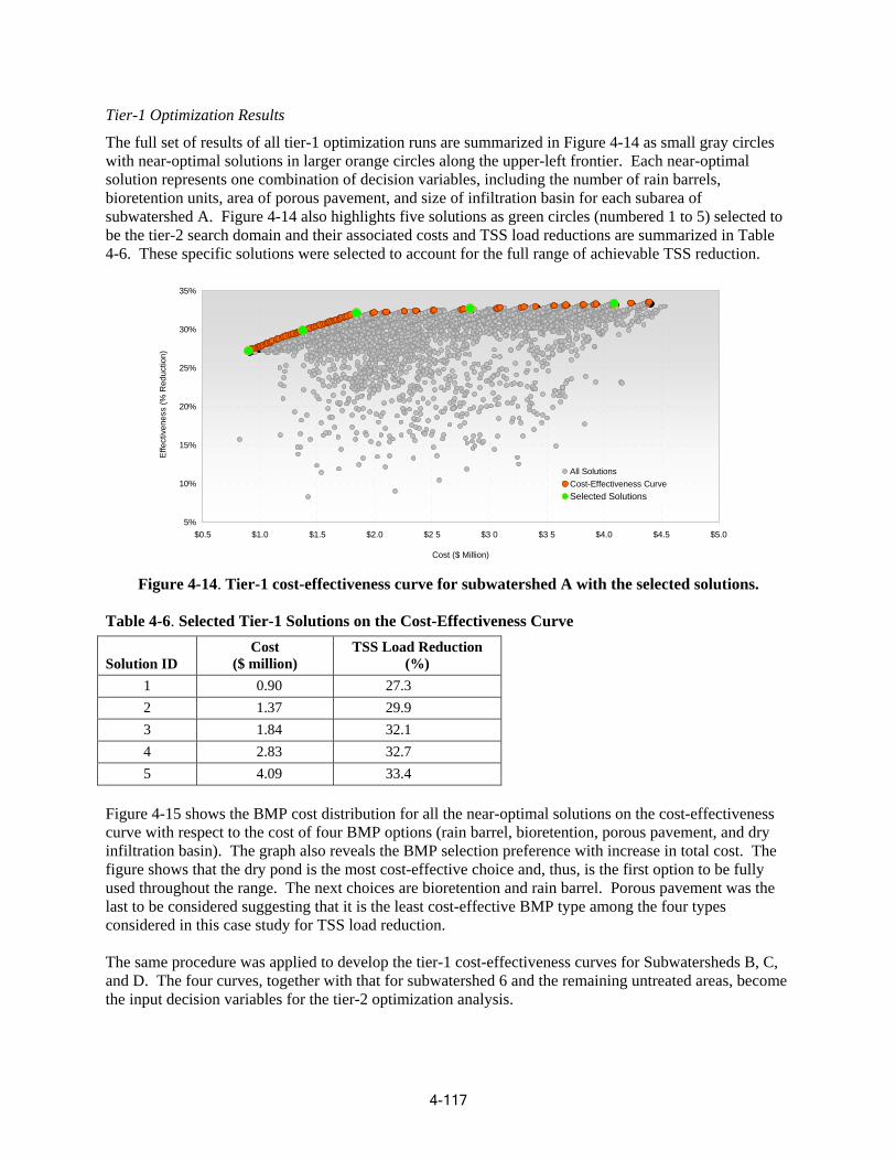
Tier-1 Optimization Results

The full set of results of all tier-1 optimization runs are summarized in Figure 4-14 as small gray circles with near-optimal solutions in larger orange circles along the upper-left frontier. Each near-optimal solution represents one combination of decision variables, including the number of rain barrels, bioretention units, area of porous pavement, and size of infiltration basin for each subarea of subwatershed A. Figure 4-14 also highlights five solutions as green circles (numbered 1 to 5) selected to be the tier-2 search domain and their associated costs and TSS load reductions are summarized in Table 4-6. These specific solutions were selected to account for the full range of achievable TSS reduction.

Effe

ctiv

enes

s (%

Red

uctio

n)

35%

30%

25%

20%

15%

All Solutions

10% Cost-Effectiveness Curve Selected Solutions

5% $0.5 $1.0 $1.5 $2.0 $2 5 $3 0 $3 5 $4.0 $4.5 $5.0

Cost ($ Million)

Figure 4-14. Tier-1 cost-effectiveness curve for subwatershed A with the selected solutions.

Table 4-6. Selected Tier-1 Solutions on the Cost-Effectiveness Curve Cost TSS Load Reduction

Solution ID ($ million) (%) 1 0.90 27.3 2 1.37 29.9 3 1.84 32.1 4 2.83 32.7 5 4.09 33.4

Figure 4-15 shows the BMP cost distribution for all the near-optimal solutions on the cost-effectiveness curve with respect to the cost of four BMP options (rain barrel, bioretention, porous pavement, and dry infiltration basin). The graph also reveals the BMP selection preference with increase in total cost. The figure shows that the dry pond is the most cost-effective choice and, thus, is the first option to be fully used throughout the range. The next choices are bioretention and rain barrel. Porous pavement was the last to be considered suggesting that it is the least cost-effective BMP type among the four types considered in this case study for TSS load reduction. The same procedure was applied to develop the tier-1 cost-effectiveness curves for Subwatersheds B, C, and D. The four curves, together with that for subwatershed 6 and the remaining untreated areas, become the input decision variables for the tier-2 optimization analysis.

4-117

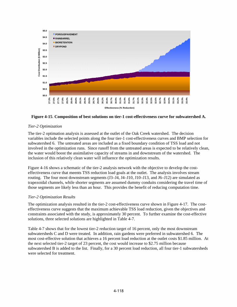
Cos

t Dis

tribu

tion

($ M

illio

n)

$5.0

$4.5

$4.0

$3.5

$3.0

$2.5

$2.0

$1.5

$1.0

$0.5

$0.0

POROUSPAVEMENT

RAINBARREL BIORETENTION

DRYPOND 27

.3%

27.5

%

27.7

%

27.9

%

28.2

%

28.4

%

28.8

%

29.1

%

29.4

%

29.5

%

29.7

%

29.9

%

30.2

%

30.4

%

30.7

%

30.9

%

31.1

%

31.4

%

31.6

%

31.7

%

32.1

%

32.3

%

32.4

%

32.5

%

32.6

%

32.7

%

32.9

%

33.0

%

33.1

%

33.2

%

33.3

%

33.4

%

Effectiveness (% Reduction)

Figure 4-15. Composition of best solutions on tier-1 cost-effectiveness curve for subwatershed A.

Tier-2 Optimization

The tier-2 optimation analysis is assessed at the outlet of the Oak Creek watershed. The decision variables include the selected points along the four tier-1 cost-effectiveness curves and BMP selection for subwatershed 6. The untreated areas are included as a fixed boundary condition of TSS load and not involved in the optimization runs. Since runoff from the untreated areas is expected to be relatively clean, the water would boost the assimilative capacity of streams in and downstream of the watershed. The inclusion of this relatively clean water will influence the optimization results.

Figure 4-16 shows a schemati c of the tier-2 analysis network with the objective to develop the cost-effectiveness curve that meents TSS reduction load goals at the outlet. The analysis involves stream routing. The four most downstream segments (J3–J4, J4–J10, J10–J13, and J6–J12) are simulated as trapezoidal channels, while shorter segments are assumed dummy conduits considering the travel time of those segments are likely less than an hour. This provides the benefit of reducing computation time.

Tier-2 Optimization Results

The optimization analysis resulted in the tier-2 cost-effectiveness curve shown in Figure 4-17. The cost-effectiveness curve suggests that the maximum achievable TSS load reduction, given the objec tives and constraints associated with the study, is approximately 30 percent. To further examine the cost-effective solutions, three selected solutions are highlighted in Table 4-7.

Table 4-7 shows that for the lowest tier-2 reduction target of 16 percent, only the most downstream subwatersheds C and D were treated. In addition, rain gardens were preferred in subwatershed 6. The most cost-effective solution that achieves a 16 percent load reduction at the outlet costs $1.85 million. At the next selected tier-2 target of 23 percent, the cost would increase to $2.75 million because subwatershed B is added to the list. Finally, for a 30 percent load reduction, all four tier-1 subwatersheds were selected for treatment.

4-118

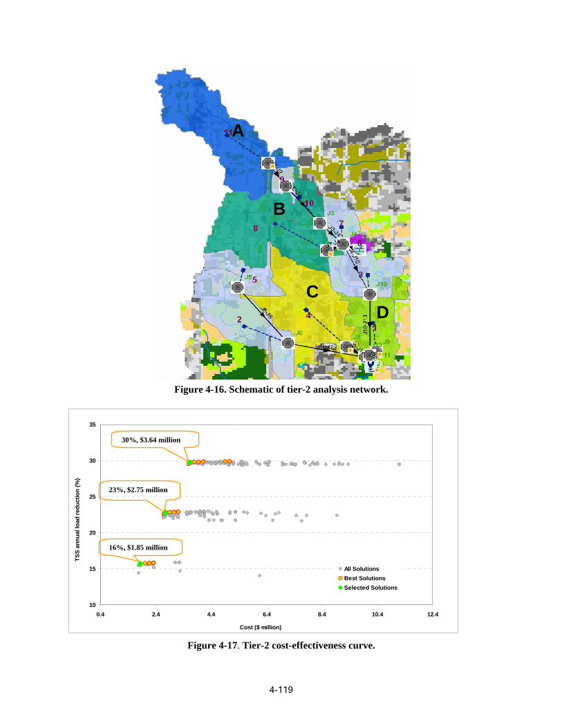
A

B

C D

35

30%, $3.64 million

30

23%, $2.75 million 25

20

16%, $1.85 million

15 All Solutions Best Solutions Selected Solutions

10 0.4 2.4 4.4 6.4 8.4 10.4 12.4

Cost ($ million)

TSS

annu

al lo

ad re

duct

i on

(%)

Figure 4-16. Schematic of tier-2 analysis network.

Figure 4-17. Tier-2 cost-effectiveness curve.

4-119

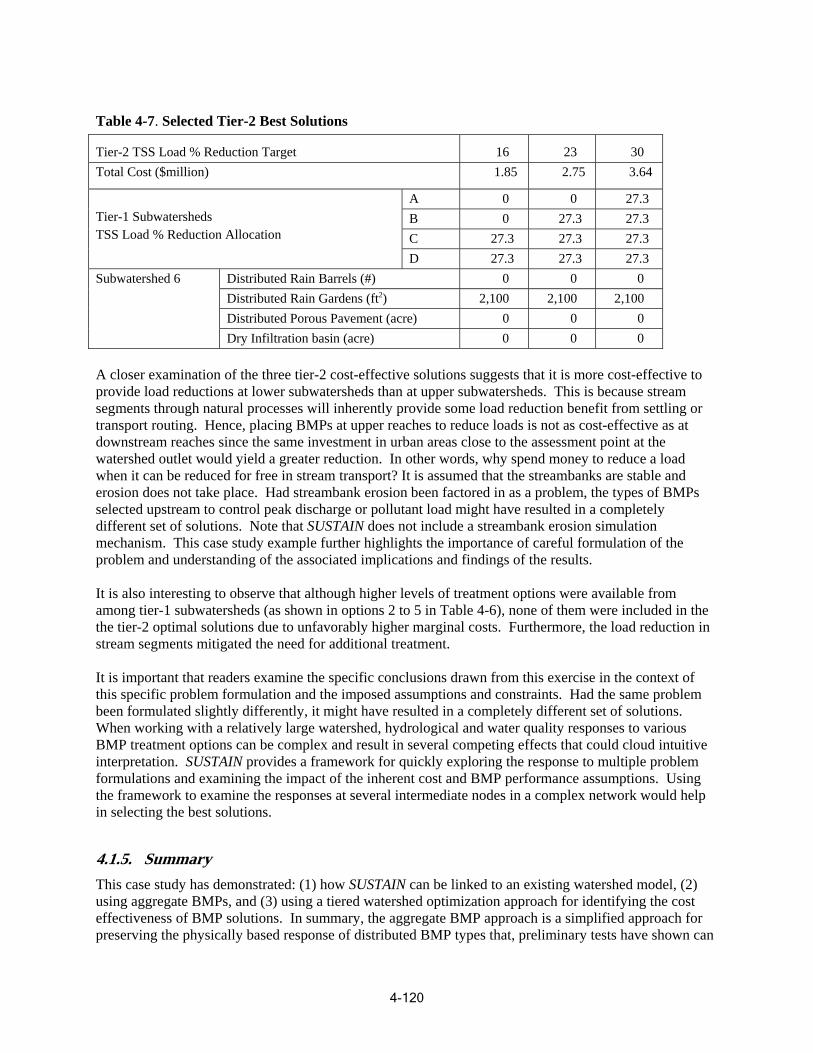
Table 4-7. Selected Tier-2 Best Solutions

Tier-2 TSS Load % Reduction Target 16 23 30 Total Cost ($million) 1.85 2.75 3.64

Tier-1 Subwatersheds SS Load % Reduction Allocation T

A 0 0 27.3 B 0 27.3 27.3 C 27.3 27.3 27.3 D 27.3 27.3 27.3

Subwatershed 6 Distributed Rain Barrels (#) 0 0 0 Distributed Rain Gardens (ft2) 2,100 2,100 2,100 Distributed Porous Pavement (acre) 0 0 0 Dry Infiltration basin (acre) 0 0 0

A closer examination of the three tier-2 cost-effecti ve solutions suggests that it is more cost-effective to provide load reductions at lower subwatersheds t han at upper subw atersheds. This is because stream segments through natural processes will inherently provide some load reduction benefit from settling or transport routing. Hence, placing BMPs at upper reaches to reduce loads is not as cost-effective as at downstream reaches since the same investment in urban areas close to the ass essment point at the watershed outlet would yield a greater reduction. In other words, why spend mo ney to reduce a load when it can be reduced for free in stream tra nsport? It is a ssumed that the strea mbanks are stable and erosion does not take place. Had streambank erosion been factored in as a problem, the types of BMPs selected upstream to control peak discharge or pollutant load might have resulted in a completely different set of solutions. Note that SUSTAIN does not include a streambank erosion simulation mechanism. This case study example further highlights the importance of careful formulation of the problem and understanding of the associated implications and findings of the results.

It is also interesting to observe that although higher levels of treatment options were available from among tier-1 subwatersheds (as shown in options 2 to 5 in Table 4-6), none of them were included in the the tier-2 optimal solutions due to unfavorably higher marginal costs. Furthermore, the load reduction in stream segments mitigated the need for additional treatment.

It is impo rtant that readers examine the specific conclusions drawn from this exercise in the context of this specific problem formulation and the imposed assumptions and constraints. Had the same problem been formulated slightly differently, it might have resulted in a completely different set of solutions. When working with a relatively large watershed, hy drological an d wat er quality responses to various BMP treatment opt ions can be complex and result in several com petin g effects that could cloud intuitive interpretation. SUSTAIN provides a framework for quickly expl oring the response to multiple problem formulations and examining the im pact of th e inher ent cost and BMP performance as sumpti ons. Using the framework to examine the resp onses at several intermediate nodes in a complex network would help in selecting the best solutions.

4.1.5. Summary This case study has demonstrated: (1) how SUSTAIN can be linked to an existing watershed model, (2) using aggregate BMPs, and (3) using a tiered watershed optimization approach for identifying the cost effectiveness of BMP solutions. In summary, the aggregate BMP approach is a simplified approach for preserving the physically based response of distributed BMP types that, preliminary tests have shown can

4-120

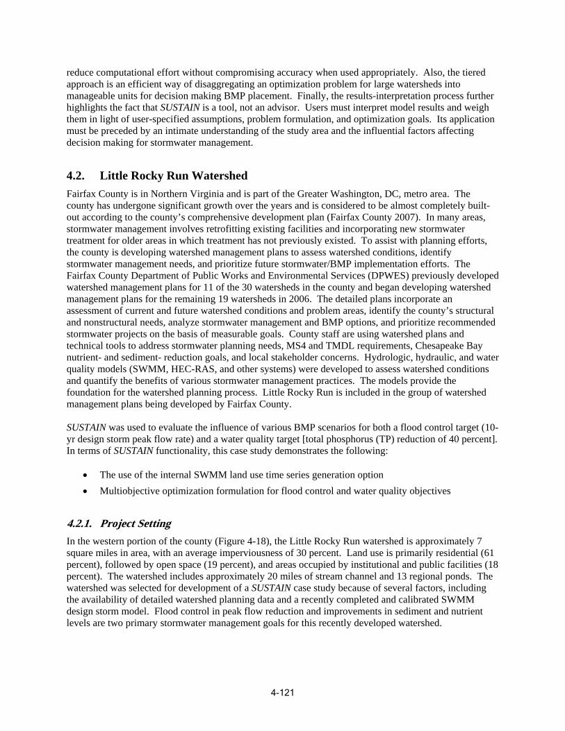
reduce computational effort without compromising accuracy when used appropriately. Also, the tiered approach is an efficient way of disaggregating an optimization problem for large watersheds into manageable units for decision making BMP placement. Finally, the results-interpretation process further highlights the fact that SUSTAIN is a tool, not an advisor. Users must interpret model results and weigh them in light of user-specified assumptions, problem formulation, and optimization goals. Its application must be preceded by an intimate understanding of the study area and the influential factors affecting decision making for stormwater management.

4.2. Little Rocky Run Watershed Fairfax County is in Northern Virginia and is part of the Greater Washington, DC, metro area. The county has undergone significant growth over the years and is considered to be almost completely built-out according to the county’s comprehensive development plan (Fairfax County 2007). In many areas, stormwater management involves retrofitting existing facilities and incorporating new stormwater treatment for older areas in which treatment has not previously existed. To assist with planning efforts, the county is developing watershed management plans to assess watershed conditions, identify stormwater management needs, and prioritize future stormwater/BMP implementation efforts. The Fairfax County Department of Public Works and Environmental Services (DPWES) previously developed watershed management plans for 11 of the 30 watersheds in the county and began developing watershed management plans for the remaining 19 watersheds in 2006. The detailed plans incorporate an assessment of current and future watershed conditions and problem areas, identify the county’s structural and nonstructural needs, analyze stormwater management and BMP options, and prioritize recommended stormwater projects on the basis of measurable goals. County staff are using watershed plans and technical tools to address stormwater planning needs, MS4 and TMDL requirements, Chesapeake Bay nutrient- and sediment- reduction goals, and local stakeholder concerns. Hydrologic, hydraulic, and water quality models (SWMM, HEC-RAS, and other systems) were developed to assess watershed conditions and quantify the benefits of various stormwater management practices. The models provide the foundation for the watershed planning process. Little Rocky Run is included in the group of watershed management plans being developed by Fairfax County.

SUSTAIN was used to evaluate the influence of various BMP scenarios for both a flood control target (10­yr design storm peak flow rate) and a water quality target [total phosphorus (TP) reduction of 40 percent]. In terms of SUSTAIN functionality, this case study demonstrates the following:

• The use of the internal SWMM land use time series generation option • Multiobjective optimization formulation for flood control and water quality objectives

4.2.1. Project Setting In the western portion of the county (Figure 4-18), the Little Rocky Run watershed is approximately 7 square miles in area, with an average imperviousness of 30 percent. Land use is primarily residential (61 percent), followed by open space (19 percent), and areas occupied by institutional and public facilities (18 percent). The watershed includes approximately 20 miles of stream channel and 13 regional ponds. The watershed was selected for development of a SUSTAIN case study because of several factors, including the availability of detailed watershed planning data and a recently completed and calibrated SWMM design storm model. Flood control in peak flow reduction and improvements in sediment and nutrient levels are two primary stormwater management goals for this recently developed watershed.

4-121

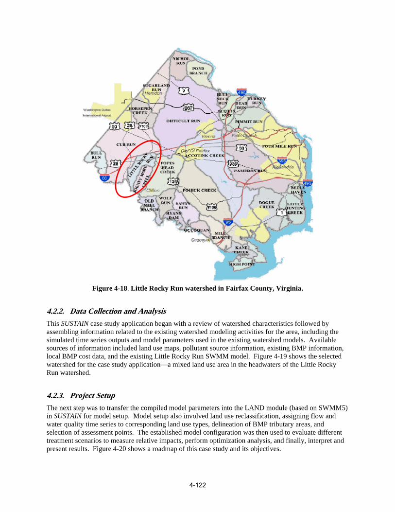
Figure 4-18. Little Rocky Run watershed in Fairfax County, Virginia.

4.2.2. Data Collection and Analysis This SUSTAIN case study application began with a review of watershed characteristics followed by assembling information related to the existing watershed modeling activities for the area, including the simulated time series outputs and model parameters used in the existing watershed models. Available sources of information included land use maps, pollutant source information, existing BMP information, local BMP cost data, and the existing Little Rocky Run SWMM model. Figure 4-19 shows the selected watershed for the case study application—a mixed land use area in the headwaters of the Little Rocky Run watershed.

4.2.3. Project Setup The next step was to transfer the compiled model parameters into the LAND module (based on SWMM5) in SUSTAIN for model setup. Model setup also involved land use reclassification, assigning flow and water quality time series to corresponding land use types, delineation of BMP tributary areas, and selection of assessment points. The established model configuration was then used to evaluate different treatment scenarios to measure relative impacts, perform optimization analysis, and finally, interpret and present results. Figure 4-20 shows a roadmap of this case study and its objectives.

4-122

   

     

          

        

              

 

      

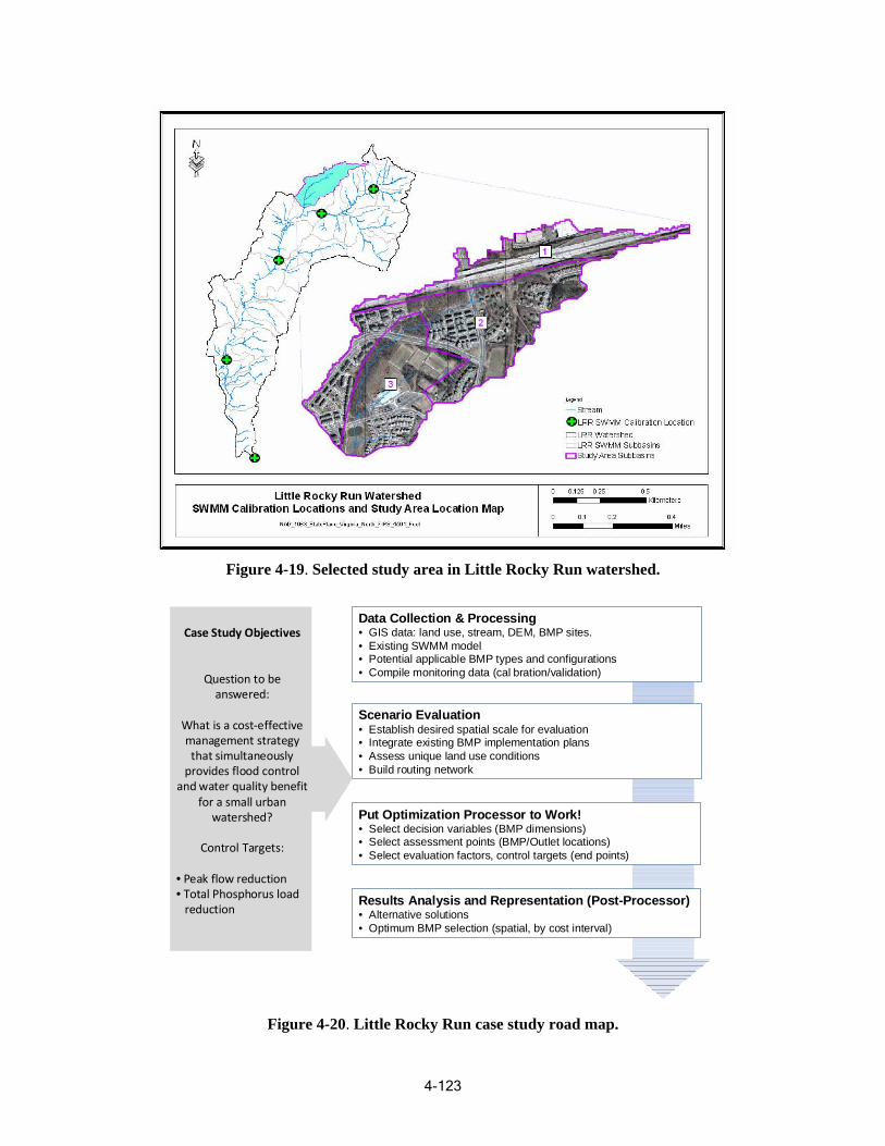
Figure 4-19. Selected study area in Little Rocky Run watershed.

Results Analysis and Representation (Post-Processor) • Alternative solutions • Optimum BMP selection (spatial, by cost interval)

Put Optimization Processor to Work! • Select decision variables (BMP dimensions) • Select assessment points (BMP/Outlet locations) • Select evaluation factors, control targets (end points)

Scenario Evaluation • Establish desired spatial scale for evaluation • Integrate existing BMP implementation plans • Assess unique land use conditions • Build routing network

Data Collection & Processing • GIS data: land use, stream, DEM, BMP sites. • Existing SWMM model • Potential applicable BMP types and configurations • Compile monitoring data (cal bration/validation)

Case Study Objectives

Question to be answered:

What is a cost‐effective management strategy that simultaneously provides flood control

and water quality benefit for a small urban

watershed?

Control Targets:

• Peak flow reduction • Total Phosphorus load reduction

Figure 4-20. Little Rocky Run case study road map.

4-123

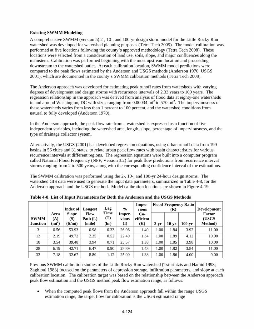
Existing SWMM Modeling A comprehensive SWMM (version 5) 2-, 10-, and 100-yr design storm model for the Little Rocky Run watershed was developed for watershed planning purposes (Tetra Tech 2009). The model calibration was performed at five locations following the county’s approved methodology (Tetra Tech 2008). These locations were selected from a consideration of land use, soils, slope, and major confluences along the mainstem. Calibration was performed beginning with the most upstream location and proceeding downstream to the watershed outlet. At each calibration location, SWMM model predictions were compared to the peak flows estimated by the Anderson and USGS methods (Anderson 1970; USGS 2001), which are documented in the county’s SWMM calibration methods (Tetra Tech 2008).

The Anderson approach was developed for estimating peak runoff rates from watersheds with varying degrees of development and design storms with recurrence intervals of 2.33 years to 100 years. The regression relationship in the approach was derived from analysis of flood data at eighty-one watersheds in and around Washington, DC with sizes ranging from 0.00034 mi2 to 570 mi2. The imperviousness of these watersheds varies from less than 1 percent to 100 percent, and the watershed conditions from natural to fully developed (Anderson 1970).

In the Anderson approach, the peak flow rate from a watershed is expressed as a function of five independent variables, including the watershed area, length, slope, percentage of imperviousness, and the type of drainage collector system.

Alternatively, the USGS (2001) has developed regression equations, using urban runoff data from 199 basins in 56 cities and 31 states, to relate urban peak flow rates with basin characteristics for various recurrence intervals at different regions. The regression equations were built into a computer program called National Flood Frequency (NFF, Version 3.2) for peak flow predictions from recurrence interval storms ranging from 2 to 500 years, along with the corresponding confidence interval of the estimations.

The SWMM calibration was performed using the 2-, 10-, and 100-yr 24-hour design storms. The watershed GIS data were used to generate the input data parameters, summarized in Table 4-8, for the Anderson approach and the USGS method. Model calibration locations are shown in Figure 4-19.

Table 4-8. List of Input Parameters for Both the Anderson and the USGS Methods

SWMM Junction

Area (A)

(mi2)

Index of Slope

(S) (ft/mi)

Longest Flow

Path (L) (mile)

Lag Time (T) (hr)

% Imper-vious

(I)

Imper-vious Co-

efficient (K)

Flood-Frequency Ratio (R) Development

Factor (USGS

Method) 2-yr 10-yr 100-yr 3 0.56 53.93 0.98 0.33 26.96 1.40 1.00 1.84 3.92 11.00

13 2.19 49.72 2.35 0.52 22.40 1.34 1.00 1.89 4.12 10.00 18 3.54 39.48 3.94 0.71 25.57 1.38 1.00 1.85 3.98 10.00 28 6.19 42.71 6.47 0.90 28.89 1.43 1.00 1.82 3.84 11.00 32 7.18 32.67 8.89 1.12 25.00 1.38 1.00 1.86 4.00 9.00

Previous SWMM calibration studies of the Little Rocky Run watershed (Tsihrintzis and Hamid 1998; Zaghloul 1983) focused on the parameters of depression storage, infiltration parameters, and slope at each calibration location. The calibration target was based on the relationship between the Anderson approach peak flow estimation and the USGS method peak flow estimation range, as follows:

• When the computed peak flows from the Anderson approach fall within the range USGS estimation range, the target flow for calibration is the USGS estimated range

4-124

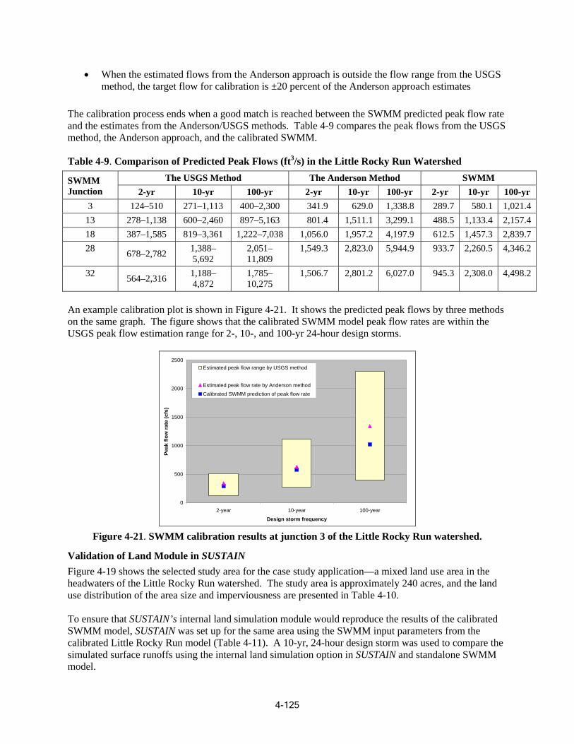
• When the estimated flows from the Anderson approach is outside the flow range from the USGS method, the target flow for calibration is ±20 percent of the Anderson approach estimates

The calibration process ends when a good match is reached between the SWMM predicted peak flow rate and the estimates from the Anderson/USGS methods. Table 4-9 compares the peak flows from the USGS method, the Anderson approach, and the calibrated SWMM.

Table 4-9. Comparison of Predicted Peak Flows (ft3/s) in the Little Rocky Run Watershed

SWMM The USGS Method The Anderson Method SWMM Junction 2-yr 10-yr 100-yr 2-yr 10-yr 100-yr 2-yr 10-yr 100-yr

3 124–510 271–1,113 400–2,300 341.9 629.0 1,338.8 289.7 580.1 1,021.4 13 278–1,138 600–2,460 897–5,163 801.4 1,511.1 3,299.1 488.5 1,133.4 2,157.4 18 387–1,585 819–3,361 1,222–7,038 1,056.0 1,957.2 4,197.9 612.5 1,457.3 2,839.7 28 678–2,782 1,388–

5,692 2,051– 11,809

1,549.3 2,823.0 5,944.9 933.7 2,260.5 4,346.2

32 564–2,316 1,188– 4,872

1,785– 10,275

1,506.7 2,801.2 6,027.0 945.3 2,308.0 4,498.2

An example calibration plot is shown in Figure 4-21. It shows the predicted peak flows by three methods on the same graph. The figure shows that the calibrated SWMM model peak flow rates are within the USGS peak flow estimation range for 2-, 10-, and 100-yr 24-hour design storms.

0

500

1000

1500

2000

2500

2-year 10-year 100-year

Design storm frequency

Peak

flow

rate

(cfs

)

Estimated peak flow range by USGS method

Estimated peak flow rate by Anderson method

Calibrated SWMM prediction of peak flow rate

Figure 4-21. SWMM calibration results at junction 3 of the Little Rocky Run watershed.

Validation of Land Module in SUSTAIN Figure 4-19 shows the selected study area for the case study application—a mixed land use area in the headwaters of the Little Rocky Run watershed. The study area is approximately 240 acres, and the land use distribution of the area size and imperviousness are presented in Table 4-10.

To ensure that SUSTAIN’s internal land simulation module would reproduce the results of the calibrated SWMM model, SUSTAIN was set up for the same area using the SWMM input parameters from the calibrated Little Rocky Run model (Table 4-11). A 10-yr, 24-hour design storm was used to compare the simulated surface runoffs using the internal land simulation option in SUSTAIN and standalone SWMM model.

4-125

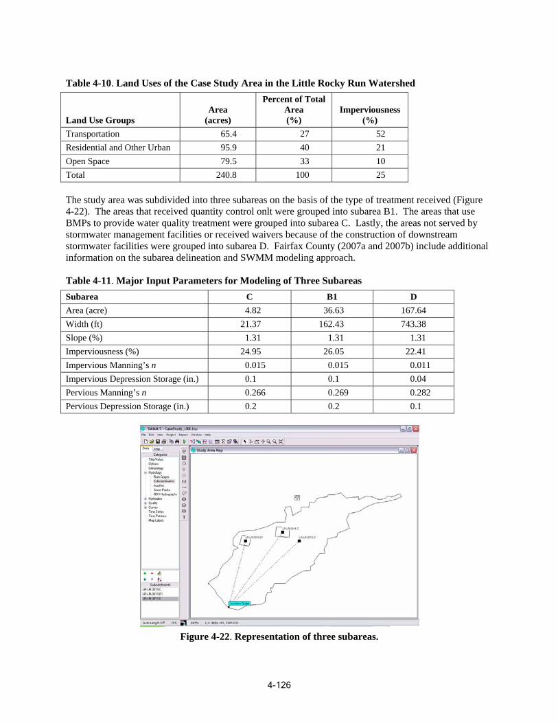
Table 4-10. Land Uses of the Case Study Area in the Little Rocky Run Watershed

Land Use Groups Area

(acres)

Percent of Total Area (%)

Imperviousness (%)

Transportation 65.4 27 52 Residential and Other Urban 95.9 40 21 Open Space 79.5 33 10 Total 240.8 100 25

The study area was subdivided into three subareas on the basis of the type of treatment received (Figure 4-22). The areas that received quantity control onlt were grouped into subarea B1. The areas that use BMPs to provide water quality treatment were grouped into subarea C. Lastly, the areas not served by stormwater management facilities or received waivers because of the construction of downstream stormwater facilities were grouped into subarea D. Fairfax County (2007a and 2007b) include additional information on the subarea delineation and SWMM modeling approach.

Table 4-11. Major Input Parameters for Modeling of Three Subareas Subarea C B1 D Area (acre) 4.82 36.63 167.64 Width (ft) 21.37 162.43 743.38 Slope (%) 1.31 1.31 1.31 Imperviousness (%) 24.95 26.05 22.41 Impervious Manning’s n 0.015 0.015 0.011 Impervious Depression Storage (in.) 0.1 0.1 0.04 Pervious Manning’s n 0.266 0.269 0.282 Pervious Depression Storage (in.) 0.2 0.2 0.1

Figure 4-22. Representation of three subareas.

4-126

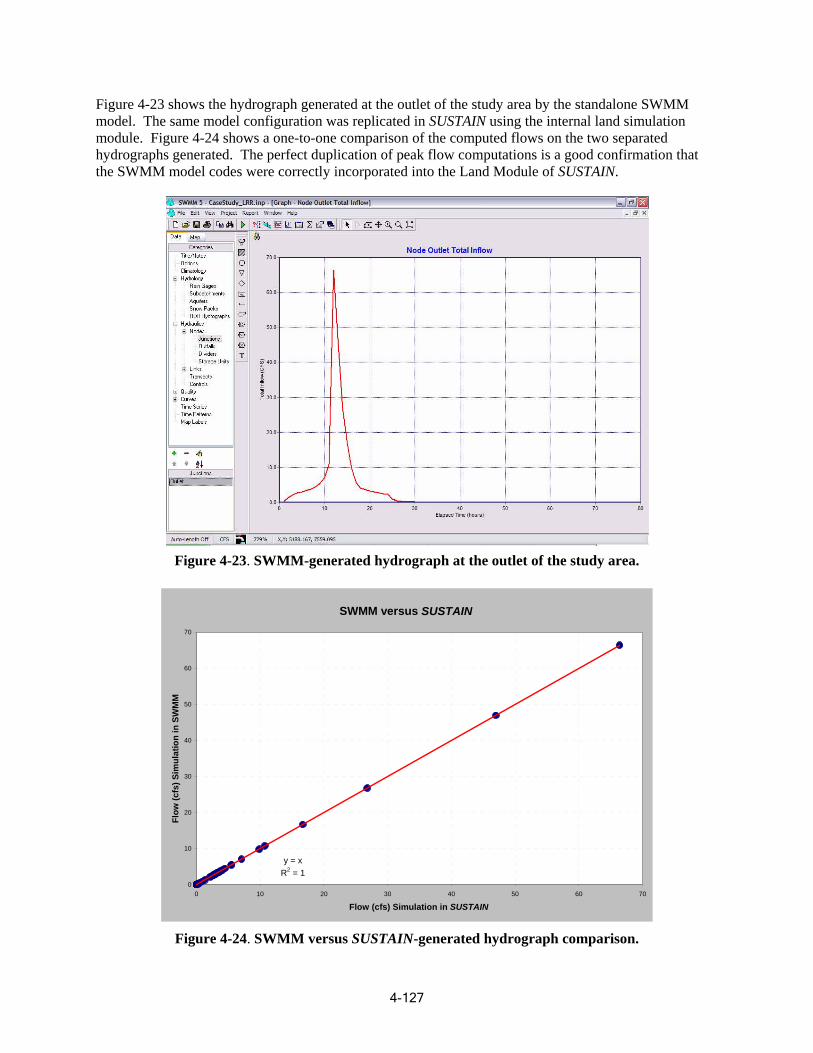
Figure 4-23 shows the hydrograph generated at the outlet of the study area by the standalone SWMM model. The same model configuration was replicated in SUSTAIN using the internal land simulation module. Figure 4-24 shows a one-to-one comparison of the computed flows on the two separated hydrographs generated. The perfect duplication of peak flow computations is a good confirmation that the SWMM model codes were correctly incorporated into the Land Module of SUSTAIN.

Figure 4-23. SWMM-generated hydrograph at the outlet of the study area.

SWMM versus SUSTAIN

Flow

(cfs

) Sim

ulat

ion

in S

W M

M

70

60

50

40

30

20

10

0

y = x R2 = 1

0 10 20 30 40 50 60 70

Flow (cfs) Simulation in SUSTAIN

Figure 4-24. SWMM versus SUSTAIN-generated hydrograph comparison.

4-127

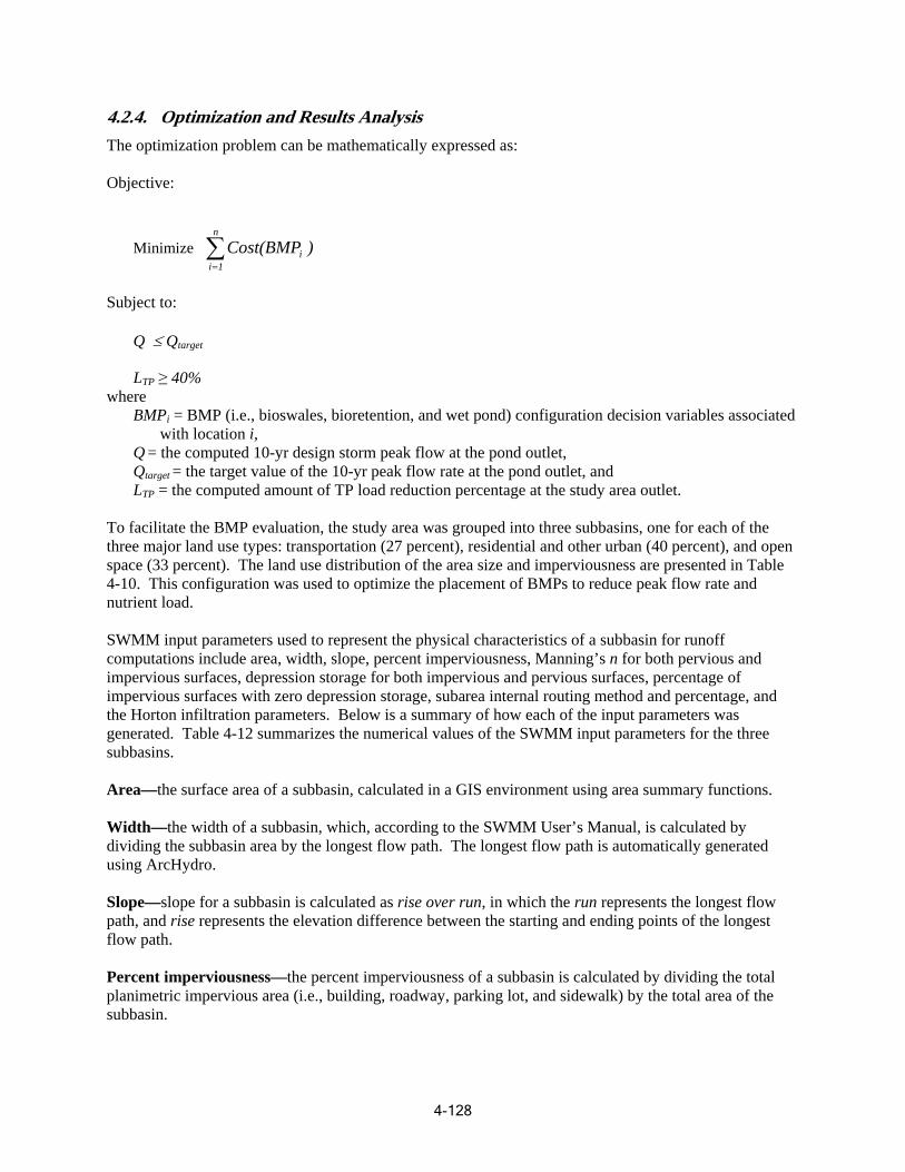
4.2.4. Optimization and Results Analysis The optimization problem can be mathematically expressed as:

Objective:

n

Minimize ∑Cost(BMPi ) i=1

Subject to:

Q ≤ Qtarget

LTP ≥ 40% where

BMPi = BMP (i.e., bioswales, bioretention, and wet pond) configuration decision variables associated with location i,

Q = the computed 10-yr design storm peak flow at the pond outlet, Qtarget = the target value of the 10-yr peak flow rate at the pond outlet, and LTP = the computed amount of TP load reduction percentage at the study area outlet.

To facilitate the BMP evaluation, the study area was grouped into three subbasins, one for each of the three major land use types: transportation (27 percent), residential and other urban (40 percent), and open space (33 percent). The land use distribution of the area size and imperviousness are presented in Table 4-10. This configuration was used to optimiz e the placement of BMPs to reduce peak flow rate and nutrient load.

SWMM input parameters used to represent the physical characteristics of a subbasin for runoff computations include area, width, slope, percent imperviousness, Manning’s n for both pervious and im pervious surfaces, depression storage for both impervious and pervious surfaces, percentage of impervious surfaces with zero depression storage, subarea internal routing method and percentage, and the Horton infiltration parameters. Below is a summary of how e ach of the input parameters was generated. Table 4-12 summarizes the numerical values of the SWMM input parameters for the three subbasins.

Area—the surface area of a subbasin, calculated in a GIS environment using area summ ary f unctions.

Width—the width of a subbasin, which, according to the SWMM User’s Manual, is calculated by dividing the subbasin area b y the longest flow path. The longest flow path is automatically generated using ArcHydro.

Slope—slope for a subbasin is calculated as rise over run, in which the run represents the longest flow path, and rise represents the elevation difference between the starting and ending points of the longest flow path.

Percent imperviousness—the percent imperviousness of a subbasin is calculated by dividing the total planimetric impervious area (i.e., building, roadway, parking lot, and sidewalk) by the total area of the subbasin.

4-128

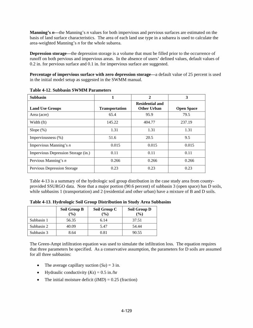
Manning’s n—the Manning’s n values for both impervious and pervious surfaces are estimated on the basis of land surface characteristics. The area of each land use type in a subarea is used to calculate the area-weighted Manning’s n for the whole subarea.

Depression storage—the depression storage is a volume that must be filled prior to the occurrence of runoff on both pervious and impervious areas. In the absence of users’ defined values, default values of 0.2 in. for pervious surface and 0.1 in. for impervious surface are suggested.

Percentage of impervious surface with zero depression storage—a default value of 25 percent is used in the initial model setup as suggested in the SWMM manual.

Table 4-12. Subbasin SWMM Parameters Subbasin 1 2 3

Land Use Groups Transportation Residential and

Other Urban Open Space Area (acre) 65.4 95.9 79.5

Width (ft) 145.22 404.77 237.19

Slope (%) 1.31 1.31 1.31

Imperviousness (%) 51.6 20.5 9.5

Impervious Manning’s n 0.015 0.015 0.015

Impervious Depression Storage (in.) 0.11 0.11 0.11

Pervious Manning’s n 0.266 0.266 0.266

Pervious Depression Storage 0.23 0.23 0.23

Table 4-13 is a summary of the hydrologic soil group distribution in the case study area from county-provided SSURGO data. Note that a major portion (90.6 percent) of subbasin 3 (open space) has D soils, while subbasins 1 (transportation) and 2 (residential and other urban) have a mixture of B and D soils.

Table 4-13. Hydrologic Soil Group Distribution in Study Area Subbasins Soil Group B

(%) Soil Group C

(%) Soil Group D

(%) Subbasin 1 56.35 6.14 37.51 Subbasin 2 40.09 5.47 54.44 Subbasin 3 8.64 0.81 90.55

The Green-Ampt infiltration equation was used to simulate the infiltration loss. The equation requires that three parameters be specified. As a conservative assumption, the parameters for D soils are assumed for all three subbasins:

• The average capillary suction (Su) = 3 in. • Hydraulic conductivity (Ks) = 0.5 in./hr • The initial moisture deficit (IMD) = 0.25 (fraction)

4-129

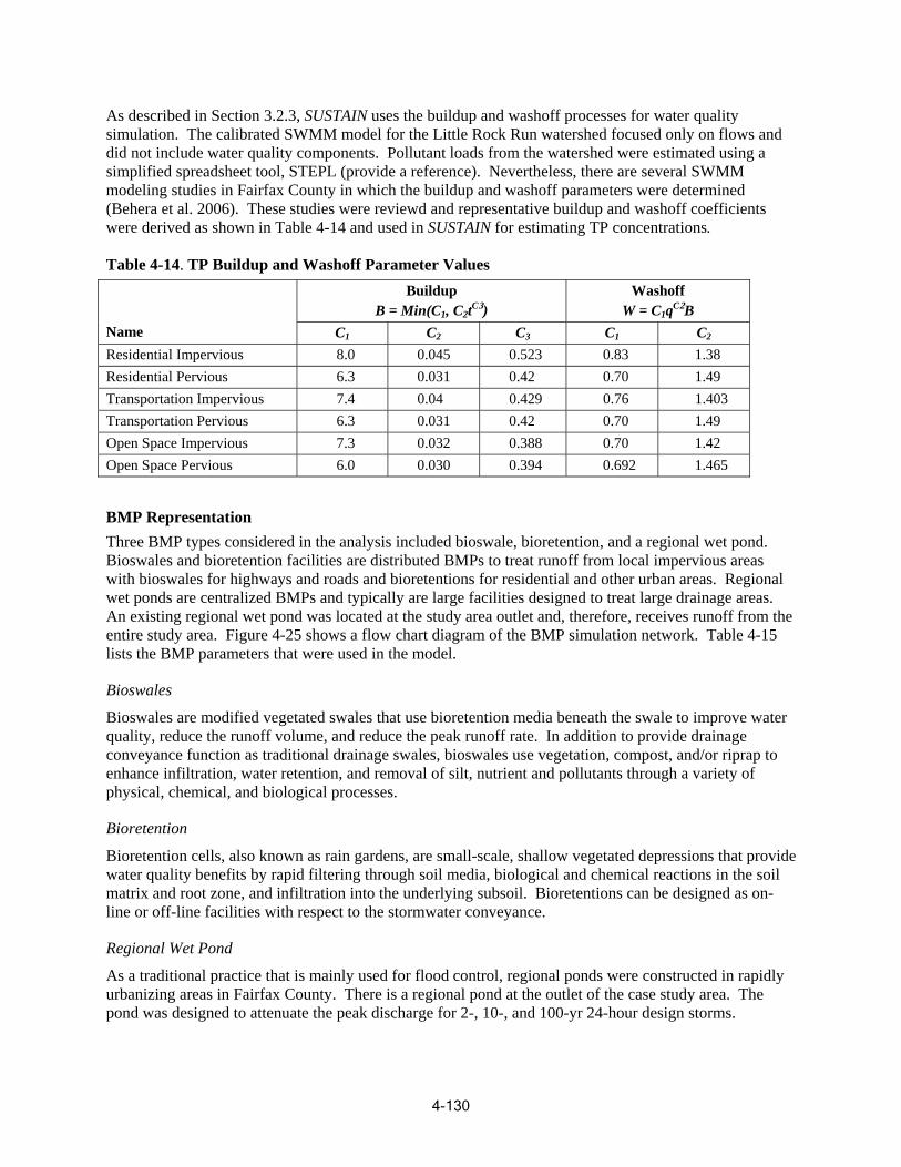
As described in Section 3.2.3, SUSTAIN uses the buildup and washoff processes for water quality simulation. The calibrated SWMM model for the Little Rock Run watershed focused only on flows and did not include water quality components. Pollutant loads from the watershed were estimated using a simplified spreadsheet tool, STEPL (provide a reference). Nevertheless, there are several SWMM modeling studies in Fairfax County in which the buildup and washoff parameters were determined (Behera et al. 2006). These studies were reviewd and representative buildup and washoff coefficients were derived as shown in Table 4-14 and used in SUSTAIN for estimati ng TP concentrations.

Table 4-14. TP Buildup and Washoff Parameter Values

Name

Buildup B = Min(C1, C2tC3)

Washoff W = C1qC2B

C1 C2 C3 C1 C2

Residential Impervious 8.0 0.045 0.523 0.83 1.38 Residential Pervious 6.3 0.031 0.42 0.70 1.49 Transportation Impervious 7.4 0.04 0.429 0.76 1.403 Transportation Pervious 6.3 0.031 0.42 0.70 1.49 O spen Space Imperviou 7.3 0.032 0.388 0.70 1.42 Open Space Pervious 6.0 0.030 0.394 0.692 1.465

BMP Representation Three BMP types considered in the analysis included bioswale, bioretention, and a regional wet pond. Bioswales and bioretention facilities are distributed BMPs to treat runoff from local impervious areas with bioswales for highways and roads and bioretentions for residential and other urban areas. Regional wet ponds are centralized BMPs and typically are large facilities designed to treat large drainage areas. An existing regional wet pond was located at the study area outlet and, therefore, receives runoff from the entire study area. Figure 4-25 shows a flow chart diagram of the BMP simulation network. Table 4-1 5 lists the BMP parameters that were used in the model.

Bioswales

Bioswales are modified vegetated swales that use bioretention media beneath the swale to improve water quality, reduce the runoff volume, and reduce the peak runoff rate. In addition to provide drainage conveyance function as traditional drainage swales, bioswales use vegetation, compost, and/or riprap to enhance infiltration, water retention, and removal of silt, nutrient and pollutants through a variety of physical, chemical, and biological processes.

Bioretention

Bioretention cells, also known as rain gardens, are small-scale, shallow vegetated depressions that provide water quality benefits by rapid filtering through soil media, biological and chemical reactions in the soil matrix and root zone, and infiltration into the underlying subsoil. Bioretentions can be designed as on­line or off-line facilities with respect to the stormwater conveyance.

Regional Wet Pond

As a traditional practice that is mainly used for flood control, regional ponds were constructed in rapidly urbanizing areas in Fairfax County. There is a regional pond at the outlet of the case study area. The pond was designed to attenuate the peak discharge for 2-, 10-, and 100-yr 24-hour design storms.

4-130

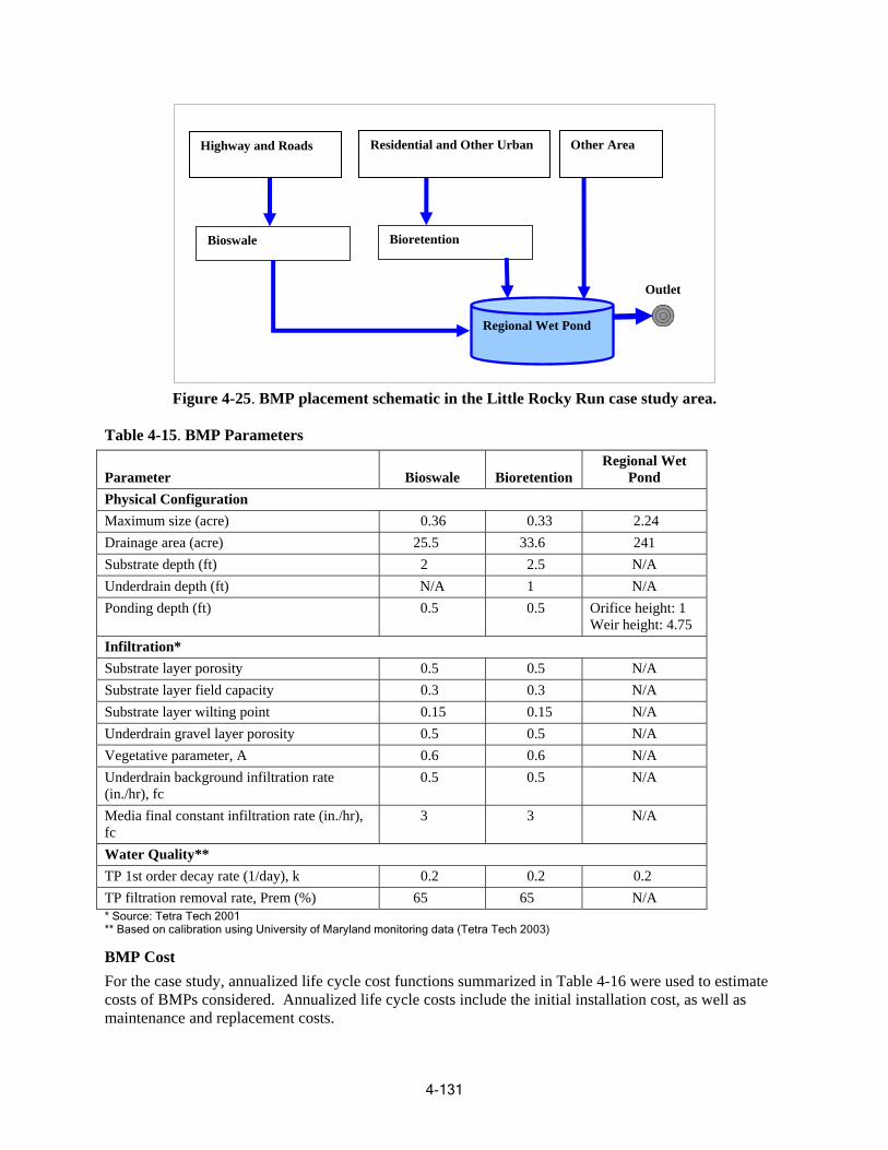
Regional Wet Pond

Outlet

Other Area

Bioretention Bioswale

Residential and Other Urban Highway and Roads

Figure 4-25. BMP placement schematic in the Little Rocky Run case study area.

Table 4-15. BMP Parameters

Parameter Bioswale Bioretention Pond Regional Wet

Physical Configuration Maximum size (acre) 0.36 0.33 2.24 Drainage area (acre) 25.5 33.6 241 Substrate depth (ft) 2 2.5 N/A Underdrain depth (ft) N/A 1 N/A Ponding depth (ft) 0.5 0.5

Weir height: 4.75 Orifice height: 1

Infiltration* Substrate layer porosity 0.5 0.5 N/A Substrate layer field capacity 0.3 0.3 N/A Substrate layer wilting point 0.15 0.15 N/A Underdrain gravel layer porosity 0.5 0.5 N/A Vegetative parameter, A 0.6 0.6 N/A Underdrain background infiltration rate (in./hr), fc

0.5 0.5 N/A

Media fi n rate (in./hr), nal constant infiltratio fc

3 3 N/A

Water Quality** TP 1st o rder decay rate (1/day), k 0.2 0.2 0.2 TP filtration removal rate, Prem (%) 65 65 N/A * Source: Tetra Tech 2001 ** Based on calibration using University of Maryland monitoring data (Tetra Tech 2003)

BMP Cost For the case study, annualized life cycle cost functions summarized in Table 4-16 were used to estimate costs of BMPs considered. Annualized life cycle costs include the initial installation cost, as well as maintenance and replacement costs.

4-131

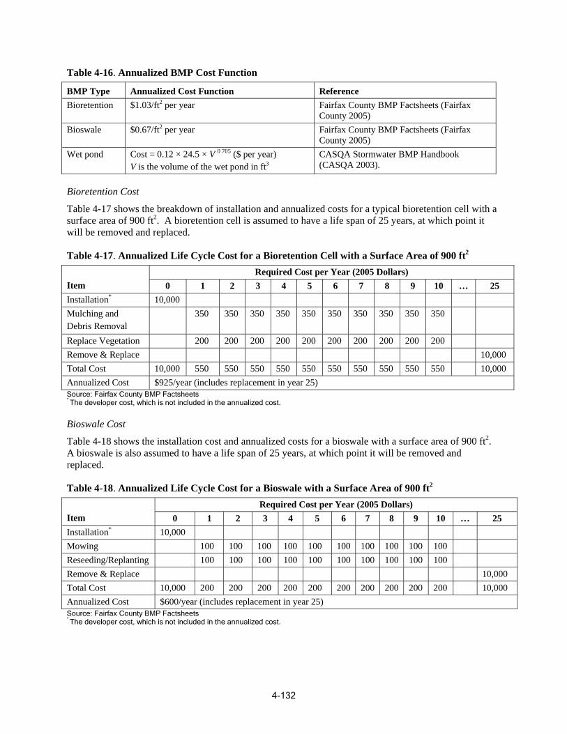
Table 4-16. Annualized BMP Cost Function

peBMP Ty Annualized Cost Function Reference Bioretention $1.03/ft2 per year Fairfax County BMP Factsheets (Fairfax

County 2005) Bioswale $0.67/ft2 per year Fairfax County BMP Factsheets (Fairfax

County 2005) Wet pond Cost = 0.12 × 24.5 × V 0 705 ($ per year)

V is the volume of the wet pond in ft3 CASQA Stormwater BMP Handbook (CASQA 2003).

Bioretention Cost

Table 4-17 shows the breakdown of installation and annualized costs for a typical bioretention cell w ith a surface area of 900 ft 2. A bioretention cell is assumed to have a life span of 25 years, at which point it will be removed and replaced.

Table 4-17. Annualized Life Cycle Cost for a Bioretention Cell with a Surface Area of 900 ft2

Item Required Cost per Year (2005 Dollars)

0 1 2 3 4 5 6 7 8 9 10 … 25 Installation* 10,000 Mulching and Debris Removal

350 350 350 350 350 350 350 350 350 350

Replace Vegetation 200 200 200 200 200 200 200 200 200 200 Remove & Replace 10,000 Total Co st 10,000 550 550 550 550 550 550 550 550 550 550 10,000 Annualized Cost $925/year (includes replacement in year 25) Source: Fairfax County BMP Factsheets * The developer cost, which is not included in the annualized cost.

Bioswale Cost

Table 4-18 shows the installation cost and annualized costs for a bioswale with a surface area of 900 ft2. A bioswale is also assumed to have a life span of 25 years, at which point it will be removed and replaced.

Table 4-18. Annualized Life Cycle Cost for a Bioswale with a Surface Area of 900 ft2

Item Required Cost per Year (2005 Dollars)

0 1 2 3 4 5 6 7 8 9 10 … 25 Installation* 10,000 Mowing 100 100 100 100 100 100 100 100 100 100 Reseeding/Replanting 100 100 100 100 100 100 100 100 100 100 Remove & Replace ,00010 Total Co st 10,000 200 200 200 200 200 200 200 200 200 200 10,000 Annualized Cost $600/year (includes replacement in year 25) Source: Fairfax County BMP Factsheets * The dev eloper cost, which is not included in the annualized cost.

4-132

Wet Pond Cost

Wet Pond costs were estimated as described below.

Construction Cost

Cost = 24.5 × V 0.705 (see Table 4-16) (4-1) where

Cost ($) = the cost for construction, design, and permitting, and V = volume of the wet pond in ft . 3

Converting the capital cost to annualized capital cost by assuming a 20-yr life span and 0.05 annual interest rate gives

Annualized Capital Cost ($/yr) = 0.08 × 24.5 × V 0.705 (4-2)

Maintenance Cost The mid-range of maintenance cost is approximated to be four percent of capital cost per year.

0.705 Annualized Maintenance Cost ($/yr) = 0.04 × 24.5 × V (4-3)

Annualized Life Cycle Cost (including capital and maintenanc e cost)

Annualized Cost = 0.12 × 24.5 × V 0.705 (see Table 4-16) (4-4) where

Annualized Cost ($) = the cost of construction, design, permitting, maintenance, and replacem ent, and V = the volume of the wet pond in ft3.

Simulation Period and Evaluation Factors As previously described, the objectives of this optimization case study are to provide flood control up to the 10-yr design storm and achieve a minimum of 40 percent reduction of TP load. Because of local water quality improvement needs and the ultimate downstream effect on the Chesapeake Bay, reduction in nutrient loading is an important objective for the stormwater ma nagement in Fairfax County. BMP effectiveness was measured at the designated assessment point at the study area outlet.

The use of continuous simulation provides modelers with an opportunity to capture the dynamic responses of BMPs under various storm conditions. However, among the large potential sets of data , it is often possible to identify one set of data that can reasonably represent either the long-term average treatment performance of BMPs or a critical condition that is most closely associated with the nature o f the problem being studied. From the analysis of precipitation data, the calendar year 1994 (January 1, 1994–December 31, 1994) was determined to be representative of average hydrologic conditions in the watershed. The total rainfall depth for the year was close to the 17-yr average of 43.3 in. In addition, both pre cipitation depth and intensity distribution were relatively close to the long-term statis tical average distribution. Figure 4-26 shows the average annual precipitation at th e Washington Dulles International Airport for calendar years 1990–2006.

As mentioned previously, calendar year 1994 had the most ty pical rainfall magnitude and intensity distribution from among the four highlighted years that were close to the 17-yr average. Figure 4-27 shows the rainfall volume and intensity distribution for wet intervals occurring in calendar year 1994 at

4-133

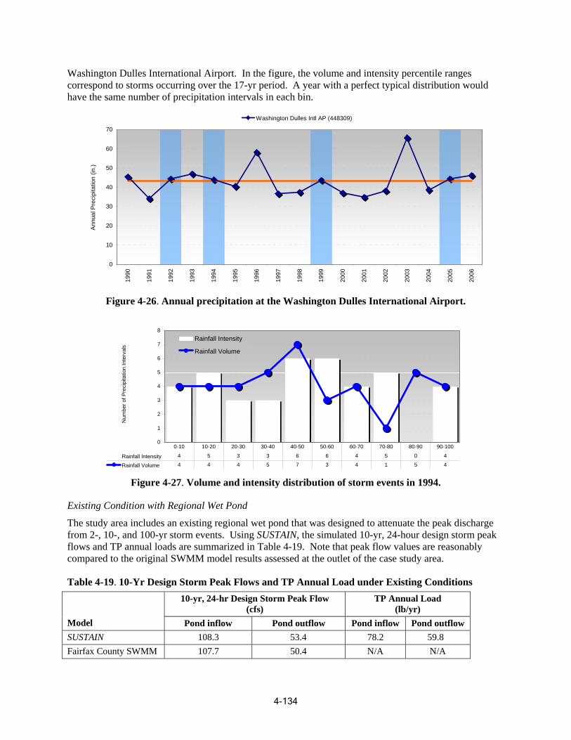
Washington Dulles International Airport. In the figure, the volume and intensity percentile ranges correspond to storms occurring over the 17-yr period. A year with a perfect typica l distribution would have the same number of precipitation intervals in each bin.

Washington Dulles Intl AP (448309)

0

10

20

30reci

p

40

50)

60

70

Ann

ual P

ita

tion

(in.

1990

1991

1992

1993

1994

1995

1996

1997

1998

1999

2000

2001

2002

2003

2004

2005

2006

Figure 4-26. Annual precipitation at the Washington Dulles International Airport.

Num

ber o

f Pre

cipi

tatio

n In

te rv

als

0

1

2

3

4

5

6

7

8 Rainfall Intensity

Rainfall Volume

Rainfall Intensity 4 5 3 3 6 6 4 5 0 4

Rainfall Volume 4 4 4 5 7 3 4 1 5 4

0-10 10-20 20-30 30-40 40-50 50-60 60-70 70-80 80-90 90-100

Figure 4-27. Volume and intensity distribution of storm events in 1994.

Existing Condition with Regional Wet Pond

The study area includes an existing regional w et pond that was designed to attenuate the peak discharge from 2-, 10-, and 100-yr storm events. Using SUSTAIN, the simulated 10-yr, 24-hour design storm p eak flows and TP annual loads are summarized in Table 4-19. Note that peak flow values are reasonably compar ed to the original SWMM model results assessed at the outlet of the case study area.

Table 4-19. 10-Yr Design Storm Peak Flows and TP Annual Load under Existing Conditions

Model

10-yr, 24-hr Design Storm Peak Flow (cfs)

TP Annual Load (lb/yr)

Pond inflow Pond outflow Pond inflow Pond outflow SUSTAI N 108.3 53.4 78.2 59.8 Fairfax County SWMM 107.7 50.4 N/A N/A

4-134

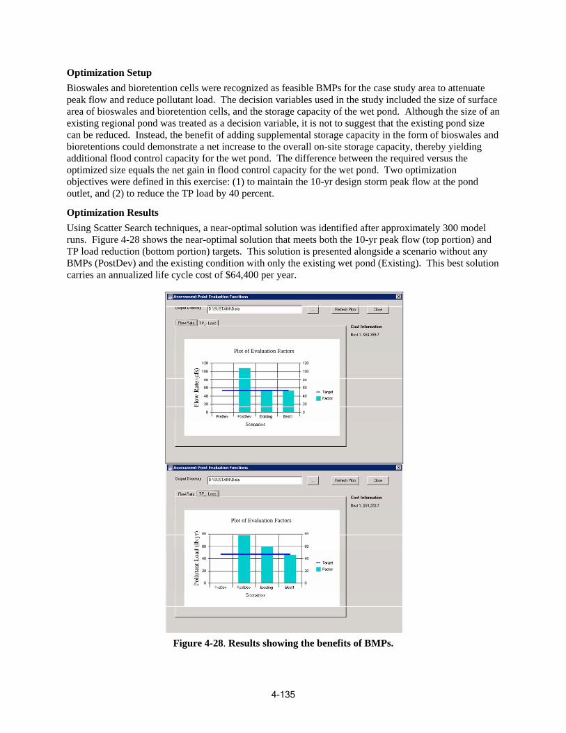
Plot of Evaluation Factors

Plot of Evaluation Factors

Figure 4-28. Results showing the benefits of BMPs.

Optimization Setup Bioswales and bioretention cells were recognized as feasible BMPs for the case study area to attenuate peak flow and reduce pollutant load. The decision variables used in the study included the size of surface area of bioswales and bioretention cells, and the storage capacity of the wet pond. Although the size of an existing regional pond was treated as a decision variable, it is not to suggest that the existing pond size can be reduced. Instead, the benefit of adding supplemental storage capacity in the form of bioswales and bioretentions could demonstrate a net increase to the overall on-site storage capacity, thereby yielding additional flood control capacity for the wet pond. The difference between the required versus the optimiz ed size equals the net gain in flood control capacity for the wet pond. Two optimization objectives were defined in this exercise: (1) to maintain the 10-yr design storm peak flow at the pond outlet, and (2) to reduce the TP load by 40 percent.

Optimization Results Using Scatter Search techniques, a near-optimal solution was identified after approximately 300 model runs. Figure 4-28 shows the near-optimal solution that meets both the 10-yr peak flow (top portion) andTP load reduction (bottom portion) targets. This solution is presented alongside a scenario witho ut any BMPs (PostDev) and the existing condition with only the existing wet pond (Existing). This best solution carries an annualized life cycle cost of $64,400 per year.

4-135

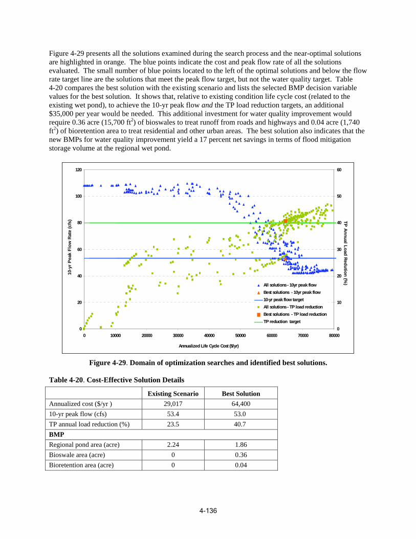
Figure 4-29 presents all the solutions examined during the search process and the near-optimal solutions are highlighted in orange. The blue points indicate the cost and peak flow rate of all the solutions evaluated. The small number of blue points located to the left of the optimal solutions and below the flow rate target line are the solutions that meet the peak flow target, but not the water quality target. Table 4-20 compares the best solution with the existing scenario and lists the selected BMP decision variable values for the best solution. It shows that, relative to existing condition life cycle cost (related to the existing wet pond), to achieve the 10-y r peak flow and the TP load reduction targets, an additional $35,000 per year would be needed. This additional investment for water quality improvement would require 0.36 acre (15,700 ft2) of bioswales to treat runoff from roads and highways and 0.04 acre (1,740 ft2) of bioretention area to treat residential and other urban areas. The best solution also indicates that the new BMPs for water quality improvement yield a 17 percent net savings in terms of flood mitigation storage volume at the regional wet pond.

0

20

80

100

120

e (c

fs)

40

50

60

4010-y

r P

60 Flo

w

30

0 10000 20000 30000 40000 50000 60000 70000 80000

eak

Rat

0

10

20

Annualized Life Cycle Cost ($/yr)

All solutions - 10yr peak flow Best solutions - 10yr peak flow 10-yr peak flow target All solutions - TP load reduction Best solutions - TP load reduction TP reduction target

TP A

nnua d R

on

l Loa eduti

(%)

Figure 4-29. Domain of optimization searches and identified best solutions.

Table 4-20. Cost-Effective Solution Details

Existing Scenario Best Solution Annualized cost ($/yr ) 29,017 64,400 10-yr peak flow (cfs) 53.4 53.0 TP annual load reduction (%) 23.5 40.7 BMP Regional pond area (acre) 2.24 1.86 Bioswale area (acre) 0 0.36 Bioretention area (acre) 0 0.04

4-136

4.2.5. Summary This case study has demonstrated: (1) a verification of the internal SWMM land module against the standalone SWMM 5 model and the use of the internal model to generate flow and pollutant loads from land, and (2) use of the Scatter Search optimization technique to find a near-optimal solution, given multiple control targets of peak flow and TP load reduction. Using optimization to guide decision making has been demonstrated to provide meaningful insights into the hydrologic response and benefits of BMPs for stormwater management. SUSTAIN is a powerful tool for decision-making. However, the outcomes from a SUSTAIN application would very much depend on the user-defined goals and assumptions. Hence, the results mus t be interpreted considering the use r-specified assumptions, problem formulation, and defined optimization constraints. As stated before, the SUSTAIN application must be accompanied byan intimate understanding of the study area and the identification of influential factors that affect the decision making to achieve stormwater management goals.

4-137

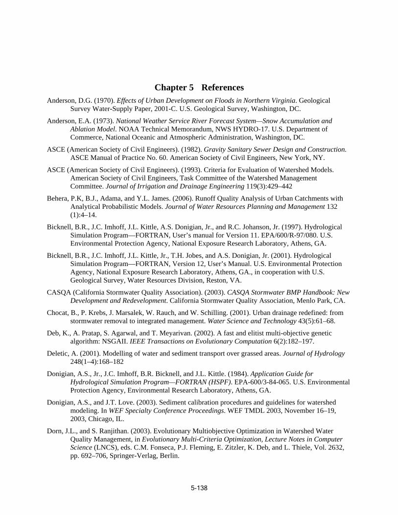
Chapter 5 References Anderson, D.G. (1970). Effects of Urban Development on Floods in North ern Virginia. Geological

p 01-C. U.S. Geological Survey, Wa shington, DC. Survey Water-Sup ly Paper, 20

Anderson, E.A. (1973). National Weather Service River Foreca st System—Snow Accumulation and Ablation Model. NOAA Technical Memorandum, NWS HYDRO-17. U.S. Departm ent of Commerce, National Oceanic and Atmospheric Administration, Washington, DC.

ASCE (American Society of Civil Engineers). (1982). Gravity Sanitary Sewer Design and Construction. ASCE Manual of Practice No. 60. American Society of Civil Engineers, New York, NY.

ASCE (American Society of Civil Engineers). (1993). Criteria for Evaluation of Watershed Models. American Society of Civil Engineers, Task Committee of the Watershed Management Committee. Journal of Irrigation and Drainage Engineering 119(3):429–442

Behera, P.K, B.J., Adama, and Y.L. James. (2006). Runoff Quality Analysis of Urban Catchments with Analytical Probabilistic Models. Journal of Water Resources Planning and Management 132 (1):4–14.

Bicknell, B.R., J.C. Imhoff, J.L. Kittle, A.S. Donigian, Jr., and R.C. Johanson, Jr. (1997). Hydrological Simulation Program—FORTRAN, User’s manual for Version 11. EPA/600/R-97/080. U.S. Environmental Protection Agency, National Exposure Research Laboratory, Athens, GA.

Bicknell, B.R., J.C. Imhoff, J.L. Kittle, Jr., T.H. Jobes, and A.S. Donigian, Jr. (2001). Hydrological Simulation Program—FORTRAN, Version 12, User’s Manual. U.S. Environmental Protection Agency, National Exposure Research Laboratory, Athens, GA., in cooperation with U.S. Geological Survey, Water Resources Division, Reston, VA.

CASQA (California Stormwater Quality Association). (2003). CASQA Stormwater BMP Handbook: New Development and Redevelopment. California Stormwater Quality Association, Menlo Park, CA.

Chocat, B., P. Krebs, J. Marsalek, W. Rauch, and W. Schilling. (2001). Urban drainage redefined: from stormwater removal to integrated management. Water Science and Technology 43(5):61–68.

Deb, K., A. Pratap, S. Agarwal, and T. Meyarivan. (2002). A fast and elitist multi-objective genetic algorithm: NSGAII. IEEE Transactions on Evolutionary Computation 6(2):182–197.

Deletic, A. (2001). Modelling of water and sediment transport over grassed areas. Journal of Hydrology 248(1–4):168–182

Donigian, A.S., Jr., J.C. Imhoff, B.R. Bicknell, and J.L. Kittle. (1984). Application Guide for Hydrological Simulation Program—FORTRAN (HSPF). EPA-600/3-84-065. U.S. Environmental Protection Agency, Environmental Research Laboratory, Athens, GA.

Donigian, A.S., and J.T. Love. (2003). Sediment calibration procedures and guidelines for watershed modeling. In WEF Specialty Conference Proceedings. WEF TMDL 2003, November 16–19, 2003, Chicago, IL.

Dorn, J.L., and S. Ranjithan. (2003). Evolutionary Multiobjective Optimization in Watershed Wate r Quality Management, in Evolutionary Multi-Criteria Optimization, Lecture Notes in Computer Science (LNCS), eds. C.M. Fonseca, P.J. Fleming, E. Zitzler, K. Deb, and L. Thiele, V ol. 2632, pp. 692–706, Springer-Verlag, Berlin.

5-138

Deb, K. (2001). Multi-Objective Optimization Using Evolutionary Algorithms. 1st ed. Wiley-Interscienc e series in systems and optimization. John Wiley and Sons, New York, NY.

Fair, M.F., J.C. Geyer, and D.A. Okun. (1968). Water and Wastewater Engineering. John Wiley and Sons, New York, NY.

Fairfax County. (2005). Fact Sheets for C andidate LID BMPs for the Fairfax County, Virginia Public Facilities Manual. Prepared for Fairfax County Department of Public Works and Environmental Services by Fairfax County Low Impact Development Center, Fairfax, VA. http://www.lowimpactdevelopment.org/fairfax.htm. Accessed July 24, 2009.

Fairfax County. (2007a). The Comprehensive Plan for Fairfax County, Virginia. 2007 edition. Department of Planning and Zoning, Planning Division, Fairfax, VA.

Fairfax County. (2007b). Preliminary Comments and Thoughts: SWMM Models for Johnny Moore, Pohick, Accotink, Little Rocky Run, Horsepen Creek, and Sugarland Run. Fairfax County, VA.

Glover, F., M. Laguna, and R. Marti. (2000). Fundamentals of Scatter Search and Path Relinking. Control and Cybernetics 29(3):653–684.

Glover, F. (1977) Heuristics for Integer Programming Using Surrogate Constraints. Decision Sciences 8(7):156–166.

Goldberg, D. (1989). Genetic Algorithms in Search, Optimization, and Machine Learni ng. Addison-Wesley, Reading, MA.

Hamon , W.R. (1961). Estimating Potential Evapotranspiration. Journal of the Hydraulic Division. Proceedings of the American Society of Civil Engineers. 87:107–120.

Harrell, L.J. (2001). Evolutionary algorithm-based design of a system of wet detention basins under uncertainty for watershed management. In Proceedings of the EWRI World Water and Environmental Resources Congress, May 20–24, 2001, Orlando, FL.

Huber, W.C., and R.E. Dickinson. (1988). Storm Water Management Model Version 4, User’s Manual. EPA 600/388/001a (NTIS PB88-236641/AS). U.S. Environmental Protection A gency, Athens, GA.

Hydr ocomp, Inc., and AQUA TERRA Consultants. (1996). Modifications to HSPF for High Water Table and Wetlands Conditions in South Florida: Conceptual Analysis, Preliminary Design and Implementation, and Initial Testing. Report to South Florida Water Management District, West Palm Beach, FL.

James, W., W.C. Huber, R.E. Pitt, R.E. Dickinson, L.A. Rosener, J.A. Aldrich, and W.R. James. (2002 ). SWMM4 User’s Manua l (User’s Guide to the EPA Stormwater Management Model and to PCSWMM). University of Guelph and CHAI, Guelph, Ontario, Canada.

Kadlec, R.H., and R.L. Knight. (1996). Treatment Wetlands. CRC Press, Lewis Publishers, Boca Raton, FL.

Laguna, M., and R. Marti. (2002). The OptQuest Callable Library to Appear in Optimization Software Class Libraries. eds. S. Voss and D.L. Woodruff, pp. 193–218. Kluwer Academic Publishers , Boston, MA.

Lai, F-h., T. Dai, J. Zhen, J. Riverson, Jr., K. Alvi, and L. Shoemaker. (2007). SUSTAIN—An EPA BMP Process and Placement Tool for Urban Watersheds. In Proceedings of the Water Environment Federation 2007 Total Maximum Daily Loads (TMDL) Meeting, June 24–27, Bellevue, WA.

Linsley, R.K., J.B. Franzini, D.L. Freyberg, and G. Tchobanoglous. (1992). Water-Resources Engineering. 4th ed. McGraw-Hill, New York, NY.

5-139

Maidment, D.R., ed. (1993). Handbook of Hydrology. McGraw-Hill, New York, NY.

Minnesota Stormwater Steering Committee. (2005). Minnesota Stormwater Manual. Version 1.1. Minnesota Pollution Control Agency, St. Paul, MN.

Muñoz-Carpena, R. (1993). Modeling hydrology and sediment transport on vegetative filter strips. Ph.D. dissertation. North Carolina State University, Raleigh, NC.

Muñoz-Carpena, R., C.T. Miller, and J.E. Parsons. (1993). A quadratic Petrov-Galerkin solution for kinematic wave overland flow. Journal of Water Resources Research 29(8):2615–2627.

Muñoz-Carpena, R., and J.E. Parsons. (2003). VFSMOD-W—Vegetative Filter Strips Hydrology and Sediment Transport Modeling System, Model Documentation and User’s Manual. Univers ity of Florida, Agricultural and Biological Engineering, Gainesville, FL.

Neitsch, S.L., J.G. Arnold, J.R. Kiniry, J.R. Williams, and K.W. King. (2002). Soil and Water Assessment Tool Theoretical Documentation, Version 2000. Grassland, Soil and Water R esearch Laboratory, Agricultural Research Service and Blackland Research Center, Texas Agricul tural Experiment Station, Temple, TX.

NRDC (Natural Resources Defense Council). (2006). Rooftops to Rivers: Green strategies for controlling stormwater and combined sewer overflows. http://www.nrdc.org/water/pollution/rooftops/rooftops.pdf. Accessed July 2009.

Partheniades, E. (1962). A Study of Erosion and Deposition of Cohesive Soils in Sult Water. Ph.D. dissertation. University of California, Berkeley, CA.

Persson, J., N.L.G. Sommes, and T.H.F. Wong. (1999). Hydraulics efficiency of constructed wetlands and ponds. Water Science and Technology 40(3):291–300.

Perez-Pedini, C., J. Limbrunner, and R.M. Vogel. (2005). The Optimal Location of Infiltration-Based BMPs for Stormwater Management. Journal of Water Resources Planning and Management 131(6): pp. 441-448

Rawls, W.J., D.L. Brakensiek, and N. Miller. (1983). Green-Ampt infiltration parameters from soils data. Journal of Hydraulic Engineering 109(1):62–70.

Rossman, L.A. (2005). Stormwater Management M odel User’s Manual, Version 5.0. EPA/600/R-05/040. U.S. Environmental Protection Agency, Water Supply and Water Resources Division, National Risk Management Research Laboratory, Cincinnati, OH.

SEWRPC (Southeastern Wisconsin Regional Planning Commission). (2007). A Regional Water Qual ity Management Plan Update for the Greater Milwaukee Watersheds. Planning Report NO. 50 Southeastern Wisconsin Regional Planning Commission in cooperation with the Milwaukee Metropolitan Sewerage District, Wisconsin Department of Natural Resources, and the U.S. Geological Survey.

Tetra Tech. (2001). Low-Impact Development Management Practices Evaluation Computer Module, User’s Guide. Prepared for Prince George’s County, Maryland, by Tetra Tech, Inc., Fairfax , VA

Tetra Tech. (2003). Validating the Low–Impact Development Management Practices Evaluation Computer Module. Prepared for Prince George’s County, Maryland, Department of Environmental Resources, by Tetra Tech, Inc., Fairfax, VA

Tetra Tech. (2008). Proposed Calibration Method for County SWMM Models. Prepared for Fairfax County, Virginia, by Tetra Tech, Inc., Fairfax, VA

Tetra Tech. (2009). SWMM Model Calibration for Little Rocky Run Watershed. Prepared for Fairfax County, Virginia, by Tetra Tech, Inc., Fairfax, VA

5-140

Tetra Tech and USEPA (U.S. Environmental Protection Agency). (2002). The Loading Simu lation Program in C++ (LSPC) Watershed Modeling System—Users’ Manual.

Tollner, E.W., B.J. Barfield, C.T. Haan, and T.Y. Kao. (1976). Suspended sediment filtration capacity of simulated, rigid vegetation. Transactions of the ASAE 19(4):678–682.

Tsihrintzis V.A., and R. Hamid. (1998). Runoff quality prediction from small urban catchments using SWMM. Hydrological Process 12:311–329.

University of British Columbia-Department of Mechanics. (No date). Fluid Dynamics Course Notes. http://batman.mech.ubc.ca/~mech380/notes/openchannel/weirs/broadc.html. Accessed October 2005.

USBR (U.S. Bureau of Reclamation). (2001). Water Measurement Manual. U.S. Department of the Interior, Bureau of Reclamation, Washington, DC. http://www.usbr.gov/pmts/hydraulics_lab/pubs/wmm/chap07_03.html. Accessed August 2009.

USEPA (U.S. Environmental Protection Agency). (1983). Results of the Nationwide Urban Runoff Program (NURP). Vol. 1, NTIS PB 84-185552), U.S. Environmental Protection Agency, Water Planning Division, Washington, DC.

USEPA (U.S. Environmental Protection Agency). (1991). Guidance for Water Quality-Based Decisions: The TMDL Process. EPA 440/4-91-001. U.S. Environmental Protection Agency, Office of Water, Washington, DC.

USEPA (U.S. Environmental Protection Agency). (1997). Compendium of Tools for Watershed Assessment and TMDL Development. EPA 841-B-97-006. U.S. Environmental Protection Agency, Office of Water, Washington, DC.

USEPA (U.S. Environmental Protection Agency). (1999a). Preliminary data summary of urban storm water best management practices. EPA 821/R-99/012. U.S. Environmental Protection Agency, Office of Water. Washington, DC.

USEPA (U.S. Environmental Protection Agency). (1999b). HSPFParm: An Interactive Database of HSPF Model Parameters, Version 1.0. EPA-283-R-99-004. U.S. Environmental Protection Agency, Office of Water. Washington, DC.

USEPA (U.S. Environmental Protection Agency). (2000). BASINS Technical Note 6. Estimating Hydrology and Hydraulic Parameters for HSPF. EPA-823-R00-012. U.S. Environmental Protection Agency. Office of Water, Washington, DC. http://www.epa.gov/waterscience/basins/docs/tecnote6.pdf.

USEPA (U.S. Environmental Protection Agency). (200 4a). Stormwater Best Management Practice Design Guide. EPA/600/R-04/121. U.S. Enviro nmental Protection Agency, Office of Research and Development, Washington, DC.

USEPA (U.S. Environmental Protection Agency). (2004b). The Use of Best Management Practices (BMPs) in Urban Watersheds. EPA/600/R-04/184. U.S. Environmental Protection Agency, Office of Research and Development, Washington, DC.

USEPA (U.S. Environm ental Protection Agency). (2004c). Report to Congress: Impacts and Control of CSOs and SSOs. EPA-833-R-04-001. U.S. Environmental Protection Agency, Washington, DC.

USEPA (U.S. Environmental Protection Agency). (2006). BASINS Technical Note 8. Sediment Parameter and Calibration Guidance for HSPF. U.S. Environmental Protection Agency, Office of Water, Washington, DC.

USEPA (U.S. Environmental Protection Agency). (2007). Memorandum: Using Green Infrastructure to Protect Water Quality in Stormwater, CSO, Nonpoint Source and other Water Programs.

5-141

Benjamin Grumbles, EPA’s Assistant Administrator for Water. U.S. Environmental Protection Agency, Washington, DC.

USEPA (U.S. Environmental Protection Agency). (2008a). Handbook for Developing Watershed P lans to Restore and Protect Our Waters. EPA-841-B-08-002. U.S. Environmental Protection Agency, Office of Water, Nonpoint Source Pollution Branch, Washington, DC.

USEPA (U.S. Environmental Protection Agency). (2008b). A Screening Assessment of the Potential Impacts of Climate Change on Combined Sewer Overflow (CSO) Mitigation in the Great Lakes and New England Regions. EPA/600/R-07/033F. U.S. Environmental Protection Agency, Washington, DC.

USGS (U.S. Geological Survey). (2001). The National Flood-Frequency Program—Methods for Estimating Flood Magnitude and Frequency in Rural Areas in Virginia, 2000. USGS Fact Sheet 023-01. U.S. Geological Survey, Office of Surface Water, Reston, VA.

Wischmeier, W.H., and D.D. Smith. (1965). Predicting Rainfall Erosion Losses from Cropland East of the Rocky Mountains. Agricultural Handbook No. 282. U.S. Department of Agriculture, Washington, DC.

Wong, T.H.F., and P.F. Breen. (2002). Recent advances in Australian practice on the use of constructed wetlands for stormwater treatment. In Global Solutions for Urban Drainage, Proceedings of the Ninth International Conference on Urban Drainage, eds. E.W. Strecker and W.C. Huber. American Society of Civil Engineers, Septemb er 2002, Portland, OR. CD-ROM,.

Wong, T.H.F., H.P. Duncan, T.D. Fletcher, and G.A. Jenkins. (2001). A unified approach to modelling urban stormwater treatment. I n Proceedings of the Second South Pacific Stormwater Conference. June 27–29, 2001, Auckland, New Zealand.

Zaghloul, N.A. (1983). Sensitivity analysis of t he SWMM Runoff-Transport parameters and the effects of catchment discretisation. Advances in Water Resources 6:214–223

Zhen, X., and S.L. Yu. (2004). Optimal location and sizing of stormwater basins at watershed scale. Journal of Water Resources Planning and Management 130(4):339–347

5-142

A

Appendix A. Needs Analysis and Technical R e quirements

This appendix presents an evaluation of technical needs for developing a computer framework to assist stormwater management professionals in planning for BMP im plementation in urban watersheds that achieves the desired source water and water quality protection cost effectively. The objective is to define the need for a system that can address both placement and selection of management practices in urban areas. The major programs targeted for SUSTAIN applications include urban watershed planning, stormwater management, and TMDL implem entation. SUSTAIN must also be applicable to additional programs such as MS4s, the storm water Phase II NPDES permit program, and source water protection. Each program requires the evaluation of key man agement questions and c onsideration of related indicators. Source water protection studies will need to address water supply protection; typically including eutrophication related indicators (i.e., p hosphorus) and sediment. For TMDLs, the key indicators will be dictated by the waterbody’s designated use (e.g., primar y c ontact, warm w ate r fishery) and the type of pollutants causing the impairment (i.e., metals, nutrients, fecal coliforms). The needs analysis ad dresses the various watershed protection programs by identifying three general categories of questions typically asked in urban manageme nt projects:

• What are the parameters for measuring the benefit or im pact of ma na gement to protect source waters?

• What is the difference in performance between management options/scenarios including one or more prac tices?

• Which management alternatives will achieve environmental target s at the lowest cost?

These three questions are discussed in the Needs Anal ysis section below. It is followed by a discussion of specific technical requirements for building SUSTAIN.

A.1. Needs Analysis SUSTAIN was designed to answer three needs analysis questions. For each question, specific capabilities required are included to show how individual elements work to meet overall project objectives.

1. What are the parameters for measuring the benefit or impact of management? What is the target value to achieve?

To select an optimal condition and compare the benefits of various management practices or combinations of practices, a performance measure or indicator must be selected to use for evaluation. In examining environmental conditions in urban areas, multiple performance measures or indicators of condition are recommended. The specific performance measures vary depending on the designated use of the water body (warm water fishery, cold water fishery, recreation) and the condition of the water body. For example, multiple factors or stressors might influence a warm-water fishery. Some potential stressors are changes in hydrology measured as peak flow and frequency of 1-yr stream flow events, elevated nutrient concentrations, elevated sediment concentrations, and higher summer temperatures. Each of these stressors can be measured using performance measures such as peak flow, flow volume, temperature, and nutrient concentration. Predictive models can use these performance measures as output

A-143

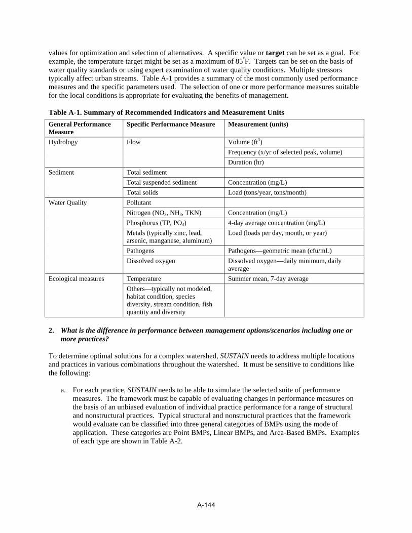
values for optimization and selection of alternatives. A specific value or target can be set as a goal. For exam ple, the temperature target might be set as a maximum of 85 °F. Targets can be set on the basis of water quality standards or using expert examination of water quality conditions. Multiple stressors typically affect urban streams. Table A-1 provides a summary of the most commonly used performance measures and the specific parameters used. The selection of one or more performance measures suitable for the local conditions is appropriate for evaluating the benefits of management.

Table A-1. Summary of Recommended Indicators and Measurement UnitsGeneral Measure

Performance Specific Performance Measure Measurement (units)

Hydrology Flow Volume (ft3) Frequency (x/yr of selected peak, volume) Duration (hr)

Sediment Total sediment Total suspended sediment Concentration (mg/L) Total solids Load (tons/year, tons/month)

Water Quality Pollutant Nitrogen (NO3, NH3, TKN) Concentration (mg/L) Phosphorus (TP, PO4) 4-day average concentration (mg/L) Metals (typically zinc, lead, arsenic, manganese, aluminum)

Load (loads per day, month, or year)

Pathogens Pathogens—geometric mean (cfu/mL) Dissolved oxygen

average Dissolved oxygen—daily minimum, daily

Ecological measures Temperature Summer mean, 7-day average Others—typically not modeled, habitat condition, species diversity, stream condition, fish quantity and diversity

2. What is the difference in performance between management options/scenarios including one or more practices?

To determine optimal solutions for a complex watershed, SUSTAIN needs to address multiple locations and practices in various combinations throughout the watershed. It must be sensitive to conditions like the following:

a. For each practice, SUSTAIN needs to be able to simulate the selected suite of performance measures. The framework must be capable of evaluating changes in performance measures on the basis of an unbiased evaluation of individual practice performance for a range of structural and nonstructural practices. Typical structural and nonstructural practices that the framework would evaluate can be classified into three general categories of BMPs using the mode of application. These categories are Point BMPs, Linear BMPs, and Area-Based BMPs. Examples of each type are shown in Table A-2.

A-144

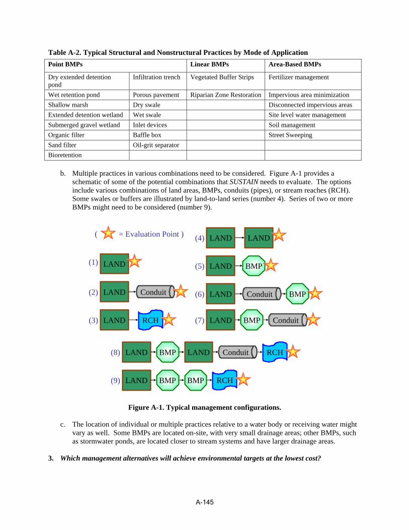
( = Evaluation Point ) (4)

(1) LAND (5) BMP

LAND LAND

LAND

(2) ConduitLAND (6)

(3) RCHLAND (7)

ConduitLAND BMP

ConduitLAND BMP

LAND LAND ConduitBMP RCH(8)

LAND BMP (9) BMP RCH

Table A-2. Typical Structural and Nonstructural Practices by Mode of Application Point BMPs Linear BMPs Area-Based BMPs

Dry extended detention pond

Infiltration trench Vegetated Buffer Strips Fertilizer management

Wet retention pond Porous pavement Riparian Zone Restoration Impervious area minimization Shallow marsh Dry swale Disconnected impervious areas Extended detention wetland Wet swale Site level water management Submerged gravel wetland Inlet devices Soil management Organic filter Baffle box Street Sweeping Sand filter Oil-grit separator Bioretention

b. Multiple practices in various combinations need to be considered. Figure A-1 provides a schematic of some of the potential combinations that SUSTAIN needs to evaluate. The options include various combinations of land areas, BMPs, conduits (pipes), or stream reaches (RCH ). Some swales or buffers are illustrated by land-to-land series (number 4). Series of two or mo re BMPs might need to be considered (number 9 ).

Figure A-1. Typical management configuratio ns.

c. The location of individual or multiple practices relative to a water body or receiving water might vary as well. Some BMPs are located on-site, with very small drainage areas; other BMPs, such as stormwater ponds, are located closer to stream systems and have larger drainage areas.

3. Which management alternatives will achieve environmental targets at the lowest co st?

A-145

The effectiveness of BMP options (sizes, locations) in achieving the desired water quality goal must be com pared based on costs. The scenarios can also be evaluated base d on the cost required to achieve the desired environmental condition. For each individual practice or combination of practices, the system will in lude a method for estimating the costs c of construction and O&M (Heaney et al. 2002).

A.2. Technical Requirements Specific technical requirements were defined for the identified needs. For example, consideration of the full set of indicators (hydrology, sediment, pollutants, and ecological impact) requires simulation of dynamic hydrology and time-varying loads of sediment and pollutan ts, and potentially other ecological indicators such as temperature or relationships to biological indic ators. Evaluating the implications of various configurations of management practices requires the ability to consider the performance of individual and multiple practices and the sensitivity of each of those practices to their relative location in the network. It is usually necessary to simulate longer time periods and storm sequences to demonstr ate response to a wide set of forcing conditions. The technical requirements for SUSTAIN are listed below.

• Simulate hydrologic response and a level of detail sufficient for analysis of a hydrograph (peak flow and volume)

• Simulate multiple pollutant types, including nutrients (nitrogen and phosphorus), pathoge ns (fecal coliform bacteria, Escherichia coli [E. coli]) and metals (e.g., zinc, aluminum)

• Simulate fate and transport of poll utants at a time step suitable for evaluating short-duration and long-duration impacts consisten t with evaluation of acute and chronic surface water criteria

• Simulate multiple size classes of sediment for input to management structures • Simulate other habitat stressors, such as temperature • Simulate in-stream dissolved oxygen based on inputs of biological oxygen demand, sediment

oxy gen demand, nutrient loads, and other environmental factors • Evaluate urban and mixed land uses, including pervious and impervious areas • Consider a full range of management practices at a similar level of spatial resolution and

technical detail • Consider distributed or small-scale upstream management practices, practices in series, and large r

downstream facilities • Link watershed management to downstream measures of environmental conditions (e.g.,

dissolved oxygen in a river, nutrient concentra tion in a lake or estuary) outside the immediate vicinity of a study area

Consequently, specific modeling procedures and algorithms were determined to fulfill the objectives of SUSTAIN. For example, simulation of hydrologic response requires that the model support the examination of rainfall/runoff processes at a level of detail sufficient to plot a time variable hydrograph and/or a pollutograph. Supporting model applications at multiple scales is essential for the SUSTAIN application. Scale may vary widely depending on the location and size of a watershed. The need to provide a modular modeling system and multiple scale applications govern the software and system designs.

A.2.1. Spatial Scale One dominant technical requirement of SUSTAIN is the ability to site management practices at multiple scales. The way that BMPs are placed at different spatial levels, i.e. on-site, sub-regional, and regional (Figure A-2), influences the overall cost-effectiveness of the stormwater controls system (Zhen 2002). In

A-146

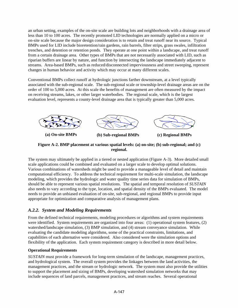
an urban setting, examples of the on-s ite scale are building lots and neighborho ods with a drainage area of less than 10 to 100 acres. The recently promoted LID technologies are normally applied on a micro or on-site scale because the major design consideration is to retain and treat runoff near its source. Typical BMPs used for LID include bioretent ion/rain gardens , rain barrels, filter strips, grass swales, infiltration trenches, and detention or rete ntion ponds. They oper ate at one point within a landscape, and treat runoff from a cer tain drain age area. Other typ es of BMPs that are not necessaril y associated with LID, such as riparian buffers are linear by nature, and function by intersecting the landscape immediately adjacent to streams. Area-based BMP s, s uch as r educed/disco nne cted imperviousness and street sweeping, represent changes in human behavior and activity which may occur at many different scale s.

Convent i onal BM Ps co lle c t r unoff at hy drologic junct i ons farther d ownstream , at a level typically associated with the sub-regional scale. The sub-regional scale or township-level drainage areas are on the order of 100 to 5,000 acres. At this sc a le the benefits of management are often measured by the impact on receiving streams, lakes, or other lar ger w a terbodies. The regional scale, whic h is the largestevaluation level, represents a county-level drai nage ar e a that i s typically greater than 5,000 acres.

(a) On-site BMPs (b) Su b-regional BMPs (c) Regional BMPs

Figure A-2. BMP p lacement a t various spatial levels: (a) on-site; (b) sub-regional; and (c) regio nal.

The system may ultimately be applied in a tiered or nested application (Figure A-3). More detailed small scale applicatio ns could b e co mb ined and evaluated on a large r scale to develop optimal solutions. Various com binations of w atersheds m ight be used to provide a manageable leve l of detail and ma intain com p utation al efficiency. To address the technical requirement for m ulti -scale si mulatio n, the l andscapemodeling, which provi des the hydrol ogic a nd water quality time series data for si mulatio n of BM Ps, should be able to represent various spatial resolu tions. The spatial and temporal resolution of SUSTAIN also needs to vary according to the ty pe, location, and spa tial density of the BM Ps evaluated. The m odelneeds to provide an unbiased evaluation of on-site, sub-regional, and regional BMPs to provide input appropriate for optimization and comparative analysis of management plans.

A.2.2. System and Modeling Requirements From the defined technical requirements, modeling procedures or algorithms and system requiremen ts were identified. Syste m re quirements are organized into four area s: (1) operational system fe atures, (2) watershed/landscape s imu latio n, (3) BMP simu lation, and (4) stream conveyance simul ation. While evaluating the candidate m odeling algorithm s, som e of the practical c onstraints, limitati ons, and capabilities of each alternative were considered. Also considered were the simul ation o ptions and flexibility of th e application. Each sy stem r equirem ent category i s de scribed in more de tail below.

Operational Requirements SUSTAIN must provide a framework for long-term sim ulation of the landscape, management practices, and hydrological system. The overall syste m provides the linkages between the land ac tivities, the management practices, and the stream o r hy drologic network. The sy stem must also provide the utilities to support the placement and sizing of BMPs, developi ng watershed simulation n etwork s that may include sequences of land parcels, mana gem ent pra ctic es, and stream reac hes. Several operatio nal

A-147

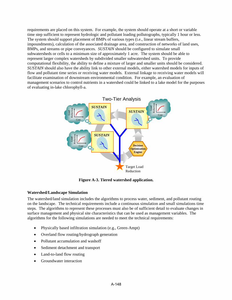
requirements are placed on this system. For example, the system should operate at a short or variable time step sufficient to represent hydrologic and pollutant loadin g pollutographs, typically 1 hour or less . The system should support placement of BMPs of various t ypes (i.e., linear stream buffers, impoundments ), calculation of the associated drainage area, an d construction o f netwo rks of land us es, BMPs, and streams or pipe conve y ances. SUSTAIN should be configured to si mulate small subwatersheds or cells to a minimum s ize of approx imately 1 acre. The system s hould be able to represent large r complex watersheds b y subdivided smaller su bwatershed units. To providecomputational flexibility, the abilit y to define a mixture of larger and smaller un its should be considered. SUSTAIN should also have the abil ity lin k to other external m odels, either watershed models for inputs of flow and pollutant time series or rec eiving water models. External linkage to receiving water models will facilitate examination of downstream environm ental condition. For example, an evaluation of managem ent scenarios to control nutrients in a watershed could be linked to a l ake model for the purposes of evaluating in-lake chlorophyll-a.

Two-Tie r Anal ysis

Load

Lo

ad

Red

u ctio

nR

educ

tion

SUSTAIN SUSTAIN Lo

ad

Red

uctio

n

Cost

Cost

SUSTAIN

Cost Decision Optimization

Engine

Targ Redu

et Load ction

Figure A-3. Tiered wat shed er application.

Watershed/Landscape Simulation The watershed/ land simu lation includes the algorithms to proce ss water, sedim ent, an d pollutant ro uting on the landscap e . The technical requirem ents include a conti nuous simulation and sm all simu lations tim esteps. The algorithms to represent these processes must also be of suffi cient detail to evaluate changes in surface management and physical site characteristics that can be used as management variables. The algorithms for the following simulations are needed to meet the technical requirem ents:

• Physically based infiltration simulation (e.g., Green-Am pt) • Overland flow routing/hydrograph generation • Pollutant accumulation and was hoff • Sediment detachment and transp ort • Land-to-land flow routing • Groundwater interaction

A-148

BMP Simulation A wide range of BMPs, both structural and nonstructu ral, needs to be evaluated by SUSTAIN. The simulation methods must provide an unbiased evaluation of the effectiveness of BMPs. Nonstructural management practices ca n include minimizing impervio us areas, augmenting soil infiltration capacity through lawn management, recycling o f roof runoff (e.g., usin g rain barrels), and disconnecting impervious surfaces (e.g., rain gutter outlets). Nonstruc tural management practices may also include source controls such as min imizing or reducing fertilize r and pesticide applications. N onstructural practices can be evaluated by adjusting imperviou s areas, changing pollutant acc umulation rates (e.g., changes in fertilizer application rates), or cha nging surface roughness characteristics (e.g., vegetative management). Nonstructural practices are area-based si nce the dominant manage ment is spatially distributed.

Structural practices involve the placement and construction of a facilit y that captures and manages runoff from a site. Structural practices are typically point-bas ed, since they are in a specific location and manage runoff captured from a defined drainage area. The typical practic es use various combinations of storage, infiltration, filtration, biological processes, and hydrologic separation to provide control of hydrology and remove or reduce sediment and pollutants. Table A-3 provides a summary of the dominant and secondary functional processes employed in various structural ma nagement practices. Some management practices employ additional processes, identifie d as optional on the table, depending on the specific design features and the site conditions. F or example, a sto rmwater detention facility might use infiltration as well as deposition/settling if the site h as permeable soils with suf ficient infiltration capacity. Table A-3 shows that many practices use similar proces ses to achieve flow, sediment, and water quality control. The table also identified the need for a management pra ctice modeling system that can simulate these key processes, including storage/detention, infiltration, filtration, biological uptake/conversion, and hydrodynamic separation. The technical requirement to simulate these processes supports the selection of the algorithms for simulation of BMPs.

The following specific capabilities are recommended:

• Process-based simulation of retention and detention types of management with, at a minimum, first order decay and settling

• Time series simulation of point-based structural management practices that considers runoff routing and hydrodynamic separation

• Area-based practices, including surface cover management, through the use of watershed/ landscape analysis

• Linear practices such as riparian buffers by routing surface and sub-surface runoff/pollutants from one land unit to the next

Stream Conveyance Simulation The stream routing and conveyance network component provides a linkage between subwatershed/landscape units, management practices, and other direct discharges within an urban watershed. The stream conveyance module is used to route runoff, sediment, and pollutants through a stream network, which is often present in an urban watershed. The rigor of simulation for the stream portion is related to the dominant processes present in urban streams. Key features include settling, resuspension, and decay (i.e., fecal coliform) and changes in the stream channel (i.e., stream bank erosion or degradation). Therefore, during conveyance in a stream, the module should consider settling, resuspension, and decay processes. Accounting for stream bank erosion should be considered as an option as well. Larger waterbodies, including rivers, lakes, and tidal waters might require more detailed simulation of chemical and biological processes. These systems can best be simulated through external

A-149

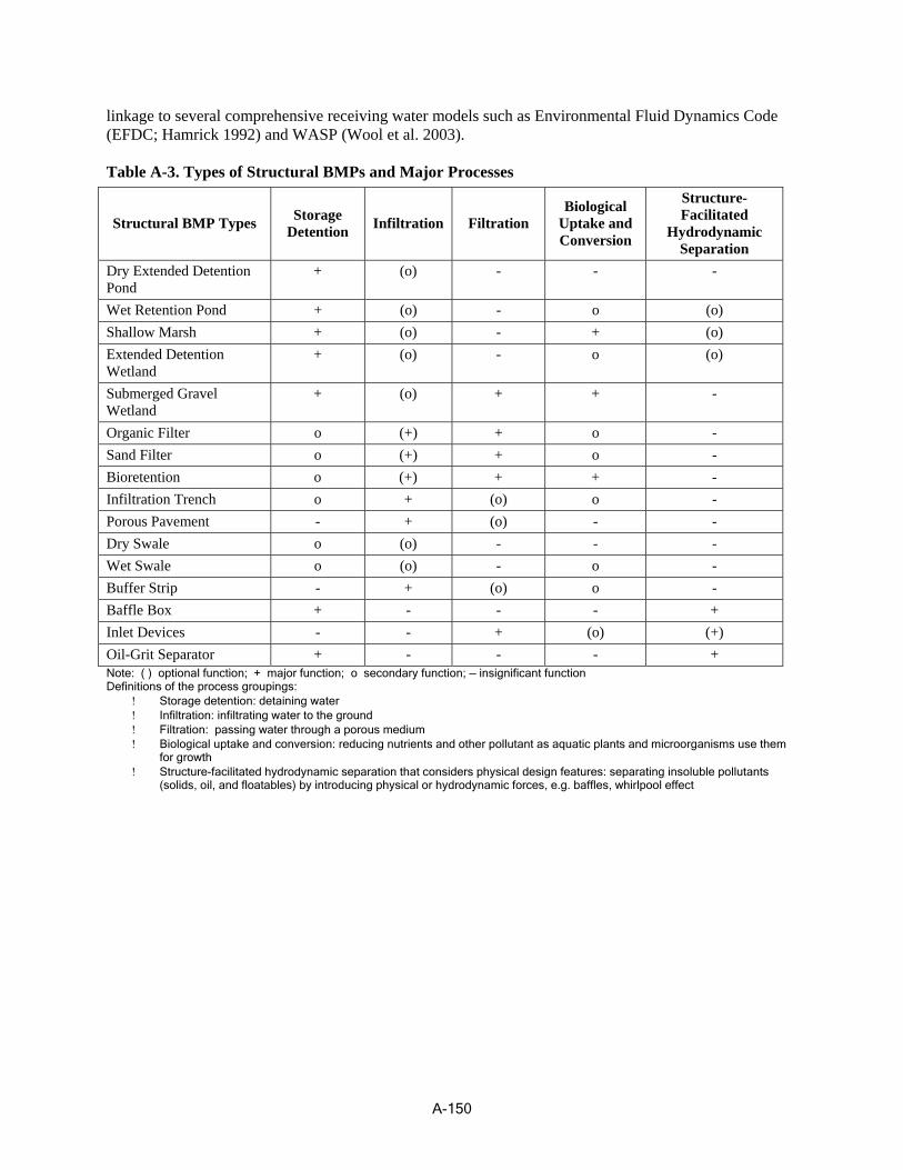
linkage to several comprehensive receiving water models such as Environmental Fluid Dy namics Code (EFDC; Hamrick 1992) and WASP (Wool et al. 2003).

Table A-3. Types of Structural BMPs and Major Processes

Str al B peuctur MP Ty s Stor Dete

age ntion Infiltrat ion trFil ation

ogical Uptake an C er

Biol

onv d

sion

u re-

o amic a

Str Facilitated

Hydr Sep

ctu

dyn ration

Dry ed on Pond

Extend Detenti + (o) - - -

Wet Retention ndPo + (o) - o (o) Shallow Mars h + (o) - + (o) Extende ete n Wetland

d D ntio + (o) - o (o)

Submerged Gravel Wetland

+ (o) + + -

Organic Filter o (+) + o -Sand Fi lter o (+) + o -Bioretention o (+) + + -Infi rltration T ench o + (o) o -Poro mus Pave ent - + (o) - -Dry Swale o (o) - - -Wet Swale o (o) - o -Buffer Strip - + (o) o -Baffle Box + - - - + Inlet Devices - - + (o) (+) Oil-Grit Separator + - - - + Note: ( ) optional function; + major function; o secondary function; — insignificant function Definitions of the process groupings:

! ra ion: detaining water Sto tentge de ! tra trating water to roundInfil infil tion: the g ! atFiltr ion: ing er throu porous medium watpass gh a ! Biological uptake and conversion: reducing nutrients and other pollutant as aquatic plants and mic s use them roorgani sm

for growth ! Structure-facilitated hy dyna separation that iders physical design features: separa nsoluble dro mic cons ting i llutants po

, oil, and flo by i ucing physical drodynamic fo , e. ffles, whirlp ffect les) ntrod or hy ool e (solids atab rces g. ba

A-150

B

Appendix B. Model Evaluation and Selection

B.1. Introduction This appendix provides a summary of the targeted evaluation and selection of public-domain software in accordance with the design requirements of SUSTAIN. Currently available models and modeling frameworks were identified and evaluated according to their technical capabilities and software system s. The review effort focused on identifying key models that addressed one or more of the needed algorithm s or analysis methods. The purpose of the review was to identify candidate models or portions of mode ls for integration or adaptation into SUSTAIN.

B.2. Overview of Available Models The review of available models followed a structured process based on the results of the technical needs analysis. Generally the review focused on publicly available models and modeling systems, although proprietary models that have been published and have relevant capabilities were included for comparative purposes. The following are some example considerations in the selection of available models for review:

• Is the model in the public domain, and how easily adaptable, current, and available is the source code for the model?

• Is the model well established with an extensive application history and record? • Is the model appropriate for small to mid-size urban watersheds? • How rigorous are its algorithms in simulating watershed processes? • Is the model relevant for pollutants present in urban areas? • Does the system include in terface capabilities or linka ges that could be relevant to the SUSTAIN

design?

The selection of models for review focused on identifying models t hat could have relevance to one or more areas of SUSTAIN. For this reason some models with specialized features that are not typically used in urban environm ents (e.g., WAMView [SWET 2002]) were included. The emphasis was on selection of models that are in the public dom ain or are available for distributio n without charge. Other proprietary models with lim ited information on model algorithms and documentation were exclu ded from the analysis (i.e., Mike-SHE, MOUSE [DHI Inc. Web site]). The set of models sele cted for review is listed in Table B-1 and profiles for each model are provided in Section B.3. A distinct set of evaluation factors was developed for watershed mo dels, BMP systems, and interface and s oftware platforms.

B-151

Table B-1. Available Models Reviewed Watershed Models BMP Models SWMM, HSPF, LSPC, WAMview, WARMF, SLAMM, P8 UCM, ANSWERS, CASC2D, KINEROS, WEPP, DR3M-QUAL, SWAT, AnnAGNPS, AGNPS, GWLF Systems: BASINS, EPA TMDL Toolbox

Prince George’s County BMP Module, P8 UCM, VFSMOD, MUSIC, DMSTA, SWMM, BMPAM Systems: LIFE

B.2.1. Watershed Model Evaluation Factors The following factors were identified for evaluation of available watershed models. The evaluation results are summarized in Table B-2. These factors are closely aligned with general modeling considerations and the four major categories of simulation needs (i.e., land, reach, conduit, and BMP).

• At what spatial scale (cell, field, catchment, subwatershed, or watershed) is the modeling application most suitable?

• At what time scale (continuous or event-based) is the simulation performed, and what is the minimum applicable computation time step?

• What land uses (urban and nonurban) can be simulated? Are point sources addressed? • How rigorous are its algorithms for hydrology simulation, how is the rainfall-runoff simulation

performed, and is groundwater interaction included? • How rigorous are its algorithms at water quality (pollutant loading) simulation? How does it

address sediment, nutrients, and other pollutant loading generation, transport, and transformation, if included?

In landscape or watershed models, an essential feature is how the area is segmented. For evaluation purposes segmentation was defined as four distinct options:

• Catchment (CM): Capable of simulating multiple watersheds and subwatersheds • Cell: Watershed area represented as a network of cells. Flow is routed from cell to cell • Field: Limited to a small single simulation unit, typically a field or monitoring plot • Watershed (Wsh): Limited to single watershed for each model simulation

B.2.2. BMP Technical Evaluation Factors The following factors were considered in BMP model evaluation as summarized in Table B-3.

• What types of BMPs can be addressed? • What pollutant removal processes and mechanisms are simulated? • What algorithms are applied for flow routing and pollutant removal process simulation? • What water quality constituents can be simulated?

B.2.3. Model Interface Evaluation Factors The model interface features of the models were evaluated, using the following factors:

• What GIS features, if any, are incorporated?

B-152

• How is the subwatershed/channel network represented? • Data management utilities • Model code • Interface code

Table B-4 and Table B-5 contain model interface evaluations for watershed models.

B.3. Evaluation and Review of Available Models This section provides an evaluation and review of available models. The models reviewed are organized into three groups—landscape models, BMP models, and comprehensive modeling systems. Within each group, the models are sequenced based on their expected relevance to urban management analysis. Regardless of their position in the sequence, all models reviewed might have specific features that could prove useful for the development of SUSTAIN. A narrative discussion is provided below for each mode l, including key features, capabilities, special techniques, and software capabilities. The narrative description supports earlier summary tables (Table B-2 to Table B-5). Section B.4 provides further discussion of the strengths and weaknesses of the reviewed models and identifies the models for integration into the SUSTAIN design.

B.3.1. Landscape Model Reviews Landscape models are models that simulate land-based hydrology and water quality, and provide sediment and pollutant loading estimates. Many of these models also incorporate some of the features of BMP models (i.e., simulation of various management practices) and stream conveyance systems. The following landscape models were reviewed for potential integration of components and interface with SUSTAIN.

SWMM The Stormwater Management Model (S WMM) is a dynamic rainfall-runoff simulation model developed by EPA and primarily applied to urban areas, for single-event or long-term (continuous) simulation using various time steps (Huber and Dickinson 1988). It was developed for the analysis of surface runoff and flow routing through complex urban sewer systems. The last official version was 4.4h. SWMM5 is a completely revised and updated release of SWMM. However, SWMM5 will continue to be expanded with new functions, particularly a quality routine.

In SWMM, flow routing is performed for surface and subsurface conveyance and groundwater systems, including the options of nonlinear reservoir channel routing and fully dynamic hydraulic flow routing. By choosing the fully dynamic hydraulic flow routing option, SWMM can simulate backwater, surcharging, pressure flow, and looped connections. SWMM has a variety of options for quality simulation, including the traditional buildup and washoff formulation, as well as rating curves and regression techniques. The Universal Soil Loss Equation (USLE) is included to simulate soil erosion. SWMM incorporates first-order decay and particle-settling mechanisms in pollutant transport simulations, including the option of a simple scour-deposition routine in conduits. Storage, treatment, and other BMP s can also be simulated. A more detailed description of its BMP simulation capabilities is provided in the next section.

B-153

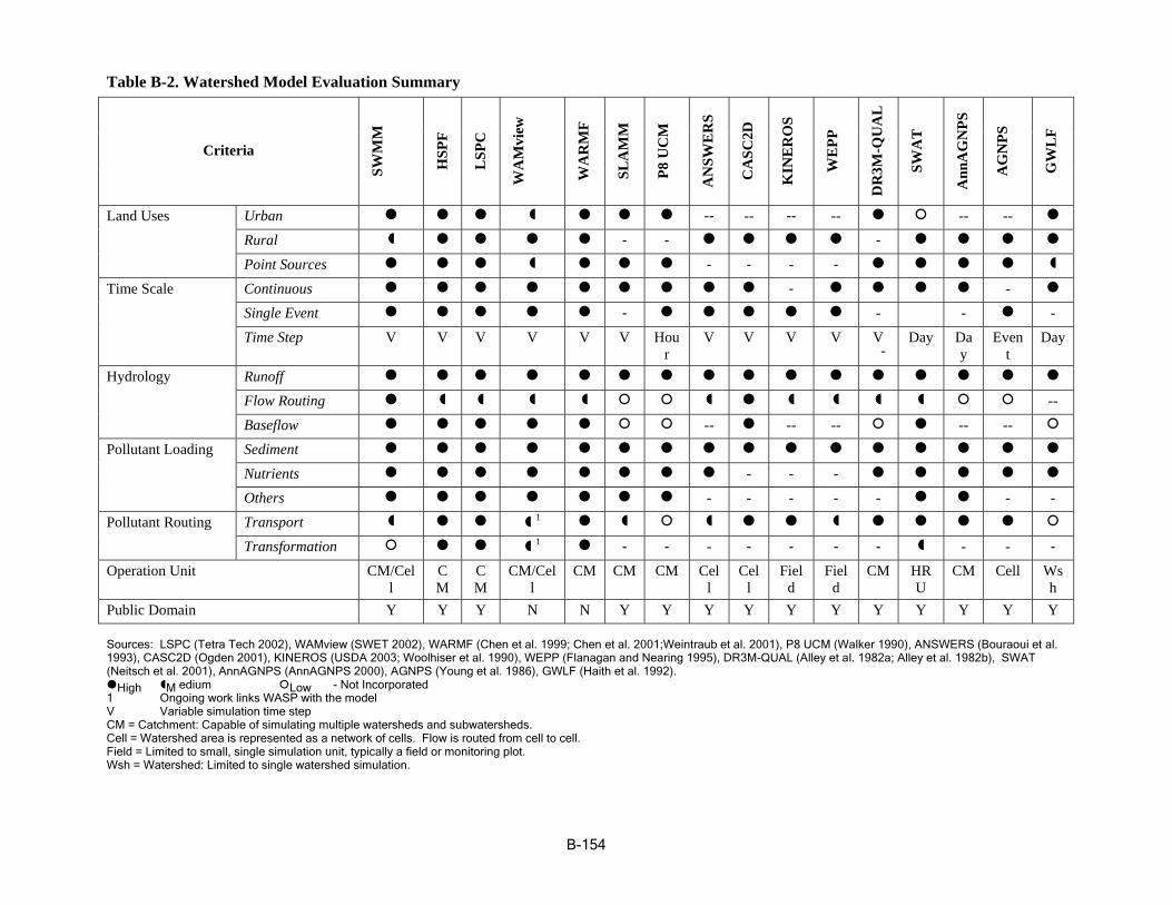
B-154

Table B-2. Watershed Model Evaluation Summary

Criteria

SWM

M

HSP

F

LSP

C

WA

Mvi

ew

WA

RM

F

SLA

MM

P8 U

CM

AN

SWE

RS

CA

SC2D

KIN

ER

OS

WE

PP

DR

3M-Q

UA

L

SWA

T

Ann

AG

NPS

AG

NPS

GW

LF

Land Uses Urban z z z � z z z -- -- -- -- z | -- -- z

Rural � z z z z - - z z z z - z z z z

Point Sources z z z � z z z - - - - z z z z �

Time Scale Continuous z z z z z z z z z - z z z z - z

Single Event z z z z z - z z z z z -

-

- z -iT me Step V V V V V V Ho

r u V V V V V Day Da

y Even

t ayD

Hydrology Runoff z z z z z z z z z z z z z z z z

Flow Routing z � � � � | | � z � � � � | | --Baseflow z z z z z | | -- z -- -- | z -- -- |

Pollutant Loading Sediment z z z z z z z z z z z z z z z z

Nutrients z z z z z z z z - - - z z z z z

Others z z z z z z z - - - - - z z - -Pollutant Routing Transport � z z � 1 z � | � z z � z z z z |

Transformation | z z � 1 z - - - - - - - � - - -Operation Unit CM/Cel

l C M

C M

CM/Cel l

CM CM CM Cel l

Cel l

Fiel d

Fiel d

CM HR U

CM Cell s h

W

Public Domain Y Y Y N N Y Y Y Y Y Y Y Y Y Y Y

Sources: LSPC (Tetr a Tec h 2002), WAMview (SWET 2002), WARMF (Chen et al. 1999 ; Chen e t al. 2001;Weintraub et al. 2001), P8 UCM (Walker 1 990), ANSWERS (Bouraoui et a l.

1993), CASC 2D (Ogd en 2001), KINEROS (USDA 2003; Woolhiser et al. 1990), WEPP ( Flanagan and Nearin g 1995), DR3M-QUAL (Alley et al. 1982 a; All ey et al. 1982b), SWAT

(Neitsch et al . 2001), AnnAGNPS (AnnAGNPS 2000), AGNPS (Young et al. 1986), GWL F (Haith et al. 1992).

zHigh �M edium |Low - Not Incorporated

1 Ongoing w ork lin ks WASP with the model

V Variable si mulati on time step

CM = Catchm ent: Ca pable of sim ulating multiple watersheds and subwatersheds.

Cell = Water shed area is re pres ented as a network of cells. Flow is routed from cell to cell.

Field = Limite d to sma ll, sin gle simulation unit, typically a field or monitoring plot.

Wsh = Watershed: Limited to single wat ershed simulation.

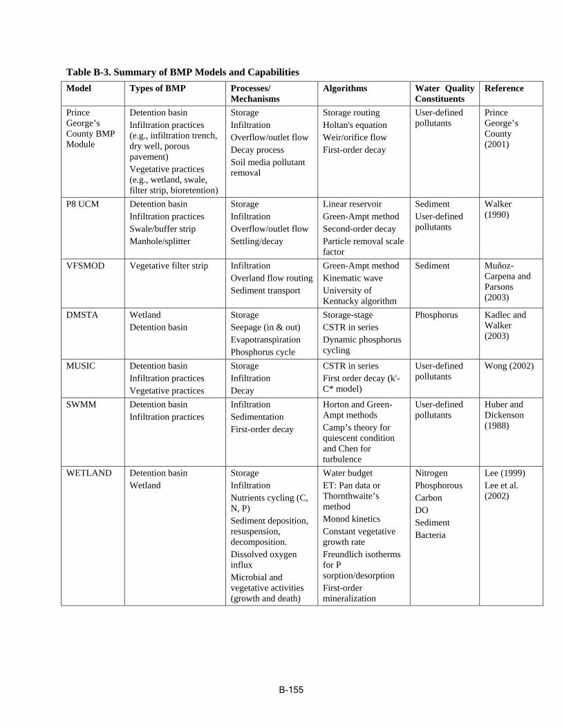
Table B-3. Summary of BMP Models and Capabilities Model Types of BMP Processes/

Mechanisms Algorithms Water Quality

Constituents Reference

Prince Detention basin Storage Storage routing User-defined Prince George’s Infiltration practices Infiltration Holtan's equation pollutants George’s County BMP Module

(e.g., infiltration trench, dry well, porous pavement) Vegetative practices (e.g., wetland, swale, filter strip, bioretention)

Overflow/outlet flow Decay process Soil media pollutant removal

Weir/orifice flow First-order decay

Co (2

unty 001)

P8 UCM Detention basin Infiltration practices Swale/buffer strip Manhole/splitter

Storage Infiltration Overflow/outlet flow Settling/decay

Linear reservoir Green-Ampt method Second-order decay Particle removal scale factor

Sediment User-defined pollutants

Walke (

r 1990)

VFSMOD Vegetative filter strip Infiltration

Sediment transport Overland flow routing

Green-Ampt method

University of Kentucky algorithm

Kinematic wave Sediment Muñoz-

Carpena and Parsons (2003)

DMSTA Wetland Detention basin

Storage Seepage (in & out) Evapotranspiration Phosphorus cycle

Storage-stage CSTR in series Dynamic phosphorus cycling

Phosphorus Kadlec and Walker (2003)

MUSIC Detention basin Infiltration practices Vegetative practices

Storage Infiltration Decay

CSTR in series First order decay (k'­C* model)

User-defined pollutants

Wong (2002)

SWMM Detention basin Infiltration practices

Infil Sedimentation First-order decay

tration Ampt methods Camp’s theory for quiescent condition

Horton and Green­

bulence and Chen for tur

pollutants User-defined

D (1

Huber and ickenson 988)

WETLAND Detention basin Wetland

Storage Infiltration

vegetative activities (growth and death)

Nutrients cycling (C, N, P) Sediment deposition, resuspension, decomposition. Dissolved oxygen influx Microbial and

Water budget ET: Pan data or

First-order mineralization

Thornthwaite’s method Monod kinetics Constant vegetative growth rate Freundlich isotherms for P sorption/desorption

Nitrogen Phosphorous Carbon DO Sediment Bacteria

Lee (1999) Lee et al.

02) (20

B-155

Table B-3. (Continued) Model Types of

BMP Processes/ Mechanisms Algorithms Water Quality

Constituents Reference

VAFSWM Detention basin Wetland

Storage Infiltration Particle settling Adsorption to plant and substrate Vegetative uptake

Water budget ET: user specified rate CSTR in series First-order kinetics (adsorption, plant uptake)

User-defined pollutants Sediment

Yu, and (199

Fitch Earles 8)

REMM Vegetative buffer strip

Infiltration Evaportransporation Surface and subsurface flow routing Nutrients cycling (C, N, P)

Sediment transport Erosion

Green-Ampt equation ET: modified Penman Monteith equation, and Darcy Buckingham equation Storage routing Darcy’s equation Nutrient cycling: Century

Erosion: USLE Sediment transport: Einstein and Bagnold equations

Model Nitrification: First-order Weir/orifice flow

Sediment Nutrients (C, N, P)

USDA AR (19

SEWRL, -

S 99)

SWMM has been applied to address various urban water quantity and quality problems in many locati ons in the United States and other countries (Donigian and Huber 1991; Huber 1992). In addition to its use i n developing comprehensive watershed-scale planning, typical uses of SWMM include predicting CSOs, assessing the effectiveness of BMPs, and providing time series input to dynamic receiving water quality models (Donigian and Huber 1991.)

HSPF Hydrological Simulation Program–FORTRAN (HSPF) is a comprehensive package developed by EPA for simulation of watershed hydrology and water quality for both conventional and toxic organic pollutants (Bicknell et al. 1997). This model can simulate the hydrologic and associated water quality processes on pervious and impervious land surfaces and in streams and well-mixed impoundments. HSPF incorporates the Agricultural Runoff Management (ARM) model and Nonpoint Source Runoff (NPS) model into a wat ershed analysis framework that includes fate and transport in one-dimensional stream channels. It allows the integrated simulation of land and soil contaminant runoff processes with in-stream hydraulic and sediment-chemical interactions. The result of this simulation is a time history of the runoff flow rate, sediment load, and nutrient and pesticide concentrations, along with a time history of water quantity and quality at any p oint in a watershed.

HSPF simulates three sediment types (sand, silt, and clay) in addition to a single organic chemical a nd transformation products of that chemical. Further, the in-stream model assumes that the receiving waterbody is well mixed with width and depth and is t hus limited to well-mixed rivers and reservoirs. The transformation and reaction processes include hydrolysis, oxidation, photolysis, biodegradation, volatilization, and sorption. Sorption is modeled as a first-order kinetic process in which the user must specify an adsorption and desorp ion rate and an equilibrium partition coefficient for each of the three solids types. t Resuspension and settling of silts and clays (cohesive solids) are defined in terms of shear stress at the sediment water interface. The model computes the capacity of the system to transport sand at a particular flow. Settling and/or scouring are defined by the difference between the sediment load in suspension and the transport capacity.

B-156

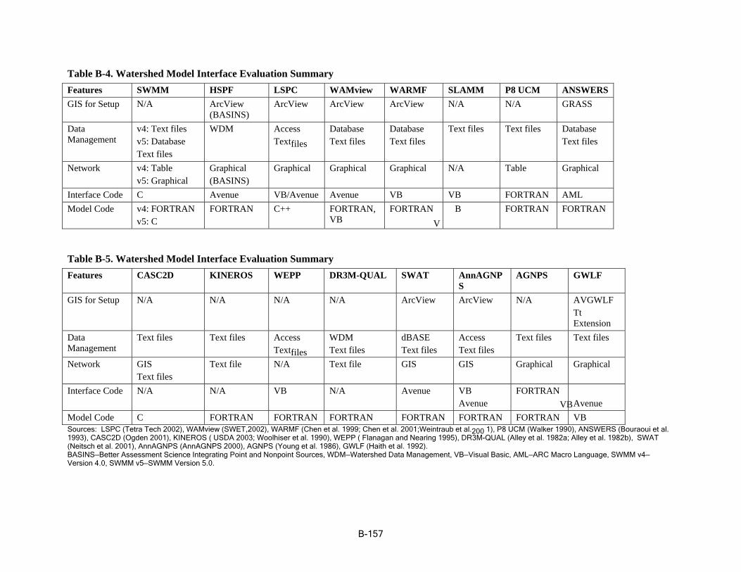
B-157

Table B-4. Watershed Model Interface E valuation Summary Features SWMM SPFH LSPC WAMview WARMF LAS MM UP8 CM ANSWERS GIS for Setup N/A A

(B rcView ASINS)

ArcView ArcView ArcView /N A AN/ GRASS

Data v4: Text files DMW Access Database Database Text files tTex files Database Management v5: Data base Text files Text files Text files Text files

Text files Network v4: Tabl

v5: Grap e hical

raphical ASINS)

G (B

Grap hical Graphical Graphical N/A leTab Graphical

Interface Code C Avenue VB/Avenue Avenue VB VB R NFO TRA AML Model Code v4: FOR

v5: C TRA N ORTRANF C++ FORTRAN,

VB FORTRAN

VB R NFO TRA FORTRAN

Table B-5. Watershed Model Inte rface Eva luation Summary Features CASC2 D INEK ROS WEPP DR3M-QUAL SWAT GNP AnnA

S AGNPS GWLF

GIS for Setup N/A N/A N/A N/A ArcView wArcVie N/A AVGWLF Tt Extension

Data Text files ext filesT Access WDM dBASE Access Text files Text files Management Text files Text files Text files Te esxt fil Network GIS

Text files ext file T N/A Text file GIS GIS Graphical Graphical

Interface Code N/A N/A VB N/A Avenue V Av

B enue

FORTRAN VB Avenue

Model Code C FORTRAN FORTRAN FORTRAN NFORTRA FORTRAN FORTRAN VB Sources: LSPC (Tetra Tech 20 02), WA Mview (SWET,2002), WAR MF (Chen et al. 1999; Chen et al. 2001;Weintraub et al. 200 1), P8 UCM (Walker 1 990), ANSWERS (Bouraoui et al.

1993), CASC2D (Ogden 2001) , KINER OS ( U SDA 2003; Woolhiser et al. 1990), WEPP ( Flanagan and Nearing 1995), D R3M-QUAL (Alley et al. 198 2a; Alley et al. 1982b), SWAT

(Neitsch et al. 2001), AnnAGN PS (AnnAGNPS 2000), AGNPS (You ng et al. 1986), GWLF (Haith et al. 1992).

BASINS—Better Assessment S cience Integrating Point and Nonpoin t Sources, WDM—Watershed Data Managem ent, VB—Visual Basic, AML—ARC Ma cro Language, SWMM v4—

Version 4.0, SWMM v5—SWM M Version 5.0.

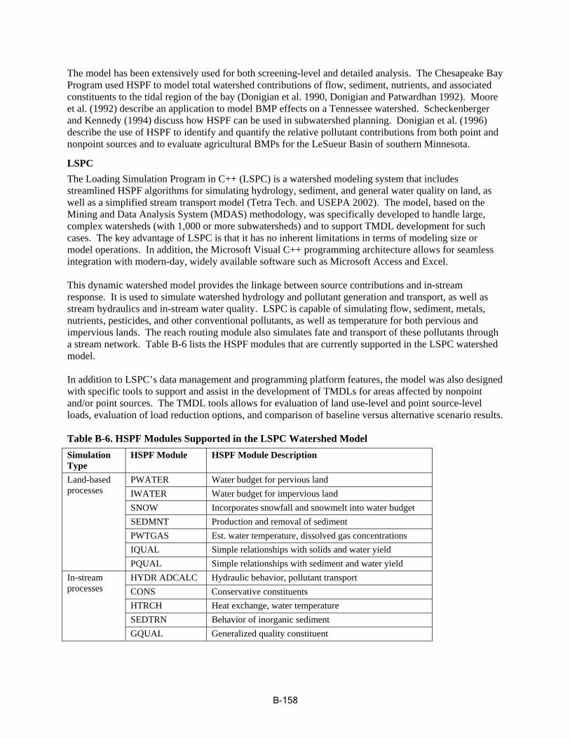
The model has been extensively used for both screening-level and detailed analysis. The Chesapeake Bay Program used HSPF to model total watershed contributions of flow, sediment, nutrients, and associated constituents to the tidal region of the bay (Donigian et al. 1990, Donigian and Patwardhan 1992). Moore et al. (1992) describe an application to model BMP effects on a Tennessee wate rshed. Scheckenberger and Kennedy (1994) discuss how HSPF can be used in subwatershed planning. Donigian et al. (1996) describe the use of HSPF to identify and quantify the relative pollutant co ntributions from both point and nonpoint sources and to evaluate agricultural BMPs for the LeSueur Basin of southern Minnesota.

LSPC The Loading Simulation Program in C++ (LSPC) is a watershed modeling system that includes streamlined HSPF algorithms for simulating hydrology, sediment, and general water quality on land, as well as a simplified stream transport model (Tetra Tech. and USEPA 2002). The mode l, based on the Mining and Data Analysis System (MDAS) methodology, was specifically developed to handle large, complex watersheds (with 1,000 or more subwatersheds) and to support TMDL development for such cases. The key advantage of LSPC is that it has no inherent limitations in terms of modeling size or model operations. In addition, the Microsoft Visual C++ programming architecture allows for seamless integration with modern-day, widely avail able software such as Microsoft Access and Excel.

This dynamic watershed model provides the linkage between source contributions and in-stream response. It is used to simulate watershed hydrology and pollutant generation and transport, as well a s stream hydraulics and in-stream water quality. LSPC is capable of simulating flow, sediment, metals, nutrients, pesticides, and other conventional pollutants, as well as temperature for both pervious and impervious lands. The reach routing module also simulates fate and transport of these pollutants through a stream network. Table B-6 lists the HSPF modules that are currently supported in the LSPC watershed model.

In addition to LSPC’s data management and programming platform features, the model was also des igned with specific tools to support and assist in the development of TMDLs for areas affected by nonpoint and/or point sources. The TMDL tools allows for evaluation of land use-level and point source-level loads, evaluation of load reduction options, and compariso n of baseline versus alternative scenario results.

Table B-6. HSPF Modules Supported in the LSPC Watershed Model Simulation Type

HSPF Module HSPF Module Description

Land-based PWATER Water budget for pervious land processes IWATER Water budget for impervious land

SNOW Incorporates snowfall and snowmelt into water budget SEDMNT Production and removal of sediment PWTGAS Est. water temperature, dissolved gas concentrations IQUAL Simple relationships with solids and water yield PQUAL Simple relationships with sediment and water yield

In-stream HYDR ADCALC Hydraulic behavior, pollutant transport processes CONS Conservative constituents

HTRCH Heat exchange, water temperature SEDTRN Behavior of inorganic sediment GQUAL Generalized quality constituent

B-158

WAMView Watershed Assessment Model (WAM) is a GIS-based model that allows engineers and land use planner s to interactively simulate a nd assess the environmental effects of various land use changes and associated land use practices (SWET 2002). WAM was originally developed with an Arc/Info interface for the entire Suwannee River Water Management District (SRWMD; 19,400 km2 of northern Florida) and h as since been customized for St. Johns River Water Management District (SJRWMD) in northeast Florida to accommodate its special regional and geological characteristics. The SJRWMD version includes an ArcView interface, and thus it is called WAMView. WAMView provides hourly time series of flow, TSS, and nutrients for all the contributing watersheds. The simulated hydrologic parameters include source cell surface and groundwater flow, and stream reach d aily flow; simulated water quality parameters are suspended solids, sediment N, sediment P, soluble N, soluble P, BOD, bacteria, and toxics. The model provides water quality daily outputs at source cells, subbasins, and stream reaches. An effort is under way to link WAMView to the WASP model.

The water quality assessments are accomplished using two methods. The first method provides spatial assessment using impact indices, and the second uses detailed hydrologic and water quality transport modeling. The method used depends on the watershed assessment parameter of interest. The indexing approach is used for parameters that are hard to quantify and that are also directly associated with pollutant transport, while the modeling approach add resses the major pollutants of sediment and nutrients. Both approaches provide outputs at the source cell, sub-basin, and basin outlet levels. Both approaches use the watershed characteristic data from existing GIS coverage to determine the appropriate inp ut data (indices for index approach and model parameter sets for the modeling approach). These data are used to calculate the combined impact of all watershed characteristics for a given grid cell. Once the combined impact at each unique cell within a watershed is determined, the cumulative impact for the entire watershed is determined by first attenuating the constituent to the subbasin outlets and then calculating a n area-weighted ranking/index at the attenuated load generated at each cell. Constituents are attenuated based on the flow distances (overland flow route to nearest waterbody, through wetlands or depressions, and within streams to the subbasin outlet), flow rates in each related flow path, and types of wetlands or depression encountered. The contaminant transport modeling is accomplished by first simulating all the unique grid cell combinations of land use, soils, and rain zone by using a unique cell model that contains several source cell models, including GLEAMS (Knisel 1993), EAAMOD (SWET 1999), a wetland module, and an urban module. The unique cell model, also called the BUCSHELL (Basin Unique Cell Shell Program) model, operates on square grid cells with a typical size of 1 hectare (100 m x 100 m) . The cell model simulates the daily flow and constituents from each unique cell within the watershed u sing one of the four submodels unique to WAMView, e.g., GLEAMS, EAAMOD, URBAN, and WETLAND, depending on land uses and soil. The time series outputs for each grid cell are routed and attenuated to the nearest stream and then routed through the stream using WAMView’s BLASROUTE (Basin Land and Stream Routing) module. The BLASROUTE module predicts flow, stage, and water quality. It routes through a stream network with attenuation, also routes through depression and wetlands. The model uses linear reservoir flow routing, and applies attenuation based on flow rate, characteristics of flow path, and flow distance. It also allows outlet stage and concentration definition with backflow.

WAMView is limited for SUSTAIN because of its development and application emphasis on rural areas. However, the cell-based representation and model configuration process provide potential benefits for assessing the localized loading and spatial implications in the placement of BMPs.

WARMF WARMF (Watershed Analysis Risk Management Framework) was developed by Systech Engineering, Inc., as a decision support system for calculating TMDLs (Chen 1999). The GIS map-based tool contains five interconnected modules: Engineering, Data, Knowledge, TMDL, and Consensus. In WARMF, a

B-159

wat hers ed is divided into a network of land catchments, stream segments, and stratified lakes. The engineering module is a dynamic watershed simulation model that calculates daily runoff, nonpoint source loads, groundwater flow, and hydrology and water quality of river segments and stratified reservoirs. The data module contains meteorological, air quality, point source, reservoir release, and f low diversion data. The nonpoint source loads are routed together with point source loads to predict water quality in rivers and lakes. The simulation models embedded in the WARMF engineering module were adapted from well-established simulation codes. The main computing engine was taken from the Integrated Lake-Watershed Acidification Study (ILWAS) model. The ILWAS model divides a watershed into land catchments, stream segments, and lake layers. Land catchments are further divided into canopy and soil layers. These watershed compartments are connected to form a network for hydrologic and water quality simulations.

The hydrologic model simulates the processes of canopy interception, snowpack accumulation and snowmelt, infiltration through soil layers, evapotranspiration from soil, exfiltration of groundwater to stream segments, kinematic wave routing of stream flows, and flow routing of reservoirs. Such detailed simulations track the flow paths of precipitation from canopy through soil layers and streams to lakes. Along each flow path, the chemistry module performs mass balance and chemical equilibrium calculations to account for the process es of dry deposition to the canopy, nitrification of ammonia on the canopy, ion leaching from sap to the canopy surface, washoff by through-fall, ion leaching by snowmelt, and the soil processes, e.g., litter fall, litter breakdown, litter decay, nitrification, denitrification, cation exchange, anion adsorption, weathering, and nutrient uptake.

The algorithms of WARMF were derived from many available codes. Algorithms for snow hydrology, groundwater hydrology, river hydrology, lake dynamics, and mass balance for acid base chemistry were based on the ILWAS model. Algorithms for erosion, deposition, resuspension, and transport of sediment were adapted and modified from ANSWERS. The pollutant accumulation on land surface was modified from SWMM. Instead of using export coefficients, an algorithm for mixing and washoff was used to simulate the processes that generate nonpoint source loading. The first-order decay of coliforms and BOD and its impact on dissolved oxygen follow the techniques used in traditional water quality models. The sediment adsorption-desorption of pesticides and phosphorus and the kinetics of nutrients and algal dynamics were adapted from WASP5.

WARMF provides step-by-step roadmaps for calculating TMDLs and for building consensus. WARMF also offers GIS-generated maps, tables, and graphing capabilities. In addition, the costs/benefits of pollutant trading, stakeholders, alternative ranking, and the nominal scores of rankings are calculated at the watershed scale. These tools can be used for management analysis at the watershed scale. Support for site-scale, land-use-specific, and subwatershed-level analyses is limited.

The major limitation of WARMF is that it is not a public domain model. WARMF is also oriented to rural land areas. The management and alternatives analysis is limited to watersheds, and simulation of multiple levels of controls by subwatershed/land use requires repeated simulation. The strength of WARMF is detailed representation of chemical processes, especially with respect to metals and pH.

SLAMM The Source Loading and Management Model (SLAMM) was originally developed to better understand the relationships between sources of urban pollutants and runoff quality (Pitt 1993). SLAMM is strongly based on actual field observations, with minimal reliance on pure theoretical processes that have not been adequately documented or confirmed in the field. It has been continually expanded since the late 1970s and now includes a wide variety of source area and outfall control practices (infiltration practices, wet detention ponds, porous pavement, street cleaning, catch basin cleaning, and grass swales). Beginning with version 5, SLAMM is Windows-based and thus is called WinSLAMM.

B-160

The model performs continuous mass balances for particulates and dissolved pollutants and for runoff volumes. Runoff is calculated by a method developed by Pitt (1987) for small-storm hydrology. Runoff is based on rainfall minus initial abstraction, and infiltration is calculated for both impervious and pervious areas. Triangular hydrographs, parameterized by a statistical approach, are used to simulate flow. Exponential buildup and rain washoff, as well as wind removal functions, are used in computing runoff pollutant loadings. Water and sediment from various source areas are tracked as they are rou ted through treatment devices. SLAMM is mostly used as a planning tool to better understand sources of urban runoff pollutants and the effectiveness of their control.

SLAMM is capable of considering many stormwater controls that affect source areas, drainage systems, and outfalls, for a long series of rainfall events. The program considers how particulates filter or settle out in control devices. Particulate removal is calculated based on the structural design characteristic s. Storage and overflow of devices are also considered. At the outfall locations, the characteristics of the source areas are used to determine pollutant loads in solid and dissolved phases. Another ability of SLAMM is to accurately describe a drainage area in sufficient detail for water quality investigations, but without requiring a great deal of superfluous information that field studies have shown to be of little value in accurately predicting discharge results. SLAMM also applies stochastic analysis procedures to more accurately represent actual uncertainty in model input parameters to better predict the actual range of outfall conditions (especially pollutant concentrations). Like all stormwater models, SLAMM needs to be accurately calibrated and then tested (verified) as part of any local stormwater management effort. The major limitation of SLAMM is that it is strongly based on a statistical approach that uses the current available field observations; therefore, it is not a process-based model. Some of the key features of the model have potential for incorporation into SUSTAIN. For instance, the algorithms and data used for addressing source control could be applied to SUSTAIN.

ANSWERS The Areal Nonpoint Source Watershed Environment Response Simulation (ANSWERS) model is a comprehensive model developed to evaluate the effects of land use, management schemes, and conservation practices or structures on the quantity and quality of water from agricultural or rural watersheds (Beasley 1986). It was among the first generation of distributed watershed models, which allow for a better analysis of spatial as well as temporal variabilities of pollutant sources and loads. It was initially developed on a storm event basis to enhance the physical description of erosion and sediment transport processes in agricultural watersheds. Data preparation for ANSWERS is rather complex, especially when watersheds are large. The output routines, however, are quite flexible and results are available in several tabular and graphical forms. The program has been used to evaluate management practices for agricultural watersheds and construction sites primarily in Indiana. It has been combined with extensive monitoring programs to evaluate the relative importance of point and nonpoint source contributions to Saginaw Bay in Michigan. This application involved the computation of unit area loadings under different land use scenarios for evaluation of the tradeoffs between load allocations (LAs) and wasteload allocations (WLAs). Recent model revisions include improvements to the nutrient transport and transformation subroutines (Dillaha et al. 1988). Bouraoui et al. (1993) describe the development of a continuous simulation version of the model.

The main limitation of ANSWERS is its emphasis on erosion and sediment transport in rural areas, w hich are not tested for primarily urban areas.

CASC2D The Cascade 2 Dimensional (CASC2D) sediment model is a fully unsteady, physically based, distributed-parameter, square-grid, two-dimensional, infiltration-excess (Hortonian) hydrologic model for simulating the response of a watershed subject to rainfall (Ogden 2001). Major processes simulated include

B-161

continuous soil-moisture accounting, rainfall interception, infiltration, surface and channel runoff routing , soil erosion, and sediment transport. Raster (square grid) is the computational unit. CAS2D allows the user to select a grid size (typically 30–200 m) that appropriately describes the spatial variability in all watershed characteristics. CASC2D is physically based and solves the equations of conservation of m ass and energy to determine the timing and path of runoff in the watershed. CAS2D applies Green and Ampt with or without a redistribution method for infiltration simulation; an explicit finite-difference, two-dimensional, diffusive-wave method for overland flow routing; and options of explicit one-dimensional, diffusive-wave or implicit dynamic-wave channel routing. The empirical Kilinc and Richardson (1973) soil erosion model as modified by Julien (1995) is applied in CASC2D to determine the sediment transport from one overland flow grid cell to the next. CASC2D employs Yangs’ (1973) me thod to routing sand-size sediment in stream channels. Silt and clay size sediment are assumed to be transported with flow; deposition or erosion of silt and clay within the channels is neglected (Ogden 1998). The physically based distributed model is superior in simulation of runoff process at small scales within the watershed. As a spatially distributed model, CASC2D offers the capability of determining the value o f any hydrologic variable at any grid point in the watershed at the expense of requiring significantly more input than traditional approaches. CASC2D can accept spatially varied hydrologic parameter input or rainfall input; however, because of the extensive data amounts required, data uncertainty may result in a non-unique calibration.

CASC2D development was initiated in 1989 at the Center for Excellence in Geosciences at Colorado State University funded by the United States Army Research Office (ARO). The original version of CASC2D has been significantly enhanced under funding from ARO and the U.S. Army Corps of Engineers Waterways Experiment Station (USACEWES). USACEWES has selected CASC2D as its premier two-dimensional surface water hydrologic model. CASC2D is also one of the surface-wate r hydrologic models supported by the Watershed Modeling System (WMS), developed at Brigham Young University. The GRASS GIS developed by the U.S. Army Constru ction Engineering Research Laboratories can be used in the preparation of CASC2D data sets.

itThe lim ations of CASC2D are as follows:

• CASC2D is a fully distributed, physically based, state-of-the-art hydrologic model, but with the exception of sediment, it does not have an integrated water quality component

• Because the program uses a distributed scheme and physically based algorithms, application requires extensive input data preparation and calibration

KINEROS The Kinematic Runoff and Erosion (KINEROS) model is an event-oriented, physically based model that describes the processes of interception, infiltration, surface runoff, and erosion from small agricultural and urban watersheds (USDA 2003). The model represents a watershed by a sequence of planes and channels and solves the partial differential equations describing overland flow, channel flow, erosion, and sediment transport by using finite-difference techniques. The spatial variations of rainfall, infiltration, runoff, and erosion parameters can be accommodated. KINEROS can be used to determine the effects of various artificial features, such as urban developments, small detention reservoirs, or lined channels on flood hydrographs and sediment yield. This model is suitable for small agricultural and disturbed urban watersheds.

The following are the limitations of KINEROS:

• It is an event-based model • It is primarily designed for small agricultural and disturbed urban areas

B-162

• It simulates only sediment

WEPP Developed by the U.S. Department of Agriculture’s (USDA) Agricultural Research Service (ARS), the Water Erosion Prediction Project (WEPP) model is a distributed-parameter, continuous-simulation mode l developed to provide a new generation of soil erosion prediction technology (USDA NSERL 1995). The model requires inputs for rainfall amounts and intensity; soil textural qualities; plant growth parameters ; residue decomposition parameters; effects of tillage implements on soil properties and residue amounts; slope shape, steepness, and orientation; and soil erodibility parameters. Parameters used for predicti ng erosion, including soil roughness, surface residue cover, ca nopy height, canopy cover, and soil moisture, are updated daily. The basic output from WEPP consists of runoff and erosion summary information, which can be produced on a storm-by-storm, monthly, annual, or average annual basis. The model output files contain time-integrated estimates of runoff, erosion, sediment delivery, and sediment enrichment, as well as the spatial distribution of erosion.

The limitations of WEPP are as fol lows:

• The emphasis of this model is on erosion and sediment simulation from pervious land areas; therefore, it has limited applicability for evaluation of urban areas with significant impervious areas

• The model simulates only sediment

SWAT SWAT is a continuous-time, physically based river basin or watershed-scale model developed by the USDA’s ARS (USDA ARS, SWAT Web site) for agricultural watersheds. SWAT was developed to predict the impact of agricultural land management practices on water, sediment, and agricultur al chemical yields in large, complex watersheds with varying soil, land use, and management conditions over long periods of time using readily available inputs. The major components of SWAT are hydrology, weather, erosion, soil temperature, crop growth, nutrients, pesticides, and agriculture management. A flow routing component transports flow and loading from each subwatershed across subsequent watersheds and allows for accumulation of subwat ershed contributions. Model inputs are based on geographic units co mprising unique land use and soil characteristics. The SWAT inputs include land use, land use practice, soil, climate, elevation and slope, stream network and morphology, water uses, and point sources. The SWAT outputs include total nitrogen, phosphorus, and sediment loads from each subwatershed and stream segment. SWAT accounts for sediment contributions from overland runoff through the Modified Universal Soil Loss Equation (MUSLE), which provides increased accuracy, com pared with the original US LE method, when predicting sediment transport and yield. The model is capable of simulating long tim e periods (over 100 years) while retaining its computational efficiency, and it can l nk sediment contrib i utions to specific source areas (i.e. subwatershed and/or land use areas). Imp ort ntly, SWAT allows a for the application of specific agricultural management measures to geographic units. Management measures that can be applied to model units include varying planting and harvest patterns, fertilization practices, and quality of manure nutrient content (via livestock feed).

The ll fo owing are limitations of SWAT:

• The model is not suitable for urban land uses • The model runs a t a daily time step, and is not suitable for fast-responding urban drainage

B-163

AnnAGNPS The Annualized Agricultural Nonpoint Source Pollution (AnnAGNPS) model is a batch-process, continuous-simulation, pollutant loading computer model writte n in standard FORTRAN 95 (AnnAGNPS 2000). The model is capable of simulating (1) water; (2) sedim ent by particle size class and source of erosion; and (3) chemicals (nitrogen, phosphorus, organic carbon, and pesticides). Pollutant loadings are generated from land areas (cells) and routed through stream systems on a daily basis. The rainfall-runoff process is simulated using the Curve Number method, and sediment erosion is simulated using the USLE method. The model simulates and tracks nutrients in both particulate form (combined with sediment ) and dissolved form. Special land use components such as feedlots, gullies, field ponds, and point sour ces are included.

The following are limitations of AnnAGNPS:

• It is not suitable for urban watersheds • It uses a daily time step • The model applies empirical methods for rainfall-runoff and water quality simulations that are not

robust enough to handle shorter response processes

Sin gle -Event AGNPS Developed by the USDA’s ARS, the Agricult ural Nonpoint Source Pollution (AGNPS) model addresses concer n s related to the potential impacts of point and nonpoint source pollution on water quality (Yo ung et al. 1 9 86). It was designed to quantitatively estimate pollution loads from agricultural watersheds and t o assess the relative effects of alternative management programs. The model simulates surface water runof f along with nutrient and sediment constituents associated with agricultural nonpoint sources, as well as point s o urces such as feedlots, wastewater treatment plan ts, and stream bank or gully erosion. The rainfal l-runoff process is simulated using the Curve Numb er method, and sediment erosion is simulated usin g t h e USLE method. Single-event AGNPS simulates and tracks nutrients in both particulate form (combined with sediment) and dissolved form. The available version of the model is event-based . The structure of the model consists of a square-grid-cell system to represent the spatial distribution of watershed properties. This grid system allows the model to be connected to other software such as GIS and DEMs. This connectivity can facilitate the development of a number of the model’s input parame ters.

The Single-Event AGNPS has the following limitations:

• It is not suitable for urban land uses • The version currently available is event-based • The model applies empirical methods for rainfall-runoff and water quality simulations that are not

robust enough to handle shorter response processes

GWLF The Generalized Watershed Loading Function (GWLF) model was developed at Cornell University to assess the point and nonpoint source loading of nitrogen and phosphorus from urban and agricultural watersheds, including septic systems, and to evaluate the effectiveness of certain land use management pra ctic es (Haith et al. 1992). One advantage of this model is that it was written with the express purpose of requiring no calibration, making extensive use of default parameters. The GWLF model includes rainfall/runoff and erosion and sediment generation components, as well as total and dissolved nitrogen and phosphorus loadings. The rainfall-runoff process is simulated using the Curve Number method, and sediment erosion is simulated using the USLE method. It simulates and tracks nutrients in both

B-164

particulate form (combined with sediment) and dissolved form. The model uses daily time steps and allows analysis of annual and seasonal time series. The model also uses simple transport routing, based on the delivery ratio concept. In addition, the simulation results can be used to identify and rank pollution sources and evaluate basin-wide management programs and land use changes.

The limitations for application of GWLF to urban areas are as follows:

• It uses a daily time step • The algorithms applied for hydrologic and water quality simulations are empirical, not process-

based, approaches • It is a lumped single-watershed model that cannot represent a stream network

B.3.2. BMP Model Reviews The following BMP models were evaluated as the candidate models to be incorporated into SUSTAIN.

Prince George’s County BMP Module The Prince George’s County Department of Environmental Resources, Programs and Planning Division, working with Tetra Tech, Inc., has developed a BMP evaluation module to assist in assessing the effectiveness of BMP/Low Impact Development (LID) technology (Cheng 2002). This module uses simplified process-based algorithms to simulate BMP control of either observed time series or modeled flow and water-quality time series generated from runoff models such as HSPF. The design and evaluation methodology for the BMP Module has five basic aspects: (1) the incorporation of input runoff data, (2) design and representation of a site plan, (3) configuration of BMPs of various sizes and functions, (4) schematic representation of flow routing through a network of BMPs, and (5) evaluation of the impact of the site design and BMP configurations on hydrology and water quality. The module platform provides interactive linkages between the first four design aspects. The BMP module’s assessment post-processor offers a series of evaluation m ethods for measuring the impact of the design and BMP configurations on hydrology and water quality.

Under this methodology, two generalized conceptual models were developed to characterize the functio n of a wide range of BMPs. These models have been categorized in the module as Class A and Class B BMPs. Class A BMPs are those that retain water for some duration of time and have some means for controlling outflow. Examples of Class A BMPs are stormwater detention and retention ponds or reservoirs, catch basins, and bioretention cells. Class B BMPs are open channels whose stormwater control is a function of the shape and channel characteristics. Examples of Class B BMPs are grass swales and stream buffers zones. The physical processes represented in the BMP Module include evapotranspiration and infiltration (using the Holtan-Lopez empirical infiltration equation), orifice outflow (standard orifice equation), underdrain outflow, weir-controlled overflow or spillway (using weir equations for sharp-crested rectangular and v-notch triangular options), BMP bottom slope and bottom roughness (Manning’s equation for open channel flow), underdrain filtration of pollutant, and general loss or decay of pollutan t (first-order loss equation). In addition to the physical design and placement of BMP structures, the module offers the user the flexibility to define flow routing through a BMP or BMP network; simulate Improved Management Practices (IMPs), such as reduced or discontinued imperviousness through flow networking; and compare BMP controls against some defined benchmark, such as a simulated predevelopment condition. Because the underlying algorithms are based on physic al processes, BMP effectiveness can be evaluated and estimated over a wide range of storm conditions, BMP designs, and flow routing configurations.

B-165

SWMM BMP Simulation Capabilities The SWMM (version 4.4h and previous versions) is divided into four primary computational blocks or modules. They inclu de:

• Runoff (converting rainfall to runoff and generate nonpoint source runoff water quality time series)

• Transport (kinematic wave flow routing and water quality routing through conveyance and storage, applying first-order decay)

• EXTRAN (performing dynamic wave flow routing) • Storage/treatment (simulating treatment and storage devices, applying storage routing, first-order

decay, and Camp’s (1946) sedimentation theory to up to five settling velocity ranges)

The SWMM simulation of major BMP processes (storage, infiltration, first-order decay, and sediment settling) is achieved by using one or a combination of the four blocks. The Storage/Treatment Block offers the most flexibility in terms of simulating conventional stormwater treatment devices (e.g., ponds and swales). The overland flow rerouting (land-to-land routing) options in the Runoff Block can be used to mimic the parcel (individual lot)-leve l LID sites.

P8 UCM The Program for Predicting Polluting Particles Passage through Pits, Puddles, and Ponds, Urban Catchment Model (P8 UCM), is used to model generation and transport of stormwater runoff pollutants in an urban setting (Walker 1990). Calculations are performed on continuous water balances and mass balances using hourly rainfall and daily air temperature time series. Primary applications of this mod el are the evaluation of BMP site plans for compliance with treatment objectives expressed in terms of removal efficiency for TSS. Secondary (and less accurate) predictions from this model are runoff qual ity, loads, violation frequencies, water quality impacts due to proposed development, and loads generated f or driving receiving water quality models (Walker 1990). The model can simulate a variety of treatment devices (BMPs), including swales, buffer strips, detention ponds (dry, wet, extended), flow splitters, and infiltration basins. Methods applied in P8 include quasi-linear reservoir storage routing, Green-Ampt infiltration equation, second-order reactions, and particle removal by use of a scale factor. Compared with other models, second-order reaction simulation is a unique feature of P8; however, the lack of parameter estimates for the second-order decay coefficient in the model and literature limits the usefulness of such a method.

VFSMOD (Vegetative Filter Str ip Model) Vegetative Filter Strip Model (VFSMOD) is a field-scale, mechanistic, storm-based model designed to route the incoming hydr ograph and sedimentograph from an adjacent field through a vegetative filter strip (VFS) and to calculate the outflow, infiltration, and sediment trapping efficiency (Muℑoz-Carpena and Parsons 2003). The model handles time-dependent hyetographs, s pace-distributed filter parameters(vegetation roughness or density, slope , infiltration char acteristics), and different particle sizes in the incoming sediment. VFSMOD consists of a series of modules simulatin g the behavior of water an d sediment in the surface of the VFS. The current modules available are shown in Table B-1 and summarized below:

• Green-Ampt infiltration module: A module for calculating the water balance in the soil surface • Kinematic wave overland flow module: A one-dimensional module for calculating flow depth

and rates on the infiltrating soil surface

B-166

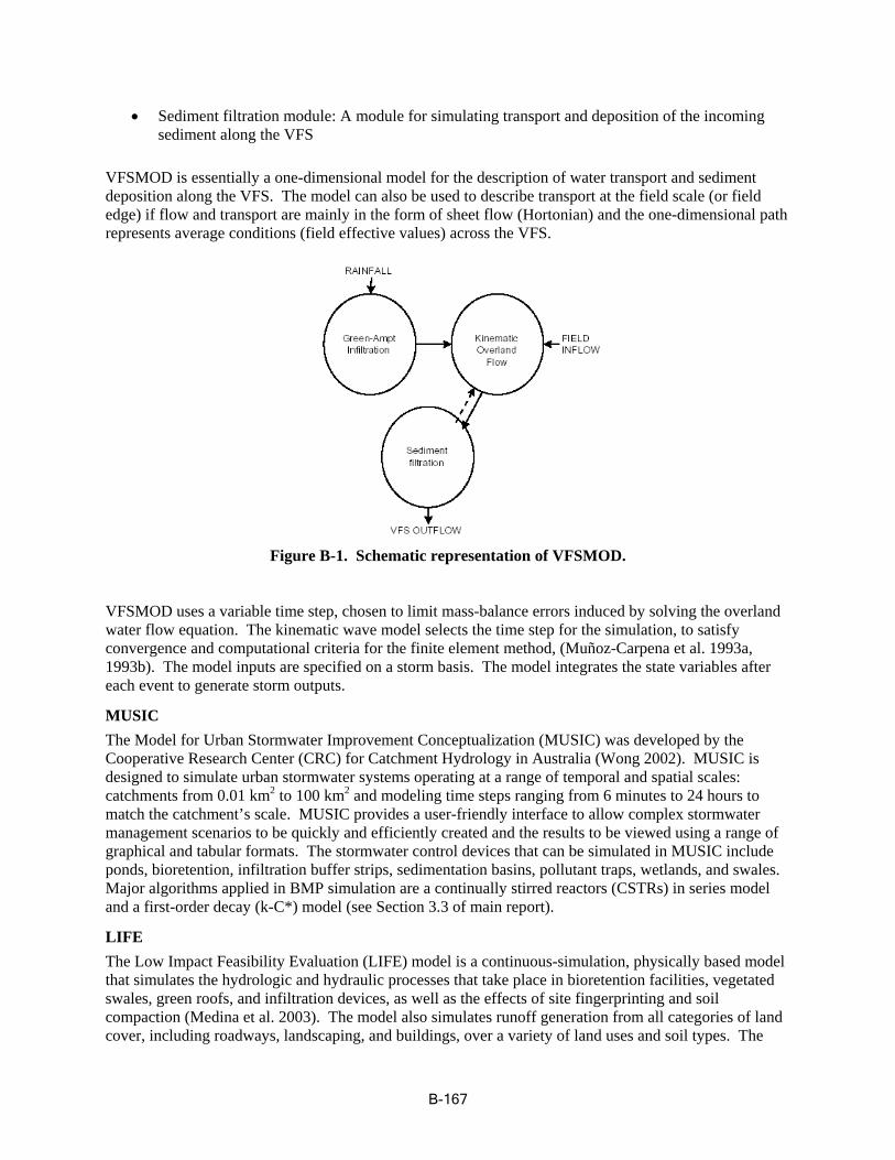
• Sediment filtration module: A module for simulating transport a nd deposition of the in coming sediment along the VFS

VFSMOD is essentially a one-dimensional model for the description o f water transport and sediment deposition along the VFS. The model can also be used to describe transport at the field scale (or field edge) if flow and transport are mainly in the form of sheet flow (Hortonian) and the one-dimensional path represents average conditions (field effective values) across the VFS.

Figure B-1. Schematic representation of VF SMOD.

VFSMOD uses a variable time step, chosen to limit mass-balance errors induced by solving the overland water flow equation. The kinematic wave model selects the time step for the simulation, to satisfy convergence and computational criteria for the finite element method, (M uñoz-Carpena et al. 1993a , 1993b). The model inputs are specified on a storm basis. The model integrates the state variables after each event to generate storm outputs.

MUSIC The Model for Urban Stormw ater Improvement Conceptualization (MUSIC) was developed by the Cooperative Research Center (CRC) for Catchment Hydrology in Australia (Wong 2002). MUSIC is designed to simulate urban stormwater systems operating at a range of temporal and spatial scales: catchments from 0.01 km2 to 100 km2 and modeling time steps ranging from 6 minutes to 24 hours to match the catchment’s scale. MUSIC provides a user-friendly interface to allow complex stormwater management scenarios to be quickly and efficiently created and the results to be viewed using a range of graphical and tabular formats. The stormwater control devices that can be simulated in MUSIC include ponds, bioretention, infiltration buffer strips, sedimentation basins, pollutant traps, wetlands, and swales. Major algorithms applied in BMP simulation are a continually stirred reactors (CSTRs) in series model and a first-order decay (k-C*) model (see Section 3.3 of main report).

LIFE The Low Impact Feasibility Evaluation (LIFE) model is a continuous-simulation, physic ally based model that simulates the hydrologic and hydraulic processes that take place in bioretention facilities, vegetated swales, green roofs, and infiltration devices, as well as the effects of site fingerprinting and soil compaction (Medina et al. 2003). The model also simulates runoff generation from all categories of land cover, including roadways, landscaping, and buildings, over a variety of land uses and soil types. The

B-167

LIFE model is a visually oriented, interactive tool developed on an ExtendTM dynamic simulation platform. The LIFE model is a proprietary model and its modeling details are not available for review.

IDEAL The Integrated Design and Evaluation Assessment of Loadings (IDEAL) model is a spreadsheet model for assessing the impact of BMPs in urban areas on discharge of water, sediment, nutrients, and bacteria into streams (Barfield 2002). The model predicts effluent loads and concentrations of the above elements coming from the watershed as impacted by vegetative filter strips, dry detention ponds, and wet detention ponds. The IDEAL model is capable of estimating the runoff and pollutant loadings from urban areas, categorized into pervious, impervious connected, and impervious unconnected areas. Flows and loadings are summed and then directed to a pond that can be dry (no permanent pool) or wet (permanent pool). The model routes these loadings through BMPs to determine pollutants removal efficiencies using empirical technologies that have been experimentally validated. The model predicts single storm values and converts them to average annual storm values using stochastic procedures. The IDEAL model is designed to estimate BMP long-term pollutant removal efficiencies and is not intended to be used to give accurate estimation on a storm event basis.

DMSTA (Dynamic Model for Stormwater Treatment Area) Model DMSTA simulates daily w ater and mass balances in a user-defined series of wetland treatment cells, each with specified morphometry, hydraulics, and phosphorus cycling parameters (Kadlec and Walker 2003) . Up to six treatment cells can be linked in series and/or parallel to reflect compartmentalization and management to promote specific vegetation types. Each cell is further divided into a series of CSTRs to reflect residence time distribution. Water-balance terms for each cell include inflow, bypass, rainfall, evapotransportation, outflow, seepage in, and seepage out. Parameter estimates for the phosphorus cycling model have been developed for various vegetation types. Water column storage, solid (biomass, sorption) storage, uptake, recycle, and permanent burial processes are considered in dynamic phosphorus cycling simulation. The model is coded in Visual Basic for Applications and the user interface is a Microsoft Excel workbook.

WETLAND The WETLAND model is a dynamic compartmental model to simulate hydrologic, water quality and biological processes, and to assist the design and evaluation of wetland. The W ETLAND model adopted the continuous stirred-tank reactor (CSTR) prototype, and it is assumed that all incoming nutrients are completely mixed throughout the entire volume. The model can simulate both free-water surface (FWS) and subsurface flow (SSF) wetlands. The WETLAND model is constructed in a modular manner, and it includes hydrologic, nitrogen, carbon, dissolved oxygen, bacteria, sediment, vegetation, and phosphorous submodels. The hydrologic submodel uses a vertical dynamic water budget approach to calculate surface storage, and carries out the computation at hourly time step. The factors considered in the hydrologic model include inflow, precipitation, infiltration, and evapotranspiration. The Nitrogen submodel simulates ammonification, immobilization, nitrification, denitrification, and peat accumulation, and inclusion of NH3 volatilization, atmospheric deposition and N fixation in the modeling of overall N cycle is optional. Sorption of NH4

+ to the soil and organic matter is not modeled because it is assumed that sorbed NH4

+ is still available to the attached microbes. The carbon model includes five variables: biomass C, standing dead C, particulate organic C, dissolved organic C, and refractory C; The standing dead C and biomass C is connected to the vegetation submodel. The dissolved oxygen submodel track the oxygen influx from incoming stream flow, precipitation, reaeration from atmosphere, point sources, and biomass flux. In addition, oxygen is assumed to be passed from vegetation stand to wetland bottom at a constant rate during the growing season. The bacteria submodel accounts for all the microbial growth and activity in the model. Both autotrophic and heterotrophic bacteria are modeled. Sedimentation is modeled in the sediment sub-model. The processes simulated include inflow, outflow, deposition, resuspension, and decomposition. Up to five different sediment classifications can be modeled. A simple

B-168

vegetation submodel is included to simulate the biomass growth and death. The phosphorous submodel considers four pools for the P cycle: particulate and dissolved for both the surface and bottom layer of the wetland. Processes modeled in the phosphorous model include mineralization and additions from biomass decomposition. Besides the hydrologic submodel, all the other submodels compute using daily time step.

The strength of the WETLAND model lies on the linked Monod kinetics for the water quality variable s, also the model accounts for the seasonal variation by allowing users to change parameter values for different season/time period. The weaknesses of this model include the completely mixed assumption, which overlook the effect of the system shape, and the needs for extensive kinetic parameters.

VAFSWM The Virginia Field Scale Wetland Model (VAFSWM) is a field scale model for quantifying the pollutant removal in a wetland system. It includes a hydrologic subroutine to route flow through the treatmen t system; Precipit ation, evapotranspiration, and exchange with subsurface groundwater are considered in the hydrologic balance. The model adopted a continuous stir tank system in series schema. VAFSWM models mechanisms of settling, diffusion, adsorption to plants and substrate, and vegetative uptake for a pollutant in dissolved and particulate forms in a two segment (water column and substrate), two state (completely mixed and quiescent) reactor system by employing first-order kinetics. The governing equations for quiescent condition are identical to that of turbulent condition, however far lower settling velocities are assumed to account for the greater percentage of finer particles during the quiescent state.

The VAFSWM is a relatively simple model that includes the most dominant processes within the wetland system. However, the users need to provide and calibr ate the requisite kinetics parameters.

REMM Riparian Ecosystem Management Model (REMM) has been developed as a tool that can help quantify the water quality benefits of riparian buffers. REMM simulates the movement of surface and subsurface water movement, sediment transport and depositio n, nutrients transport, sequestration, and cycling, as well as vegetative growth in riparian forest systems on a daily time step. In REMM, the riparian system is considered to consist of three zones between the field and the water body . Each zone includes litter and three soil layers, and a plant community that can have six plant types in two canopy levels. REMM can be used to quantify nitrogen and phosphorous trapping in riparian buffer zone, determine buffer effectiveness, investigate long-term fate of nutrients in buffer zones and, evaluate influence of vegetation type on buffer effectiveness, and determine impacts of harvesting on buffer effectiveness.

The strength of REMM is its capability of simulating subsurface compartment, and the comprehensive nutrients cycling. Comes with the complexity, one disadvantage of the model is the extensive data requirement. REMM is still under development and has been continuously updated. Currently, a user interface is being built to assist input and output data management.

B.3.3. Modeling System Reviews Several systems have been developed that include multiple models and software systems to facilitate d ata storage, data preparation, model input file development, model application and linkages, and output post­processing. These comprehensive systems have the potential for integration or communication with SUSTAIN. As these system s continue to evolve, SUSTAIN will consider options to preserve compatibility with these systems.

B-169

BASINS Better Assessment Science Integrating point and Nonpoint Sources (BASINS), developed by EPA, is a multipu rpose environmental analysis system for use by regional, state, and local agencies in performing watershed and water quality based studies (USEPA 2001). BASINS has three major objectives: (1) to facilitate examination of environmental information, (2) to support analysis of environmental systems, and (3) to provide a framework for examining management alternatives.

BASINS integrates a GIS, national watershed and meteorological data, and state-of-the-art environmental assessment and modeling tools into one convenient package. Originally released in 1996, with a second release in 1998, a third in 2001, and a fourth in 2004, BASINS comprises a suite of interrelated compon ents. The current version is BASINS 4.0.

In a departure from previous versions, BASINS 4.0 databases and assessment tools run on a non­proprietary, open source GIS system architecture (MapWindow). Its components work together to support the user in performing various aspects of environmental analysis. The components include (1) nationally derived databases with Data E xtraction and Project Builder tools; (2) assessment tools (TARGET, ASSESS, and Data Mining) that address large- and small-scale characterization needs; (3) utilities to facilitate importing local data and to organize and evaluate data; (4) Watershed Delineation tools; (5) utilities for classifying elevation (DEM), land use, soils, and water quality data; (6)Watershed Characterization Reports that facilitate compilation and output of information on selected watersheds; (7) an in-stream water quality model; (8) two watershed loading and transport models; and (9) a simplified GIS-based, nonpoint annual loading model. Installed on a personal computer, BASINS allows the user to assess water quality at selected stream sites or throughout an entire watershed. The software makes it possi ble to quickly assess large amounts of point source and nonpoint source data in a format that is easy to use and understand, as well as to prepare and set up watershed and in-stream transport models to facilitate the TMDL analysis for waterbodies of concern.

A limitation of the current BASINS configuration is that data currently housed in the BASINS system is typically too general to support detailed urban analysis. The system data would need be updated with local data to facilitate application and provide higher resolution analysis necessary for SUSTAIN. For more information, see the BASINS Web site (see http://www.epa.gov/waterscience/basins/ ).

EPA TMDL Modeling Toolbox The TMDL Modeling Toolbox is a collection of models, modeling tools, and databases that have been widely applied over the past decade in the development of TMDLs. The Toolbox takes those proven tech no logies and provides the capability to more readily apply the models, analyze the results, and inte gra te watershed loading models with receiving water applications (USEPA 2003). The design of the Toolbox is such that each of the models is a standalone application. The Toolbox provides an exchange of information between the models through common linkages. The modular design of the Toolbox allo ws for additional model s to be easily incorporated and integrated with the other tools. In addition, the Toolbox provides the capability to visualize model results, a linkage to GIS and nongeographic databases (including monitoring data for calibration), and the functionality to perform data assessments.

The Toolbox allows for the steady-state/dynamic simulation of mass transport and water quality processes in all types of surface water environments, including overland flow, small creeks, rivers, lakes, estuaries, coastal embayments, and offshore areas. The Toolbox contains assessment tools, watershed models, and rece ivi ng water models, including the following:

Assessment Tools

• Water Resources Database (WRDB)

B-170

• Watershed Characterization System (WCS) • WCS Sediment Tool • WCS Mercury Tool • WCS LSPC Tool

Watershed Models

• Loading Simulation Program in C++ (LSPC) • Watershed Assessment Model (WAMView) • Stormwater Management Model (SWMM)

Receiving Water Models

• A Dynamic, One-Dimensional Model of Hydrodyn amics and Water Quality (EPDRiv1) • Stream Water Quality Model (QUAL2K) • CONservational Channel Evolution and Pollutant Transport System (CONCEPTS) • Environmental Fluid Dynamics Code (EFDC) • Water Quality Analysis Simulation Program (WASP)

The Toolbox has a wide variety of included models and open architecture that facilitates linkages and flexibility in application. A limitation of the system is the lack of specific models and tools for simulating BMPs. Although LSPC and WAMView can be used to simulate BMPs, the systems do not include detailed, process-based simulation capabi lities or convenient tools to quickly set up and evaluate alternative BMP management alternatives.

B.4. Discussion and Results of Model Review A review was conducted of a vailable models such as SWMM (Huber and Dickinson 1988; Huber 2001), HSPF (Bicknell et al. 1993), and SLAMM (Pitt and Voorhees 2000), as well as publicly available modeling systems, such as BASINS (USEPA 2001) and the TMDL Modeling Toolbox (Tetra Tech and USEPA 2002). Based on this review, there is no single system or model with the flexibility and capability to incorporate all the technical needs listed below for the SUSTAIN development.

• Ability to simulate hydrologic response and a level of detail sufficient for analysis of a hydrograph (peak flow and volume)

• Ability to simulate multiple pollutant types, including nutrients (nitrogen and phosphorus), pathogens [fecal coliform bacteria, Escherichia coli (E.Coli)] and metals (zinc, aluminum, etc.)

• Ability to simulate fate and transport of pollutants and evaluate both acute and chronic impacts • Ability to generate sediment loading to streams • Ability to simulate sediment transport in streams • Ability to simulate multiple size classes of sediment for input to management structures • Ability to simulate other habitat stressors, such as temperature • Ability to simulate in-stream dissolved oxygen based on inputs of biological oxygen demand,

sediment oxygen demand, nutrient loads, and other environmental factors • Ability to evaluate urban and mixed land uses, including pervious and impervious areas

B-171

• Consideration of short and long time periods (single- and multiple-event simulation) • Consideration of a full range of management practices at a similar level of spatial resolution • Consideration of distributed or small-scale management practices and larger downstream

facilities • Consideration of a series of management practices at various locations in the watershed • Modeling of management practices on a time-variable basis consistent with the need to eva luate

hydr ology and pollutant measures • Ability to consider placement of management practices at any location in the watershed (e.g., at

various distances from waterbodies, at various stream orders) • Ability to link watershed management to downstream measures of environmental condition (e.g.,

dissolved oxygen in a river, nutrient concentration in a lake or estuary) outside the immediate vicinity of a selected study area

However, many models can provide portions of the needed features and algorithms. Comparison of the available models and the technical needs supports selection of a subset of models for further consideration, and their potential incorporation in SUSTAIN is organized according to the key components identified in the preliminary design discussion. Table B-7 summarizes the strengths and weaknesses of the selected watershed models in light of the SUSTAIN design requirements. Presented below is a process-focused summary discussion of the models that supports the landscape and BMP model selection.

B.4.1. Watershed Models The selection of watershed models for integration into SUSTAIN are discussed separately for hydrology, sediment, pollutant loadings, and reach routing.

Hydrology Several watershed models, including SWMM, SLAMM, HSPF, and LSPC, can provide time series hydrology and pollutant loading at an hourly time step or less. This short temporal resolution is needed to address small catchments and to provide concentration and load predictions and time series inputs to management practices. This temporal resolution is necessary for the flexibility to predict the range of hydrologic and water quality measures identified in the needs analysis. Some models, such as SWAT (Neitsch et al. 2001), AnnAGNPS (AnnAGNPS 2000), AGNPS (Young et al. 1986), and GWLF (Haith et al. 1992), are inappropriate because they use large time steps (1 day or greater) or insufficient description of time-variable rainfall-runoff processes. Other models, such as CASC2D and KINEROS, use a grid-based framework for distributed modeling of the watershed landscape. The grid-based formulation has benefits for detailed simulation and sensitivity to the placement of management within the landscape. However, its greatest limitations are high computational needs for larger watersheds and the availability of spatially detailed data. The spatial detail can significantly increase the data preparation and setup time for the model. Currently, CASC2D and KINEROS do not include water quality simulation capabilities. Further evaluation is needed to determine whether cell- or grid-based modeling components can b e incorporated into SUSTAIN. The initial recommendation is to use pervi ous and impervious land simulation routines from SWMM, HSPF, and/or LSPC.

Sediment The HSPF and LSPC watershed models use a sophisticated process-based system to describe sediment simulation for pervious areas and buildup/washoff for impervious areas. For pervious segments, sediment is represented as a direct function of the rainfall intensity. The rainfall intensity determines the rate and volume of material detached from an infinite soil matrix, while the scouring process determines the

B-172

washoff and delivery of sediment to a stream segment. Scour can be used to represent gully erosion. Because this process is energy-driven, the calibration changes with the time step and resolution of the rainfall data driving the system. For impervious land surfaces, both HSPF/LSPC and SWMM use similar approaches to simulate buildup and washoff of solids on the land surface. HSPF and SWMM allow the user to apply special actions, such as street sweeping during the simulation, to assess the impact of such a management activity on the overall delivery of solids from urban streets. SWMM allows three ways for estimating sediment in runoff: (1) a rating curve, (2) a buildup and washoff approach, or (3) the USLE for pervious surfaces.

If the methods described above are compared with another popular sediment estimation method such as USLE (which is used by many of the models described in Section A.3), some limitations, in light of the project requirements, are evident. The parameters feeding the USLE equation are based on long-term assessments, and the results, though meaningful as a monthly or annualized loading estimate, fail to adequately represent the detailed variability of individual storms or storms in series. In conclusion, short/variable time step methods, such as those available in HSPF and LSPC for pervious areas and in SWMM, HSPF, and LSPC for impervious areas, are better suited to satisfy the assessment objective s outlined for SUSTAIN.

Pollutant Loading Among the shorter/variable-time-step simulation models like SWMM, HSPF, and LSPC, buildup and washoff of pollutants on a land surface is often used as the primary process for generating pollutant loadings. In HSPF and LSPC, pollutan ts can also be represented as sediment-associated; therefore, some of the pollutant mass will be considered as a fraction of the simulated sediment delivery. Base flow and interflow concentrations in HSPF and LSPC are specified as constants, or they can be expressed as monthly variable concentrations. SWMM does not allow for a variable buildup rate; however, it allow s the user to specify the equation and method used (power-linear, exponential, or Michaelis-Menton). As with sediment, SWMM allows for pollutants to be specified as a function of the flow rating curve or by using buildup and washoff. Pollutants can also be associate d with sediment by expressing the mass as a fraction of sediment. Simpler models, such as GWLF and P8, use a fixed concentration of a pollutant in runoff and sediment, making them insensitive to changes in concentration or availability of pollutants over time. These models also use daily or monthly time steps, and they cannot support the evaluation of short-duration loading and impacts on stream systems. For pollutant loading, HSPF, LSPC, and SWM M include the preferred techniques for integration into the SUSTAIN design.

Reach Routing Landscape output must also be collected and routed via flow networks (channels and streams). Many watershed mod els, including SWMM and HSPF, include stream routing modules. These routing techniques, which involve some simulation of in-stream transport and pollutant transformation processes, are sufficient for smaller streams with relatively short conveyance times (less than 1 day). Urban streams typically have short retention times an d limited opportunity for biological and chemical processes to result in significant transformation of pollutants. Of the reviewed models, HSPF and LSPC reach routin g have the most detailed simulation capabilities for sediment and pollutant transport including sed iment deposition, scour, decay, and dynamic temperature simulation. SWMM’s transport functions include first-order decay and settling but do not include an option for temperature, biological transformation, or algal growth. SWMM can simulate complex hydraulics using a fully dynamic wa ve method. For areas with large, longer-retention-time river systems or tidally influenced systems, an external linkage (outside SUSTAIN) can provide the ability to evaluate downstream impacts. Linkage with specialized receiving water models, such as EFDC (Hamrick 1992) and WASP 6.0 (Wool et al. 2003), ultimately can be used to consider the impacts of urban stormwater runoff on larger, more complex waterbodies. Specialized receiving water models like WASP (Wool et al. 2003) are also best suited for evaluating eutrophicatio n processes and dissolved oxygen.

B-173

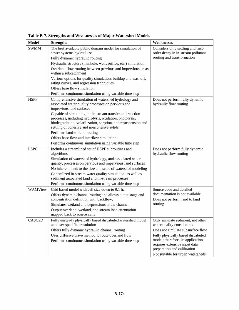
Table B-7. Strengths and Weaknesses of Major Watershed Models Model Strengths Weaknesses SWMM The best available public domain model for simulation of

sewer systems hydraulics: Fully dynamic hydraulic routing Hydraulic structure (manhole, weir, orifice, etc.) simulation Overland flow routing bet ween pervious and impervious areas within a subcatchment Various options for quality simulation: buildup and washoff, rating curves, and regression techniques Offers base flow simulation Performs continuous simulation using variable time step

Considers only settling and fir order decay in in-stream pollu routing and transformation

st­tant

HSPF Comprehensive simulation of watershed hydrology and associated water quality processes on pervious and impervious land surfaces Capable of simulating the in-stream transfer and reaction processes, including hydrolysis, oxidation, photolysis, biodegradation, volatilization, sorption, and resuspension and settling of cohesive and noncohesive solids Performs land-to-land routing Offers base flow and interflow simulation

stepPerforms continuous simulation using variable time

Does not perform fully dynam ic hydraulic flow routing

LSPC Includes a streamlined set of HSPF subroutines and algorithms Simulation of watershed hydrology, and associated water quality, processes on pervious and impervious land surfaces No inherent limit to the size and scale of watershed modeling Generalized in-stream water quality simulation, as well as sediment associated land and in-stream processes Performs continuous simulation using variable time step

Does not perform fully dynamic hydraulic flow routing

WAMView Offers dynamic channel routing and allows outlet stage and concentration definition with backflow.

Grid based model with cell size down to 0.1 ha

Simulates wetland and depressions in the channel Output overland, wetland, and stream load attenuation mapped back to source cells

Source code and detailed entation is not available ot perform land to land

docum Does n routing

CASC2D Fully unsteady physically based distributed watershed model

outing Uses diffusive wave method to route overland flow

at a user-specified resolution Offers fully dynamic hydraulic channel r

Performs continuous simulation using variable time step

Only simulate sediment, not other

Does not simulate subsurface flow Fully physically based distributed

ta

water quality constituents

model; therefore, its application requires extensive input da preparation and calibration Not suitable for urban watersheds

B-174

B.4.2. BMP/LID Models Simulation of BMPs varies between simplified representation of percent removal and partial or complete representation of the processes of hydraulic controls, settling, and transformation of pollutants. A number of available watershed models have the potential for use in BMP simulation (e.g., SWMM, HSPF, LSPC , and SLAMM), but representation is achieved by custom adjustment of hydrologic and pollutant transpo rt parameters. Guidance for the application of watershed models such as SWMM and HSPF for simulation of BMPs is limited. Consistent application is difficult, and in the absence of default data and docum ented applications, intensive data collection and calibration are necessary. Some models, such as WAMView, can be adjusted to represent land practice BMPs based on the USDA Curve Number guidance. Many of the currently available, published BMP models are propriety (e.g., MUSIC) or have had limited releas e in the public domain (e.g., BMPAM). Specialized BMP simulation tools such as VFSMOD (Muñoz-Carpena and Parsons 2003) focus on specific BMPs, in this case vegetative filter strips.

Most of the currently available systems have limited process simulation or lack guidance for the selection and evaluation of management practices. Of the available systems, the Prince George’s County BMP Module provides capabilities to simulate a wide range of BMPs with particular emphasis on scale-scale, distributed systems, using a process-based approach to address h ydrology and pollutant removal. One specialized need for BMP simulation is the ability to handle highly distributed management techniques such as those employed in LID procedures. The Prince George’s County BMP Module was designed specifically to address LID simulation and networks with multiple mana gement practices. The structure of the BMP Module can facilitate the incorporation of additional BMP types and is suitable for linkage with a variety of watershed and receiving water models. Prince George’s County has provided the system to users upon request and is willing to provide EPA with the code for adaptation and incorporation into SUSTAIN.

For the process simulation of BMPs, the Prince George’s County BMP Module, augmented by portions of selected BMP processes provided by models such as SWMM, SLAMM, and P8, is recommended for incorporation into SUSTAIN. In particular, BMP simulation techniques for stormwater ponds and detention structures can be provided by SWMM. For BMPs such as riparian buffers, specialized simulation techniques are also needed. Riparian buffers can be addressed by using the procedures in VFSMOD (Muñoz-Carpena and Parsons 2003) or by adapting the land-to-land transport routines used in SWMM or HSPF.

B.5. Conclusions The review of available models and BMP analysis systems confirms the initial selection in Task 1 of a short list of models best suited to be included in the SUSTAIN system. The final recommended list of models was based on an evaluation of the needs, the level of analysis included, the software capabilities, and the availability of the code supporting the models. Each of these models provides essential software tools; algorithms describing watersheds, receiving waters, or BMP processes; and a history of application and testing. In addition, existing models can be linked with SUSTAIN for combined simulation of la rge, complex watersheds and receiving waters. The selected models are the following:

• Watershed/landscape models: SWWM, HSPF, LSPC • Stream conveyance and pol lutant routing models: HSPF/LSPC stream routing and pollutant

transport functio ns, or SWMM routing and transport (SWMM5) • Stream conduit (combined sewer overflow, or CSO) models: SWMM

B-175

• BMP simulation models: Prince George’s County BMP Module, including new algorithms for detention ponds and structural options, and selected buffer zone simulation techniques from VFSMOD

Dev elo pment of the system will also require a framework manager, and supporting GIS tools, optimiz ation, cost estimation, and post-processing techniqu es. The relevant components of the selected mod els, supporting algorithms, and tools will be integrated in to a seamless framework that can provide the required functionality.

B-176

C

Appendix C. Summary of the Optimization Technica l Panel Meeting

C.1. Background Watershed and stormwater managers need modeling tools to ev aluate how best to address environmental quality restoration and protection needs in urban and developing areas. A place-based analysis system, based on cost optimization, is essential to support government and local watershed planning agencies as they coordinate efforts across the watershed to achieve desired improvements in water quality at a minimum cost.

A two-day workshop was convened September 15-16, 2006, at the Fairfax, Virginia, office of Tetra Tech, Inc., to bring together experts to discuss the current state-of-the-art in optimization concepts and methods to support development of the optimization component in SUSTAIN. The invited experts included the following:

• Dr. James P. Heaney (University of Florida) • Dr. Manuel Laguna (University of Colorado) • Dr. Arthur E. McGarity (Swarthmore College) • Dr. S. Ranji Ranjithan (North Carolina State University) • Dr. Christine A. Shoemaker (Cornell University) • Dr. Richard M. Vogel (Tufts University) • Dr. Laura J. Harrell (Old Dominion University)

Optimization decision variables include BMP locations, types and design configurations. Because there can be an extremely large number of possible combinations of BMP choices that can meet desired water quality and quantity constraints, strategies are needed to identify specific BMP options for implem entation from a vast output database. The primary objective of the workshop was to identify t he best strategies available for implementation in SUSTAIN. A secondary objective of the workshop was to discuss and report issues related to cost estimating and in defining and quantifying the effectiveness of individual BMPs or several BMPs in parallel or in series. This appendix is a summary of the workshop discussion and recommendations.

C.2. Key Discussion Issues The workshop focused on discussing and acquiring experts’ knowledge on issues listed below in four categories:

C.2.1. General Issues • Trend and focus - What are the current trends and focus in optimization research for watershed

planning?

C-177

• Algorithm selection and evaluation – It was proposed to program two search algorithms in SUSTAIN: 1) Scatter Search and 2) genetic algorithm. Which one is more robust in providing placement decisions? Should other solution techniques be considered? How can it be confirmed that global or near global solutions have been found?

C.2.2. Optimization Approach • Two-tier approach – Presumably a tiered optimizatio n approach will facilitate placement of

BMPs in different spatial scales. Can a two-tier or cascading optimization approach work to develop large scale solutions? BMPs may be placed at the site scale or subwatershed scale, but overall control performances are evaluated at the watershed scale

• Top down vs. bottom up - Should a watershed optimization process be top-down (from the watershed to subwatershed to site scales) or bottom-up?

C.2.3. Computational Efficiency • Aggregation of distributed BMPs - BMPs include distributed types such as green roofs,

bioretention basins, porous pavements and rain barrels. What are the most efficient solution strategies and computational approaches to simulate and optimize hundreds of distributed BMPs? How should the distributed BMPs be lumped (usually at p arcel scales)? How should the BMP clusters be represented by lumped hydrologic parameters (e.g., depression storages and infiltration rates)?

• Simplified approach to derive effectiveness from multiple BMPs - BMPs can be in series or in parallel in a given subwatershed. It will be computationally demanding if process simulations are performed for each combination of treatment trains. Can experiments be performed to establ ish a database for deriving a regression formula that can be used to estimate the pollutant load reduction from all possible combinations of BMPs?

• Development of cost-effectiveness curves – What is the most efficient way to generate cost-effectiveness curves (cost vs. effectiveness) when using meta-heuristic algo rithms? The curve can be derived from multiple costs vs. load reduction points by simulating multiple runs under a range of load reduction targets. This option will be computationally time-consuming because a large number of simulation runs may be required to derive multiple o ptimal solutions

C.2.4. Problem Formulation - Objectives, Constraints and Variables • Pollution vs. flood control objectives - How to reconcile the potential conflicts between meeting

pollution control and flood control objectives? The pollution control effectiveness is usually assessed by a continuous simulation, while flood control effectiveness is assessed by an event simulation

• Multiobjective optimization - How should the objective equation be formulated? • Future land use management - Is the future land use manag ement a decision variable in the

BMP placement decision? In other words, should the land use planning and water quality management be integrated? SUSTAIN is designed for placing BMPs in watersheds with known existing or future land uses

• Cost estimating - For estimating the cost of BMPs, what will be the level of detail required to maintain the consistency of decision parameters used in optimization analyses?

• Financial resources and implementation schedule – How to include constraints on financial resources and schedules of BMP implementation in the optimization framework?

C-178

C.3. Discussion Summary This section summarizes the discussion and input from the invited experts, organized by the discussion issues.

C.3.1. General Issues Trend and focus - What are the current trends and focus in optimization research for watershed plannin g?

An eme rging trend is to apply optimization techniques, especially meta-heuristic algori thms, to solve stormwater management issues. Although a number of research projects have been completed in recent years, most of them are conducted in academia and most of them were developed on a case-by-case basis. There has not been any generic decision support system developed that can be used by a general public practitioner to optimize size, type and locations of BMPs.

During the discussion, the application of neural networks and parallel computing for the purpose of reducing search time was brought up. Although there are uncertainties that neural networks can accurately represent the real simulation module with limited training process, it was suggested that they can be used as a filter during the search process to avoid spending CPU time to evaluate bad solutions. Parallel computing can be employed where a network of computers is available to use all possible resources to obtain the search results in a shorter time.

A hybrid approach of combining traditional and meta-heuristic algorithms can be promising as traditional algorithms are more efficient for reaching local optima and meta-heuristic algorithms have the advantage of not b eing trapped at the local optima.

Algorithm selection and evaluation - It was proposed to program two search algorithms in SU STAIN: 1) Scatter Search and 2) genetic algorithm. Which one is more robust in providing pl acement decisions? Should other solution techniques be considered? How can it be confirmed that global or near globa l solutions have been found?

There is no quick answer for the question of which algorithm is better than the other. In terms of solution techniques, it was mentioned that Evolution Strategies are claimed to be faster at numerical optimization than traditional Genetic Algorithms. A participant presented a stochastic RFB-Cornell radial basis function approach and showed it converged significantly faster than a few other techniques for a particular case study she conducted. The participant also suggested that the alternatives for optimiza tion algorithms need to be evaluated carefully since the simulation time can be substantial. It was also note d that using commercial software Solver associ ated with spreadsheet analysis could be an efficient alternative. Other participants also found commercial software useful for testing new search algorithms.

To address the question of how to confirm that global optima has been found, the experts agreed that, theoretically, global optima cannot be proved when using meta-heuristic techniques. That is why the term near optimal should always be used instead of optimal. However there are a few ways to help gain confidence:

• Use a benchmark test case with known optima • Compare and try different solution techniques • Use commercial software to compare results

C-179

Another way of looking at the near optima is that although it is not guaranteed to be the optima, they are better than the other solutions that have been checked during the search process. This leads to the suggestion that starting the search with a good solution might result in the near optimal solution faster. It was pointed out that local optima can be proved by checking the derivative if the problem is continuous.

Other than one member, the invited experts appeared unfamiliar with the Scatter Search method. Two experts both talked at several times about the potential utility of traditional dynamic programming techniques.

The workshop experts demonstrated the following optimization applications that can be further explored:

One expert talked about the experience of using Genetic Algorithm (GA) to optimize the locations of infiltration practices for reducing peak flow. A curve number (CN)-based distribution model was used to simulate the hydrological responses and infiltration BMPs are represented as change of CN. A series statistical analysis was performed to check if there is another way to identify the optimal BMP locations without using optimization. The results were negative; this confirmed the need for applying optimization techniques to get the cost-effective solutions for stormwater management issues. It was also commented that a decision support system does not necessarily provide BMP design details as part of the solution; instead it is only necessary to suggest the general categories of BMPs and the expected treatment (i.e., infiltration and/or storage) capacity. In addition, sometimes simplified optimization such as Linear Programming (LP) may give results that are comparable to GA solutions. The following web site was suggested to download papers and manuscripts for more detail: (http://ase.tufts.edu/cee/faculty/vogel/bio.asp ).

Another expert presented a spreadsheet optimization tool that used the Excel add-on optimization engine Solver to find cost-effective BMPs. The BMPs were represented as a combination of on-site depression storage (DS) and/or centralized storage/release systems.

A third expert showed Storm Water Investment Strategy Evaluator (StormWISE), which is a screening level stormwater management optimization tool. This tool employs a top-down approach to prioritize investm ent in subwatersheds for pollution control. The essential component of this tool is the generaliz ed pollutant-removal/cost functions for each land use in each subwa tershed (first-stage). The functions are then used for the second-stage optimization. As the pollutant-removal/cost functions are well-behaved, a classical optimization technique, mixed integer/linear programming, is used to solve the second-stage optimiz ation problem. The following Web site (http://watershed.swarthmore.edu) has more details.

Two panelists pointed out the importance of providing diverse alternative solutions. One presented a case study where an evolutionary algorithm was applied to obtain diversified alternative solutions that have comparable objective values. It was emphasized that the approach was efficient because it was perf ormed along the search process for the main optimization problem so that it did not require to rerun the model. Another expert also commented that ther e might often be multiple feasible solutions within a very small percentage of benefit or cost range. In that case the system needs to identify the most diversified alternatives that the user can choose from (using their own judgment).

C.3.2. Optimization Approach Two-tier approach - It is believed that a tiered optimization approach will facilitate placement of BMPs in different spatial scales. Can a two-tier or cascading optimization approach work to develop large scale solutions? BMPs may be placed at the site scale or subwatershed scale, but overall control performances are evaluated at the watershed scale.

C-180

Overall, the experts agreed that the tiered approach is promising; however, they foresee the obstacle of daunting computation time if the meta-heuristic optimization algorithm is employed. A few ideas came up during the discussion. The first group of ideas focused on reducing the complexity of the simulation system by either employing a simpler and faster simulation approach or by using a generic cost-pollutant­removal function to eliminate the needs of detailed BMP simulations. The second group of suggestions focused on improving optimization efficiency. One expert mentioned the use of dynamic programming (DP) for the second tier analysis. If applicable, DP can be more efficient than meta-heuristic algorithms. However, it is recognized that implementing DP in a decision support system such as SUSTAIN, which is intended to be applicable to many different cases, would be difficult because DP requires a case-by-case problem formulation. Another suggested using neural networks as a filter during the optimization process to avoid spending time in evaluating bad solutions.

Top down vs. bottom up - Should a watershed optimization process be top-down (from the watershed to subwatershed to site scales) or bottom-up?

The top-down approach involves applying generalized cost-benefit functions (such as the pollutant-removal/cost functions in StormWISE) to prioritize the distribution of load reduction requirements at the subwatersheds, given a target at the watershed level. The advantage of this approach is that an efficient classical optimization algorithm can be used because the generalized cost-benefit functions are smooth and convex. The challenge of this approach is to obtain reasonably accurate cost-benefit functions. If the cost-benefit function is not accurate, the solutions can be skewed. Also, this approach does not explicitly address BMP implementation details.

For the bottom-up approach, the search starts with the potential locations identified; therefore it explicitly addresses the BMP implementation details. The downside of this approach, as commented on by one expert, is that the amount of site-specific information and data required for specifying sites and potential BMPs could be prohibitive. Also, the approach is simulation intensive and when it is applied for a large watershed the computation time required can be extensive.

From discussions, a strategy that combines bottom-up and top-down procedures appears promising. The overall optimization process can start with the top-down approach as applied in StormWISE using generic cost-benefit functions to identify the high priority subwatersheds, then perform a detailed bottom-up optimization search for each priority subwatershed to derive a more accurate and site-specific cost-benefit curve. By doing so, the computation time is expected to be reduced because detailed simulation/optimization is conducted only for the priority subwatersheds. The search process is then completed with another round of top-down optimization using the cost-benefit functions derived from the previous step.

C.3.3. Computational Efficiency Aggregation of distributed BMPs - BMPs include distributed types such as green roofs, bioretention basins, porous pavements and rain barrels. What are the most efficient solution strategies and computational approaches to simulate and optimize hundreds of distributed BMPs? How should the distributed BMPs be lumped (usually at parcel scales)? How should the BMP clusters be represented by lumped hydrologic parameters (e.g., depression storages and infiltration rates)?

One participant presented the approach of using aggregated depression storage to represent the site-scale or distributed BMPs (such as green roofs, porous pavement, rain-gardens, etc.) at the catchment level. Another suggested using response functions to represent distributed BMPs at the scale of a neighborhood or region of an urban area. The response functions need to be in the form of simplified formulations

C-181

derived from regressions or theoretical means. It was suggested that a highly detailed simulation model driven by an optimizer can be used to generate data for curve fitting.

Simplified approach to derive effectiveness from multiple BMPs - BMPs can be in series or in parallel in a given subwatershed. It will be computationally demanding if process simulations are performed for each combination of treatment trains. Can experiments be performed to establish a database for deriving a regression formula that can be used to estimate the pollutant load reduction from all possible combinations of BMPs?

This topic was discussed under aggregation of distributed BMPs.

Development of cost vs. effectiveness curves - What’s the most efficient way to generate cost-effectiveness curves (cost vs. effectiveness) when using meta-heuristic algorithms? The curve can be derived from multiple cost vs. load reduction points by simulating multiple runs under a range of load reduction targets. This option will be computationally time-consuming because a large number of simulation runs may be required to derive multiple optimal solutions.

One participant suggested that the cost-effectiveness curve can be developed in a continuous search at various target values without stopping the search. The process can start with solving the optimization problem with the highest target value. After getting the near-optimal solutions, relax the target and resume the search. The previous solutions are kept and can be selectively used to construct the reference set for the subsequent searches.

Simplification of the Channel/Pipe Routing Simulation Channel/pipe routing is computationally extensive because it employs the kinematic wave flow routing method. To reduce the computation burden, it is desirable to simplify the routing simulation during optimization runs and only use the kinematic wave approach for evaluation runs. The possible simplified routing options include, but are not limited to:

• Adopt the simple approach of steady flow routing (from the SWMM) for the optimization runs • Pre-run the routing module with kinematic wave approach to build a stage-discharge relationship

and then use that relationship during the optimization runs

C.3.4. Problem Formulation - Objectives, Constraints and Variables Pollution vs. flood control objectives - How should the potential conflicts between meeting pollution control and flood control objectives be reconciled? The pollution control effectiveness is usually assessed by a continuous simulation, while flood control effectiveness is assessed by an event simulation.

One participant suggested to address flood control objectives by penalizing corresponding solutions if flooding occurs during the long-term simulation.

Another expressed the idea of using goal programming. The approach should be to solve the event-based flood control problem first and then, in most cases, the solution for the pollutant control will be automatically included in it. Otherwise it is necessary to add extra dimensions in the optimization problem formulation. Someone also mentioned that in urban land uses first-flush may be the main cause of pollution, but in rural areas the larger storm events may be the major factor because of erosion. It was commented that in suburban situations there will be a combination of both, therefore, both situations should be addressed. It was suggested that one approach could be to include flood control considerations as part of the screening stage of the analysis (i.e., narrow the search for water quality BMP’s to the subwatershed drainage areas where flood frequency is high). Another participant commented that

C-182

although extreme events may be a major source of pollution or erosion, no BMPs are designed to handle catastrophic events.

Multiobjective Optimization – How should the objective function be formulated? The need for multiobjective optimization was recognized. Formulation was discussed in the context of sequential analysis or various supplementation analyses of the near optimal solutions. No specific recommendations were made on the solution of multiple objectives, although time and complexity constraints were recognized.

Future land use management - Is the future land use management a decision variable in the BMP placement decision? In other words, should the land use planning and water quality management be integrated? SUSTAIN is currently designed for placing BMPs in watersheds with known existing or future land uses.

It was noted that land use planning can have an implicit impact on the stormwater management solutions. For example, aggregating the development areas, which have a larger percentage of imperviousness, can increase the cost-effectiveness of stormwater control practices.

Cost estimating - For estimating the cost of BMPs, what will be the level of detail required to maintain the consistency of decision parameters used in optimization analyses?

One participant commented that the cost function is very important in decision-making and mostly overlooked. LIDs make the cost estimation difficult because many LIDs have multiple purposes. CAPITA, a wastewater treatment database, was mentioned for cost estimation. This database contains realistic cost data for mostly conventional treatment units. It was also pointed out that it is difficult to estimate the land cost. Another suggested that if the actual cost data were not available, then as long as the relative costs were correct, the solutions would still be valid. It was suggested that the SUSTAIN system allows the flexibility for users to use default data or enter locally derived cost information.

Another participant mentioned that it might be useful to use resources consumed as the surrogate for cost.

Financial resources and implementation schedule - Should constraints on financial resources and schedules of BMP implementation be included in the optimization framework?

It was recognized that the system does not need to include schedules of BMP implementation because the BMP options are discrete and solutions for the next target may not be inclusive of the solutions derived under the current goal. An example was goven where there is a choice between large structures versus small distributed systems. The funding limitation can drive the solution to either implementing the distributed or the centralized systems, then the solutions are mutually exclusive. When there is a need for next phase planning a separate optimization should be performed based on the future conditions.

It was commented that it is desirable to formulate the optimization problem as minimizing the cost because if the constraint is the actual budget then the cost function needs to be accurate. Otherwise the solution could be skewed.

C.4. Conclusions The workshop included a thorough discussion of the tiered optimization approach, comparing top-down and bottom-up search strategies. Expert opinions were gathered on how to prove if the optimization solutions are good, if not the best, and how to evaluate and improve the search efficiency.

C-183

In summary, the following items were identified as the major items worth considering in SUSTAIN development and future improvement:

• Combine top-down and bottom-up search strategies for the tiered optimization • Explore the use of classic optimization techniques, such as LP, Nonlinear Programming (NLP)

and DP, for the second tier top-down optimization • Evaluate the employed optimization techniques by:

o using a benchmark test case with known optima o comparing different solution techniques o using commercial software to compare results (below are a few Web sites the experts

have mentioned): � HTUwww.palisade.comUTH Evolver � HTUwww.solver.comUTH Frontline Systems, Inc. � HTUwww.mgc.ac.cn/genomecomp UTH GenomeComp � HTUwww.inria.fr/recherche/equipes/dolphin.en.html UTHDolphin � HTUcsmr.ca.sandia.gov/projects/opt.htmlUTH Sandia

• Provide diverse near-optimal solutions • Represent the distributed or site-scale BMPs using the hydrologic simulation parameters (i.e.,

depression storage and infiltration parameters) • Explore the feasibility and options of applying the simplified channel/pipe routing approach for

optimization runs • Explore the concept of relative cost

C-184

D

Appendix D. Appendix References

Alley, W.M., and P.E. Smith. (1982a). Distributed Routing Rainfall-Runoff Model—Version II. Open File Report 82-344. U.S. Geological Survey, Reston, VA.

Alley, W.M., and P.E. Smith. (1982b). Multi-event Urban Runoff Quality Model. Open File Report 82­764. U.S. Geological Survey, Reston, VA

AnnAGNPS. Technical descriptions. (2000). Hhttp://www.sedlab.olemiss.edu/AGNPS.htmlH. Accessed 2001.

Barfield, B.J., J.C. Hayes, K.F. Holbrook, B. Bates, J. Gillespie, and J. Fersner. (2002). IDEAL Model User Manual. J.C. Hayes and Associates, Clemson, SC.

Beasley, D.B. Distributed parameter hydrologic and water quality modeling. (1986). In Agricultural Nonpoint Source Pollution: Model Selection and Application, eds. Giorgini and F. Zingales, pp. 345–362.

Bicknell, B.R., J.C. Imhoff, J.L. Kittle, A.S. Donigian, Jr., and R.C. Johanson, Jr. (1997). Hydrological Simulation Program—FORTRAN, User’s manual for Version 11. EPA/600/R-97/080. U.S. Environmental Protection Agency, National Exposure Research Laboratory, Athens, GA.

Bouraoui, F., T.A. Dillaha, and S. Mostaghimi. (1993). ANSWERS 2000: Watershed Model for Sediment and Nutrient Transport. ASAE Paper No. 93-2079. American Society of Agricultural Engineers, St. Joseph, MI.

Camp, T.L. (1946). Sediment and the Design of Settling Tanks. Transactions of the American Society of Civil Engineers, 111:895–936.

Chen, C.W., J. Herr, J., and L. Weintraub. (2001). Lessons learned from stakeholder process. Presented at WEF TMDL Science Issues Conference, March 4–7, St. Louis, MO.

Chen, C.W., J. Herr, L. Ziemelis, R.A. Goldstein, and L. Olmsted. (1999). Decision Support System for Total Maximum Daily Load. ASCE Journal of Environmental Engineering 125(7):653–659.

Cheng, M.-S., L. Coffman, J. Riverson, J. Shen, J. Ouyang, M. Lahlou, and L. Shoemaker. (2002). Low-impact development management practices evaluation computer module. Presented at Water Environment Federation Watershed Conference, February 24–27, Fort Lauderdale, FL.

DHI Inc. Web site. Hhttp://www.dhisoftware.comH. Accessed 2004.

Dillaha, T.A., C.D. Heatwole, M.R. Bennett, S. Mostaghimi, V.O. Shanholtz, and B.B. Ross. (1988). Water Quality Modeling for Nonpoint Source Pollution Control Planning. Nutrient transport. Report No. SW-88-02. Virginia Polytechnic Institute and State University, Department of Agricultural Engineering, Blacksburg, VA.

Donigian, A.S., A.S. Patwardhan, and R.M. Jacobson. (1996). Wastershed Modeling of Pollutant Contributions and Water Qaulity in the Le Sueur Basin of Southern Minnesota. In Proceedings, Watershed ’96. June 8–12, Baltimore, MD,.

Donigian, A.S., and W.C. Huber. (1991). Modeling of Nonpoint Source Water Quality in Urban and Non-Urban Areas. EPA/600/3-91/039. U.S. Environmental Protection Agency, Washington, DC.

D-185

Donigian, A.S., Jr., and A.S. Patwardhan. (1992). Modeling nutrient loadings from croplands in the Chesapeake Bay Watershed. In Proceedings of Water Resources Sessions at Water Forum ’92, August 2-5, Baltimore, MD, pp. 817–822.

Donigian, A.S., Jr., B.R. Bicknell, L.C. Linker, J. Hannawald, C. Chang, and R. Reynolds. (1990). Chesapeake Bay Program Watershed Model application to calculate bay nutrient loadings: Preliminary Phase I findings and recommendations. Prepared by AQUA TERRA Consultants for the U.S. Chesapeake Bay Program, Annapolis, MD.

Flanagan, D.C., and M.A. Nearing. (1995). USDA—Water Erosion Prediction Project: Hillslope profile and watershed model documentation. NSERL Report No. 10. U.S. Department of Agriculture– Agriculture Research Service, National Soil Erosion Research Laboratory, West Lafayette, IN.

Haith, D.A., R . Mandel, and R.S. Wu. (1992). GWLF—Generalized Watershed Loading Functions, version 2.0—User’s manual. Cornell University, Department of Agricultural and Biological Engineering, Ithaca, NY:.

Hamrick, J.M. (1992). A Three-Dimensional Environmental Fluid Dynamics Computer Code: Theoretical and Computational Aspects. Special Report 317. The College of William and Mary, Virginia Institute of Marine Science, Gloucester Point, VA.

Heaney, J. P., D. Sample, and L.Wright. (2002). Costs of Urban Stormwater Control. EPA-600/R-02/021; U.S. Environmental Protection Agency, Cincinnati, OH.

Huber, W.C. (1992). Experience with the USEPA SWMM Model for analysis and solution of urban drainage problems. In Proceedings, Inundaciones Y Redes De Drenaje Urbano, eds. J. Dolz, M. Gomez, and J.P. Martin, pp. 199–220. Colegio de Ingenieros de Caminos, Canales Y Puertos, Universitat Politecnica de Catalunya, Barcelona, Spain.

Huber, W.C. (2001). New options for overland flow routing in SWMM. In Proceedings of the EWRI World Water and Environmental Resources Congress, May 20–24, Orlando, FL.

Huber, W.C. and R.E. Dickinson. (1988). Stormwater Management Model User’s Manual, Version 4. EPA/600/3-88/001a. U.S. Environmental Protection Agency, Athens, GA.

Julien, P.Y., B. Saghafian, and F.L. Ogden. (1995). Raster-based Hydrological Modeling of Spatially Varied Surface Runoff. Water Resources Bulletin 31(3):523–536.

Kadlec, R.H., and W.W. Walker. (2003). Dynamic STA design model––Design model structure for treatment wetland systems at low phosphorus concentrations for Everglades protection. Presented at the Joint Conference on the Science and Restoration of the Greater Everglades and Florida Bay Ecosystem, April 13-18, Palm Harbor, FL.

Kilinc, M., and E.V. Richardson. (1973). Mechanics of Soil Erosion from Overland Flow Generated by Simulated Rainfall. Hydrology Papers No. 63., Colorado State University, Fort Collins, CO.

Knisel, W.G., ed. (1993). GLEAMS: Groundwater Loading Effects of Agricultural Management Systems, Version 2.10. Publication No. 5. University of Georgia, Biological and Agricultural Engineering Department, Coastal Plain Experiment Station, Tifton, GA.

Lee, E.R., (1999). SET-WET: A Wetland Simulation Model to Optimize NPS Pollution Control, Master Thesis, Virginia Polytechnic Institute and State University, Department of Biological Systems Engineering, Blacksburg, VA.

Lee, E.R., S. Mostaphimi, and T.M. Wynn. (2002). A Model to Enhance Wetland Design and Optimize Nonpoint Source Pollution Control. Journal of American Water Resources Association 38(1):17– 32.

D-186

Medina, D.E., P. Graham, J. Thorpe, A. Patwardhan, and T. Hare. (2003). The Low Impact Feasibility Evaluation (LIFE™) model: An interactive model for Low-Impact Development hydrology. In Proceedings of the 2003 WEF TMDL Conference, November 16-19, Chicago, IL.

Moore, L.W., C.Y. Chew, R.H. Smith, and S. Sahoo. (1992). Modeling of Best Management Practices on North Reelfoot Creek, Tennessee. Water Environment Research 64(3):241-247.

Muñoz-Carpena, R. (1993a). Modeling hydrology and sediment transport on vegetative filter strips. Ph.D. dissertation, North Carolina State University, Raleigh, NC.

Muñoz-Carpena, R., C.T. Miller, and J.E. Parsons. (1993b). A quadratic Petrov-Galerkin solution for kinematic wave overland flow. Water Resources Research 29(8): 2615–2627.

Muñoz-Carpena, R., and J.E. Parsons. (2003). VFSMOD-W Vegetative Filter Strips Hydrology and Sediment Transport Modeling System: Model Documentation and User’s Manual. Biological and Agricultural Engineering, University of Florida, Gainsville.

Neitsch, S.L., J.G. Arnold, J.R. Kiniry, and J.R. Williams. (2001). Soil and Water Assessment Tool, Theoretical Documentation, version 2000. U.S. Department of Agriculture, Agriculture Research Service, Temple, TX.

Ogden, F.L. (2001) A Brief Description of the Hydrologic Model of CASC2D. University of Connecticut, Storrs, CT. Hhttp://www.engr.uconn.edu/~ogden/casc2d/casc2_desc.htmH. Accessed 2004

Ogden, F.L., S.U.S. Senarath, and B. Saghafian, (1998). Use of Continuous Simulations to Improve Distributed Hydrologic Model Calibration Uniqueness. University of Connecticut, Storrs, CT.

Pitt, R. (1987). Small storm urban flow and particulate washoff contributions to outfall discharges. Ph.D. dissertation, University of Wisconsin, Civil and Environmental Engineering Department, Madison, WI.

Pitt, R. (1993). Source Loading and Management Model (SLAMM). Presented at the National Conference on Urban Runoff Management, March 30–April 2, Chicago, IL.

Pitt, R., and J. Voorhees. (2000). The Source Loading and Management Model (SLAMM), a Water Quality Management Planning Model for Urban Stormwater Runoff. University of Alabama, Department of Civil and Environmental Engineering, Tuscaloosa, AL.

Prince George’s County. (2001). Low-Impact Development Management Practices Evaluation Computer Module: User’s Guide. Prepared for Prince George’s County, MD, by Tetra Tech, Inc., Fairfax, VA.

Scheckenberger, R.B., and A.S. Kennedy. The Use of HSPF in Subwatershed Planning. In Current Practices in Modelling the Management of Stormwater Impacts, ed. W. James, pp. 175–187. Lewis Publishers, Boca Raton, FL.

SWET (Soil and Water Engineering Technology, Inc.) (1999). EAAMOD Technical and User Manuals. Final reports to the Everglades Research and Education Center, University of Florida, Belle Glade, FL.

SWET (Soil and Water Engineering Technology, Inc.). (2002). WAMView training manual. Developed for EPA Region 4 training. Soil and Water Engineering Technology, Inc., Gainesville, FL.

Tetra Tech and USEPA (Tetra Tech, Inc., and U.S. Environmental Protection Agency). (2002). The LSPC Watershed Modeling System—Users’ Manual. Tetra Tech, Inc., Fairfax, VA, and U.S. Environmental Protection Agency, Washington, DC.

USDA (U.S. Department of Agriculture). (2003). KINEROS—A kinematic runoff and erosion model. Hhttp://www.tucson.ars.ag.gov/kineros/H. Accessed 2004.

D-187

USDA ARS (U.S. Department of Agriculture, Agricultural Research Service). SWAT Web site. U.S. Department of Agriculture, Grassland, Soil and Water Research Laboratory, Temple, TX. Hhttp://www.brc.tamus.edu/swatH. Accessed 2004

USDA-ARS-Southeast Watershed Research Laboratory, (1999). Riparian Ecosystem Management Model. U.S. Department of Agriculture, Agricultural Research Service, Tifton, GA. Hhttp://www.tifton.uga.edu/remmwww/H. Accessed 2004.

USDA NSERL (U.S. Department of Agriculture, National Soil Erosion Research Laboratory). (1995). USDA Water Erosion Prediction Project (WEPP): Technical documentation. NSERL Report No. 10. U.S. Department of Agriculture, National Soil Erosion Research Laboratory, West Lafayette, IN.

USEPA (U.S. Environmental Protection Agency). (2001). Better Assessment Science Integrating Point and Nonpoint Sources—BASINS, Version 3.0, User’s Manual. EPA-823-B-01-001. U.S. Environmental Protection Agency, Office of Water, Washington, DC.

USEPA Region 4 (U.S. Environmental Protection Agency Region 4). (2003). TMDL toolbox. Hhttp://www.epa.gov/region4/water/tmdl/tools/index.htmH. Accessed 2004.

Walker, W.W., Jr. (1990). P8 urban catchment model program documentation, v1.1. Hhttp://wwwalker.net/p8H. Accessed 2004.

Weintraub, L.H.Z., C.W. Chen, and J. Herr. (2001). Demonstration of WARMF: a decision support tool for TMDL development. Presented at WEF TMDL Science Issues Conference, March 4-7, St. Louis, MO.

Wong, T.H.F., and P.F. Breen. (2002). Recent advances in Australian practice on the use of constructed wetlands for stormwater treatment. In Global Solutions for Urban Drainage, Proceedings of the Ninth International Conference on Urban Drainage, (CD-ROM) ed. E.W. Strecker and W.C. Huber. American Society of Civil Engineers, September 2002, Portland, OR.

Wool, T.A., R.B. Ambrose, J.L. Martin, and E.A. Comer. (2003). Water Quality Analysis Simulation Program (WASP), version 6.0 user’s manual (draft). U.S. Environmental Protection Agency Region 4, Environmental Research Laboratory, Athens, GA; USACE Waterways Experiment Station, Vicksburg, MS; Tetra Tech, Inc., Atlanta, GA.

Woolhiser, D.A., R.E. Smith, and D.C. Goodrich. (1990). KINEROS, A Kinematic Runoff and Erosion Model: Documentation and user manual. ARS-77. U.S. Department of Agriculture, Agriculture Research Service, Washington D.C.

Yang, C.T. (1973). Incipient motion and sediment transport. Journal of Hydraulics 99 (HY10):1679– 1704.

Young, R.A., C.A. Onstad, D.D. Bosch, and W.P. Anderson. (1986) Agricultural Nonpoint Source Pollution Model: A watershed analysis tool. U.S. Department of Agriculture, Agricultural Research Service, Morris, MN.

Yu, S.L., G.M. Fitch, and T.A. Earles. (1998). Constructed Wetlands for Stormwater Management, VTRC 98-R35RB. Virginia Department of Transportation Research Council, Charlottesville, VA.

Zhen, X.-Y. (2002). Development of Best Management Practice—BMP Placement Strategies at the Watershed Scale. Ph.D. Dissertation, University of Virginia, Charlottesville, VA.

D-188