Embed Size (px)
Citation preview

i
Abstract
Suspension System Optimisation to Reduce Whole Body Vibration
Exposure on an Articulated Dump Truck
J.C. Kirstein
Department of Mechanical Engineering
Stellenbosch University
Private Bag X1, 7602 Matieland, South Africa
Thesis: MScEng (Mech)
September 2005
In this document the reduced order simulation and optimisation of the passive suspension
systems of a locally produced forty ton articulated dump truck is discussed. The
linearization of the suspension parameters were validated using two and three dimensional
MATLAB models. A 24 degree-of-freedom, three dimensional ADAMS/VIEW model
with linear parameters was developed and compared to measured data as well as with
simulation results from a more complex 50 degree-of-freedom non-linear ADAMS/CAR
model. The ADAMS/VIEW model correlated in some aspects better with the experimental
data than an existing higher order ADAMS/CAR model and was used in the suspension
system optimisation study. The road profile over which the vehicle was to prove its
comfort was generated, from a spatial PSD (Power Spectral Density), to be representative
of a typical haul road. The weighted RMS (Root Mean Squared) and VDV (Vibration Dose
Value) values are used in the objective function for the optimisation study. The
optimisation was performed by four different algorithms and an improvement of 30% in
ride comfort for the worst axis was achieved on the haul road. The improvement was
realised by softening the struts and tires and hardening the cab mounts. The results were
verified by simulating the optimised truck on different road surfaces and comparing the
relative improvements with the original truck’s performance.

ii
Uittreksel
Suspensie Stelsel Optimering om Heelliggaam Vibrasie in ‘n
ge-Artikuleerde Vragmotor te Verminder
(“Suspension System Optimisation to Reduce Whole Body Vibration Exposure
on an Articulated Dump Truck”)
J.C. Kirstein
Departement Meganiese Ingenieurswese
Universiteit Stellenbosch
Privaatsak X1, 7602 Matieland, Suid Afrika
Tesis: MScIng (Meg)
September 2005
In hierdie dokument word die vereenvoudigde simulasie en optimering van die passiewe
suspensie stelsels van ‘n plaaslik vervaardigde veertig ton ge-artikuleerde vragmotor
bespreek. Die linearisering van die suspensie parameters word deur twee- en drie-
dimensionele MATLAB modelle gestaaf. ‘n Drie-dimensionele, 24 vryheidsgraad
ADAMS/VIEW model met lineêre parameters is ontwikkel en met gemete data sowel as
simulasie uitslae van ‘n bestaande, meer komplekse 50 vryheidsgraad nie-lineêre
ADAMS/CAR model vergelyk. Die ADAMS/VIEW model het in sekere opsigte beter as
die hoër vryheidsgraad ADAMS/CAR model met die gemete data ooreengestem, en is
gebruik vir die optimeringstudie. Die padoppervlakte waaroor die voertuig se gemak
geoptimeer moes word is van ‘n ruimte-drywing-spektrale-digtheid verteenwoordiging van
‘n tipiese ertsweg geskep. Die geweegde WGK (wortel gemiddeld kwadraat) en VDW
(vibrasie dosis waarde) is gebruik om die doelfunksie vir die optimeringstudie op te stel.
Die optimering is deur vier verskillende optimeringsalgoritmes uitgevoer en ‘n verbetering
van 30% in ritgemak in die ergste rigtingsas is behaal vir die gegewe ertsweg. Die
verbetering is hoofsaaklik behaal deur die voorste gasdempers en bande sagter te stel en
die kajuit montering te verhard. Die uitslae is gestaaf deur die geoptimeerde vragmotor oor
verskillende padoppervlaktes te laat ry en die relatiewe verbeterings met die oorspronklike
vragmotor te vergelyk.

iii
Aknowledgements
This thesis I dedicate wholly to my Lord and Saviour Jesus Christ, that inspired, guided
and enabled me throughout this entire project. Thank You for being my inspiration, my joy
and my comforter every day since I met you.
My brother remarked that once you are finished with your master’s degree, the rest of your
life is easy. I don’t know whether this is true, but thankfully I had incredible friends and
family that supported me in the times that I needed it most.
Thank you SAB for allowing me to do a MSc full time; Theo Grovè and Danie du Plessis
for your invaluable input into this thesis and Christian Jordaan and Erik Grovè for
organising trucks for us to take measurements in.
Thank you professor van Niekerk for your guidance and sponsorship. You are an example
to me in and out of the office and I am grateful for being able to learn so much from you.
Thank you Giovanni, and the other people on the 6th floor who endured my excitability and
made me feel welcome; my cell group that was always there with support, advice,
guidance and food for the body, soul and spirit; Carl my dear brother and friend, for the
example you are to me. And finally to my parents and Marno, my youngest brother, thank
you for your prayer, support and patience throughout this thesis. I would certainly have
failed had it not been for all of you.

iv
Table of Contents:
Abstract ................................................................................................................................... i
Uittreksel................................................................................................................................ ii
Aknowledgements ................................................................................................................iii
List of Figures.......................................................................................................................vi
List of Tables ......................................................................................................................viii
Glossary ................................................................................................................................ ix
Chapter 1: Introduction.......................................................................................................... 1
1.1 The Articulated Dump Truck....................................................................................... 1
1.2 Motivation.................................................................................................................... 2
1.3 Objectives for the Project ............................................................................................ 3
1.4 Thesis Overview .......................................................................................................... 4
Chapter 2: Literature Study.................................................................................................... 5
2.1 Primary Function of Vehicle Suspension .................................................................... 5
2.2 Vehicle Dynamic Models ............................................................................................ 6
2.3 ADAMS....................................................................................................................... 9
2.4 Whole Body Vibration............................................................................................... 10
2.5 Legislation ................................................................................................................. 11
2.6 Suspension Optimisation ........................................................................................... 13
2.7 Optimisation Algorithm............................................................................................. 14
Chapter 3: Modelling ........................................................................................................... 17
3.1 Objective.................................................................................................................... 17
3.2 Vehicle Characteristics .............................................................................................. 18
3.3 Road Profile ............................................................................................................... 21
3.4 Linearization .............................................................................................................. 24
3.5 ADAMS/VIEW Model .............................................................................................. 30
3.6 Validation................................................................................................................... 31
Chapter 4: Evaluating Whole Body Vibration..................................................................... 37
Chapter 5: Optimisation....................................................................................................... 41
5.1 Objective Function..................................................................................................... 42
5.2 Algorithms ................................................................................................................. 43
Chapter 6: Results................................................................................................................ 46
6.1 Influence of Design Variables ................................................................................... 46

v
6.1.1 Unloaded:............................................................................................................ 47
6.1.2 Loaded: ............................................................................................................... 49
6.1.3 Combined:........................................................................................................... 51
6.2 Optimal Parameters.................................................................................................... 53
6.2.1 Unloaded:............................................................................................................ 53
6.2.2 Loaded: ............................................................................................................... 55
6.2.3 Combined:........................................................................................................... 56
6.3 Verification ................................................................................................................ 57
Chapter 7: Conclusions and Recommendations .................................................................. 60
References............................................................................................................................ 65
Appendix A: Loading Cycle Measurements on ADT .........................................................70
A.1. Analysis ........................................................................................................... 70
A.2. Loading cycle................................................................................................... 70
A.3. Measurements .................................................................................................. 71
A.4. Comparison...................................................................................................... 75
A.5. Exposure .......................................................................................................... 76
A.6. Conclusions...................................................................................................... 77
Appendix B: Theoretically Perfect Isolation ....................................................................... 80
Appendix C: MATLAB Simulation Models: ...................................................................... 82
C.1. 2 Dimensional, 4-DOF Model: ........................................................................ 83
C.2. 2 Dimensional, 7-DOF Model: ........................................................................ 83
C.3. 3 Dimensional, 15-DOF Model: ...................................................................... 84
Appendix D: Beaming ......................................................................................................... 86

vi
List of Figures
Figure 1: Tire models suitable for Ride Simulations (Zegelaar, 1998) .................................8
Figure 2: Three-Factor Central Composite Design (Vining, 1998).....................................15
Figure 3: Front Suspension (Grovè, 2003) ..........................................................................18
Figure 4: Rear Suspension (Grovè, 2003) ...........................................................................19
Figure 5: a) Sandwich block, b) Cab mount, c) Bin shock mats (Grovè, 2003)..................20
Figure 6: a) Elevation, b) velocity and c) acceleration PSDs of road roughness input
(Gillespie, 1992) ..........................................................................................................23
Figure 7: Spectral density of normalised roll input for typical road (Gillespie, 1992)........23
Figure 8: Rigid tread band model (Ahmed and Goupillon, 1997).......................................24
Figure 9: Linearization of Strut Stiffness ............................................................................26
Figure 10: Validation of MATLAB models ........................................................................29
Figure 11: ADAMS/VIEW model of loaded truck..............................................................30
Figure 12: Validation - Front Chassis acceleration time history .........................................33
Figure 13: Validation - Front Chassis PSD .........................................................................33
Figure 14: Validation - Strut displacement time history......................................................34
Figure 15: Validation - Strut Displacement PSD.................................................................35
Figure 16: Validation - Cabin Floor FFTs ...........................................................................36
Figure 17: Frequency weighting curves for principle weightings (ISO 2631, 1997) ..........38
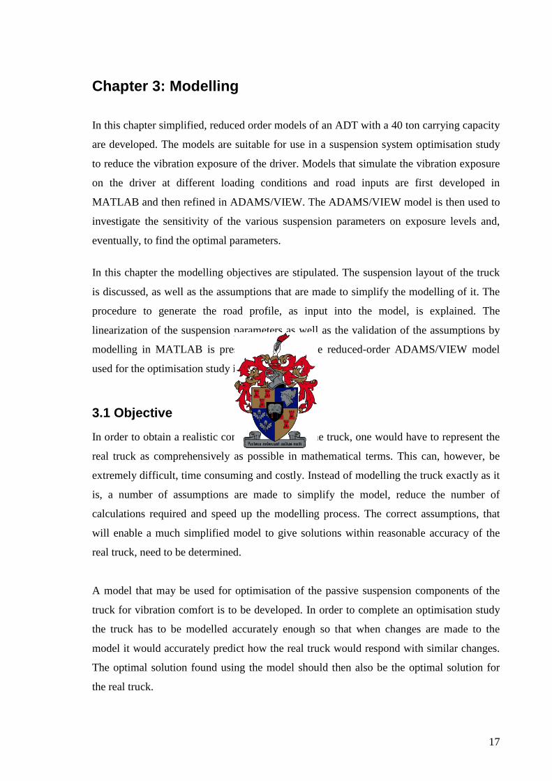
Figure 18: Axes, multipliers and weighting filters (Rimell, 2004)......................................39
Figure 19: Objective function representing switching of the worst-axis.............................43
Figure 20: Influence of variables of unloaded truck on RMS .............................................48
Figure 21: Influence of variables of unloaded truck on VDV .............................................49
Figure 22: Influence of variables of loaded truck on RMS .................................................50
Figure 23: Influence of variables of loaded truck on VDV .................................................51
Figure 24: Influence of variables of combined cycle on RMS............................................52
Figure 25: Influence of variables of combined cycle on VDV............................................53
Figure 26: Averaged, weighted RMS values per cycle element – Construction Site..........71
Figure 27: Weighted VDV values per cycle element – Construction Site ..........................72
Figure 28: Average, weighted RMS values per cycle element - Quarry .............................74
Figure 29: Weighted VDV values per cycle element - Quarry............................................74
Figure 30: Roadway profile for isolation of beaming (Margolis, 2001) .............................81

vii
Figure 31: First 2D MATLAB model..................................................................................83
Figure 32: Second 2D MATLAB model .............................................................................84
Figure 33: 3D MATLAB model - a) Side view, b) Front view ...........................................84
Figure 34: Chassis beaming simplification..........................................................................86

viii
List of Tables
Table 1: Values of Su(κo) for Spectral Density Functions ...................................................22
Table 2: Linearized Parameters of Suspension Components...............................................26
Table 3: Degrees-of-freedom of MATLAB models ............................................................27
Table 4: RMS and VDV values for MATLAB models .......................................................28
Table 5: Effect% of design variables on response...............................................................47
Table 6: Unloaded optimal suspension parameters for RMS exposure...............................54
Table 7: Unloaded optimal suspension parameters for VDV exposure...............................54
Table 8: Loaded optimal suspension parameters for RMS exposure ..................................55
Table 9: Loaded optimal suspension parameters for VDV exposure ..................................55
Table 10: Combined optimal suspension parameters for RMS exposure............................56
Table 11: Combined optimal suspension parameters for VDV exposure ...........................56
Table 12: % Improvement with optimal parameters on different road surfaces .................58
Table 13: WBV exposure as calculated by HSE calculator for construction site................79
Table 14: WBV exposure as calculated by HSE calculator for quarry................................79
Table 15: Degrees-of-freedom of MATLAB models ..........................................................85
ix
Glossary
2D Two Dimensional
3D Three Dimensional
A(8) Equivalent eight-hour RMS exposure
ADAMS∗ Automatic Dynamic Analysis of Mechanical Systems
ADAMS/CAR* Specialised environment in ADAMS for modelling vehicles
ADAMS/INSIGHT* Specialised environment in ADAMS for design-of-experiments
ADAMS/VIEW * Basic environment in ADAMS for simulating models
ADT Articulated Dump Truck
BFGS Broyden, Fletcher, Goldfarb and Shanno
CCD Central Composite Design
DADS* Dynamic Analysis Design Systems
DIRECT Divided Rectangle
DOF Degrees-of-Freedom
EAV Exposure Action Value
ELV Exposure Limit Value
EU European Union
eVDV Estimated Vibration Dose Value
FFT Fast Fourier Transform
F-Tire Flexible Ring Tire Model
GA Genetic Algorithm
GENRIT A general vehicle model for simulation of ride dynamics
GRG General Reduced Gradient
HSE Health and Safety Executive
ISO International Organisation for Standardisation
MATLAB * Matrix Laboratory
PAVD Physical Agents Vibration Directive
PSD Power Spectral Density
QP Quadratic Programming
RMS Root Mean Square
RSM Response Surface Methodology
∗ Commercially available Software

x
SQP Sequential Quadratic Programming
SWIFT Short Wavelength Intermediate Frequency Tire
VDV Vibration Dose Value
WBV Whole-Body Vibration
Wd ISO frequency weighting filter used for lateral and longitudinal
vibrations of seated human
Wk ISO frequency weighting filter used for vertical vibrations of seated
human

1
Chapter 1: Introduction
Drivers of Articulated Dump Trucks (ADTs) are exposed to vibration on a daily basis. In
the past, the South African industry has paid little attention to the measurement and control
of whole-body vibration, but new legislation introduced in Europe is encouraging that to
change. The levels of vibration induced in the drivers have the potential to compromise
occupational health and safety and are fast becoming a major concern in Europe; and in
South Africa for exporting manufacturers. In this project the passive suspension systems of
an ADT are optimised to reduce vibration exposure of the driver.
1.1 The Articulated Dump Truck
Articulated Dump Trucks are used in the mining and construction industries to efficiently
transport material (usually earth) over irregular terrain. The “articulation” refers to the
steering mechanism of the truck, which allows the front section to yaw independently of
the rear by means of hydraulic rams. ADTs usually operate on a large variety of road
surfaces ranging from very poor to well maintained dirt (or tar) roads. An ADT has various
suspension systems that isolate the driver from the inputs at the wheel/road interface, the
engine and other sources of noise and vibration. These include the tires, the primary
suspension, the cabin suspension and the seat suspension.
The tires have a larger travel than any other suspension system and thus play an important
role in isolating the driver from road irregularities. The primary suspension maintains
contact of tires and road surface and improves the handling and carrying capacity of the
truck. The cabin suspension (rubber mounts) and the seat suspension (air spring) isolates
the driver from vibrations transmitted from the engine, drive-train or road.
The typical loading cycle of an ADT (in the mining and construction industries) comprises
the following elements:
1. Moving across the quarry floor into the loading position (empty)
2. Loading (load dropped into the bin)
3. Moving across the quarry floor to the access road (fully laden)
4. Driving to the drop zone (fully laden)

2
5. Positioning in the drop zone
6. Tipping the load
7. Driving back to the quarry (empty)
The exposure levels vary from one cycle element to the next with the highest exposure
levels being recorded while the truck is driving fastest (cycle elements 4 and 7) and the
lowest exposure levels while loading or unloading (cycle elements 2 and 6). Drivers may
be expected to work up to 12 hour shifts, depending on the environment and type of load
(reviewed in appendix A).
1.2 Motivation
Until recently no legislation governing vibration exposure limits existed, but general
legislation required designers to do what is reasonably possible to reduce the health risks
associated with whole body vibration (WBV) exposure. The suspension systems were
designed to what was considered to be “reasonable” vibration exposure levels, focusing
more on handling and load carrying capacity. Studies have shown that in certain cases
suspension systems amplified the vibrations between 0-20Hz by as much as 4 times and as
many as 45% of seats used in industry increase rather than decrease the accelerations,
mainly due to end-stop impacts (Deprez et al., 2004). Current research on the health risks
of vibration exposure has led to a revision of legislation and the development of a Physical
Agents Vibration Directive (PAVD) by the European Union (Directive 2002/44/EC).
Included in this directive is an exposure action value (EAV) which determines what an
acceptable level of exposure is and an exposure limit value (ELV), which may not be
exceeded. The directive will be fully operational in Europe by 2010 (Brereton et al., 2004).
Manufacturers that export vehicles or other equipment to Europe will have to adhere to the
new legislation requirements to remain competitive. A vehicle that produces a high
vibration exposure on the driver may be required to stop before the end of a shift (when the
ELV is reached), while a competing manufacturer’s vehicle with lower vibration levels,
may be allowed to continue. This not only decreases productivity, but also damages the
image of the manufacturer whose vehicle had to stop. The European legislation may also
be used in South African courts as the benchmark to “state-of-the-art” technology.

3
Research has shown that human response to whole body vibration can cause discomfort,
interference with activities, impaired health, perception of low magnitude vibration and the
occurrence of motion sickness (Griffin, 1990). The results of this in the short term are
fatigue, loss of concentration and alertness (van Niekerk et al., 1998) and can eventually
lead to lower-back pain and musco-skeletal disorders. Drivers that are exposed to high
levels of vibration are more likely to make mistakes and cause damage to themselves, the
environment and the equipment they work with. A reduction in the exposure levels of the
driver may well lead to a reduction in medical and maintenance costs for the employee.
Lower back pain is the leading cause of industrial disability in those younger than 45 years
and accounts for 20% of all work injuries. The total cost a year in the US is estimated at
$90 billion (Deprez et al., 2004). These disorders are mainly caused by vibration between
0.5Hz and 80Hz, while motion at frequencies below 0.5Hz induces motion sickness (ISO
2631, 1997).
The manufacturer developed a complex 50 degree-of-freedom ADAMS/CAR model of the
truck to be used in predictive modelling. The model took a long time to develop and was
still not fully operational by the onset of the project. The suspension parameters (tested by
and independent institution) were available and would not have to be determined
experimentally. The tire stiffness and damping characteristics were obtainable from the tire
manufacturer.
1.3 Objectives for the Project
A simplified, reduced order model of an ADT with a 40 ton carrying capacity that is
suitable for use in a suspension system optimisation study to reduce the vibration exposure
of the driver was developed. The model can:
• Accurately simulate the vibration exposure of the driver.
• Be used to investigate the sensitivity of the various suspension parameters on
exposure levels.
• Simulate different loading conditions and road inputs.
In order to reduce the vibration level that a driver is exposed to, one needs to optimise the
total transmissibility between the various inputs and the driver on the seat within some
given constraints, such as the load the vehicle needs to carry, the vehicle dynamics, the

4
existing layout and available space. An objective of the project was to show that significant
reduction in vibration exposure levels may be achieved without changing the operation,
layout or physical dimensions of the current suspension systems or by reducing the load
carrying capacity of the vehicle.
Another objective was to determine the parameters of the current passive suspension
systems with the largest influence on the vibration exposure levels. These parameters were
optimised to produce the lowest exposure levels for a typical haul road. The stiffness and
damping characteristics of the various suspension systems were combined into a single
parameter for the optimisation study.
1.4 Thesis Overview
The motivation and objectives of the project were presented in this chapter. Chapter 2
focuses on the literature review. Suspension systems, vehicle dynamic models,
optimisation techniques and the legislation being introduced in Europe are discussed.
Chapter 3 deals with the modelling of the truck, the road inputs and general assumptions
used to simplify the model. Chapter 4 discusses how whole-body vibration exposure on
humans should be evaluated.
Chapter 5 focuses on objective functions and optimisation algorithms. Chapter 6 discusses
the importance of the various parameters, the optimisation results and includes the
verification of the results. The conclusions and recommendations are presented in Chapter
7.

5
Chapter 2: Literature Study
In the literature study the primary functions of the suspension systems and their
contribution to comfort are discussed. Various methods and the associated assumptions to
model the vehicle, road inputs and human dynamics are discussed. A dynamic simulation
software package is reviewed in this chapter. Whole-body vibration and the incorporation
of the newly developed legislation in Europe are presented. Finally optimisation techniques
from literature are investigated and discussed.
2.1 Primary Function of Vehicle Suspension
According to Gillespie (1992), the primary functions of a vehicle suspension are to:
• Provide vertical compliance so the wheels can follow the uneven road, isolating the
chassis from roughness in the road,
• Maintain the wheels in the proper steer and camber attitudes to the road surface,
• React to control forces produced by the tires,
• Resist roll of the chassis, and
• Keep the tires in contact with the road with minimal load variations.
A vehicle such as an ADT may have more than one suspension system. Each suspension
system performs a different function. The tires of the ADT are softer (and have more
travel) than the primary suspension and thus make a very large contribution to the isolation
of the vehicle from the road irregularities. The primary suspension’s (between wheels and
chassis) main function is vehicle dynamics and load carrying capacity and not so much
comfort. It serves to keep the wheels in contact with the ground and to prevent excessive
body roll. The cabin suspension’s (between chassis and cabin) and seat suspension’s
(between cabin floor and seat) main purpose is vibration isolation and thus contribute
toward the comfort of the driver.
In general, an improvement of vehicle suspension (systems) could produce the following:
• Improvement of vehicle ride quality,
• Increased mobility, and
• Increased component life.

6
This study will focus on improving the vehicle ride comfort in order to reduce WBV
exposure.
Cebon and Cole (1992) reported that, of all the types of suspensions generally used in
heavy vehicles, the walking beam and pivoted spring tandem suspensions (such as is used
in the ADT under investigation) generate the highest loads, leaf spring suspensions
generate less, and air and torsion bar suspensions generate the smallest level of dynamic
loads. Higher loads usually lead to the road surface being damaged quicker, which in turn
leads to a more irregular road that will include higher vibrations. The maintenance of the
road thus plays a vital role in reducing the vibration exposure levels on the driver.
2.2 Vehicle Dynamic Models
A reliable simulation model must include the vehicle (modelled as rigid or flexible bodies),
the human on a seat and road profile input. Most of the problems associated with the
safety, economy and overall quality of road transportation are affected by the
characteristics of the roads and the dynamics of the vehicles and the manner in which they
interact (Kulakowski, 1994).
Verheul (1994) suggested that a simplified truck model could be used as a prototype for a
more complex model. The simplest vehicle ride model is the 2-DOF (degree-of-freedom)
quarter car model. This model is useful to help understand basic concepts of suspension
properties and vehicle vibrations (Jiang, Streit, El-Gindy, 2001), but Gillespie and
Karamihas (2000) reported that because of the diverse properties of trucks, there is no
sound basis for selecting a single model representative of the “average” truck. The attempts
to generate a generic quarter-truck model were not very successful with results varying up
to 20% with comprehensive, non-linear truck models.
Two- and/or three-dimensional models may be developed to model the ride of a truck. A
number of models were investigated by El Madany and Dokainish (1980) and Cebon,
(1999). Agreement between 2D (two-dimensional) and 3D (three-dimensional) models are
usually good in the region of the sprung mass modes and where roll modes are not
significantly excited. It was concluded that where pitch and single plane vibrations
dominated, the two-dimensional model was adequate for ride studies. Fu and Cebon

7
(2002), in their analysis of truck suspension database, concluded that 2-DOF models are
adequate to compare suspensions with one another.
Some of the 2D and 3D models that have been developed to model trucks were researched
by Jiang, Streit and El-Gindy (2001). In their study they found that linear components
could give reasonable results (Wang and Hu, 1998), tandem suspensions could be
modelled as massless beams (Cole et al., 1992) and the road could be modelled from a
power spectral density distribution (Zhou, 1998). These simplifications would be
implemented in developing the optimisation model.
Ibrahim et al. (1994) developed a model to investigate the effect of a flexible frame on ride
vibration in large trucks. He concluded that frame flexibility may contribute significantly
to vibration measurements, especially on the trailer. In his article Donald Margolis (2001)
stated that the rigid body modes of a truck are most important at frequencies below 5Hz,
while beaming (transverse vibration of chassis) occurs close to the wheel-hop frequency at
about 10Hz. Beaming is difficult to control from the suspension locations, as the shock
absorbers do little to extract energy from the beaming mode. The primary suspension can,
however, be used to control the rigid body modes. If beaming is excited, it could be dealt
with through cab isolation techniques. A beaming investigation of the ADT (included in
Appendix D) showed that it may be ignored for the purposes of this project.
Most tire models are better suited to either ride or handling simulations and few models
can simulate both accurately. Two of the models that claim to be accurate enough to be
used for either simulation are the SWIFT (Short Wavelength Intermediate Frequency Tire)
and F-Tire (Flexible Ring Tire Model). Some of the models (in order of increasing
complexity, showed in Figure 1) that can simulate the enveloping properties of tires on
uneven roads, and are thus well suited to ride-models are (Zegelaar, 1998):
• single-point contact model (spring and damper in parallel),
• roller contact model (rigid wheel with one spring, one damper and a single contact
point),
• fixed footprint model (linearly distributed stiffness and damping in the contact
area),

8
• radial spring model (circumferentially distributed independent linear spring
elements),
• flexible ring model
• finite elements models.
Figure 1: Tire models suitable for Ride Simulations (Zegelaar, 1998)
Prasad (1995) stated in his article that it is widely accepted that poor tire description is the
main error in vibration prediction. Most researchers use Voigt-Kelvin (linear spring and
viscous damper in parallel) to simulate the tire behaviour. Usually characteristics of the
stationary tires are used although they may differ significantly from rolling tires. Kising
and Gohlich (1988), and Lines and Murphy (1991) showed that the Voigt-Kelvin
representation is a suitable representation of the radial characteristics of the tire. The
Voigt-Kelvin, roller contact model as shown in Figure 1, was implemented.
In modelling the human, one may choose between many different models. Biodynamic
models were obtained from the superposition of bio-dynamic responses from different
individuals. Most current models are little more than convenient simple mechanical
systems, the parameters of which have been adjusted to fit average transmissibility
(vibration through body) or impedance (transmission of vibration to the body) data.
Ideally, models should take into account the bending motions of the spine, the effects of
body posture, the non-vertical motions of the head, the effect of non-vertical seat vibration,
the effects of the backrest and the variation in motion at different points on the head.
Models of the impedance of the body should allow for variations in the static mass of the
body and the non-linearity evident with changing magnitudes of vibration (Griffin, 1990).
These models, however, will have many degrees of freedom. The more degrees of
freedom, the more accurate the model could be, but for optimisation studies a simplified
model would be adequate. ISO 7962 of 1987 prescribes a four degree-of-freedom

9
transmissibility model. For the optimisation study an impedance model would be better
suited. ISO 5982 of 1981 prescribes a three degree-of-freedom vertical-impedance model,
but a simple lumped parameter model was developed by Fairly and Griffin in 1989 that
gives satisfactory results up to 20Hz. It was decided to use the simple lumped parameter
model since it has the least degrees of freedom yet still gives acceptable accuracy up to
20Hz. Prasad (1995) and Verma and Gouw (1990) also developed similar models to Fairly
and Griffin (1989) with acceptable results, even incorporating non-linear effects such as
end-stops.
2.3 ADAMS
ADAMS (Automatic Dynamic Analysis of Mechanical Systems) is commercially available
multi-body system analysis software. It is the most widely used software package of its
kind. Modelling elements are the basic building blocks of dynamics, i.e. forces, bodies,
joints. By selecting and combining these elements, the user can build a dynamic model to
the required level of detail.
Once the model is defined, the user can request static, quasi-static, linear, kinematic,
dynamic or inverse-dynamic analysis of the system. ADAMS automatically formulates the
equations of motion and solves them in the time domain. It can even handle non-linearities
and impacts quite well.
ADAMS solves the equations of motion using a variable order and time step predictor-
corrector integration technique. The user sets the upper limit for time steps, but ADAMS
may use smaller time steps if it is necessary for achieving required accuracy or in the case
of sudden change in equations. ADAMS predicts the solution one step forward in time and
then corrects it with iteration. If the step is successful the next step is taken; otherwise, the
step is rejected and a smaller time step is tried. For more information see the
MSC.ADAMS Product Catalog (2002). It was decided to use ADAMS as the platform for
the optimisation model.

10
2.4 Whole Body Vibration
Whole body vibration is the mechanical vibration (or shock) transmitted to the body as a
whole. It is often due to the vibration of a surface supporting the body (Griffin, 1990). The
effects of vibration could be subdivided into three main headings, namely (a) interference
with comfort, (b) interference with activities and (c) interference with health. Each
criterion has different considerations and limits associated with it. Not all vibrations,
however, are bad and need to be avoided, for example shaking of hands or rocking in a
chair. Vibrations may provide feedback to warn of impeding failures and is used for
therapy or diagnostics in the medical field.
Vibration produces many different types of sensations as the frequency is increased and the
acceptability of the motion varies, but does not fall as rapidly as the decrease in vibration
displacement with increasing frequency (for a constant acceleration RMS magnitude). The
magnitude of vibration displacement which is visible to the eye of an observer therefore
gives a very poor indication of the severity of the vibration.
Frequencies below about 0.5Hz may eventually lead to symptoms of motion sickness
(most sensitive between 0.1Hz and 0.125Hz.). Different parts of the body resonate at
different frequencies. In the vertical direction resonance starts at about 2Hz, but the first
major resonance occurs at about 5Hz. The transmissibility of vertical vibration to the head
is sometimes a maximum at 4Hz and the driving force per unit acceleration (as well as the
discomfort) is a maximum at about 5Hz. The voice may be caused to warble by vibrations
between 10Hz and 20Hz. Vision may be affected at any frequency, but blurring occurs
between 15Hz and 60Hz. The dominant vibration transmitted through the seats of vehicles
is often at frequencies below 20Hz (Griffin, 1990). It was thus decided to limit the
investigation to frequencies below 20Hz.
Comfort is a more difficult to determine since it is subjective and has a lot to do with the
psyche. It is important to note that frequency and not only amplitude contribute to the
perception of comfort. An experiment done by Fothergill and Griffin in 1977 showed that
for a seated person excited by a 10Hz sinusoidal vibration for RMS values below 0.4m/s2
it was noticeable, but not uncomfortable. A level of 1.1m/s2 was considered to be mildly

11
uncomfortable, 1.8m/s2 uncomfortable and RMS values above 2.7m/s2 as very
uncomfortable.
Most researchers agree that seated humans have a vertical vibration natural frequency at
about 4 - 6Hz and a horizontal vibration natural frequency at about 1 – 2Hz. In these
frequency ranges the seat motion is most easily transmitted to the upper parts of the body
and is not just confined to the area of the body close to the source of vibration. Both Huang
and Ji (2004) reported a decrease in natural frequency as the magnitude of the excitation
frequency is increased. The resonance of humans decrease from 6 to 4Hz as the magnitude
of vibration is increased from 0.25 – 2m/s2 (Ji, 2004).
The human body’s vibration characteristics are non-linear. In his article, Huang (2004)
stated that some of the factors that cause non-linearity of apparent mass of a human are
posture, muscle tone, dynamics of the buttocks tissue and body geometry. The muscle tone
probably made the biggest contribution to non-linearity of the human body’s apparent
mass.
Research on the effect of posture of a person on natural frequency showed that when the
feet of a seated human are not supported (i.e. the feet are hanging) two natural frequencies
are witnessed (one between 1-2Hz and the other at around 5Hz), but when the feet of the
person are supported only one natural frequency is witnessed (Nawayseh, 2004). Also,
when holding a steering wheel, the resonance at 4Hz is more pronounced than when the
hands are on the lap (Toward, 2004). A driver usually is excited more than the passenger
because of this phenomenon.
Impedance measurements in the horizontal axes show resonances at around 1-2Hz when
there is no backrest. A backrest has an effect on fore-aft axis, but little effect on the other
axes (Griffin, 1990).
2.5 Legislation
The European Union Directive 2002/44/EC (known as the Physical Agents Vibration
Directive or PAVD) set out the minimum standards to be achieved by Member States for

12
the protection of workers from vibration injury. The PAVD applies the principles of risk
management to prevent risks presented by exposure to vibration.
The EU-Directive prohibits the exposure above the exposure limit value (ELV) of 1.15m/s2
RMS for 8 hours (or 21m/s1.75 VDV). If the exposure exceeds an exposure action value
(EAV) of 0.5m/s2 RMS (or 9.1m/s1.75 VDV) a programme of continual improvement
should be implemented by the employer. Whether RMS (root mean squared) or VDV
(vibration dose value) should be used is at the choice of the Member State concerned (EU-
Directive, 2002).
WBV exposures are to be determined separately for the three axes in accordance with ISO
2631-1:1997 and for health surveillance the axes with the highest level of vibration will be
used. The EU-directive is to be implemented on the 6th July 2005 with a transitional period
of 5 years for equipment issued before 6th July 2007. The EU-Directive is to be revised
every 5 years (EU-Directive, 2002).
In managing the risk of exposure to vibration, exposure should be reduced, but only so far
as is reasonably practical. It would be fair to assume that most operators of machinery used
off-road are exposed above the EAV. A few processes will cause exposures above the ELV
and these should become well known over the next few months as guidance is published.
In short, employers should ask themselves: What is good practice? And is good practice
being followed? (Brereton, 2004).
At present the EU-Directive and ISO 2631-1:1997 stipulates what the requirements and
standards of WBV exposure and measurement are. These documents don’t account for all
possible situations and consequently a couple of questions (such as what equipment should
be used to measure accelerations) were raised about the measurement and evaluation of
WBV on humans. A study done by Darlington (2004) on different measuring instruments
showed that certain instruments claiming to conform to international standards, that were
correctly calibrated and used within their intended operating envelope returned results
differing by as much as 30%.
Gallais (2004) found that comfort is time dependent and suggested that time dependency
filters should be incorporated in the evaluation of WBV. ISO 2631 of 1997 does not

13
compensate for time dependency of comfort. It was noted that such dependency curves
were included in the ISO of 1974, but was since removed.
Up to date there has been much debate about whether the energy equivalent acceleration
A(8) or the VDV measurements should be used to evaluate WBV on seated humans. The
arguments for and against the VDV measurements are usually that it is better at indicating
the presence of peaks (which tend to be more harmful to humans), but is also more
sensitive to human induced motions such as shuffling. Research done by Newell (2004)
showed that an operator could exceed the vibration dose action value of the Physical
Agents Vibration Directive (9.1m/s1.75) by artefacts such as ingress and egress alone with
no “authentic” WBV exposure. If it were important that ingress and egress should form
part of the daily WBV measurements, then office workers should also be included in the
Directive. Tests done on a wheel loader showed that getting in and out of the loader 6
times per day would be enough to exceed the EAV.
2.6 Suspension Optimisation
From Naudè (2001) we see that: Suspension optimisation is the process through which
decisions are made on the specific choices of characteristics for the suspension components
such that certain prescribed design objectives or evaluation criteria are fulfilled. These
criteria may be the attainment of a certain level of ride-comfort over specified terrain and
vehicle speed.
Basic approximation vehicle models are used to test the assumptions that simplify the
modelling of the specific vehicle. The initial basic approximation models usually assume
linear characteristics for suspension components such as the springs and dampers. The
second step is to perform a more extensive and detailed analysis of the vehicle concerned.
This can be done by performing vehicle simulations using vehicle dynamic simulation
programs such as, for example, DADS (Dynamic Analyses Design Systems) or ADAMS.
In these more advanced programs the suspension components could have linear or non-
linear characteristics. Once the model is validated, the vehicle dynamics may be evaluated
over different specified routes and speeds. By changing the suspension characteristics,
their influence on the vehicle dynamics may be assessed.

14
There are many examples of optimisation studies from literature. Heyns (1992) optimised
the suspension of a container carrier for ride comfort using GENRIT software. Heui-bon
Lee et al. (1997) optimised the suspension of a medium truck for ride comfort using road
inputs from PSD (Power Spectral Density) plots and DADS software. Motoyama (2000)
used a genetic algorithm to optimise the 18 design variables to minimise suspension toe
angle. The optimal solution was obtained from a response surface. Lee et al. (2000)
optimised a train’s bogie suspension using fuzzy logic and Vampire software. The 26
design variables were optimised with the help of a response surface. The procedures used
in the above examples would also be applied to the current optimisation study.
As can be seen from the abovementioned examples, as well as other investigations reported
in literature, optimisation and analysis of a vehicle suspension can be complex, expensive
and time consuming. These factors force the design engineer to take a more pragmatic
approach summarised by the statement of Esat (1996): “The important goal of optimisation
is improvement and attainment of the optimum is much less important for complex
systems”.
Due to the fact that the suspension characteristics in semi-active or active suspensions can
be changed according to the terrain requirements, these types of suspension systems can
improve ride quality over a wide spectrum of terrain. These improvements come at the
penalty of increased complexity and higher cost. A large amount of research has been done
on control algorithms for such suspension systems.
Due to the associated higher cost and increased complexity, semi-active and active
suspension systems are still relatively rare. This study will be limited to the optimisation of
passive suspension systems.
2.7 Optimisation Algorithm
Engineers use models to predict a response or a dependent variable, given the values of
other characteristics, called independent variables (regressors or predictors). Engineers
require data to estimate these models. The method of least squares estimates the parameters
of the model by minimizing the errors between predicted and observed data. SStotal, the
variability in the data, can be partitioned into two components: SSreg, which represents the

15
variability explained by the regression model, and SSres, which measures the variability left
unexplained and usually attributed to error. The coefficient of determination, R2, uses the
relative sizes of the variability explained by the regression model and the total variability
to measure the overall adequacy of the model (Vining, 1998). It is defined by:
total
res
SS
SSR −= 12 , ( 1 )
this guarantees that 0 ≤ R2 ≤ 1. R2 may be interpreted as the proportion of the total
variability explained by the regression model. For the purposes of optimisation, an R2 value
of 0.9 (that is, 90% of the variability is described by the regression model) is acceptable
(ADAMS/INSIGHT help file, 2004).
The response surface methodology (RSM) is a method to generate a regression model and
uses a sequential philosophy of experimentation. To estimate a second-order model the
design must have at least as many distinct treatment combinations as terms to estimate in
the model and each factor must have at least three levels. The most common used design to
estimate the second order model is the Central Composite Design (CCD). There are
different CCD’s that uses different values for α. Typical choices for α are:
• 1, creating a face-centred cube CCD,
• k0.5, creating a spherical CCD
• nf0.25, creating a rotatable CCD, where nf is the number of factorial runs used in the
design.
Figure 2: Three-Factor Central Composite Design (Vining, 1998)

16
For k factors, the full factorial design consists of every possible combination of the three
levels (upper, lower and centre) for the k factors, giving 3k combinations. The regression
model may then serve as the objective function for an optimisation study (Vining, 1998).
Several classes of optimisation algorithms have been developed. The most important
classes are (Naudè, 2001):
• Mathematical programming methods (including gradient based methods such as,
for example, Sequential Quadratic Programming)
• Lipschitzian and deterministic optimisation and
• Genetic algorithms (GAs)
For the purposes of this project a single Lipschitzian based algorithm (DIRECT) is
implemented. The DIRECT algorithm is more robust in determining the approximate
coordinates of the global minimum than the gradient based methods. The gradient based
algorithms are more efficient in determining the coordinates of local minima (which may
or may not include the global minimum). Three gradient based algorithms are used to
determine the optimal solution. The solution is then correlated with the DIRECT
algorithm’s solution to ensure that it is indeed a global minimum. The algorithms are
discussed in Chapter 6.
In this chapter it was shown that the suspension could be optimised to improve the ride
quality. The assumptions that could reduce the complexity of the truck model were
presented. It was seen that only frequencies below 20Hz are important for this study and
that VDV or RMS measures may be used to judge the severity of a vibration exposure
level. Examples from literature showed that the response surface methodology is a feasible
optimisation technique for a study such as this. The regression model and procedure
required to generate a response surface was presented. Finally the optimisation strategy
was presented.
17
Chapter 3: Modelling
In this chapter simplified, reduced order models of an ADT with a 40 ton carrying capacity
are developed. The models are suitable for use in a suspension system optimisation study
to reduce the vibration exposure of the driver. Models that simulate the vibration exposure
on the driver at different loading conditions and road inputs are first developed in
MATLAB and then refined in ADAMS/VIEW. The ADAMS/VIEW model is then used to
investigate the sensitivity of the various suspension parameters on exposure levels and,
eventually, to find the optimal parameters.
In this chapter the modelling objectives are stipulated. The suspension layout of the truck
is discussed, as well as the assumptions that are made to simplify the modelling of it. The
procedure to generate the road profile, as input into the model, is explained. The
linearization of the suspension parameters as well as the validation of the assumptions by
modelling in MATLAB is presented. Finally, the reduced-order ADAMS/VIEW model
used for the optimisation study is reviewed.
3.1 Objective
In order to obtain a realistic computer model of the truck, one would have to represent the
real truck as comprehensively as possible in mathematical terms. This can, however, be
extremely difficult, time consuming and costly. Instead of modelling the truck exactly as it
is, a number of assumptions are made to simplify the model, reduce the number of
calculations required and speed up the modelling process. The correct assumptions, that
will enable a much simplified model to give solutions within reasonable accuracy of the
real truck, need to be determined.
A model that may be used for optimisation of the passive suspension components of the
truck for vibration comfort is to be developed. In order to complete an optimisation study
the truck has to be modelled accurately enough so that when changes are made to the
model it would accurately predict how the real truck would respond with similar changes.
The optimal solution found using the model should then also be the optimal solution for
the real truck.

18
A 50 degree-of-freedom ADAMS/CAR model of the 40 ton ADT was developed by the
manufacturer. For this optimisation study, a simplified model with fewer degrees-of-
freedom than the one that already exists is to be developed. The model should also be
simulated under different loading conditions and on different road surfaces. The influence
of the various suspension parameters on the vibration exposure should be suitably
simulated by the model.
3.2 Vehicle Characteristics
It is important to understand how each suspension component functions before it may be
simplified. The different suspension components will be discussed next according to Grovè
(2003):
The front suspension consists of the A-frame structure (also called banjo housing), the
front suspension struts and the cross-link (pan-hard). The A-frame is connected to the
front chassis via a flexible pivot mount. The suspension struts are connected to the A-
frame and the front chassis via flexible spherical mounts (sphericals). The cross link is
connected to the A-frame structure and the front chassis with the same sphericals as for the
suspension struts. The front suspension struts are filled with a combination oil and nitrogen
under high pressure. The nitrogen provides the required “spring” characteristics while the
hydraulic oil provides the required “damping” characteristics. On both ends of the strut,
sphericals are used to connect the struts to the front chassis at the top and the A-Frame
structure at the bottom. Figure 3 shows the front suspension without the front chassis:
Figure 3: Front Suspension (Grovè, 2003)
Strut
Spherical Joint
Cross Link
A-Frame Pivot
A-Frame

19
The rear suspension is more complex than the front suspension. The mid and rear axle
housings are connected to the walking beam via sandwich blocks. The walking beams are
connected to the rear chassis via flexible pivot mounts. All of the links (top drag, bottom
drag & cross) are connected to the axle housings and to the rear chassis via the same
flexible spherical mounts as on the front suspension. Figure 4 below shows the rear
suspension without the rear chassis:
Figure 4: Rear Suspension (Grovè, 2003)
The sandwich blocks are used as flexible elements between the walking beams and the mid
and rear axles. In Figure 4 and Figure 5 c) the sandwich blocks are seen in their attached
position in the rear suspension.
Walking Beam
Sandwich Block
Link Axle Housing
Pivot

20
(a) (b)
(c)
Figure 5: a) Sandwich block, b) Cab mount, c) Bin shock mats (Grovè, 2003)
Four cab mounts as shown in Figure 5 are used to mount the cab to the front chassis of the
vehicle. The bushings that form the cab suspension only isolate the cabin from high
frequency vibration caused by the engine and ancillary equipment.
The bin shock mats are used to provide a cushioned support for the bin on the rear chassis.
There are two sets (2 x 2) mats in the mid position and one set (1 x 2) at the front position.
The mats are in essence bump stops. The bin mats are shown in Figure 5 c).
The force versus displacement (static) and force versus velocity (dynamic) characteristics
for various components were experimentally determined. The components that were
measured are: A-Frame pivot, spherical, strut and link spherical, suspension stops, walking
beam pivot, sandwich blocks, cab mountings, bin shock mats, engine mountings, drop box
mountings and suspension strut. There was variability in the dynamic and static
characteristics of the components of up to 18% (van Tonder, 2003). The mass and inertia
of the structural components of the truck were supplied by the manufacturer.

21
To reduce the complexity of the model the following assumptions were made:
• All components that are to be optimised are modelled with linear characteristics.
• Only parts or assemblies with a mass of 200kg (about 0.7% of the empty truck) or
more is considered (except for the human and seat).
• Steering and drive-train are not included (except for mass and inertia properties).
• Tires are modelled as Voigt-Kelvin (spring damper) systems.
• Front suspension is modelled as a single (constrained) axle with struts.
• The human on the seat is modelled as a simple 2-DOF lumped parameter model.
• All structural components are considered to be rigid.
3.3 Road Profile
Road profiles fit the general category of “broad band random signals” and, hence, can be
described either by the profile itself or its statistical properties. One of the more useful
representations is the PSD function (Gillespie, 1992).
As any random signal, the elevation profile measured over a length of road can be
decomposed by a Fourier transformation into a series of sine waves varying in their
amplitudes and phase relationships. A plot of the amplitudes versus spatial frequency can
be represented as a PSD. Spatial frequency is expressed as the “wave-number” with units
of cycles/meter and is the inverse of the wavelength of the sine wave on which it is based.
The displacement spectral densities of different road classes (smooth highway, gravel road,
ploughed field) are recorded in literature (Wong, 1978, Gillespie, 1992 and Cebon, 1999).
It has been found that the relationship between spectral density and spatial frequency can
be approximated by (Cebon, 1999):
nuu SS −= ))(()(
00 κ
κκκ ( 2 )
where κ = wavenumber
κ0 = datum wavenumber, 1/(2π) cycles/m
Su(κ) = displacement spectral density, m3/cycle
Su(κo) = spectral density at κo, m3/cycle

22
Table 1: Values of Su(κo) for Spectral Density Functions
for Various Surfaces (Wong, 1987)
Description n Su(κo) in m3/cycle
Smooth runway 3.8 4.3 x 10⁻¹¹
Rough runway 2.1 8.1 x 10⁻⁶
Smooth highway 2.1 4.8 x 10⁻⁷
Highway with gravel 2.1 4.4 x 10⁻⁶
Pasture 1.6 3.0 x 10⁻⁴
Ploughed field 1.6 6.5 x 10⁻⁴
Typical spectral densities of road elevation profiles simply reflect the fact that deviations
in the road surface are larger when the wave-number is large, but decreases as the wave-
number is decreased.
Road roughness is the deviation in elevation as seen by the vehicle as it drives over the
road. The most meaningful measure of ride vibration is the acceleration produced. The
roughness should thus be viewed as an acceleration to understand the dynamics of the ride.
Two steps are involved. Firstly a speed must be assumed such that the elevation profile is
transformed to displacement as a function of time. Differentiating once gives velocity and
twice gives acceleration. The conversion from spatial frequency (cycles/meter) to temporal
frequency (cycles/second or Hz) is obtained by multiplying the wave-number by the
vehicle speed in meter/second.
Viewed as an acceleration input (Figure 6 c)), road roughness presents its largest inputs at
high frequency, and thus has the greatest potential to excite high-frequency ride vibrations
unless attenuated accordingly by the dynamic properties of the vehicle. At any given
temporal frequency the amplitude of the acceleration input will increase with the square of
the speed.

23
Figure 6: a) Elevation, b) velocity and c) acceleration PSDs of road roughness input (Gillespie, 1992)
The normalised roll input (roll/vertical) PSD (Figure 7) show that at low wave-numbers
(long wavelengths) the roll input is much less than the vertical input, but as wavelengths
become shorter the correspondence between left and right diminishes and the roll input
magnitude grows. The roll resonance is thus excited a lot more at low velocities than at
high velocities. This may explain why the lateral vibration exposure may exceed the
vertical vibration exposure at low speeds.
Figure 7: Spectral density of normalised roll input for typical road (Gillespie, 1992)
a) b) c)

24
A rigid tread band model from Ahmed and Goupillon (1997) was used to take into account
the spatial filtering of the ground profile by the tires. This model assumes a point contact
between the tire and the ground and, to determine the excitation path due to the unevenness
of the ground, the road profile p(x) was replaced by the path u(x) of the centre of the tire
tread band, which was assumed to be rigid. u(x) is expressed in terms of p(x) by the
following equation:
22 ')'()( xRxxpxu −++= ( 3 )
Figure 8: Rigid tread band model (Ahmed and Goupillon, 1997)
where R is the radius of the tire (undeformed) and x’ is such that the contact point S is at
x+x’ (with |x’|<R). x’ is determined by assuming the angle between the normal force
(which is parallel to the line SC joining the point of contact with the centre of the tire) and
the vertical is equal to the slope of the ground profile at the point of contact S.
3.4 Linearization
All the suspension components are usually non-linear. The object of linearization is to
derive a linear model whose response will agree closely with that of the non-linear model.
Although the responses of the linear and non-linear models will not agree exactly and may

25
differ significantly under some conditions, there will generally be a set of inputs and initial
conditions for which the agreement will be satisfactory. (Close et al., 2002)
Linearization is carried out about an operating point and there are different ways to
determine the linear curve that suits the problem. If the range about the operating point is
small, the gradient of the non-linear curve at the operating point is taken as the linearized
equivalent. This may be done by replacing all non-linear terms by the first two terms of
their Taylor series expansion and ignoring the higher order terms. If the range about the
operating point is larger it may be necessary to perform a curve fit using an optimisation
technique such as least squared, alternatively more than one operating point may be
considered.
In real life the truck’s suspension often collides with the top and bottom end-stops
indicating that the full range is used. For the unloaded truck the extension-stops are hit
more often, while for the loaded trucks the bump-stops are hit more often. The parameters
were linearized (using the least squares curve fitting technique) over the entire range
between bump/extension stops. Figure 9 shows the measured stiffness of two struts, a non-
linear approximation to the measured results as well as the linearized stiffness of the strut
over its operating range. The displacement is negative when the strut is elongated and
positive when compressed (as tested). The gradient of the curve is the stiffness of the strut,
while the y-axis intercept describes the preload (as tested). The procedure was repeated for
all the suspension components and the results are included in Table 2. The stiffness and
damping of the seat is taken from the lumped model developed by Fairly and Griffin
(1989).

26
y = 0.7x + 51.841
20
30
40
50
60
70
80
90
100
110
120
-35 -30 -25 -20 -15 -10 -5 0 5 10 15 20 25 30 35 40 45 50 55 60
Deflection [mm]
Str
ut F
orce
[kN
]
STRUT 1
STRUT 2
Theoretical
Linear(Theoretical)
Figure 9: Linearization of Strut Stiffness
Table 2: Linearized Parameters of Suspension Components
Suspension Component Linearized Parameters
(N/mm), (Ns/mm), (kNm/deg)
Unloaded Preload
kN
Loaded Preload
kN
Strut Stiffness 700 58.2 98.7
Strut Damping 17.1 - -
Front Tires Stiffness 1130 71.7 75
Front Tires Damping 15 - -
Rear Tires Stiffness 1250 34.9 100
Rear Tires Damping 19 - -
Cab mounts Stiffness 1157 2 2
Cab mounts Damping 1.22 -
Bin Shock Mats Stiffness 15000 99 157.5
Bin Shock Mats Damping 25.1 - -
Torsion Spring Stiffness 840.6 - -
Torsion Spring Damping 5.1 - -
Sandwich Blocks Stiffness 8000 31.2 84.8
Sandwich Blocks Damping 20 - -
Seat Stiffness 120 0 0
Seat Damping 3.23 - -

27
To check the validity of the assumptions and linearization of the suspension parameters,
three models of the ADT, each with increasing complexity, were developed and modelled
in MATLAB (see Table 3).
Table 3: Degrees-of-freedom of MATLAB models
2 Dimensional 4 degree-of-freedom model
2 Dimensional 7 degree-of-freedom model
3 Dimensional 15 degree-of-freedom model
Vertical displacement:
• Chassis • Walking beam
Angular displacement about
y-axis (pitch):
• Chassis • Walking beam
Vertical displacement:
• Chassis • Walking beam • Cabin • Bin
Angular displacement about
y-axis (pitch):
• Chassis • Walking beam • Cabin
Vertical displacement:
• Chassis • Two walking beams • Cabin • Bin • Seat
Angular displacement about
y-axis (pitch):
• Chassis • Two walking beams • Cabin • Bin
Angular displacement about
x-axis (roll):
• Front chassis • Rear chassis • Cabin • Bin
To assess their performance a spectral analysis was performed on the vibration signal from
each model and the signals were converted from the time domain to the frequency domain.
The idea being that if there is energy present at any frequency it will appear in the spectral
plot. The most useful technique for analysing the frequency content of the signals is the
PSD. It generates a measure of the energy contained within a frequency band and is
calculated from the FFT of the signal (Mansfield, 2005).
Each model was simulated as driving over a rough road and the results (indicated as
normalised PSDs in Figure 10) were compared to the measurements taken in a real truck.
The PSDs are normalised, because the exact road surface on which the truck measurements
were made is not known and the relative amplitudes at specific frequencies are more
important than the absolute amplitudes.

28
Initially a 2-dimensional, 4-DOF model of the truck was developed and simulated. The
model managed to capture the 2Hz peak on the floor in the z-direction (correlating with the
rigid body mode of the ADT). The 2-dimensional model was then extended to a 7-DOF
model and was again simulated in MATLAB. The 7-DOF model managed to capture the
second peak near 20Hz (correlating with the rear-suspension wheel-hop frequency) which
the 4-DOF model could not. Finally a 3-dimensional, 15-DOF model was developed and
simulated in MATLAB. The model had reasonable accuracy as may be seen in Figure 10.
Most of the peaks were obtained fairly accurately except for the lateral (Y) direction on the
seat. The MATLAB models are further discussed in Appendix C.
The exact profile of the road is not known. Modelling an incorrect road surface will
contribute to the discrepancy between measured and simulated results. Simulating the cross
correlation between left and right wheel inputs incorrectly would influence the lateral
direction the most. The MATLAB models did not simulate the non-linear end-stops and is
expected to produce lower vibration dose values than the real truck. The simulations also
assumed a constant speed, which is not possible in a real truck travelling over irregular
terrain. The longitudinal direction would be influenced most by this assumption. The VDV
and RMS values for the MATLAB models and measured results are recorded in Table 4.
Table 4: RMS and VDV values for MATLAB models
Seat X Seat Y Seat Z Floor Z
Measured 0.34 0.86 0.58 0.55
3-dimensional 15-DOF model 0.23 0.81 0.51 0.55
2-dimensional 7-DOF model - - - 0.39
2-dimensional 4-DOF model
RMS (m/s2)
- - - 0.31
Measured 0.96 2.37 1.67 1.54
3-dimensional 15-DOF model 0.26 1.87 1.31 1.34
2-dimensional 7-DOF model - - - 1.5
2-dimensional 4-DOF model
VDV (m/s1.75)
- - - 0.76

29
Figure 10: Validation of MATLAB models
a)
b)
c)
d)

30
3.5 ADAMS/VIEW Model
In the previous section it was shown that the linearization of the suspension parameters and
the assumptions that were made gave reasonably good results. The end-stops were not
included in the MATLAB models, and the travel of certain suspension subsystems was
consequently exceeded. In order to optimise the parameters, the non-linear effects of the
end-stops had to be incorporated, especially when simulating very rough terrain as the
input. To simulate the truck even more accurately, a model was developed using
ADAMS/VIEW. The 24-DOF ride model that was developed in ADAMS/VIEW is shown
in Figure 11.
Figure 11: ADAMS/VIEW model of loaded truck
Since the truck does not have a drive-train or steering mechanism the truck was modelled
with each wheel positioned on top of a vertical actuator. The actuators move up and down
representing the surface of the road. The wheels are free to lift off the actuator when the
acceleration becomes too large. The human and seat was modelled as a lumped parameter
system. The bump and rebound stops were modelled as contact forces. If a certain
displacement is exceeded, spring and damper forces would increase exponentially, forcing
the body back into the operating range. The load is fixed to the bin and the bin can only
move vertically relatively to the rear chassis. None of the components are allowed to rotate
about the vertical (Z) axis. The degrees of freedom may be summarised as:
• vertical displacement of each wheel (6),
• angular displacement of the axles about the x-axis (3),
• vertical displacement of the axles (3),
• angular displacement of the walking beams about the y-axis (2),

31
• vertical displacement of the chassis (1),
• angular displacement of front and rear chassis about the x-axis (2),
• angular displacement of the chassis about the y-axis (1),
• vertical displacement of the cab (1)
• angular displacement of the cab about the x- and y-axis (2),
• vertical displacement of the load-bin (1),
• vertical displacement of the seat and the human (2).
3.6 Validation
A comprehensive ADAMS/CAR model of the ADT was developed by the manufacturer to
simulate the truck as accurately as possible. The ADAMS/CAR model is fairly complex,
having 50 degrees-of-freedom and non-linear suspension parameters. The tires were not
modelled as point contact Voigt-Kelvin (see Figure 1) as was the case with the
ADAMS/VIEW model, but instead the F-Tire developed by Michael Gipser (1999) was
used. The results obtained by the simplified model created in ADAMS/VIEW were
compared with results obtained by the ADAMS/CAR model as well as with measured
results from real trucks.
In order to validate the model it is important that the inputs into the model are the same as
the inputs experienced by the truck. It is very difficult to accurately describe a road’s
surface, thus it was decided to use an obstacle of known shape and size for verification
purposes. A cosine-shaped bump was constructed with a wavelength of 1.8m and a height
of 0.3m. The truck attempted to drive over the bump at approximately 8km/h, but the speed
of the truck did not remain at exactly 8km/h as it crossed the bump.
A comparison between the complex ADAMS/CAR model and a real truck had already
been done. These results served as the basis for validation of the newly developed,
ADAMS/VIEW model. To reproduce the inputs a spline of the displacement as a function
of time was generated. The displacements were then reproduced by the actuators at the
base of the wheels of the model.

32
Unfortunately no data was available for the cabin or seat, thus the comparisons had to be
based on strut and chassis data.
In Figure 12 the acceleration on the front chassis was recorded. In both graphs the dash-
dotted line represents the ADAMS/VIEW model while the solid lines represent the data
from the more complex model (top figure) and the measured data (bottom figure). In the
measured data a small bump is seen just after 2s, the ADAMS/VIEW model simulated the
bump, while the more complex model did not. Due to the linearization of the parameters
over the entire range (see Figure 9 on pg 26), one would expect the frequencies to
correspond well when large displacements are present (such as when crossing the bump),
but slightly inaccurate (over or under, depending on load condition) when displacements
are small. This explains why the results of the ADAMS/VIEW model oscillate slightly
faster than the other results when the amplitude decreases.
In Figure 13 the normalised PSDs of the acceleration data from Figure 12 is shown. It is
clear from the graphs that the frequency content of both ADAMS models are the same, but
their relative importance are not quite the same. The frequency of the main peak
corresponds well with what was measured in the real truck, but the other frequencies were
slightly too high, mainly due to the linearization and load condition of the truck (the
frequencies would shift slightly to the left for the loaded truck.)

33
0 2 4 6 8 10 12−15
−10
−5
0
5
10
15
20Front Chassis Acc − Model
m/s
2
time (s)
ADAMS/CARADAMS/VIEW
0 2 4 6 8 10 12−15
−10
−5
0
5
10
15Front Chassis Acc − Measurement 1
m/s
2
time (s)
MeasuredADAMS/VIEW
Figure 12: Validation - Front Chassis acceleration time history
0 1 2 3 4 5 6 7 8 9 100
0.2
0.4
0.6
0.8
1Front Chassis PSD/FFT − Model
Nor
mal
ised
Frequency (Hz)
ADAMS/CARADAMS/VIEW
0 1 2 3 4 5 6 7 8 9 100
0.2
0.4
0.6
0.8
1Front Chassis PSD/FFT − Measurement
Nor
mal
ised
Frequency (Hz)
MeasuredADAMS/VIEW
Figure 13: Validation - Front Chassis PSD

34
In Figure 14 the displacement of the strut is recorded as the truck traverses the bump. The
flat peaks are due to end-stop impacts. It is again clear that the ADAMS/VIEW model
follows the measured results more closely than the ADAMS/CAR model. Again the spike
at about 2s is missed by the ADAMS/CAR model, but simulated by the ADAMS/VIEW
model. The frequencies correspond fairly well over most of the data range, but become
slightly too high as the displacements decrease. The damping in the real truck also seems
to be higher than in either model.
0 2 4 6 8 10 12−40
−30
−20
−10
0
10
20
30
40
50Strut Displacement − Model
mm
time (s)
ADAMS/CARADAMS/VIEW
0 2 4 6 8 10 12−40
−30
−20
−10
0
10
20
30
40Strut Displacement − Measurement 1
mm
time (s)
MeasuredADAMS/VIEW
Figure 14: Validation - Strut displacement time history
In Figure 15 the normalised PSDs of the strut displacement data is shown. The
ADAMS/VIEW model seems to be a little closer to the real truck than the ADAMS/CAR
model. The minor peaks are slightly over-estimated as before.

35
0 1 2 3 4 5 6 7 8 9 100
0.2
0.4
0.6
0.8
1Strut Displacement PSD/FFT − Model
Nor
mal
ised
Frequency (Hz)
ADAMS/CARADAMS/VIEW
0 1 2 3 4 5 6 7 8 9 100
0.2
0.4
0.6
0.8
1Strut Displacement PSD/FFT − Measurement
Nor
mal
ised
Frequency (Hz)
MeasuredADAMS/VIEW
Figure 15: Validation - Strut Displacement PSD
A comparison between the newly developed ADAMS/VIEW model and the
manufacturer’s ADAMS/CAR model, on the randomly generated road surface that was
used for the optimisation study, is shown in Figure 16. The FFTs are calculated from
acceleration measurements taken on the cabin floor underneath the seat.
In the top graph of Figure 16 the FFTs of the longitudinal vibrations are recorded. The first
peak (corresponding to the rigid body pitching mode) compares well with the more
complex model. The two peaks that are generated by the ADAMS/CAR model close to
4Hz are not generated by the ADAMS/VIEW model. It is believed that these peaks are due
to input from the drive-train as the drive-train would have the largest influence on the
longitudinal vibration exposure. The drive-train was not simulated in the ADAMS/VIEW
model. It is, however, also possible that these peaks are overestimated by the
ADAMS/CAR model as was the case in Figure 13 and Figure 15 above.
In the middle and bottom graphs of Figure 16 the FFTs of the lateral and vertical vibrations
are recorded respectively. The ADAMS/VIEW model correlated well with the more

36
complex ADAMS/CAR model for both vibration axes even though it had less than half the
number of degrees-of-freedom.
0 2 4 6 8 10 12 14 16 18 200
0.02
0.04
0.06
0.08
Cabin Floor FFTX
Hz
m/s
2 /Hz
ADAMS/CARADAMS/VIEW
0 2 4 6 8 10 12 14 16 18 200
0.05
0.1
Cabin Floor FFTY
Hz
m/s
2 /Hz ADAMS/CAR
ADAMS/VIEW
0 2 4 6 8 10 12 14 16 18 200
0.2
0.4
0.6
0.8
Cabin Floor FFTZ
Hz
m/s
2 /Hz
ADAMS/CARADAMS/VIEW
Figure 16: Validation - Cabin Floor FFTs
In this chapter the assumptions that were used to simplify the modelling of the truck were
stipulated and verified with simplified MATLAB models. A 24-DOF model was developed
in ADAMS/VIEW that accurately simulates the vibration exposure on the driver. This
model may be used to investigate the sensitivity of the various suspension parameters on
exposure levels and can be simulated with different loading conditions and road inputs.
The model was verified by comparing the simulated results to a more complex model (with
50 degrees-of-freedom) and measurements from a real truck. It was discovered that the
newly developed model was more accurate in simulating the response of the real truck than
the more complex model despite the reduced complexity.

37
Chapter 4: Evaluating Whole Body Vibration
The EU-Directive established two limits (EAV and ELV) for the whole body vibration
exposure of a person during an 8 hour working day (measured as a RMS or VDV) as
explained in section 2.5 of the literature review. In this chapter the method by which the
whole body vibration is to be evaluated is discussed.
The perception and influence of whole body vibration on humans is strongly dependent on
the direction, magnitude and frequency of the vibration exposure. To enable measurements
of vibration exposure from one direction, frequency and magnitude to be compared to a
vibration exposure of another direction, frequency and magnitude, a frequency rating
system was developed by the International Organization of Standardisation (ISO 2631,
1997). A frequency rating provides a model of the response of a person to the vibration
direction and frequency weightings are used to simulate the frequency dependence of a
person.
From the literature review it was seen that seated humans have a vertical resonance at
about 4-6Hz and a horizontal resonance at about 1-2Hz (Griffin, 1990). At these
frequencies the motion of the seat is transferred most easily to the upper parts of the body.
Frequency weightings are applied to the acceleration data measured at the human/seat
interface. The frequency weightings are designed to not affect those frequencies where the
body is most sensitive and to attenuate at those frequencies where the response of the body
is less sensitive. In principle, weightings do not amplify at any frequency. There are,
however, a couple of limitations to human vibration frequency weightings. The first is that
they are derived from meta-analysis studies of equal sensation curves and are thus
representative of the population rather than an individual. A second limitation is that the
weightings assume linearity, i.e., there is only one rating for both low- and high magnitude
environments. A third limitation is that the weightings assume that perception techniques
may be used to predict injury. Although there are problems with the use of the frequency
weightings, there are currently no alternative methods of assessment (Mansfield, 2005).
A couple of weighting curves (filters) are specified by ISO 2631 (1997) depending on the
orientation of the person and the direction of vibration. For a seated person the Wk filter is

38
used to weigh the frequency contribution for vertical vibrations and the Wd filter is used to
weigh the frequency contribution for lateral vibrations (ISO 2631, 1997, EU-Directive,
2002). The frequency weighting curves are shown in Figure 17.
Figure 17: Frequency weighting curves for principle weightings (ISO 2631, 1997)
Evaluation of the effects of vibration on the health, according to ISO 2631 (1997), is
determined using the frequency weighted RMS for each axis of translational motion on the
supporting surface if the crest factor (ratio of peak acceleration to the RMS) is less than 9.
Assessments are made independently in each direction, and horizontal vibration is
multiplied by a scaling factor of 1.4. The overall assessment is usually carried out
according to the worst axis of frequency weighted RMS acceleration (including
multiplying factors). If crest factors exceed 9, then an alternative method of assessment is
suggested, the VDV (Mansfield, 2005). This is because shocks have been shown to cause
more discomfort than other stimulus types of the same frequency-weighted RMS vibration
magnitude (Mansfield et al 2000). The EU-Directive (2002) accepts either the RMS or
VDV measurements as indicative of the exposure level of the driver. Figure 18 shows
which weighting filter and which scaling multiplier should be applied to which axis.
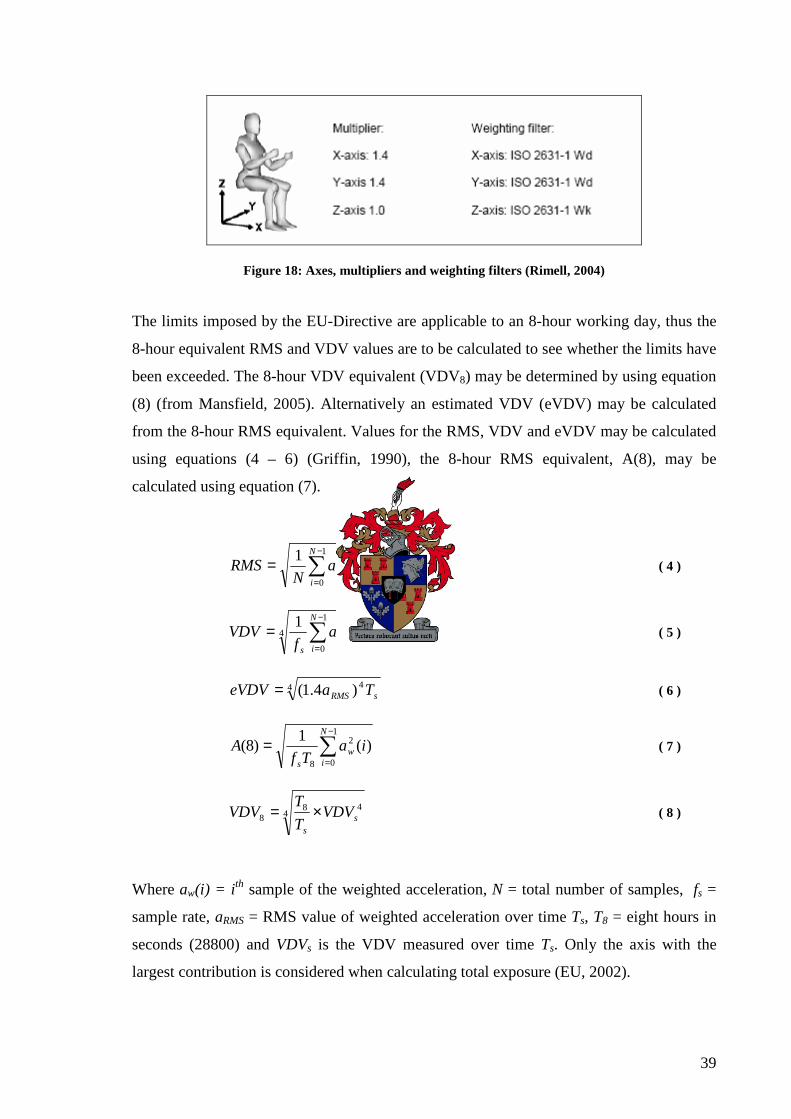
39
Figure 18: Axes, multipliers and weighting filters (Rimell, 2004)
The limits imposed by the EU-Directive are applicable to an 8-hour working day, thus the
8-hour equivalent RMS and VDV values are to be calculated to see whether the limits have
been exceeded. The 8-hour VDV equivalent (VDV8) may be determined by using equation
(8) (from Mansfield, 2005). Alternatively an estimated VDV (eVDV) may be calculated
from the 8-hour RMS equivalent. Values for the RMS, VDV and eVDV may be calculated
using equations (4 – 6) (Griffin, 1990), the 8-hour RMS equivalent, A(8), may be
calculated using equation (7).
∑−
=
=1
0
2 )(1 N
iw ia
NRMS ( 4 )
4
1
0
4 )(1∑
−
==
N
iw
s
iaf
VDV ( 5 )
4 4)4.1( sRMS TaeVDV = ( 6 )
∑−
==
1
0
2
8
)(1
)8(N
iw
s
iaTf
A ( 7 )
448
8 ss
VDVT
TVDV ×= ( 8 )
Where aw(i) = i th sample of the weighted acceleration, N = total number of samples, fs =
sample rate, aRMS = RMS value of weighted acceleration over time Ts, T8 = eight hours in
seconds (28800) and VDVs is the VDV measured over time Ts. Only the axis with the
largest contribution is considered when calculating total exposure (EU, 2002).

40
The Health and Safety Executive (HSE) in the United Kingdom has developed a whole-
body vibration exposure calculator. This calculator allows daily exposures to WBV to be
compared with the EAV and ELV. Once the frequency weighted vibration exposures
multiplied by the correct scaling factors and the exposure times are defined, the calculator
uses equations (7) and (8) to calculate the 8-hour equivalent exposures. The calculator also
calculates the time required to reach the EAV and ELV with the measured RMS and VDV.
The calculator was used for the measurements recorded in Appendix A.
In this chapter the procedure for evaluating whole body vibration exposure was explained.
The raw data is weighed and scaled according to ISO standards and is then converted to an
RMS or VDV value so that the severity of the exposure may be assessed.

41
Chapter 5: Optimisation
During the hauling periods, the truck is driven as fast as possible and the driver cannot do
much to reduce the exposure levels (measured as RMS or VDV). At the loading and
dumping sites, the road is usually very rough, and the truck is driven much slower. The
level of exposure is highly dependent on the driving style (line and speed) of the driver. It
was decided to focus the optimisation study on the hauling periods, as an improvement in
the suspension during the other periods could lead to more aggressive driving (the driver
would not slow down as much when the road gets rough) and similar exposure levels. This
is discussed further in Appendix A. The haul road used for the optimisation resembled a
“very rough dirt road” as described by Cebon (1999), see Chapter 3.3.
From basic calculus we know that for a point in a function to be a minimum, the partial
derivatives (gradient) of the function with respect to its design variables must be zero and
the function needs to be upwards concave at that point. In the general n-dimensional case
this translates into the requirement that the Hessian matrix (the matrix of second partial
derivatives of the function with respect to the design variables) be positive definite. If the
variables are restricted to values within a specific range, the optimal (minimum) point is a
little harder to find. Numerical methods are usually used to find the minimum of such
functions. The non-linear constrained optimisation problem is written mathematically as:
Minimise: F(X) objective function ( 9 )
Subject to:
gj(X) ≤ 0 j = 1, m inequality constraints ( 10 )
hk(X) = 0 k = 1, l equality constraints ( 11 )
Xil ≤ Xi ≤ Xi
u i = 1, n side constraints ( 12 )
where X is the vector of design variables.
To reduce computational time, it is desirable to limit the number of design variables. By
coupling the stiffness and damping of the suspension components (i.e. adjusting them
together such that a 10% increase in the stiffness is accompanied by a 10% increase in

42
damping and vice versa), the number of design variables could be halved. Six design
variables (Xi) were identified for optimisation, they were:
• The struts’ stiffness and damping,
• The cab mounts’ stiffness and damping,
• The tires’ stiffness and damping,
• The sandwich blocks’ stiffness and damping,
• The seat’s stiffness and damping,
• The walking beams’ torsion springs’ stiffness and damping.
Since the influence of the optimised suspension parameters on the handling of the vehicle
was not investigated, it was decided to limit the search for an optimal solution to ±20% of
the current linearized values. The struts and seat, however, were allowed to be even softer
(-40%) as research from literature showed that the rolling stiffness of the steering axle
usually is much higher than required (Fu et al., 2002, and Cebon, 1999) and the seat does
not contribute to the handling of the vehicle. The roll stiffness could also be increased later
by adding a torsion bar to the front suspension. These limits were introduced as side
constraints (equation (12)). No inequality or equality constraints (equations (10) and (11))
were necessary.
5.1 Objective Function
The objective function is the function that is to be minimised by the optimisation
algorithm. The comfort of the truck is represented by the RMS or VDV values. The lower
these values are, the more comfortable the truck will be. The objective of the optimisation
is thus to minimise the RMS or VDV measured at the seat/human interface. For the
purpose of this optimisation study the RMS and VDV values of the weighted vibration data
of all three axes were calculated at the seat/human interface for different suspension setups
as defined by the face centred cube central composite design methodology (see Chapter 2.7
and Figure 2) and were recorded. Separate quadratic response surfaces were fitted to the
recorded results of the RMS and VDV values for each axis.
For three variables (X1, X2, X3), the equation of a quadratic response surface is of the form:
...)( 3322110 ++++= XbXbXbbXF (linear terms)
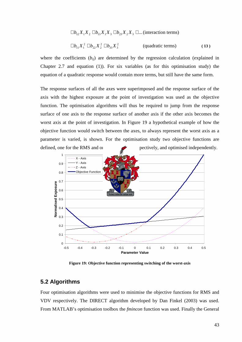
43
...322331132112 ++++ XXbXXbXXb (interaction terms)
2333
2222
2111 XbXbXb +++ (quadratic terms) ( 13 )
where the coefficients (bij) are determined by the regression calculation (explained in
Chapter 2.7 and equation (1)). For six variables (as for this optimisation study) the
equation of a quadratic response would contain more terms, but still have the same form.
The response surfaces of all the axes were superimposed and the response surface of the
axis with the highest exposure at the point of investigation was used as the objective
function. The optimisation algorithms will thus be required to jump from the response
surface of one axis to the response surface of another axis if the other axis becomes the
worst axis at the point of investigation. In Figure 19 a hypothetical example of how the
objective function would switch between the axes, to always represent the worst axis as a
parameter is varied, is shown. For the optimisation study two objective functions are
defined, one for the RMS and one for the VDV respectively, and optimised independently.
0
0.1
0.2
0.3
0.4
0.5
0.6
0.7
0.8
0.9
1
-0.5 -0.4 -0.3 -0.2 -0.1 0 0.1 0.2 0.3 0.4 0.5
Parameter Value
Nor
mal
ised
Exp
osur
e
X - Axis
Y - Axis
Z - Axis
Objective Function
Figure 19: Objective function representing switching of the worst-axis
5.2 Algorithms
Four optimisation algorithms were used to minimise the objective functions for RMS and
VDV respectively. The DIRECT algorithm developed by Dan Finkel (2003) was used.
From MATLAB’s optimisation toolbox the fmincon function was used. Finally the General

44
Reduced Gradient (GRG) and Sequential Quadratic Programming (SQP) algorithms from
ADAMS/INSIGHT were used.
The DIRECT (Divided Rectangles) algorithm is a global optimization scheme which can
be tuned for both local and global properties. It begins at the centre of the design space (the
starting point) and divides the design space into smaller rectangles. The algorithm
iteratively continues this process of electing and subdividing those rectangles that have the
highest likelihood of producing an objective function lower than the current lowest value.
It is this process of subdividing the rectangles that the algorithm achieves both global and
local properties. Unlike the genetic algorithm which is a global scheme, DIRECT is a
deterministic process and needs to be run only once. A disadvantage of this scheme is that
it only terminates after a certain number of iterations have been achieved. For more
information on how this algorithm operates, see E.S. Siah, P. Papalambros and J.L. Volakis
(2002).
Unlike DIRECT, the other three algorithms are gradient based methods. In gradient based
algorithms, information about the first (or second) derivative of the objective function is
used to determine the optimal solution. With such methods it is difficult to know whether
the solution has converged to a global or a local minimum. The DIRECT algorithm
(although slightly more coarse than the other algorithms implemented) could be used to
check whether a global minimum was obtained by the other algorithms.
The GRG method implemented in ADAMS/INSIGHT is an extension of an earlier reduced
gradient method which solved equality-constrained problems only. This is accomplished
by adding slack variables to each inequality constraint (or side constraint in our case) to
make them equality constraints. The method uses first order (gradient) information only to
determine the search direction. The algorithm is well suited to this optimisation problem
since the objective function is not highly non-linear (which could lead the one-dimensional
search to become ill-conditioned) and there were not many inequality constraints (side
constraints only). The number of independent variables would thus not become too large,
requiring lots of memory and making the algorithm inefficient. A detailed description of
this algorithm is given in Vanderplaats (2001) Chapter 6.7 and Rao (1996) Chapter 7.9.

45
The fmincon function in MATLAB’s optimisation toolbox uses a SQP method. Unlike the
GRG method, the SQP method also uses second order (curvature) information to determine
the search direction. The method is also more robust as it ensures that the positive
definiteness of the Hessian is maintained, can cope with inequality and equality constraints
and deals internally with infeasible designs. The SQP method is perhaps one of the best
methods of optimisation as it incorporates the best features of several concepts
(Vanderplaats, 2001). The algorithm is well suited to this optimisation problem as the
objective function is quadratic and the constraints linear. The SQP method implemented in
fmincon differs slightly from the SQP method used in ADAMS/INSIGHT. Although the
general strategy is the same, the sub-problems are solved differently. The fmincon function
in MATLAB could thus be used to verify the solutions of the ADAMS/INSIGHT
algorithms (and vice versa). For more information on how this function operates, see
MATLAB Optimisation toolbox User’s Guide (2004). A detailed description of how the
SQP method from ADAMS/INSIGHT operates is given in Vanderplaats (2001) Chapter
6.9 and Rao (1996) Chapter 7.10.
In this chapter the design variables, constraints, objective functions and algorithms that are
used in the optimisation study is discussed. The optimisation will focus on reducing the
vibration exposure in the worst-axis (as defined by the objective function and Figure 19)
only.

46
Chapter 6: Results
The optimisation procedure followed is summarised in three consecutive tasks. The first
task (discussed in the first section of this chapter) was to investigate the influence of the
design variables on the results. This was done by varying the design variables (suspension
parameters) over the allowed range and determining the influence they have on the
response. The second task (discussed in the second section of this chapter) was to apply the
optimisation algorithms discussed in the previous chapter to the objective functions
(response surfaces) to obtain the suspension parameters that will provide the lowest
vibration exposure on the driver. The third task (discussed in the third section of this
chapter) was to verify the optimal solution by exposing the truck to different road inputs
under different loading conditions using the optimised suspension characteristics.
The results from each task are divided into three subsections. The first subsection focuses
on the truck whilst unloaded. The second subsection focuses on the truck whilst loaded.
The third subsection focuses on a combined cycle, i.e. first unloaded, then loaded
travelling the same section of road; as normally occurs in practice. The parameters were
optimised within the prescribed limits for RMS and VDV values, evaluated according to
ISO 2631 (1997), for each of the subsections discussed above.
6.1 Influence of Design Variables
To determine the influence of a design variable on the response, all the variables are kept
constant while the variable being investigated is varied over its entire allowed range. The
Effect % is defined as the ratio of the change in response to the neutral (unchanged truck)
response expressed as a percentage (see equation (14)). It will be negative for a variable
that causes a decrease in the response with an increase in stiffness.
%100)(
)()(%_ ×−=
neutralExposure
softExposurestiffExposureEffect ( 14 )
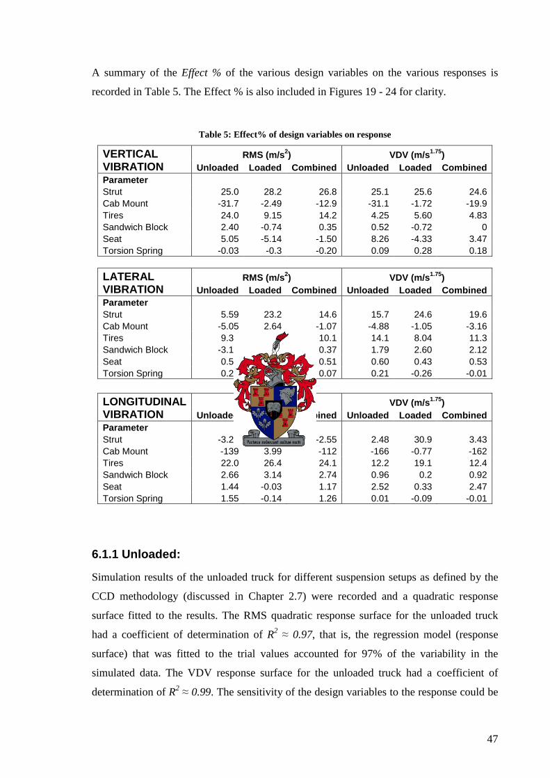
47
A summary of the Effect % of the various design variables on the various responses is
recorded in Table 5. The Effect % is also included in Figures 19 - 24 for clarity.
Table 5: Effect% of design variables on response
VERTICAL RMS (m/s 2) VDV (m/s 1.75) VIBRATION Unloaded Loaded Combined Unloaded Loaded Combined Parameter Strut 25.0 28.2 26.8 25.1 25.6 24.6 Cab Mount -31.7 -2.49 -12.9 -31.1 -1.72 -19.9 Tires 24.0 9.15 14.2 4.25 5.60 4.83 Sandwich Block 2.40 -0.74 0.35 0.52 -0.72 0 Seat 5.05 -5.14 -1.50 8.26 -4.33 3.47 Torsion Spring -0.03 -0.3 -0.20 0.09 0.28 0.18
LATERAL RMS (m/s 2) VDV (m/s 1.75) VIBRATION Unloaded Loaded Combined Unloaded Loaded Combined Parameter Strut 5.59 23.2 14.6 15.7 24.6 19.6 Cab Mount -5.05 2.64 -1.07 -4.88 -1.05 -3.16 Tires 9.30 10.7 10.1 14.1 8.04 11.3 Sandwich Block -3.16 3.77 0.37 1.79 2.60 2.12 Seat 0.56 0.41 0.51 0.60 0.43 0.53 Torsion Spring 0.22 -0.07 0.07 0.21 -0.26 -0.01
LONGITUDINAL RMS (m/s 2) VDV (m/s 1.75) VIBRATION Unloaded Loaded Combined Unloaded Loaded Combined Parameter Strut -3.25 2.21 -2.55 2.48 30.9 3.43 Cab Mount -139 3.99 -112 -166 -0.77 -162 Tires 22.0 26.4 24.1 12.2 19.1 12.4 Sandwich Block 2.66 3.14 2.74 0.96 0.2 0.92 Seat 1.44 -0.03 1.17 2.52 0.33 2.47 Torsion Spring 1.55 -0.14 1.26 0.01 -0.09 -0.01
6.1.1 Unloaded:
Simulation results of the unloaded truck for different suspension setups as defined by the
CCD methodology (discussed in Chapter 2.7) were recorded and a quadratic response
surface fitted to the results. The RMS quadratic response surface for the unloaded truck
had a coefficient of determination of R2 ≈ 0.97, that is, the regression model (response
surface) that was fitted to the trial values accounted for 97% of the variability in the
simulated data. The VDV response surface for the unloaded truck had a coefficient of
determination of R2 ≈ 0.99. The sensitivity of the design variables to the response could be

48
determined from the response surfaces. The response surface also described the variability
well enough to be used as the objective function in the optimisation of the RMS and VDV
exposure levels (see equation (1)) as the R2 values for both exceeded 0.9.
In Figure 20 and Figure 21 the influence of the variables on the RMS and VDV in the
direction of the main axes is recorded. The light-coloured bars represent a negative Effect
%, indicating that increasing the stiffness will reduce the exposure level. From Table 5,
Figure 20 and Figure 21 it may be seen that for the unloaded truck the cab mounts, struts
and tires have the largest influence on the responses. It is seen that improving one response
may lead to a deterioration of another (reducing the stiffness of the sandwich blocks leads
to a reduction in vertical and longitudinal RMS, but an increase in the lateral RMS) and
that each response is not equally influenced (cab mounts influence the vibrations in the
longitudinal direction by up to 139%, the vertical by 31% and the lateral by 5% when
varied over the same range).
Factor Effect % Cab Mount -31.7
Strut 25
Tires 24
Seat 5.05
Sandwich Block 2.4
Torsion Spring -0.03
Factor Effect % Tires 9.3
Strut 5.59
Cab Mount -5.05
Sandwich Block -3.16
Seat 0.56
Torsion Spring 0.22
Factor Effect % Cab Mount -139
Tires 22
Strut -3.25
Sandwich Block 2.66
Torsion Spring 1.55
Seat 1.44
RMS Longitudinal Vibration
RMS Lateral Vibration
RMS Vertical Vibration
Figure 20: Influence of variables of unloaded truck on RMS

49
Factor Effect % Cab Mount -31.1
Strut 25.1
Seat 8.26
Tires 4.25
Sandwich Block 0.52
Torsion Spring 0.09
Factor Effect % Strut 15.7
Tires 14.1
Cab Mount -4.88
Sandwich Block 1.79
Seat 0.6
Torsion Spring 0.21
Factor Effect % Cab Mount -166
Tires 12.2
Seat 2.52
Strut 2.48
Sandwich Block 0.96
Torsion Spring 0.01
VDV Lateral Vibration
VDV Longitudinal Vibration
VDV Vertical Vibration
Figure 21: Influence of variables of unloaded truck on VDV
6.1.2 Loaded:
Simulation results of the loaded truck for different suspension setups as defined by the
CCD methodology were recorded and a quadratic response surface fitted to the results. The
RMS quadratic response surface for the loaded truck had a coefficient of determination of
R2 ≈ 0.93, that is, the regression model (response surface) accounts for 96% of the
variability in the simulated data. The VDV response surface for the loaded truck had a
coefficient of determination of R2 ≈ 0.99. The sensitivity of the design variables to the
response could be determined from the response surfaces. The response surfaces could also
be used as the objective function in the optimisation of the RMS and VDV exposure levels
(see equation (1)) as the R2 values for both exceeded 0.9.
In Figure 22 and Figure 23 the influence of the variables on the RMS and VDV in the
direction of the main axes is recorded. The light-coloured bars represent a negative Effect

50
%, indicating that increasing the stiffness will reduce the exposure level. From Table 5,
Figure 22 and Figure 23 it may be seen that for the loaded truck the struts and tires have
the largest influence on the responses. The cab mounts do not influence the responses as
much as for the unloaded truck. It is again seen that improving one response may lead to a
deterioration of another (reducing the stiffness of the sandwich blocks, cab mounts and seat
leads to a reduction in vertical RMS, but an increase in the lateral and longitudinal RMS)
and that each response is not equally influenced (struts influence the vibrations in the
vertical and longitudinal directions by approximately 25%, but the longitudinal direction
by only 2% when varied over the same range.)
Studying Table 5, or Figures 19 to 22, it is interesting to note that all the variables (except
the tires) have had a change in sign for the Effect % in at least one of their responses. This
will cause the optimal solution to change as the loading condition is changed from
unloaded to loaded.
Factor Effect % Strut 28.2
Tires 9.15
Seat -5.14
Cab Mount -2.49
Sandwich Block -0.74
Torsion Spring -0.3
Factor Effect % Strut 23.2
Tires 10.7
Sandwich Block 3.77
Cab Mount 2.64
Seat 0.41
Torsion Spring -0.07
Factor Effect % Tires 26.4
Cab Mount 3.99
Sandwich Block 3.14
Strut 2.21
Torsion Spring -0.14
Seat -0.03
RMS Vertical Vibration
RMS Lateral Vibration
RMS Longitudinal Vibration
Figure 22: Influence of variables of loaded truck on RMS

51
Factor Effect % Strut 25.6
Tires 5.6
Seat -4.33
Cab Mount -1.72
Sandwich Block -0.72
Torsion Spring 0.28
Factor Effect % Strut 24.6
Tires 8.04
Sandwich Block 2.6
Cab Mount -1.05
Seat 0.43
Torsion Spring -0.26
Factor Effect % Strut 30.9
Tires 19.1
Cab Mount -0.77
Seat 0.33
Sandwich Block 0.2
Torsion Spring -0.09
VDV Lateral Vibration
VDV Longitudinal Vibration
VDV Vertical Vibration
Figure 23: Influence of variables of loaded truck on VDV
6.1.3 Combined:
The simulation results obtained for different suspension setups as defined by the CCD
methodology of the loaded and unloaded truck were combined, recorded and a quadratic
response surface fitted to the results. The RMS response surface of the combined cycle had
a coefficient of determination of R2 ≈ 0.96, that is, the regression model (response surface)
accounts for 96% of the variability in the simulated data. The VDV response surface for
the combined cycle had R2 ≈ 0.99. The sensitivity of the design variables to the response
could be determined from the response surface. It also meant that the response surface
described the variability well enough to be used as the objective function in the
optimisation of the RMS and VDV exposure levels (see equation (1)) as the R2 value for
both exceeded 0.9.

52
In Figure 24 and Figure 25 the influence of the variables on the RMS and VDV in the
direction of the main axes is recorded. The light-coloured bars represent a negative Effect
%, indicating that increasing the stiffness will reduce the exposure level. From Table 5,
Figure 24 and Figure 25 it may be seen that for the combined cycle the struts, cab mounts
and tires have the largest influence on the responses. The combined cycle’s responses are a
weighted combination of the results obtained from the loaded and unloaded truck.
Optimising the combined results should give improvements for the loaded and unloaded
truck, but will not necessarily be the optimal solution for either response.
Factor Effect % Strut 26.8
Tires 14.2
Cab Mount -12.9
Seat -1.5
Sandwich Block 0.35
Torsion Spring -0.2
Factor Effect % Strut 14.6
Tires 10.1
Cab Mount -1.17
Seat 0.51
Sandwich Block 0.37
Torsion Spring 0.07
Factor Effect % Cab Mount -112
Tires 24.1
Sandwich Block 2.74
Strut -2.55
Torsion Spring 1.26
Seat 1.17
RMS Vertical Vibration
RMS Lateral Vibration
RMS Longitudinal Vibration
Figure 24: Influence of variables of combined cycle on RMS

53
Factor Effect % Strut 24.6
Cab Mount -19.9
Tires 4.83
Seat 3.47
Torsion Spring 0.18
Sandwich Block 0
Factor Effect % Strut 19.9
Tires 11.3
Cab Mount -3.16
Sandwich Block 2.12
Seat 0.53
Torsion Spring -0.01
Factor Effect % Cab Mount -162
Tires 12.4
Strut 3.43
Seat 2.47
Sandwich Block 0.92
Torsion Spring -0.01
VDV Lateral Vibration
VDV Longitudinal Vibration
VDV Vertical Vibration
Figure 25: Influence of variables of combined cycle on VDV
6.2 Optimal Parameters
It is important to note that the EU-Directive currently requires the axis with highest
vibration to not exceed the exposure levels. The suspension is thus optimised for the worst
axis only, which may cause the response of another axis to improve or deteriorate. Should
the response of another axis deteriorate to such an extent that it becomes the worst axis; the
objective function is adapted to continue optimising that axis’ response (see Figure 19).
6.2.1 Unloaded:
The objective function for the unloaded truck was optimised by using the different
optimisation algorithms explained previously. The solutions (recorded in Table 6 and
Table 7) indicate the relative stiffness of the optimal parameter to the current linearized
parameter. A value of, for example, 1.2 indicates that the optimal parameter is 20% stiffer

54
than the current linearized parameter, while a value of 0.8 indicates that the optimal
parameter is 20% less stiff than the current linearized parameter.
The worst axis for this test condition was the lateral axis. Improvements for all the axes
were, however, achieved. The optimal solutions for the RMS and VDV exposures were
confirmed by more than one algorithm. Only the greatest improvement is converted into a
percentage. The grey blocks show for which algorithm the greatest improvement was
achieved. It was discovered that an 18.5% reduction in RMS and 31% reduction in VDV is
attainable within the given constraints (albeit not at the exact same suspension setting).
Table 6: Unloaded optimal suspension parameters for RMS exposure
MATLAB ADAMS Optimisation Algorithm Nominal DIRECT fmincon SQP GRG
Strut 1 0.61 0.6 0.6 0.6
Cab Mount 1 1.18 1.2 1.2 1.2 Tires 1 0.8 0.8 0.8 0.8
Sandwich Block 1 0.99 1 1 1
Seat 1 0.9 0.6 0.6 0.6 Torsion Spring 1 1 1.1 1.1 1.1
RMS (m/s 2) % Improvement Vertical 0.114 0.062 0.060 0.060 0.060 47.2 Lateral 0.226 0.190 0.184 0.184 0.184 18.5
Longitudinal 0.140 0.080 0.083 0.083 0.083 42.9
Table 7: Unloaded optimal suspension parameters for VDV exposure
MATLAB ADAMS Optimisation Algorithm Nominal DIRECT fmincon SQP GRG
Strut 1 0.61 0.6 0.6 0.6
Cab Mount 1 1.1 1.1 1.1 1.1 Tires 1 0.8 0.8 0.8 0.8
Sandwich Block 1 0.8 0.8 1 1
Seat 1 0.9 0.8 0.6 0.6 Torsion Spring 1 1 1.1 1.1 1.1
VDV (m/s 1.75) % Improvement Vertical 0.373 0.232 0.229 0.220 0.220 40.8 Lateral 0.685 0.477 0.474 0.473 0.473 31.0
Longitudinal 0.496 0.240 0.245 0.245 0.245 51.7

55
6.2.2 Loaded:
The objective function for the loaded truck was optimised by using the different
optimisation algorithms explained previously. The solutions (recorded in Table 8 and
Table 9) indicate the relative stiffness of the optimal parameter to the current linearized
parameter. It is again seen that while optimising the worst axis (the lateral axis for this load
condition), improvements for all the axes were achieved. All the algorithms produced
similar improvements. Only the greatest improvement is converted into a percentage. The
grey blocks show for which algorithm the greatest improvement was achieved. It was
discovered that a 38.6% reduction in the RMS and 33.8% reduction in VDV is attainable
within the given constraints (albeit not at the exact same suspension settings, as VDV is
lower when cab mounts are hard and seat soft, while RMS is just the opposite).
Table 8: Loaded optimal suspension parameters for RMS exposure
MATLAB ADAMS Optimisation Algorithm Nominal DIRECT fmincon SQP GRG
Strut 1 0.62 0.61 0.61 0.61
Cab Mount 1 0.82 0.8 0.8 0.8 Tires 1 0.8 0.8 0.8 0.8
Sandwich Block 1 0.8 0.8 0.8 0.8
Seat 1 0.9 0.98 1 1 Torsion Spring 1 1 1.1 1.1 1.1
RMS (m/s 2) % Improvement Vertical 0.147 0.101 0.100 0.100 0.099 32.4 Lateral 0.312 0.194 0.191 0.191 0.191 38.6
Longitudinal 0.079 0.052 0.052 0.051 0.051 34.9
Table 9: Loaded optimal suspension parameters for VDV exposure
MATLAB ADAMS Optimisation Algorithm Nominal DIRECT fmincon SQP GRG
Strut 1 0.68 0.67 0.67 0.67
Cab Mount 1 1.19 1.2 1.2 1.2 Tires 1 0.83 0.85 0.85 0.85
Sandwich Block 1 0.8 0.8 0.8 0.8
Seat 1 0.9 0.6 0.6 0.6 Torsion Spring 1 1 1.1 1.1 1.1
VDV (m/s 1.75) % Improvement Vertical 0.337 0.255 0.262 0.262 0.262 24.5 Lateral 0.736 0.490 0.487 0.487 0.487 33.8
Longitudinal 0.209 0.137 0.139 0.139 0.139 34.4

56
6.2.3 Combined:
The objective function for the combined loaded/unloaded cycle was optimised by using the
different optimisation algorithms explained previously. The solutions (recorded in Table
10 and Table 11) indicate the relative stiffness of the optimal parameter to the current
linearized parameter. Improvements for all the axes were achieved although the algorithms
were only optimising the worst axis (mostly the lateral axis). All the algorithms produced
similar improvements. Only the greatest improvement is converted into a percentage. The
grey blocks show for which algorithm the greatest improvement was achieved. It was
discovered that a 29.8% reduction in the RMS and 27.4% reduction in VDV is attainable
within the given constraints for the worst axis (albeit not at the exact same suspension
settings).
Table 10: Combined optimal suspension parameters for RMS exposure
MATLAB ADAMS Optimisation Algorithm Nominal DIRECT fmincon SQP GRG
Strut 1 0.6 0.6 0.6 0.6
Cab Mount 1 1.18 1.2 1.2 1.2 Tires 1 0.8 0.8 0.8 0.8
Sandwich Block 1 0.99 0.8 1 1
Seat 1 0.9 0.85 1.04 1.05 Torsion Spring 1 1 1.1 1.1 1.1
RMS (m/s 2) % Improvement Vertical 0.137 0.082 0.079 0.080 0.080 42.3 Lateral 0.279 0.198 0.197 0.196 0.196 29.8
Longitudinal 0.117 0.069 0.077 0.069 0.069 41.3
Table 11: Combined optimal suspension parameters for VDV exposure
MATLAB ADAMS Optimisation Algorithm Nominal DIRECT fmincon SQP GRG
Strut 1 0.62 0.62 0.61 0.6
Cab Mount 1 1.13 1.13 1.1 1.12 Tires 1 0.81 0.82 0.8 0.81
Sandwich Block 1 0.8 0.8 1 0.87
Seat 1 0.9 0.6 0.6 0.6 Torsion Spring 1 1 1.1 1.1 1.1
VDV (m/s 1.75) % Improvement Vertical 0.422 0.279 0.279 0.273 0.277 35.3 Lateral 0.800 0.584 0.582 0.581 0.583 27.4
Longitudinal 0.446 0.242 0.241 0.246 0.243 46.1

57
Each loading condition and each road input would have a different optimal solution as is
seen from the optimal parameters obtained in the previous section. It does, however,
appear as though the following adjustments (from Table 10) would give the largest
improvement in RMS and VDV for all conditions:
• Front struts (spring and damper) should be softened by 40%
• Cab mounts should be stiffened by 20%
• Tires should be softened by 20%
• Sandwich blocks should remain as simulated
• Seat should remain as simulated
• Torsion springs should be stiffened by 10%
The adjustments to the front struts, cab mounts and tires are limited by the side constraints
discussed in Chapter 5. This corresponds well with results published by Jiang (2001) who
reported in his literature study that when optimizations were unconstrained, negative
damping appears, showing that energy (active suspensions) are required for an optimal
solution.
6.3 Verification
To verify the “optimal solution” the VDV and RMS exposures of the “optimal” truck were
compared to the exposures of the original truck under different loading conditions and road
surface inputs as described by Cebon (1999), ISO 8608 (1995) and Wong (1978). The
trucks were simulated as travelling at a speed of 10m/s. The simulation results are recorded
in Table 12 as a percentage improvement in exposure level. The “optimal” road represents
the road surface that was used for the optimisation study. Positive entries indicate a
reduction in exposure while negative entries indicate an increase in exposure level for the
“optimal” setting. The bold entries indicate the worst-axis for the respective load condition
and road surface of the original truck. The grey blocks indicate the worst-axis for the
respective load condition and road surface of the optimised truck. The “worst axis”
columns indicate the direct percentage improvement between initial and final worst axes.
From Table 12 it is seen that the optimised suspension does lead to higher vibration
exposures in certain cases (indicated by negative entries). It was, however, found that all

58
the axes (and in particular the worst axes) were improved for all the road types when the
vibration exposure levels of the loaded and unloaded conditions were considered together
(combined model). For example; the optimised suspension increased lateral vibrations on
the seat (Seat Top X) by 85.3% (RMS) when the truck was driven over a very poor road
surface in the loaded condition, but reduced Seat Top X vibration exposure level by 90.7%
(RMS) in the unloaded condition for the same road surface. The overall combined effect of
the optimised suspension for the loaded and unloaded truck driving over the very poor road
surface was to reduce the Seat Top X vibration exposure by 83.9% (RMS).
Generally, as the road surface deteriorates, the percentage improvements achieved by the
“optimal” suspension also diminish (although the absolute improvement may increase or
stay the same). It may also be noticed that the worst axis changes depending on load
condition, road input and method of evaluation. The worst axis may also be different after
the optimal parameters are applied to the original truck. The combined cycle of the original
truck on a good road, for example, had the lateral direction as the worst axis. A larger
improvement in the lateral direction than the vertical direction during the optimisation has
lead to the vertical direction becoming the new worst axis for VDV measurements and the
longitudinal direction becoming the new worst axis for RMS measurements.
Table 12: % Improvement with optimal parameters on different road surfaces
RMS VDV Model Road Seat
Top Z Seat
Top Y Seat
Top X Worst axis
Seat Top Z
Seat Top Y
Seat Top X
Worst axis
Good 39.0 -110.9 86.2 79.5 46.1 70.9 76.8 66.7
Poor 56.6 64.5 92.0 88.2 49.5 67.4 79.9 71.1
Very Poor 56.1 79.9 90.7 86.3 35.3 79.4 70.8 58.1
Optimal 45.9 16.4 49.0 16.4 35.4 31.0 50.6 31.0
Unloaded
Plowed Field 35.1 25.7 83.6 75.8 7.6 32.7 41.2 16.0
Good 93.6 99.9 62.9 97.6 78.5 99.7 73.3 94.4
Poor 91.9 80.4 86.2 89.6 89.5 89.9 79.1 89.5
Very Poor -35.4 16.5 -85.3 -82.4 -19.1 36.0 -26.9 -19.1
Optimal 31.8 33.9 31.9 33.9 31.1 29.3 40.5 29.3
Loaded
Plowed Field -26.3 57.7 -68.8 -62.2 -14.3 46.3 -20.3 -14.3
Good 89.1 99.7 77.7 97.2 68.0 99.4 76.2 91.4
Poor 86.9 68.3 89.3 88.6 83.6 67.8 79.8 83.6
Very Poor 47.5 72.9 83.9 83.2 34.7 79.3 70.5 57.8
Optimal 36.7 26.9 44.7 26.9 33.6 30.0 50.2 30.0
Combined
Plowed Field 31.0 41.0 78.9 73.7 7.5 32.8 41.2 16.0
Bold numbers indicate original suspension’s worst-axis; Grey blocks indicate optimised suspension’s worst-axis

59
To verify whether a softer seat suspension would not give better solutions, the experiments
were repeated with the seat softened by 40% (as suggested by Table 11). It was discovered
that for good road surfaces, i.e. where the end-stops are not engaged, the softer seat gave
even lower exposure levels (in RMS and VDV), but when the road surface became
rougher, the advantage shrank and, for the worst road surface (ploughed field), the
exposure levels in all axis were reduced by a smaller amount than they could have been
had the seat stiffness not been changed. The difference of improvement in worst axis
exposure level between a softened seat and the current seat, with the other suspension
systems set to optimal, was usually less than 2% for all loading conditions and road
surfaces. It was thus decided to keep the seat as it is.

60
Chapter 7: Conclusions and Recommendations
The introduction of the EU-Directive that limits vibration exposure means that suspension
systems on ADTs need to be optimised for improved vibration comfort. In order to
optimise the suspension systems for comfort a reliable model of the truck is needed. A
literature study of modelling techniques was completed to determine which assumptions
may be made to simplify the model of such a truck. It was established that a variety of
models have been tried over the years and that some simplified models did in fact give
reliable results.
The three major components of a simulation model is the road input, the truck and the
human driver. The road may be reconstructed from PSD measurements of similar road
surfaces and introduced to the model through vertical actuators. The truck was simplified
by ignoring the steering and drive-train and constraining some degrees of freedom. The
human and seat was modelled with a lumped parameter model obtained from literature.
The suspension parameters were linearized over the entire range of motion and the
linearization was validated by three MATLAB models of increasing complexity and
degrees of freedom. The results from the MATLAB models were compared to those of a
truck driving over irregular terrain and it was shown that after the linearization of the
parameters the model still generates realistic results.
To model the truck even more accurately a 24 degrees of freedom model was developed in
ADAMS/VIEW. The ADAMS/VIEW model was verified by comparing the results to a
previously (and independently) developed 50 degree-of-freedom ADAMS/CAR model as
well as measured results from a truck traversing a sinusoidal obstacle. The ADAMS/VIEW
model correlated very well with the measured results when large displacements were
present. The model’s accuracy was slightly lower when the displacements were small. This
is mainly due to the linearization which is better suited for large displacements.
The influence of each suspension system parameter was investigated to determine the
relative importance of each parameter on the vibration exposure. The parameters that
needed to be optimised were identified together with four different optimisation

61
algorithms. A surface response function of each exposure was constructed and used as the
objective function in each of the optimisation algorithms.
An optimisation study was performed and the optimal suspension parameters identified.
The parameters were then verified by comparing exposure levels from the original truck
with the optimised truck as it traverses different road surfaces. It was discovered that the
optimised parameters gave improvements for all road surfaces for the combined
(loaded/unloaded) cycle.
The main conclusions that may be derived from this research are:
• A simplified, reduced order simulation model of an ADT can be used for
optimisation studies to reduce vibration exposure levels of the driver.
One of the objectives of the project was to determine whether a simplified reduced order
model could be used to optimise the suspension parameters. By making the correct
assumptions the complexity of a model can be reduced significantly while still producing
reliable results. The 24-DOF model that was developed in ADAMS/VIEW accurately
simulates the vibration exposure levels on the driver. The model can be used to investigate
the influence of the suspension parameters on the exposure levels and can be simulated
with different load conditions and road surface inputs. It was shown that the model is more
accurate at predicting the vibration exposure than the 50-DOF model developed in
ADAMS/CAR for a particular input. The model is, however, not suited for handling
studies as it does not include a drive train or steering mechanism, neither is it suitable for
component fatigue studies.
• The horizontal directions may have higher vibration levels than the vertical
direction for specific load conditions and road inputs.
Most suspension components are designed to only isolate the driver from vertical
vibration. From Table 12 it is seen that more than 80% of the conditions originally
investigated had one of the horizontal axes as the worst axis. Measurements taken on a
truck at a construction site (reported in Appendix A) also indicated that the horizontal axis
often contribute larger exposure levels than the vertical direction even after applying the
appropriate weighting factors.

62
• It is possible to reduce the vibration exposure levels of the driver by changing
the parameters of the passive suspension systems.
Donati (2001) concluded in his article that there are three main ways of reducing vibration
exposure, namely to reduce the source (road improvement, driving style, etc.), to reduce
the transmission by incorporating better suspension systems and by improving the
ergonomics of the cab. It was shown in the previous chapter that the exposure levels of the
driver may be reduced by as much as 99.9% (Loaded truck on good road in Table 12) by
only changing the passive suspension systems’ parameters. It was also shown that finding
the optimal solution for the combined cycle gave improvements for the loaded and
unloaded truck, but was not necessarily the optimal solution for either response. The
improvements in vibration exposure levels were achieved without changing the operation,
layout or physical dimensions of the current suspension systems.
• The largest improvement was obtained by adjusting the stiffness of the front
struts, tires and cab mounts.
Of all the suspension system components, the front struts, tires and cab mounts proved to
have the largest influence on the exposure levels of the driver. Investigating Table 5 and
Figures 19 to 24 it is seen that the cab mounts have the largest influence on the
longitudinal direction (causing the VDV exposure of the unloaded truck to change by as
much as 165.5% if the parameter is varied from 20% stiffer to 20% softer), but also had
significant influence on the vibration exposures in the other directions. The front struts had
the largest influence on the vertical and longitudinal directions (changes of up to 31%
being recorded for the VDV exposure of the longitudinal direction in the loaded truck as
the parameter is varied). The tires make significant contributions to reducing the exposure
levels in all the directions (26.4% change in longitudinal RMS of loaded truck recorded as
parameter is varied) and is the only parameter that always caused a reduction in exposure
(for all directions, loading conditions and evaluation measures) with a reduction in
stiffness. About 95% of the improvements obtained by the optimisation study are as a
result of these three parameters.
• The sandwich blocks, walking beam torsion spring and seat had a small
influence on the vibration exposure of the driver.

63
On their own the sandwich blocks, walking beam torsion springs and seat influenced the
exposure levels of the driver by very small amounts (usually by less than a percent) as they
were varied within the constraint boundaries of the optimisation study. The seat gave a
maximum improvement of 8% in the vertical direction of the unloaded truck, but only
decreased the exposure by 2.5% for the combined cycle. Only about 5% of the
improvements obtained by the optimisation study are attributed to these parameters.
Recommendations for future work:
• The influence of the optimised parameters on the vehicle dynamics should be
investigated.
The model that was used for the optimisation study was not suited for handling studies and
thus the influence of the parameters on the handling of the vehicle was not properly
investigated. The softening of the front struts, tires and cab mounts will compromise the
handling of the vehicle. A study of the influence of the optimal parameters on the
dynamics of the vehicle is required to determine whether the roll stiffness of the steering
axle (which according to Fu et al. (2002) and Cebon (1999) is usually much higher than
required) is still within acceptable limits. The influence of softer tires on tire wear should
also be investigated.
• Suspension systems with isolating capacity in directions other than the vertical
direction should be investigated.
Sankar and Afonso (1993) (quoted in Prasad, 1995) studied the concept of a lateral seat
suspension as a means of improving the ride comfort in off-road vehicles. A computer
parametric study showed that a lateral seat suspension with a dynamic vibration absorber
could improve the ride comfort by 75% while reducing relative displacements by as much
as 7%. Reducing the vibration exposure of lateral and longitudinal vibrations is as
important as reducing the vibration exposure in the vertical direction and should therefore
be investigated.
• The viability of semi-active or active suspensions should be investigated.
Passive suspensions are limited in that they can only truly be optimised for one specific
load condition and road input. Due to the fact that the suspension characteristics in semi-

64
active or active suspensions can be changed according to the terrain requirements, these
types of suspension systems can improve ride quality over a wide spectrum of terrain.
Jiang (2001) reported in his literature study that when optimizations were unconstrained,
negative damping appears, showing that energy (active suspensions) are required for an
optimal solution.
• A study of the viability of other types of suspensions for ADTs (such as air
suspensions) should be commissioned.
It was shown in the literature study that the current suspension setup produces the highest
dynamic forces of all the suspension types commonly used in heavy vehicles. The high
dynamic forces not only lead to higher exposure levels, but also cause the roads to be
damaged faster and may even increase the rate of tire wear. Air suspensions are reported to
produce the smallest dynamic forces (Cebon and Cole, 1992). Through his research
Hostens (2004) has showed that air-spring seat suspensions are better than mechanical-
spring seats. The main reasons for this is that air dampers provide high damping at low
frequencies (by throttling in the orifice), but low damping at high frequencies (due to
choking in the orifice).
The exposure levels that the driver is exposed to are strongly dependent on the driving
style (speed and line). An improvement in the suspension may only lead to more
aggressive driving (not reducing speed when road becomes rough) and thus similar
exposure levels. Maintaining the road surfaces (by regular scraping, for example), to
reduce the inputs from the road, is a vital part in reducing the exposure levels of the driver.
It is the hope of the author that the research presented in this document may prove to be
useful to the manufacturers and industry at large to reduce the vibration exposure levels of
the drivers of ADTs.

65
References
ADAMS/Insight Version 2005, Help Files, MSC.Software Corporation, Santa Ana, CA, USA. Ahmed, O.B. and Goupillon J.F., 1997, Predicting the ride vibration of an agricultural tractor, Journal of Terramechanics, Vol. 34, No 1, pp 1-11.
Brereton, P. and Nelson C., 2004, Progress with implementing the EU Physical Agents (Vibration) Directive in the United Kingdom, 39th United Kingdom Group Meeting on Human Response to Vibration, 15-17 September 2004, pp 293-300, Ludlow, England. Cebon, D., 1999, Handbook of Vehicle-Road Interaction, Advances in Engineering 2, Swets & Zeitlinger, Lisse, the Netherlands. Close, M.C., Frederick D.K., Newell J.C., 2002, Modeling and Analysis of Dynamic Systems, Third Edition, John Wiley \& Sons Inc, New York. Cole, D.J. and Cebon, D., 1994, Predicting Vertical Dynamic Tire Forces of Heavy Trucks, Vehicle-Road Interaction, ASTM, STP 1225, B. T. Kulakowski, Ed., American Society for Testing and Materials, Philadelphia, pp 27-35. Cole, D.J. and Cebon, D., 1992, Validation of an articulated vehicle simulation, Vehicle System Dynamics, Vol. 21, No 4, pp 197–223. Darlington, P. and Tyler, R.G., 2004, Measurement uncertainty in human exposure to vibration, 39th United Kingdom Group Meeting on Human Responses to Vibration, 15-17 September 2004, pp 301-308, Ludlow, England. Deprez, K., Hostens, I., Ramon, H., 2004, Modelling and design of a pneumatic suspension for seats and cabins of mobile agricultural machines, Proceedings of ISMA, 22 September 2004, pp 1185 – 1194. El Madany, M.M., 1988, Active damping and load leveling for ride improvement, Computers & Structures Vol. 29, No. 1, pp. 89-97. El Madany, M.M., 1987, An analytical investigation of isolation systems for cab ride, Computers & Structures Vol. 27, No. 5, pp. 679-688. Esat, I., 1996, Optimisation of a double wishbone suspension system, Engineering Systems Design and Analysis, PD-Vol 81, Vol. 9, ASME, pp. 93-98. EU-Directive, 2002, Directive 2002/44/EC of the European Parliament and of the council of 25 June 2002, Official Journal of the European Communities. Fairley, T.E. and Griffin M.J., 1988, Prediction of the discomfort caused by simultaneous vertical and fore-and-aft whole-body vibration, Journal of Sound and Vibration, Vol. 124, No 1, pp 141-156.

66
Finkel, D.E., 2003, DIRECT Optimization Algorithm User Guide. Technical Report, CRSC, N.C. State University. Donati, P., 2001, Survey of technical preventative measures to reduce whole-body vibration effects when designing mobile machinery, Journal of Sound and Vibration, (2002) Vol. 253, No 1, pp 169-183. Fothergill, L.C. and Griffin, M.J., 1977, The use of an intensity matching technique to evaluate human response to whole-body vibration, Ergonomics, Vol. 20, No 3, pp 249-261, 263-276, 521-533. Fu, T.T. and Cebon, D., 2002, Analysis of a truck suspension database, International Journal of Heavy Vehicle Systems, Vol. 9, No. 4, pp 281-297. Gallais, C., 2004, Duration of whole-body vibration exposure: Evaluating and comparing the changes in comfort between two lateral oscillations at 1Hz and 4Hz, 39th United Kingdom Group Meeting on Human Responses to Vibration, 15-17 September 2004, pp 381-394, Ludlow, England. Gill, P.E., Murray, W. and Wright, M.H., 1981, Practical Optimization, Academic Press, London. Gillespie, T.D., 1992, Fundamentals of Vehicle Dynamics, Society of Automotive Engineers, Warrendale. Gillespie, T.D. and Karamihas, S.M., 2000, Simplified models for truck dynamic response to road inputs, Heavy Vehicle Systems, International Journal of Vehicle Design, Vol. 7, No 1, pp 231-247. Gipser, M., 1999, FTire, a new fast tire model for ride comfort simulations, International ADAMS’ Users Conference, Berlin, Germany. Gouw, G.J., Rakheja, S., Sankar, S., Afework, Y., 1990, Increased comfort and safety of drivers of off-highway vehicles using optimal seat suspension, SAE Trans 99, Sec 2, pg 541-548. Griffin, M.J., 1990, Handbook of Human Vibration, Academic Press Harcourt Brace \& Company, London. Grovè, T., 2003, Flexible & suspension component characterisation test requirements, TID
NLC01.
Han, S.P., 1977, "A Globally Convergent Method for Nonlinear Programming," Vol. 22, Journal of Optimization Theory and Applications, pp. 297. Heyns, P.S., Naudè. A.F., Bester, C.R., et al, 1992, Ondersoek na aspekte van die ontwerp van 'n houersmobiliseringseenheid ("Investigation on aspects of the design of a container carrier"), Report number LG192/023, Laboratory for advanced engineering, South Africa, pp. 1-64.

67
Hostens, I., 2004, Analysis of Seating during Low Frequency Vibration Exposure, PhD Thesis, Katholieke Universiteit Leuven. Health and Safety Executive (HSE), Whole Body Vibration Exposure Calculator, Nov 2003, (http://www.hse.gov.uk/vibration/wbv.xls). Huang, Y., 2004, Review of the nonlinear biodynamic responses of the seated human body during vertical whole-body vibration: The significant variable factors, 39th United Kingdom Group Meeting on Human Responses to Vibration, 15-17 September 2004, pp 161-172, Ludlow, England. Inman, D.J., 2000, Engineering Vibration, Second Edition, Prentice Hall, Upper Saddle River, New Jersey. Ibrahim, I.M., Crolla, D.A. and Barton, D.C., 1996, Effect of Frame Flexibility on the ride vibration of trucks, Computers \& Structures Vol. 58, No. 4, pp. 709-713. International Organization for Standardization, 1981, Vibration and shock – Mechanical driving point impedance of the human body, ISO 5982. International Organization for Standardization, 1987, Mechanical vibration and shock – Mechanical transmissibility of the human body in the z-direction, ISO 7962. International Organization for Standardization, 1995, Mechanical vibration - Road surface profiles - Reporting of measured data, ISO 8608. International Organization for Standardization, 1997, Mechanical vibration and shock - Evaluation of human Exposure to whole-boby vibration Part 1: General Requirements, ISO 2631-1. Ji, T. and Wang, D., 2004, The natural frequency of a seated person in structural vibration, 39th United Kingdom Group Meeting on Human Responses to Vibration, 15-17 September 2004, pp 223-234, Ludlow, England. Jiang, Z., Streit, D.A. and El-Gindy, M., 2001, Heavy vehicle ride comfort: Literature survey, Heavy vehicle Systems, International Journal of Vehicle Design, Vol. 8, No 3-4, pp 258-284. Kising, A., and Gohlich, H., 1988, Dynamic characteristics of large tires, Agricultural Engineering Conference, Paris, 2-5 March 1988, Paper no. 88-357. Kulakowski, B. T., 1994, Vehicle-Road Interaction, STP 1225, ASTM, Philadelphia. Lee, H., Lee, G., Kim, T., 1997, A study of ride analysis of medium trucks with varying the characteristics of suspension design parameters, SAE Technical Paper 973230, SP 1308, Society of Automotive Engineers, Warrendale, U.S.A., pp 75-80. Lee, T.H., Lee, K., 2000, Fuzzy multi-objective optimization of a train suspension using response surface model, 8th AIAA/USAF/NASA/ISSMC Symposium on Multidisciplinary Analysis and Design, 6-8 September 2000, Long Beach, California, pp 1-7.

68
Lines, J.A. and Murphy, K., 1991, The stiffness of agricultural tires, Journal of Terramechanics, Vol. 28, No 1, pp 49-64. Mansfield, N.J., 2005, Human Response to Vibration, CRC Press, New York. Mansfield, N.J., Holmlund, P., and Lundström, R., 2000, Comparison of subjective responses to vibration and shock with standard analysismethods and absorbed power, Journal of Sound and Vibration, Vol. 230, No 3, pp 477-491. Margolis, D., 2001, Optimal Suspension Parameter Distributions and Roadway Profiles for Isolation of Heavy Trucks, Vehicle System Dynamics, Vol. 35, No. 1, pp. 1-18. Motoyama, K., Yamanaka, T., Hoshino, H., 2000, A study of automobile suspension design using optimization technique, 8th AIAA/USAF/NASA/ISSMC Symposium on Multidisciplinary Analysis and Design, 6-8 September 2000, Long Beach, California, pp. 1-6. MATLAB Optimization Toolbox Version 3.0.1, 2004, User’s Guide, The MathWorks Inc, Natic, Massachusetts. MSC.Software Enterprises, 2002, MSC.ADAMS Product Catalog, MSC. Software Corporation, 2 MacArthur Place, Santa Ana, California, www.mscsoftware.com. Naude, A.F., 2001, Computer-Aided Simulation and Optimisation of Road Vehicle Suspension Systems, PhD Thesis, University of Pretoria. Nawayseh, N., 2004, Forces on seat and backrest during the fore-and-aft whole-body vibration: Effect of foot support and vibration magnitude, 39th United Kingdom Group Meeting on Human Responses to Vibration, 15-17 September 2004, pp 197-210, Ludlow, England. Newell, G.S. and Mansfield, N.J., 2004, Exploratory study of whole-body vibration 'artefacts' experienced in a Wheel Loader, Mini-Excavator, car and office worker's chair, 39th United Kingdom Group Meeting on Human Responses to Vibration, 15-17 September 2004, pp 337-346, Ludlow, England. Powell, M.J.D., 1978, A Fast Algorithm for Nonlinearly Constrained Optimization Calculations, Numerical Analysis, ed. G.A. Watson, Lecture Notes in Mathematics 630. Prasad, N., Tewari, V.K. and Yadav, R., 1995, Tractor ride vibration - a review, Journal of Terramechanics, Vol. 32. No. 4, pp. 205-219. Rao, S.S., 1996, Engineering optimization, John Wiley \& Sons Inc, New York. Rimell, A.N. and Mansfield, N.J., 2004, The influence of loading cycle on measured vibration levels in off-highway dump trucks, 39th United Kingdom Group Meeting on Human Responses to Vibration, 15-17 September 2004, pp 359-368, Ludlow, England. Sankar, S. and Afonso, M., 1993, Design and Testing of lateral seat suspension for off-road vehicles, Journal of Terramechanics, Vol. 30, No 5, pp 371-393.

69
Siah, E.S., Papalambros, P. and Volakis, J.L., 2002, Parameter Optimization Using the Divided Rectangles Global Algorithm with Kriging Interpolation Surrogate Modeling, The University of Michigan, Ann Arbor, Michigan 48109-2122. Toward, M.G.R., 2004, Apparent mass of the human body in the vertical direction: Effect of holding a steering wheel, 39th United Kingdom Group Meeting on Human Responses to Vibration, 15-17 September 2004, pp 211-222, Ludlow, England. Vanderplaats, G.N., 2001, Numerical optimization techniques for engineering design, 3rd edition, Vanderplaats Research & Development, Inc. Colorado Springs. van Niekerk, J.L., Heyns, P.S., Heyns, M., Hassall, J.R., 1998, The measurement of vibration characteristics of mining equipment and impact percussive machines and tools, Laboratory for Advanced Engineering, University of Pretoria, South Africa, November 1998, Prepared for SIMRAC, Project No. GEN 503. van Tonder, F., 2003, Characterisation of components used on the - - Articulated Dump Truck, Business Enterprises at University of Pretoria, South Africa, Project No. MA004, Report No 762. Verheul, C.H., Bastra, G., Jansen, S.T.H., 1994, Simulation and analysis of trucks using the modeling and simulation program BAMMS, Vehicle-Road Interaction, ASTM STP 1225, B.T. Kulakowski, Ed., American Society for Testing and Materials, Philadelphia, pp 7-26. Vining, G.G., 1998, Statistical Methods for Engineers, Duxbury Press, University of Florida. Wong, J.Y., 1978, Theory of Ground Vehicles, John Wiley & Sons, New York. Wu, X., Rakheja, S. and Boileau, P.E, 1998, Study of human-seat interface pressure distribution under vertical vibration, International Journal of Industrial Ergonomics, Vol. 21, pp 443-449. Zegelaar, P.W.A., 1998, The dynamic response of tyres to brake torque unevennesses, PhD Thesis, Delft University of Technology. Zhou, J., 1998, Ride simulation of a nonlinear tractor-trailer combination using the improved statistical linearization technique, Heavy Vehicle Systems, Special Series, International Journal of Vehicle Design, Vol. 5, No. 2, pp 149-166.
70
Appendix A: Loading Cycle Measurements on ADT
An analysis of measured data for two off-highway articulated dump trucks working in
different environments is presented in this appendix. The data shows the variation in
vibration levels experienced by the operators for the different parts of their cycle (loading,
travelling full, dumping and travelling empty) and also shows at which parts of the cycle
the operator is most at risk from the effects of WBV.
A.1. Analysis
The measurements were taken using a rubber seat pad on the driver’s seat; the seat pad
(PCB mould) contained a tri-axial accelerometer. Measurements were taken with a Larson-
Davis HVM 100 data logger set to record the weighted RMS average values at 30 second
intervals. The data was weighted by the appropriate ISO 2631-1 filters and scaled by the
multiplier as shown in Figures 16 and 17 (ISO, 1997).
Values for RMS and VDV were calculated (by the HVM 100) using Equations 4 and 5 and
the A(8) value was calculated using Equation 7, as given by the HSE in their WBV
exposure calculator (HSE, 2003).
A.2. Loading cycle
The first set of measurements was taken at a dam construction site. The slipway of the dam
wall was being excavated and ground transferred to the foundation. The second set of
measurements was taken at a quarry. The typical loading cycle (for both scenarios)
comprises the following phases:
A: Driving empty, from dumping to loading areas
B: Positioning truck for loading
C: Loading, by an excavator
D: Driving loaded, slowly over rough terrain in the loading area
E: Driving loaded, on maintained dirt road to dumping site
F: Unloading
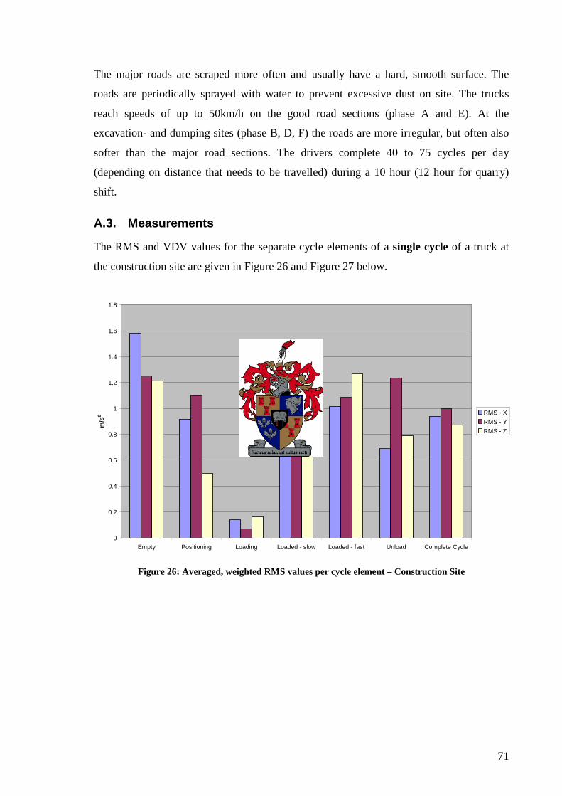
71
The major roads are scraped more often and usually have a hard, smooth surface. The
roads are periodically sprayed with water to prevent excessive dust on site. The trucks
reach speeds of up to 50km/h on the good road sections (phase A and E). At the
excavation- and dumping sites (phase B, D, F) the roads are more irregular, but often also
softer than the major road sections. The drivers complete 40 to 75 cycles per day
(depending on distance that needs to be travelled) during a 10 hour (12 hour for quarry)
shift.
A.3. Measurements
The RMS and VDV values for the separate cycle elements of a single cycle of a truck at
the construction site are given in Figure 26 and Figure 27 below.
0
0.2
0.4
0.6
0.8
1
1.2
1.4
1.6
1.8
Empty Positioning Loading Loaded - slow Loaded - fast Unload Complete Cycle
m/s
2 RMS - X
RMS - Y
RMS - Z
Figure 26: Averaged, weighted RMS values per cycle element – Construction Site

72
0
1
2
3
4
5
6
7
8
Empty Positioning Loading Loaded - slow Loaded - fast Unload Complete Cycle
m/s
1.75 VDV - X
VDV - Y
VDV - Z
Figure 27: Weighted VDV values per cycle element – Construction Site
From both figures it is evident that the WBV level is highest while the truck is empty. The
hard suspension and relative low mass causes the truck to jump around while empty. The
vibrations in all directions are fairly high, but this is mainly due to high driving speed. The
x-direction is prominent, but this could be attributed to driving technique. The rear
suspension, not carrying any load, is very stiff and consequently bounces more than the
front suspension, causing a pivoting motion of the cab. This results in backslapping by the
backrest, leading to the driver being unable to maintain a constant depression of the
accelerator pedal. The truck jerks as a result, contributing to the high longitudinal
vibration.
Positioning the truck for the load involves driving over very irregular terrain at low speed.
This is seen in the VDV graph, since many peaks will cause the VDV to climb faster than
the RMS. The truck is articulating sharply during this period (sometimes the cab is moved
by the hydraulic steering mechanism while the truck is stationary to provide space for other
trucks) and the transverse and longitudinal directions recorded high values. Rolling of the
cab as the vehicle traverses large obstacles with almost no correlation between left and
right tire inputs also contribute to the high transverse measurements.

73
The loading period consists of peaks followed by waiting periods and thus the VDV values
climb much faster than the RMS values. The values obtained depend on how the load is
placed as well as the size of the load. Some loaders “place” the load on the bin, while
others “drop” the load on the bin. Some loaders load 10 tons at a time (which may contain
giant boulders) while others load only 5 tons at a time. The y-direction may have a high
value when the driver straightens out the truck during loading (the front chassis articulates
behind the cab, thus when the hydraulic pistons steer the chassis, the cab moves sideways
dragging the wheels slightly as it yaws) for a quicker exit.
Once loaded, the truck needs to traverse the rough terrain before joining the main road.
This is usually done at low speed. Sometimes the terrain is fairly soft and will give way
under the truck (such as at the slipway), but sometimes the terrain is very hard leading to
high values in all directions (such as in the burrow pit). Vibrations in all directions are very
similar.
When the loaded truck reaches the maintained road the driver starts to speed up. Here the
transverse and longitudinal vibrations are less than the vertical direction, but the values are
dependent on the severity of road irregularities.
Approaching the dumping site, the terrain starts to deteriorate again. The truck slows down
and articulates a lot during this time causing lateral vibrations to increase. Unloading only
takes a couple of seconds, but is dominated by lots of peaks as large rocks fall off the back.
As the bin is lowered and impacts the rear chassis an impulse is recorded on the driver’s
seat in the vertical direction, hence the high VDV value in the vertical direction.
It is interesting to note that, for the complete cycle, the lateral direction has the highest
exposure levels for RMS and VDV.
RMS and VDV values for the separate cycle elements of a single cycle of a truck at the
quarry are given in Figure 28 and Figure 29 below.

74
0
0.2
0.4
0.6
0.8
1
1.2
1.4
Empty Positioning Loading Loaded - slow Loaded - fast Unload Complete Cycle
m/s
2
RMS - X
RMS - Y
RMS - Z
Figure 28: Average, weighted RMS values per cycle element - Quarry
0
0.5
1
1.5
2
2.5
3
3.5
4
4.5
Empty Positioning Loading Loaded - slow Loaded - fast Unload Complete Cycle
m/s
1.75 VDV - X
VDV - Y
VDV - Z
Figure 29: Weighted VDV values per cycle element - Quarry
The figures show that the WBV is highest when the truck is loaded and driving slowly near
the loading spot. The vibration is the highest in the z-direction. The highest vibration in the
x-direction is perceived while driving the empty truck from the dumping site to the loading
site. The vibration in the y-direction is the highest during positioning.
75
Positioning the truck for the load involves driving over very irregular terrain at low speed.
This is seen in the VDV graph, since many peaks will cause the VDV to climb faster than
the RMS. Since the truck is articulating sharply during this period (there is little space to
turn and position the truck next to the excavator), the transverse and longitudinal directions
recorded high values.
The loading period consists of peaks followed by waiting periods and thus the VDV values
climb much faster than the RMS values. After each cycle, the driver picks up a notepad
from the dash board to make notes of the previous cycle and puts it back near the
windscreen. During this manoeuvre, the driver is getting up from and falling back into the
seat twice. The vibrations during loading are not only caused by the load dropping in the
bin, but mainly by the driver himself (also observed by Newell, 2004).
Once loaded, the truck needs to traverse the rough terrain before joining the road down the
hill. This is usually done at a low speed. In this area, the holes and bumps in the road are
the most severe. Vibrations in all directions are very similar.
When the loaded truck reaches the maintained road the driver starts to speed up. During
this part of the cycle, the vibrations are less and almost no shocks occur.
Approaching the dumping site, the terrain starts to deteriorate again. The truck slows down
and articulates a lot during this time pushing the lateral vibrations up. The unloading is
quite quick, but is dominated by lots of peaks as large rocks fall off the back. The bin itself
causes vertical vibrations when lowered.
Over the complete cycle it is seen that while the vertical direction has the highest RMS
vibration exposures level, it is the lateral direction that has the highest VDV vibration
exposure level (just as at the construction site).
A.4. Comparison
From the figures given above it may be seen that the levels at the construction site is much
higher than that at the quarry. This is mainly due to better road surfaces at the quarry,
inducing smaller vibration inputs to the truck through the wheels. It is also seen that for

76
both scenarios the vibration exposure levels are high in all directions when the truck is
empty and travelling at high speeds. It is also clearly seen that the vertical direction is not
the worst axis for most of the cycle elements, as is so commonly assumed when designing
suspensions. The lateral direction is the worst when there is poor correlation between the
left and right wheel inputs (poor road surfaces) and the longitudinal axis is the worst axis
when the truck is empty and travelling at high speed.
A.5. Exposure
The measurements above were representative of a single cycle. The drivers at the
construction site work 10 hour shifts and aim to complete between 40 and 60 cycles
depending on the distance travelled per cycle. At the time taken to complete one cycle, as
recorded above, 40 cycles would be completed in 10 hours. The drivers at the quarry work
12 hour shifts and aim to complete up to 75 cycles depending on the distance travelled per
cycle. With the cycle time that was accomplished during the measurements, there would be
73 cycles in the 12 hour working day.
Both drivers were approximately 1.75m tall and weighed 80kg - 90kg. It is evident from
the figures above that the driving style has a large influence on the exposure levels. If the
driver were to drive slower, or, not turn the cab while the truck is stationary, the exposure
levels will be reduced.
Each cycle element of the comparison measurements takes 1 - 3 min, bringing a complete
cycle to ±14 min. In Table 1 and 2 below the WBV exposure and calculations are recorded
for an equivalent 8 hour day. Each recorded exposure represents a different element of the
cycle as explained above. The “partial” values in the first two columns are the 8 hour
equivalent values calculated from the measured values and time of exposure. The “Time to
reach” columns indicate the time in hours and minutes (up to 24 hrs) it would take (at that
vibration magnitude) to reach the EAV or ELV. The “Total exposure” columns are
calculated from the “partial” values and thus represent the equivalent exposure for 8 hours.
The 10- and 12 hour exposures are thus bunched into 8 hours, to get an 8-hour equivalent
exposure.

77
It has been shown by the HSE that for durations of exposure less than 8 hours, the RMS is
more lenient, while for exposures of more than 8 hours, the VDV is more lenient (provided
there are not too many peaks) (HSE, 2004).
For the construction site, in a 10 hour day, the driver would spend only 100 minutes on
each of the 6 cycle elements and thus, when calculating the time (for each element) to
reach EAV, the RMS will be more lenient than the VDV (as each exposure is less than 8
hours) As a whole, however, the driver is exposed to more than 8 hours of vibration, thus
the total VDV will be more lenient than the total RMS and we find that the RMS exceeds
the ELV (1.42 m/s2), while the VDV (20.8 m/s1.75) does not. At the quarry, the exposure
times are slightly longer, but the levels much lower. The daily exposure values that are
calculated by the HSE calculator are 0.72 m/s2 en 14.5 m/s1.75.
A.6. Conclusions
At present the EU-Directive does not stipulate whether the VDV or RMS values should be
used to determine whether the EAV or ELV have been exceeded. It can thus be concluded,
if the VDV total is used that, although the EAV is exceeded, the drivers are not exceeding
the ELV. The measurements, however, show that they are very close to the limit and action
should be taken to reduce the exposure levels at both sites.
The exposure levels could be reduced in various ways, but one of the easiest ways would
be to educate the drivers of the consequences of their driving styles. Changing the driving
style slightly (such as not turning while stationary) would not influence production
efficiency much, yet reduce the vibration exposure. It was noticed that the trucks often wait
for the excavator to load other trucks before being loaded themselves. If the driver were to
drive slower, the vibration exposure levels and the waiting time will be reduced.
It was seen that the highest exposure levels occur when the truck is empty (at the
construction site) and when the truck is full (at the quarry) and the lowest levels occur
when the truck is being loaded. Attention should be given to improving the suspension for
ride during the hauling periods. The suspension seat should also be adjusted correctly for
the driver to reduce the vibration exposure levels.
78
It has been shown that vibration along all three axes (x, y and z) should be considered and
not only the vertical axis. The condition of the road plays a vital role in vibration exposure
and care should be taken to keep the road smooth and hard at all times.
Rimell and Mansfield (2004) investigated the difference in vibration exposure levels
between two ADTs operating in a quarry. The one ADT had a normal steel bin (hopper)
while the other ADT had a rubber-lined bin (hopper). They discovered that, although the
rubber lining did not contribute much to the attenuation of vibration exposure levels during
the hauling periods, it attenuated the vibration exposure levels during the loading,
unloading and positioning periods. Once the suspension systems are optimised for the
hauling periods, a solution such as this may be introduced to improve ride comfort during
the other phases as well.

79
Table 13: WBV exposure as calculated by HSE calculator for construction site
Table 14: WBV exposure as calculated by HSE calculator for quarry
Partial Partial Time to reach EAV Time to reach EAV Time to reach ELV Total Total
VDV exposure (VDV option) (A(8) option) (A(8) option only) VDV exposure
m/s 1.75 m/s² A(8) 9.1 m/s 1.75 VDV
0.5 m/s 2 A(8)
1.15 m/s 2 A(8)
m/s 1.75 m/s² A(8) hours minutes hours minutes hours minutes
Empty 15.9 0.72 0 11 0 48 4 14 20.8 1.42 Positioning 15.1 0.50 0 13 1 39 8 42
Loading 3.0 0.07 >24 0 >24 0 >24 0
Loaded - slow 9.8 0.35 1 14 3 23 17 56
Loaded - fast 11.6 0.89 0 38 0 32 2 47
Unloading 14.5 0.56 0 16 1 19 6 58
Partial Partial Time to reach EAV Time to reach EAV Time to reach ELV Total Total
VDV exposure (VDV option) (A(8) option) (A(8) option only) VDV exposure
m/s 1.75 m/s² A(8) 9.1 m/s 1.75 VDV
0.5 m/s 2 A(8)
1.15 m/s 2 A(8)
m/s 1.75 m/s² A(8)
hours minutes hours minutes hours minutes
Empty 9.8 0.39 1 31 3 17 17 21 14.5 0.72 Positioning 10.7 0.33 1 3 4 31 23 51
Loading 4.9 0.08 23 11 >24 0 >24 0
Loaded - slow 11.9 0.44 0 40 2 35 13 40
Loaded - fast 8.6 0.32 2 28 5 2 >24 0
Unloading 6.6 0.05 7 9 >24 0 >24 0

80
Appendix B: Theoretically Perfect Isolation
Theoretically it is possible to completely isolate the driver from any vibration exposure.
Assume the truck could be represented by a 2D rigid body with 3 force inputs (one at each
axle). It is possible for the body to be in force and moment equilibrium, however, because
the system is statically indeterminate, it is not possible to solve for the forces explicitly, but
only for 2 of the forces in terms of the third. If, Ff, is specified, then the condition for
equilibrium is,
fr
r Fd
LF =1 ( 15 )
and,
fr
r Fd
LF )1(2 −= ( 16 )
where L is the distance between the front and rear most force, and dr is the distance
between the two rear forces. If we imagine the forces to be due to springs with
displacement inputs at their bases and that the input displacements are of equal amplitude
and properly phased, then if the spring constants are distributed according to,
fr
r kd
Lk )(1 = ( 17 )
and,
fr
r kd
Lk )1(2 −= ( 18 )
the rigid body would be perfectly isolated from the input. This means that although the
bases of the springs are all being driven, the body would be perfectly still.
The input phasing that would produce this occurrence is shown in Figure 30. If the
roadway were distributed such that the steer axle and rear live axle were in phase while the
front live axle was out of phase, and the springs were distributed as stated, then the rigid
body would roll along the roadway and experience no accelerations at all. Interestingly, the

81
very road that results from the truck driving over it has exactly this distribution (Margolis,
2001).
Figure 30: Roadway profile for isolation of beaming (Margolis, 2001)
For most trucks the quantity L/dr, is about 4 and, L/dr – l, is 3. This means that the front
live axle must be 4 times stiffer than the steer axle and the rear live axle must be 3 times
stiffer.
It must be remembered that the prescribed suspension parameter distribution is only for
rigid body isolation from the prescribed roadway. If such a roadway existed, and a truck
sat upon this roadway with the required configuration, then the truck will always be in this
configuration regardless of speed. Thus the rigid body isolation would take place for all
forward speeds, which translates into all frequencies.
dr L

82
Appendix C: MATLAB Simulation Models:
The MATLAB simulation models were developed by first setting up the equations of
motion by applying Newton II and then rewriting them in matrix form:
FxKxCxM =++ &&& ( 19 )
where:
M = n x n diagonal mass-and-inertia-matrix
C = n x n symmetrical damping-matrix
K = n x n symmetrical stiffness-matrix
F = n x 1 vector of forcing functions created by road
x = n x 1 vector of responses
n = number of degrees of freedom
If the damping matrix, C, is not proportional, (that is C ≠ αK + βM, where α and β are
constants) then the problem may be solved using the state space formulation with a
numerical integration method (such as the Runga Kutta function ode45) in MATLAB. The
equation of motion becomes:
+
−−=
−−− FMx
x
CMKM
I
x
x111
00&&&
&
( 20 )
Solving the equation with ode45 in MATLAB will produce answers for velocity and
displacements, but not acceleration. The acceleration may be approximated by using
Euler’s algorithm.
If the damping matrix, C, is proportional (that is C = αK + βM, where α and β are
constants) then the problem may be uncoupled into n single degree of freedom problems
and thus could be solved using any method applicable to single degree of freedom systems.
It must, however, be noted that vehicle suspension generally do not have proportional
damping.

83
Assume
yUx = ( 21 )
KMC βα += ( 22 )
Then:
FUxKUUxCUUxMUU TTTT =++ &&& ( 23 )
FyKyCyM ˆˆˆˆ =++ &&& ( 24 )
where U is the matrix with the eigenvectors of the undamped system as columns and M ,
C and K are uncoupled diagonal matrices. Solving each y is as easy as solving a single
degree of freedom system for which the solution is known.
C.1. 2 Dimensional, 4-DOF Model: The first MATLAB model is a simplification of the real truck. The truck was essentially
divided into two parts, namely the chassis and the walking beams. Each part having 2
degrees of freedom (pitch and bounce). The tires and struts were added in series to model
the front suspension and the tires and sandwich blocks were added in series to model the
rear suspension. Figure 31 shows the graphical representation of what the first MATLAB
model simulated.
Figure 31: First 2D MATLAB model
C.2. 2 Dimensional, 7-DOF Model:
The first MATLAB model was upgraded to 7 degrees-of-freedom (shown in Figure 32).
The main differences being that the cab and the bin were modelled as separate rigid bodies.
The cab was allowed to pitch and bounce independently from the chassis, while the bin
could only bounce and not pitch relative to the chassis.

84
Figure 32: Second 2D MATLAB model
C.3. 3 Dimensional, 15-DOF Model:
A 3 dimensional model of the truck was created in MATLAB. The difference between a 2
dimensional and 3 dimensional model is the planes in which it can move. The 2
dimensional could not roll or displace in the lateral direction. The 3 dimensional model,
however, is able to move and rotate about all three the major axes. The model developed in
MATLAB was based on the 7-DOF model, but given more degrees of freedom by
allowing roll motions of the chassis, cab and bin. A simplified seat model was also
included in the model. The 15 degrees-of-freedom MATLAB model is shown in Figure 33.
Figure 33: 3D MATLAB model - a) Side view, b) Front view
For clarity Table 3: Degrees-of-freedom of MATLAB models is repeated below.
b) a)

85
Table 15: Degrees-of-freedom of MATLAB models
2 Dimensional 4 degree-of-freedom model
2 Dimensional 7 degree-of-freedom model
3 Dimensional 15 degree-of-freedom model
Vertical displacement:
• Chassis • Walking beam
Angular displacement about
y-axis (pitch):
• Chassis • Walking beam
Vertical displacement:
• Chassis • Walking beam • Cabin • Bin
Angular displacement about
y-axis (pitch):
• Chassis • Walking beam • Cabin
Vertical displacement:
• Chassis • Two walking beams • Cabin • Bin • Seat
Angular displacement about
y-axis (pitch):
• Chassis • Two walking beams • Cabin • Bin
Angular displacement about
x-axis (roll):
• Front chassis • Rear chassis • Cabin • Bin

86
Appendix D: Beaming From the literature review it was seen that certain vibrations may be generated by the
bending vibration of the chassis, commonly known as beaming. Ibrahim et al. (1994)
developed a model to investigate the effect of a flexible frame on ride vibration in large
trucks. He concluded that frame flexibility may contribute significantly to vibration
measurements, especially on the trailer. In his article Donald Margolis (2001) stated that
the rigid body modes of a truck are most important at frequencies below 5Hz, while
beaming occurs close to the wheel-hop frequency at about 10Hz.
The beaming frequency of the ADT’s chassis may be determined by approximating the
rear chassis as a beam that has a large inertia at the one end (representing the cabin) and a
added inertia at specified points along its length (representing the bin). The beam is
connected to a fixed plane (the road) via springs (representing the front and rear suspension
components) at specified points along its length. The approximations are shown in Figure
34 below. The nodes are numbered 1 – 5. The “m” represents added inertia from bin and
load; the “M” represents the added inertia of the cab and front chassis. The dashed vertical
lines represents the spring-characteristics of the front and rear suspension. The dash-dotted
line shows the first mode-shape of the transverse vibration at the frequency of interest.
Figure 34: Chassis beaming simplification
Two techniques (Finite Elements and Bernoulli as described in sections 6.5 and 8.3 of
Inman, 2001) were used to determine the natural frequency of the transverse vibration of
the chassis. Both techniques gave a beaming mode at about 11.8Hz for the loaded truck
5 4 3 2 1
m m m M

87
and a beaming mode at 22Hz for the unloaded truck. This correlates quite well with the
10Hz predicted by Margolis (2001).
Studying Figure 34, it may be seen that beaming is difficult to control from the suspension
locations, as the shock absorbers do little to extract energy from the beaming mode. The
primary suspension can, however, be used to control the rigid body modes. If beaming is
excited, it should be dealt with through cab isolation techniques.
The beaming of the chassis was not considered in the optimisation study. The beaming
mode of interest does not contribute significantly to vertical vibrations at the cabin (see
Figure 34) and is at too high a frequency to contribute significantly to the horizontal
vibrations (see Wd filter in Figure 17), especially for the unloaded condition.