Uncalibrated Neural Inverse Rendering for Photometric Stereo of GeneralSurfaces

Berk Kaya1 Suryansh Kumar1 Carlos Oliveira1 Vittorio Ferrari2 Luc Van Gool1,3

Computer Vision Lab, ETH Zurich1, Google Research2, KU Leuven3

Abstract

This paper presents an uncalibrated deep neural networkframework for the photometric stereo problem. For trainingmodels to solve the problem, existing neural network-basedmethods either require exact light directions or ground-truth surface normals of the object or both. However, inpractice, it is challenging to procure both of this informa-tion precisely, which restricts the broader adoption of pho-tometric stereo algorithms for vision application. To bypassthis difficulty, we propose an uncalibrated neural inverserendering approach to this problem. Our method first es-timates the light directions from the input images and thenoptimizes an image reconstruction loss to calculate the sur-face normals, bidirectional reflectance distribution functionvalue, and depth. Additionally, our formulation explicitlymodels the concave and convex parts of a complex surfaceto consider the effects of interreflections in the image forma-tion process. Extensive evaluation of the proposed methodon the challenging subjects generally shows comparable orbetter results than the supervised and classical approaches.

1. IntroductionSince Woodham’s seminal work [69], the photometric

stereo problem has become a popular choice to estimate anobject’s surface normals from its light varying images. Theformulation proposed in that paper assumes the Lambertianreflectance model of the object, and therefore, it does notapply to general objects with unknown reflectance property.While multiple-view geometry methods exist to achieve asimilar goal [57, 20, 70, 76, 35, 24, 36, 37], photometricstereo is excellent at recovering fine details on the surface,like indentations, imprints, and even scratches. Of course,the solution proposed in Woodham’s paper has some unre-alistic assumptions. Still, it is central to the development ofseveral robust algorithms [71, 30, 55, 1, 22, 26] and also liesat the core of the current state-of-the-art deep photometricstereo methods [28, 65, 12, 10, 11, 42, 41, 27].

Generally, deep learning-based photometric stereo meth-ods assume a calibrated setting, where all the light source

information is given both at the train and test time [28, 56,12, 65]. Such methods attempt to learn an explicit relationbetween the reflectance map and the ground-truth surfacenormals. But, the exact estimation of light directions is a te-dious process and requires expert skill for calibration. Mo-tivated by that, Chen et al. [10, 11] recently proposed an un-calibrated photometric stereo method. Though it estimateslight directions using image data, the proposed method re-quires ground-truth surface normals for training the neuralnetwork. Certainly, procuring ground-truth 3D surface ge-ometry is difficult, if not impossible, which makes the ac-quisition task of correct surface normals strenuous. For 3Ddata acquisition, active sensors are mostly used, which isexpensive and often needs post-processing of the data to re-move noise and outliers. Hence, the necessity of ground-truth surface normals limits the usage of such an approach.

Further, most photometric stereo methods, including cur-rent deep-learning methods, assume that each surface pointis illuminated only by the light source, which generallyholds for a convex surface [49]. However, objects, mainlyfrom ancient architectures, have complex geometric struc-tures, where the shape may compose of convex, concave,and other fine geometric primitives (see Fig.1(a)). Whenilluminated under a varying light source, certain concaveparts of the surface might reflect light onto other parts ofthe object, depending on its position. Surprisingly, this phe-nomenon of interreflections is often ignored in the modelingand formulation of a photometric stereo problem, despite itsvital role in the object’s imaging [28, 65, 12, 10, 11].

In this work, we overcome the above shortcomings byproposing an uncalibrated neural inverse rendering network.We first estimate all the light source directions and intensi-ties using image data. Computed light source informationis then fed into the proposed neural inverse rendering net-work to estimate the surface normals. The idea is, those cor-rect surface normals, when provided to the rendering equa-tion, should reconstruct the input image as close as possi-ble. Consequently, we can bypass the requirement of theground-truth surface normals at train time. Unlike recentmethods, we model the effects of both the light source andthe interreflections for rendering the image. Although one

arX

iv:2

012.

0677

7v3

[cs

.CV

] 1

7 A

pr 2

021

Incident Ray from the Source

on the Concave Region

Incident Ray from the Source

on the Convex Region

Illuminates the other surface element.

Com

pone

nt o

f lig

ht In

tens

ity

rece

ived

at th

e Sen

sor d

ue to

th

e sec

onda

ry so

urce

Inte

nsity

rece

ived

at th

e Sen

sor

due t

o th

e prim

ary

sour

ce

Light Source

Light Source

Camera

(a) Photometric Stereo Setup

Woodham (1980)MAE = 30.66°

Nayar et al. (1991)MAE = 28.82°

Taniai et al. (2018)MAE = 23.97°

OursMAE = 19.91°

Chen et al. (2020)MAE = 49.36°

Ikehata (2018)MAE = 34.00°

(b) Qualitative and Quantitative Comparison

Figure 1: (a) Example showing the interreflection effect due to concave geometric structure. The light from the primary source hits the concave regionof the surface that illuminates the other surface points which then act as a secondary light source. (b) Comparison of our approach against the classical anddeep-learning methods on the Vase dataset which shows that it performs better than others. We used Mean Angular Error (MAE) metric to report the results.

can handle interreflection using classical methods [49, 9],the reflectance characteristics of different types of materialare quite diverse. Hence, we want to leverage neural net-work’s powerful capability to learn complex reflectance be-havior from the input image data.

For evaluation, we performed experiments on DiLiGenTdataset [62]. We noticed that the objects present with thisdataset are not apt for studying interreflections. To that end,we proposed a novel dataset to study the behavior and effectof interreflections on the object’s imaging §5. We observedthat ignoring interreflections can dramatically affect the ac-curacy of the surface normals estimate (see Fig 1(b)). Tosum up, our paper makes the following contributions:• This paper presents an uncalibrated deep photometric

stereo method that does not require ground-truth surfacenormals at train time to solve photometric stereo.

• Our work considers the contribution of both the sourcelight and interreflections in the image formation process.Consequently, our approach is more general and applica-ble to a wide range of objects.

• The proposed method leverages neural inverse renderingprinciples to infer the surface normals, depth, and spa-tially varying bidirectional reflectance distribution func-tion (BRDF) values from input images. Our method gen-erally provides comparable or better results than the clas-sical [49, 2, 60, 73, 45, 52, 44] and the recent superviseduncalibrated deep learning methods [12, 15, 11].

2. Related WorkFor comprehensive review on photometric stereo readers

may refer to Herbort et al. [25], and Chen et al. [11] work.

1. Calibrated Photometric Stereo. The methods pro-posed under this setting assume that all the light source in-formation is known for computing surface normals. Sev-

eral calibrated methods have been proposed to handle non-Lambertian surfaces [48, 72, 71, 47, 50, 31]. These methodsassume non-Lambertian effects, such as specularities, aresparse and confined to a local region of the surface. So, theyfilter them before computing surface normals. For exam-ple, Wu et al. [71] proposed a rank minimization approachto robustify photometric stereo. Oh et al. [50] introduceda partial sum of singular values optimization algorithm forthe low-rank normal matrix recovery. Other popular outlierrejection methods were based on RANSAC [48], Bayesianregression [30, 31], and expectation-maximization [72].

With the recent success of deep learning in many com-puter vision areas, several learning-based approaches havealso emerged for the photometric stereo problem. Santoet al. [56] introduced a deep photometric stereo network(DPSN) that learns the mapping between the surface nor-mals and the reflectance map. Ikehata [28] merged all pixel-wise information to an observation map and trained a net-work to perform per-pixel estimation of normals. In con-trast, Taniai et al. [65] used a self-supervised frameworkto recover surface normals from input images. Yet, it usesthe classical photometric equation that fails to model inter-reflections. Moreover, it uses Woodham’s method [69] toinitialize the surface normals in their loss function whichis not robust, and therefore, their trained network model issusceptible to noise and outliers.

2. Uncalibrated Photometric Stereo. These methods as-sume unknown light source information for solving photo-metric stereo. However, not knowing the light sources leadsto an ambiguity i.e., there exists a set of surfaces under un-known distant light sources that can lead to identical im-ages. Hence, the actual surface can be recovered up to athree-parameter ambiguity popularly known as GeneralizedBas-Relief (GBR) ambiguity [5, 9]. Existing methods elim-

inate this ambiguity by making some additional assump-tions in their proposed solution. Alldrin et al. [2] assumesbounded values on the GBR variables and resolves the am-biguity by minimizing the entropy of albedo distribution.Shi et al. [60] assumes at least four pixels with different nor-mals but the same albedo. Papadhimitri et al. [52] presentsa closed-form solution by detecting local diffuse reflectancemaxima (LDR). Other methods assume perspective projec-tion [51], specularities [21, 18], low-rank [59], interreflec-tions [9] or symmetry properties of BRDFs [64, 73, 44].

Apart from the traditional methods, Chen et al. [12] pro-posed a learning framework (UPS-FCN). This method by-passes the light estimation process and learns a direct map-ping between the image and the surface normal. But, theknowledge of the light source would provide useful evi-dence about the surface normals, and therefore completelyignoring the light source data seems implausible. The self-calibrating deep photometric stereo networks work [10] re-cently introduced an initial lighting estimation stage (LC-Net) from images to overcome the problem with UPS-FCN.Recently, Chen et al. [13] also proposed a guided calibra-tion network (GCNet) to overcome the limitations of LC-Net. Unlike existing uncalibrated deep-learning methodsthat rely heavily on ground-truth surface normals for train-ing, our method can solve photometric stereo by using animage reconstruction term as a function of estimated sur-face normals. The goal is to let the network learn the imageformation process and the complex reflectance model of theobject via explicit interreflection modeling.

3. Photometric StereoPhotometric stereo aims to recover the surface normals

of an object from its multiple images captured under vary-ing light illuminations. It assumes a unique point lightsource per image taken by a camera from a constant viewdirection v which is commonly assumed to be at (0, 0, 1)T .Under such configuration, when a surface point x is il-luminated by a distant point light source from direction‘ls ∈ R3×1’, the image intensity Xs(x) measured by thecamera due to sth source in the view direction v is given by

Xs(x) = es · ρ(n(x), ls,v

)· ζa(n(x), ls

)· ζc(x) (1)

Here, the camera projection model is assumed to be or-thographic. The function ρ(n(x), ls,v) gives the BRDFvalue, ζa(n(x), ls) = max(n(x)T ls, 0) accounts for theattached shadow, and ζc(x) ∈ 0, 1 assign 0 or 1 valueto x depending on whether it lies in the cast shadow regionor not. es ∈ R+ is a scalar for light intensity value, andn(x) ∈ R3×1 is the surface normal vector at point x. Eq:(1)is most-widely used photometric stereo formulation whichgenerally works well in practise [9, 30, 28, 65, 13, 11].1. Classical Photometric Stereo Model. It assumes aconvex Lambertian surface model resulting in a constant

BRDF value across the whole surface. Additionally, thesurface is considered to be illuminated only due to the lightsource. Under such assumptions, Eq:(1) becomes a lin-early tractable problem and it is possible to recover the sur-face normals by solving a simple system of linear equa-tions. Let all the n light source directions be denoted asL = [l1, l2, .., ln] ∈ R3×n and m unknown surface pointnormal be N = [n(x1),n(x2), ..,n(xm)] ∈ R3×m. Usingthe notation, we can write Eq:(1) due to all the light sourcesand surface points compactly as

Xs = ρNTL (2)

where, Xs ∈ Rm×n is the matrix consisting of n imageswithm object pixels stacked as column vectors, and ρ is theconstant albedo. The above system can be solved for thesurface normals using the matrix pseudo-inverse approachunder calibrated setting if n ≥ 3 (i.e., at least three lightsources are given in non-degenerate configuration).2. Interreflection Model. In contrast to the classical pho-tometric stereo, here, the total radiance at a point x on thesurface is the sum of radiance due to light source s and theradiance due to interreflection from other surface points.

X(x) =

due to light source︷ ︸︸ ︷Xs(x) +

due to interreflections︷ ︸︸ ︷ρ(x)

π

∫Ω

K(x,x′)X(x′)dx′(3)

where, Ω represents the surface, x′ is another surface point,and dx′ the differential surface element at x′. The value ofthe interreflection kernel ‘K’ at x due to x′ is defined as:

K(x,x′) =( (n(x)T (−r)) · (n(x′)T r) · V (x,x′)

(rT r)2

)(4)

The values of K, when measured for each surface el-ement form a symmetric and positive semi-definite matrix.In Eq:(4), V (x,x′) captures the visibility. When x occludesx′ or vice-versa then V is 0. Otherwise, V gives the orienta-tion between the two points using the following expression:

V (x,x′) =(n(x)T (−r) + |n(x)T (−r)|

2|n(x)T (−r)|

)·(n(x′)T r + |n(x′)T r|

2|n(x′)T r|

) (5)

where, n(x) and n(x′) are the surface normal at x and x′,and r = x−x′ is the vector from x′ to x. Substituting V andK in Eq:(3) gives an infinite sum over every infinitesimallysmall surface element (point) and therefore, it is not compu-tationally easy to find a solution to X(x) in its continuousform. Nevertheless, the solution to Eq:(3) is guaranteed toconverge as ρ(x) < 1 for a real surface. To practicallyimplement the interreflection model, the object surface is

discretized into m facets [49]. Assuming the radiance andalbedo values to be constant within each facet, then Eq:(3)for the ith facet becomesXi = Xsi+

ρiπ

∑mj=1, j 6=iXjKij ,

where Xi ∈ Rn×1 and ρi are the radiance and albedo offacet i. Considering the contribution of all the light sourcesfor each facet, it can be compactly re-written as:

X = Xs + PKX, ⇒ X = (I−PK)−1Xs (6)

where, X = [X1, X2, ., Xm]T is the total radiance for allthe facets, and Xs = [Xs1, Xs2, ., Xsm]T is the light sourcecontribution to the radiance of m facets. Furthermore, Pis a diagonal matrix composed of albedo values and K isa m × m interreflection kernel matrix with diag(K) = 0.Nayar et al. [49] proposed Eq:(20) to recover the surfacenormals for concave objects. The algorithm proposed toestimate surface normals using Eq:(20) first computes thepseudo surface normals by treating the object as directly il-luminated by light sources. These pseudo surface normalsare then used to iteratively update for the interreflection ker-nel and surface normals via depth map estimation step, untilconvergence. In the later part of the paper, we denote thenormals estimated using Eq:(20) as Nny . The Nayar’s in-terreflection model assumes Lambertian surfaces and over-looks surfaces with unknown non-Lambertian properties.

4. Proposed MethodGiven X = [X1, X2, ..., Xn] a set of n input images and

the object mask O, we propose an uncalibrated photomet-ric stereo method to estimate surface normals. Here, eachimage Xi is reshaped as a column vector and not a facetsymbol as used in interreflection modeling. Even though theproblem with unknown light directions gives rise to the bas-relief ambiguity [5], we leverage the potential of the deepneural networks to learn those source directions from theinput image data using a light estimation network §4.1. Theestimated light directions are used by the inverse renderingnetwork §4.2 to infer the unknown BRDFs and surface nor-mals using our proposed rendering equation. Our renderingapproach explicitly utilizes the role of the light source andinterreflections in the image reconstruction process.

4.1. Light Estimation Network

Given X and O, the light estimation network predictsthe light source intensities (ei’s) and direction vectors (li’s).We can train such a network either by regressing the inten-sity values and the corresponding unit vector in the source’sdirection or classifying intensity values into pre-definedangle-range bins. The latter choice seems reasonable as it iseasier than regressing the exact direction and intensity val-ues. Further, quantizing the continuous space of directionsand intensities for classification makes the network robust to

𝜃

𝜙

li

(a) Source Discretization

li

no(x)

rxi

v

x

𝜃𝜃

(b) Surface Reflectance

Figure 2: (a) The estimated source directions are given by two param-eters: φ ∈ [0, π] and θ ∈ [−π/2, π/2]. (b) Illustration of surface re-flectance. When light ray li hits a surface element, the specular componentalong the view-direction of the point x due to ith source is given by rxi.Figure 2(b) geometry presentation is inspired by Keenan work [17].

small changes due to outliers or noise. Following that, weexpress the light source directions in the range φ ∈ [0, π]for azimuth angles and θ ∈ [−π/2, π/2] for elevation an-gles (Fig.2(a)). We divide the azimuth and elevation spacesinto Kd = 36 classes. We classify azimuth and elevationseparately, which reduces the problem’s dimensionality andleads to efficient computation. Similarly, we divide the lightintensity range [0.2, 2.0] into Ke = 20 classes [10].

We used seven feature extraction layers to extract imagefeatures for each input image separately, where each layerapplies 3 × 3 convolution and LReLU activation [74]. Theweights of the feature extraction layers are shared amongall the input images. However, single image features cannotcompletely disambiguate the object geometry with the lightsource information. Therefore, we utilize multiple imagesto have a global implicit knowledge about the surface’s ge-ometry and its reflectance property. We use image specificlocal features and combine them using a fusion layer to geta global representation of the image set via a max-poolingoperation (Fig.3). The global feature representation with theimage-specific features is then fed to a classifier. The classi-fier applies four layers of 3×3 convolution and LReLU acti-vation [74] as well as two fully-connected layers to provideoutput softmax probability vectors for azimuth (Kd), ele-vation (Kd), and intensity (Ke). Similar to the feature ex-traction, the classifier weights are shared among each other.The output value with maximum probability is convertedinto a light direction vector li and scalar intensity ei.Loss function for Light Estimation Network. The lightestimation network is trained using a multi-class cross-entropy loss [10]. The total calibration loss Lcalib is:

Lcalib = Laz + Lel + Lin (7)

Here Laz , Lel, and Lin are the loss terms for azimuth,elevation, and intensity respectively. We used syntheticBlobby and Sculpture datasets [12] to train the network.The light source labels from these datasets are used for su-pervision at the train time. The network is trained using theabove loss for once and the same network is used at the testtime for all other datasets §5.

4.2. Inverse Rendering Network

To estimate an object surface normals from X, we lever-age neural networks’ powerful capability to learn from data.The prime reason for that is, it is difficult to mathemati-cally model the broad classes of BRDFs without any priorassumptions about the reflectance model [21, 16, 22]. Al-though there are methods to estimate BRDF values using itsisotropic and low-frequency property [29, 61], it prohibitsthe modeling of unrestricted reflectance behavior of the ma-terial. Instead of such explicit modeling, we build on theidea of neural inverse rendering [65], where the BRDFs andsurface normals are predicted during the image reconstruc-tion process by the neural network. We go beyond Taniaiet al. [65] work by proposing an inverse rendering networkthat synthesizes the input images using a rendering equationthat explicitly uses interreflections to infer surface normals.(a) Surface Normal Modeling. We first convert X intoa tensor X ∈ Rh×w×nc, where h × w denote the spatialdimensions, n is the number of images, and c is the numberof color channels (c = 1 for grayscale and c = 3 for colorimages). X is then mapped to a global feature map Φ asfollows:

Φ = ξf (X ,O,Θf ) (8)

O is used to separate the object information from the back-ground. ξf is a three layer feed-forward convolutional net-work with learnable parameter Θf . Each layer applies 3×3convolution, batch-normalization [32] and ReLU activation[74] to extract global feature map Φ. In the next step, weuse Φ to compute the surface normals. Let ξn1 be the func-tion that converts Φ into output normal map No via 3 × 3convolution and L2-normalization operation.

No = ξn1(Φ,Θn1) (9)

Here, Θn1 is the learnable parameter. We used the estimatedNo to compute Nny using function ξn2.

Nny = ξn2(No,P,K) (10)

ξn2 requires the interreflection kernel K and albedo ma-trix P as input. To calculate K, we integrate the No overmasked object pixel coordinates (x, y) to obtain the depthmap [3, 63]. Afterward, the depth map is used to infer thekernel matrix K (see Eq:(4)). Once we have K, we em-ploy Eq:(20) to compute Nny . Later, Nny is used in therendering equation (Eq:(15)) for image reconstruction.(b) Reflectance Modeling. For effective learning ofBRDFs, it is important to model the specular component.To incorporate that, we feed a specularity map along withthe input image as a channel. Consider the specular-reflection direction rxi at a surface element x with normalno(x) due to the ith light source. We compute rxi along theview-direction vector v using the following relation:

rxi = vT(

2(no(x)T li) · no(x

)− li

)(11)

Here, ‖li‖2, ‖no(x)‖2, ‖rxi‖2 are 1 (see Fig.2(b)). Com-puting rxi for all surface points provides the specular-reflection map Ri ∈ Rh×w×1. Concatenating Xi ∈Rh×w×c withRi across channel guides the network to learncomplex BRDFs. Thus, we compute feature map Si as:

Si = fsp(Xi ⊕Ri,Θsp) (12)

We used ⊕ to denote the concatenation operation. fsp isa three-layer network where each layer applies 3×3 convo-lution, batch-normalization [32] and ReLU operations [74].Although the feature map Si models the actual specularcomponent of a BRDF, it is computed using a single im-age observation Xi which has limited information. To en-rich the feature, we concatenate it with the global featuresΦ (see Eq:(8)) and compute enhanced feature block Zi.

Zi = flg(Si ⊕ Φ,Θlg) (13)

flg function applies 1× 1 convolution, batch normalization[32] and ReLU operations [74] to estimate Zi . Finally,we define the reflectance function fr that blends the imagespecific features with Φ along with the specular componentof the image to compute the reflectance map Ψi.

Ψi = fr(Zi,Θri) (14)

The function fr applies 3 × 3 convolution, batch normal-ization [32], ReLU operation [74] with an additional 3 × 3convolution layer to compute Ψi. The predicted Ψi by thenetwork contains the BRDFs and cast shadow information.The specular (Θsp), local-global (Θlg), and reflectance im-age (Θri) parameters are learned over SGD iteration by thenetwork. Details about the implementation of above func-tions, learning and testing strategy are described in §5.

(c) Rendering equation. Assuming photometric stereosetup, once we have the surface normals, reflectance map,and light source information, we render the input image us-ing the following equation:

Xi = Ψi (ei · ζa(Nny, li)

)(15)

Here, we explicitly model the effects of interreflections inthe image formation. For a given source, Ψi encapsulatesthe BRDF values with the cast shadow information. Further,ζa is defined for the attached shadow. With a slight abuse ofnotation used in Eq:(1), ζa computes the inner product be-tween a light source and the surface normal matrix for eachpixel, and the maximum operation is done element-wise i.e.,max(NT

nyli, 0). ei ∈ R+ is a scalar intensity value of thelight source, and denotes the Hadamard product. Fig.3shows the entire rendering network pipeline.

ξn2

Interreflection

Modeling

Rendering

Equation

𝑓𝑠𝑝 𝑓𝑙𝑔 𝑓𝑟𝑆𝑖 𝑍𝑖ɸ

ɸξ𝑓 ξ𝑛1

N𝑜 N𝑛𝑦

ψ𝑖X𝑖

.

.

.

.

.

.

.

.

. R𝑖

~X𝑖

e1

X1

X𝑛

l1

e𝑛

l𝑛

e𝑖 l𝑖

Light Estimation Network

X

3D from Depth

Reflectance MapRendered

Image

Max

po

oli

ng

Feature Extraction Layers

Global Feature Block

Classifier Layers Fully-Connected Network

Image Specific Features

R𝑖

Neural Inverse Rendering Network

Neural Inverse Rendering Layers

Figure 3: The proposed method consists of two networks. Light estimation network initially predicts the light source directions and intensities from inputimages. Then, neural inverse rendering network uses the images and the light source estimations to recover surface normals, depth and BRDF values.

Loss Function for Inverse Rendering Network. To trainthe proposed inverse rendering network, we use l1 loss be-tween the rendered images X and input images X on themasked pixels (O). The network parameters are learned byminimizing the following loss using the SGD algorithm:

Lrec(X, X) =1

mnc

∑i,c,x

|Xi,c(x)− Xi,c(x)| (16)

Here, m is the number of pixels within O and n, c are thenumber of input images and color channels, respectively.The optimization of the above image reconstruction lossfunction seems reasonable; but, it may provide unstablebehavior leading to inferior results. Therefore, we applyweak supervision to the network at the early stages of theoptimization by adding a surface normal regularizer in theloss function using an initial normal estimate Ninit. Such astrategy guides the network for stable convergence behaviorand a better solution to the surface normals. The total lossfunction is defined as:

L = Lrec(X, X) + λwLweak(Nny,Ninit) (17)

where, function Lweak is defined as Lweak(Nny,Ninit) =1m

∑x ‖nny(x)− ninit(x)‖22. Least-square solution of N

in Eq:(2) can provide weak supervision to the network in theearly stage of the optimization. However, such initializationmay provide undesirable behavior at times. Therefore, weadhere to the robust optimization algorithm on photometricstereo (§5) to initialize the surface normal in Eq:(17).

5. Dataset Acquisition and ExperimentsWe performed evaluations of our method on DiLiGenT

dataset [62]. DiLiGenT is a standard benchmark for photo-metric stereo, consisting of ten different real-world objects.Despite it provides surfaces of diverse reflectances, the sub-jects are not elegant for studying interreflections. There-fore, we propose a new dataset that is apt for analyzing such

complex imaging phenomena. The acquisition is performedusing two different setups. In the first setup, we designed aphysical dome system to capture the cultural artifacts. It is a35cm hemispherical structure with 260 LEDs on the nodesfor directed light projection, and with a camera on top, look-ing down vertically. The object under investigation lies atthe center. Using it, we collected images of three historicalartifacts (Tablet1, Tablet2, Broken Pot) with spatial resolu-tion of 180 × 225. Ground-truth normals are acquired us-ing active sensors with post-refinements. We noted that it isonerous to capture 3D surfaces with high-precision. For thisreason, we simulated the dome environment using Cinema4D software with 100 light sources. Using this syntheticsetup, we rendered images of three objects (Vase, Golf-ball,Face) with spatial resolution of 256×256. Our dataset intro-duces new subjects with general reflectance property to ini-tiate a broader adaptation of photometric stereo algorithmfor extracting 3D surface information of real objects.

Implementation Details. Our method is implemented inPyTorch [54]. The light estimation network is trained usingBlobby and Sculpture datasets [12] with Adam [34] opti-mizer and initial learning rate of 5 × 10−4. We trained themodel for 20 epochs with a batch size of 32. The learningrate is divided by two after every 5 epochs. Training of theneural inverse rendering network is not required as it learnsthe network parameters at the test time. However, the ini-tialization of the network is crucial for stable learning.• Initialization: Our method uses an initial surface normalsprior Ninit (Eq:(17)) to warm up the rendering network andto initialize the interreflection kernel K values. Woodham’sclassical method [69] is a conventional way to do so undergiven light sources. However, initialization using Wood-ham’s method is observed to provide a unstable networkbehavior leading to inferior results [65]. Therefore, for ini-tialization, we propose to use partial sum of singular valuesoptimization [50]. Let X ∈ Rm×n, L ∈ R3×n, N ∈ R3×m,then Eq:(2) under Lambertian assumption with ρ = 1 can

Type G.T. Normal Methods↓ | Dataset→ Ball Cat Pot1 Bear Pot2 Buddha Goblet Reading Cow Harvest AverageClassical 7 Alldrin et al.(2007) [2] 7.27 31.45 18.37 16.81 49.16 32.81 46.54 53.65 54.72 61.70 37.25Classical 7 Shi et al.(2010) [60] 8.90 19.84 16.68 11.98 50.68 15.54 48.79 26.93 22.73 73.86 29.59Classical 7 Wu et al.(2013) [73] 4.39 36.55 9.39 6.42 14.52 13.19 20.57 58.96 19.75 55.51 23.93Classical 7 Lu et al.(2013) [45] 22.43 25.01 32.82 15.44 20.57 25.76 29.16 48.16 22.53 34.45 27.63Classical 7 Pap. et al.(2014) [52] 4.77 9.54 9.51 9.07 15.90 14.92 29.93 24.18 19.53 29.21 16.66Classical 7 Lu et al.(2017) [44] 9.30 12.60 12.40 10.90 15.70 19.00 18.30 22.30 15.00 28.00 16.30NN-based 3 Chen et al.(2018) [12] 6.62 14.68 13.98 11.23 14.19 15.87 20.72 23.26 11.91 27.79 16.02NN-based 3 Chen et al.(2018)† [12] 3.96 12.16 11.13 7.19 11.11 13.06 18.07 20.46 11.84 27.22 13.62NN-based 3 Chen et al.(2019) [10] 2.77 8.06 8.14 6.89 7.50 8.97 11.91 14.90 8.48 17.43 9.51NN-based 7 Ours 3.78 7.91 8.75 5.96 10.17 13.14 11.94 18.22 10.85 25.49 11.62

Table 1: Without using ground-truth light or surface normals of this dataset at train time, our method supplies results that is comparable to the recentstate-of-the-art [10]. The 1st and 2nd best performing methods are colored in light-red and dark-red respectively. G.T. Normal column indicates the use ofground-truth normal at train time. Comparisons are done against well-known uncalibrated methods. † indicates the deeper version of the UPS-FCN model.

CAT POT2 GOBLET READING COW BUDDHA

(a) DiLiGenT Dataset

(b) Ground-Truth Normal

(c) Our Estimated Normal

Figure 4: Qualitative results on DiLiGenT dataset using our method.

be written as X = NTL + E. Here, E ∈ Rm×n is a ma-trix of outliers and assumed to be sparse [71]. SubstitutingZ = NTL, the normal estimation under low rank assump-tion can be formulated as a RPCA problem [71]. We knowthat RPCA performs the nuclear norm minimization of Zmatrix which not only minimizes the rank but also the vari-ance of Z within the target rank. Now, for the photometricstereo model, it is easy to infer that N lies in a rank-3 space.As the true rank for Z is known from its construction, we donot minimize the subspace variance within the target rank(K). We preserve the variance of information within thetarget rank while minimizing other singular values outsideit via the following optimization:

min.Z,E‖Z‖r=K + λ‖E‖1, subject to: X = Z + E (18)

Eq:(22) is a well-studied problem and we solved it usingADMM [8, 50, 40]. We use the Augmented Lagrangianform of Eq:(22) to solve Z, E for K = 3. The recoveredsolution is used to initialize the surface normal in Eq:(17).For detailed derivations, refer to supplementary material.• Testing: For testing, we first feed the test images to thelight estimation network to get source directions and in-tensities. For objects like Vase, where the cast shadowsand interreflections play a vital role in the object’s imag-ing, light estimation network can have questionable behav-ior. So, we use the light source directions and intensitiesestimated from a calibration sphere for testing our syntheticobjects. Once normal is initialized using our robust ap-

VASE GOLF-BALL FACE

(a) Our Dataset

(b) Ground-Truth Normal

(c) Our Estimated Normal

TABLET 1 TABLET 2 BROKEN-POT

Figure 5: Qualitative results of our method on proposed dataset.

proach, we learn inverse rendering network’s parameters byminimizing L of Eq:(17). To compute Lrec, we randomlysample 10% of the pixels in each iteration and compute itover these pixels to avoid local minimum. To provide weak-supervision, we set λw = Lrec(0,X) to balance the influ-ence of Lrec and Lweak to network learning process. Notethat λw is set to zero after 50 iterations to drop early stageweak-supervision. We perform 1000 iterations in total withinitial learning rate of 8×10−4. The learning rate is reducedby factor of 10 after 900 iterations for fine-tuning. Beforefeeding the images to the normal estimation network, wenormalize them using a global scaling constant σ, i.e. thequadratic mean of pixel intensities X′ = X/(2σ). Duringthe learning of inverse rendering network, we repeatedly up-date the kernel K using No after every 100 iterations.

5.1. Evaluation, Ablation Study and Limitation

(a) DiLiGent Dataset. Table(1) provides statistical com-parison of our method against other uncalibrated methodson DiLiGenT benchmark. We used popular mean angularerror (MAE) metric to report the results. It can be inferredthat our method achieves competitive results on this bench-mark with an average MAE of 11.62 degrees, achieving thesecond best performance overall without ground-truth sur-face normal supervision. On the contrary, the best perform-ing method [10] uses ground-truth normals during training,and therefore, it performs better for objects like Harvest,where imaging is deeply affected by discontinuities.

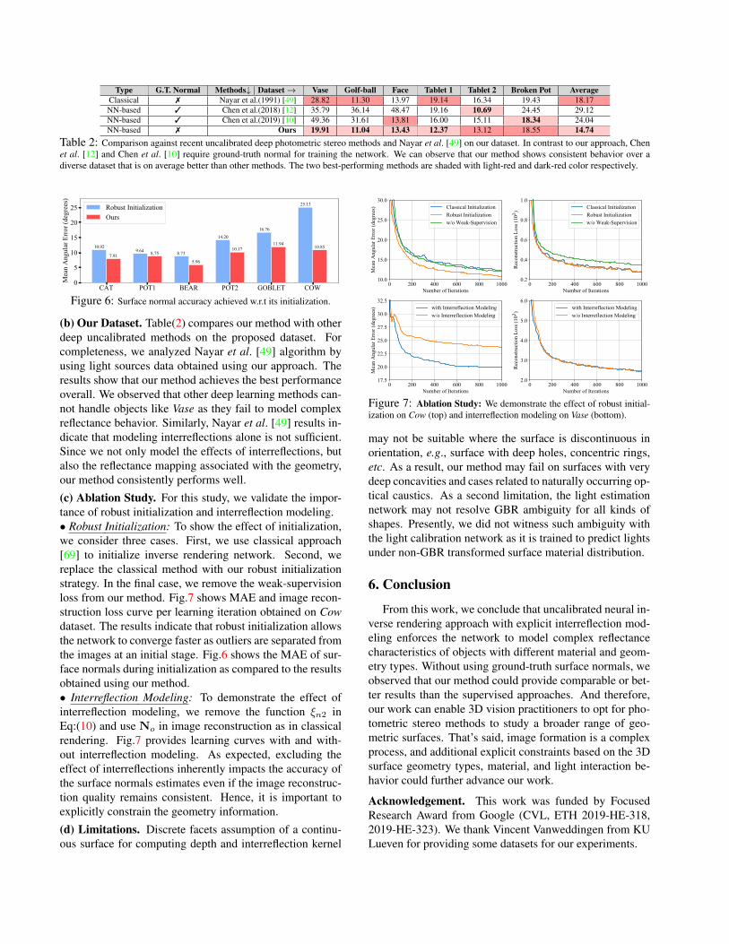
Type G.T. Normal Methods↓ | Dataset→ Vase Golf-ball Face Tablet 1 Tablet 2 Broken Pot AverageClassical 7 Nayar et al.(1991) [49] 28.82 11.30 13.97 19.14 16.34 19.43 18.17NN-based 3 Chen et al.(2018) [12] 35.79 36.14 48.47 19.16 10.69 24.45 29.12NN-based 3 Chen et al.(2019) [10] 49.36 31.61 13.81 16.00 15.11 18.34 24.04NN-based 7 Ours 19.91 11.04 13.43 12.37 13.12 18.55 14.74

Table 2: Comparison against recent uncalibrated deep photometric stereo methods and Nayar et al. [49] on our dataset. In contrast to our approach, Chenet al. [12] and Chen et al. [10] require ground-truth normal for training the network. We can observe that our method shows consistent behavior over adiverse dataset that is on average better than other methods. The two best-performing methods are shaded with light-red and dark-red color respectively.

CAT POT1 BEAR POT2 GOBLET COW0

5

10

15

20

25

Mea

n A

ngul

ar E

rror

(deg

rees

)

10.929.64 8.73

14.2016.76

25.13

7.91 8.75

5.96

10.1711.94

10.85

Robust InitializationOurs

Figure 6: Surface normal accuracy achieved w.r.t its initialization.

(b) Our Dataset. Table(2) compares our method with otherdeep uncalibrated methods on the proposed dataset. Forcompleteness, we analyzed Nayar et al. [49] algorithm byusing light sources data obtained using our approach. Theresults show that our method achieves the best performanceoverall. We observed that other deep learning methods can-not handle objects like Vase as they fail to model complexreflectance behavior. Similarly, Nayar et al. [49] results in-dicate that modeling interreflections alone is not sufficient.Since we not only model the effects of interreflections, butalso the reflectance mapping associated with the geometry,our method consistently performs well.

(c) Ablation Study. For this study, we validate the impor-tance of robust initialization and interreflection modeling.• Robust Initialization: To show the effect of initialization,we consider three cases. First, we use classical approach[69] to initialize inverse rendering network. Second, wereplace the classical method with our robust initializationstrategy. In the final case, we remove the weak-supervisionloss from our method. Fig.7 shows MAE and image recon-struction loss curve per learning iteration obtained on Cowdataset. The results indicate that robust initialization allowsthe network to converge faster as outliers are separated fromthe images at an initial stage. Fig.6 shows the MAE of sur-face normals during initialization as compared to the resultsobtained using our method.• Interreflection Modeling: To demonstrate the effect ofinterreflection modeling, we remove the function ξn2 inEq:(10) and use No in image reconstruction as in classicalrendering. Fig.7 provides learning curves with and with-out interreflection modeling. As expected, excluding theeffect of interreflections inherently impacts the accuracy ofthe surface normals estimates even if the image reconstruc-tion quality remains consistent. Hence, it is important toexplicitly constrain the geometry information.

(d) Limitations. Discrete facets assumption of a continu-ous surface for computing depth and interreflection kernel

Figure 7: Ablation Study: We demonstrate the effect of robust initial-ization on Cow (top) and interreflection modeling on Vase (bottom).

may not be suitable where the surface is discontinuous inorientation, e.g., surface with deep holes, concentric rings,etc. As a result, our method may fail on surfaces with verydeep concavities and cases related to naturally occurring op-tical caustics. As a second limitation, the light estimationnetwork may not resolve GBR ambiguity for all kinds ofshapes. Presently, we did not witness such ambiguity withthe light calibration network as it is trained to predict lightsunder non-GBR transformed surface material distribution.

6. Conclusion

From this work, we conclude that uncalibrated neural in-verse rendering approach with explicit interreflection mod-eling enforces the network to model complex reflectancecharacteristics of objects with different material and geom-etry types. Without using ground-truth surface normals, weobserved that our method could provide comparable or bet-ter results than the supervised approaches. And therefore,our work can enable 3D vision practitioners to opt for pho-tometric stereo methods to study a broader range of geo-metric surfaces. That’s said, image formation is a complexprocess, and additional explicit constraints based on the 3Dsurface geometry types, material, and light interaction be-havior could further advance our work.

Acknowledgement. This work was funded by FocusedResearch Award from Google (CVL, ETH 2019-HE-318,2019-HE-323). We thank Vincent Vanweddingen from KULueven for providing some datasets for our experiments.

References[1] Neil Alldrin, Todd Zickler, and David Kriegman. Photo-

metric stereo with non-parametric and spatially-varying re-flectance. In 2008 IEEE Conference on Computer Vision andPattern Recognition, pages 1–8. IEEE, 2008.

[2] Neil G Alldrin, Satya P Mallick, and David J Kriegman. Re-solving the generalized bas-relief ambiguity by entropy min-imization. In 2007 IEEE conference on computer vision andpattern recognition, pages 1–7. IEEE, 2007.

[3] Doris Antensteiner, Svorad Stolc, and Thomas Pock. Areview of depth and normal fusion algorithms. Sensors,18(2):431, 2018.

[4] Louis-Philippe Asselin, Denis Laurendeau, and Jean-Francois Lalonde. Deep SVBRDF estimation on real mate-rials. In 2020 International Conference on 3D Vision (3DV).IEEE, nov 2020.

[5] Peter N Belhumeur, David J Kriegman, and Alan L Yuille.The bas-relief ambiguity. International journal of computervision, 35(1):33–44, 1999.

[6] Sai Bi, Zexiang Xu, Kalyan Sunkavalli, David Kriegman,and Ravi Ramamoorthi. Deep 3d capture: Geometry and re-flectance from sparse multi-view images. In Proceedings ofthe IEEE/CVF Conference on Computer Vision and PatternRecognition, pages 5960–5969, 2020.

[7] James F Blinn. Models of light reflection for computer syn-thesized pictures. In Proceedings of the 4th annual con-ference on Computer graphics and interactive techniques,pages 192–198, 1977.

[8] Stephen Boyd, Neal Parikh, Eric Chu, Borja Peleato, andJonathan Eckstein. Distributed optimization and statisticallearning via the alternating direction method of multipliers.Foundations and Trends® in Machine Learning, 3(1):1–122,2011.

[9] Manmohan Krishna Chandraker, Fredrik Kahl, and David JKriegman. Reflections on the generalized bas-relief ambi-guity. In 2005 IEEE Computer Society Conference on Com-puter Vision and Pattern Recognition (CVPR’05), volume 1,pages 788–795. IEEE, 2005.

[10] Guanying Chen, Kai Han, Boxin Shi, Yasuyuki Matsushita,and Kwan-Yee K Wong. Self-calibrating deep photometricstereo networks. In Proceedings of the IEEE Conferenceon Computer Vision and Pattern Recognition, pages 8739–8747, 2019.

[11] Guanying Chen, Kai Han, Boxin Shi, Yasuyuki Matsushita,and Kwan-Yee Kenneth Wong. Deep photometric stereofor non-lambertian surfaces. IEEE Transactions on PatternAnalysis and Machine Intelligence, 2020.

[12] Guanying Chen, Kai Han, and Kwan-Yee K Wong. Ps-fcn: Aflexible learning framework for photometric stereo. In Pro-ceedings of the European Conference on Computer Vision(ECCV), pages 3–18, 2018.

[13] Guanying Chen, Michael Waechter, Boxin Shi, Kwan-Yee KWong, and Yasuyuki Matsushita. What is learned in deepuncalibrated photometric stereo? In European Conferenceon Computer Vision, 2020.

[14] Lixiong Chen, Yinqiang Zheng, Boxin Shi, Art Subpa-asa,and Imari Sato. A microfacet-based model for photometric

stereo with general isotropic reflectance. IEEE Transactionson Pattern Analysis and Machine Intelligence, 2019.

[15] Zhang Chen, Anpei Chen, Guli Zhang, Chengyuan Wang, YuJi, Kiriakos N Kutulakos, and Jingyi Yu. A neural renderingframework for free-viewpoint relighting. In Proceedings ofthe IEEE/CVF Conference on Computer Vision and PatternRecognition, pages 5599–5610, 2020.

[16] Hin-Shun Chung and Jiaya Jia. Efficient photometric stereoon glossy surfaces with wide specular lobes. In 2008 IEEEConference on Computer Vision and Pattern Recognition,pages 1–8. IEEE, 2008.

[17] Keenan Crane. Conformal Geometry Processing. PhD thesis,Caltech, June 2013.

[18] Ondrej Drbohlav and M Chaniler. Can two specular pixelscalibrate photometric stereo? In Tenth IEEE InternationalConference on Computer Vision (ICCV’05) Volume 1, vol-ume 2, pages 1850–1857. IEEE, 2005.

[19] Kenji Enomoto, Michael Waechter, Kiriakos N Kutulakos,and Yasuyuki Matsushita. Photometric stereo via discretehypothesis-and-test search. In Proceedings of the IEEE/CVFConference on Computer Vision and Pattern Recognition,pages 2311–2319, 2020.

[20] Yasutaka Furukawa and Jean Ponce. Accurate, dense, androbust multiview stereopsis. IEEE transactions on patternanalysis and machine intelligence, 32(8):1362–1376, 2009.

[21] Athinodoros S Georghiades. Incorporating the torrance andsparrow model of reflectance in uncalibrated photometricstereo. In ICCV, pages 816–823. IEEE, 2003.

[22] Dan B Goldman, Brian Curless, Aaron Hertzmann, andSteven M Seitz. Shape and spatially-varying brdfs from pho-tometric stereo. IEEE Transactions on Pattern Analysis andMachine Intelligence, 32(6):1060–1071, 2009.

[23] Elaine T Hale, Wotao Yin, and Yin Zhang. Fixed-pointcontinuation for l1-minimization: Methodology and conver-gence. SIAM Journal on Optimization, 19(3):1107–1130,2008.

[24] Richard Hartley and Andrew Zisserman. Multiple view ge-ometry in computer vision. Cambridge university press,2003.

[25] Steffen Herbort and Christian Wohler. An introduction toimage-based 3d surface reconstruction and a survey of pho-tometric stereo methods. 3D Research, 2(3):4, 2011.

[26] Tomoaki Higo, Yasuyuki Matsushita, and Katsushi Ikeuchi.Consensus photometric stereo. In 2010 IEEE computer soci-ety conference on computer vision and pattern recognition,pages 1157–1164. IEEE, 2010.

[27] Santo Hiroaki, Michael Waechter, and Yasuyuki Matsushita.Deep near-light photometric stereo for spatially varying re-flectances. In European Conference on Computer Vision,2020.

[28] Satoshi Ikehata. Cnn-ps: Cnn-based photometric stereo forgeneral non-convex surfaces. In Proceedings of the Euro-pean Conference on Computer Vision (ECCV), pages 3–18,2018.

[29] Satoshi Ikehata and Kiyoharu Aizawa. Photometric stereousing constrained bivariate regression for general isotropic

surfaces. In Proceedings of the IEEE Conference on Com-puter Vision and Pattern Recognition, pages 2179–2186,2014.

[30] Satoshi Ikehata, David Wipf, Yasuyuki Matsushita, and Kiy-oharu Aizawa. Robust photometric stereo using sparse re-gression. In 2012 IEEE Conference on Computer Vision andPattern Recognition, pages 318–325. IEEE, 2012.

[31] Satoshi Ikehata, David Wipf, Yasuyuki Matsushita, and Kiy-oharu Aizawa. Photometric stereo using sparse bayesianregression for general diffuse surfaces. IEEE Transactionson Pattern Analysis and Machine Intelligence, 36(9):1816–1831, 2014.

[32] Sergey Ioffe and Christian Szegedy. Batch normalization:Accelerating deep network training by reducing internal co-variate shift. In International conference on machine learn-ing, pages 448–456. PMLR, 2015.

[33] Micah K Johnson and Edward H Adelson. Shape estimationin natural illumination. In CVPR 2011, pages 2553–2560.IEEE, 2011.

[34] Diederik P. Kingma and Jimmy Ba. Adam: A method forstochastic optimization. In Yoshua Bengio and Yann LeCun,editors, 3rd International Conference on Learning Represen-tations, ICLR 2015, San Diego, CA, USA, May 7-9, 2015,Conference Track Proceedings, 2015.

[35] Suryansh Kumar. Jumping manifolds: Geometry awaredense non-rigid structure from motion. In Proceedings of theIEEE Conference on Computer Vision and Pattern Recogni-tion, pages 5346–5355, 2019.

[36] Suryansh Kumar, Yuchao Dai, and Hongdong Li. Monoculardense 3d reconstruction of a complex dynamic scene fromtwo perspective frames. In Proceedings of the IEEE Inter-national Conference on Computer Vision, pages 4649–4657,2017.

[37] Suryansh Kumar, Yuchao Dai, and Hongdong Li. Superpixelsoup: Monocular dense 3d reconstruction of a complex dy-namic scene. IEEE Transactions on Pattern Analysis andMachine Intelligence, 2019.

[38] Junxuan Li, Antonio Robles-Kelly, Shaodi You, and Ya-suyuki Matsushita. Learning to minify photometric stereo.In Proceedings of the IEEE Conference on Computer Visionand Pattern Recognition, pages 7568–7576, 2019.

[39] Min Li, Zhenglong Zhou, Zhe Wu, Boxin Shi, ChangyuDiao, and Ping Tan. Multi-view photometric stereo: A ro-bust solution and benchmark dataset for spatially varyingisotropic materials. IEEE Transactions on Image Process-ing, 29:4159–4173, 2020.

[40] Zhouchen Lin, Minming Chen, and Yi Ma. The augmentedlagrange multiplier method for exact recovery of corruptedlow-rank matrices. arXiv preprint arXiv:1009.5055, 2010.

[41] Fotios Logothetis, Ignas Budvytis, Roberto Mecca, andRoberto Cipolla. A CNN based approach for the near-fieldphotometric stereo problem. In 31st British Machine VisionConference 2020, BMVC 2020, Virtual Event, UK, Septem-ber 7-10, 2020. BMVA Press, 2020.

[42] Fotios Logothetis, Ignas Budvytis, Roberto Mecca, andRoberto Cipolla. Px-net: Simple, efficient pixel-wisetraining of photometric stereo networks. arXiv preprintarXiv:2008.04933, 2020.

[43] Fotios Logothetis, Roberto Mecca, and Roberto Cipolla. Adifferential volumetric approach to multi-view photometricstereo. In Proceedings of the IEEE International Conferenceon Computer Vision, pages 1052–1061, 2019.

[44] Feng Lu, Xiaowu Chen, Imari Sato, and Yoichi Sato. Symps:Brdf symmetry guided photometric stereo for shape and lightsource estimation. IEEE transactions on pattern analysisand machine intelligence, 40(1):221–234, 2017.

[45] Feng Lu, Yasuyuki Matsushita, Imari Sato, Takahiro Okabe,and Yoichi Sato. Uncalibrated photometric stereo for un-known isotropic reflectances. In Proceedings of the IEEEConference on Computer Vision and Pattern Recognition,pages 1490–1497, 2013.

[46] Wojciech Matusik. A data-driven reflectance model. PhDthesis, Massachusetts Institute of Technology, 2003.

[47] Daisuke Miyazaki, Kenji Hara, and Katsushi Ikeuchi. Me-dian photometric stereo as applied to the segonko tumulusand museum objects. International Journal of Computer Vi-sion, 86(2-3):229, 2010.

[48] Yasuhiro Mukaigawa, Yasunori Ishii, and Takeshi Shaku-naga. Analysis of photometric factors based on photometriclinearization. JOSA A, 24(10):3326–3334, 2007.

[49] Shree K Nayar, Katsushi Ikeuchi, and Takeo Kanade. Shapefrom interreflections. International Journal of Computer Vi-sion, 6(3):173–195, 1991.

[50] Tae-Hyun Oh, Hyeongwoo Kim, Yu-Wing Tai, Jean-CharlesBazin, and In So Kweon. Partial sum minimization of sin-gular values in rpca for low-level vision. In Proceedings ofthe IEEE international conference on computer vision, pages145–152, 2013.

[51] Thoma Papadhimitri and Paolo Favaro. A new perspectiveon uncalibrated photometric stereo. In Proceedings of theIEEE Conference on Computer Vision and Pattern Recogni-tion, pages 1474–1481, 2013.

[52] Thoma Papadhimitri and Paolo Favaro. A closed-form, con-sistent and robust solution to uncalibrated photometric stereovia local diffuse reflectance maxima. International journalof computer vision, 107(2):139–154, 2014.

[53] Jaesik Park, Sudipta N Sinha, Yasuyuki Matsushita, Yu-Wing Tai, and In So Kweon. Multiview photometric stereousing planar mesh parameterization. In Proceedings of theIEEE International Conference on Computer Vision, pages1161–1168, 2013.

[54] Adam Paszke, Sam Gross, Soumith Chintala, GregoryChanan, Edward Yang, Zachary DeVito, Zeming Lin, Al-ban Desmaison, Luca Antiga, and Adam Lerer. Automaticdifferentiation in pytorch. 2017.

[55] Yvain Queau, Tao Wu, Francois Lauze, Jean-Denis Durou,and Daniel Cremers. A non-convex variational approach tophotometric stereo under inaccurate lighting. In Proceed-ings of the IEEE Conference on Computer Vision and PatternRecognition, pages 99–108, 2017.

[56] Hiroaki Santo, Masaki Samejima, Yusuke Sugano, BoxinShi, and Yasuyuki Matsushita. Deep photometric stereo net-work. In Proceedings of the IEEE International Conferenceon Computer Vision Workshops, pages 501–509, 2017.

[57] Johannes L Schonberger and Jan-Michael Frahm. Structure-from-motion revisited. In Proceedings of the IEEE Con-ference on Computer Vision and Pattern Recognition, pages4104–4113, 2016.

[58] Soumyadip Sengupta, Angjoo Kanazawa, Carlos D Castillo,and David W Jacobs. Sfsnet: Learning shape, reflectanceand illuminance of facesin the wild’. In Proceedings of theIEEE Conference on Computer Vision and Pattern Recogni-tion, pages 6296–6305, 2018.

[59] Soumyadip Sengupta, Hao Zhou, Walter Forkel, RonenBasri, Tom Goldstein, and David Jacobs. Solving uncali-brated photometric stereo using fewer images by jointly op-timizing low-rank matrix completion and integrability. Jour-nal of Mathematical Imaging and Vision, 60(4):563–575,2018.

[60] Boxin Shi, Yasuyuki Matsushita, Yichen Wei, Chao Xu, andPing Tan. Self-calibrating photometric stereo. In 2010 IEEEComputer Society Conference on Computer Vision and Pat-tern Recognition, pages 1118–1125. IEEE, 2010.

[61] Boxin Shi, Ping Tan, Yasuyuki Matsushita, and KatsushiIkeuchi. Bi-polynomial modeling of low-frequency re-flectances. IEEE transactions on pattern analysis and ma-chine intelligence, 36(6):1078–1091, 2013.

[62] Boxin Shi, Zhe Wu, Zhipeng Mo, Dinglong Duan, Sai-KitYeung, and Ping Tan. A benchmark dataset and evaluationfor non-lambertian and uncalibrated photometric stereo. InProceedings of the IEEE Conference on Computer Visionand Pattern Recognition, pages 3707–3716, 2016.

[63] Richard Szeliski. Computer vision: algorithms and applica-tions. Springer Science & Business Media, 2010.

[64] Ping Tan, Satya P Mallick, Long Quan, David J Kriegman,and Todd Zickler. Isotropy, reciprocity and the generalizedbas-relief ambiguity. In 2007 IEEE Conference on ComputerVision and Pattern Recognition, pages 1–8. IEEE, 2007.

[65] Tatsunori Taniai and Takanori Maehara. Neural inverse ren-dering for general reflectance photometric stereo. In Inter-national Conference on Machine Learning (ICML), pages4857–4866, 2018.

[66] Xueying Wang, Yudong Guo, Bailin Deng, and JuyongZhang. Lightweight photometric stereo for facial detailsrecovery. In Proceedings of the IEEE/CVF Conference onComputer Vision and Pattern Recognition, pages 740–749,2020.

[67] Xi Wang, Zhenxiong Jian, and Mingjun Ren. Non-lambertian photometric stereo network based on inverse re-flectance model with collocated light. IEEE Transactions onImage Processing, 29:6032–6042, 2020.

[68] Olivia Wiles and Andrew Zisserman. SilNet : Single- andmulti-view reconstruction by learning from silhouettes. InProcedings of the British Machine Vision Conference 2017.British Machine Vision Association, 2017.

[69] Robert J Woodham. Photometric method for determiningsurface orientation from multiple images. Optical engineer-ing, 19(1):191139, 1980.

[70] Changchang Wu, Sameer Agarwal, Brian Curless, andSteven M Seitz. Schematic surface reconstruction. In 2012IEEE Conference on Computer Vision and Pattern Recogni-tion, pages 1498–1505. IEEE, 2012.

[71] Lun Wu, Arvind Ganesh, Boxin Shi, Yasuyuki Matsushita,Yongtian Wang, and Yi Ma. Robust photometric stereo vialow-rank matrix completion and recovery. In Asian Confer-ence on Computer Vision, pages 703–717. Springer, 2010.

[72] Tai-Pang Wu and Chi-Keung Tang. Photometric stereo viaexpectation maximization. IEEE transactions on patternanalysis and machine intelligence, 32(3):546–560, 2009.

[73] Zhe Wu and Ping Tan. Calibrating photometric stereo byholistic reflectance symmetry analysis. In Proceedings of theIEEE Conference on Computer Vision and Pattern Recogni-tion, pages 1498–1505, 2013.

[74] Bing Xu, Naiyan Wang, Tianqi Chen, and Mu Li. Empiricalevaluation of rectified activations in convolutional network.arXiv preprint arXiv:1505.00853, 2015.

[75] Zhuokun Yao, Kun Li, Ying Fu, Haofeng Hu, and BoxinShi. Gps-net: Graph-based photometric stereo network. Ad-vances in Neural Information Processing Systems, 33, 2020.

[76] Enliang Zheng and Changchang Wu. Structure from motionusing structure-less resection. In Proceedings of the IEEEInternational Conference on Computer Vision, pages 2075–2083, 2015.

[77] Qian Zheng, Yiming Jia, Boxin Shi, Xudong Jiang, Ling-Yu Duan, and Alex C Kot. Spline-net: Sparse photometricstereo through lighting interpolation and normal estimationnetworks. In Proceedings of the IEEE International Confer-ence on Computer Vision, pages 8549–8558, 2019.

[Supplementary Material] Uncalibrated Neural Inverse Rendering for Photomet-ric Stereo of General Surfaces

Abstract

In our supplementary material, we first present a fewcase studies to analyze our method’s effectiveness. Next, wegive a detailed description of our coding implementation fortraining and testing the neural network outlined in the mainpaper. Formally, this report includes the coding platformdetails —both hardware and software, with train and testtime observed across different datasets. Further, mathemat-ical derivations of our robust initialization and specular-reflectance map formulations are supplied. Finally, we an-alyze the light estimation performance and discuss the pos-sible future extensions of our method. Besides, our supple-mentary material includes a short video clip that illustratesthe image acquisition setup and visual results.

A. Case StudyThis section provides the observation on the case study

that we conducted for our proposed method. It is done toanalyze the behavior of our method under different possiblevariations in our experimental setup. Such a study can helpus understand the behavior, pros, and cons of our approach.Case Study 1: What if we use ground-truth light as inputto inverse rendering network instead of relying on light es-timation network?

This case study investigates the reliability of our method.To conduct this experiment, we supplied ground-truth lightsource directions and intensities as input to the inverse ren-dering network and robust initialization. The goal is tostudy the expected deviation in the accuracy of surface nor-mals when ground-truth light sources information is used,compared to the light calibration network. Table (3) com-pares our method’s performance with recent deep calibratedphotometric stereo methods on our proposed dataset. Theresults show that our inverse rendering method achievesthe best performance in the calibrated setting, although itdoes not use a training dataset like other deep-learning-based methods. Additionally, we observed that the CNNPSmodel proposed by Ikehata [28] which performs per-pixelestimation using observation maps, may not provide accu-rate surface normals for interreflecting surfaces such as theVase and the Broken Pot. Hence, we conclude that extract-ing information by utilizing the surface geometry is crucialfor solving photometric stereo since all surface points affecteach other.

Moreover, in Table (3), we show the comparison of ourmethod’s performance under calibrated and uncalibratedsettings. Our method achieves 12.68 MAE on average, us-ing ground-truth light as input. At the same time, it reaches

90°

0°Rose Dataset Ground-truth Normal Estimated Normal Error Map

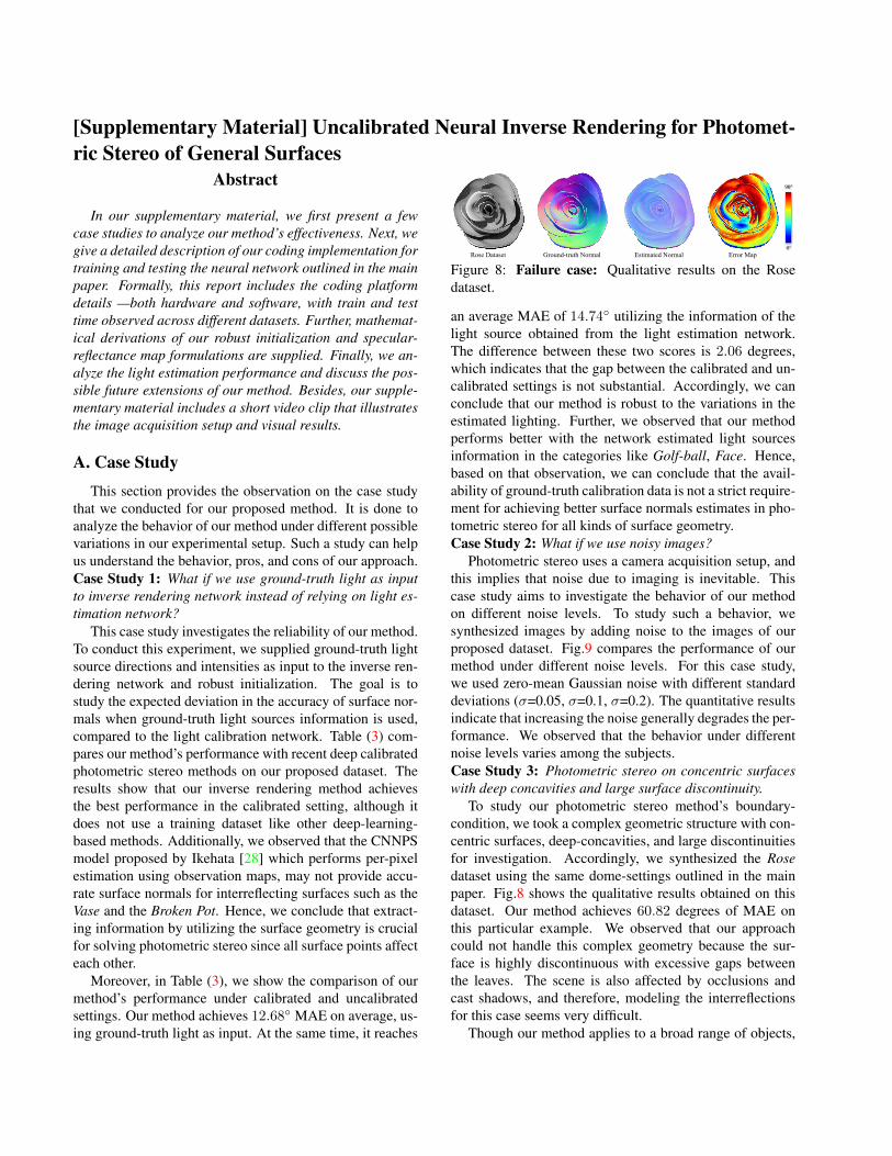
Figure 8: Failure case: Qualitative results on the Rosedataset.

an average MAE of 14.74 utilizing the information of thelight source obtained from the light estimation network.The difference between these two scores is 2.06 degrees,which indicates that the gap between the calibrated and un-calibrated settings is not substantial. Accordingly, we canconclude that our method is robust to the variations in theestimated lighting. Further, we observed that our methodperforms better with the network estimated light sourcesinformation in the categories like Golf-ball, Face. Hence,based on that observation, we can conclude that the avail-ability of ground-truth calibration data is not a strict require-ment for achieving better surface normals estimates in pho-tometric stereo for all kinds of surface geometry.Case Study 2: What if we use noisy images?

Photometric stereo uses a camera acquisition setup, andthis implies that noise due to imaging is inevitable. Thiscase study aims to investigate the behavior of our methodon different noise levels. To study such a behavior, wesynthesized images by adding noise to the images of ourproposed dataset. Fig.9 compares the performance of ourmethod under different noise levels. For this case study,we used zero-mean Gaussian noise with different standarddeviations (σ=0.05, σ=0.1, σ=0.2). The quantitative resultsindicate that increasing the noise generally degrades the per-formance. We observed that the behavior under differentnoise levels varies among the subjects.Case Study 3: Photometric stereo on concentric surfaceswith deep concavities and large surface discontinuity.

To study our photometric stereo method’s boundary-condition, we took a complex geometric structure with con-centric surfaces, deep-concavities, and large discontinuitiesfor investigation. Accordingly, we synthesized the Rosedataset using the same dome-settings outlined in the mainpaper. Fig.8 shows the qualitative results obtained on thisdataset. Our method achieves 60.82 degrees of MAE onthis particular example. We observed that our approachcould not handle this complex geometry because the sur-face is highly discontinuous with excessive gaps betweenthe leaves. The scene is also affected by occlusions andcast shadows, and therefore, modeling the interreflectionsfor this case seems very difficult.

Though our method applies to a broad range of objects,

Type G.T. Normal Methods↓ | Dataset→ Vase Golf-ball Face Tablet 1 Tablet 2 Broken Pot Average PerformanceNN-based 3 Ikehata (2018)[28] 34.00 14.96 16.61 16.64 12.32 18.31 18.81NN-based 3 Chen et al.(PS-FCN)(2018)[12] 27.11 15.99 16.17 10.23 5.79 8.68 14.00NN-based 7 Ours (Ground-truth light/ calibrated) 16.40 14.23 14.24 10.77 4.49 15.92 12.68NN-based 7 Ours (Estimated light/ uncalibrated) 19.91 11.04 13.43 12.37 13.12 18.55 14.74

Diff. in MAE (Ours(Est)-Ours(GT)) +3.51 -3.19 -0.81 +1.60 +8.63 +2.63 +2.06

Table 3: Comparison of recent deep calibrated photometric stereo methods Ikehata [28] and Chen et al. [12] (PS-FCN) against our method underuncalibrated and calibrated setting. For testing our method under the calibrated setting, we evaluate the performances assuming that ground-truth lightsource directions and intensities are available. Note that Chen et al. [12] and Ikehata [28] additionally uses ground-truth surface normals for training, incontrast to our method. The last row shows the difference between our method results when used under uncalibrated and calibrated setting respectively. Wecan see that the average difference in MAE between the two settings of our method is not significant.

our interreflection modeling is inspired by Nayar et al. [49]formulation, which may not hold for all kinds of surfaces.The interreflection modeling computes depth from the nor-mal map under the continuous surface assumption, whichfails in this case study. Furthermore, it models continuoussurfaces with discrete facets. Due to such limitations, ourmethod may not be suitable for concentric surfaces withdeep concavities and large discontinuities. In such cases,the interreflection effect is very complicated, and our ap-proach may disappoint to model such complex light phe-nomena.

B. Coding DetailsThis section provides a detailed description of our source

code implementation. We start by introducing the light es-timation network’s training phase. Then we focus on thetesting phase, where the inverse rendering network is op-timized to estimate the surface normals, depth, and BRDFvalues. Finally, we present details on training and testingrun-times.

B.1. Training Details

As our inverse rendering network optimizes its learnableparameters at the test time, we apply a training stage only tothe light estimation network. For training the network, weused Blobby and Sculpture datasets that are introduced byChen et al. [12]. This dataset is created by using 3D geome-tries of Blobby [33], and Sculpture [68] shape datasets andcombining them with different material BRDFs taken fromMERL dataset [46]. In total, the complete dataset contains85212 subjects. For each subject, there exist 64 renderingswith different light source directions. The intensity of thelight sources is kept constant during the whole data genera-tion process. To simulate different intensities during train-ing, image intensity values are randomly generated in therange of [0.2, 2], and these intensity values are used to scalethe image data linearly. In each training iteration, the inputdata is perturbed in the range of [−0.025, 0.025] for aug-mentation.

The light estimation network is a multiple-inputmultiple-output (MIMO) system which requires images ofthe same object captured under different illumination con-ditions (see Fig.10). The core idea is that all input images

Noise Std (σ) Vase Golf-ball Face Tablet1 Tablet2 Broken Pot Average

0.0 19.91 11.01 13.43 12.37 13.12 18.55 14.73

0.05 21.96 11.54 12.94 17.25 11.22 17.22 15.36

0.1 25.01 11.83 15.12 18.80 11.55 19.06 16.90

0.2 24.41 14.25 19.62 21.27 10.07 18.16 17.96

Mea

n A

ngul

ar E

rror

0

5.2

10.4

15.6

20.8

26

DatasetVase Golf-ball Face Tablet1 Tablet2 Broken Pot Average

0.0 0.05 0.1 0.2σ σ σ σ

1

Figure 9: The performance of our method against different noise lev-els. We used zero-mean Gaussian noise (µ = 0) with different standarddeviations (σ). We observed that increasing the noise level generally de-grades the performance. Still, the behavior under different noise levelsvaries among the subjects as the performance depends on the signal-to-noise ratio of the images.

have the same surface, and having more images helps thenetwork extract better global features. During training, weuse 32 images of the same object for global feature extrac-tion. Note that all of the images are used for feature extrac-tion at test time to achieve the best performance from thenetwork.

B.2. Testing Details

Given a set of test images X and object mask O, wefirst use the light estimation network to have light source di-rections and intensities. However, the light estimation net-work operates on 128 × 128 images because it uses fullyconnected layers for classification, and these layers processonly fixed-length vectors. Consequently, we scale the inputimages into the resolution of 128×128 before feeding themto the network. We apply this pre-processing step only forthe light estimation network and use the original image sizefor all other operations during testing.

Once we obtain the light source directions and intensi-ties, we apply the robust initialization algorithm to get aninitial surface normal matrix Ninit. It also provides analbedo map that is transformed into P ∈ Rm×m which is re-quired for interreflection modeling. Details about the robustinitialization method are explained and derived in §C.1.

After the robust initialization process, we start the op-timization of our inverse rendering framework. First, we

128

128

643128

128 128128 256

256

3 × 3 Conv

(Stride: 2)

LReLU

3 × 3 Conv

(Stride: 2)

LReLU

3 × 3 Conv

(Stride: 2)

LReLU

3 × 3 Conv

(Stride: 1)

LReLU

3 × 3 Conv

(Stride: 2)

LReLU

3 × 3 Conv

(Stride: 1)

LReLU

3 × 3 Conv

(Stride: 2)

LReLU

64

128

128

643128

128 128128 256

256

Maxpooling

3 × 3 Conv

(Stride: 1)

LReLU

3 × 3 Conv

(Stride: 2)

LReLU

3 × 3 Conv

(Stride: 2)

LReLUFully Connected

Layer

Fully Connected

Layer

256256

64

256

20

72

512

64

256256

64

256

20

72

512

256

e1

l1

e𝑛

l𝑛

.

.

.

X1

X𝑛

.

.

.

256

256

3 × 3 Conv

(Stride: 2)

LReLU

Figure 10: Architecture of the light estimation network. The network first extracts features from the input images separately using featureextraction layers (purple). Then, the extracted image-specific features (light-green) are fused with max-pooling operation to obtain a global representationof the entire scene (dark-green). Finally, all image-specific and global features are used in classifier network where convolution (brown) and fully-connected(blue) layers are used to predict light intensity values (ei’s) and direction vectors (li’s).

initialize all the network parameters (Θf , Θn1, Θsp, Θlg

Θri) which correspond to the weights of the convolutionoperations. In this step, we initialize the weights randomlyby sampling from a Gaussian distribution with zero meanand 0.02 variance. We perform 1000 iterations in total us-ing Adam optimizer [34] with an initial learning rate of8 × 10−4. The learning rate is reduced by a factor of 10after 900 iterations for fine-tuning. We observed that settingthese hyperparameters may result in convergence problemsin our dataset. For this reason, we set the initial learningrate of the estimation branch (ξf and ξn1) to 8×10−5 whileexperimenting on our dataset. We also inject Gaussian noisewith zero mean and 0.1 variance to the images before feed-ing them to fsp for image reconstruction. We observed thatthis prohibits the network from generating degenerate solu-tions. At every 100 iterations, we update the depth and theinterreflection kernel matrix entries using the normal esti-mation No.(a) Depth: To compute the depth from normals, we use agradient-based method with surface orientation constraint[3]. Given the surface normals, we first compute a gradientfield G ∈ Rh×w×2 where h and w are the spatial dimen-sions. The idea is that the gradient field computed fromsurface normal map and the estimated depth D ∈ Rh×wshould be consistent, i.e., ∇D ≈ G. That corresponds toan overdetermined system of linear equations and is solvedby minimizing the following objective function i.e., Eq:(19)using the least-squares approach

min.D‖∇D− G‖2 (19)

(b) Interreflection Modeling: To consider the effect of in-terreflection during the image reconstruction process, wedefine the function ξn2 which uses the estimated normalNo ∈ R3×m, albedo matrix P ∈ Rm×m and the inter-

reflection kernel K ∈ Rm×m. Given all these components,Nayar et al. [49] relates the observed radiance (X) and theradiance due to primary light source (Xs) as follows:

X = (I−PK)−1Xs (20)

Assuming the surface shows Lambertian reflectanceproperty, we model the radiance in terms of facet matricesas follows:

X = FnyL, Xs = FL, ⇒ Fny = (I−PK)−1F(21)

Here Fny ∈ Rm×3 and F ∈ Rm×3 are the facet matri-ces which contain surface normals Nny and No scaled withlocal reflectance value. We use Eq:(21) to obtain Fny andnormalize each row to unit vector to obtain Nny .

The computation of the interreflection kernel K has thecomplexity of O(n2) where n is the number of facets.Therefore, treating each pixel as a facet limits the applica-tion of our method. To approximate the effect of interreflec-tions, we downsample the normal maps with the factor of 4and calculated the kernel values accordingly. After the nor-mal is updated, we scale it to the original size managing theimage details appropriately.

B.3. Timing Details

Our framework is implemented in Python using PyTorchversion 1.1.0. Table (4) provides the light estimation net-work’s training time and the inference time of neural inverserendering network on two datasets separately.

C. Mathematical DerivationsHere, we supply the mathematical derivation pertaining

to the initialization of the surface normals to the inverse ren-

CAT POT2 GOBLET READING COWBUDDHABALL POT1 BEAR HARVEST

90°

0°

(a) DiLiGenT Dataset

(b) Ground-Truth Normal

(c) Our Estimated Normal

(d) Error Map

Figure 11: We present visual results of our method on all of the DiLiGenT categories. The bottom row demonstrates theangular error maps obtained form our estimations and ground-truth normals.

dering network. For completion, we also supplied the well-known deviation of reflection vector §C.2.

C.1. Robust Initialization

Our surface normals initialization procedure aims at re-covering the low rank matrix Z ∈ Rm×n from the imagematrix X ∈ Rm×n such that X = Z+E where E ∈ Rm×nis the matrix of outliers. Here, we assume that the low-rank matrix follows the classical photometric stereo model(Z = NTL) and the outlier matrix E is sparse in its distri-bution. Since it is known by definition that Z spans a rank-3 space, it can be formulated as a standard RPCA problem[71]. However, we know that RPCA formulation performsthe nuclear norm minimization of Z matrix which not onlyminimizes the rank but also the variance of Z within the tar-get rank. Now, for the photometric stereo model, it is easyto infer that N lies in a rank 3 space. As the true rank forZ is known from its mathematical construction, we do notwant to minimize the subspace variance within the targetrange. Nevertheless, this strict constraint is difficult to meetdue to the complex imaging model, and therefore, we en-courage to preserve the variance of information within thetarget range while minimizing the other singular values out-side the target rank (K). So, we minimize the partial sumof the singular values which are outside the target rank withthe following optimization as follows:

minimizeZ,E

‖Z‖r=K + λ‖E‖1, subject to: X = Z + E

(22)

GPU TimeTraining of Light Estimation Network Titan X Pascal (12GB) ≈ 22 hours

Inference on DiLiGenT GeForce GTX TITAN X (12GB) 53.41± 41.57 min per subjectInference on our Dataset GeForce GTX TITAN X (12GB) 29.08± 15.99 min per subject

Table 4: Measured training and testing time with respect to the utilizedhardware. For our dataset, we have 100 to 260 images per subject andthe DiLiGenT dataset has 96 images per subject. Note: Deep photometricstereo method processes a set of images rather than one image for estimat-ing normals.

The Augmented Lagrangian function of Eq:(22) can bewritten as follows:

L(Z,E,Y) = ‖Z‖r=K + λ‖E‖1 +µ

2‖X− Z−E‖2F+

< Y,X− Z−E >(23)

Here, µ is a positive scalar and Y ∈ Rm×n is the esti-mate of the Lagrange multiplier. As minimizing this func-tion is challenging, we solve it by utilizing the alternatingdirection method of multipliers (ADMM)[8, 50, 40]. Ac-cordingly, the optimization problem in Eq:(23) can be di-vided into sub-problems, where Z, E and Y are updatedalternatively while keeping the other variables fixed.1. Solution to Z:

Z∗ = argminZ‖Z‖r=K +

µk2‖Z− (X−Ek + µ−1

k Yk)‖2F(24)

The solution to Eq:(24) sub-problem at kth itera-tion is given by Zk = PK,µ−1

k[X − Ek + µ−1

k Yk]

where, PK,τ [M] = UM(ΣM1 + Sτ [ΣM2 ])VTM is the

partial singular value thresholding operator [50] andSτ [x] = sign(x) max(|x| − τ, 0) is the soft-thresholding

operator [23]. Here, UM,VM are the singular vec-tor of matrix M and ΣM1 = diag(σ1, σ2, ...σK , 0, 0),ΣM2 = diag(0, 0, .., σK+1, .., σN ).

2. Solution to E:

E∗ = argminE

λ‖E‖1 +µk2‖E− (X− Zk+1 + µ−1

k Yk)‖2F(25)

The solution to Eq:(25) sub-problem at kth iteration isgiven by Ek = Sλµ−1

k[X − Zk+1 + µ−1

k Yk] where,Sτ [x] = sign(x) max(|x| − τ, 0) is a soft-thresholdingoperator [23]. For proof of convergence and theoreticalanalysis of partial singular value thresholding operatorkindly refer to Oh et al. [50] work. We solve for Z, E usingADMM until convergence for K = 3 and use the obtainedsurface normals for initializing the loss function of inverserendering network.

3. Solution to Y: The variable Y is updated as follows overthe iteration:

Yk+1 = Yk + µk(X− Zk+1 −Ek+1) (26)

For more details on the implementation kindly refer to Ohet al. [50] method.

C.2. Derivation of Specular-Reflection Equation 11in the Main Paper

For completion, we derive Equation 11 of the main pa-per that is used to compute the specular-reflection mapRi ∈ Rh×w×1 for each image. To compute it, we first com-pute rxi for each point x that is the direction vector withthe highest specular component using the following well-known relation; assuming li, and no as unit length vectors:

rxi + li = 2cos(θ).no(x); no(x)T li = cos(θ)

rxi = 2(no(x)T li)no(x

)− li

(27)

Here, rxi is also a unit length vector (see Fig.12). Thecomponent of specular reflection in the view-direction v =(0, 0, 1)T of the point x due to ith light is computed as:

rxi = vT(

2(no(x)T li)no(x

)− li

)(28)

The above relation show that the specular highlights arestrongest if the normal no(x) is closest to rxi. Performingthis operation for each point gives us the specular-reflectionmap Ri.

D. Statistical Analysis of Estimated LightSource Directions

We aim to investigate the source directions’ behaviorpredicted by the light estimation network (Fig.10). For that

li

no(x)

rxi v

x

𝜃𝜃

Figure 12: Illustration of surface reflectance. When lightray li hits a surface element, the specular component alongthe view-direction of the point x due to ith source is givenby rxi. This presentation of 3D geometry is inspired byKeenan work [17].

purpose, we use a well-known setup used for light calibra-tion, i.e., a calibration sphere. Our renderings from the cal-ibration sphere (see Fig.13(a)) has specular highlights andattached shadows, which provide useful cues for the lightestimation network. Figures 13(b)-13(d) illustrate the x, yand z components of the estimated light source directionand ground-truth with respect to the images. We measuredthe MAE between these vectors as 6.31 degrees. We alsoobserved that the x and y components match well with theground-truth values. On the other hand, we observed fluctu-ations on the z component where the values slightly deviatefrom the ground-truth in a specific pattern. One possible ex-planation for this observation is that the network has a biassuch that its behavior changes in the different regions of thelighting space. Since we generated the data by moving thelight source on a circular pattern around z-axis, Fig. 13(d)also follows a similar pattern with the same frequency withx and y components’ curves.

E. More Qualitative Results Comparison onour Dataset

Here, we present qualitative results on all of the cate-gories of our proposed dataset. Figure 14 to Figure 19 com-pares the output normal maps of our method with otherbaselines. Note that our implementation of Nayar et al.[49] uses Woodham’s classical photometric stereo [69] tocalculate the pseudo surface and updates the normals withthe interreflection modeling for 15 iterations. Even thoughthe Nayar et al. [49] interreflection algorithm is not theo-retically guaranteed to converge for all surfaces, it gives astable response on our dataset. We initialized Nayar’s algo-rithm using the same predicted light sources of our methodfor a fair comparison.

The results show that our method achieves the best re-sults overall, both qualitatively and quantitatively. We ob-served that other deep learning networks [12, 10] may fail toremove the surface ambiguity in challenging subjects. This

(a) Calibration Sphere

0 20 40 60 80 100Images

1.0

0.5

0.0

0.5

1.0

x C

ompo

nent

EstimatedGround-truth

(b) x Component

0 20 40 60 80 100Images

1.0

0.5

0.0

0.5

1.0

y C

ompo

nent

EstimatedGround-truth

(c) y Component

0 20 40 60 80 100Images

0.0

0.2

0.4

0.6

0.8

1.0

z C

ompo

nent

EstimatedGround-truth

(d) z Component

Figure 13: Light source directions obtained from the calibration sphere (a) using the light estimation network. We demonstrate the x,y and z componentsof the light direction vectors (b-d). The mean angular error between the ground-truth and estimated light directions is 6.31 degrees.

Ball Cat Pot1 Bear Pot2 Buddha Goblet Reading985 2808 3601 2585 2193 2787 1636 1723Cow Harvest Vase Golf-ball Face Tablet 1 Tablet 2 Broken Pot1651 3582 1280 468 435 1610 437 1046

Table 5: Number of facets per subject used for our experiments.

is because these networks require supervised training withground-truth normals, and their performance depends on thecontent of the training dataset. On the other hand, the resultsshow that Nayar et al. [49] performs much better on chal-lenging concave shapes. However, it cannot model spec-ularities and cast shadows. On the other hand, our methodcan model these non-Lambertian effects with the reflectancemapping, and therefore, it performs better than Nayar et al.in all the tested categories.

Lastly, we provide the reflectance map obtained usingour method on the proposed dataset. Figure 20 and Figure21 show the reflectance map obtained using our method onthe synthetic and real sequence respectively.

F. Some General Comments

Q1: Influence of complex texture on the light estima-tion. Indeed, surface texture is can be important for lightestimation. However, the present benchmark datasets i.e.,DiLiGenT is composed of textureless subjects, and there-fore, our focus was to perform surface reconstruction ontextureless objects.

Q2: Nayar interreflection model vs. Monte Carlo:Monte Carlo method can provide more photo-realistic ren-derings. However, such an approach is again expensive, re-quires analytic BRDF models, and a sophisticated samplingstrategy for computation, which can make the pipeline bet-ter, but more involved. So, we favored Nayar’s method andused reflectance maps to handle non-Lambertian effects.Q3: Number of parameters for the normal estimation net-work and interreflection kernel computation: The inverserendering network has ≈3.7 million parameters (12.3 MB).The interreflection kernel is generally sparse, and efficientsoftware are available to handle large-sized sparse matrices.Table (5) provides the number of facets used for our exper-iments to calculate the interreflection kernel.

Nayar et al. (1991) Chen et al. (2018) Chen et al. (2019) OursGround-truth/Input Image

MAE = 28.82° MAE = 35.79° MAE = 49.36° MAE = 19.91°

90°

0°

Figure 14: Qualitative comparison on the Vase scene. Here, it is obviousthat previous deep learning based methods fail to handle the concavity ofthe subject. In contrast, our method works reasonably well showing thecompetence of our modeling procedure.

MAE = 31.61°

Nayar et al. (1991) Chen et al. (2018) Chen et al. (2019) OursGround-truth/Input Image

MAE = 11.30° MAE = 36.14° MAE = 11.04°

90°

0°

Figure 15: Qualitative comparison on the Golf-ball scene. Althoughdeep learning based methods perform well smooth objects, they cannothandle fine structures and indentations.

G. Other Possible Future Extension

Our proposed method enables the application of photo-metric stereo on a broader range of objects. Yet, we thinkthat there are possible future directions to extend it. Firstly,our method is generally a two-stage framework that uti-lizes a light estimation network and inverse rendering net-work in separate phases during inference. As an exten-sion of our work, we aim to combine those stages in anend-to-end framework where light, surface normals, and re-flectance values are estimated simultaneously. Secondly,our method uses a physical rendering equation for imagereconstruction that is not sufficient for modeling all phys-ical interactions between the object and the light. We be-lieve that an improved rendering equation with additionalphysical constraints will allow better normal estimates. Inaddition to that, our method utilizes a specular-reflectance

Nayar et al. (1991) Chen et al. (2018) Chen et al. (2019) OursGround-truth/Input Image

MAE = 13.97° MAE = 48.47° MAE = 13.81° MAE = 13.43°

90°

0°

Figure 16: Qualitative comparison on the Face scene. Although Nayaret al. [49] models interreflections, it cannot handle cast shadows. There-fore, it performs poorly on regions surrounding the eyes and the nose wherecast shadows are effective. Here, we also observe that Chen et al. [12] can-not estimate accurately for higher slant angles.

Nayar et al. (1991) Chen et al. (2018) Chen et al. (2019) OursGround-truth/Input Image

MAE = 19.14° MAE = 19.16° MAE = 16.00° MAE = 12.37°

90°

0°

Figure 17: Qualitative comparison on the Tablet1 scene. This subjecthas a complicated geometry involving cuneiform and reliefs. Apart fromthese fine structures, the object can be treated as a composite surface whichhas a large concavity in the middle part.

Nayar et al. (1991) Chen et al. (2018) Chen et al. (2019) OursGround-truth/Input Image

MAE = 16.34° MAE = 10.69° MAE = 15.11° MAE = 13.12°

90°

0°

Figure 18: Qualitative comparison on the Tablet2 scene. Similar toTablet1, this subject also contains reliefs and cuneiform scripts. Since theoverall geometry is approximately flat, all methods perform comparableon this category.

Nayar et al. (1991) Chen et al. (2018) Chen et al. (2019) OursGround-truth/Input Image

MAE = 19.43° MAE = 24.45° MAE = 18.34° MAE = 18.55°

90°

0°

Figure 19: Qualitative comparison on the Broken Pot scene.

map inspired by the Phong reflectance model. Using othersophisticated variants of specular-reflectance map such asthe Blinn-Phong reflection model [7] may further advanceour approach. Finally, we observed that our method is very

Ref

lect

ance

sIm

ages

Ref

lect

ance

sIm

ages

Ref

lect

ance

sIm

ages

(a) VASE

(b) GOLF-BALL

(c) FACE

Figure 20: Reflectance maps obtained with our method from Vase,Golf-ball and Face categories.

Ref

lect

ance

sIm

ages

Ref

lect

ance

sIm

ages

Ref

lect

ance

sIm

ages

(a) TABLET1

(b) TABLET2

(c) BROKEN POT

Figure 21: Reflectance maps obtained with our method from Tablet1,Tablet2 and Broken Pot categories.

convenient for practical usage as it doesn’t require ground-truth normals for supervised training. However, it could bepossible to improve performance by utilizing training datain a similar framework.