Embed Size (px)
Citation preview

Surveying
Prof. Bharat Lohani
Indian Institute of Technology, Kanpur
Module - 5
Lecture - 3
Theodolites and Total Stations
(Refer Slide Time: 00:31)
Welcome to another lecture on basic surveying. This is module number five and this
module is on theodolites and total stations. Today, we will do lecture number three of
this module.

(Refer Slide Time: 00:33)
Now, what we have done so far? As far as this module is concerned on theodolite and
total stations, we have seen the instrument, the theodolite, why we need to use it and in
particular, in our last lecture we discussed about the telescope, which is used in the
theodolite. And then, from definitions like the line of sight, line of collimation and some
more definitions, which are related to the theodolite. We also saw what is face left
observation, what is face right observation. Then, if you are going to a field and we want
to measure an angle, we saw the procedure last time.
So, there are some steps, which we need to do at every station. These steps are called
temporary adjustments. What we do? We take the theodolite along with the tripod to that
particular point or we can say, survey station. Then, we need to do couple of things.
Number one is centering. We put our tripod over that point, approximately center it;
leveling, we level the tripod height approximately. Then, having done this, put the tripod
or we put the theodolite on top of the tripod and after that we will start doing the
centering of the theodolite, leveling of the theodolite and as well as we do the focusing.
So, having achieved proper centering and leveling, the focusing means, we sight to the
object and we need to focus that. In order to focus the object we need to first focus the
eye piece, so that we can see the cross wires very distinctly. Then, the image through the
objective lens is focused on the plane of the cross wire.

Now, here the term, which is called parallax. Parallax means, if this is the plane of the
cross wire, the image, which is being formed is not at this plane, but rather here. Well,
you may find this is clearly seen in the images, distinctly seen focus image as far your
eyes are concerned. But is there any parallax between them? Yeah, there is the parallax
between them because if you move your eyes here and there slightly, you will find, there
is a relative displacement between the image and the cross wire.
If these two are exactly on the same plane. So, the image has been formed on the plane
of the cross wire. Now, by moving your eyes here and there, there will not be any
relative displacement between these two objects. Between these two objects means, the
cross wire and the image. So, the meaning is, we have removed the parallax. So, we
removed this parallax and now we are ready to take the observations. So, we have seen
that thing.
Then, also we saw the method of repetition, how we can measure a single angle using the
method of repetition. In the method of repetition, if you recall, we use the theodolite
itself for mechanically summing up the angles. One single angle was measured time and
again, and only the first reading and the last reading after n number of iterations was,
they were recorded. And then, finally, we take the average of or not average, I will say,
rather we divide the total reading divided by total number of the iterations, how many
times we took the observation and this is how we can improve the precision of the
instrument also.
What we are going to do today? We look into another method, which is the method of
reiteration. Another method, useful in some other circumstances. Then, we will compare
these two methods, the method of repetition and method of reiteration for the accuracy,
which they can give. Then, we will also see the vertical angle measurement and possibly
some errors of the theodolite, which are because of the person involved the natural errors
and the instrumental errors. And finally, if time permits for this video lecture, we will
also go into fundamental lines of the theodolite, what these are. So, we will start now
with method of reiteration.

(Refer Slide Time: 04:43)
In the method of reiteration what we do? If, for example, there is a point O where the
observer is. We have some ranging rods, for example, one here at P, at Q, at R and at S.
So, we are interested in measuring the angles between all these points. So, the angle, we
can say, theta 1, theta 2 and theta 3. We are interested in measuring these angles. What
we can do? We can go by the method of repetition and we can measure these individual
angles separately.
But in the case of method of reiteration, which is also called method of direction, the
procedure is slightly fast. Whenever we need to measure multiple angles at a single
point, as in this case, we need to measure at O, three angles. So, we generally go for
method of direction or method of reiteration.
What do we do in this case? The procedure is simple. Again, we will take our theodolite
to the point O. When the theodolite is set at O, we will make the reading in the theodolite
0, 0, 0; 0 degree, 0 minutes and 0 seconds. You know how to do it now. Once you have
done it, we will unclamp the lower screw and we will rotate the theodolite or the
telescope. So, by unclamping the lower one and while the upper one is clamped, the
reading is not changing, it still remains 0, 0, 0.
So, what we will do? Using that we will first bisect P. So, the P is bisected and the
reading is 0, 0, 0. Next we bisect Q, next we bisect R, next we bisect S and we keep

taking all these observations, all these readings. The reading at P was 0, 0, 0; at Q;
whatever is the value at R; whatever is the value similarly at S.
Then, next what we do? We close the horizon. The meaning of that is, after taking these
readings at S, we close the horizon and we come back to P again. So, while we are
coming back to the P again, the reading should be 0, 0, 0, as we had initially fixed for the
point P.
It might not be so also depending the errors in the theodolite or may be, while we are
working, you mishandled some of the screws a little bit, which we say slip off the screw.
So, because of these reasons the reading may not be 0, 0, 0. It may be 0 degree, 0 minute
and 20 seconds. So, what is the meaning of this? While we are measuring the angle theta
1, theta 2, theta 3 and this, for total angle we entered, we introduced an error equal to 20
seconds.
So, in method of direction, method of reiteration, what we do? If this error is small, as in
this case, and of course, depending upon the kind of the survey we are doing, if it is
small, we distribute it. 20 seconds can be distributed in theta 1, theta 2, theta 3, as well as
in angle SOP. So, 20 seconds divided by 4, 5 seconds. So, we will distribute this 5
seconds to each of these angles. So, we are correcting our observations for this
misclosure.
Now, this observation can be taken right now. For example, let us say we are doing it on
face left. You know now what is the meaning of face left and face right observation. We
can do the same thing on the face right also. For example, let us say, right now we were
doing it on face left.
So, we started from P, went to Q, went to R, went to S and close this. Then, what we can
do? We can change the face now and we can repeat the same procedure. So, we will have
readings or angle values for face left and face right. Now, how to record these readings?
How the tables look like? I am going to show you the tables now.

(Refer Slide Time: 09:15)
So, the table looks like this. And in this table, as you can see, once you start taking the
observations from P, what above was the value at P? It was 0, 0, 0. This is the table for
face left and we are swinging the instrument to right. Well, what we write? The first
column is, instrument at, because the instrument is at O, then we are sighting to number
one P, so the readings were 0, 0, 0. Now, this is for Vernier A and for Vernier B we will
write only in minutes and seconds. So, 0 and 0, if it is so. And then, the mean of Vernier
A and B, which is 0, 0 and 0.
Then, our next sighting is to Q. So, whatever is the value at Q, for example, 30 degrees,
20 minutes and 20 seconds and here it may be 20 minutes and 40 seconds in Vernier B.
Well, we will take the average of these two. So, 30, 20 minutes and 30 seconds. Now,
what it gives you?
We can similarly write the observations what we are recording for R and for S also. And
finally, when we close the horizon as we go back to the P, we will again record the
reading here. May be, this reading is 0, 0 and 20 seconds. Well, there is some error, 0
and 20 seconds. So, there is some error of 20 seconds, is the error of misclosure. So, this
will be distributed.
Now, what we can do? Using these values here, using these values we can determine the
value of the horizontal angle. I can write the horizontal angle. The reading to Q minus

reading to P will give me the angle here, which will be 30, 20 and 30. Similarly, we can
get these values of the angles also. So, all these angles are written here.
Now, so far in these horizontal angle the correction has not been applied for the
misclosure. What we can do? We can apply for the correction for the misclosure, as we
found it should be 5 seconds to each of these angles and we can write these corrected
angle values over here. So, this is one face, face left reading. What we can do?
(Refer Slide Time: 12:06)
We can have a similar table for face right. We are swinging to left now. And by doing
the same procedure, nearly same, we are getting the angle values, again, for face right.
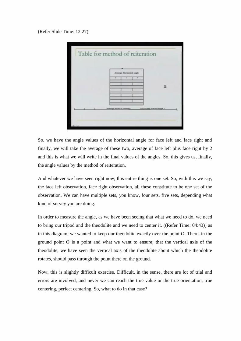
(Refer Slide Time: 12:27)
So, we have the angle values of the horizontal angle for face left and face right and
finally, we will take the average of these two, average of face left plus face right by 2
and this is what we will write in the final values of the angles. So, this gives us, finally,
the angle values by the method of reiteration.
And whatever we have seen right now, this entire thing is one set. So, with this we say,
the face left observation, face right observation, all these constitute to be one set of the
observation. We can have multiple sets, you know, four sets, five sets, depending what
kind of survey you are doing.
In order to measure the angle, as we have been seeing that what we need to do, we need
to bring our tripod and the theodolite and we need to center it. ((Refer Time: 04:43)) as
in this diagram, we wanted to keep our theodolite exactly over the point O. There, in the
ground point O is a point and what we want to ensure, that the vertical axis of the
theodolite, we have seen the vertical axis of the theodolite about which the theodolite
rotates, should pass through the point there on the ground.
Now, this is slightly difficult exercise. Difficult, in the sense, there are lot of trial and
errors are involved, and never we can reach the true value or the true orientation, true
centering, perfect centering. So, what to do in that case?

We should know, if at all we are introducing some errors due to miscentering, what kinds
of errors will be propagated into the angle that we measure. So, this is what we are going
to see now. We are going to see error in angle measurement due to miscentering.
(Refer Slide Time: 14:04)
So, basically, if I draw the diagram here, what it is like? Let us say, there are two points,
P and Q and O has to be here. This is the observer and we want to measure angle theta.
The meaning of miscentering is, somehow we are not able to center our instrument at O,
rather we are centering at O dash. Now, because of this what will happen? Instead of
taking OP and OQ as the line of sight, we will be taking O dash P and O dash Q as the
line of sights.
So, what we are doing? Instead of measuring theta, we are measuring phi. So, this error e
in angle due to theta minus phi or we can say, due to this miscentering, is the error
introduced in our angle. So, we can see by this simple diagram, that whenever we are
measuring the angles and if there is miscentering, there is some error, which is going to
be introduced in our angle measurement. Because there in the field what angle we need
to measure? In the field we need to measure theta because the angle in the field is theta.
But what we are measuring? We are measuring phi and because of this there is an error
of e here.
Now, what this e will depend upon? What it will depend upon, let us see. Number one, it
will depend upon the amount of e, how far is the miscentering. You know is the
miscentering is small or large? If it is smaller, this O dash point is somewhere here, then
the value of e will be small. It will also depend upon the length of lines of sight. What is
the meaning of this?
(Refer Slide Time: 16:29)
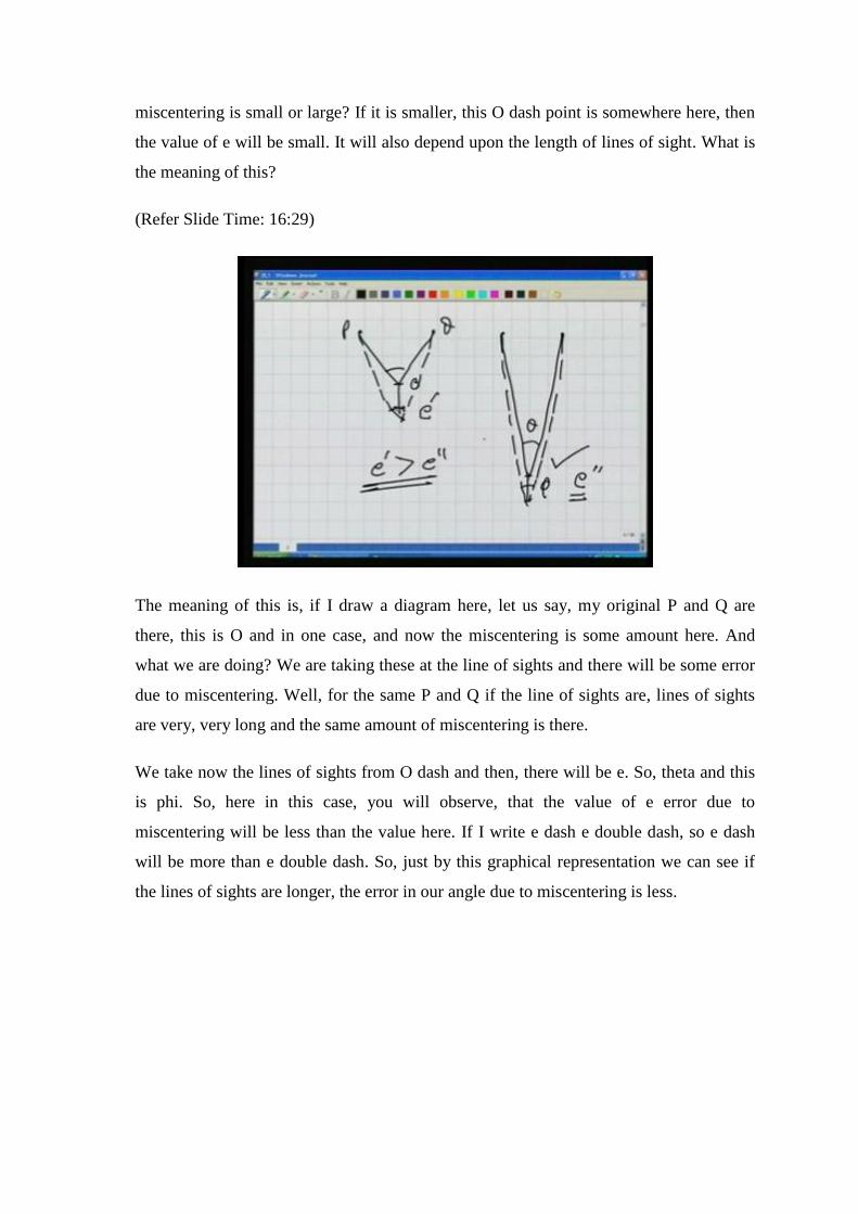
The meaning of this is, if I draw a diagram here, let us say, my original P and Q are
there, this is O and in one case, and now the miscentering is some amount here. And
what we are doing? We are taking these at the line of sights and there will be some error
due to miscentering. Well, for the same P and Q if the line of sights are, lines of sights
are very, very long and the same amount of miscentering is there.
We take now the lines of sights from O dash and then, there will be e. So, theta and this
is phi. So, here in this case, you will observe, that the value of e error due to
miscentering will be less than the value here. If I write e dash e double dash, so e dash
will be more than e double dash. So, just by this graphical representation we can see if
the lines of sights are longer, the error in our angle due to miscentering is less.

(Refer Slide Time: 17:53)
Anything else in which this error due to miscentering will depend upon? It also depends
upon the direction. The direction means, the miscentering could be in this direction or it
could be by same amount in this direction. Now, it can be proved very quickly, that the
error in the angle due to miscentering will be more if the miscentering is in the direction
of bifurcation of this angle. For example, in this direction, this, the miscentering error
will be maximum in this case than in any other case. It can be proved very quickly. We
have seen now two methods: method of repetition method of reiteration to measure any
angle.
(Refer Slide Time: 18:34)

What we can do? The angles, which are there in the field, as we have seen for example,
here each of these angles we can measure individually by method of repetition and also,
each of these angles can be measured by method of reiteration. Now, what we want to
see? We want to see in terms of accuracy, which of these method is better. So, for that
we need to do a little analysis and what we will do in this analysis we will revisit some of
the things which we had discussed in our earlier video lectures when we were talking
about the error propagation. We will see, we will do one analysis here how the error
propagates from a simple thing to a complex thing ((Refer Time: 19:19)) or in our final
measurement. This is what we will see. So, we will start with method of reiteration.
(Refer Slide Time: 19:28)
Now, in the method of reiteration, what we do, this is our P and Q, observer is here and
we measure this angle theta. How do we measure the angle theta? Theta is, basically,
given by D2 minus D1. What is D2 and D1? We are taking a back sight at P, we are
taking the foresight at Q and D2 and D1 are the averages. So, I can write the D2 as sigma
D2 i, I will explain this terms in a moment by n, and as well as D 1 as sigma D 1 i by n.
Now, why I am writing this in this way? Because here, as you see, theta is D2 minus D1.
The average of all the foresights minus the average of all the back sights, this is what we
do in reiteration, gives me the angle theta. Now, what is the single back sight or fore
sight. A single back sight or fore sight is when you are bisecting from O to P. What we

are doing? We are doing two things. Number one, we are doing the bisection and number
two, we are taking the reading, we are taking the observations.
(Refer Slide Time: 21:17)
Now, how this bisection and taking the reading will introduce error? Because when I am
bisecting, what is the meaning of bisection? For example, let us say, if there is a tree or
may be, for let us say, be there is a ranging rod here. Let us be more precise, because in
case of tree where to bisect will be something, you know, more of confusion.
Let us take a case of the ranging rod. Now, we want to bisect this ranging rod. So, what
we do? We put our field of view, this be something, which you are seeing through the
telescope on the ranging rod, and we align our cross hair with the center of the ranging
rod. So, this aligning of the cross hair with the center of the ranging rod is the bisection.
Now, the question is, can we really align it? Will there be some error? Yes, we can never
align it truly to the point or to the center of the ranging rod. So, there will be some error
because of the bisection. Second thing, once we have aligned it wherever, what we are
doing? We are taking the reading; we are taking the observation. So, while we take the
reading through our graduated circle what we do? We look through the Verniers and try
to see the reading. Again, this is also one more source of error. What about we read, we
cannot read the true value. No, we cannot read the true value.

(Refer Slide Time: 22:49)
So, they are error sources because of bisection and reading and these two errors can be
estimated. Let us say, the standard deviation for bisection error is sigma P square and the
standard deviation for reading error is sigma R square.
Now, as we have seen, we are, in the method of reiteration our D2 is average of all the
foresights. Now, what is one foresight? If you look at one foresight D2 i, this i varies
from 1 to n. The meaning of this is, there are n number of observations of the angle. This
angle we are observing n number of times. So, there are n number of foresights and n
number of back sights and this is how we are determining this angle. So, this i varies
from 1 to n.
Now, in any single foresight, let us say, in any single foresights the error of D2 i, the
standard deviation of this is depended upon and can be written as sigma R square plus
sigma P square because these two are the sources of error in taking the foresight. So, in
my foresight these two are the error sources. So, the standard deviation of the error for
this fore sight will be given by this formula.

(Refer Slide Time: 24:40)
Now, if it is so, what we are interested in? We are interested in finding D2 where D2 is
the mean D2 i by n.
Now, we have seen one formula. We have seen, that formula is, if Y is f(xi). We are
computing this Y from several observations, which are for example, x1, x2, x3, so on, up
to xn. So, in, by, in computing this particular quantity we are making use of all these
observations and in all these observations there are errors, sigma x1 square, sigma x2
square, sigma x3 square and so on.
For example, we know these. So, we have seen in the error propagation, that how these
individual errors will propagate into Y and this is given by, if you recall, sigma Y square
is sigma i is 1 to n because there are n number of variables and partial differentiation of
this function f against each of these i, square of this and multiplied by sigma xi square.
Now, this we have seen. Now, what we will try to do? We will try to use this for this
formula. Now, if it is so, what we are interested in? We are interested in square. Now,
how do we find it? So, the meaning is, if you take the note from here, we are going to
differentiate now this D2 partially with each individual D2 i according to this formula.
So, what it becomes?
(Refer Slide Time: 26:46)
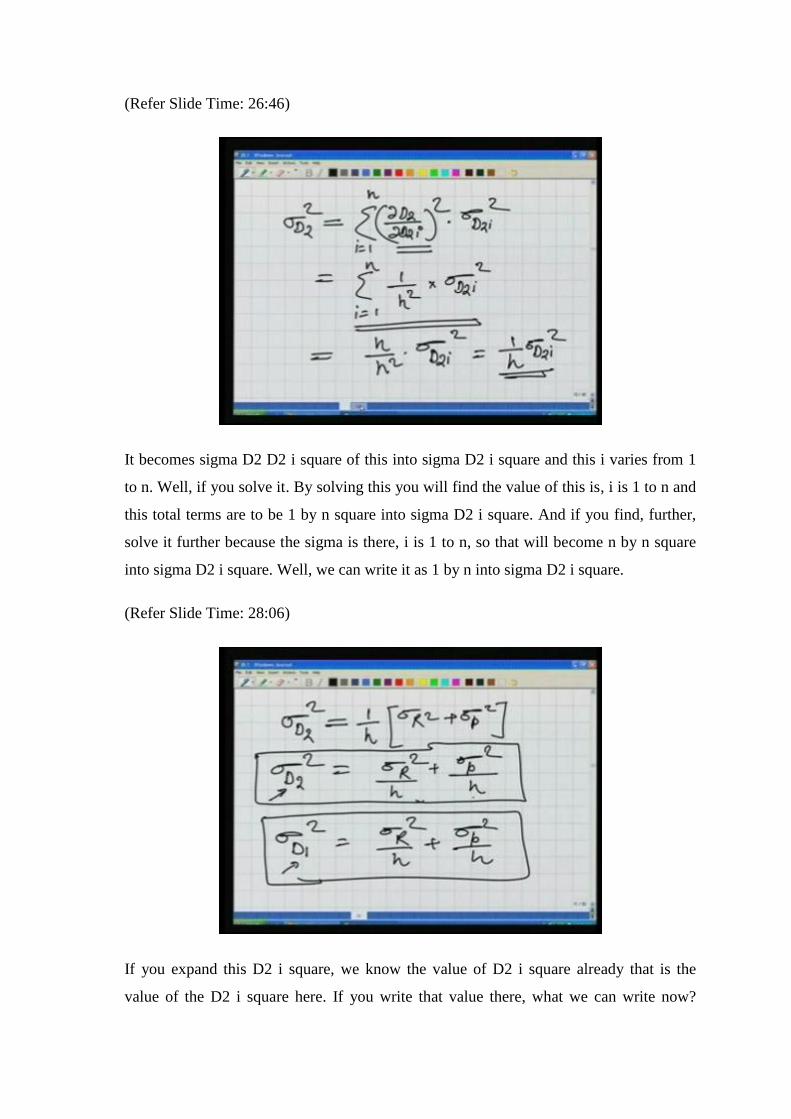
It becomes sigma D2 D2 i square of this into sigma D2 i square and this i varies from 1
to n. Well, if you solve it. By solving this you will find the value of this is, i is 1 to n and
this total terms are to be 1 by n square into sigma D2 i square. And if you find, further,
solve it further because the sigma is there, i is 1 to n, so that will become n by n square
into sigma D2 i square. Well, we can write it as 1 by n into sigma D2 i square.
(Refer Slide Time: 28:06)
If you expand this D2 i square, we know the value of D2 i square already that is the
value of the D2 i square here. If you write that value there, what we can write now?

Sigma D2 square is equal to 1 by n sigma R square plus sigma P square. So, that
becomes sigma R square plus divided by n sigma P square divided by n and that is my
D2 square. Let us look at this, what it is so for.
If you are looking at this, then you will notice the sigma D2 square is the error, which is
propagated because of the reading error and because of the bisection error in the average
of the foresight. Well, similarly with the, same we can write also sigma D1 square as
sigma R square divided by n plus sigma P square divided by n. Now, what is the
meaning of this because when we are taking the back sight that was D1, when we are
taking the foresight, D2. The things are same, there is no change. So, there is no change.
The error, which is propagated will be the same.
(Refer Slide Time: 29:44)
This is still not clear because we want to determine our theta and theta is D2 minus D1.
Now, the error, which is there in D2, which is sigma D2 square and the error, which is in
D1, sigma D1 square. We are writing these errors in terms of the standard deviations
here, how they propagate finally into theta.
So, in order do it again we will use what we had done for f(xi), that particular formula
we will use. In order to use that we can write sigma theta square as if we, part, partially
differentiate now this with D2 and D1 individually. We will find that it will be 1 into
sigma D2 square plus 1 into sigma D1 square.

So, if you write it further down because we know these values of sigma D2 square and
sigma D1 square, so if you write it further we can write it as 2 times now from here
sigma i square by n plus sigma p square by n. This sigma theta square is the error in
angle measurement for this theta in the case of the method of reiteration and it is being
given by this particular value here.
(Refer Slide Time: 31:33)
Now, what happens in case of method of repetition? If you look at the basis of the
method of repetition, in the case of the method of repetition, our observer is here, point P
and point Q, what we do? We first of all bisect P, the ranging rod there and we bisect and
we take the observation. Then, after doing several rounds of the instruments, several
rounds of the instrument because we are summing up the values mechanically. And then,
we finally take the reading here, take the reading at Q while in between when we are
doing these rounds, we always, at every time bisect Q.
So, what we are doing? We are doing the reading, we are taking the reading only twice,
only twice. Twice means, once at P and at last at Q while we are doing the bisection.
How many times we are doing the bisection? If for example, there are n number of
repetitions we are doing it 2n times. One at P, because initially, first of all we bisected P
and then, we are going to the Q, again bisecting it and again we are bisecting, again we
are bisecting and we keep bisecting that way. So, all these bisections are involved. So, 2n
number of bisections; the total number of bisections are 2n.

Now, how it is going to affect our angle theta? The angle theta, we write here as our final
reading D2 minus initial reading divided by number of the iterations that we have done.
(Refer Slide Time: 33:41)
.
Now, how the error will propagate again in this case again? Now, in the case of the D1,
what the D1 was? D1 is, we are taking a reading, we are taking one reading only, one
reading here and we are bisecting it and we are bisecting it, first reading and then we are
bisecting this one.
So, in the case of the D1 we can write it as the error in D1 will be sigma R square plus
sigma P square because D1 means, the very first reading. Very first reading means, we
are bisecting this P, we are bisecting it once and then we are taking the reading and that
is the value of D1; that gives us the value of D1. While in the case of the D2, what we
are doing in the case of the D2? For each D2, P and Q. So, for this Q what we are doing?
We come over here, we bisect it, we again close the horizon and again bisect it. So, one
more bisection now. Again, we, over here, one more bisection, we close the horizon, one
more bisection, again we come over here. So, bisection plus bisection and finally, after
doing this for n number of times, we do our final bisection and the reading.
So, we are taking the reading only at the last, but while we are doing this bisection, we
are bisection, bisecting P and then Q and then P, then Q, this is the procedure of
repetition. So, if it is so in the case of the D2, the error will be sigma R square plus 2n

minus 1 into sigma p square because we have, in order to take this D2 we have done only
one reading while we have done the bisections 2n minus 1 number of times. Well, what
we know in the case of the repetitions? The angle is given this way, theta is D2 minus D1
by n. We know now the error in D2 and error in D1, how they will propagate in theta.
So, this is what we are going to see because we know the error in D1 and error in D2.
(Refer Slide Time: 36:34)
So, error propagation in theta, because the theta we are writing as D2 minus D1 by n. So,
using again and sigma Y square we have done it, i is 1 to n, del f by del xi square into
sigma xi square. Using the same philosophy we can compute now for sigma theta square
and if you not differentiate partially, this particular function against D2 and D1, what we
will get? We will get 1 by n square sigma D2 square plus 1 by n square sigma D1 square.
Now, we put the value of D2 and D1 from here, sigma D1 square and sigma D2 square.
Sorry, I should write it as sigma D2 square is sigma R square plus 2n minus 1 sigma p
square.
Now, if I take these values here, so what kind, what I can do? I can write it as now 1 by n
square, I take it out, sigma R square plus 2n minus 1 into sigma P square plus for sigma
D1. Sigma D1 square is sigma R square plus sigma P square; sigma R square plus sigma
P square.

(Refer Slide Time: 38:35)
We solve it further now. In solving this further what we will find? We will find, that
sigma R square and sigma R square, they will add. So, we can write it further as sigma
theta square as 1 by n square sigma R square, I have got twice of that, plus 2n sigma P
square. Now, this can further be simplified as 2 sigma R square divided by n square plus
2 sigma P square divided by n, and this is what we get here. Now, we compare this with
the one, which we got for method of reiteration. In that case, we got R square by n plus 2
sigma P square by n. This is what we got in the cases of method of reiteration, as you can
see here.
(Refer Slide Time: 39:42)

Now, what is the meaning of this? Let us look into the meaning of this. In the case of the
method of repetition and reiteration, the error which is propagated into our final angle,
that we are writing, by sigma D square, the standard deviation of the error. In both the
cases, it is dependent upon the error due to the reading and the error due to bisection; the
error due to reading and the error due to bisection, similarly here.
However, as you will notice, for the reading the term here in the case of the repetition is
n square while in the case of reiteration it is n. What is the meaning of this? The error
propagated in theta is less in the case of the repetition because of the reading because the
term is square here and this term is only one.
So, what does it indicate? This indicates, because in the case of the repetition method we
are taking very few or rather only two number of readings, the first reading and the last
reading, so the error propagated in our final angle value because of the reading is less.
So, that means, the angles, which we compute or which we observe by repetition are
better than the angles, which we determine using the reiteration.
Now, this is very important and this analysis is very important and the steps, which are
involved in this analysis, you should do it yourself, then only you will understand all this
clearly.
(Refer Slide Time: 41:50)

So, far we have seen the methods for measuring angles in horizontal. Now, we will see
the method for measuring vertical angle. Now, what is the meaning of vertical angle?
The meaning of vertical angle is, for any object we are measuring the angle of this, from
the point of observer with the reference as the horizontal line. So, that is the horizontal
plane. So, from this horizontal plane we are measuring this angle to an object there. So,
that is my vertical angle. We have seen this definition.
How do we measure this using the theodolite? So, this is what we are going to see now
with the help of theodolite. Now, here in the theodolite, the procedure will be same,
some of the procedures as in the case of the horizontal angle. First of all, we take this
theodolite to a point where we need to measure the angle because obviously, whenever
we are measuring the angles, we are measuring the angles at the point of the observer
from a station. So, we will take this tripod there, we will center it, we will level it.
Now, once we have centered it, leveled it, we will fix this instrument, the theodolite, on
the tripod and again we will level using these three foot screws. So, the idea is to make
this horizontal plate horizontal.
Now, this is the horizontal. What it does, while we are leveling this instrument or the
theodolite using this foot screws and making this plate bubble in the center, it also
ensures, that my vertical circle is also vertical, which is important.
Henceforth, I am going to measure the angles in vertical plane, I do not want to measure
the angles in inclined plane. I want to measure them in a vertical plane, so my vertical
circle has to be vertical.

(Refer Slide Time: 43:38)
Well, one more thing, because in the case of the vertical angle measurement, that is, the
vertical circle and this is the Vernier or the index plane, what happens if I rotate, as we
do here? If I rotate my telescope, what is happening there in the case of the vertical
circle? It starts rotating with the rotation of the telescope. The vertical circle rotates, but
the index or the Vernier, they stay where they are. So, these index or these Vernier, they
form a line, which is the horizontal line or horizontal reference. So, I need to ensure, that
this is also horizontal.
(Refer Slide Time: 44:24)

How do we ensure it? We will make use of the altitude bubble. We have seen on the
index frame, there is an altitude bubble. This altitude bubble is more sensitive, more
sensitive than the plate bubble. So, after centering this plate bubble, again using the foot
screws we centered this altitude bubble.
Now, this is very interesting. I am saying the altitude bubble is more sensitive than the
plate bubble. Plate bubble is in center. Now, it is center wherever I rotate my instrument.
Now, I try to bring this in center. While I try to bring it in center, my plate bubble will
not change, will not shift its position because it is more sluggish than this one.
Well, once this altitude bubble is also in center, what it ensure? This ensure, that my
index is horizontal. Now, at that time when my index is horizontal, if I rotate my
telescope in such a way, that the reading over here in Vernier A, generally for the
vertical circle we say Vernier C and Vernier D, is 0, 0, 0. If it is so, my line of sight
should be horizontal.
I repeat, when, because my index is horizontal, now I make this, I rotate this telescope.
In order to ensure what is happening while I am rotating the telescope, the vertical circle
is rotating against the Vernier. I make the reading 0, 0, 0. We can make use of the
tangent screws and the clamp screw in order to do these things. So, once that is ensured,
that the reading is 0, 0, 0 here, 0, 0, 0 here, sorry, 180, 0, 0, 0, then in that case, the line
of sight, which we can see here should be horizontal.
Now, in order to measure the vertical angle what next we do? We sight to the object. Of
course, we will need to focus the eye piece and focus the objective lens, so that particular
object is bisected. Once that is bisected, whatever is the reading over here now in Vernier
C and Vernier D, we note down those readings and these give us the value of the vertical
angle. The vertical angle as defined here, the line going there, the horizontal line and the
angle here.

(Refer Slide Time: 46:56)
This we are doing right now for me in face right. So, we repeat this entire procedure on
the face left also.
(Refer Slide Time: 47:04)
How do we record these readings? We will come to the slide here. Now, this is the table
for vertical angle measurement. The instrument, as in the case, that is the point where
observer is. So, instrument is at O, our two points are P and Q to which we have to
measure the angles. So, P and Q that is the sight 2.

Right now, we are taking the observation, for example, in face left. Now, we are writing
the readings here in degrees, seconds and sorry, minutes and seconds. So, whatever was
the value of the reading we will write it here and this is for another Vernier, the Vernier
D, this is Vernier C and we take the mean of the each, mean of Vernier C and D. We
write the mean here and that gives us the vertical angle. Similarly, we do it for Q and it
will give us the vertical angle for Q also. So, vertical angle for Q, vertical angle for P.
We can do the same procedure on face right again reading the Vernier C and Vernier D,
taking the mean and finding the angle and then, finally the angle, which is coming from
the face left and the angle value, which is coming from the face right will average these
two and we will write the average of face left and face right. Similarly, for Q also
average of face left and face right.
So, what we have done? This is what is recorded here is for any object P only one set of
observation. We can repeat this multiple times depending, you know, how accurate we
want to be in our observations. So, this is how we observe the vertical angle.
Now, we have seen all these angle measurements, we are going to another aspect. What
are the errors? Are there any errors in measuring these angles? What are the errors,
which may be introduced into the theodolite? So, we will look into those errors now.
(Refer Slide Time: 50:40)

Now, in the errors in the theodolite, as usual, we will talk first about the personal errors.
How the personal errors will be introduced when we are doing the theodolite
measurement?
If you look at here, the observer, the surveyor has not done the leveling proper. If the
leveling is not proper, my horizontal circle is not horizontal. If my horizontal circle is not
horizontal, what is happening? Now, my graduated circle is inclined. So, all the
observations, all the angles, which are, which I am taking now horizontal angle, I am not
in horizontal plane, rather in inclined plane. Now, this could be one error, which can be
introduced by the observer. Miscentering, we have seen the effect of the miscentering,
what will happen. Then, the bisection is not proper. We need to bisect the object
properly. So, the bisection is not proper, again there may be error.
Error in the parallax, if the parallax is not removed, we have seen how the parallax can
be removed. If the parallax is not removed properly, again that will lead to the error in
the theodolite because of the surveyor. Finally, while he is taking the readings, he is not
taking the readings properly, again this is also a source of the error. So, these all are the
personal sources of the error.
Similarly, the natural errors. There may, there may be many, some of them, while we are
working in the field with the theodolite. It might happen if the ground is soft, one of the
legs goes down. So, what will happen? The level will, leveling will change and now our
observations will be wrong, or if it is too windy in the ground and there are vibrations in
the instrument, again the readings, which are taken will be wrong or may be, the
refractive index of the medium.
Many times in the summers you will see when you are looking through the theodolite or
the telescope, you will see there is simmering effect. Your ranging rod will appear to be
simmering. So, it becomes very difficult because of the natural condition, bisection of
the ranging rod becomes difficult. So, that also leads to the error.

(Refer Slide Time: 52:04)
One more error, for example, let the sun is on this side here. So, only part of the
instrument is being heated. Now, if only part of the instrument is being heated, what will
be the reason? What will, what might happen? The graduated circle may expand in one
part while it is not so in the other place. So, again that might lead to some error.
Also, that is my bubble tube here and the sun is shining from here, the sun light is falling
on the instrument. So, only part of the bubble tube is being heated. Because of that the
bubble will not remain in center, it will go out of the center. While we might constitute,
that the leveling has changed and we will try to level it so. In fact, what is happening?
We are changing the horizontal circle. We are not, it is not any more horizontal, we are
changing it to be inclined. So, because of these natural conditions also there might be
several errors, which might be added in the instrument.
Finally, the errors due to instrument, which we say, instrumental errors. Now, before we
get into the instrumental error we need to understand couple of fundamental lines of the
instrument. These are very, very important. We have understood the construction of the
instrument, how it is made and all these things, but we need to look into some of the
fundamental lines in this instrument.

(Refer Slide Time: 53:23)
When we are talking about the fundamental lines of the theodolite, you have to follow
the instructions of what I am showing you here very clearly where that will make you
understand what these lines are. We start with the vertical axis. If I rotate this theodolite,
it is rotating about an axis, which is the vertical axis of the theodolite.
So, we can show this as a line here, then this is the horizontal plate and the axis of the
bubble tube. If, if i showed in this diagram, this is the horizontal plate and that red line is
the axis of the bubble tube. There is some relationship. The relationship is, the horizontal
plate should be parallel to the axis of the bubble tube, they should be parallel to each
other. Then, as well as these two should be perpendicular to the line of, to the vertical
axis. As we can see here, these are perpendicular to the vertical axis.
Then, further we have now two axis system in this part of the instrument. One is for the
upper circle or the Vernier frame and the other one is for the bottom plate. Now, these
two axis again should coincide. As you can see here, by the dotted lines, that is what the
inner one and that is for the outer one. So, these two should coincide.
If you go further up, the lines one here is the horizontal axis, what is this. Now, in this
theodolite if I rotate my telescope, it is rotating about a line here, this line, we say, the
horizontal axis or trunnion axis. So, this is the horizontal axis or the trunnion axis. Is
there any relationship between vertical axis and this horizontal axis? Yes, they should be
perpendicular to each other.

As we can see here when we go further up, this blue line is the line of sight. So, the line,
which is passing through like this, if I rotate it, the line of sight is rotating, as well as
there is one more line, which is shown here by the dotted one. This is the line of
collimation. Ideally, the line of collimation and the line of sight should be coinciding as
well as these should be perpendicular to the horizontal axis and the vertical axis.
For example, here if I rotate it anywhere, the angle formed by line of sight to the
horizontal axis is 90 degree, as well as the angle formed by the horizontal axis with the
vertical axis is also 90 degree or we can say this way. So, these relationships should be
maintained in the instrument. If you go further up we have the vertical circle, that is, the
vertical circle. Now, the relationship of the vertical circle is this vertical circle should be
perpendicular to the horizontal axis or trunnion axis.
(Refer Slide Time: 56:19)
And we have the altitude bubble. So, this altitude bubble is in such a way, that once this
altitude bubble is at the center, the line formed by the index of Vernier should be
horizontal. So, this is what I am trying to show you here by this diagram. So, these all are
the various lines of a theodolite, which is a fundamental lines of the theodolite. So, what
we have seen? We have seen the inter relationships of these lines. When we discuss
further about the theodolite we will look into these lines again.
So, what we did today? We looked into the method of reiteration. We compared the
method of reiteration with method of repetition for their accuracies. We saw how to

measure the vertical angle, and then finally we have seen now the fundamental lines of a
theodolite, which we will again repeat in our coming lectures.
Thank you.