Survey Sampling - Berkeleyrice/Book3ed/p227.pdf · Survey Sampling 7.1 Introduction ... for example, the U.S. government con- ... 7.3.1 The Expectation and Variance of the Sample

Rice-15149 book March 16, 2006 12:53

C H A P T E R 7

Survey Sampling

7.1 IntroductionResting on the probabilistic foundations of the preceding chapters, this chapter marksthe beginning of our study of statistics by introducing the subject of survey sampling.As well as being of considerable intrinsic interest and practical utility, the developmentof the elementary theory of survey sampling serves to introduce several concepts andtechniques that will recur and be amplified in later chapters.

Sample surveys are used to obtain information about a large population by exam-ining only a small fraction of that population. Sampling techniques have been usedin many fields, such as the following:

• Governments survey human populations; for example, the U.S. government con-ducts health surveys and census surveys.

• Sampling techniques have been extensively employed in agriculture to estimatesuch quantities as the total acreage of wheat in a state by surveying a sample offarms.

• The Interstate Commerce Commission has carried out sampling studies of rail andhighway traffic. In one such study, records of shipments of household goods bymotor carriers were sampled to evaluate the accuracy of preshipment estimates ofcharges, claims for damages, and other variables.

• In the practice of quality control, the output of a manufacturing process may besampled in order to examine the items for defects.

• During audits of the financial records of large companies, sampling techniques maybe used when examination of the entire set of records is impractical.

The sampling techniques discussed here are probabilistic in nature—each mem-ber of the population has a specified probability of being included in the sample, andthe actual composition of the sample is random. Such techniques differ markedly from

199

Rice-15149 book March 16, 2006 12:53

200 Chapter 7 Survey Sampling

the type of sampling scheme in which particular population members are includedin the sample because the investigator thinks they are typical in some way. Such ascheme may be effective in some situations, but there is no way mathematically toguarantee its unbiasedness (a term that will be precisely defined later) or to estimatethe magnitude of any error committed, such as that arising from estimating the popu-lation mean by the sample mean. We will see that using a random sampling techniquehas a consequence that estimates can be guaranteed to be unbiased and probabilisticbounds on errors can be calculated. Among the advantages of using random samplingare the following:

• The selection of sample units at random is a guard against investigator biases, evenunconscious ones.

• A small sample costs far less and is much faster to survey than a complete enumer-ation.

• The results from a small sample may actually be more accurate than those from acomplete enumeration. The quality of the data in a small sample can be more easilymonitored and controlled, and a complete enumeration may require a much larger,and therefore perhaps more poorly trained, staff.

• Random sampling techniques make possible the calculation of an estimate of theerror due to sampling.

• In designing a sample, it is frequently possible to determine the sample size neces-sary to obtain a prescribed error level.

Peck et al. (2005) contains several interesting papers about applications ofsampling.

7.2 Population ParametersThis section defines those numerical characteristics, or parameters, of the populationthat we will estimate from a sample. We will assume that the population is of sizeN and that associated with each member of the population is a numerical value ofinterest. These numerical values will be denoted by x1, x2, · · ·, xN . The variable xi

may be a numerical variable such as age or weight, or it may take on the value 1 or0 to denote the presence or absence of some characteristic such as gender. We willrefer to the latter situation as the dichotomous case.

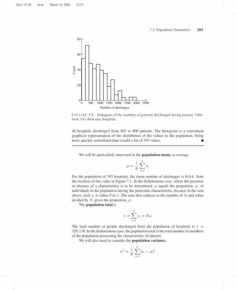
E X A M P L E A This is the first of many examples in this chapter in which we will illustrate ideasby using a study by Herkson (1976). The population consists of N = 393 short-stay hospitals. We will let xi denote the number of patients discharged from the i thhospital during January 1968. A histogram of the population values is shown in Fig-ure 7.1. The histogram was constructed in the following way: The number of hospitalsthat discharged 0–200, 201– 400, . . . , 2801–3000 patients were graphed as horizon-tal lines above the respective intervals. For example, the figure indicates that about

Rice-15149 book March 16, 2006 12:53

7.2 Population Parameters 201

0500 1000 1500 2000

Cou

nt

Number of discharges

20

40

60

80

0 2500 35003000

F I G U R E 7.1 Histogram of the numbers of patients discharged during January 1968from 393 short-stay hospitals.

40 hospitals discharged from 601 to 800 patients. The histogram is a convenientgraphical representation of the distribution of the values in the population, beingmore quickly assimilated than would a list of 393 values. ■

We will be particularly interested in the population mean, or average,

µ = 1

N

N∑i=1

xi

For the population of 393 hospitals, the mean number of discharges is 814.6. Notethe location of this value in Figure 7.1. In the dichotomous case, where the presenceor absence of a characteristic is to be determined, µ equals the proportion, p, ofindividuals in the population having the particular characteristic, because in the sumabove, each xi is either 0 or 1. The sum thus reduces to the number of 1s and whendivided by N , gives the proportion, p.

The population total is

τ =N∑

i=1

xi = Nµ

The total number of people discharged from the population of hospitals is τ =320,138. In the dichotomous case, the population total is the total number of membersof the population possessing the characteristic of interest.

We will also need to consider the population variance,

σ 2 = 1

N

N∑i=1

(xi − µ)2

Rice-15149 book March 16, 2006 12:53


A useful identity can be obtained by expanding the square in this equation:

σ 2 = 1

N

(N∑

i=1

x2i − 2µ

N∑i=1

xi + Nµ2

)

= 1

N

(N∑

i=1

x2i − 2Nµ2 + Nµ2

)

= 1

N

N∑i=1

x2i − µ2

In the dichotomous case, the population variance reduces to p(1 − p):

σ 2 = 1

N

N∑i=1

x2i − µ2

= p − p2

= p(1 − p)

Here we used the fact that because each xi is 0 or 1, each x2i is also 0 or 1.

The population standard deviation is the square root of the population varianceand is used as a measure of how spread out, dispersed, or scattered the individual valuesare. The standard deviation is given in the same units (for example, inches) as are thepopulation values, whereas the variance is given in those units squared. The varianceof the discharges is 347,766, and the standard deviation is 589.7; examination ofthe histogram in Figure 7.1 makes it clear that the latter number is the more reasonabledescription of the spread of the population values.

7.3 Simple Random SamplingThe most elementary form of sampling is simple random sampling (s.r.s.): Eachparticular sample of size n has the same probability of occurrence; that is, each of the(N

n

)possible samples of size n taken without replacement has the same probability.

We assume that sampling is done without replacement so that each member of thepopulation will appear in the sample at most once. The actual composition of thesample is usually determined by using a table of random numbers or a random numbergenerator on a computer. Conceptually, we can regard the population members asballs in an urn, a specified number of which are selected for inclusion in the sampleat random and without replacement.

Because the composition of the sample is random, the sample mean is random.An analysis of the accuracy with which the sample mean approximates the populationmean must therefore be probabilistic in nature. In this section, we will derive somestatistical properties of the sample mean.

Rice-15149 book March 16, 2006 12:53

7.3 Simple Random Sampling 203

7.3.1 The Expectation and Variance of the Sample MeanWe will denote the sample size by n (n is less than N ) and the values of the samplemembers by X1, X2, . . . , Xn . It is important to realize that each Xi is a random vari-able. In particular, Xi is not the same as xi : Xi is the value of the i th member of the sam-ple, which is random and xi is that of the i th member of the population, which is fixed.

We will consider the sample mean,

X = 1

n

n∑i=1

Xi

as an estimate of the population mean. As an estimate of the population total, we willconsider

T = N X

Properties of T will follow readily from those of X . Since each Xi is a randomvariable, so is the sample mean; its probability distribution is called its samplingdistribution. In general, any numerical value, or statistic, computed from a randomsample is a random variable and has an associated sampling distribution. The samplingdistribution of X determines how accurately X estimates µ; roughly speaking, themore tightly the sampling distribution is centered on µ, the better the estimate.

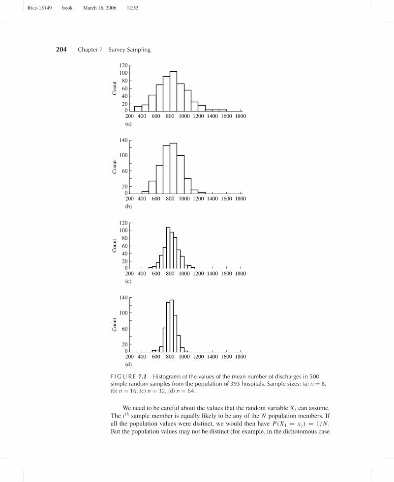
E X A M P L E A To illustrate the concept of a sampling distribution, let us look again at the populationof 393 hospitals. In practice, of course, the population would not be known, and onlyone sample would be drawn. For pedagogical purposes here, we can consider thesampling distribution of the sample mean from this known population. Suppose, forexample, that we want to find the sampling distribution of the mean of a sample of size16. In principle, we could form all

(39316

)samples and compute the mean of each one—

this would give the sampling distribution. But because the number of such samples isof the order 1033, this is clearly not practical. We will thus employ a technique knownas simulation. We can estimate the sampling distribution of the mean of a sample ofsize n by drawing many samples of size n, computing the mean of each sample, andthen forming a histogram of the collection of sample means. Figure 7.2 shows theresults of such a simulation for sample sizes of 8, 16, 32, and 64 with 500 replicationsfor each sample size. Three features of Figure 7.2 are noteworthy:

1. All the histograms are centered about the population mean, 814.6.2. As the sample size increases, the histograms become less spread out.3. Although the shape of the histogram of population values (Figure 7.1) is not

symmetric about the mean, the histograms in Figure 7.2 are more nearly so.

These features will be explained quantitatively. ■

As we have said, X is a random variable whose distribution is determined bythat of the Xi . We thus examine the distribution of a single sample element, Xi . Itshould be noted that the following lemma holds whether sampling is with or withoutreplacement.

Rice-15149 book March 16, 2006 12:53


020

400 600 800 1000C

ount

4060

80

100

200 1200

120

(a)1400 1600 1800

020

400 600 800 1000

Cou

nt

60

100

200 1200(b)

1400 1600 1800

020

400 600 800 1000

Cou

nt

4060

80

100

200 1200

120

(c)1400 1600 1800

140

020

400 600 800 1000

Cou

nt

60

100

200 1200(d)

1400 1600 1800

140

F I G U R E 7.2 Histograms of the values of the mean number of discharges in 500simple random samples from the population of 393 hospitals. Sample sizes: (a) n = 8,(b) n = 16, (c) n = 32, (d) n = 64.

We need to be careful about the values that the random variable Xi can assume.The i th sample member is equally likely to be any of the N population members. Ifall the population values were distinct, we would then have P(X1 = x j ) = 1/N .But the population values may not be distinct (for example, in the dichotomous case

Rice-15149 book March 16, 2006 12:53


there are only two values, 0 and 1). If k members of the population have the samevalue ζ , then P(Xi = ζ ) = k/N . We use this construction in proving the followinglemma.

L E M M A A

Denote the distinct values assumed by the population members by ζ1, ζ2, . . . , ζm,

and denote the number of population members that have the value ζ j by n j , j =1, 2, . . . , m. Then Xi is a discrete random variable with probability massfunction

P(Xi = ζ j ) = n j

NAlso,

E(Xi ) = µ

Var(Xi ) = σ 2

Proof

The only possible values that Xi can assume are ζ1, ζ2, . . . , ζm . Since each mem-ber of the population is equally likely to be the i th member of the sample, theprobability that Xi assumes the value ζ j is thus n j/N . The expected value of therandom variable Xi is then

E(Xi ) =m∑

j=1

ζ j P(Xi = ζ j ) = 1

N

m∑j=1

n jζ j = µ

The last equation follows because n j population members have the value ζ j

and the sum is thus equal to the sum of the values of all the population members.Finally,

Var(Xi ) = E(

X 2i

) − [E(Xi )]2

= 1

N

m∑j=1

n jζ2j − µ2

= σ 2

Here we have used the fact that∑

Ni=1x2

i = ∑mj=1n jζ

2j and the identity for the

population variance derived in Section 7.2. ■

As a measure of the center of the sampling distribution, we will use E(X). As ameasure of the dispersion of the sampling distribution about this center, we will usethe standard deviation of X . The key results that will be obtained shortly are that thesampling distribution is centered at µ and that its spread is inversely proportional tothe square root of the sample size, n. We first show that the sampling distribution iscentered at µ.

Rice-15149 book March 16, 2006 12:53


T H E O R E M A

With simple random sampling, E(X) = µ.

Proof

Since, from Lemma A, E(Xi ) = µ, it follows from Theorem A in Section 4.1.2that

E(X) = 1

n

n∑i=1

E(Xi ) = µ ■

From Theorem A, we have the following corollary.

C O R O L L A R Y A

With simple random sampling, E(T ) = τ.

Proof

E(T ) = E(N X)

= N E(X)

= Nµ

= τ ■

In the dichotomous case, µ = p, and X is the proportion of the sample thatpossesses the characteristic of interest. In this case, X will be denoted by p. We haveshown that E( p) = p.

It is important to keep in mind that X is random. The result E(X) = µ can beinterpreted to mean that “on the average” X = µ. In general, if we wish to estimatea population parameter, θ say, by a function θ of the sample, X1, X2, . . . , Xn , andE(θ) = θ , whatever the value of θ may be, we say that θ is unbiased. Thus, Xand T are unbiased estimates of µ and τ . On average they are correct. We nextinvestigate how variable they are, by deriving their variances and standard deviations.Section 4.2.1 introduced the concepts of bias and variance in the context of a modelof measurement error, and these concepts are also relevant in this new context. InChapter 4, it was shown that

Mean squared error = variance + bias2

Since X and T are unbiased, their mean squared errors are equal to their variances.We next find Var(X). Since X = n−1

∑ni=1 Xi , it follows from Corollary A of

Section 4.3 that

Var(X) = 1

n2

n∑i=1

n∑j=1

Cov(Xi , X j )

Rice-15149 book March 16, 2006 12:53


Suppose that sampling were done with replacement. Then the Xi would be inde-pendent, and for i �= j we would have Cov(Xi , X j ) = 0, whereas Cov(Xi , Xi ) =Var(Xi ) = σ 2. It would then follow that

Var X = 1

n2

n∑i=1

Var(Xi )

= σ 2

n

and that the standard deviation of X , also called its standard error, would be

σX = σ√n

Sampling without replacement induces dependence among the Xi , which com-plicates this simple result. However, we will see that if the sample size n is smallrelative to the population size N , the dependence is weak and this simple result holdsto a good approximation.

To find the variance of the sample mean in sampling without replacement weneed to find Cov(Xi , X j ) for i �= j .

L E M M A B

For simple random sampling without replacement,

Cov(Xi , X j ) = −σ 2/(N − 1) if i �= j

Using the identity for covariance established at the beginning of Section 4.3,

Cov(Xi , X j ) = E(Xi X j ) − E(Xi )E(X j )

and

E(Xi X j ) =m∑

k=1

m∑l=1

ζkζl P(Xi = ζk and X j = ζl)

=m∑

k=1

ζk P(Xi = ζk)

m∑l=1

ζl P(X j = ζl |Xi = ζk)

from the multiplication law for conditional probability. Now,

P(X j = ζl |Xi = ζk) ={

nl/(N − 1), if k �= l(nl − 1)/(N − 1), if k = l

Now if we expressm∑

l=1

ζl P(X j = ζl |Xi = ζk) =∑l �=k

ζlnl

N − 1+ ζk

nk − 1

N − 1

=m∑

l=1

ζlnl

N − 1− ζk

1

N − 1

Rice-15149 book March 16, 2006 12:53


the expression for E(Xi X j ) becomesm∑

k=1

ζknk

N

(m∑

l=1

ζlnl

N − 1− ζk

N − 1

)= 1

N (N − 1)

(τ 2 −

m∑k=1

ζ 2k nk

)

= τ 2

N (N − 1)− 1

N (N − 1)

m∑k=1

ζ 2k nk

= Nµ2

N − 1− 1

N − 1(µ2 + σ 2)

= µ2 − σ 2

N − 1

Finally, subtracting E(Xi )E(X j ) = µ2 from the last equation, we have

Cov(Xi , X j ) = − σ 2

N − 1for i �= j . ■

(Alternative proofs of Lemma B are outlined in Problems 25 and 26 at the end ofthis chapter.) This lemma shows that Xi and X j are not independent of each other fori �= j , but that the covariance is very small for large values of N . We are now able toderive the following theorem.

T H E O R E M B

With simple random sampling,

Var(X) = σ 2

n

(N − n

N − 1

)

= σ 2

n

(1 − n − 1

N − 1

)

Proof

From Corollary A of Section 4.3,

Var(X) = 1

n2

n∑i=1

n∑j=1

Cov(Xi , X j )

= 1

n2

n∑i=1

Var(Xi ) + 1

n2

n∑i=1

∑j �=i

Cov(Xi , X j )

= σ 2

n− 1

n2n(n − 1)

σ 2

N − 1After some algebra, this gives the desired result. ■

Rice-15149 book March 16, 2006 12:53


Notice that the variance of the sample mean in sampling without replacementdiffers from that in sampling with replacement by the factor(

1 − n − 1

N − 1

)

which is called the finite population correction. The ratio n/N is called the samplingfraction. Frequently, the sampling fraction is very small, in which case the standarderror (standard deviation) of X is

σX ≈ σ√n

We see that, apart from the usually small finite population correction, the spread of thesampling distribution and therefore the precision of X are determined by the samplesize (n) and not by the population size (N ). As will be made more explicit later,the appropriate measure of the precision of the sample mean is its standard error,which is inversely proportional to the square root of the sample size. Thus, in orderto double the accuracy, the sample size must be quadrupled. (You might examineFigure 7.2 with this in mind.) The other factor that determines the accuracy of thesample mean is the population standard deviation, σ . If σ is small, the populationvalues are not very dispersed and a small sample will be fairly accurate. But if thevalues are widely dispersed, a much larger sample will be required in order to attainthe same accuracy.

E X A M P L E B If the population of hospitals is sampled without replacement and the sample size isn = 32,

σX = σ√n

√1 − n − 1

N − 1

= 589.7√32

√1 − 31

392

= 104.2 × .96

= 100.0

Notice that because the sampling fraction is small, the finite population correctionmakes little difference. To see that σX = 100.0 is a reasonable measure of accuracy,examine part (b) of Figure 7.2 and observe that the vast majority of sample meansdiffered from the population mean (814) by less than two standard errors; i.e., thevast majority of sample means were in the interval (614, 1014). ■

E X A M P L E C Let us apply this result to the problem of estimating a proportion. In the population ofhospitals, a proportion p = .654 had fewer than 1000 discharges. If this proportionwere estimated from a sample as the sample proportion p, the standard error of p

Rice-15149 book March 16, 2006 12:53


could be found by applying Theorem B to this dichotomous case:

σ p =√

p(1 − p)

n

√1 − n − 1

N − 1

For example, for n = 32, the standard error of p is

σ p =√

.654 × .346

32

√1 − 31

392= .08 ■

The precision of the estimate of the population total does depend on the populationsize, N .

C O R O L L A R Y B


Var(T ) = N 2

(σ 2

n

)N − n

N − 1

Proof

Since T = N X ,

Var(T ) = N 2 Var(X) ■

7.3.2 Estimation of the Population VarianceA sample survey is used to estimate population parameters, and it is desirable alsoto assess and quantify the variability of the estimates. In the previous section, wesaw how the standard error of an estimate may be determined from the sample sizeand the population variance. In practice, however, the population variance will notbe known, but as we will show in this section, it can be estimated from the sample.Since the population variance is the average squared deviation from the populationmean, estimating it by the average squared deviation from the sample mean seemsnatural:

σ 2 = 1

n

n∑i=1

(Xi − X)2

Rice-15149 book March 16, 2006 12:53


The following theorem shows that this estimate is biased.

T H E O R E M A


E(σ 2) = σ 2

(n − 1

n

)N

N − 1

Proof

Expanding the square and proceeding as in the identity for the population variancein Section 7.2, we find

σ 2 = 1

n

n∑i=1

X 2i − X 2

Thus,

E(σ 2) = 1

n

n∑i=1

E(

X 2i

) − E(X 2)

Now, we know that

E(

X 2i

) = Var(Xi ) + [E(Xi )]2

= σ 2 + µ2

Similarly, from Theorems A and B of Section 7.3.1,

E(X 2) = Var(X) + [E(X)]2

= σ 2

n

(1 − n − 1

N − 1

)+ µ2

Substituting these expressions for E(X 2i ) and E(X 2) in the preceding equation

for E(σ 2) gives the desired result. ■

Because N > n, it follows with a little algebra that

n − 1

n

N

N − 1< 1

so that E(σ 2) < σ 2; σ 2 thus tends to underestimate σ 2. From Theorem A, we seethat an unbiased estimate of σ 2 may be obtained by multiplying σ 2 by the factorn(N −1)/[(n−1)N ]. Thus, an unbiased estimate of σ 2 is 1

n−1 (1− 1N )

∑ni=1(Xi − X)2.

We also have the following corollary.

Rice-15149 book March 16, 2006 12:53


C O R O L L A R Y A

An unbiased estimate of Var(X) is

s2X

= σ 2

n

(n

n − 1

) (N − 1

N

) (N − n

N − 1

)

= s2

n

(1 − n

N

)where

s2 = 1

n − 1

n∑i=1

(Xi − X)2

Proof

Since

Var(X) = σ 2

n

(N − n

N − 1

)

an unbiased estimate of Var(X) may be obtained by substituting in an unbiasedestimate of σ 2. Algebra then yields the desired result. ■

Similarly, an unbiased estimate of the variance of T , the estimator of the popu-lation total, is

s2T = N 2s2

X

For the dichotomous case, in which each Xi is 0 or 1, note that

1

n

n∑i=1

(Xi − X)2 = 1

n

n∑i=1

X 2i − X

2

= p(1 − p)

Therefore,

s2 = n

n − 1p(1 − p)

Thus, as a special case of Corollary A, we have the following corollary.

C O R O L L A R Y B

An unbiased estimate of Var( p) is

s2p = p(1 − p)

n − 1

(1 − n

N

)■

In many cases, the sampling fraction, n/N , is small and may be neglected. Fur-thermore, it often makes little difference whether n − 1 or n is used as the divisor.

Rice-15149 book March 16, 2006 12:53


The quantities sX , sT , and sp are called estimated standard errors. If we knewthem, the actual standard errors, σX , σT and σ p, would be used to gauge the accuracyof the estimates X , T and p. If they are not known, which is the typical case, theestimated standard errors are used in their place.

E X A M P L E A A simple random sample of 50 of the 393 hospitals was taken. From this sample,X = 938.5 (recall that, in fact, µ = 814.6) and s = 614.53 (σ = 590). An estimateof the variance of X is

s2X

= s2

n

(1 − n

N

)= 6592

The estimated standard error of X is

sX = 81.19

(Note that the true value is σX = σ√50

√1 − 49

392 = 78.) This estimated standard error

gives a rough idea of how accurate the value of X is; in this case, we see that themagnitude of the error is of the order 80, as opposed to 8 or 800, say. In fact, the errorwas 123.9, or about 1.5 sX . ■

E X A M P L E B From the same sample, the estimate of the total number of discharges in the populationof hospitals is

T = N X = 368,831

Recall that the true value of the population total is 320,139. The estimated standarderror of T is

sT = NsX = 31,908

Again, this estimated standard error can be used as a rough gauge of the estimationerror. ■

E X A M P L E C Let p be the proportion of hospitals that had fewer than 1000 discharges—that is,p = .654. In the sample of Example A, 26 of 50 hospitals had fewer than 1000discharges, so

p = 26

50= .52

The variance of p is estimated by

s2p = p(1 − p)

n − 1

(1 − n

N

)= .0045

Thus, the estimated standard error of p is

sp = .067

Rice-15149 book March 16, 2006 12:53


Crudely, this tells us that the error of p is in the second or first decimal place—thatwe are probably not so fortunate as to have an error only in the third decimal place.In fact, the error was .134 or about 2 × sp. ■

These examples show how, in simple random sampling, we can not only formestimates of unknown population parameters, but can also gauge the likely size of theerrors of the estimates, by estimating their standard errors from the data in the sample.

We have covered a lot of ground, and the presence of the finite population cor-rection complicates the expressions we have derived. It is thus useful to summarizeour results in the following table:

PopulationParameter Estimate Variance of Estimate Estimated Variance

µ X = 1n

∑ni=1 Xi σ 2

X= σ 2

n

(N−nN−1

)s2

X= s2

n

(1 − n

N

)p p = sample proportion σ 2

p = p(1−p)

n

(N−nN−1

)s2

p = p(1− p)

n−1

(1 − n

N

)τ T = N X σ 2

T = N 2σ 2X

s2T = N 2s2

X

σ 2(

1 − 1N

)s2

where s2 = 1n−1

∑ni=1(Xi − X)2.

The square roots of the entries in the third column are called standard errors,and the square roots of the entries in the fourth column are called estimated standarderrors. The former depend on unknown population parameters, so the latter are usedto gauge the accuracy of the parameter estimates. When the population is large relativeto the sample size, the finite population correction can be ignored, simplifying thepreceding expressions.

7.3.3 The Normal Approximation to the SamplingDistribution of XWe have found the mean and the standard deviation of the sampling distribution of X .Ideally, we would like to know the sampling distribution, since it would tell us every-thing we could hope to know about the accuracy of the estimate. Without knowledgeof the population itself, however, we cannot determine the sampling distribution. Inthis section, we will use the central limit theorem to deduce an approximation tothe sampling distribution—the normal, or Gaussian, distribution. This approximationwill be used to find probabilistic bounds for the estimation error.

In Section 5.3, we considered a sequence of independent and identically dis-tributed (i.i.d.) random variables, X1, X2, . . . having the common mean and varianceµ and σ 2. The sample mean of X1, X2, . . . , Xn is

Xn = 1

n

n∑i=1

Xi

Rice-15149 book March 16, 2006 12:53


This sample mean has the properties

E(Xn) = µ

and

Var(Xn) = σ 2

nThe central limit theorem says that, for a fixed number z,

P

(Xn − µ

σ/√

n≤ z

)→ �(z) as n → ∞

where � is the cumulative distribution function of the standard normal distribution.Using a more compact and suggestive notation, we have

P

(Xn − µ

σXn

≤ z

)→ �(z)

The context of survey sampling is not exactly like that of the central limit theoremas stated above—as we have seen, in sampling without replacement, the Xi are notindependent of each other, and it makes no sense to have n tend to infinity while Nremains fixed. But other central limit theorems have been proved that are appropriateto the sampling context. These show that if n is large, but still small relative to N ,then Xn , the mean of a simple random sample, is approximately normally distributed.

To demonstrate the use of the central limit theorem, we will apply it to approx-imate P(|X − µ| ≤ δ), the probability that the error made in estimating µ by X isless than some constant δ

P(|X − µ| ≤ δ) = P(−δ ≤ X − µ ≤ δ)

= P

(− δ

σX

≤ X − µ

σX

≤ δ

σX

)

≈ �

(δ

σX

)− �

(− δ

σX

)

= 2�

(δ

σX

)− 1

since �(−z) = 1 − �(z), from the symmetry of the standard normal distributionabout zero.

E X A M P L E A Let us again consider the population of 393 hospitals. The standard deviation of themean of a sample of size n = 64 is, using the finite population correction,

σX = σ√n

√1 − n − 1

N − 1

= 589.7

8

√1 − 63

392= 67.5

We can use the central limit theorem to approximate the probability that thesample mean differs from the population mean by more than 100 in absolute value; i.e.,

Rice-15149 book March 16, 2006 12:53


P(|X − µ| > 100). First, from the symmetry of the normal distribution,

P(|X − µ| > 100) ≈ 2P(X − µ > 100)

andP(X − µ > 100) = 1 − P(X − µ < 100)

= 1 − P

(X − µ

σX

<100

σX

)

≈ 1 − �

(100

67.5

)= .069

Thus the probability that the sample mean differs from the population mean by morethan 100 is approximately .14. In fact, among the 500 samples of size 64 in ExampleA in Section 7.3.1, 82, or 16.4%, differed by more than 100 from the population mean.Similarly, the central limit theorem approximation gives .026 as the probability ofdeviations of more than 150 from the population mean. In the simulation in ExampleA in Section 7.3.1, 11 of 500, or 2.2%, differed by more than 150. If we are not toofinicky, the central limit theorem gives us reasonable and useful approximations. ■

E X A M P L E B For a sample of size 50, the standard error of the sample mean number of dischargesis

σX = 78

For the particular sample of size 50 discussed in Example A in Section 7.3.2, wefound X = 938.35, so X − µ = 123.9. We now calculate an approximation of theprobability of an error this large or larger:

P(|X − µ| ≥ 123.9) = 1 − P(|X − µ| < 123.9)

≈ 1 −[

2�

(123.9

78

)− 1

]= 2 − 2�(1.59)

= .11

Thus, we can expect an error this large or larger to occur about 11% of the time. ■

E X A M P L E C In Example C in Section 7.3.2, we found from the sample of size 50 an estimatep = .52 of the proportion of hospitals that discharged fewer than 1000 patients; infact, the actual proportion in the population is .65. Thus, | p − p | = .13. What is theprobability that an estimate will be off by an amount this large or larger?

We have

σ p =√

p(1 − p)

n

√1 − n − 1

N − 1= .068 × .94 = .064

Rice-15149 book March 16, 2006 12:53


We can therefore calculate

P(|p − p| > .13) = 1 − P(|p − p| ≤ .13)

= 1 − P

( |p − p|σ p

≤ .13

σ p

)≈ 2[1 − �(2.03)] = .04

We see that the sample was rather “unlucky”—an error this large or larger wouldoccur only about 4% of the time. ■

We can now derive a confidence interval for the population mean, µ. A confi-dence interval for a population parameter, θ , is a random interval, calculated from thesample, that contains θ with some specified probability. For example, a 95% confi-dence interval for µ is a random interval that contains µ with probability .95; if wewere to take many random samples and form a confidence interval from each one,about 95% of these intervals would contain µ. If the coverage probability is 1 − α,the interval is called a 100(1 − α)% confidence interval. Confidence intervals arefrequently used in conjunction with point estimates to convey information about theuncertainty of the estimates.

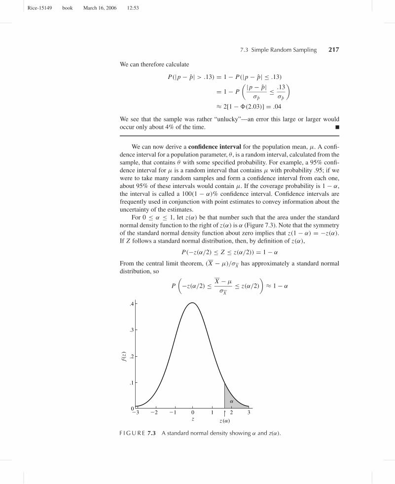
For 0 ≤ α ≤ 1, let z(α) be that number such that the area under the standardnormal density function to the right of z(α) is α (Figure 7.3). Note that the symmetryof the standard normal density function about zero implies that z(1 − α) = −z(α).

If Z follows a standard normal distribution, then, by definition of z(α),

P(−z(α/2) ≤ Z ≤ z(α/2)) = 1 − α

From the central limit theorem, (X − µ)/σX has approximately a standard normaldistribution, so

P

(−z(α/2) ≤ X − µ

σX

≤ z(α/2)

)≈ 1 − α

0

.1

�2 �1 0 1

f(z)

z

.2

.3

.4

�3 2

�

3

z (�)

F I G U R E 7.3 A standard normal density showing α and z(α).

Rice-15149 book March 16, 2006 12:53


Elementary manipulation of the inequalities gives

P(X − z(α/2)σX ≤ µ ≤ X + z(α/2)σX ) ≈ 1 − α

That is, the probability that µ lies in the interval X ± z(α/2)σX is approximately1 − α. The interval is thus called a 100(1 − α)% confidence interval. It is importantto understand that this interval is random and that the preceding equation states thatthe probability that this random interval covers µ is 1 −α. In practice, α is assigned asmall value, such as .1, .05, or .01, so that the probability that the interval covers µ willbe large. Also, since the population variance is typically not known, sX is substitutedfor σX . For large samples, it can be shown that the effect of this substitution ispractically negligible. It is impossible to give a precise answer to the question “Howlarge is large?” As a rule of thumb, a value of n greater than 25 or 30 is usuallyadequate.

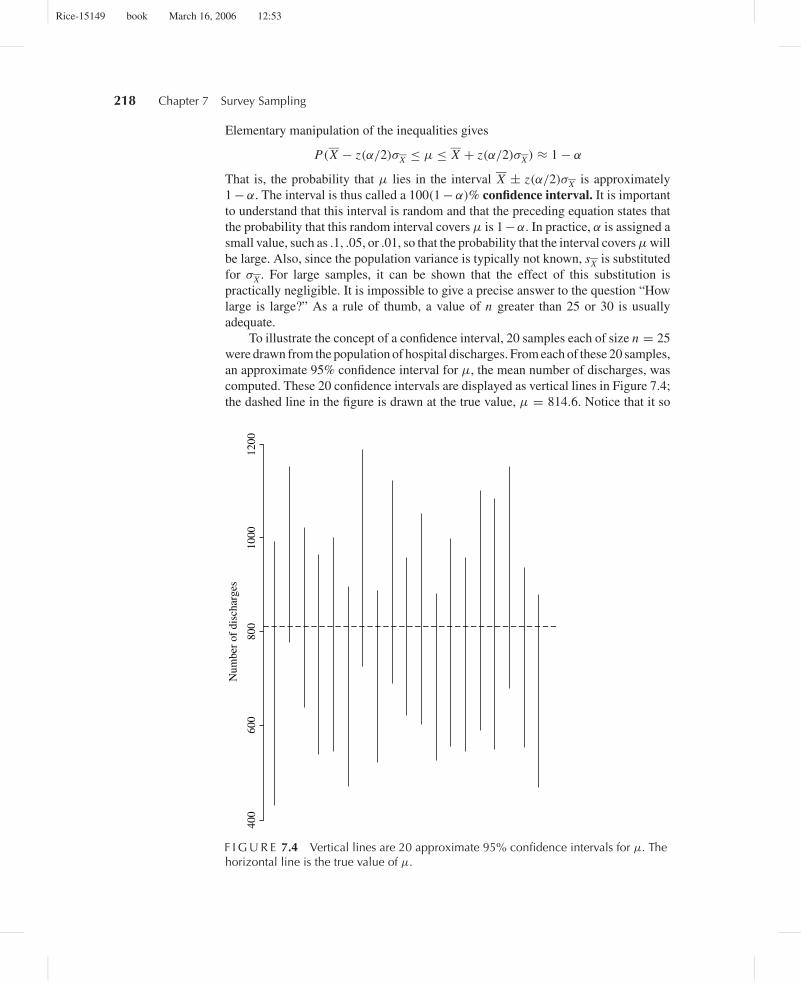
To illustrate the concept of a confidence interval, 20 samples each of size n = 25were drawn from the population of hospital discharges. From each of these 20 samples,an approximate 95% confidence interval for µ, the mean number of discharges, wascomputed. These 20 confidence intervals are displayed as vertical lines in Figure 7.4;the dashed line in the figure is drawn at the true value, µ = 814.6. Notice that it so

400

600

800

Num

ber

of d

isch

arge

s

1000

1200

F I G U R E 7.4 Vertical lines are 20 approximate 95% confidence intervals for µ. Thehorizontal line is the true value of µ.

Rice-15149 book March 16, 2006 12:53


happened that all the confidence intervals included µ; since these are 95% intervals,on the average 5%, or 1 out of 20, would not include µ.

The following example illustrates the procedure for calculating confidenceintervals.

E X A M P L E D A particular area contains 8000 condominium units. In a survey of the occupants, asimple random sample of size 100 yields the information that the average number ofmotor vehicles per unit is 1.6, with a sample standard deviation of .8. The estimatedstandard error of X is thus

sX = s√n

√1 − n

N

= .8

10

√1 − 100

8000= .08

Note that the finite population correction makes almost no difference. Since z(.025) =1.96, a 95% confidence interval for the population average is X ± 1.96sX , or (1.44,1.76).

An estimate of the total number of motor vehicles is T = 8000 × 1.6 = 12,800.

The estimated standard error of T is

sT = NsX = 640

A 95% confidence interval for the total number of motor vehicles is T ± 1.96sT , or(11,546, 14,054).

In the same survey, 12% of the respondents said they planned to sell their condoswithin the next year; p = .12 is an estimate of the population proportion p. Theestimated standard error is

sp =√

p(1 − p)

n − 1

√1 − 100

8000= .03

A 95% confidence interval for p is p ± 1.96sp, or (.06, .18).The total number of owners planning to sell is estimated as T = N p = 960. The

estimated standard error of T is sT = Nsp = 240. A 95% confidence interval for thenumber in the population planning to sell is T ± 1.96sT , or (490, 1430). The properinterpretation of this interval, (490, 1430), is a little subtle. We cannot state that theprobability is 0.95 and that the number of owners planning to sell is between 490 and1430, because that number is either in this interval or not. What is true is that 95% ofintervals formed in this way will contain the true number in the long run. This intervalis like one of those shown in Figure 7.4; in the long run, 95% of those intervals willcontain the true number of discharges, but in the figure any particular interval eitherdoes or doesn’t contain the true number. ■

The width of a confidence interval is determined by the sample size n and thepopulation standard deviation σ . If σ is known approximately, perhaps from earlier

Rice-15149 book March 16, 2006 12:53


samples of the population, n can be chosen so as to obtain a confidence interval closeto some desired length. Such analysis is usually an important aspect of planning thedesign of a sample survey.

E X A M P L E E The interval for the total number of owners planning to sell in Example D might beconsidered too wide for practical purposes; reducing its width would require a largersample size. Suppose that an interval with a half-width of 200 is desired. Neglectingthe finite population correction, the half-width is

1.96sT = 1.96N

√p(1 − p)

n − 1= 5095√

n − 1

Setting the last expression equal to 200 and solving for n yields n = 650 as thenecessary sample size. ■

Let us summarize: The fundamental result of this section is that the samplingdistribution of the sample mean is approximately Gaussian. This approximation can beused to quantify the error committed in estimating the population mean by the samplemean, thus giving us a good understanding of the accuracy of estimates producedby a simple random sample. We next introduced the idea of a confidence interval,a random interval that contains a population parameter with a specified probabilityand thus provides an assessment of the accuracy of the corresponding estimate of thatparameter. We have seen in our examples that the width of the confidence interval is amultiple of the estimated standard deviation of the estimate; for example, a confidenceinterval for µ is X ± ksX , where the constant k depends on the coverage probabilityof the interval.

7.4 Estimation of a RatioThe foundations of the theory of survey sampling have been laid in the preceding sec-tions on simple random sampling. This and the next section build on that foundation,developing some advanced topics in survey sampling.

In this section, we consider the estimation of a ratio. Suppose that for each memberof a population, two values, x and y, may be measured. The ratio of interest is

r =

N∑i=1

yi

N∑i=1

xi

= µy

µx

Ratios arise frequently in sample surveys; for example, if households are sampled,the following ratios might be calculated:

• If y is the number of unemployed males aged 20–30 in a household and x is thenumber of males aged 20–30 in a household, then r is the proportion of unemployedmales aged 20–30.

Rice-15149 book March 16, 2006 12:53

7.4 Estimation of a Ratio 221

• If y is weekly food expenditure and x is number of inhabitants, then r is weeklyfood cost per inhabitant.

• If y is the number of motor vehicles and x is the number of inhabitants of drivingage, then r is the number of motor vehicles per inhabitant of driving age.

In a survey of farms, y might be the acres of wheat planted and x the total acreage.In an inventory audit, y might be the audited value of an item and x the book value.

In this section, we first consider directly the problem of estimating a ratio. Later,we will use the estimation of a ratio as a technique for estimating µy . We will producea new estimate, the ratio estimate, which we will compare to the ordinary estimate, Y .

Before continuing, we note the elementary but sometimes overlooked fact that

r �= 1

N

N∑i=1

yi

xi

Suppose that a sample is drawn consisting of the pairs (Xi , Yi ); the naturalestimate of r is R = Y/X . We wish to derive expressions for E(R) and Var(R), butsince R is a nonlinear function of the random variables X and Y , we cannot do thisin closed form. We will therefore employ the approximate methods of Section 4.6.

In order to calculate the approximate variance of R, we need to know Var(X),Var(Y ), and Cov(X , Y ). The first two quantities we know from Theorem B of Section7.3.1. For the last quantity, we define the population covariance of x and y to be

σxy = 1

N

N∑i=1

(xi − µx)( yi − µy)

It can then be shown, in a manner entirely analogous to the proof of Theorem B inSection 7.3.1, that

Cov(X , Y ) = σxy

n

(1 − n − 1

N − 1

)From Example C in Section 4.6, we have the following theorem.

T H E O R E M A

With simple random sampling, the approximate variance of R = Y/X is

Var(R) ≈ 1

µ2x

(r 2σ 2

X+ σ 2

Y− 2rσXY

)

= 1

n

(1 − n − 1

N − 1

)1

µ2x

(r 2σ 2

x + σ 2y − 2rσxy

)■

The population correlation coefficient is defined as

ρ = σxy

σxσy

and is used as a measure of the strength of the linear relationship between the x andy values in the population. It can be shown that −1 ≤ ρ ≤ 1; large values of ρ

Rice-15149 book March 16, 2006 12:53


indicate a strong positive relationship between x and y, and small values indicate astrong negative relationship. (See Figure 4.7 for some illustrations of correlation.)The equation in Theorem A can be expressed in terms of the population correlationcoefficient as follows:

Var(R) ≈ 1

n

(1 − n − 1

N − 1

)1

µ2x

(r 2σ 2

x + σ 2y − 2rρσxσy

)From this expression, we see that strong correlation of the same sign as r decreases thevariance. We also note that the variance is affected by the size of µx —if µx is small,the variance is large, essentially because small values of X in the ratio R = Y/Xcause R to fluctuate wildly.

We now consider the approximate expectation of R. From Example C in Section4.6 and the preceding calculations, we have the following theorem.

T H E O R E M B

With simple random sampling, the expectation of R is given approximately by

E(R) ≈ r + 1

n

(1 − n − 1

N − 1

)1

µ2x

(rσ 2

x − ρσxσy

)■

From the equation in Theorem B, we see that strong correlation of the samesign as r decreases the bias and that the bias is large if µx is small. Furthermore,note that the bias is of the order 1/n, so its contribution to the mean squared error isof the order 1/n2. In comparison, the contribution of the variance is of the order 1/n.Therefore, for large samples, the bias is negligible compared to the standard error ofthe estimate.

For large samples, truncating the Taylor series after the linear term provides agood approximation, since the deviations X − µX and Y − µY are likely to be small.To this order of approximation, R is expressed as a linear combination of X and Y ,and an argument based on the central limit theorem can be used to show that R isapproximately normally distributed. Approximate confidence intervals can thus beformed for r by using the normal distribution.

In order to estimate the standard error of R, we substitute R for r in the formulaof Theorem A. The x and y population variances are estimated by s2

x and s2y . The

population covariance is estimated by

sxy = 1

n − 1

n∑i=1

(Xi − X)(Yi − Y )

= 1

n − 1

(n∑

i=1

Xi Yi − nXY

)

(as can be seen by expanding the product), and the population correlation is estimatedby

ρ = sxy

sx sy

Rice-15149 book March 16, 2006 12:53


The estimated variance of R is thus

s2R = 1

n

(1 − n − 1

N − 1

)1

X2 (R2s2

x + s2y − 2Rsxy)

An approximate 100(1 − α)% confidence interval for r is R ± z(α/2)sR .

E X A M P L E A Suppose that 100 people who recently bought houses are surveyed, and the monthlymortgage payment and gross income of each buyer are determined. Let y denote themortgage payment and x the gross income. Suppose that

X = $3100 Y = $868

sy = $250 sx = $1200

ρ = .85 R = .28

Neglecting the finite population correction, the estimated standard error of R is

sR = 1

10

(1

3100

) √.282 × 12002 + 2502 − 2 × .28 × .85 × 250 × 1200

= .006

An approximate 95% confidence interval for r is .28 ±(1.96)× (.006), or .28± .012.Note that the high correlation between x and y causes the standard error of R to besmall. We can use the observed values for the variances, covariances, and means togauge the order of magnitude of the bias by substituting them in place of the populationparameters in the formula of Theorem B. Doing so, and again neglecting the finitepopulation correction, gives the value .00015 for the bias, which is negligible relativeto sR . Note that the large value of X and the large positive correlation coefficientcause the bias to be small. ■

Ratios may also be used as tools for estimating population means and totals.To illustrate the concept, we return to the example of hospital discharges. For thispopulation, the number of beds in each hospital is also known; let us denote the numberof beds in the i th hospital by xi and the number of discharges by yi . Suppose thatall the xi are known, perhaps from an earlier enumeration, before a sample has beentaken to estimate the number of discharges, and that we would like to take advantageof this information. One way to do this is to form a ratio estimate of µy :

Y R = µx

XY = µx R

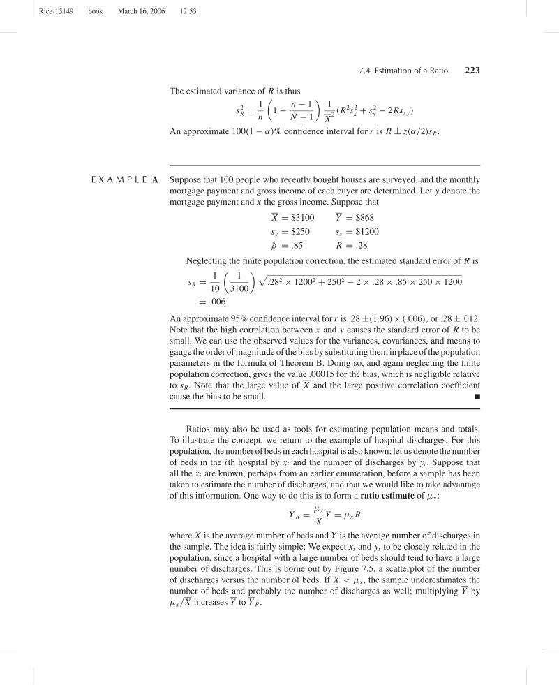
where X is the average number of beds and Y is the average number of discharges inthe sample. The idea is fairly simple: We expect xi and yi to be closely related in thepopulation, since a hospital with a large number of beds should tend to have a largenumber of discharges. This is borne out by Figure 7.5, a scatterplot of the numberof discharges versus the number of beds. If X < µx , the sample underestimates thenumber of beds and probably the number of discharges as well; multiplying Y byµx/X increases Y to Y R .

Rice-15149 book March 16, 2006 12:53


0

500

200 400 600 800

Dis

char

ges

Beds

1000

0 1000

1500

2000

2500

3000

F I G U R E 7.5 Scatterplot of the number of discharges versus the number of beds forthe 393 hospitals.

0600 700 800

Mean of simple random sample900

Cou

nt

40

80

500 1000

(a)

1100

120

0600 700 800

Ratio estimate

900

Cou

nt

40

80

500 1000

(b)

1100

120

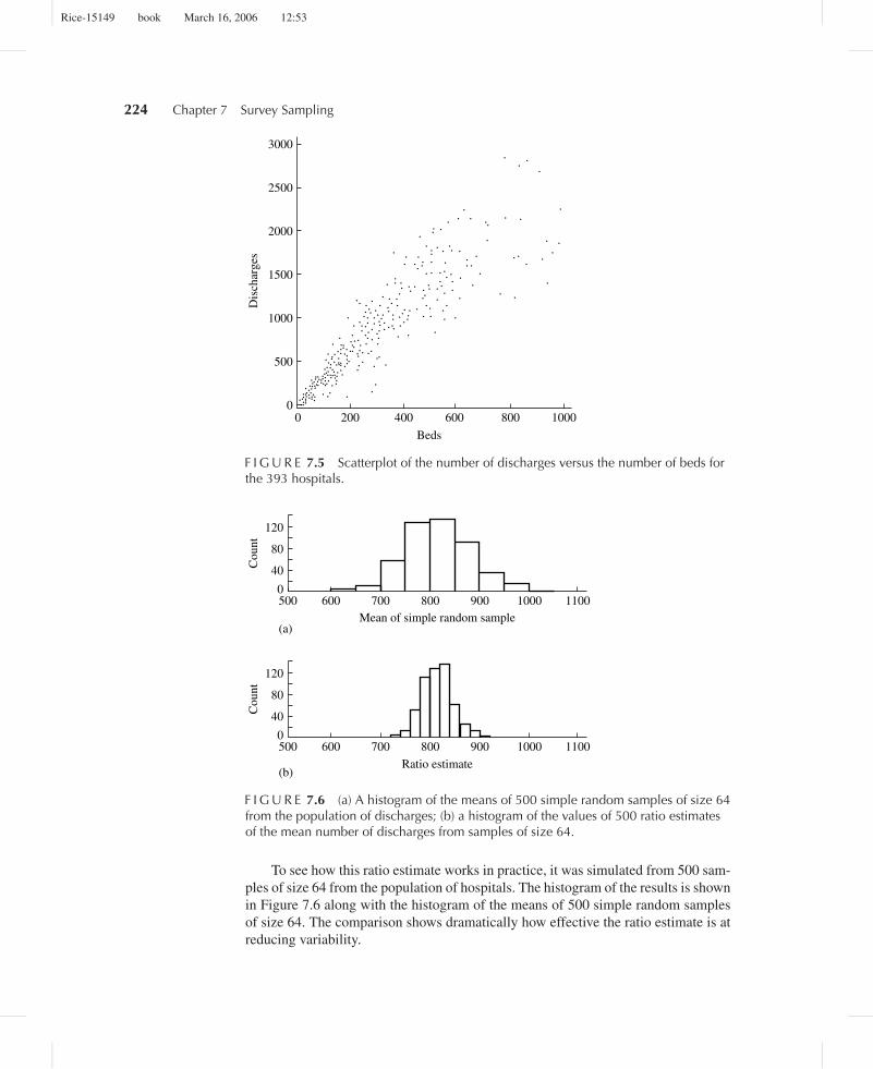
F I G U R E 7.6 (a) A histogram of the means of 500 simple random samples of size 64from the population of discharges; (b) a histogram of the values of 500 ratio estimatesof the mean number of discharges from samples of size 64.

To see how this ratio estimate works in practice, it was simulated from 500 sam-ples of size 64 from the population of hospitals. The histogram of the results is shownin Figure 7.6 along with the histogram of the means of 500 simple random samplesof size 64. The comparison shows dramatically how effective the ratio estimate is atreducing variability.

Rice-15149 book March 16, 2006 12:53


Two more examples will illustrate the scope of the ratio estimation method.

E X A M P L E B Suppose that we want to estimate the total number of unemployed males aged 20–30from a sample of households and that we know τx , the total number of males aged20–30, from census data. The ratio estimate is

TR = τxY

X

where Y is the average number of unemployed males aged 20–30 per household inthe sample, and X is the sample average number of males aged 20–30 per house-hold. ■

E X A M P L E C A sample of items in an inventory is taken to estimate the total value of the inventory.Let Yi be the audited value of the i th sample item, and let Xi be its book value. Weassume that τx , the total book value of the inventory, is known, and we estimate thetotal audited value by

TR = τxY

X■

We will now analyze the observed success of the ratio estimate. Since Y R = µX R,

Var(Y R) = µ2X Var(R). From Theorem A, we thus have the following.

C O R O L L A R Y A

The approximate variance of the ratio estimate of µy is

Var(Y R) ≈ 1

n

(1 − n − 1

N − 1

) (r 2σ 2

x + σ 2y − 2rρσxσy

)■

Similarly, from Theorem B, we have another corollary.

C O R O L L A R Y B

The approximate bias of the ratio estimate of µy is

E(Y R) − µY ≈ 1

n

(1 − n − 1

N − 1

)1

µx

(rσ 2

x − ρσxσy

)■

When will the ratio estimate YR be better than the ordinary estimate Y ? In the fol-lowing, the finite population correction is neglected for simplicity. Since the varianceof the ordinary estimate Y is

Var(Y ) = σ 2y

n

Rice-15149 book March 16, 2006 12:53


the ratio estimate has a smaller variance if

r 2σ 2x − 2rρσxσy < 0

or (provided r > 0, for example)

2ρσy > rσx

Letting Cx = σx/µx and Cy = σy/µy , this last inequality is equivalent to

ρ >1

2

(Cx

Cy

)Cx and Cy are called coefficients of variation and give the standard deviation as aproportion of the mean. (Coefficients of variation are often more meaningful thanstandard deviations. For example, a standard deviation of 10 means one thing if thetrue value of the quantity being measured is 100 and something entirely different ifthe true value is 10,000.)

In order to assess the accuracy of Y R , Var(Y R) can be estimated from the sample.

C O R O L L A R Y C

The variance of Y R can be estimated by

s2Y R

= 1

n

(1 − n − 1

N − 1

) (R2s2

x + s2y − 2Rsxy

)and an approximate 100(1 − α)% confidence interval for µy is (Y R ±z( α

2 )sY R). ■

E X A M P L E D For the population of 393 hospitals, we have

µx = 274.8 σx = 213.2µy = 814.6 σy = 589.7r = 2.96 ρ = .91

Thus,

Var(Y R) ≈ 1

n(2.962 × 213.22 + 589.72 − 2 × 2.96 × .91 × 213.2 × 589.7)

= 68,697.4

nand

σY R≈ 262.1√

n

Including the finite population correction, the linearized approximation predicts that,with n = 64,

σY R= 1

8(262.1)

√1 − 63

392= 30.0

Rice-15149 book March 16, 2006 12:53

7.5 Stratified Random Sampling 227

The actual standard deviation of the 500 sample values displayed in Figure 7.6 is29.9, which is remarkably close. The mean of the 500 values is 816.2, compared tothe population mean of 814.6; the slight apparent bias is consistent with Corollary B.

In contrast, the standard deviation of Y from a simple random sample of sizen = 64 is

σY = σ√n

√1 − n − 1

N − 1

= 589.7

8

√1 − 63

329= 66.3

The comparison of σY to σY Ris consistent with the substantial reduction in variability

accomplished by using a ratio estimate of µy shown in Figure 7.6.The following is another way of interpreting this comparison. If a simple random

sample of size n1 is taken, the variance of the estimate is Var(Y ) = 589.72/n1. Aratio estimate from a sample of size n2 will have the same variance if

262.12

n2= 589.72

n1

or

n2 = n1

(262.1

589.7

)2

= .1975n1

Thus, in this case, we can obtain the same precision from a ratio estimate using asample about 80% smaller than the simple random sample. Note that this comparisonneglects the bias of the ratio estimate, which is justifiable in this case because the biasis quite small. Here is a case in which a biased estimate performs substantially betterthan an unbiased estimate, the bias being quite small and the reduction in variancebeing quite large. ■

7.5 Stratified Random Sampling

7.5.1 Introduction and NotationIn stratified random sampling, the population is partitioned into subpopulations, orstrata, which are then independently sampled. The results from the strata are thencombined to estimate population parameters, such as the mean.

Following are some examples that suggest the range of situations in which strat-ification is natural:

• In auditing financial transactions, the transactions may be grouped into strata onthe basis of their nominal values. For example, high-value, medium-value, andlow-value strata might be formed.

• In samples of human populations, geographical areas often form natural strata.• In a study of records of shipments of household goods by motor carriers, the carriers

were grouped into three strata: large carriers, medium carriers, and small carriers.

John Rice

Note

63/392

Rice-15149 book March 16, 2006 12:53


Stratified samples are used for a variety of reasons. We are often interested inobtaining information about each of a number of natural subpopulations in additionto information about the population as a whole. The subpopulations might be definedby geographical areas or age groups. In an industrial application in which the popula-tion consists of items produced by a manufacturing process, relevant subpopulationsmight consist of items produced during different shifts or from different lots of rawmaterial. The use of a stratified random sample guarantees a prescribed number ofobservations from each subpopulation, whereas the use of a simple random samplecan result in underrepresentation of some subpopulations. A second reason for usingstratification is that, as will be shown below, the stratified sample mean can be con-siderably more precise than the mean of a simple random sample, especially if thepopulation members within each stratum are relatively homogeneous and if there isconsiderable variation between strata.

In the next section, properties of the stratified sample mean are derived. Sincea simple random sample is taken within each stratum, the results will follow easilyfrom the derivations of earlier sections. The section after that takes up the problemof how to allocate the total number of observations, n, among the various strata.Comparisons will be made of the efficiencies of different allocation schemes andalso of the precisions of these allocation schemes relative to that of a simple randomsample of the same total size.

7.5.2 Properties of Stratified EstimatesSuppose there are L strata in all. Let the number of population elements in stratum1 be denoted by N1, the number in stratum 2 be N2, etc. The total population sizeis N = N1 + N2 + . . . + NL . The population mean and variance of the lth stratumare denoted by µl and σ 2

l . The overall population mean can be expressed in terms ofthe µl as follows. Let xil denote the i th population value in the lth stratum and letWl = Nl/N denote the fraction of the population in the lth stratum. Then

µ = 1

N

L∑l=1

Nl∑i=1

xil

= 1

N

L∑l=1

Nlµl

=L∑

l=1

Wlµl

Within each stratum, a simple random sample of size nl is taken. The samplemean in stratum l is denoted by

Xl = 1

nl

nl∑i=1

Xil

Here Xil denotes the i th sample value in the lth stratum. Note that Xl is the mean ofa simple random sample from the population consisting of the lth stratum, so fromTheorem A of Section 7.3.1, E(Xl) = µl . By analogy with the preceding relationship

Rice-15149 book March 16, 2006 12:53


between the overall population mean and the population means of the various strata,the obvious estimate of µ is

Xs =L∑

l=1

Nl Xl

N

=L∑

l=1

Wl Xl

T H E O R E M A

The stratified estimate, Xs , of the population mean is unbiased.

Proof

E(Xs) =L∑

l=1

Wl E(Xl)

= 1

N

L∑l=1

Nlµl

= µ ■

Since we assume that the samples from different strata are independent of oneanother and that within each stratum a simple random sample is taken, the varianceof Xs can be easily calculated.

T H E O R E M B

The variance of the stratified sample mean is given by

Var(Xs) =L∑

l=1

W 2l

(1

nl

) (1 − nl − 1

Nl − 1

)σ 2

l

Proof

Since the Xl are independent,

Var(Xs) =L∑

l=1

W 2l Var(Xl)

From Theorem B of Section 7.3.1, we have

Var(Xl) = 1

nl

(1 − nl − 1

Nl − 1

)σ 2

l

Therefore, the desired result follows. ■

Rice-15149 book March 16, 2006 12:53


If the sampling fractions within all strata are small,

Var(Xs) ≈L∑

l=1

W 2l σ 2

l

nl

E X A M P L E A We again consider the population of hospitals. As we did in the discussion of ratioestimates, we assume that the number of beds in each hospital is known but that thenumber of discharges is not. We will try to make use of this knowledge by stratifyingthe hospitals according to the number of beds. Let stratum A consist of the 98 smallesthospitals, stratum B of the 98 next larger, stratum C of the 98 next larger, and stratumD of the 99 largest. The following table shows the results of this stratification ofhospitals by size:

Stratum Nl Wl µl σl

A 98 .249 182.9 103.4B 98 .249 526.5 204.8C 98 .249 956.3 243.5D 99 .251 1591.2 419.2

Suppose that we use a sample of total size n and let

n1 = n2 = n3 = n4 = n

4so that we have equal sample sizes in each stratum. Then, from Theorem B, neglectingthe finite population corrections and using the numerical values in the preceding table,we have

Var(Xs) =4∑

l=1

W 2l σ 2

l

n1

= 4

n

4∑l=1

W 2l σ 2

l

= 72, 042.6

nand

σXs= 268.4√

n

The standard deviation of the mean of a simple random sample is

σX = 587.7√n

Comparing the two standard deviations, we see that a tremendous gain in precisionhas resulted from the stratification. The ratio of the variances is .20; thus a stratifiedestimate based on a total sample size of n/5 is as precise as a simple random sampleof size n. The reduction in variance due to stratification is comparable to that achieved

Rice-15149 book March 16, 2006 12:53


by using a ratio estimate (Example D in Section 7.4). In later parts of this section, wewill look more analytically at why the stratification done here produced such dramaticimprovement. ■

Let us next consider the stratified estimate of the population total, Ts = N Xs .From Theorem B, we have the following corollary.

C O R O L L A R Y A

The expectation and variance of the stratified estimate of the population total are

E(Ts) = τ

and

Var(Ts) = N 2Var(Xs)

=L∑

l=1

N 2l

(1

nl

) (1 − nl − 1

Nl − 1

)σ 2

l ■

In order to estimate the standard errors of Xs and Ts , the variances of the individualstrata must be separately estimated and substituted into the preceding formulae. Theestimate of σ 2

l is given by

s2l = 1

nl − 1

nl∑i=1

(Xil − Xl)2

Var(Xs) is estimated by

s2Xs

=L∑

l=1

W 2l

(1

nl

) (1 − nl

Nl

)s2

l

The next example illustrates how this variance estimate can be used to findapproximate confidence intervals for µ based on Xs .

E X A M P L E B A sample of size 10 was drawn from each of the four strata of hospitals described inExample A, yielding the following:

X 1 = 240.6 s21 = 6827.6

X 2 = 507.4 s22 = 23,790.7

X 3 = 865.1 s23 = 42,573.0

X 4 = 1716.5 s24 = 152,099.6

Rice-15149 book March 16, 2006 12:53


Therefore, Xs = 832.5. The variance of the stratified sample mean is estimated by

s2Xs

= 1

10

4∑l=1

W 2l

(1 − nl − 1

Nl − 1

)s2

l

= 1282.0

Thus,

sXs= 35.8

An approximate 95% confidence interval for the population mean number of dis-charges is Xs ± 1.96sxs , or (762.4, 902.7).

The total number of discharges is estimated by Ts = 393Xs = 327,172. Thestandard error of Ts is estimated by sTs = 393sXs

= 14,069. An approximate95% confidence interval for the population total is Ts ± 1.96sTs , or (299,596, 354,748). ■

7.5.3 Methods of AllocationIn Section 7.5.2, it was shown that, neglecting the finite population correction,

Var(Xs) =L∑

l=1

W 2l σ 2

l

nl

If the resources of a survey allow only a total of n units to be sampled, the questionarises of how to choose n1, . . . , nL to minimize Var(Xs) subject to the constraintn1 + · · · + nL = n.

For the sake of simplicity, the calculations in this section ignore the finite popu-lation correction within each stratum. The analysis may be extended to include thesecorrections, but at the cost of some additional algebra. More complete results arecontained in Cochran (1977).

T H E O R E M A

The sample sizes n1, . . . , nL that minimize Var(Xs) subject to the constraintn1 + · · · + nL = n are given by

nl = nWlσl

L∑k=1

Wkσk

where l = 1, . . . , L .

Rice-15149 book March 16, 2006 12:53


Proof

We introduce a Lagrange multiplier, and we must then minimize

L(n1, . . . , nL , λ) =L∑

l=1

W 2l σ 2

l

nl+ λ

(L∑

l=1

nl − n

)

For l = 1, . . . , L , we have

∂L

∂nl= −W 2

l σ 2l

n2l

+ λ

Setting these partial derivatives equal to zero, we have the system of equations

nl = Wlσl√λ

for l = 1, . . . , L . To determine λ, we first sum these equations over l:

n = 1√λ

L∑l=1

Wlσl

Thus,1√λ

= nL∑

l=1Wlσl

andnl = n

Wlσl

L∑l=1

Wlσl

which proves the theorem. ■

This theorem shows that those strata for which Wlσl is large should be sampledheavily. This makes sense intuitively. If Wl is large, the stratum contains a largefraction of the population; if σl is large, the population values in the stratum arequite variable, and in order to obtain a good determination of the stratum’s mean, arelatively large sample size must be used. This optimal allocation scheme is calledNeyman allocation.

Substituting the optimal values of nl as given in Theorem A into the equation forVar(Xs) given in Theorem B in Section 7.5.2 gives us the following corollary.

C O R O L L A R Y A

Denoting by Xso, the stratified estimate using the optimal allocations as given inTheorem A and neglecting the finite population correction,

Var(Xso) =

(L∑

l=1Wlσl

)2

n■

Rice-15149 book March 16, 2006 12:53


E X A M P L E A For the population of hospitals, the weights for optimal allocation, Wlσl/∑

Wlσl ,are, from the table of Example A of Section 7.5.2,

Stratum

A B C DWeight .106 .210 .250 .434

Note that, because of its larger standard deviation, stratum D is sampled more thanfour times as heavily as stratum A. ■

The optimal allocations depend on the individual variances of the strata, whichgenerally will not be known. Furthermore, if a survey measures several attributesfor each population member, it is usually impossible to find an allocation that issimultaneously optimal for all of those variables. A simple and popular alternativemethod of allocation is to use the same sampling fraction in each stratum,

n1

N1= n2

N2= · · · = nL

NL

which holds if

nl = nNl

N= nWl

for l = 1, . . . , L . This method is called proportional allocation. The estimate of thepopulation mean based on proportional allocation is

Xsp =L∑

l=1

Wl Xl

=L∑

l=1

Wl1

nl

nl∑i=1

Xil

= 1

n

L∑l=1

nl∑i=1

Xil

since Wl/nl = 1/n. This estimate is simply the unweighted mean of the samplevalues.

T H E O R E M B

With stratified sampling based on proportional allocation, ignoring the finitepopulation correction,

Var(Xsp) = 1

n

L∑l=1

Wlσ2l

Rice-15149 book March 16, 2006 12:53


Proof

From Theorem B of Section 7.5.2, we have

Var(Xsp) =L∑

l=1

W 2l Var(Xl)

=L∑

l=1

W 2l

σ 2l

nl

Using nl = nWl , the result follows. ■

We now compare Var(Xsp) and Var(Xso) in order to discover the circumstancesunder which optimal allocation is substantially better than proportional allocation.

T H E O R E M C

With stratified random sampling, the difference between the variance of theestimate of the population mean based on proportional allocation and the varianceof that estimate based on optimal allocation is, ignoring the finite populationcorrection,

Var(Xsp) − Var(Xso) = 1

n

L∑l=1

Wl(σl − σ )2

where

σ =L∑

l=1

Wlσl

Proof

Var(Xsp) − Var(Xso) = 1

n

L∑

l=1

Wlσ2l −

(L∑

l=1

Wlσl

)2

The term within the large brackets equals∑L

l=1 Wl(σl − σ )2, which may beverified by expanding the square and collecting terms. ■

According to Theorem C, if the variances of the strata are all the same, propor-tional allocation yields the same results as optimal allocation. The more variable thesevariances are, the better it is to use optimal allocation.

Rice-15149 book March 16, 2006 12:53


E X A M P L E B Let us calculate how much better optimal allocation is than proportional allocationfor the population of hospitals. From Theorem C and Corollary A, we have

Var(Xsp) = Var(Xso) + 1

n

∑Wl(σl − σ )2

Therefore,

Var(Xsp)

Var(Xso)= 1 +

1

n

∑Wl(σl − σ )2

Var(Xso)

= 1 +∑

Wl(σl − σ )2

(∑

Wlσl)2

= 1 + .218

Thus, under proportional allocation, the variance of the mean is about 20% largerthan it is under optimal allocation. ■

We can also compare the variance under simple random sampling with the vari-ance under proportional allocation. The variance under simple random sampling is,neglecting the finite population correction,

Var(X) = σ 2

n

In order to compare this equation with that for the variance under proportional allo-cation, we need a relationship between the overall population variance, σ 2, and thestrata variances, σ 2

l . The overall population variance may be expressed as

σ 2 = 1

N

L∑l=1

Nl∑i=1

(xil − µ)2

Also,

(xil − µ)2 = [(xil − µl) + (µl − µ)]2

= (xil − µl)2 + 2(xil − µl)(µl − µ) + (µl − µ)2

When both sides of this last equation are summed over l, the middle term on theright-hand side becomes zero since Nlµl = ∑Nl

l=1 xil , so we have

Nl∑i=1

(xil − µ)2 =nl∑

i=1

(xil − µl)2 + Nl(µl − µ)2

= Nlσ2l + Nl(µl − µ)2

Dividing both sides by N and summing over l, we have

σ 2 =L∑

l=1

Wlσ2l +

L∑l=1

Wl(µl − µ)2

Rice-15149 book March 16, 2006 12:53


Substituting this expression for σ 2 into Var(X) = σ 2/n and using the formula forVar(Xsp) given in Theorem B completes a proof of the following theorem.

T H E O R E M D

The difference between the variance of the mean of a simple random sample andthe variance of the mean of a stratified random sample based on proportionalallocation is, neglecting the finite population correction,

Var(X) − Var(Xsp) = 1

n

L∑l=1

Wl(µl − µ)2■

Thus, stratified random sampling with proportional allocation always gives asmaller variance than does simple random sampling, providing that the finite popu-lation correction is ignored. Comparing the equations for the variances under simplerandom sampling, proportional allocation, and optimal allocation, we see that strat-ification with proportional allocation is better than simple random sampling if thestrata means are quite variable and that stratification with optimal allocation is evenbetter than stratification with proportional allocation if the strata standard deviationsare variable.

E X A M P L E C We calculate the improvement that would result from using stratification with propor-tional allocation rather than simple random sampling for the population of hospitals.From Theorems B and D, we have

Var(Xsrs)

Var(Xsp)= 1 +

∑Wl(µl − µ)2∑

Wlσ2l

= 1 + 3.83

As is frequently the case, the gain from using stratification with proportional allocationrather than simple random sampling is much greater than the gain from using optimalallocation rather than proportional allocation. Furthermore, proportional allocationrequires knowledge only of the sizes of the strata, whereas optimal allocation requiresknowledge of the standard deviations of the strata, and such knowledge is usuallyunavailable. ■

Typically, stratified random sampling can result in substantial increases in preci-sion for populations containing values that vary greatly in size. For example, a pop-ulation of transactions, a sample of which is to be audited for errors, might containtransactions in the hundreds of thousands of dollars and transactions in the hundredsof dollars. If such a population were divided into several strata according to the dollaramounts of the transactions, there might well be considerable variation in the meantransaction errors between the strata, since there may be rather large errors on large

Rice-15149 book March 16, 2006 12:53


transactions and small errors on small transactions. The variability of the errors mightalso be larger in the former strata as well.

We have not addressed the question of how many strata to form and how todefine the strata. In order to construct the optimal number of strata, the populationvalues themselves, which are of course unknown, would have to be used. Stratificationmust therefore be done on the basis of some related variable that is known (such astransaction amount in the preceding paragraph) or on the results of earlier samples.In practice, it usually turns out that such relationships are not strong enough to makeit worthwhile constructing more than a few strata.

7.6 Concluding RemarksThis chapter introduced survey sampling. It first covered the most elementary methodof probability sampling—simple random sampling. The theory of this method under-lies the theory of more complex sampling techniques. Stratified sampling was also in-troduced and shown to increase the precision of estimates substantially in many cases.

Several concepts and techniques introduced here recur throughout statistics: theconcept of a random estimate of a population parameter, such as the population mean;bias; the standard error of an estimate; confidence intervals based on the central limittheorem; and linearization, or propagation of error.

The theory and technique of survey sampling go far beyond the material inthis introduction. One method that deserves mention because of its widespread useis systematic sampling. The population members are given in a list. If, say, a 10%sample is desired, every tenth member of the list is sampled starting from some randompoint among the first ten. If the list is in totally random order, this method is similarto simple random sampling. If, however, there is some correlation or relationshipbetween successive members, the method is more similar to stratified sampling. Theclear danger of this method is that there may be some periodic structure in the list, inwhich case bias can ensue.

Another commonly used method is cluster sampling. In sampling residentialhouseholds, a survey might choose blocks randomly and then either sample everydwelling on each chosen block or further subsample the dwellings. Because onewould expect dwellings within a single block to be relatively homogeneous, thismethod is typically less precise than a simple random sample of the same size.

We have developed a mathematical model for survey sampling and have deducedconsequences of that model, including probabilistic error bounds for the estimates.As is always the case, reality never quite matches the mathematical model. Thebasic assumptions of the model are (1) that every population member appears inthe sample with a specified probability and (2) that an exact measurement or responseis obtained from every sample member. In practice, neither assumption will hold pre-cisely. Converse and Traugott (1986) provide an interesting discussion of the practicaldifficulties of polls and surveys and consequences for the variability of the estimates.

The first assumption may fail because of the difficulty of obtaining an ex-act enumeration of the population or because of imprecision in its definition. Forexample, political surveys can be putatively based on all adults, all registered voters,or all “likely” voters. However, the most serious problem with respect to the first

Rice-15149 book March 16, 2006 12:53

7.7 Problems 239

assumption is that of nonresponse. Response levels of only 60% to 70% are commonin surveys of human populations. The possibility of substantial bias clearly arises ifthere is a relationship of potential answers to survey questions to the propensity torespond to those questions. For example, adults living in families are easier to contactby a telephone survey than those living alone, and the opinions of these two groupsmay well differ on certain issues. It is important to realize that the standard errorsof estimates that we have developed earlier in this chapter account only for randomvariability in sample composition, not for systematic biases.

The Literary Digest poll of 1936, which predicted a 57% to 43% victory forRepublican Alfred Landon over incumbent president Franklin Roosevelt, is one ofthe most famous of flawed surveys. Questionnaires were mailed to about 10 millionvoters, who were selected from lists such as telephone books and club memberships,and approximately 2.4 million of the questionnaires were returned. There were twointrinsic problems: (1) nonresponse—those who did not respond may have voted dif-ferently from those who did—and (2) selection bias—even if all 10 million votershad responded, they would not have constituted a random sample; those in lowersocioeconomic classes (who were more likely to vote for Roosevelt) were less likelyto have telephone service or belong to clubs and thus less likely to be included inthe sample than were wealthier voters. The assumption that an exact measurement isobtained from every member of the sample may also be in error. In surveys conductedby interviewers, the interviewer’s approach and personality may affect the response.In surveys that use questionnaires, the wording of the questions and the context withinwhich they are lodged can have an effect. An interesting example is a poll conductedby Stanley Presser, (New Yorker, Oct 18, 2004). Half of the sample was asked, “Doyou think the United States should allow public speeches against democracy?” Theother half was asked, “Do you think the United States should forbid public speechesagainst democracy?” 56% said no to the first question, and 39% said yes to the second.The interesting paper by Hansen in Tanur et al. (1972) reports on efforts of the U.S.Bureau of the Census to investigate these sorts of problems.

7.7 Problems1. Consider a population consisting of five values—1, 2, 2, 4, and 8. Find the

population mean and variance. Calculate the sampling distribution of the meanof a sample of size 2 by generating all possible such samples. From them, findthe mean and variance of the sampling distribution, and compare the results toTheorems A and B in Section 7.3.1.

2. Suppose that a sample of size n = 2 is drawn from the population of the precedingproblem and that the proportion of the sample values that are greater than 3 isrecorded. Find the sampling distribution of this statistic by listing all possiblesuch samples. Find the mean and variance of the sampling distribution.

3. Which of the following is a random variable?

a. The population meanb. The population size, N

Rice-15149 book March 16, 2006 12:53


c. The sample size, nd. The sample meane. The variance of the sample meanf. The largest value in the sampleg. The population varianceh. The estimated variance of the sample mean

4. Two populations are surveyed with simple random samples. A sample of size n1

is used for population I, which has a population standard deviation σ1; a sample ofsize n2 = 2n1 is used for population II, which has a population standard deviationσ2 = 2σ1. Ignoring finite population corrections, in which of the two sampleswould you expect the estimate of the population mean to be more accurate?

5. How would you respond to a friend who asks you, “How can we say that thesample mean is a random variable when it is just a number, like the populationmean? For example, in Example A of Section 7.3.2, a simple random sam-ple of size 50 produced x = 938.5; how can the number 938.5 be a randomvariable?”

6. Suppose that two populations have equal population variances but are of differentsizes: N1 = 100,000 and N2 = 10,000,000. Compare the variances of the samplemeans for a sample of size n = 25. Is it substantially easier to estimate the meanof the smaller population?

7. Suppose that a simple random sample is used to estimate the proportion of familiesin a certain area that are living below the poverty level. If this proportion is roughly.15, what sample size is necessary so that the standard error of the estimate is .02?

8. A sample of size n = 100 is taken from a population that has a proportionp = 1/5.

a. Find δ such that P(| p − p| ≥ δ) = 0.025.b. If, in the sample, p = 0.25, will the 95% confidence interval for p contain

the true value of p?

9. In a simple random sample of 1,500 voters, 55% said they planned to vote for aparticular proposition, and 45% said they planned to vote against it. The estimatedmargin of victory for the proposition is thus 10%. What is the standard error ofthis estimated margin? What is an approximate 95% confidence interval for themargin?

10. True or false (and state why):If a sample from a population is large, a histogram of the values in the samplewill be approximately normal, even if the population is not normal.

11. Consider a population of size four, the members of which have values x1, x2, x3, x4.

a. If simple random sampling were used, how many samples of size two arethere?

b. Suppose that rather than simple random sampling, the following samplingscheme is used. The possible samples of size two are

{x1, x2}, {x2, x3}, {x3, x4}, {x1, x4}

Rice-15149 book March 16, 2006 12:53

7.7 Problems 241

and the sampling is done in such a way that each of these four possible samplesis equally likely. Is the sample mean unbiased?

12. Consider simple random sampling with replacement.

a. Show that

s2 = 1

n − 1

n∑i=1

(Xi − X)2

is an unbiased estimate of σ 2.b. Is s an unbiased estimate of σ?c. Show that n−1s2 is an unbiased estimate of σ 2

X.

d. Show that n−1 N 2s2 is an unbiased estimate of σ 2T .

e. Show that p(1 − p)/(n − 1) is an unbiased estimate of σ 2p .

13. Suppose that the total number of discharges, τ , in Example A of Section 7.2 isestimated from a simple random sample of size 50. Denoting the estimate by T ,use the central limit theorem to sketch the approximate probability density of theerror T − τ .

14. The proportion of hospitals in Example A of Section 7.2 that had fewer than 1000discharges is p = .654. Suppose that the total number of hospitals having fewerthan 1000 discharges is estimated from a simple random sample of size 25. Usethe central limit theorem to sketch the approximate sampling distribution of theestimate.

15. Consider estimating the mean of the population of hospital discharges (Exam-ple A of Section 7.2) from a simple random sample of size n. Use the normalapproximation to the distribution of X in answering the following:

a. Sketch P(|X − µ| > 200) as a function of n for 20 ≤ n ≤ 100.b. For n = 20, 40, and 80, find � such that P(|X − µ| > �) ≈ .10. Similarly,

find � such that P(|X − µ| > �) ≈ .50.

16. True or false?

a. The center of a 95% confidence interval for the population mean is a randomvariable.

b. A 95% confidence interval for µ contains the sample mean with probability.95.

c. A 95% confidence interval contains 95% of the population.d. Out of one hundred 95% confidence intervals for µ, 95 will contain µ.

17. A 90% confidence interval for the average number of children per householdbased on a simple random sample is found to be (.7, 2.1). Can we conclude that90% of households have between .7 and 2.1 children?

18. From independent surveys of two populations, 90% confidence intervals for thepopulation means are constructed. What is the probability that neither intervalcontains the respective population mean? That both do?

19. This problem introduces the concept of a one-sided confidence interval. Usingthe central limit theorem, how should the constant k be chosen so that the interval

Rice-15149 book March 16, 2006 12:53


(−∞, X + ksX ) is a 90% confidence interval for µ—i.e., so that P(µ ≤ X +ksX ) = .9? This is called a one-sided confidence interval. How should k bechosen so that (X − ksX , ∞) is 95% one-sided confidence interval?

20. In Example D of Section 7.3.3, a 95% confidence interval for µ was found to be(1.44, 1.76). Because µ is some fixed number, it either lies in this interval or itdoesn’t, so it doesn’t make any sense to claim that P(1.44 ≤ µ ≤ 1.76) = .95.What do we mean, then, by saying this is a “95% confidence interval?”

21. In order to halve the width of a 95% confidence interval for a mean, by what factorshould the sample size be increased? Ignore the finite population correction.

22. An investigator quantifies her uncertainty about the estimate of a population meanby reporting X ± sX . What size confidence interval is this?

23. a. Show that the standard error of an estimated proportion is largest when p =1/2.

b. Use this result and Corollary B of Section 7.3.2 to conclude that thequantity

1

2

√N − n

N (n − 1)

is a conservative estimate of the standard error of p no matter what the valueof p may be.

c. Use the central limit theorem to conclude that the interval

p ±√

N − n

N (n − 1)

contains p with probability at least .95.

24. For a random sample of size n from a population of size N , consider the followingas an estimate of µ:

Xc =n∑

i=1

ci Xi

where the ci are fixed numbers and X1, . . . , Xn is the sample.

a. Find a condition on the ci such that the estimate is unbiased.b. Show that the choice of ci that minimizes the variances of the estimate subject

to this condition is ci = 1/n, where i = 1, . . . , n.

25. Here is an alternative proof of Lemma B in Section 7.3.1. Consider a randompermutation Y1, Y2, . . . , YN of x1, x2, . . . , xN . Argue that the joint distribution ofany subcollection, Yi1 , . . . , Yin , of the Yi is the same as that of a simple randomsample, X1, . . . , Xn. In particular,

Var(Yi ) = Var(Xk) = σ 2

and

Cov(Yi , Y j ) = Cov(Xk, Xl) = γ

Rice-15149 book March 16, 2006 12:53

7.7 Problems 243

if i �= j and k �= l. Since Y1 + Y2 + · · · + YN = τ ,

Var

(N∑

i=1

Yi

)= 0

(Why?) Express Var(∑N

i=1 Yi ) in terms of σ 2 and the unknown covariance, γ .Solve for γ , and conclude that

γ = − σ 2

N − 1for i �= j .

26. This is another proof of Lemma B in Section 7.3.1. Let Ui be a random vari-able with Ui = 1 if the i th population member is in the sample and equal to 0otherwise.

a. Show that the sample mean X = n−1∑N

i=1 Ui xi .b. Show that P(Ui = 1) = n/N . Find E(Ui ), using the fact that Ui is a Bernoulli

random variable.c. What is the variance of the Bernoulli random variable Ui ?d. Noting that UiU j is a Bernoulli random variable, find E(UiU j ), i �= j . (Be

careful to take into account that the sample is drawn without replacement.)e. Find Cov(Ui , U j ), i �= j .f. Using the representation of X above, find Var(X).

27. Suppose that the population size N is not known, but it is known that n ≤ N .Show that the following procedure will generate a simple random sample ofsize n. Imagine that the population is arranged in a long list that you can readsequentially.

a. Let the sample initially consist of the the first n elements in the list.b. For k = 1, 2, . . . , as long as the end of the list has not been encountered:

i. Read the (n + k)-th element in the list.ii. Place it in the sample with probability n/(n + k) and, if it is placed in the

sample, randomly drop one of the exisiting sample members.

28. In surveys, it is difficult to obtain accurate answers to sensitive questions such as“Have you ever used heroin?” or “Have you ever cheated on an exam?” Warner(1965) introduced the method of randomized response to deal with such sit-uations. A respondent spins an arrow on a wheel or draws a ball from an urncontaining balls of two colors to determine which of two statements to respondto: (1) “I have characteristic A,” or (2) “I do not have characteristic A.” The inter-viewer does not know which statement is being responded to but merely recordsa yes or a no. The hope is that an interviewee is more likely to answer truthfullyif he or she realizes that the interviewer does not know which statement is beingresponded to. Let R be the proportion of a sample answering Yes. Let p be theprobability that statement 1 is responded to (p is known from the structure ofthe randomizing device), and let q be the proportion of the population that hascharacteristic A. Let r be the probability that a respondent answers Yes.

a. Show that r = (2p−1)q+(1− p). [Hint: P(yes) = P(yes given question 1) ×P(question 1) + P(yes given question 2) × P(question 2).]

Rice-15149 book March 16, 2006 12:53


b. If r were known, how could q be determined?c. Show that E(R) = r , and propose an estimate, Q, for q. Show that the estimate

is unbiased.d. Ignoring the finite population correction, show that

Var(R) = r(1 − r)

n

where n is the sample size.e. Find an expression for Var(Q).

29. A variation of the method described in Problem 28 has been proposed. Insteadof responding to statement 2, the respondent answers an unrelated question forwhich the probability of a “yes” response is known, for example, “Were you bornin June?”

a. Propose an estimate of q for this method.b. Show that the estimate is unbiased.c. Obtain an expression for the variance of the estimate.

30. Compare the accuracies of the methods of Problems 28 and 29 by comparing theirstandard deviations. You may do this by substituting some plausible numericalvalues for p and q.

31. Referring to Example D in Section 7.3.3, how large should the sample be in orderthat the 95% confidence interval for the total number of owners planning to sellwill have a width of 500?

32. Referring again to Example D in Section 7.3.3, suppose that a survey is done ofanother condominium project of 12,000 units. The sample size is 200, and theproportion planning to sell in this sample is .18.

a. What is the standard error of this estimate? Give a 90% confidence interval.b. Suppose we use the notation p1 = .12 and p2 = .18 to refer to the proportions

in the two samples. Let d = p1 − p2 be an estimate of the difference, d, ofthe two population proportions p1 and p2. Using the fact that p1 and p2 areindependent random variables, find expressions for the variance and standarderror of d .

c. Because p1 and p2 are approximately normally distributed, so is d. Use thisfact to construct 99%, 95%, and 90% confidence intervals for d. Is there clearevidence that p1 is really different from p2?

33. Two populations are independently surveyed using simple random samples ofsize n, and two proportions, p1 and p2, are estimated. It is expected that bothpopulation proportions are close to .5. What should the sample size be so that thestandard error of the difference, p1 − p2, will be less than .02?

34. In a survey of a very large population, the incidences of two health problems areto be estimated from the same sample. It is expected that the first problem willaffect about 3% of the population and the second about 40%. Ignore the finitepopulation correction in answering the following questions.

Rice-15149 book March 16, 2006 12:53

7.7 Problems 245

a. How large should the sample be in order for the standard errors of both esti-mates to be less than .01? What are the actual standard errors for this samplesize?

b. Suppose that instead of imposing the same limit on both standard errors, theinvestigator wants the standard error to be less than 10% of the true value ineach case. What should the sample size be?

35. A simple random sample of a population of size 2000 yields the following25 values:

104 109 111 109 8786 80 119 88 12291 103 99 108 96

104 98 98 83 10779 87 94 92 97

a. Calculate an unbiased estimate of the population mean.b. Calculate unbiased estimates of the population variance and Var(X).c. Give approximate 95% confidence intervals for the population mean and total.

36. With simple random sampling, is X2

an unbiased estimate of µ2? If not, what isthe bias?

37. Two surveys were independently conducted to estimate a population mean, µ.Denote the estimates and their standard errors by X 1 and X 2 and σX1

and σX2.

Assume that X 1 and X 2 are unbiased. For some α and β, the two estimates canbe combined to give a better estimator:

X = αX 1 + β X 2

a. Find the conditions on α and β that make the combined estimate unbiased.b. What choice of α and β minimizes the variances, subject to the condition of

unbiasedness?

38. Let X1, . . . , Xn be a simple random sample. Show that1

n

n∑i=1

X 3i is an unbiased

estimate of1

N

N∑i=1

x3i .

39. Suppose that of a population of N items, k are defective in some way. For exam-ple, the items might be documents, a small proportion of which are fraudulent.How large should a sample be so that with a specified probability it will containat least one of the defective items? For example, if N = 10,000, k = 50, andp = .95, what should the sample size be? Such calculations are useful in planningsample sizes for acceptance sampling.

40. This problem presents an algorithm for drawing a simple random sample from apopulation in a sequential manner. The members of the population are consideredfor inclusion in the sample one at a time in some prespecified order (for example,the order in which they are listed). The i th member of the population is included

Rice-15149 book March 16, 2006 12:53


in the sample with probability

n − ni

N − i + 1

where ni is the number of population members already in the sample before thei th member is examined. Show that the sample selected in this way is in facta simple random sample; that is, show that every possible sample occurs withprobability

1(N

n

)

41. In accounting and auditing, the following sampling method is sometimes used toestimate a population total. In estimating the value of an inventory, suppose thata book value exists for each item and is readily accessible. For each item in thesample, the difference D, audited value minus book value, is determined. Theinventory value is estimated by the sum of the book values of the population andN D, where N is the population size.

a. Show that the estimate is unbiased.b. Find an expression for the variance of the estimate.c. Compare the expression obtained in part (b) to the variance of the usual es-

timate, which is the product of N and the average audited value. Under whatcircumstances would the proposed method be more accurate?

d. How could a ratio estimate be employed in this situation? Would there be anyadvantage or disadvantage to using a ratio estimate rather than the proposedmethod?

42. Show that the population correlation coefficient is less than or equal to 1 inabsolute value.

43. Suppose that for Example D in Section 7.3.3, the average number of occupantsper condominium unit in the sample is 2.2 with a sample standard deviation of.7 and the sample correlation coefficient between the number of occupants andthe number of motor vehicles is .85. Estimate the population ratio of the numberof motor vehicles per occupant and its standard error. Find an approximate 95%confidence interval for the estimate.

44. Show that

Var(Y R)

Var(Y )≈ 1 + Cx

Cy

(Cx

Cy− 2ρ

)

Sketch the graph of this ratio as a function of Cx/Cy .

45. In the population of hospitals, the correlation of the number of beds and the num-ber of discharges is ρ = .91 (Example D of Section 7.4). To see how Var(Y R)

would be different if the correlation were different, plot Var(Y R) for n = 64 asa function of ρ for −1 < ρ < 1.

Rice-15149 book March 16, 2006 12:53

7.7 Problems 247

46. Use the central limit theorem to sketch the approximate sampling distributionof Y R for n = 64 for the population of hospitals. Compare to the approximatesampling distribution of Y .

47. For the population of hospitals and a sample size of n = 64, find the approxi-mate bias of Y R by applying Corollary B of Section 7.4 and compare it to theapproximate standard deviation of the estimate. Repeat for n = 128.

48. A simple random sample of 100 households located in a city recorded the numberof people living in the household, X , and the weekly expenditure for food, Y . Itis known that there are 100,000 households in the city. In the sample∑

Xi = 320∑Yi = 10,000∑X 2

i = 1250∑Y 2

i = 1,100,000∑Xi Yi = 36,000

Neglect the finite population correction in answering the following.

a. Estimate the ratio r = µy/µx .b. Form an approximate 95% confidence interval for µy/µx .c. Using only the data on Y estimate the total weekly food expenditure, τ , for

households in the city and form a 90% confidence interval.

49. In a wildlife survey, an area of desert land was divided into 1000 squares, or“quadrats,” a simple random sample of 50 of which were surveyed. In each sur-veyed quadrat, the number of birds, Y , and the area covered by vegetation, X ,were determined. It was found that∑

Xi = 3000∑Yi = 150∑X 2

i = 225,000∑Y 2

i = 650∑Xi Yi = 11,000

a. Estimate the ratio of the average number of birds per quadrat to the averagevegetation cover per quadrat.

b. Estimate the standard error of your estimate and find an approximate 90%confidence interval for the population average.

c. Estimate the total number of birds and find an approximate 95% confidenceinterval for the population total.

d. Suppose that from an aerial survey, the total area covered by vegetation couldeasily be determined. How could this information be used to provide another

Rice-15149 book March 16, 2006 12:53


estimate of the number of birds? Would you expect this estimate to be betterthan or worse than that found in part (c)?

50. Hartley and Ross (1954) derived the following exact bound on the relative sizeof the bias and standard error of a ratio estimate:

|E(R) − r |σR

≤ σX

µx= σx

µx

√1

n

(1 − n − 1

N − 1

)

a. Derive this bound from the relation

Cov(R, X) = E

(Y

XX

)− E

(Y

X

)E(X)

b. Apply the bound to Problem 43 using sample estimates in place of the givenpopulation parameters.

51. This problem introduces a technique called the “jackknife,” originally proposedby Quenouille (1956) for reducing bias. Many nonlinear estimates, including theratio estimator, have the property that

E(θ) = θ + b1

n+ b2

n2+ · · ·

where θ is an estimate of θ . The jackknife forms an estimate θJ , which has aleading bias term of the order n−2 rather than n−1. Thus, for sufficiently largen, the bias of θJ is substantially smaller than that of θ . The technique involvessplitting the sample into several subsamples, computing the estimate for eachsubsample, and then combining the several estimates. The sample is split into pgroups of size m, where n = mp. For j = 1, . . . , p, the estimate θ j is calculatedfrom the m(p − 1) observations left after the j th group has been deleted. Fromthe preceding expression,

E(θ j ) = θ + b1

m(p − 1)+ b2

[m(p − 1)]2+ · · ·

Now, p “pseudovalues” are defined:

Vj = pθ − ( p − 1)θ j

The jackknife estimate, θJ , is defined as the average of the pseudovalues:

θJ = 1

p

p∑j=1

Vj

Show that the bias of θJ is of the order n−2.

52. A population consists of three strata with N1 = N2 = 1000 and N3 = 500.A stratified random sample with 10 observations in each stratum yields the

Rice-15149 book March 16, 2006 12:53

7.7 Problems 249

following data:

Stratum 1 94 99 106 106 101 102 122 104 97 97Stratum 2 183 183 179 211 178 179 192 192 201 177Stratum 3 343 302 286 317 289 284 357 288 314 276

Estimate the population mean and total and give a 90% confidence interval.

53. The following table (Cochran 1977) shows the stratification of all farms in acounty by farm size and the mean and standard deviation of the number of acresof corn in each stratum.

Farm Size Nl µl σl

0–40 394 5.4 8.341–80 461 16.3 13.381–120 391 24.3 15.1121–160 334 34.5 19.8161–200 169 42.1 24.5201–240 113 50.1 26.0241 + 148 63.8 35.2

a. For a sample size of 100 farms, compute the sample sizes from each stratumfor proportional and optimal allocation, and compare them.

b. Calculate the variances of the sample mean for each allocation and comparethem to each other and to the variance of an estimate formed from simplerandom sampling.

c. What are the population mean and variance?d. Suppose that ten farms are sampled per stratum. What is Var(Xs)? How large

a simple random sample would have to be taken to attain the same variance?Ignore the finite population correction.

e. Repeat part (d) using proportional allocation of the 70 samples.

54. a. Suppose that the cost of a survey is C = C0 + C1n, where C0 is a startupcost and C1 is the cost per observation. For a given cost C , find the al-location n1, . . . , nL to L strata that is optimal in the sense that it mini-mizes the variance of the estimate of the population mean subject to the costconstraint.

b. Suppose that the cost of an observation varies from stratum to stratum—insome strata the observations might be relatively cheap and in others relativelyexpensive. The cost of a survey with an allocation n1, . . . , nL is

C = C0 +L∑

l=1

Clnl

For a fixed total cost C , what choice of n1, · · ·, nL minimizes the variance?c. Assuming that the cost function is as given in part (b), for a fixed variance,

find nl to minimize cost.

Rice-15149 book March 16, 2006 12:53


55. The designer of a sample survey stratifies a population into two strata, H and L.H contains 100,000 people, and L contains 500,000. He decides to allocate 100samples to stratum H and 200 to stratum L, taking a simple random sample ineach stratum.

a. How should the designer estimate the population mean?b. Suppose that the population standard deviation in stratum H is 20 and the

standard deviation in stratum L is 10. What will be the standard error of hisestimate?

c. Would it be better to allocate 200 samples to stratum H and 100 to stratum L?d. Would it be better to use proportional allocation?

56. How might stratification be used in each of the following sampling problems?

a. A survey of household expenditures in a city.b. A survey to examine the lead concentration in the soil in a large plot of land.c. A survey to estimate the number of people who use elevators in a large building

with a single bank of elevators.d. A survey of programs on a television station, taken to estimate the proportion

of time taken up by advertising on Monday through Friday from 6 P.M. until10 P.M. Assume that 52 weeks of recorded broadcasts are available for analysis.

57. Consider stratifying the population of Problem 1 into two strata: (1, 2, 2) and (4,8). Assuming that one observation is taken from each stratum, find the samplingdistribution of the estimate of the population mean and the mean and standarddeviation of the sampling distribution. Compare to Theorems A and B in Section7.5.2 and the results of Problem 1.

58. (Computer Exercise) Construct a population consisting of the integers from 1 to100. Simulate the sampling distribution of the sample mean of a sample of size12 by drawing 100 samples of size 12 and making a histogram of the results.

59. (Computer Exercise) Continuing with Problem 58, divide the population intotwo strata of equal size, allocate six observations per stratum, and simulatethe distribution of the stratified estimate of the population mean. Do the samething with four strata. Compare the results to each other and to the results ofProblem 58.

60. A population consists of two strata, H and L , of sizes 100,000 and 500,000 andstandard deviations 20 and 12, respectively. A stratified sample of size 100 is tobe taken.

a. Find the optimal allocation for estimating the population mean.b. Find the optimal allocation for estimating the difference of the means of the

strata, µH − µL .

61. The value of a population mean increases linearly through time: µ(t) = α + βtwhile the variance remains constant. Independent simple random samples of sizen are taken at times t = 1, 2, and 3.

a. Find conditions on w1, w2, and w3 such that

β = w1 X 1 + w2 X 2 + w3 X 3

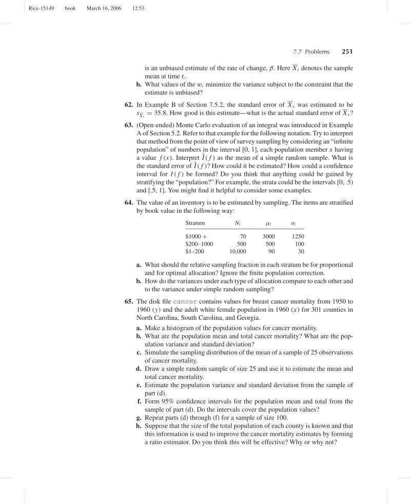
Rice-15149 book March 16, 2006 12:53

7.7 Problems 251

is an unbiased estimate of the rate of change, β. Here Xi denotes the samplemean at time ti .

b. What values of the wi minimize the variance subject to the constraint that theestimate is unbiased?

62. In Example B of Section 7.5.2, the standard error of Xs was estimated to besXs

= 35.8. How good is this estimate—what is the actual standard error of Xs?

63. (Open-ended) Monte Carlo evaluation of an integral was introduced in ExampleA of Section 5.2. Refer to that example for the following notation. Try to interpretthat method from the point of view of survey sampling by considering an “infinitepopulation” of numbers in the interval [0, 1], each population member x havinga value f (x). Interpret I ( f ) as the mean of a simple random sample. What isthe standard error of I ( f )? How could it be estimated? How could a confidenceinterval for I ( f ) be formed? Do you think that anything could be gained bystratifying the “population?” For example, the strata could be the intervals [0, .5)and [.5, 1]. You might find it helpful to consider some examples.

64. The value of an inventory is to be estimated by sampling. The items are stratifiedby book value in the following way:

Stratum Nl µl σl

$1000 + 70 3000 1250$200–1000 500 500 100$1–200 10,000 90 30

a. What should the relative sampling fraction in each stratum be for proportionaland for optimal allocation? Ignore the finite population correction.

b. How do the variances under each type of allocation compare to each other andto the variance under simple random sampling?

65. The disk file cancer contains values for breast cancer mortality from 1950 to1960 (y) and the adult white female population in 1960 (x) for 301 counties inNorth Carolina, South Carolina, and Georgia.

a. Make a histogram of the population values for cancer mortality.b. What are the population mean and total cancer mortality? What are the pop-

ulation variance and standard deviation?c. Simulate the sampling distribution of the mean of a sample of 25 observations

of cancer mortality.d. Draw a simple random sample of size 25 and use it to estimate the mean and

total cancer mortality.e. Estimate the population variance and standard deviation from the sample of

part (d).f. Form 95% confidence intervals for the population mean and total from the

sample of part (d). Do the intervals cover the population values?g. Repeat parts (d) through (f) for a sample of size 100.h. Suppose that the size of the total population of each county is known and that

this information is used to improve the cancer mortality estimates by forminga ratio estimator. Do you think this will be effective? Why or why not?

Rice-15149 book March 16, 2006 12:53


i. Simulate the sampling distribution of ratio estimators of mean cancer mortal-ity based on a simple random sample of size 25. Compare this result to thatof part (c).

j. Draw a simple random sample of size 25 and estimate the population mean andtotal cancer mortality by calculating ratio estimates. How do these estimatescompare to those formed in the usual way in part (d) from the same data?

k. Form confidence intervals about the estimates obtained in part ( j).l. Stratify the counties into four strata by population size. Randomly sample six

observations from each stratum and form estimates of the population meanand total mortality.

m. Stratify the counties into four strata by population size. What are the sam-pling fractions for proportional allocation and optimal allocation? Comparethe variances of the estimates of the population mean obtained using simplerandom sampling, proportional allocation, and optimal allocation.

n. How much better than those in part (m) will the estimates of the populationmean be if 8, 16, 32, or 64 strata are used instead?

66. A photograph of a large crowd on a beach is taken from a helicopter. The photois of such high resolution that when sections are magnified, individual peoplecan be identified, but to count the entire crowd in this way would be very time-consuming. Devise a plan to estimate the number of people on the beach by usinga sampling procedure.

67. The data set families contains information about 43,886 families living inthe city of Cyberville. The city has four regions: the Northern region has 10,149families, the Eastern region has 10,390 families, the Southern region has 13,457families, and the Western region has 9,890. For each family, the following infor-mation is recorded:

1. Family type1: Husband-wife family2: Male-head family3: Female-head family

2. Number of persons in family3. Number of children in family4. Family income5. Region

1: North2: East3: South4: West

6. Education level of head of household31: Less than 1st grade32: 1st, 2nd, 3rd, or 4th grade33: 5th or 6th grade34: 7th or 8th grade35: 9th grade36: 10th grade37: 11th grade

Rice-15149 book March 16, 2006 12:53

7.7 Problems 253

38: 12th grade, no diploma39: High school graduate, high school diploma, or equivalent40: Some college but no degree41: Associate degree in college (occupation/vocation program)42: Associate degree in college (academic program)43: Bachelor’s degree (e.g., B.S., B.A., A.B.)44: Master’s degree (e.g., M.S., M.A., M.B.A.)45: Professional school degree (e.g., M.D., D.D.S., D.V.M., LL.B., J.D.)46: Doctoral degree (e.g., Ph.D., Ed.D.)

In these exercises, you will try to learn about the families of Cyberville by usingsampling.

a. Take a simple random sample of 500 families. Estimate the following popula-tion parameters, calculate the estimated standard errors of these estimates, andform 95% confidence intervals:

i. The proportion of female-headed familiesii. The average number of children per family

iii. The proportion of heads of households who did not receive a high schooldiploma

iv. The average family income

Repeat the preceding parameters for five different simple random samples ofsize 500 and compare the results.

b. Take 100 samples of size 400.

i. For each sample, find the average family income.ii. Find the average and standard deviation of these 100 estimates and make

a histogram of the estimates.iii. Superimpose a plot of a normal density with that mean and standard devi-

ation of the histogram and comment on how well it appears to fit.iv. Plot the empirical cumulative distribution function (see Section 10.2). On

this plot, superimpose the normal cumulative distribution function withmean and standard deviation as earlier. Comment on the fit.

v. Another method for examining a normal approximation is via a normalprobability plot (Section 9.9). Make such a plot and comment on what itshows about the approximation.

vi. For each of the 100 samples, find a 95% confidence interval for the pop-ulation average income. How many of those intervals actually contain thepopulation target?

vii. Take 100 samples of size 100. Compare the averages, standard deviations,and histograms to those obtained for a sample of size 400 and explain howthe theory of simple random sampling relates to the comparisons.

c. For a simple random sample of 500, compare the incomes of the three familytypes by comparing histograms and boxplots (see Chapter 10.6).

d. Take simple random samples of size 400 from each of the four regions.

i. Compare the incomes by region by making parallel boxplots.ii. Does it appear that some regions have larger families than others?

iii. Are there differences in education level among the four regions?

Rice-15149 book March 16, 2006 12:53


e. Formulate a question of your choice and attempt to answer it with a simplerandom sample of size 400.

f. Does stratification help in estimating the average family income? From a simplerandom sample of size 400, estimate the average income and also the standarderror of your estimate. Form a 95% confidence interval. Next, allocate the 400observations proportionally to the four regions and estimate the average incomefrom the stratified sample. Estimate the standard error and form a 95% confi-dence interval. Compare your results to the results of the simple random sample.

Documents

Survey Sampling - Berkeleyrice/Book3ed/p227.pdf · Survey Sampling 7.1 Introduction ... for example, the U.S. government con- ... 7.3.1 The Expectation and Variance of the Sample