Embed Size (px)
Citation preview
March 2014
Survey on Core Deposit Modeling in Japan: Toward Enhancing Asset Liability Management
Please contact the department below in advance to request permission when reproducing or
copying the content of this paper for commercial purposes.
Financial System and Bank Examination Department, Bank of Japan
Email: [email protected]
Please credit the source when reproducing or copying the content of this paper.
Financial System and Bank Examination Department
1
Contents*
I. Introduction ................................................................................................................... 2
II. Current Situation of Interest Rate Risk Management .................................................. 3
A. Changes in Japanese Banks' Balance Sheets ........................................................... 3
B. Current Situation of Interest Rate Risk Management .............................................. 4
C. Effects of Core Deposits on Interest Rate Risk ....................................................... 4
III. Outline of Core Deposit Modeling ............................................................................. 7
A. Procedures for Estimating Interest Rate Risk .......................................................... 7
B. Three Types of Core Deposit Modeling .................................................................. 11
IV. Interest Rate Risk Management Using Core Deposit Modeling .............................. 15
A. Problems regarding Core Deposit Modeling ......................................................... 15
B. Problems regarding Estimation of Interest Rate Risk ............................................ 19
V. Enhancement of Asset Liability Management ........................................................... 21
A. Analysis of Profits and Costs in the Overall Balance Sheets ................................ 21
B. Analysis of Profitability of Deposit Segments ....................................................... 22
C. Liquidity Risk Management .................................................................................. 23
VI. Conclusion ................................................................................................................ 23
Appendix 1: Outlier Criteria and Definition of Core Deposits ...................................... 24
Appendix 2: Indirect Estimation Modeling .................................................................... 26
Appendix 3: Yield-Curve Reference Modeling.............................................................. 29
References ...................................................................................................................... 32
* The author would like to thank Professor Norio Hibiki (Keio University) for his valuable
comments. The author is also grateful to several financial organizations that supply internal
modeling to financial institutions for providing information on the current situation of core deposit
modeling.
2
I. Introduction
Financial institutions conduct asset liability management (ALM) in three steps. The first
step is to gauge the degree of risks inherent in their assets and liabilities, including
off-balance transactions. The second step is to reduce funding costs as well as
streamline investment. The third step is to seek an optimal combination of assets and
liabilities to maximize profits. One of the vital objectives of ALM is to manage interest
rate risk caused by the mismatch in the structure of assets and liabilities, since this is a
main profit source for financial institutions.1
Financial institutions have long faced the challenge of effectively managing demand
deposits through ALM. Demand deposits are deposits with indefinite maturities, and
depositors can withdraw their money from the deposits. However, part of the demand
deposits is thought to remain for a prolonged period (hereafter these are referred to as
"core deposits"). In recent years, not only major banks but also regional banks have
started to introduce core deposit modeling that estimates interest rate risk by gauging
the effective maturities of demand deposits.
In a bank's interest rate risk management, core deposits are estimated by taking into
account an interest rate rise. The modeling of core deposits is based on a range of
assumptions, as a rise in interest rates was barely observed in Japan during the past
decade. The number of types of modeling has grown, but a standard method of core
deposit modeling has not been established yet. As the outstanding amount of demand
deposits is large and on a rising trend, the amount of interest rate risk can vary
significantly, depending on whether core deposit modeling is adopted and the particular
modeling that is adopted. It is also uncertain whether an interest rate rise affects a bank's
profits positively or negatively. In these circumstances, senior management and the
departments in charge of planning and risk management should fully understand the
characteristics and the problems regarding core deposit modeling, and continue to
examine the appropriateness of such modeling.
Core deposit modeling can be used in a range of ALM, such as the analysis of
prospective profits and costs in the overall balance sheets and of the profitability of
deposit segments. Some financial institutions have already started to utilize core deposit
modeling in such a way. However, such analysis requires financial institutions to
accumulate detailed data, and many challenges remain to be resolved in this regard. We
1 In this paper, interest rate risk refers to changes in the economic value of bonds, deposits, and
loans in the banking account due to interest rate shocks.
3
hope that discussions about enhancing interest rate risk management and ALM will
become vigorous in the near future.
II. Current Situation of Interest Rate Risk Management
A. Changes in Japanese Banks' Balance Sheets
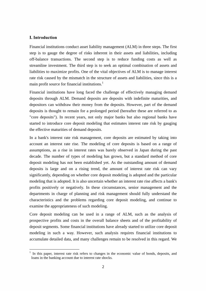
Major changes in the structure of assets and liabilities can be observed in Japanese
banks' balance sheets as of the end of fiscal 2012 relative to those as of the end of fiscal
2000 (Chart 1).2 On the asset side, corporate loans with relatively short maturities
declined from 346 trillion yen to 274 trillion yen, while housing loans and investment in
bonds such as Japanese government bonds (JGBs), whose maturities are relatively long,
increased from 70 trillion yen to 110 trillion yen and from 103 trillion yen to 212 trillion
yen, respectively. On the liability side, time deposits decreased from 301 trillion yen to
277 trillion yen because of the full removal of blanket deposit insurance in 2002 and the
following low interest rate environment that has continued to date, but demand deposits
increased substantially from 182 trillion yen to 356 trillion yen. These developments
show that it has become all the more important in ALM to properly gauge the effective
amount outstanding and maturities of core deposits.
Chart 1: Changes in Japanese banks' balance sheets
tril. yen
Ordinarydeposits
126
Housing loans70
JGBs73
Total 783
End of fiscal 2000
Loans457
Demanddeposits
182Corporate
loans346
Time deposits, etc.301
Bonds103
Other liabilities263Other assets
223
Net assets 37
tril. yen
Corporateloans274
Ordinarydeposits
299
Bonds212
JGBs167
Other liabilities223Other assets
248
Net assets 45
Total 901
End of fiscal 2012
Loans441
Demanddeposits
356
Housing loans110
Time deposits, etc.277
Source: Bank of Japan, "Financial institutions accounts" and "Deposits and loans market."
2 In Japan, the fiscal year starts in April and ends in March of the following year.
4
B. Current Situation of Interest Rate Risk Management
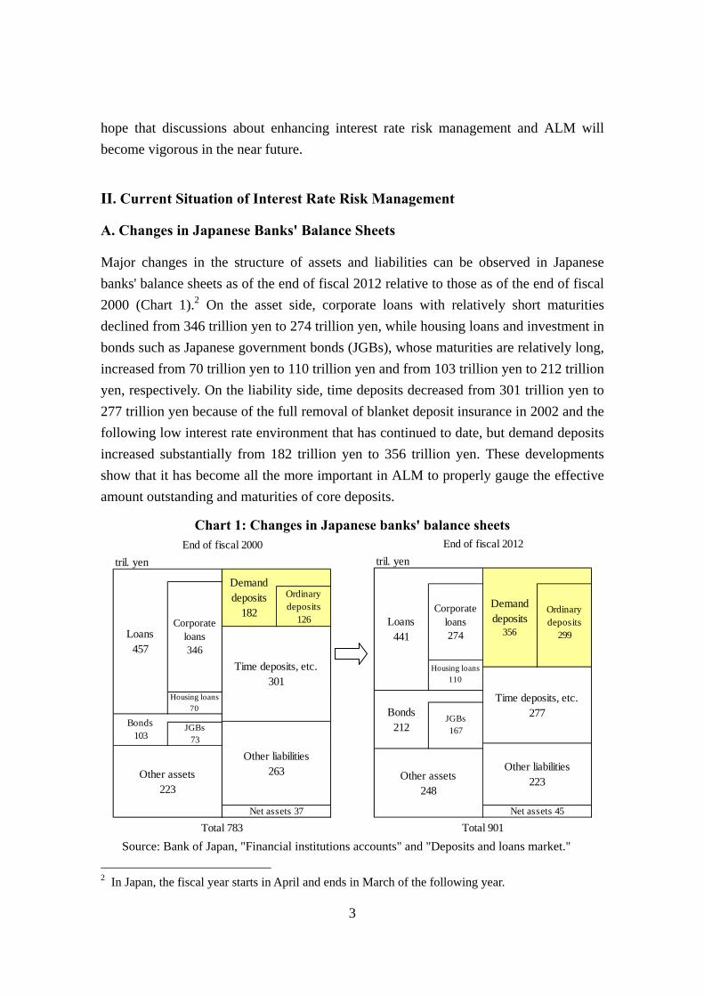
In recent years, not only major banks but also regional banks have proceeded with the
introduction of core deposit modeling as a measure to enhance ALM. According to the
Bank of Japan's survey, the number of regional banks I that introduced core deposit
modeling was three in fiscal 2006 and two in fiscal 2007, but increased thereafter and
81 percent of these banks had introduced core deposit modeling by the end of fiscal
2012. An increasing number of regional banks II and shinkin banks have also introduced
this modeling (Chart 2).3
Chart 2: Introduction of core deposit modeling1
Completion of the introduction of the modeling End of
fiscal 2008 End of
fiscal 2009End of
fiscal 2010End of
fiscal 2011 End of
fiscal 2012 Regional banks I [64]2
20 (32%) 29 (46%) 46 (73%) 51 (80%) 52 (81%)
Regional banks II [41]3
2 (5%) 6 (14%) 19 (45%) 21 (50%) 22 (54%)
Shinkin banks [261]3
3 (1%) 5 (2%) 8 (3%) 77 (29%) 96 (38%)
Notes: 1. Figures in brackets are the total at the end of fiscal 2012, and figures in parentheses are the proportions of banks that introduced core deposit modeling.
2. There were 63 regional banks I until the end of fiscal 2010. 3. There were 42 regional banks II and 262 shinkin banks until the end of fiscal 2011.
Source: Bank of Japan.
C. Effects of Core Deposits on Interest Rate Risk
While many regional banks have introduced core deposit modeling to enhance ALM, a
significant relationship between this modeling and the outlier criteria has been pointed
out (see Appendix 1 for the outlier criteria and the definition of core deposits). The
outlier criteria are defined in Basel Committee on Banking Supervision (2004) and the
guidelines by the Financial Services Agency (FSA) as the ratio of interest rate risk to
capital (Tier I + Tier II) that is more than 20 percent. The FSA's guidelines define core
deposits for measuring the interest rate risk of a banking account as demand deposits
without fixed intervals for amending applicable interest rates, deposits that can be
withdrawn at depositors' discretion, and deposits that remain at banks for a prolonged
3 As for the definition of major, regional I, regional II, and shinkin banks, see Bank of Japan (2013).
5
period. Under the guidelines, banks are required to estimate core deposits based on an
assumption of interest rate shocks. The amount outstanding of demand deposits is
assumed to decline when interest rates rise due to the outflow of money to other
financial instruments such as time deposits. Thus, the core deposits used in calculating
the outlier ratio can be taken as the amount outstanding of demand deposits with a high
probability of remaining at banks even during a phase of an interest rate rise.
Since an interest rate rise has hardly been observed in Japan during the past decade, it is
difficult to estimate the amount outstanding of core deposits during the phase of an
interest rate rise. Based on the standardized approach of the FSA's guidelines, the
duration of demand deposits is 1.25 years at the maximum.4 The duration of demand
deposits estimated by core deposit modeling tends to lengthen compared with the
standardized approach. Nevertheless, there is wide dispersion in the estimation results
of core deposit modeling depending on how the interest rate rise is incorporated in the
modeling.
Simple estimation is conducted below regarding the degree of change in the outlier ratio
depending on the estimation results of the amount outstanding of core deposits.
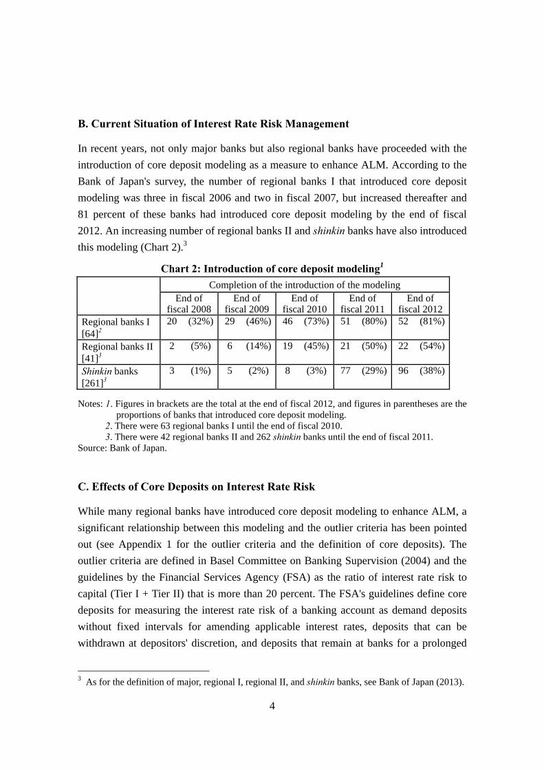
First, Chart 3 sets a sample maturity ladder by referring to the average maturity ladder
for regional banks as of the end of March 2011. Capital (Tier I + Tier II) and the amount
outstanding of demand deposits are set at 170 billion yen and 1,200 billion yen,
respectively.
Chart 3: Maturity ladders (model case) bil. yen
Amount outstanding
Less than 3M
3M–6M
6M–1Y
1Y–3Y
3Y–5Y
5Y– 7Y
7Y– 10Y
More than 10Y
Investment Loans 1,800 900 200 100 250 150 80 100 20
Bonds 700 80 70 40 150 150 60 130 20
Funding
Deposits other than demand deposits
1,300 300 250 450 250 50 0 0 0
4 While the duration of core deposits is 2.5 years at the maximum under the standardized approach, the duration of demand deposits is 1.25 years at the maximum because the maximum outstanding amount of core deposits is half of the outstanding amount of demand deposits (see Chart A-2 in Appendix 1). See Section III.A for the definition of duration.
6
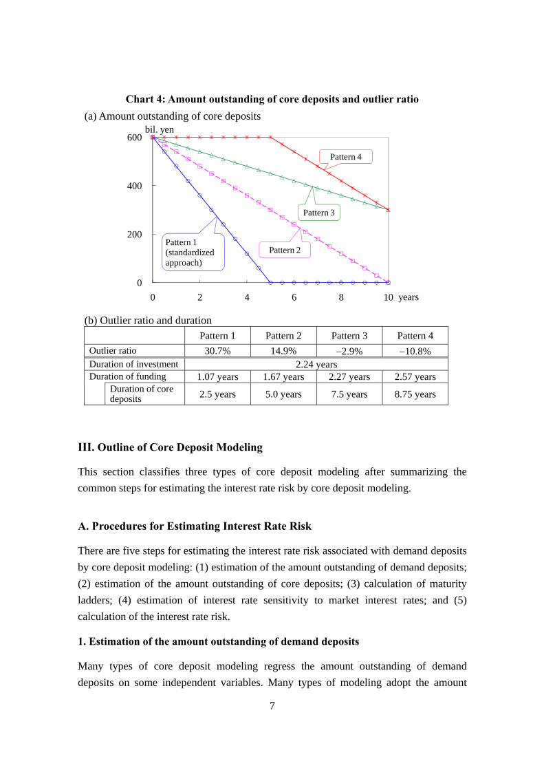
Second, Chart 4 (a) supposes four patterns for the estimated amount outstanding of core
deposits: (1) as in the standardized approach, the amount of core deposits becomes zero
after five years; (2) the amount of core deposits becomes zero after ten years; (3) the
amount of core deposits declines by half after ten years; and (4) core deposits remain
unchanged in the first five years but decline by half after ten years from the base point.5
Third, the standardized interest rate shocks are calculated at the end of March 2011
using zero coupon interest rates derived from Japanese yen LIBOR and swap interest
rates during the past six years. Changes in the zero coupon interest rate for a one-year
holding period on a rolling basis are given for the past five years. The standardized
interest rate shocks are given as the 1st and 99th percentile values of the interest rate
changes.6
The outlier ratios vary among the four patterns and are estimated to be (1) 30.7 percent,
(2) 14.9 percent, (3) minus 2.9 percent, and (4) minus 10.8 percent ("minus" indicates a
decline in the economic value of bonds, deposits, and loans when interest rates decline)
as shown in Chart 4 (b). The amount of interest rate risk differs substantially depending
on the estimated amount outstanding of core deposits.
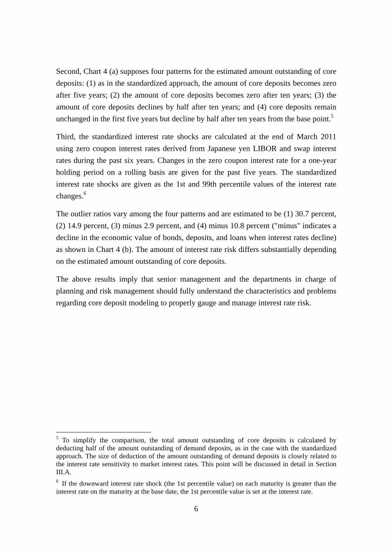
The above results imply that senior management and the departments in charge of
planning and risk management should fully understand the characteristics and problems
regarding core deposit modeling to properly gauge and manage interest rate risk.
5 To simplify the comparison, the total amount outstanding of core deposits is calculated by deducting half of the amount outstanding of demand deposits, as in the case with the standardized approach. The size of deduction of the amount outstanding of demand deposits is closely related to the interest rate sensitivity to market interest rates. This point will be discussed in detail in Section III.A. 6 If the downward interest rate shock (the 1st percentile value) on each maturity is greater than the interest rate on the maturity at the base date, the 1st percentile value is set at the interest rate.
7
Chart 4: Amount outstanding of core deposits and outlier ratio
(a) Amount outstanding of core deposits
0
200
400
600
0 2 4 6 8 10
bil. yen
years
Pattern 4
Pattern 3
Pattern 2Pattern 1(standardized approach)
(b) Outlier ratio and duration Pattern 1 Pattern 2 Pattern 3 Pattern 4
Outlier ratio 30.7% 14.9% 2.9% 10.8% Duration of investment 2.24 years Duration of funding 1.07 years 1.67 years 2.27 years 2.57 years
Duration of core deposits 2.5 years 5.0 years 7.5 years 8.75 years
III. Outline of Core Deposit Modeling
This section classifies three types of core deposit modeling after summarizing the
common steps for estimating the interest rate risk by core deposit modeling.
A. Procedures for Estimating Interest Rate Risk
There are five steps for estimating the interest rate risk associated with demand deposits
by core deposit modeling: (1) estimation of the amount outstanding of demand deposits;
(2) estimation of the amount outstanding of core deposits; (3) calculation of maturity
ladders; (4) estimation of interest rate sensitivity to market interest rates; and (5)
calculation of the interest rate risk.
1. Estimation of the amount outstanding of demand deposits
Many types of core deposit modeling regress the amount outstanding of demand
deposits on some independent variables. Many types of modeling adopt the amount
8
outstanding of demand deposits at the point of estimation, the past amount outstanding
of demand deposits (autoregressive term), economic indicators, and financial indicators
as the independent variables. In many cases, the amount outstanding of demand deposits
is estimated by type of depositors (individuals, firms, and the government). In some
cases, the amount is estimated by more detailed classification such as the amount and
type of deposits.
2. Estimation of the amount outstanding of core deposits
Based on the estimated regression in the first step, the amount outstanding of core
deposits is estimated as the amount outstanding of demand deposits that remain at banks
even during the phase of an interest rate rise. Since Japan has barely experienced an
interest rate rise during the past decade, there is a range of approaches for expressing an
interest rate rise, as described later in Section III.B. After specifying the phase of an
interest rate rise, the amount outstanding of core deposits is estimated as the amount
outstanding of demand deposits that are likely to remain at banks even during the phase
of an interest rate rise. Many types of modeling estimate the deposits that remain at
banks in each estimation period with a 99 percent confidence level as the amount
outstanding of core deposits in each estimation period.7
3. Calculation of maturity ladders
The third to fifth steps are the common steps conducted to calculate the interest rate
risk.
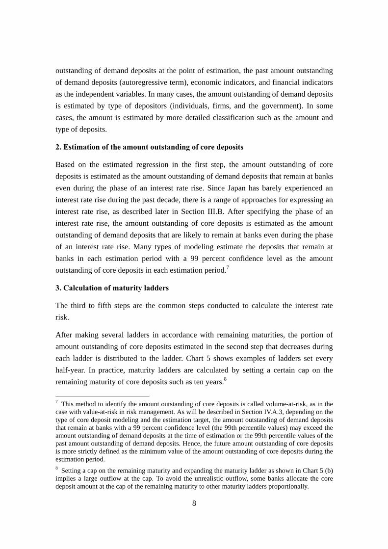
After making several ladders in accordance with remaining maturities, the portion of
amount outstanding of core deposits estimated in the second step that decreases during
each ladder is distributed to the ladder. Chart 5 shows examples of ladders set every
half-year. In practice, maturity ladders are calculated by setting a certain cap on the
remaining maturity of core deposits such as ten years.8
7 This method to identify the amount outstanding of core deposits is called volume-at-risk, as in the case with value-at-risk in risk management. As will be described in Section IV.A.3, depending on the type of core deposit modeling and the estimation target, the amount outstanding of demand deposits that remain at banks with a 99 percent confidence level (the 99th percentile values) may exceed the amount outstanding of demand deposits at the time of estimation or the 99th percentile values of the past amount outstanding of demand deposits. Hence, the future amount outstanding of core deposits is more strictly defined as the minimum value of the amount outstanding of core deposits during the estimation period. 8 Setting a cap on the remaining maturity and expanding the maturity ladder as shown in Chart 5 (b) implies a large outflow at the cap. To avoid the unrealistic outflow, some banks allocate the core deposit amount at the cap of the remaining maturity to other maturity ladders proportionally.
9
Chart 5: Amount outstanding of core deposits
(a) Proportion of the amount outstanding (b) Maturity ladders
of core deposits
0
20
40
60
80
100
0 2.5 5 7.5 10
%
years 0
10
20
30
40
50
60
0 2.5 5 7.5 10
%
years
4. Estimation of interest rate sensitivity to market interest rates
To calculate the interest rate risk associated with demand deposits, we estimate the
interest rate sensitivity to market interest rates. The interest rate sensitivity is often
estimated with regression by setting interest rates on demand deposits such as ordinary
and saving deposits as dependent variables and short-term market interest rates as an
independent variable.9
5. Calculation of the interest rate risk
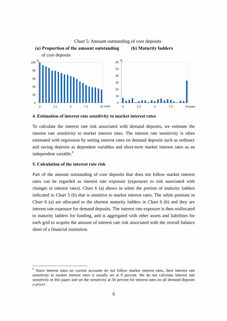
Part of the amount outstanding of core deposits that does not follow market interest
rates can be regarded as interest rate exposure (exposures to risk associated with
changes in interest rates). Chart 6 (a) shows in white the portion of maturity ladders
indicated in Chart 5 (b) that is sensitive to market interest rates. The white portions in
Chart 6 (a) are allocated to the shortest maturity ladders in Chart 6 (b) and they are
interest rate exposure for demand deposits. The interest rate exposure is then reallocated
to maturity ladders for funding, and is aggregated with other assets and liabilities for
each grid to acquire the amount of interest rate risk associated with the overall balance
sheet of a financial institution.
9 Since interest rates on current accounts do not follow market interest rates, their interest rate sensitivity to market interest rates is usually set at 0 percent. We do not calculate interest rate sensitivity in this paper and set the sensitivity at 50 percent for interest rates on all demand deposits a priori.
10
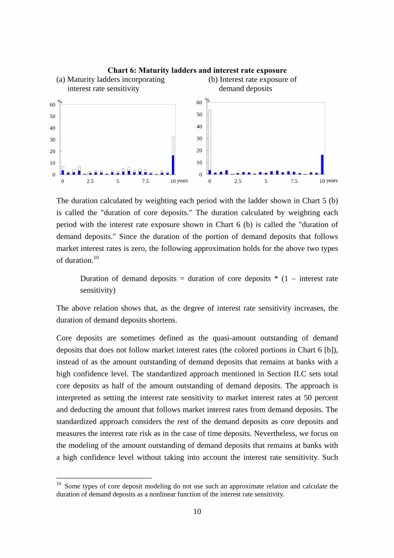
Chart 6: Maturity ladders and interest rate exposure (a) Maturity ladders incorporating (b) Interest rate exposure of
interest rate sensitivity demand deposits
0
10
20
30
40
50
60
0 2.5 5 7.5 10
%
years 0
10
20
30
40
50
60
0 2.5 5 7.5 10
%
years
The duration calculated by weighting each period with the ladder shown in Chart 5 (b)
is called the "duration of core deposits." The duration calculated by weighting each
period with the interest rate exposure shown in Chart 6 (b) is called the "duration of
demand deposits." Since the duration of the portion of demand deposits that follows
market interest rates is zero, the following approximation holds for the above two types
of duration.10
Duration of demand deposits = duration of core deposits * (1 interest rate
sensitivity)
The above relation shows that, as the degree of interest rate sensitivity increases, the
duration of demand deposits shortens.
Core deposits are sometimes defined as the quasi-amount outstanding of demand
deposits that does not follow market interest rates (the colored portions in Chart 6 [b]),
instead of as the amount outstanding of demand deposits that remains at banks with a
high confidence level. The standardized approach mentioned in Section II.C sets total
core deposits as half of the amount outstanding of demand deposits. The approach is
interpreted as setting the interest rate sensitivity to market interest rates at 50 percent
and deducting the amount that follows market interest rates from demand deposits. The
standardized approach considers the rest of the demand deposits as core deposits and
measures the interest rate risk as in the case of time deposits. Nevertheless, we focus on
the modeling of the amount outstanding of demand deposits that remains at banks with
a high confidence level without taking into account the interest rate sensitivity. Such
10 Some types of core deposit modeling do not use such an approximate relation and calculate the duration of demand deposits as a nonlinear function of the interest rate sensitivity.
11
amount outstanding is defined as the amount outstanding of core deposits as shown in
Section III.A.2.
B. Three Types of Core Deposit Modeling
There are three types of core deposit modeling in practice. These types are classified by
the assumption of the phase of an interest rate rise: (1) indirect estimation modeling; (2)
historical estimation modeling; and (3) yield-curve reference modeling.11,12,13
1. Indirect estimation modeling
As explained earlier, Japan's past data barely contain a period of interest rate rise after
the complete liberalization of deposit interest rates. The indirect estimation modeling
indirectly specifies the phase of an interest rate rise. It assumes that the past amount
outstanding of demand deposits reflects (1) the phase of a decline in interest rates and
(2) the phase of stable interest rates. It estimates both the increasing trend up in the
amount outstanding of demand deposits with phase (1) and stable trend stable in the
amount with phase (2). It specifies the declining trend down in the amount outstanding
of demand deposits during the phase of interest rate rise as
down = (stable up) stable.
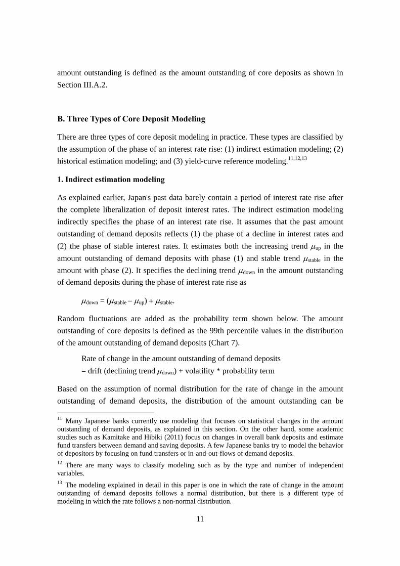
Random fluctuations are added as the probability term shown below. The amount
outstanding of core deposits is defined as the 99th percentile values in the distribution
of the amount outstanding of demand deposits (Chart 7).
Rate of change in the amount outstanding of demand deposits
= drift (declining trend down) + volatility * probability term
Based on the assumption of normal distribution for the rate of change in the amount
outstanding of demand deposits, the distribution of the amount outstanding can be
11 Many Japanese banks currently use modeling that focuses on statistical changes in the amount outstanding of demand deposits, as explained in this section. On the other hand, some academic studies such as Kamitake and Hibiki (2011) focus on changes in overall bank deposits and estimate fund transfers between demand and saving deposits. A few Japanese banks try to model the behavior of depositors by focusing on fund transfers or in-and-out-flows of demand deposits. 12 There are many ways to classify modeling such as by the type and number of independent variables. 13 The modeling explained in detail in this paper is one in which the rate of change in the amount outstanding of demand deposits follows a normal distribution, but there is a different type of modeling in which the rate follows a non-normal distribution.
12
specified if the drift (expected value) and volatility (standard deviation) are determined,
and the 99th percentile values of the amount outstanding of demand deposits can be
analytically calculated without simulation.14 See Appendix 2 for a concrete model.
Chart 7: Amount outstanding of core deposits in indirect estimation modeling1
0
20
40
60
80
100
120
-2 0 2 4 6 8 10 years
Amount outstanding of core deposits at a phase of interest rate rise (99th percentile values)
Amount outstanding of demand deposits at a phase of interest rate rise (expected value)
Actual amount
Note: 1. The amount outstanding of demand deposits at the base date is set at 100.
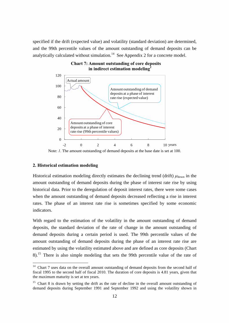
2. Historical estimation modeling
Historical estimation modeling directly estimates the declining trend (drift) down in the
amount outstanding of demand deposits during the phase of interest rate rise by using
historical data. Prior to the deregulation of deposit interest rates, there were some cases
when the amount outstanding of demand deposits decreased reflecting a rise in interest
rates. The phase of an interest rate rise is sometimes specified by some economic
indicators.
With regard to the estimation of the volatility in the amount outstanding of demand
deposits, the standard deviation of the rate of change in the amount outstanding of
demand deposits during a certain period is used. The 99th percentile values of the
amount outstanding of demand deposits during the phase of an interest rate rise are
estimated by using the volatility estimated above and are defined as core deposits (Chart
8).15 There is also simple modeling that sets the 99th percentile value of the rate of
14 Chart 7 uses data on the overall amount outstanding of demand deposits from the second half of fiscal 1995 to the second half of fiscal 2010. The duration of core deposits is 4.81 years, given that the maximum maturity is set at ten years. 15 Chart 8 is drawn by setting the drift as the rate of decline in the overall amount outstanding of demand deposits during September 1991 and September 1992 and using the volatility shown in
13
change in the amount outstanding of demand deposits during a certain period as the drift
and does not take account of the volatility.
Chart 8: Amount outstanding of core deposits in historical estimation modeling1
0
20
40
60
80
100
120
-2 0 2 4 6 8 10 years
Amount outstanding of core deposits at a phase of interest rate rise (99th percentile values)
Amount outstanding of demand deposits at a phase of interest rate rise (expected value)
Actual amount
Note: 1. The amount outstanding of demand deposits at the base date is set at 100.
3. Yield-curve reference modeling
Yield-curve reference modeling uses the current yield curve to express the phase of an
interest rate rise. The yield curve with an upward slope indicates a rise in the implied
forward interest rate. This is the phase of an interest rate rise.
The rate of change in the amount outstanding of demand deposits regresses on interest
rates. To estimate the future amount outstanding of demand deposits, stochastic interest
rates based on the current yield curve are used for the interest rate variable. 16
Independent variables other than the interest rate variable are often fixed with the
present values.17
Rate of change in the amount outstanding of demand deposits
= β0 + β1 * interest rate variable + β2 * other variables … + disturbance terms
Chart 7. The duration of core deposits is 6.35 years, given that the maximum maturity is set at ten years. 16 Some preceding studies such as Jarrow and van Deventer (1998) also use market interest rates as independent variables. 17 A range of economic indicators is used as independent variables other than interest rates. There is also modeling that only uses market interest rates and an autoregressive term (the past amount outstanding of demand deposits or its rate of change) as independent variables.
14
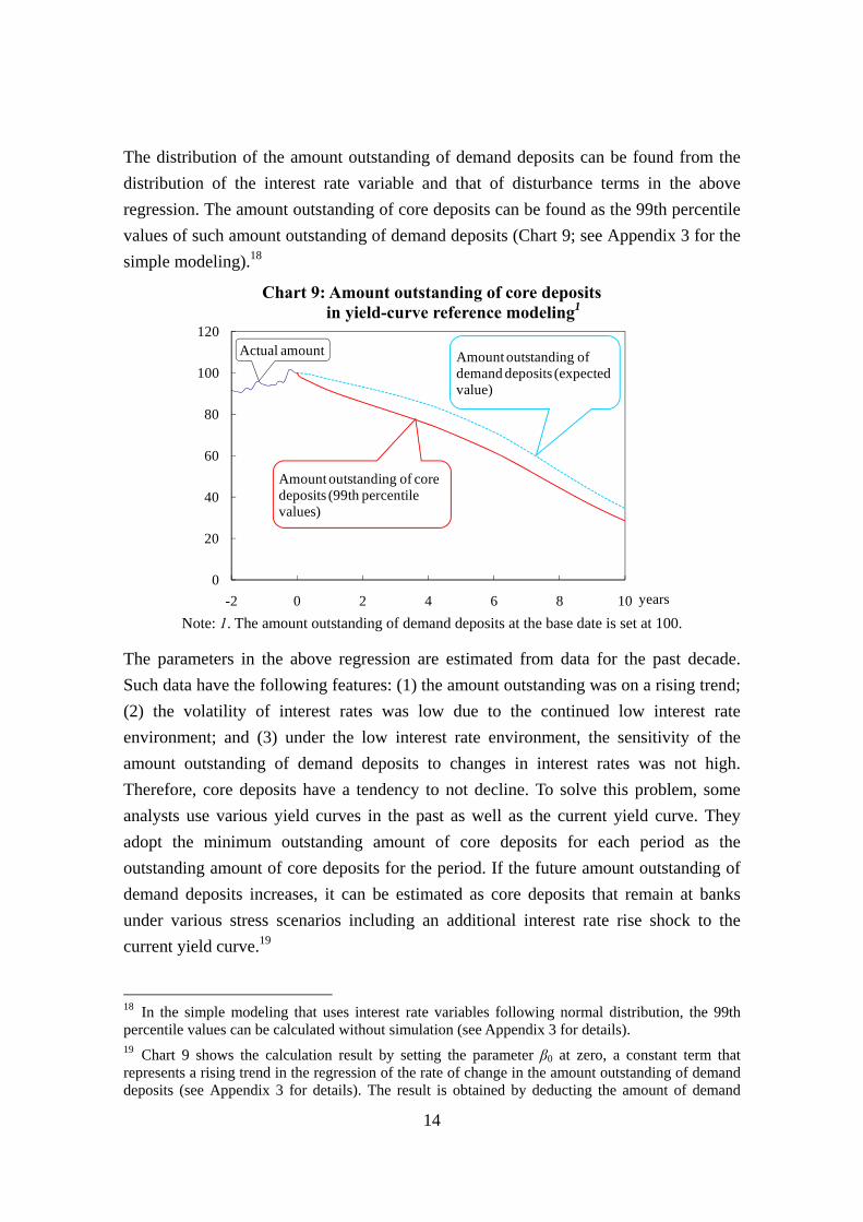
The distribution of the amount outstanding of demand deposits can be found from the
distribution of the interest rate variable and that of disturbance terms in the above
regression. The amount outstanding of core deposits can be found as the 99th percentile
values of such amount outstanding of demand deposits (Chart 9; see Appendix 3 for the
simple modeling).18
Chart 9: Amount outstanding of core deposits in yield-curve reference modeling1
0
20
40
60
80
100
120
-2 0 2 4 6 8 10 years
Actual amount Amount outstanding of demand deposits (expected value)
Amount outstanding of core deposits (99th percentile values)
Note: 1. The amount outstanding of demand deposits at the base date is set at 100.
The parameters in the above regression are estimated from data for the past decade.
Such data have the following features: (1) the amount outstanding was on a rising trend;
(2) the volatility of interest rates was low due to the continued low interest rate
environment; and (3) under the low interest rate environment, the sensitivity of the
amount outstanding of demand deposits to changes in interest rates was not high.
Therefore, core deposits have a tendency to not decline. To solve this problem, some
analysts use various yield curves in the past as well as the current yield curve. They
adopt the minimum outstanding amount of core deposits for each period as the
outstanding amount of core deposits for the period. If the future amount outstanding of
demand deposits increases, it can be estimated as core deposits that remain at banks
under various stress scenarios including an additional interest rate rise shock to the
current yield curve.19
18 In the simple modeling that uses interest rate variables following normal distribution, the 99th percentile values can be calculated without simulation (see Appendix 3 for details). 19 Chart 9 shows the calculation result by setting the parameter β0 at zero, a constant term that represents a rising trend in the regression of the rate of change in the amount outstanding of demand deposits (see Appendix 3 for details). The result is obtained by deducting the amount of demand
15
IV. Interest Rate Risk Management Using Core Deposit Modeling
This section explains problems regarding interest rate risk management using core
deposit modeling. These problems should be shared among senior management and the
departments in charge of planning and risk management.
A. Problems regarding Core Deposit Modeling
The following three points should be noted regarding the amount outstanding of core
deposits calculated by core deposit modeling.
1. Differences in assumptions of modeling
In Japan, as mentioned earlier, core deposit modeling has been conducted based on
various assumptions since a rise in interest rates was barely observed in Japan for the
past decade.
For example, the indirect estimation modeling assumes a decline in the amount
outstanding of demand deposits (a phase of a rise in interest rates) by using the rise in
the amount outstanding in symmetric. Thus, if the rise in the amount outstanding is
large, the duration of core deposits turns out to be short. In the historical estimation
modeling, the duration of core deposits tends to be relatively long, if there are no large
declines in the amount outstanding of demand deposits in the past data. In the
yield-curve reference modeling, the amount outstanding of demand deposits tends to
increase for a time, as will be discussed in Section IV.A.3. Therefore, the duration of
core deposits tends to be long.
In using core deposit modeling, it is necessary to first examine whether the assumptions
of the modeling are appropriate in light of the objective of using the modeling for
interest rate risk management. It is also important to check whether parameters are
properly set in line with the objective. In addition, the senior management needs to
examine whether the amount outstanding of core deposits is appropriate in view of their
experience. Financial institutions are required to gauge risks from multiple perspectives
by comparing with other methods.
deposits that rose due to factors other than changes in interest rates. The duration of core deposits is 6.57 years, given that the maximum maturity is set at ten years.
16
2. Stability in estimation results
The estimation results of core deposit modeling are sometimes unstable, and this
problem is a significant challenge faced by financial institutions that employ core
deposit modeling.
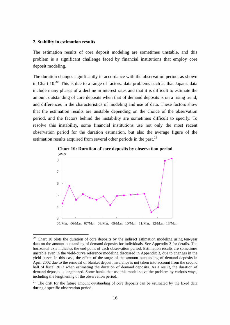
The duration changes significantly in accordance with the observation period, as shown
in Chart 10.20 This is due to a range of factors: data problems such as that Japan's data
include many phases of a decline in interest rates and that it is difficult to estimate the
amount outstanding of core deposits when that of demand deposits is on a rising trend;
and differences in the characteristics of modeling and use of data. These factors show
that the estimation results are unstable depending on the choice of the observation
period, and the factors behind the instability are sometimes difficult to specify. To
resolve this instability, some financial institutions use not only the most recent
observation period for the duration estimation, but also the average figure of the
estimation results acquired from several other periods in the past.21
Chart 10: Duration of core deposits by observation period
3
4
5
6
7
8
05/Mar. 06/Mar. 07/Mar. 08/Mar. 09/Mar. 10/Mar. 11/Mar. 12/Mar. 13/Mar.
years
20 Chart 10 plots the duration of core deposits by the indirect estimation modeling using ten-year data on the amount outstanding of demand deposits for individuals. See Appendix 2 for details. The horizontal axis indicates the end point of each observation period. Estimation results are sometimes unstable even in the yield-curve reference modeling discussed in Appendix 3, due to changes in the yield curve. In this case, the effect of the surge of the amount outstanding of demand deposits in April 2002 due to the removal of blanket deposit insurance is not taken into account from the second half of fiscal 2012 when estimating the duration of demand deposits. As a result, the duration of demand deposits is lengthened. Some banks that use this model solve the problem by various ways, including the lengthening of the observation period. 21 The drift for the future amount outstanding of core deposits can be estimated by the fixed data during a specific observation period.
17
As the parameters of risk econometric modeling depend on the observation periods, it is
important for financial institutions to understand sufficiently the characteristics of core
deposit modeling and cover the instability by, for example, using fixed parameters for a
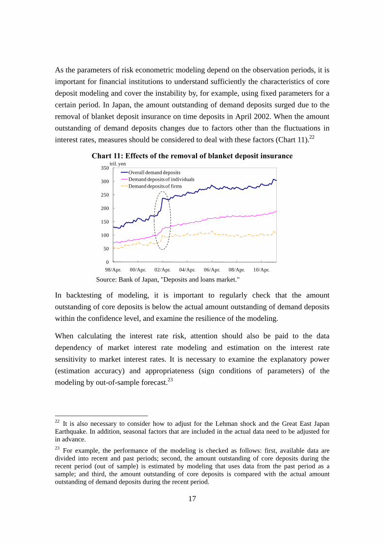
certain period. In Japan, the amount outstanding of demand deposits surged due to the
removal of blanket deposit insurance on time deposits in April 2002. When the amount
outstanding of demand deposits changes due to factors other than the fluctuations in
interest rates, measures should be considered to deal with these factors (Chart 11).22
Chart 11: Effects of the removal of blanket deposit insurance
0
50
100
150
200
250
300
350
98/Apr. 00/Apr. 02/Apr. 04/Apr. 06/Apr. 08/Apr. 10/Apr.
tril. yen
Overall demand depositsDemand deposits of individualsDemand deposits of firms
Source: Bank of Japan, "Deposits and loans market."
In backtesting of modeling, it is important to regularly check that the amount
outstanding of core deposits is below the actual amount outstanding of demand deposits
within the confidence level, and examine the resilience of the modeling.
When calculating the interest rate risk, attention should also be paid to the data
dependency of market interest rate modeling and estimation on the interest rate
sensitivity to market interest rates. It is necessary to examine the explanatory power
(estimation accuracy) and appropriateness (sign conditions of parameters) of the
modeling by out-of-sample forecast.23
22 It is also necessary to consider how to adjust for the Lehman shock and the Great East Japan Earthquake. In addition, seasonal factors that are included in the actual data need to be adjusted for in advance. 23 For example, the performance of the modeling is checked as follows: first, available data are divided into recent and past periods; second, the amount outstanding of core deposits during the recent period (out of sample) is estimated by modeling that uses data from the past period as a sample; and third, the amount outstanding of core deposits is compared with the actual amount outstanding of demand deposits during the recent period.
18
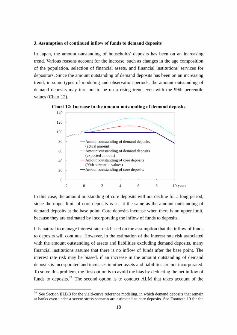
3. Assumption of continued inflow of funds to demand deposits
In Japan, the amount outstanding of households' deposits has been on an increasing
trend. Various reasons account for the increase, such as changes in the age composition
of the population, selection of financial assets, and financial institutions' services for
depositors. Since the amount outstanding of demand deposits has been on an increasing
trend, in some types of modeling and observation periods, the amount outstanding of
demand deposits may turn out to be on a rising trend even with the 99th percentile
values (Chart 12).
Chart 12: Increase in the amount outstanding of demand deposits
0
20
40
60
80
100
120
140
-2 0 2 4 6 8 10 years
Amount outstanding of demand deposits(actual amount)Amount outstanding of demand deposits (expected amount)Amount outstanding of core deposits (99th percentile values)Amount outstanding of core deposits
In this case, the amount outstanding of core deposits will not decline for a long period,
since the upper limit of core deposits is set at the same as the amount outstanding of
demand deposits at the base point. Core deposits increase when there is no upper limit,
because they are estimated by incorporating the inflow of funds to deposits.
It is natural to manage interest rate risk based on the assumption that the inflow of funds
to deposits will continue. However, in the estimation of the interest rate risk associated
with the amount outstanding of assets and liabilities excluding demand deposits, many
financial institutions assume that there is no inflow of funds after the base point. The
interest rate risk may be biased, if an increase in the amount outstanding of demand
deposits is incorporated and increases in other assets and liabilities are not incorporated.
To solve this problem, the first option is to avoid the bias by deducting the net inflow of
funds to deposits.24 The second option is to conduct ALM that takes account of the
24 See Section III.B.3 for the yield-curve reference modeling, in which demand deposits that remain at banks even under a severe stress scenario are estimated as core deposits. See Footnote 19 for the
19
future inflow of funds, prepayment, and rollovers for all assets and liabilities.
Nevertheless, the second option is a major challenge faced by financial institutions in
terms of ALM. Enhancement of core deposit modeling is a step toward resolving such a
challenge, as will be discussed in Section V.A.
B. Problems regarding Estimation of Interest Rate Risk
Three points should be noted when estimating interest rate risk from the maturity
ladders calculated by the core deposit modeling.
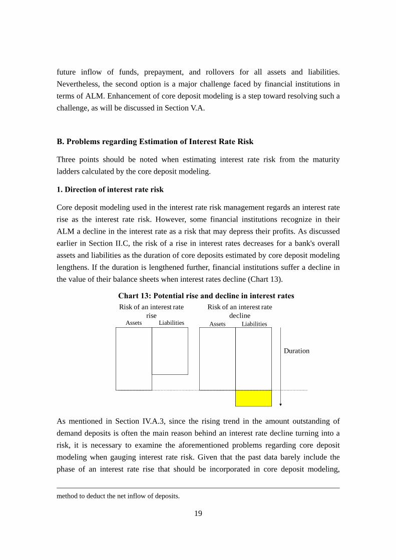
1. Direction of interest rate risk
Core deposit modeling used in the interest rate risk management regards an interest rate
rise as the interest rate risk. However, some financial institutions recognize in their
ALM a decline in the interest rate as a risk that may depress their profits. As discussed
earlier in Section II.C, the risk of a rise in interest rates decreases for a bank's overall
assets and liabilities as the duration of core deposits estimated by core deposit modeling
lengthens. If the duration is lengthened further, financial institutions suffer a decline in
the value of their balance sheets when interest rates decline (Chart 13).
Chart 13: Potential rise and decline in interest rates Risk of an interest rate
riseRisk of an interest rate
declineAssets LiabilitiesAssets Liabilities
Duration
As mentioned in Section IV.A.3, since the rising trend in the amount outstanding of
demand deposits is often the main reason behind an interest rate decline turning into a
risk, it is necessary to examine the aforementioned problems regarding core deposit
modeling when gauging interest rate risk. Given that the past data barely include the
phase of an interest rate rise that should be incorporated in core deposit modeling,
method to deduct the net inflow of deposits.
20
financial institutions need to sufficiently conduct stress testing without depending on the
past data.25 When the risk of an interest rate decline is confirmed, some financial
institutions may consider the hedge operations against the risk. In conducting the hedge
operations, the financial institutions are required to deliberate, for example, on setting
risk limits on bond investment and interest rate swaps as well as on the total portfolio by
examining the size of risk, including the effects on their earnings.26
2. Changes in interest rate sensitivity
This paper focuses on the variety of the maturity structure of core deposits in each
model, and sets the interest rate sensitivity of demand deposits to market interest rates at
a fixed level of 50 percent. However, interest rate risk depends significantly on the
interest rate sensitivity, and thus it is necessary to assess interest rate risk by taking into
account future changes in the sensitivity. For example, when the sensitivity approaches
100 percent, the interest rate exposure of most of the amount of demand deposits
concentrates at the shortest maturity, reducing the duration of demand deposits. Even
when a decline in interest rates decreases the value of financial institutions' balance
sheets as mentioned in Section IV.B.1, the risk changes to an interest rate rise if the
sensitivity exceeds 50 percent. Financial institutions are required to make a risk
assessment by taking account of possible changes in the interest rate sensitivity via
stress testing, which was mentioned earlier.
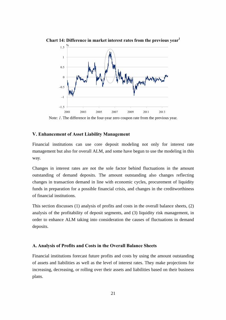
3. Observation period for interest rate shocks
The 1–99 percentile values that are used as interest rate shocks in calculating the outlier
ratio and VaR are usually based on certain observation periods. For instance, Japan
experienced large fluctuations in interest rates around 2006 because of expectations
regarding termination of the zero interest rate policy. If such data are not included in the
observation period, the range of the interest rate shocks of 1–99 percentile values
narrows and the interest rate risk decreases (Chart 14). It is therefore necessary to
recognize the possibility that such a shock observed more than five years ago will occur
again, and to gauge interest rate risk without depending on a certain observation period.
25 It may be insufficient to use only the past rise in interest rates as the stress scenario. 26 The economic value of deposits and loans is not recorded as gains/losses in financial accounting. However, it should be noted that the economic value of bonds and interest rate swaps directly affects gains/losses in financial accounting.
21
Chart 14: Difference in market interest rates from the previous year1
%
Note: 1. The difference in the four-year zero coupon rate from the previous year.
V. Enhancement of Asset Liability Management
Financial institutions can use core deposit modeling not only for interest rate
management but also for overall ALM, and some have begun to use the modeling in this
way.
Changes in interest rates are not the sole factor behind fluctuations in the amount
outstanding of demand deposits. The amount outstanding also changes reflecting
changes in transaction demand in line with economic cycles, procurement of liquidity
funds in preparation for a possible financial crisis, and changes in the creditworthiness
of financial institutions.
This section discusses (1) analysis of profits and costs in the overall balance sheets, (2)
analysis of the profitability of deposit segments, and (3) liquidity risk management, in
order to enhance ALM taking into consideration the causes of fluctuations in demand
deposits.
A. Analysis of Profits and Costs in the Overall Balance Sheets
Financial institutions forecast future profits and costs by using the amount outstanding
of assets and liabilities as well as the level of interest rates. They make projections for
increasing, decreasing, or rolling over their assets and liabilities based on their business
plans.
22
Since it is difficult for financial institutions to control the amount of demand deposits,
they often use the approximations in their business plans. If they use the method of
estimating the amount outstanding of demand deposits by core deposit modeling
discussed in Section III.A.1, they may be able to estimate the amount outstanding more
objectively. They can also adopt variables such as economic developments projected in
their business plans as independent variables in the modeling.
Given such problems, to analyze profits and costs in the overall balance sheets, financial
institutions need to take into account rollovers and early redemptions that are
incorporated in the estimation of the amount outstanding of demand deposits, in the
case of other assets and liabilities including time deposits, corporate loans, and housing
loans.
B. Analysis of Profitability of Deposit Segments
Demand deposits such as ordinary deposits are a means for financial institutions to
acquire funds at relatively low interest rates. If demand deposits remain at these
institutions for a prolonged period, this will expand their profits.
Financial institutions are expected to analyze the profitability of their demand deposits
by type of deposits and depositors. For example, individual deposits can be classified by
amount, year of transaction, occupation, age, gender, family structure, and usage of
Internet banking. Corporate deposits can be classified by industry and the relationship
including loans.27 Regional financial institutions can monitor the changes in population
of their local areas. Financial institutions will be able to enhance their profitability if
they (1) analyze the segments in which the duration of demand deposits lengthens and
the factors behind changes in the amount outstanding of demand deposits, and (2)
strengthen their business strategies for the segment in which demand deposits tend to
remain for a prolonged period as core deposits. To conduct such an analysis, financial
institutions should continue accumulating sufficient data on demand deposits.
27 Among several attributions, the attribution of age has a large impact on the amount of individual deposits. The attribution of transaction year has a large impact on the amount of corporate deposits. Some regional financial institutions try to monitor the cash flow of each demand deposit.
23
C. Liquidity Risk Management
When financial institutions' creditworthiness declines, depositors are expected to
respond instantly and withdraw money from deposits.28 Many financial institutions
have already introduced liquidity risk management that assumes a stress scenario
regarding such illiquidity. If financial institutions can estimate the amount outstanding
of demand deposits based on their creditworthiness, it is possible for them to implement
countermeasures against the outflow of liquidity caused by credit concerns.29
The idea in core deposit modeling can be applied to liquidity risk management. In fact,
Ito and Kijima (2007) proposed to model credit risk factors of a drop in the amount
outstanding of demand deposits in response to changes in the creditworthiness of
financial institutions. The credit risk factors can be regularly monitored by depositors
such as credit ratings and corporate bond prices. Changes in such past data are assumed
to be used in the modeling. On the other hand, stress testing based on various scenarios
can cover a sudden change in financial institutions' creditworthiness or large-scale
disruptions in financial markets and the payment and settlement systems that cannot be
forecasted from the past data on the credit risk factors.
VI. Conclusion
We explained the characteristics and problems regarding various types of core deposit
modeling, which has increasingly been introduced at major and regional banks. We then
discussed issues related to the enhancement of ALM to analyze future profits and costs
in the overall balance sheets and the profitability of deposit segments.
Nevertheless, Japan faces a large constraint on available data because it has barely
experienced an interest rate rise during the past decade. Thus, a standard method for
core deposit modeling has not been established yet, and the resilience of the modeling
has not been examined thoroughly. It is expected that surveys and research on core
deposit modeling will develop further to improve interest rate risk management using
core deposit modeling and enhance ALM.
28 Deposits for payment and settlement are fully protected if they meet all the following conditions: deposits with no interest rates, demand deposits, and deposits used for payment and settlement. 29 Some banks monitor the outflow of demand deposits of some Japanese banks during the Japanese bank crisis that occurred between 1997 and 1999 and that of some Greek banks during the European debt crisis that occurred between 2010 and 2012.
24
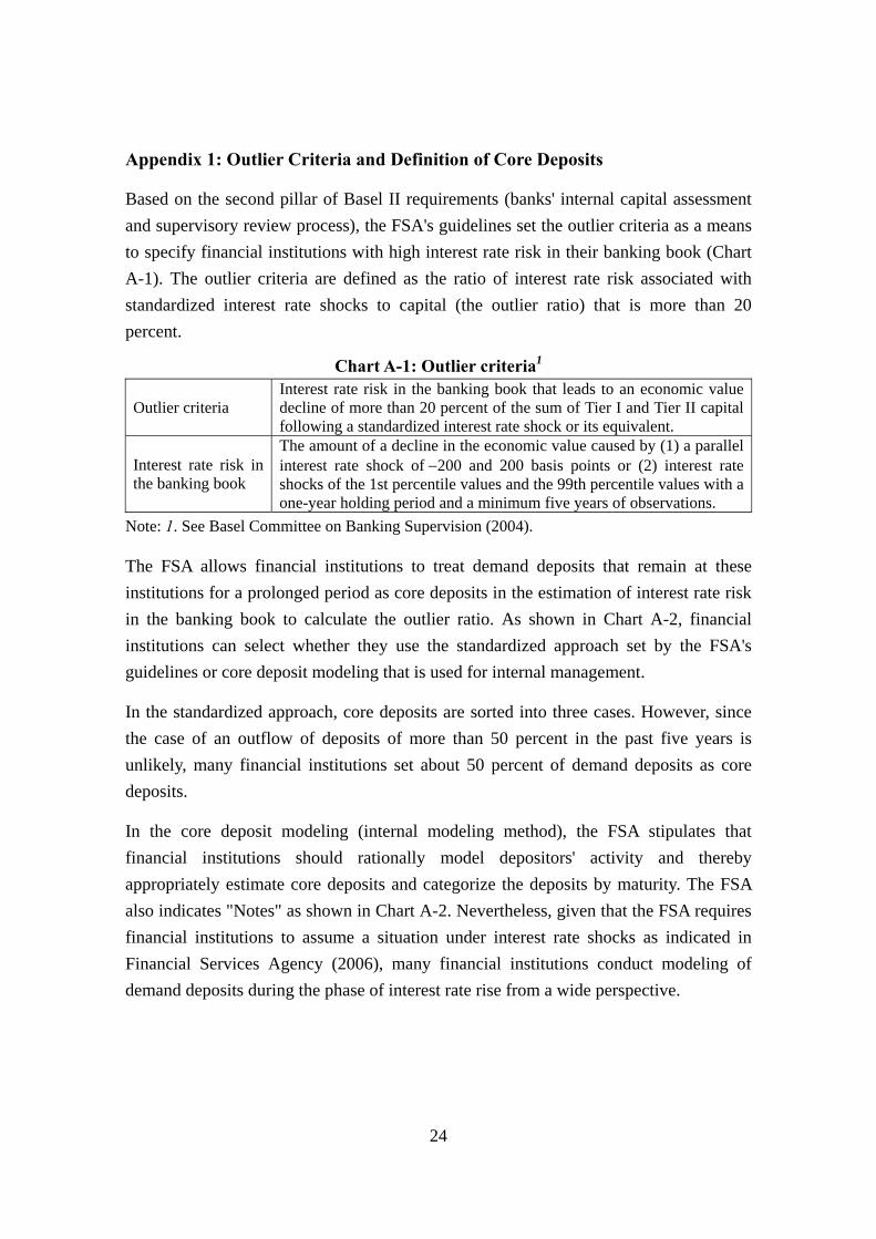
Appendix 1: Outlier Criteria and Definition of Core Deposits
Based on the second pillar of Basel II requirements (banks' internal capital assessment
and supervisory review process), the FSA's guidelines set the outlier criteria as a means
to specify financial institutions with high interest rate risk in their banking book (Chart
A-1). The outlier criteria are defined as the ratio of interest rate risk associated with
standardized interest rate shocks to capital (the outlier ratio) that is more than 20
percent.
Chart A-1: Outlier criteria1
Outlier criteria Interest rate risk in the banking book that leads to an economic value decline of more than 20 percent of the sum of Tier I and Tier II capital following a standardized interest rate shock or its equivalent.
Interest rate risk in the banking book
The amount of a decline in the economic value caused by (1) a parallel interest rate shock of200 and 200 basis points or (2) interest rate shocks of the 1st percentile values and the 99th percentile values with a one-year holding period and a minimum five years of observations.
Note: 1. See Basel Committee on Banking Supervision (2004).
The FSA allows financial institutions to treat demand deposits that remain at these
institutions for a prolonged period as core deposits in the estimation of interest rate risk
in the banking book to calculate the outlier ratio. As shown in Chart A-2, financial
institutions can select whether they use the standardized approach set by the FSA's
guidelines or core deposit modeling that is used for internal management.
In the standardized approach, core deposits are sorted into three cases. However, since
the case of an outflow of deposits of more than 50 percent in the past five years is
unlikely, many financial institutions set about 50 percent of demand deposits as core
deposits.
In the core deposit modeling (internal modeling method), the FSA stipulates that
financial institutions should rationally model depositors' activity and thereby
appropriately estimate core deposits and categorize the deposits by maturity. The FSA
also indicates "Notes" as shown in Chart A-2. Nevertheless, given that the FSA requires
financial institutions to assume a situation under interest rate shocks as indicated in
Financial Services Agency (2006), many financial institutions conduct modeling of
demand deposits during the phase of interest rate rise from a wide perspective.

25
Chart A-2: Definition of core deposits and types of modeling
Concept of core deposits
Demand deposits without fixed intervals for amending applicable interest rates, the deposits that can be withdrawn at depositors' discretion, and the deposits that remain at banks for a prolonged period.
Definition of core deposits
Standardized approach
a. Banks define core deposits as the lowest amount of demand deposits among (1) the lowest amount outstanding during the past five years, (2) the amount outstanding calculated by deducting the largest outflow of funds during the past five years from the current amount outstanding of demand deposits, and (3) about 50 percent of the current amount outstanding of demand deposits, and set the lowest amount as the upper limit. They can set the maturity within five years (within 2.5 years on average).
Internal modeling approach
b. Banks define core deposits by rationally modeling depositors' activity and thereby appropriately estimating core deposits and categorizing the deposits by maturity.
Notes
Banks should understand that the interest rate risk fluctuates significantly depending on the definition of core deposits, appropriately define core deposits, and examine the modeling by backtesting.
Banks should continue to use the definition they chose unless there is a rational reason to terminate the use.
Banks are allowed to use an advanced method of calculating interest rate risk based on core deposit modeling that is used internally, on the condition that they can explain to the FSA the rationality of using the modeling.
26
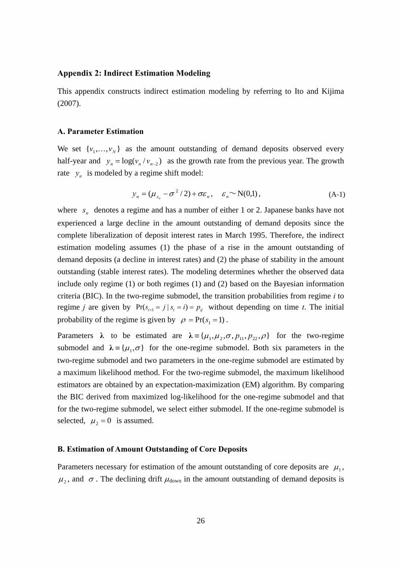
Appendix 2: Indirect Estimation Modeling
This appendix constructs indirect estimation modeling by referring to Ito and Kijima
(2007).
A. Parameter Estimation
We set },,{ 1 Nvv as the amount outstanding of demand deposits observed every
half-year and )/log( 2 nnn vvy as the growth rate from the previous year. The growth
rate ny is modeled by a regime shift model:
nsn ny )2/( 2 , )1,0N(~n , (A-1)
where ns denotes a regime and has a number of either 1 or 2. Japanese banks have not
experienced a large decline in the amount outstanding of demand deposits since the
complete liberalization of deposit interest rates in March 1995. Therefore, the indirect
estimation modeling assumes (1) the phase of a rise in the amount outstanding of
demand deposits (a decline in interest rates) and (2) the phase of stability in the amount
outstanding (stable interest rates). The modeling determines whether the observed data
include only regime (1) or both regimes (1) and (2) based on the Bayesian information
criteria (BIC). In the two-regime submodel, the transition probabilities from regime i to regime j are given by ijtt pisjs )|Pr( 1 without depending on time t. The initial
probability of the regime is given by )1Pr( 1 s .
Parameters λ to be estimated are },,,,,{ 221121 ppλ for the two-regime
submodel and },{ 1 λ for the one-regime submodel. Both six parameters in the
two-regime submodel and two parameters in the one-regime submodel are estimated by
a maximum likelihood method. For the two-regime submodel, the maximum likelihood
estimators are obtained by an expectation-maximization (EM) algorithm. By comparing
the BIC derived from maximized log-likelihood for the one-regime submodel and that
for the two-regime submodel, we select either submodel. If the one-regime submodel is
selected, 02 is assumed.
B. Estimation of Amount Outstanding of Core Deposits
Parameters necessary for estimation of the amount outstanding of core deposits are 1 ,
2 , and . The declining drift down in the amount outstanding of demand deposits is
27
given as30
12212down 2)( . (A-2)
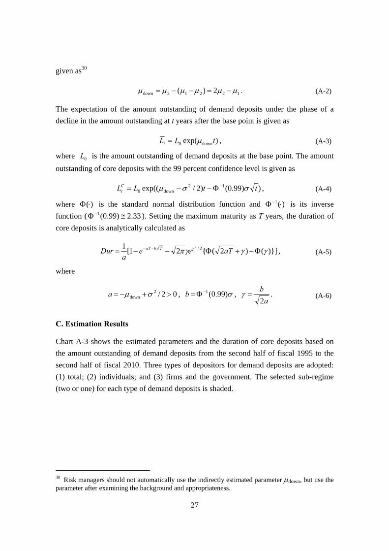
The expectation of the amount outstanding of demand deposits under the phase of a
decline in the amount outstanding at t years after the base point is given as
)exp( down0 tLLt , (A-3)
where 0L is the amount outstanding of demand deposits at the base point. The amount
outstanding of core deposits with the 99 percent confidence level is given as
))99.0()2/exp(( 12down0 ttLLC
t , (A-4)
where )( is the standard normal distribution function and )(1 is its inverse
function ( 33.2)99.0(1 ). Setting the maximum maturity as T years, the duration of
core deposits is analytically calculated as
)}]()2({21[1 2/2
aTeea
Dur TbaT , (A-5)
where
02/2down a , )99.0( 1b ,
a
b
2 . (A-6)
C. Estimation Results
Chart A-3 shows the estimated parameters and the duration of core deposits based on
the amount outstanding of demand deposits from the second half of fiscal 1995 to the
second half of fiscal 2010. Three types of depositors for demand deposits are adopted:
(1) total; (2) individuals; and (3) firms and the government. The selected sub-regime
(two or one) for each type of demand deposits is shaded.
30 Risk managers should not automatically use the indirectly estimated parameter down, but use the parameter after examining the background and appropriateness.

28
Chart A-3: Results based on second half of fiscal 1995–second half of fiscal 2010
Depositors Two regimes One regime
down Duration(years)
1 2 1
Total 0.213 0.045 0.041 0.067 0.069 0.124 0.041 4.81
Individuals 0.228 0.067 0.040 0.090 0.069 0.095 0.040 5.40
Firms and the government 0.264 0.017 0.049 0.047 0.090 0.227 0.049 3.28
Chart 7 plots the expected amount outstanding of demand deposits and the amount
outstanding of core deposits with the parameters 0.124down and 0.041 ,
which are estimated using the total amount outstanding of demand deposits in Chart
A-3.
Chart 10 plots the duration of core deposits using ten-year data on the amount
outstanding of demand deposits for individuals.
29
Appendix 3: Yield-Curve Reference Modeling
This appendix constructs an example of yield-curve reference modeling by referring to
Okubo et al. (2010).
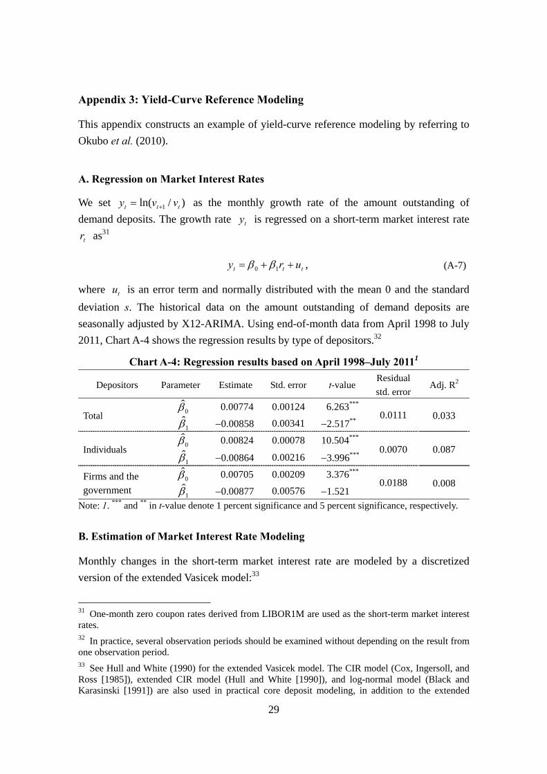
A. Regression on Market Interest Rates
We set )/ln( 1 ttt vvy as the monthly growth rate of the amount outstanding of
demand deposits. The growth rate ty is regressed on a short-term market interest rate
tr as31
ttt ury 10 , (A-7)
where tu is an error term and normally distributed with the mean 0 and the standard
deviation s. The historical data on the amount outstanding of demand deposits are
seasonally adjusted by X12-ARIMA. Using end-of-month data from April 1998 to July
2011, Chart A-4 shows the regression results by type of depositors.32
Chart A-4: Regression results based on April 1998–July 20111
Depositors Parameter Estimate Std. error t-value Residual
std. error Adj. R2
Total 0 0.00774 0.00124 6.263***
0.0111 0.033 1 0.00858 0.00341 2.517**
Individuals 0 0.00824 0.00078 10.504***
0.0070 0.087 1 0.00864 0.00216 3.996***
Firms and the government
0 0.00705 0.00209 3.376*** 0.0188 0.008
1 0.00877 0.00576 1.521
Note: 1. *** and ** in t-value denote 1 percent significance and 5 percent significance, respectively.
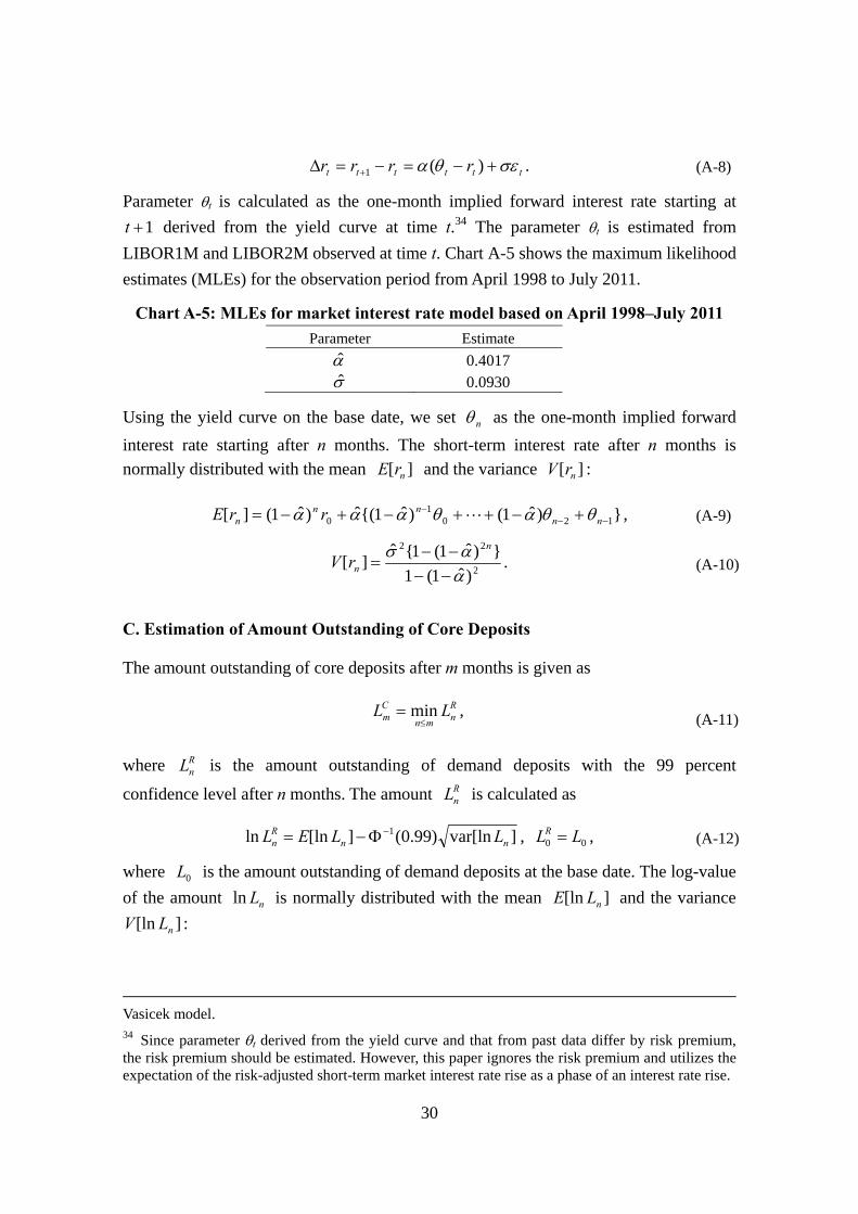
B. Estimation of Market Interest Rate Modeling
Monthly changes in the short-term market interest rate are modeled by a discretized
version of the extended Vasicek model:33
31 One-month zero coupon rates derived from LIBOR1M are used as the short-term market interest rates. 32 In practice, several observation periods should be examined without depending on the result from one observation period. 33 See Hull and White (1990) for the extended Vasicek model. The CIR model (Cox, Ingersoll, and Ross [1985]), extended CIR model (Hull and White [1990]), and log-normal model (Black and Karasinski [1991]) are also used in practical core deposit modeling, in addition to the extended
30
tttttt rrrr )(1 . (A-8)
Parameter t is calculated as the one-month implied forward interest rate starting at
1t derived from the yield curve at time t.34 The parameter t is estimated from
LIBOR1M and LIBOR2M observed at time t. Chart A-5 shows the maximum likelihood
estimates (MLEs) for the observation period from April 1998 to July 2011.
Chart A-5: MLEs for market interest rate model based on April 1998–July 2011
Parameter Estimate
0.4017 0.0930
Using the yield curve on the base date, we set n as the one-month implied forward
interest rate starting after n months. The short-term interest rate after n months is normally distributed with the mean ][ nrE and the variance ][ nrV :
})ˆ1()ˆ1{(ˆ)ˆ1(][ 1201
0 nn
nnn rrE , (A-9)
2
22
)ˆ1(1
})ˆ1(1{ˆ][
n
nrV . (A-10)
C. Estimation of Amount Outstanding of Core Deposits
The amount outstanding of core deposits after m months is given as
Rn
mn
Cm LL
min , (A-11)
where RnL is the amount outstanding of demand deposits with the 99 percent
confidence level after n months. The amount RnL is calculated as
]var[ln)99.0(][lnln 1nn
Rn LLEL , 00 LLR , (A-12)
where 0L is the amount outstanding of demand deposits at the base date. The log-value
of the amount nLln is normally distributed with the mean ][ln nLE and the variance
][ln nLV :
Vasicek model. 34 Since parameter t derived from the yield curve and that from past data differ by risk premium, the risk premium should be estimated. However, this paper ignores the risk premium and utilizes the expectation of the risk-adjusted short-term market interest rate rise as a phase of an interest rate rise.
31
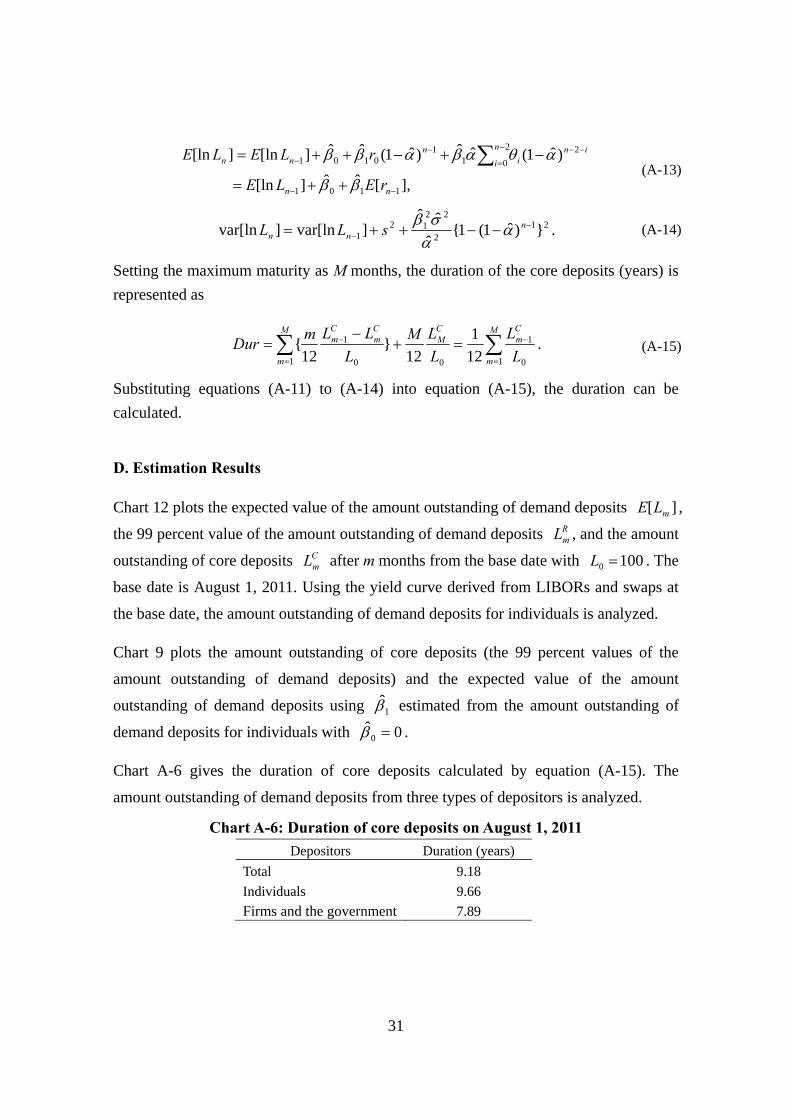
],[ˆˆ][ln
)ˆ1(ˆˆ)ˆ1(ˆˆ][ln][ln
1101
2
0
21
10101
nn
n
i
ini
nnn
rELE
rLELE
(A-13)
212
2212
1 })ˆ1(1{ˆ
ˆˆ]var[ln]var[ln
nnn sLL
. (A-14)
Setting the maximum maturity as M months, the duration of the core deposits (years) is
represented as
M
m
Cm
CM
M
m
Cm
Cm
L
L
L
LM
L
LLmDur
1 0
1
01 0
1
12
1
12}
12{ . (A-15)
Substituting equations (A-11) to (A-14) into equation (A-15), the duration can be
calculated.
D. Estimation Results
Chart 12 plots the expected value of the amount outstanding of demand deposits ][ mLE ,
the 99 percent value of the amount outstanding of demand deposits RmL , and the amount
outstanding of core deposits CmL after m months from the base date with 1000 L . The
base date is August 1, 2011. Using the yield curve derived from LIBORs and swaps at
the base date, the amount outstanding of demand deposits for individuals is analyzed.
Chart 9 plots the amount outstanding of core deposits (the 99 percent values of the
amount outstanding of demand deposits) and the expected value of the amount
outstanding of demand deposits using 1 estimated from the amount outstanding of
demand deposits for individuals with 0ˆ0 .
Chart A-6 gives the duration of core deposits calculated by equation (A-15). The
amount outstanding of demand deposits from three types of depositors is analyzed.
Chart A-6: Duration of core deposits on August 1, 2011
Depositors Duration (years)
Total 9.18
Individuals 9.66
Firms and the government 7.89
32
References
Bank of Japan, Financial System Report, October 2013.
Basel Committee on Banking Supervision, "Principles for the Management and
Supervision of Interest Rate Risk," July 2004.
Black, Fischer, and Piotr Karasinski, "Bond and Option Pricing When Short Rates Are
Lognormal," Financial Analysts Journal, 47 (4), pp. 52–59, 1991.
Cox, John C., Jonathan E. Ingersoll Jr., and Stephen A. Ross, "A Theory of the Term
Structure of Interest Rates," Econometrica, 53 (2), pp. 385–407, 1985.
Financial Services Agency, "Shuyoko muke no sogotekina kantoku shishin, chushou
chiiki kinyukikan muke no sogotekina kantoku shishin, hokengaisha muke no
sogotekina kantoku shishin no ichibu kaisei ni taisuru omona komento oyobi
soreni taisuru kinyucho no kangaekata (Comments on Amendments to
'Comprehensive Guidelines for Major Banks,' 'Comprehensive Guidelines for
Small and Regional Financial Institutions,' and 'Comprehensive Guidelines for
Insurance Companies' and the Financial Services Agency's View)," 2006
(available only in Japanese).
Hull, John, and Alan White, "Pricing Interest-Rate-Derivative Securities," The Review
of Financial Studies, 3 (4), pp. 573–592, 1990.
Ito, Suguru, and Masaaki Kijima, "Ginko kanjo kinri risuku kanri no tameno naibu
moderu (AA-Kijima Model) ni tsuite (An Interest Rate Risk Management
Model for Liability on Banking Accounts: The AA-Kijima Model)," Securities
Analysts Journal, 45 (4), pp. 79–92, The Securities Analysts Association of
Japan, 2007 (available only in Japanese).
Jarrow, Robert A., and Donald R. van Deventer, "The Arbitrage-Free Valuation and
Hedging of Demand Deposits and Credit Card Loans," Journal of Banking &
Finance, 22 (3), pp. 249–272, 1998.
Kamitake, Haruki, and Norio Hibiki, "Ginko no ryudousei yokin zandaka to manki no
suitei moderu (A Model to Estimate the Amount Outstanding and the Maturity
of Demand Deposits in a Bank)," in Japanese Association of Financial
Econometrics and Engineering, ed. Valuation: JAFEE Journal on Financial
Engineering and Econometrics, Asakura Publishing, pp. 196–223, 2011
(available only in Japanese).
Okubo, Yutaka, Yuji Morimoto, Shusuke Kuritani, Masayuki Noguchi, and Takashi
Matsumoto, Zentai saiteki no ginko ALM (Overall Optimal ALM in Banks),
Kinzai Institute for Financial Affairs, 2010 (available only in Japanese).