United StatesDepartment ofAgriculture

NationalAgriculturalStatisticsService

Research Division

SRB Research ReportNumber SRB-93-11

November 1993

SURVEY METHODS FOR BUSINESSES,FARMS, AND INSTITUTIONS

INTERNATIONAL CONFERENCE ONESTABLISHMENT SURVEYS

Part II

NASS Participants

~ .._---,

SURVEY METHODS FOR BUSINESSES, FARMS, AND INSTITUTIONS by Participants,National Agricultural Statistics Service, U.S. Department of Agriculture, Washington, DC20250-2000, November 1993, Part 2 of 2, Report No. SRB-93-11.

ABSTRACT

Part 2 of this report is a compilation of all invited and monograph papers presented at theInternational Conference on Establishment Surveys in Buffalo, New York, June 28-30, 1993.These were requested for the meeting due to there general content regarding NASS policy,program and procedures. These are also ordered by general subject matter. Several of these willbe printed as separate and more detailed research reports. Part 1 of this report included reportsof specific aspects of NASS research.

This paper was prepared for limited distribution to the research community outside theU.S. Department of Agriculture. The views expressed herein are not necessarily those ofNASS or USDA.

ACKNOWLEDGMENTS

This report has been the culmination of the efforts of many individuals in NASS. Special thanksgo to Yolanda Grant and Shawna McClain for their many hours of assistance in preparingfor the conference and this report.

TABLE OF CONTENTS

I. NASS POLICY AND PROCEDURES

Rich AllenThe Evolution of Agricultural Data Collection in the United States 01

Frederic Vogel and Phillip KottMultiple Frame Establishment Surveys 25

Mark PierzchalaEditing Systems and Software 45

Ronald FecsoEvaluation and Control of Measurement Error in Establishment Surveys 61

D. SAMPLING FRMfE AND DESIGN ISSUES

Cynthia Z.F. ClarkEnsuring Quality in U.S. Agricultural List Frames 84

Jeffrey Bush and Carol HouseThe Area Frame: A Sampling Base for Establishment Survey 94

ID. INFORMA TION HANDLING ISSUES

Charles Perry, Jim Burt, and Bill IwigMethods of Selecting Samples in Multiple Surveysto Reduce Respondent Burden 104

IV. NASS PROGRMI COl\fPONENTS

Bob Milton and Doug KlewenoUSDA's Annual Farm Costs and Returns Survey: Improving Data Quality ... 111

George Hanuschak and Mike CraigRemote Sensing Program of the National Agricultural Statistics Service from aManagement Perspective 116

11

THE EVOLUTION OF AGRICULTURAL DATA COLLECTION IN THEUNITED STATES1

Rich Allen2

Deputy Administrator for ProgramsUnited States Department of AgricultureNational Agricultural Statistics Service

Vicki J. Huggins2

Branch ChiefUnited States Census BureauAgriculture Division

Ruth Ann Killion2

Division ChiefUnited States Census BureauStatistical Research Division

INTRODUCTION

Farms represent a special subset of establishments. They, more than any other type ofestablishment, combine business and family considerations. Many farms are operated by asingle person but others involve quite complicated ownership and operation arrangements.Agriculture includes many different forms of products and production practices which oftenchange over time.

This chapter traces the development of agricultural data collection in the United Statesfrom 1790 to the present time. The discussion should be helpful to others for developing orimproving collection of agricultural data. The goal is to summarize major issues anddevelopments. For more detailed reading of historical developments, please see referencesBidwell and Falconer (1925), Brooks (1977), National Agricultural Statistics Service (l989a),Statistical Reponing Service (1969), Taylor and Taylor (1952), and Wright and Hunt (1900).

Major changes in methodology are described with explanations of factors which mighthave allowed or demanded the changes. Methodology for both agriculture censuses and thecurrent agricultural survey programs have changed extensively as the United States evolved

1 The authors have benefitted from several reviews at various stages of the writing and editing process.Reviewers included Doug Miller and Jim Liefer of the Census Bureau; Kenn Inskeep of the EvangelicalLutheran Church in America; Nanjamma Chinnappa and George Andrusiak of Statistics Canada; Bill Arends,Jerry Clampet, Bob Schooley, Paul Bascom, and Lue Yang of the National Agricultural Statistics Service. Theauthors also want to recognize Mary Ann Higgs for her tireless administrative support and Priscilla Simms,Marsha Milburn, and Hazel Beaton for the additional typing and graphics assistance.

2 The views expressed are attributable to the authors and do not necessarily reflect those of the CensusBureau or of the National Agricultural Statistics Service.

from an overwhelmingly rural and agricultural nation to one which is highly urbanized withonly a small fraction of the population involved in agriculture.

Uses of Agricultural Statistics

Early requirements of agricultural statistics in the U.S. stemmed from farmers' need toknow about current and improved farming practices for subsistence reasons. Farmers wereprimarily concerned with increasing production to improve their own family's food and fibersupplies and to purchase goods that they could not produce. Local and state farmingsocieties were interested in farming methods since farming products and practices tended tobe similar by geography. Gradually, the need for national level agricultural statisticsincreased as better marketing channels opened, production expanded westward into newfarming territories, production levels and commercialization increased, and pricingarrangements evolved.

For many years published agricultural statistics were designed largely to providegovernment with production information, and this remains a major purpose. These data areessential for administering farm income support and disaster relief programs and developingnew legislation. Since much agricultural production is exported, current statistics enableorderly marketing in both domestic and foreign trade channels.

Many national and state programs utilize combinations of census and current statistics forallocating funds for extension services, research, and soil conservation projects. Privateindustry uses production data for facility construction and marketing decisions. Purchasersof farm products, suppliers of farm inputs and services, producers, and producerorganizations need good information.

Present Structure of Official Agriculture Data Collection

The agriculture census program of the Census Bureau and the current statistics programof the National Agricultural Statistics Service (NASS)3complement each other quite well.For example, data collected by NASS on prices, production levels, marketing patterns,inventories, and production expenses are used in farm income estimates which are part of theU.S. national accounts. When census data are available, farm income estimation modelcomponents are revised and benchmarked to current census levels.

The Census Bureau is located within the Department of Commerce while NASS is anagency in the Department of Agriculture (USDA). Since the two sets of statistics are createdby different organizations, there is no internal pressure that the census must support what thecurrent statistics have been indicating. There is a good working arrangement andcooperation between NASS and the Agriculture Division of the Census Bureau. NASS aidsin census mail list creation, and its probability area frame survey data are important

3 NASS was previously called the Statistical Reporting Service (SRS). NASS is used throughout this chapterfor consistency.

2

indicators of list coverage. NASS staff assist in reviewing state and county census dataduring the editing phase. The two organizations also participate in joint research projects.

Census Bureau Current Program

Census data collection, currently conducted by the Census Bureau every five years foryears ending in two and seven, represents the only effort to collect a broad set of data fromall farms. Farm operation and family characteristics are collected along with data onacreage, land use, irrigation, crops, vegetables, fruits and nuts, nursery and greenhouseproducts, livestock and poultry, value of sales, type of organization, farm workers, andcharacteristics of operators. The census provides the only set of small area data for farmcharacteristics and minor production items.

The agriculture census is currently a mailoutlmailback enumeration of all farms andranches. Response is mandatory and extensive follow-up procedures are conducted by mail,certified mail, and telephone to improve response rates. Additional data on items such as useof commercial fertilizers; use of chemicals, machinery, and equipment; expenditures; marketvalue of land and buildings; and farm related income are collected from an approximate 30percent sample. A stratified, systematic sample design at the county level is utilized toensure reliable county level statistics.

Following each agriculture census, the Census Bureau has generally conducted one ormore follow-on surveys to collect detailed data on relatively narrow areas of interest withoutadding greatly to overall respondent burden. Past surveys collected information on topicssuch as land ownership, farm expenditures, farm finances, farm and ranch irrigationpractices, and farm energy use. There also have been censuses of horticulture specialties.See Table 3 for a chronological listing.

National Agricultural Statistics Service Current Program

The United States agricultural estimating system for current statistics utilizes voluntarysample surveys to measure production and inventories of major crop and livestock itemsalong with information on prices, labor usage, and disposition of livestock. Expectedproduction levels of major crops are forecasted monthly, starting three or four months beforeharvest. Because many statistics can have an impact on volumes and prices for commodityfutures and cash market trading, strict procedures and laws govern the preparation andrelease of these statistics to the public.

Many different survey vehicles are used, with some programs conducted weekly,monthly, and quarterly in addition to surveys conducted on an annual or semi-annual basis.U.S. and state level estimates are normally produced but county estimates are created foritems needed to administer federal and state farm programs. Most surveys are based onprobability samples but some utilize designated panels of reporters and others are based oncontact of individuals who can answer for an entire segment of a specific population. A fewsurveys contact agribusinesses such as grain elevators, food processors, seed companies,livestock packing houses, and feed companies when they can report data more efficiently

3

than farmers. Administrative data such as exports, imports, and marketings are utilizedeither directly or as a check on estimation levels.

Nearly 400 statistical reports are issued from NASS Headquarters each year on aschedule published before the year starts and more than 9,000 reports are issued by StateStatistical Offices. Six of the current statistics series are included in the Principal EconomicIndicators Series of the U.S. Stalistical Reporting Service (1983)

Farm Dermition

The definition of afann used in the United States has changed over time. The Secretaryof Commerce sets the definition after collaboration and agre.ement with all relevant agencies(Census Bureau, Bureau of Economic Analysis, USDA, etc.) and advisory groups. Thedefinition is not codified in U.S. law. Since 1975, the definition has been any place whichsells, or nonnally would sell, $1,000 or more of agricultural products in the reference year.Because of the relatively low value threshold, individuals who keep just a few head of cattleor sell some fruits and vegetables qualify even if they do not regard themselves as farmers.The greatest difficulty in conducting a complete census or representative survey is inaccounting for the vast number of small farms. In the 1987 census, approximately 50percent of all farms had less than $10,000 in total value of agricultural products sold, 60percent had fewer than 180 acres of land and 30 percent had fewer than 50 acres. Bureau ofthe Census (1989).

Table 1 provides the farm definitions used during different periods of U.S. history.Although defining a farm appears to be a simple task, it requires a tremendous amount ofdiscussion, analysis, and communication to satisfy federal, congressional, and privateconcerns. For example, for the 1974 census, USDA and Commerce both supported raisingthe threshold to $1,000 because of increased prices and changes in the structure ofagricultural operations. However, Congress disagreed and in 1974 census all-farmpreliminary reports were published using the same farm definition as the 1959-1969censuses. Only the final reports were based on the new definition with a threshold of$1,000. Bureau of the Census (1979)

Definition of Counties and Townships

The major geographic administrative subdivision within a state is the county. There areover 3,300 counties within the 50 states of the U.S. Their size varies depending upon thephysical size, geography, and population density of the states. Many counties are dividedinto townships of about 36 square miles each. County and township reports on agriculturewere important at various times in history and counties remain important units for publicationof both census and current agricultural statistics.

4

Table I The U.S. Farm Definition Throughout History

Period(s)

1850-1860

1870-189019001910-1920

1925-19451950-1954

1959-1974

1978-Present

Definition

No acreage requirement, but a minimum of $100 of total value ofagricultural products sold (TVP).A minimum of 3 acres or $500 TVP.Acreage and minimum sales requirements removed.A minimum of 3 acres, with $250 or more TYP or required full-timeservices of at least one person.A minimum of 3 acres, with $250 or more TVP.A minimum of 3 acres or $150 or more TYP. If a place hadsharecroppers or other tenants, land assigned to each was treated as aseparate farm. Land retained and worked by the landlord was considereda separate farm.Any place with 10 acres or more, and with $50 or more TVP, or anyplace with less than 10 acres, but at least $250 TYP. If sales were notreported, average prices were applied to reported estimates of harvestedcrops and livestock produced to arrive at estimated sales values.Any place that had, or normally would have had, $1,000 or more TYP.

AGRICULTURAL STATISTICS BEFORE 1880

In 1790, the United States was essentially an area along the Atlantic Ocean with anaverage width of only 255 miles from the coast and a population of less than four millionpeople, over 90 percent involved with agriculture. Tobacco was the principal agriculturalexport and, valued at $4.4 million, accounted for about 44 percent of total exports. Farmoperations in the northeastern states centered around villages, were often large, multiplefamily plantations in southern states, and were isolated farmsteads in middle states.Economic Research Service (1993)

Before 1840, the only agricultural information available for extensive areas came throughasking knowledgeable individuals for their assessment of current conditions and supplies ofcrops and livestock. An interesting sidelight in American history is that President GeorgeWashington is perhaps responsible for the first agricultural survey. Washington wrote tofriends in several states in 1791 listing agricultural questions that he wanted them to answer.This is the first known occasion when an actual survey form was used to collect expertopinions. Collection of expert opinions was the major source of agricultural statistics for thenext 100 years, except for the agriculture censuses. Statistical Reponing Service (1969)

There were few advances in the collection of agricultural statistics during the first thirdof the 19th century because agriculture was mostly for subsistence. The need for more broadbased collection of agriculture statistics was not apparent. An exception was the South whichwas more commercially oriented and needed information for marketing. Some individual

5

states and agricultural societies collected and provided agricultural information on a smallscale to local farms and businesses.

By the middle of the 19th century, the country was growing rapidly and expandingwestward, agricultural surpluses existed in some areas, and state efforts to collect agriculturalinformation were uncoordinated. The need for national level data became more obvious.

Archibald Russell, a young scholar who prepared a book of proposals for collecting U.S.resource data with the 1840 population census, wrote that an economic understanding of theU.S. could be greatly helped by agricultural data since agriculture was the leading business.In 1838, President Martin Van Buren recommended to Congress that the 1840 Census ofPopulation be expanded to collect information ".. .in relation to mines, agriculture,commerce, manufacturers, and schools ... " As a result, 37 questions about agriculture wereincluded with the 1840 population census. At that time, slightly over 70 percent of the U.S.population reported that they were engaged in agriculture. All information was collected andrecorded by personal interview. The questions concentrated on production without collectingarea harvested or yield which limited comparisons or linking of other information to thecensus. Wright and Hunt (1900)

Table 2 shows the range of questions and the increase in the number of questions relatingto agriculture in the decennial years of 1840 to 1890.

In 1839, the U.S. Congress appropriated $1,000 to the Patent Office for collectingagricultural statistics on new varieties of seeds such as wheat and other agriculturalinformation. It was hoped that providing annual statistics would guard against monopolies orexorbitant prices. The Patent Office issued its first report for 1841 by linking back to the1840 census. Since census estimates of crop areas harvested were not available, estimates ofpopulation change in each state and territory were used as indicators of production changes.Other information came from agricultural societies, agricultural papers, and knowledgeableindividuals.

The Patent Office attempted to track crop failures or other unusual conditions in makingits annual reports. However, in 1849 the Patent Office came under new leadership which didnot support agricultural statistics except for prices and the first continual series of productionestimates ended. Even with an outcry to reinstate the crop reports, no further attempt wasmade to provide annual production estimates. Orange Judd, editor of the AmericanAgriculturist journal, described the Patent Office as a "seed store in Washington." StatisticalReponing Service (1969)

6

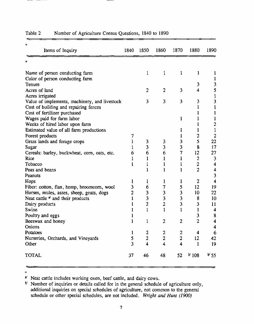
Table 2 Number of Agriculture Census Questions, 1840 to 1890

=Items of Inquiry 1840 1850 1860 1870 1880 1890

=

Name of person conducting farm 1 1 1 1 1Color of person conducting farm 1Tenure 3 3Acres of land 2 2 3 4 5Acres irrigated 1Value of implements, machinery, and livestock 3 3 3 3 3Cost of building and repairing fences 1 1Cost of fertilizer purchased 1 1Wages paid for farm labor 1 1 1Weeks of hired labor upon farm 1 2Estimated value of all farm productions 1 1 1Forest products 7 1 2 2Grass lands and forage crops 1 3 3 3 5 22Sugar 1 3 3 3 8 17Cereals: barley, buckwheat, com, oats, etc. 6 6 6 7 12 27Rice 1 1 1 1 2 3Tobacco 1 1 1 1 2 4Peas and beans 1 1 1 2 4Peanuts 3Hops 1 1 1 1 2 4Fiber: cotton, flax, hemp, broomcorn, wool 3 6 7 5 12 19Horses, mules, asses, sheep, goats, dogs 2 3 3 3 10 22Neat cattle ~ and their products 1 3 3 3 8 10Dairy products 1 2 2 3 3 11Swine 1 1 1 1 1 4Poultry and eggs 1 3 8Beeswax and honey 1 1 2 2 2 4Onions 4Potatoes 1 2 2 2 4 6Nurseries, Orchards, and Vineyards 5 2 2 2 12 42Other 3 4 4 4 1 19

TOTAL 37 46 48 52 !!'108 !!/55

=~ Neat cattle includes working oxen, beef cattle, and dairy cows.!!I Number of inquiries or details called for in the general schedule of agriculture only,

additional inquiries on special schedules of agriculture, not common to the generalschedule or other special schedules, are not included. Wright and Hunt (1900)

7

Because of complaints about many errors found in the 1840 census, the 1850 censusincluded some major changes in organization and data content. Legislation was passed toclearly define the duties of persons employed by the census and the consequences ofneglecting their duties. The general organizational structure initiated in the 1850 census hascontinued through present day censuses. The Census Bureau established a farm definition asany place that had $100 or more in value of sales of agricultural products. A temporarycensus board within the Department of the Interior was established to oversee the conduct ofthe 1850 census, a procedure which was followed until 1900. Wright and Hunt (1900)

By 1860, commercial com and wheat production was well underway with the westdeveloping these crops rapidly. The Northern States began developing other agricultureinterests such as dairying and feed crops. Cotton surpassed tobacco as the major agriculturalexport crop with its $100 million or so average value accounting for half of all export value.Economic Research Service (1993)

There was increased foreign migration into the country as a result of the potato famine inIreland and the German Revolution of 1848 and many immigrants were lured intoagriculture. Scientific invention was applied to create and improve farm machinery. Thenation became increasingly more dependent on national and international markets as it movedfrom subsistence farming toward commercialization. U.S. Census Office (1902)

The average farm size in 1850 was just over 200 acres. However, because of a lawcalled the Homestead Act which made 160 acres of new agricultural land available tosettlers, and the breaking up of southern plantations during the 1860's, the average farm sizedeclined and it was not until 1950 that it again exceeded 200 acres. See Graph 1.

Between 1849 and 1862, when there were no federally collected annual statistics,agricultural societies continued to publish their "interpretations" or estimates. A newCommissioner of Patents in 1856 encouraged governors and other prominent individuals tomake estimates for their areas. However, none of these efforts resulted in a consistentcollection of statistics.

The present day program of current agricultural statistics traces its development to eventsabout 1860. In 1862, Orange Judd asked each town to select a person to fill out a monthlyform on crop area and crop prospects. Respondents were asked to evaluate the currentmonth's data relative to a base of ten as an average crop and to reply in whole numbers, witheach unit above or below ten indicating a 10 percent departure. Mr. Judd received between1,000 and 1,500 responses for various months in 1862. This established the pattern ofmonthly information used by USDA to the present day. Mr. Judd's initiatives and foresightbroke critical ground for ensuring orderly economic commerce of agriculture.

8

Number of U,S, FarmsJ Average and

12

10

8

6

4

2

Total Acreage

Total acreage (hundreds of mi Ilions)

1850 to 198712

10

8

6

4

2

o1B50 1860 1870 1880 1890 1900 1910 1920 '92~ 1930 19]5 19'40 19'4' 1950 19'5~ 1959 196<4 1'969 197.• 1978 1982 1987

o

Mr. Judd's survey was discontinued in 1863 when Congress established USDA whichstarted collection of statistics. This was in response to a grass roots clamor throughout thenation, swelled by the agriculture press, for better data than were being produced by thePatent Office and the decennial census. USDA's first report, using the methods of OrangeJudd, covered estimates for 1859 and 1862 based on 1860 census figures (crop year 1859)and data received on questionnaires sent to every county during the winter of 1862-63.

The Office of the Statistician in USDA was created in 1863 and monthly reports of cropconditions were started immediately. One reporter and five assistants per average sizecounty were selected to provide local agriculture assessments. Reports were sent by mail toWashington, D.C. on a designated day each month. The purpose of monthly crop reportswas espoused by USDA in 1863 as follows: "Ignorance of the state of our crops invariablyleads to speculation, in which oftentimes, the farmer does not obtain just prices, and bywhich the consumer is not benefitted... the true condition of these crops should be madeknown. Such knowledge, while it tends to discourage speculation, gives to commerce amore uniform and consequently, a more healthy action." Statistical Reporting Service (1969)

While the early emphasis was on crop production, cattle, hog, and sheep numbers andvalues were estimated starting on January 1, 1867, along with wheat and com prices for1866. Price data continued to be annual estimates up until 1908 when monthly prices wereinstituted. National Agricultural Statistics Service (1989b)

There was little change in the agricultural data collected in the 1860 and 1870 populationcensuses. There was increased call for information on the acreage of crops such as wheat,barley, and oats, but this information continued to be omitted from the census until 1880.There were some inquiries in the 1860 census relating to "what crops are short," and "usualaverage crop," that may have been useful in crop prediction for intercensal years, but thesequestions were dropped in the 1870 census. The first statistical atlas was published based onthe 1870 results which showed, for example, the geographic distribution of crop production.[See Table 2 for the description of questions in the 1860 and 1870 censuses.]

AGRICULTURAL STATISTICS FROM 1880 TO 1915

By 1880, large cattle operations and wheat production were established on the GreatPlains. Only 50 percent of the population was employed in agriculture but agriculture stillaccounted for over 75 percent of all U.S. exports. Improved tools for production andharvesting had been developed and were in wide use. Economic Research Service (1993)

The census of 1880 marked a turning point in agricultural statistics. Cooperationbetween the census and current statistics programs was at a peak. l.R. Dodge, Chief,Division of Statistics in USDA, served as Chief Statistician for development of the 1880census. He was given considerable freedom in revising the census questionnaire and addedquestions on area harvested and yield. These data were important as a census benchmark aswell as to assist in intercensal predictions. The basic questionnaire had 108 questions aboutagriculture while special schedules contained a total of 1,572 questions. Statistical ReponingService (1969)

10

The 1880 results were presented in both cartographic and tabular forms. The 1880census asked comprehensive questions on renting arrangements and mechanization. Oneother significant feature, which aided interpretation of current statistics surveys, wascollection of information on average and largest cereal crop yields by "region n or "locality."Wright and Hunt (1900)

Periodic reports being issued by USDA were aided by the 1880 census information onacreage and yields and a shift was made to estimates of actual yield at the end of the growingseason. In 1884, reporters were asked to consider 100 as condition of a full crop, not anaverage crop. Another important improvement in procedures was the 1888 initiation of stateweighted averages based on county acreage, since counties varied greatly in area andproduction potential.

Bronsen C. Keller, an economic and social scholar, organized an association with twoother men from St. Louis. These three men had a large impact on the 1890 census bysending a letter in 1889 to people around the country asking them to insist that indebtednessinformation be collected. They believed that indebtedness was leading to loss of farmsthrough foreclosure and hence decreasing ownership. Through this grass roots effort, fivequestions on indebtedness were collected on the population census and the results wereclassified by farm and nonfarm homes.

As agricultural statistics got more attention and the number of users increased, theaccuracy of monthly crop reports began to be questioned. In 1895 the National Board ofTrade passed a resolution stating "Whereas the monthly and yearly crop reports of the U.S.Department of Agriculture have in recent years been confusing, misleading and manifestlyerroneous in important particulars ... that if the crop reporting services... is to becontinued every needful effort be made for ensuring the fullest degree ofefficiency completeness and accuracy of the data... " Taylor and Taylor (1952)

The National Board of Trade established a Committee on Crop Reports which madeseveral proposals for improvement of agricultural statistics. Based on its recommendations alaw was passed by Congress in 1909 making it a crime to divulge any information ahead of ascheduled release. Official township reporting was recommended and, by 1896, there were28,000 township reporters, 9,000-10,000 county reporters, and 6,000-7,000 assistants to statestatistical agents. Reports were also received from 15,000 grain dealers, millers, andelevator operators and 123,000 farmers. Interpreting the vast amount of informationreceived was a difficult task. In 1905, the Crop Reporting Board was established to improveinterpretation. This Board, consisting of state statisticians and experienced headquartersstatisticians assisting the Chief Statistician in reviewing indications and setting estimates, hascontinued for major reports since.

The 1900 agriculture census general schedule was similar to 1890, but added questionson tenure, total value of farm buildings, and ownership of rented farms. Congress providedguidelines for publication which required that data be tabulated by race and gender of farmoperators. There were several processing innovations introduced for this census: punchcards and electronic tabulating machines were adopted and, because of the large number of

11

crop cards, a sorting machine was developed. A new ten-key keypunch machine was usedfor farm census cards 20 years before it was used for the population census.

There were large differences between USDA estimates and the 1900 census results forcrop acreage and production. In almost all instances, USDA estimates were significantlylower than census results. Statistics for the number of acres for two of the nation's largestcrops, com and wheat, differed by 16 percent and 18 percent, respectively. A committee ofinquiry was set up to investigate this and found that the census provided a low base in 1890and that the USDA estimates for subsequent years included accumulated error from faultyyearly percent change ratios applied to the census base. The committee recommendedimprovements in training of census enumerators and clerks, improved editing procedures,and more verification during processing and tabulation of the data. They also recommendedthat a census of population be conducted every five years, especially for the collection ofagricultural information. Statistical Reponing Service (1969)

In 1902, a permanent Bureau of the Census was established in the Interior Department.It was transferred to the new Department of Commerce and Labor in 1903. When thatDepartment split in 1913, the Census Bureau was placed in the Department of Commerce.Establishment of a permanent bureau created a more stable environment for the censusprogram which promoted better planning, comparability between censuses, evaluationopportunities, more time for systems development, and a basis for producing additionalstatistics upon demand.

Specialized censuses on irrigation and on drained land were added to the agricultureprogram. These two censuses remained as part of the program through 1950. Table 3 listsspecial censuses and surveys that have been conducted by the Census Bureau since 1890.Bureau of the Census (1987)

AGRICULTURAL STATISTICS FROM WORLD WAR I TO WORLD WAR II

By 1915, gasoline powered tractors and combines were being developed for theextensively farmed areas. New varieties and disease resistant strains of plants were beingdeveloped. The average value of U.S. agricultural exports was approaching $2 billion ayear, about 45 percent of all exports. Only about 30 percent of the population was nowengaged in agriculture but the need for more commercial agricultural information wasgrowing. There was increased awareness of the importance of marketing and a pressingneed for reliable information on supplies of food and fiber, Economic Research Service(1993)

12

Table 3 Census Bureau Special Censuses and Surveys by Reference Year

II Year Title(s) I Year Title(s) II

1890 Census of Horticulture 1956 Farm Mortgage Indebtedness

1905 Cotton Ginnings ~ 1959 Census of Horticulture,Census of Irrigation,

1910 Census of Irrigation Irrigation in Humid Areas,Census of Drained Land

1920 Census of Irrigation,Census of Drained Land 1964 Survey of Farm Workers,

Survey of Hired Farm Workers,1930 Census of Horticulture, Survey of Farm Indebtedness

Census of Irrigation,Census of Drained Land, 1965 Survey of Nonfarm Income and SourceFarm Mortgage Indebtedness~

1969 Census of Horticulture,1935 Survey of Part-Time Farming, Census of Irrigation,

Farm Mortgage Indebtedness Census of Drained Land

1940 Census of Irrigation, 1970 Agriculture Finance SurveyCensus of Drained Land,Farm Mortgage Indebtedness 1979 Census of Horticulture,

Farm Finance Survey,1945 Farm Mortgage Indebtedness Survey of Farm Energy Use,

Farm and Ranch Irrigation ~1950 Census of Irrigation,

Census of Drained Land, 1984 Farm and Ranch IrrigationCensus of Horticulture,Farm Mortgage Indebtedness 1988 Farm and Ranch Irrigation,

Census of Horticulture,1955 Irrigation in Humid Areas!!1 Agricultural Economics and Land Ownership

Survey

~I The Cotton Ginnings Survey collected data twice a month through the ginnings season every yearfrom 1905 up to the present. The Survey was conducted by the Bureau of Census until 1991;now conducted by National Agricultural Statistics Service.

hI The titles of the Survey of Farm Mortgage Indebtedness, the Survey of Irrigation in HumidAreas, and Farm and Ranch Irrigation Survey have been shortened to better fit the table format.

13

Several important improvements to current agricultural statistics were made between 1910 and1920. Official annual estimates of the numbers of farms by state began in 1910. Monthly conditioninformation was converted to yield forecasts starting in 1911 for crops like wheat, oats, corn, andtobacco. Once the validity of the monthly forecasts was proven, more market volatile crops such ascotton were added. The par procedure was developed to interpret yield by adjusting the ten-yearaverage yield per acre by the ratio of current condition to average condition. As agriculturalstatisticians searched for more mathematically based yield forecasting procedures, regression modelsbased on year-to-year relationships were developed. By 1929, regression models were in commonuse for monthly yield forecasts. Statistical Reporting Service (1969)

An important factor in heightening interest in agricultural statistics was the onset of World War Iin 1917. More information was needed on available food and feed supplies at county, as well as statelevels. By 1920, state and national estimates on 29 crops were being produced, compared to 13 cropsten years earlier, and condition reports were being issued on 44 trOpS - about double that in 1910.Statistical Reporting Service (1969)

The chief of the Bureau of Statistics (USDA) reported in 1919 of the requests for agriculturaldata during World War I that ..A vast amount of information was compiled and furnished in responseto inquiries received by telephone, telegraph, letter, or personal call of representatives of the FoodAdministration, the War Trade Board, the War Industries Board, the Military Intelligence Office ofthe War Department, the Tariff Commission, the Federal Trade Commission, the Council of NationalDefense and other departments of federal and state governments, congress and private individuals ... ".Following the armistice of November 11, 1918, the demand for special agriculture informationdeclined, but demand for food shipment to war torn Europe continued. There was a generalreluctance to discontinue the products and services provided by USDA during the war, so many ofthem continued. Statistical Reporting Services (1969)

Many states developed various statistics programs which meant that different state and federalestimates might be published for the same commodity and respondents might be contacted by multipleorganizations for the same information. Because of the emphasis on more agricultural statisticsduring World War I and respondent burden issues, state and federal organizations in the state ofWisconsin agreed in 1917 to share expenses of data collection and publication. Many states quicklyfollowed suit and today agreements exist in every state involving State Departments of Agriculture orstate agricultural universities or both. These agreements are truly unique within the United States.State funding provides for special publications, surveys, or other services not covered by the federalprogram. All employees (state or federal) work under the NASS selected state statistician whousually has a State Department of Agriculture title and state government duties.

By 1918, to improve reliability of data, sampling was shifted largely from panels reporting fortheir locality to panels reporting for individual farms. This provided a more clearly defined basis forcomparison of production levels. This sampling of farmers in every township became the monthlyFarm Report Survey. Special livestock reporter lists were also established. In 1922, looking formethods to improve livestock statistics, a proposal was adopted to utilize free delivery of mail in ruralareas to provide a broader base of reporters for major reports. Rural mail carriers received a supplyof card type questionnaires to drop off at a sample of farms along mail delivery routes. Completedresponses were forwarded to the state statistician by the Postal Service.

Rural carrier cards collected data for only the current year. Before that time, information wasrequested for both current and past year and a current compared to historic interpretation was made.The main basis for interpretation of rural carrier acreage surveys was calculation of ratios of acreage

14

of specific crops to total cropland or to land in farms. However, ratios were usually biased on thehigh side since progressive farms tended to be sampled and farmers without row crops often did notreport. The approach utilized to adjust for bias was the ratio relative calculation: current year ratioof a crop to total land divided by the previous year's ratio to estimate true change. An effort wasmade by 1928 to look at reports from the same farm on subsequent surveys. Matching providedvaluable information on year-to-year changes, but was extremely time consuming and difficult.

From the beginning, there had been complaints that an agriculture census every ten years was notadequate for an industry with such large fluctuations. Yearly estimates for crop and livestock itemsby USDA relied on the agriculture censuses for a new base or benchmark each ten years.Occasionally, due to the methodologies for projecting yearly changes and any initial bias in censusfigures, annual estimates differed widely from the data for the same year available later in farmcensus findings - for example, the previously described differences observed in 1900. Data usersengaged in agriculture research, farm management, and business investments needed more currentcensus information on agriculture activities. Statistical Reponing Service (1969)

Proposals were floated for annual agriculture censuses or at least a census every five years. In1909, Congress mandated that the Department of Commerce conduct a mid-decade agriculture census.However, because of World War I preparations, the first five-year Census of Agriculture was notconducted until 1925. The five-year census greatly assisted the annual crop and livestock estimatesand provided improved information for decision making.

In addition to providing measures of production, the census of agriculture provides data on theeffects of technological changes on agriculture and on social and economic characteristics of farmoperators. A significant amount of new content was added to the census questionnaire in 1920. Farmoperators were asked if they had gas or electric lighting in their homes and if they owned tractors,automobiles, or trucks. Additional questions in 1930 and 1940 queried farmers about the kinds ofroads adjoining their farms, whether telephones were available, and the presence of new equipmentsuch as combines and milk machines. The presentation of data by type of farm starting in 1930 was avaluable contribution to the analysis of agriculture production. It provided a basis for muchdiscussion and planning on the needs of farms in the early 1930's.

Socioeconomic questions on topics such as hired farm labor, farm versus nonfarm employment,income, race, and tenure of farm operators were asked in all 20th Century censuses. In 1920, forexample, the census found that 61 percent of the rural population and 30 percent of the totalpopulation were engaged in farming. Bureau of the Census (1983)

Other expansions of statistics were made around 1925. The number of crops included onmonthly farm reports nearly doubled. Questions on milk cows and milk production, hens and layerson farms, numbers of eggs produced, and farm labor were added to the monthly farm report. Thepercentage of U.S. farms having various livestock species is shown in Table 4 with comparisons atintervals of about ten years. As percentages of farms with milk cows and chickens declined, thosequestions were removed from the monthly farm report in the 1970's and specific surveys weredeveloped for these data. Bureau of Agricultural Economics (1933)

15

Table 4 Percent of Farms with Livestock, Censuses of 1910 to 1987

Item 1910 1920 1930 1940 1950 1959 1969 1978 1987

All Cattle 83.1 83.1 76.4 79.4 75.5 72.1 63.0 59.6 56.3

Milk Cows 80.8 69.2 70.8 76.2 67.8 48.3 20.8 13.8 9.7

Hogs and Pigs 68.4 75.2 56.2 61.8 56.0 49.8 25.1 19.7 11.7

Chickens 87.7 90.5 85.4 84.5 78.3 58.5 17.3 10.7 6.9

The 1930's brought the next major changes in agricultural estimates. During the periodof extremely dry weather, floods in the South, and critical economic conditions in the U.S.called The Great Depression, there was overproduction of some agricultural products,particularly hogs, resulting in very low prices. Federal farm relief was demanded to helppull the country out of the agricultural slump that began after World War 1.

Many government emergency programs were established to provide financial support tofarmers. One 1933 program called for controlling the supply of hogs by selective destructionof a portion of supply. Thus, good information on supplies was essential. In less than twoyears, 90 additional professional staff members were hired for State Statistical Officesspecifically to develop hog estimates county by county. Brooks (1977)

The 1933 Agricultural Adjustment Act and its successor, the Soil Conservation andDomestic Allotment Act of 1936, were critical milestones in the government's approach toagricultural policy and to the statistical work necessary to support it. USDA was givenunprecedented authority and funds to alleviate distress situations in agriculture. StatisticalReporting Service (1969)

One shortcoming of all procedures used through the 1930's was that up-to-date lists offarms were not available and no other probability sampling frame existed. In 1938, researchto divide the entire land area of the U.S. into sampling units began. The area samplingapproach showed promise and, in 1943, USDA and the Bureau of the Census jointly fundedwork at Iowa State College (now Iowa State University) to create the "master sample ofagriculture." This master sample created segments of land with definite boundaries whichcontained an average of four farms per segment. The master sample was first used tomeasure coverage in the 1945 Agriculture Census.

The use of sampling in the agriculture census was stimulated by World War II to reducecost and time limitations since special statistics were needed during that period. In the 1940Census of Agriculture, data were tabulated separately for large and small farms to identifytheir contribution to production levels and assist in food supply decisions. Sampling as anenumeration methodology was introduced in the 1945 census, when county-level data werecollected through a conventional all-farms canvass, while selected data at various geographiclevels were obtained by sampling. Bureau of the Census (1979)

AGRICULTURAL STATISTICS FROM WORLD WAR II TO TIlE PRESENT TIl\1E

16

The years surrounding World War II saw some of the largest productivity changes inUnited States agriculture. The sad condition of agriculture in the early part of the centurybegan improving. The surplus food problem began to vanish and programs to increaseproduction ensued. Farm production reached a high during the war, despite labor loss anddifficulty in obtaining machinery.

Commercial fertilizer use tripled in a 20-year period, along with continued improvementsin hybrid seeds. Use of irrigation also increased as the country set war time productiongoals. The structure of farms changed as vertical integration -- the ownership of multiplestages of the production, marketing, and distribution functions by one organization -- in thepoultry industry started and new marketing techniques such as frozen foods shiftedproduction patterns. In 1950, only about one-eighth of the labor force was farmers; thiswas down to 2.6 percent by 1990. Agricultural exports are currently about 15 percent of allU.S. export value. Economic Research Service (1993)

After the turn of the 20th Century, data users began requesting information in addition toproduction quantities and sales by product. In determining census of agriculture content, twocontradictory issues had to be balanced: demand by data users for more detailed data and theneed to keep respondent burden to a minimum to encourage adequate response. Experimentsto tailor report forms to reflect different characteristics of farm operations in various regionswere introduced during the 1940's and 1950's. From the 1945 to the 1959 censuses,questions were added to identify emerging farm operational patterns such as landlord-tenantoperations or multiple operations owned by corporations. Technical improvements inprocessing also continued. Mechanical editing of data captured on punch cards began in1940, followed by development of modem computer technology, improved the timing forpublication and controlled the enormous processing responsibilities. The world's firstgeneral-purpose electronic computer, the UNIVAC system, developed to the Census Bureau'sspecifications and installed in 1951, was used for part of the 1950 population census, andthen to process 1954 agriculture census data. Bureau of the Census (1983)

Until 1950, agriculture censuses used personal enumeration--farm to farm canvassing.Drawbacks were delays due to bad weather, smaller pools of census enumerators over time,and difficulty in locating absentee farm operators. For the 1950 census, the Bureauintroduced mail questionnaires with questions phrased as if they were being asked by aninterviewer. Questionnaires were delivered to rural route box holders, who were asked tocomplete the report forms and hold them until an enumerator came. This moderatelysuccessful system was used through the 1964 census.

Throughout history, the agriculture census was taken in conjunction with the decennialcensus, but in 1950, the agriculture program split off and mid-decade censuses were takenindependent of the decennial census. In the 1970's the timing of the census of agriculturewas changed to coincide with all other U.S. economic censuses in years ending in two andseven.

The use of sampling techniques in the census of agriculture program expanded with theintroduction of random samples for follow-on surveys of farms with specific characteristics.Following the 1954 agriculture census, a mail sample survey of farm expenditures was

17

conducted and follow-on surveys such as irrigation and horticultural specialties have beenincluded in every subsequent census of agriculture.

As the use of agricultural statistics grew after World War II, data users requested morecurrent information. Several states had developed cooperative arrangements with theWeather Bureau and with the Federal-State Extension Service to pick up informed opinionson crop progress and fieldwork operations each week to supplement the monthly CropProduction reports. By 1958, this popular "weekly weather crop" approach was expanded toall states with submission of state summaries to NASS headquarters for a national release.

Other than weekly weather crop, the emphasis of agricultural statistics has been ondeveloping probability based methodology to improve the quality and stability of estimatesand forecasts. In 1957, a long range plan for improving USDA agricultural statistics waspresented which called for development of a scientifically distributed area frame sample offarms to strengthen state and national crop and livestock estimates. Since 1964, a JuneEnumerative Survey4 has been conducted in all states except Alaska. This survey, whichyields sampling errors of 1 percent or less for U.S. estimates of major crops, became thebackbone of all improved crop and livestock estimating procedures.

Area frame sampling was extremely successful for crop estimates, but did not providethe same efficiency for livestock numbers because they can vary tremendously (from zero tomany thousands) in relatively small land holdings. One means of stabilizing estimates andsampling errors was creation of lists of large livestock producers who are surveyed withcertainty. Because of the high costs of personal interviewing, the area frame sample is fullyenumerated only once a year in June.

Another livestock survey approach, the probability mail survey, was tried in the mid-1960's. All available information for a livestock species such as hogs was used to create alist sampling frame for that species. Samples were drawn by strata which improved thestability of estimates, since lists were not complete, data expansions did not cover totalproduction and this method was abandoned.

Ongoing internal and external research provided an improved solution in the early 1970'sto livestock estimation difficulties. H.O. Hartley at Texas A&M University developedmultiple frame sampling which utilized the relatively low cost of list sampling with completeuniverse coverage of the area frame survey. Area frame sampling is explored in more detailin Vogel and Kott chapter of this monograph. The June Enumerative Survey was a naturalvehicle for determining completeness of a list frame. Once the base area frame survey hadbeen conducted each year, subsequent mail or telephone surveys would include samples fromthe list frame with supplements derived from the area frame. In addition to livestock, themultiple frame approach was tried for grain stocks, farm labor, production of specialtycrops, and was adapted in the mid-1970's to economic surveys of farm operators. Multipleframe surveys were successful in improving consistency of estimates.

4 Currently called the June Agricultural Survey.

18

The Census Bureau first introduced a mailout/mailback enumeration procedure in the1969 agriculture census. This method of enumeration was more cost effective and allowedfarmers to complete questionnaires at their convenience, permitted unhurried access torecords, and gave respondents a chance to review and correct forms before turning them intothe Bureau. To ensure good response rates, six or seven mail follow-ups, as well astelephone enumeration of large farms, were conducted. Bureau of the Census (1992)

This approach has several problems including development of a complete mailing list andensuring complete and timely response. Identifying small farm operators is especially aproblem since they constantly enter and exit the universe and are not adequately covered byadministrative lists. There is no single list source that identifies all farms. There are sourcessuch as government farm program records, farm tax forms, State Department of Agriculturelivestock inspection lists, etc., which contain farm operator names but also contain names ofindividuals such as landlords who are not farm operators. Some operators do not show upon any list.

Budget efficiencies, as well as the convenience of mailout/mailback, outweigh thedrawbacks. The Census Bureau has evaluated coverage for each census of Agriculture since1945. Net coverage error for number of farms has generally ranged from 85 to 93 percent.And, coverage of agricultural production has consistently been above 95 percent. See theICES Proceedings paper by Clark and Vacca for more information on coverage measures forthe Census and NASS agricultural programs. Despite problems with a mail census, overallcoverage obtained is only marginally lower than personal enumeration conducted prior to1969.

Major list frame development for the agriculture census program began prior to the 1969mailout/mailback census and a major mail list frame development effort began at NASS in1976 to support a mailout/mailback mode of data collection for their current surveys. Theprimary difference between the two mail list programs is that NASS built their mail list oncewith a capability of routine updates and maintenance whereas Census has developed a currentmail list of farm operators for conduct of each upcoming census. Both mail list programsinclude development of computer software routines to convert and standardize name formsfrom multiple lists; matching all portions of names, address, and identifiers across records;prediction of the probability of farm or nonfarm status based on combinations of datasources; and creation of outputs for sampling and list maintenance purposes. The NASS maillist is a source for the census mail list as are Internal Revenue Service farm tax records.

Both agencies constantly strive to improve their mail list by using mathematicalmodelling to improve match success rates and reduce duplication. It is estimated that at least20 percent of active name records on a state's list frame at NASS change in some way eachyear, demonstrating the high volatility in the farm universe.

Emphasis on probability survey techniques had a significant effect on data collectionmethods. Funds were not available for extensive personal interview followup ofnonrespondents so both agencies began using telephone calls for most follow-up in the late1970's. To improve the quality of telephone interviewing, the agencies started researching

19

the use of Computer Assisted Telephone Interviewing (CATI) with interactive editing about1980. See the Werldng and Clayton Chapter for more discussion of CAT!.

Another probability methodology improvement introduced by USDA was development ofprocedures to determine crop yield and production by in-field visits, counts, andobservations. Since the 1960's these objective yield surveys have been conducted for corn,wheat, soybeans, and cotton and procedures have been developed for a wide range of treeand field crops. These surveys depend on forecasting of number of "fruit" (ears of corn,bolls of cotton, number of hazelnuts, etc.) to be present at harvest plus a forecast of weightper fruit. Forecast models utilize historic information for the same time period and maturitystage. Objective yield surveys have been extremely successful but they are expensive sincemonthly on-site visits are required and they are only utilized in major producing states,usually covering 75-80 percent of U.S. production for a given crop.

Since 1972, NASS has utilized aerospace remote sensing as a data source. NASSbecame a leader in the automatic classification of full satellite scenes of digital data involvingmany million pieces of information. The June Enumerative Survey area frame segments arean ideal sample of data for training computer discrimination models and for judging theprecision of classifications. If cloud free imagery can be obtained, classification of thesatellite data after training usually yields sampling errors equivalent to increasing the groundbased sample by three to five times. However, the satellite data can not provide informationfor acreage determination earlier than conventional means. Thus, the value to NASS is forreview of season ending estimates of planted and harvested acreage. Statistical ReponingService (1983).

AGRICULTURAL STATISTICS FOR THE 1990's AND BEYOND

The development of agricultural statistics over the years has provided many innovationsin the field of statistics and data collection. From early concepts such as obtaining reports asvariances from a norm, through design of keypunch and sorting equipment, matching casesfor developing change estimates, the seminal work in area samples at Iowa State University,continuing with research into list frame development, use of questionnaire design techniquesto improve quality of data, use of multiple frame samples and estimation, to being in theforefront with techniques such as interactive editing, the agriculture data collectioncommunity has made many contributions.

The benefits to basic statistical theory and data processing techniques will continue asagriculture data collectors address today's issues. These issues can be divided into threebasic areas: management concerns, technological developments and societal changes. Boththe Census Bureau and NASS, as well as other groups collecting agriculture data, will facethese challenges.

Management concerns include such matters as controlling costs, ensuring appropriatecoverage levels, increasing data quality, and ensuring respondent confidentiality whileproviding maximum data to the users. As U.S. federal budgets become more restrictive,agencies have to determine more cost effective and cost reducing measures while providingincreasingly convincing arguments of the need for data collection in the agriculture sector.

20

As more and more data collection efforts depend on complete list frames, both U.S. agenciesneed to keep abreast of constantly changing operating and marketing arrangements, whilemaintaining substantial evaluation programs to determine the completeness of lists. Theapplication of many federal and state laws depend on accurate agricultural sector data. Bothagencies need to keep a vigilant eye on developments in order to ensure the quality,timeliness, and comparability of data. This includes such efforts as ensuring that customer(legislatures, universities, market researchers, etc.) needs are met.

The confidentiality of respondent data is of utmost importance. The goodwill of datareporters depends on the agencies ensuring that individual data will not be publicly disclosed.The Census Bureau, in particular, is developing an extensive body of theory related to cellsuppression theory which protects respondent data in tabular data presentation. Applicationof the theory can be difficult but is necessary to ensure respondent confidence and, hence,cooperation. The counterbalance to protecting respondent data is providing useful data to themany users. The more data are suppressed to ensure respondent confidentiality, the less dataare available for users. This poses a constant dilemma, since many of the users are payingfor the data collection. See the Larry Cox Chapter on Disclosure as well as the proceedingspapers by Colleen Sullivan and the Panel Discussion on Disclosure. The future holds manypolicy development and statistical innovation challenges.

The area of agricultural technological development is most challenging because it isharder to predict the issues. As technological advances are made in the agriculturalcommunity, such as sustainable agricultural practices, more direct marketing of commoditieslike fruits and vegetables, or growth in the number of farmers producing new crops for veryspecific markets, it is important to gather data about the changes. This is a task made moredifficult by the need to reach some consensus about definitions before attemptingmeasurement.

Technological advances are also occurring in the fields of data collection and statisticalestimation. For example, how will data collection activities change as more and morerespondents use computers and computer driven communications and technology? Datacollectors have an obligation to keep up with -- or, preferably, ahead of -- such trends.

Societal issues run the gamut from maintaining acceptable response rates in a diversesociety to changes in the characteristics of farms as they become larger and more smallfarmers leave the field. Both agencies are currently devoting efforts in the areas ofquestionnaire design, respondent burden, and customer needs. For example, NASS holdsyearly data user meetings around the country, focusing on different types of statistics eachyear, and the Bureau of the Census has increased it's presence at agricultural relatedmeetings. Again, the issue of customer expectations is difficult; meeting the needs of datauser customers while not requiring too much of an ever shrinking community of dataprovider customers is a challenge that will require perseverance and creativity on the part ofboth agencies. The issues of respondent burden may force innovative solutions involvingspecial contacts and wider use of database techniques.

The goal of both U.S. agencies is to be quality oriented in the future. The needs fordata on the agricultural sector will not diminish as the federal, state, local, and private

21

sectors strive to meet their mandates. Planning, research, marketing, and management offarm and rural programs in this country will continue to depend on quality data collectedthrough innovative techniques. Both agencies are determined to meet the challenges of thefuture, as they have in the past!

22

REFERENCES

Bidwell, P.W. and Falconer, J.I., History of Agriculture in the Nonhem U.S., CarnegieInstitution of Washington, 1925.

Brooks, E.M., As We Recall: The Growth of Agricultural Estimates, 1933-1961,Washington, D.C., Statistical Reporting Service, U.S. Department of Agriculture, 1977.

Bureau of Agricultural Economics, The Crop and Livestock Reponing Service of the UnitedStates, Miscellaneous Publication No. 171, Washington, D.C., U.S. Department ofAgriculture, 1933.

Bureau of the Census, 1974 Census of Agriculture Procedural History, Department ofCommerce, Volume 4, Part 4, 1979.

Bureau of the Census, 1978 Census of Agriculture Procedural History, Department ofCommerce, Volume 5, Part 4, 1983.

Bureau of the Census, 1982 Census of Agriculture - History, Department of Commerce,Volume 2, Part 4, 1987.

Bureau of the Census, 1987 Census of Agriculture - History, Department of Commerce,Volume 2, Part 4, 1992.

Bureau of the Census, 1987 Census of Agriculture U.S. Summary and State Data, U.S.Department of Commerce, Volume 1, Part 51, 1989.

Economic Research Service, A History of American Agriculture, 1776-1990, U.S.Department of Agriculture, 1993.

National Agricultural Statistics Service, The History of Survey Methods in Agriculture (1863-1989), U.S. Department of Agriculture, 1989a.

National Agricultural Statistics Service, Agricultural Production and Prices - 125 Years, AHistorical Review, U.S. Department of Agriculture, 1989b.

Statistical Reporting Service, Framework for the Future, Washington, D.C., U.S.Department of Agriculture, 1983.

Statistical Reporting Service, Scope and Methods of the Statistical Reponing Service,Miscellaneous Publication No. 1308, Washington, D.C., U.S. Department of Agriculture,1983.

Statistical Reporting Service, The Story of u.s. Agricultural Estimates, MiscellaneousPublication No. 1088, Washington, D.C., U.S. Department of Agriculture, 1969.

23

Taylor, H.C. and Taylor, A.D., The Story of Agricultural Economics in the United States,1840-1932, The Iowa State College Press, Ames, Iowa, 1952.

U.S. Census Office, Census Repons: Twelfth Census ofthl' U.S.: Farms, Livestock, andAnimal Products, U.S. Government Printing Office: Washington, D.C., Volume V, Part 1,1902.

Wright, C.D. and Hunt, W.C., History and Growth of the U.S. Census: 1790-1890, U.S.Government Printing Office, 1900.

24

MULTIPLE FRAME ESTABLISHMENT SURVEYS

Frederic A. VogelNational Agricultural Statistics Service

Phillip S. KottNational Agricultural Statistics Service

1 INTRODUCTION

Sample surveys of economic establishments are usually designed to provide estimatesof characteristics such as total sales, expenditures, number of workers, and inventories for apopulation of interest. Basic principles from finite population sampling theory applyregardless of the specific sampling design used. A population of elements must be defined(not always a trivial task in establishment surveys, see Colledge chapter and Nijhownechapter), and a sampling frame must be constructed from which a sample of elements canultimately be drawn. Every element in the population must have a known probability ofselection. Ideally, the frame should also be complete; that is, the selection probability ofevery element in the population should be positive.

The general term "element" is used to mean a statistical unit in the sense of theColledge and Nijhowne chapters. In many establishment surveys, but certainly not all (seeSubsection 3.1), the population of elements is identical to the population of establishments ofinterest.

Populations of establishments, whether of farms, retail stores, factories, buildings,schools, or governments often possess common characteristics that impact on the choice ofsampling frame and overall sample design. Among these characteristics are skeweddistributions, diversity of variables of interest, and changing population membership.

Because establishment populations are skew, efficient sample designs for their surveysdemand the use of list frames that incorporate known or projected measures of size for eachelement in the population (see Sigman and Monsour chapter). Unfortunately, when thevariables of interest are diverse and weakly correlated, a single list frame with one measureof size will not suffice. Moreover, the changing nature of the population causes any listframe or combination of list frames to become outdated quickly and therefore incomplete interms of coverage of the population.

One way to assure the completeness of the frame is to use an area frame covering theentire population of interest so that all the elements in the population and all potential futureelements will be located somewhere within the area frame. Whereas a list frame is a list ofthe elements in the population, an area frame is a collection of geographical units or areasegments. In list frame designs for establishment surveys, the sampling units are usually the

25

establishments themselves, and stratified single stage sample designs are commonly used toselect establishments directly from the list. In area frame designs, area segments are thesampling units, and these units are often selected using stratified multistage designs.Correspondence rules are needed to link the establishment in the population to the areasegments in the frame in a unique manner.

Although area frames ensure complete coverage, they do not generally lead toefficient sampling designs because area segments are essentially clusters of elements.Segment sizes (in terms of numbers of constituent elements) are usually unequal andunknown at the time of the sample design. In fact, there is no guarantee that an areasegment contains any establishments at all. Large area sample sizes will be needed toovercome problems with populations containing rare items (variables) and with skeweddistributions.

Area frames are most useful for general purpose surveys covering a wide spectrum ofitems that are fairly evenly distributed geographically or when the sizes (as defined above) ofthe area segments are available or can be estimated reasonably well. That is why they areused so often in demographic surveys where population censuses provide adequate measuresof the size of an area segment. It should also be noted that an area frame has a long lifespan. It only needs to be updated when geographic features have changed to the point that itbecomes difficult to associate population elements with sampled area segments or when theavailability of more up-to-date information allows for the development of improved samplingdesigns. This occurs often in agricultural surveys with the use of recent aerial photographsand/or satellite data.

Area frame establishment surveys are generally more expensive than list framesurveys of comparable sample size. This is because area frames are usually much morecostly to develop. In addition, sampled establishments from an area frame often have to bepersonally enumerated, while sampled elements from a list frame can be enumerated bytelephone or electronically.

A multiple frame survey uses a combination of frames. The primary reason for usingmultiple frame sampling for establishment surveys is to utilize the strengths of one frame tooffset the weaknesses of the other. In principle, the theory of multiple frame sampling canbe applied to the use of more than one list frame (see, for example, Bankier 1986). Themain focus here, however, will be on combining the use of list and area sampling frames.Area frame sampling assures completeness, while list frame sampling can be designedefficiently for large and rare items.

Section 2 outlines the theory of sampling from multiple frames. Section 3 discussesthe most common use of multiple frame sampling in which there is a single list and a singlearea frame. Section 4 addresses subsampling from an area frame. Section 5 reviews somepractical problems with overlapping frames. Section 6 briefly discusses future directions inmultiple frame methodology.

26

2 FUNDAMENTALS OF MULTIPLE FRAME SAMPLING

This section develops some theory for sampling and estimation from multiple frames.Each frame consists of a set of mutually exclusive primary sampling units, and there exists aone-to-one or many-to-one mapping from the elements in the population of interest to theprimary sampling units in a particular frame. The mapping need not be complete for eachframe (i.e., some population elements may not be associated with any sampling unit for aparticular frame). For simplicity, we will speak of an element belonging to a frame when itmaps onto a sampling unit in the frame (sometimes these elements are referred to as theultimate sampling units of the sampling frame). After one or more stages or phases ofrandom sampling, a sample of elements is drawn independently from each frame.

Two important assumptions are made in this section. They are:

Completeness - Every element in the population of interest must belong to at least oneframe; and

Identifiability - It should be possible to determine whether or not a sampled elementfrom one frame belongs to any other frame and hence could also have been sampledfrom it.

The completeness assumption is satisfied whenever an area sampling frame covering theentire population of interest is one of the multiple frames. The identifiability assumption,while simple in theory, poses most of the operational difficulties in implementing a multipleframe survey. This is because it is not always a trivial matter to ascertain whether anelement sampled from one frame is also contained in another frame (see Section 5).

The basic theory of multiple frame sampling was developed by Hartley (1962) andextended by Cochran (1965). Hartley divided the population into mutually exclusive domainsdefined by the sampling frames and their intersections. For example, if there are twosampling frames, A and B, there are three possible domains:

Domain (a) containing elements belonging only to Frame A;

Domain (b) containing elements belonging only to Frame B; and

Domain (ab) containing elements belonging to both Frames A and B.

With k frames, there will be 2k. - 1 domains (recall the completeness assumption precludesthe existence of a domain without any members from at least one frame).

27

Let us focus attention on the two frame example introduced above to clarify some ofthe issues involved in estimation using multiple frames. Suppose we are interested inestimating a population total T. It is possible to decompose T as

(1)where Td is the population total in domain d (d = a, b, or ab). Attention in this chapter willbe principally focused on estimating population totals. Extensions to other populationparameters are briefly discussed in 3.3.

When d = a or b, one can estimate Tdwith the Horvitz-Thompson expansionestimator,

td = E ejYi,i€Sd

(2)

where Sd is the set of sampled elements in domain d, ei is the expansion factor (the inverse ofthe selection probability), and Yi is the item value of interest for element i. This estimator isunbiased under the sampling design.

A continuum of unbiased estimators for Tab is given by

tab(Pl = p E ejYj + (1 - p) E ejYii€Sab

Ai€Sab

B

= (3)

where 0 < p ~ 1, Sab G is the set of elements in domain ah sampled from frame G(G = A or B), and tab G is the Horvitz-Thompson estimator for Tab based on the frame Gsample. The limits on p assure that tab(p) will be non-negative whenever the Yi arenon-negative.

We now have a continuum of unbiased estimators for T:

(4)

where 0 < p ~ 1. The sampling design is independent across frames but not necessarilyacross domains. Consequently, The variance of tp is

Var(t(p» = Var(ta) + Var(tb) + 2pCov(ta, tabA)

+ 2 (1 - p) Cov (tb, tabB)

+ p2Var(tabA) + (l-p)2Var(tab

B).

28

(5)

It is reasonable to choose p so that the variance of t(p) is minimized. The optimal(i.e., variance minimizing) p is

Var(tabB) - Cov(t., tabA) + Cov(tb, tabB)

p =Var(tabB) + Var(tabA)

If the two co-variance terms in (6) were zero (or equal to each other), p would take on

the form:

(6)

p =Var (tabB)

var(tabB) + Var(tabA)I (7)

which always lies between zero and one. As one would expect, the size of p is directlyrelated to the precision of tal/ relative to that of tab

B• The more relatively precise the FrameA sample is in estimating domain ab, the more weight tab

A is given in the estimation of Tab.

The expansion factors, ej, in the above expressions can be either unconditional orconditional. That is to say, they may reflect either the original probabilities of selection orthe recomputed selection probabilities within the domains. For example, if the sample designin Frame A were simple random sampling without replacement, then the unconditionalexpansion factor for every sampled element from the frame would be NAlnA, where NA and nA

are the respective sizes of the population and sample in Frame A, while the conditionalexpansion factors for the sampled elements in the intersection of domain d and Frame Awould be NA(d/nA(d), where NA(d) and nArd) are the respective sizes of the population and samplein this intersection.

There are theoretical reasons for preferring estimation with conditional rather thanunconditional expansion factors (see Rao 1985). In many applications, however, especiallythose involving an area frame (where population sizes are often unknown), conditionalselection probabilities will be either impossible to calculate or impractical. Consequently,unconditional inference will have to suffice.

Although one can, in principle, choose p so that the variance (conditional orunconditional) is minimized, this is usually impossible to do in practice because thecomponent variance and co-variance terms in equation (5) are unknown. They could beestimated from the sample, but then the choice of p would not really minimize the varianceof t(p) but the estimated variance of t(p). As a consequence, this estimated variance would bebiased downward.

Even if the distinction between the variance-minimizing p and the estimated variance-minimizing p could be ignored, the following inconvenience remains: the optimal p can varyfrom survey item to survey item. This point as demonstrated by Armstrong (1979) withCanadian farm data.

A popular alternative is to eschew issues of optimality or near optimality and fix the

29

value of p in advance, most commonly at zero. One can then estimate the components onthe right hand side of equation (5) in an unbiased fashion and create an unbiased estimatorfor the variance of t(p). This approach would be biased if p were estimated from current datainstead of being fixed, because the estimated variance of t(pi is no longer a linear combinationof unbiased estimators.

It is possible to develop a more direct Horvitz-Thompson estimator for T in equation(1) by treating the samples from the two frames as a single sample and then computing theprobability of selection for each sampled element (the sum of its probability of selection fromeach frame minus the product of these two terms). There is no reason to believe, however,that the resultant estimator will have less variance than t(p) when a near optimal p is used.Moreover, estimating the variance of this alternative will often be quite difficult.

Finally, one can sometimes improve on t(p) by using auxiliary information. Theinterested reader is directed to Fuller and Burnmeister (1972), Bosecker and Ford (1976),Bankier (1986), Skinner (1991), and Rao and Skinner (1993).

3 THE DOMINANT SPECIAL CASE: ONE LIST FRAME, ONE AREA FRAME

The U.S. Census Bureau's 1949 Sample Survey of Retail Stores (Hansen et aI. 1953)was one of the first establishment surveys that used a multiple frame technique. It employeda single list frame and a single area frame. This two frame approach is still used in theBureau's Monthly Retail Trade Survey. Nevertheless, it is fair to say that the approachcurrently finds its widest use in surveys of agriculture. See Vogel (1975) and Julien andMaranda (1990) for respective discussions of U.S. and Canadian multiple frame agriculturalsurveys.

3.1 Area Sampling

The subject of list sampling for establishment surveys has been reviewed in somedetail in the Sigman and Monsour chapter. Area sampling concepts for establishmentsurveys require some additional discussion.

The basic concepts of area frame sampling are simple. The total area to be surveyedis first stratified by geography or other known characteristics that are related to the variablesof interest (population density is one such characteristic for a retail survey, farm density isone for an agriculture survey). A sample of segments -- usually compact blocks of land -- isthen selected within each stratum, perhaps using a multistage sampling design.

Gallego and Delince (1993) discuss sampling designs where points are randomlyselected within sampled area segments. In this section, however, we focus on designs forwhich the last stage of sampling is the selections of area segments. When employing suchdesigns, rules need to be developed to uniquely link (map) the elements in the populationwith the sampled segments. The area expansion factor for each element is simply the inverseof the selection probability of the segment with which it is linked.

30

Although the basic concepts are simple, the successful application of area framesampling can become very complex, especially if used in a multiple frame environment. Thetheory and application of area frame sampling are well documented and include Jessen(1942), King and Jessen (1945), Houseman (1975), Nealon and Cotter (1987), and Bush andHouse (1993). Fecso et al. (1986) contains a good list of references covering area framesample design issues.

The link between population elements and sampled segments is complicated in thosearea frame surveys (e.g., agricultural surveys) where the physical location of establishments(farms) may cross segment boundaries. There are three approaches to redefining theelements of an area frame frequently used in this situation.

In the closed (or tract) approach, an element is defined as the intersection of anestablishment and an area segment (Le., the portion of the establishment that lies within thearea segment). Response errors occur when the reporting unit, usually the establishment, isnot able to measure and report on that portion of its business that lies within the selectedsegment's boundaries.

The closed approach is statistically robust and relatively efficient for items that aregenerally distributed evenly over wide areas, such as crop acreages. Outliers can becontrolled by the size of the segment for many of these items. For example, if the segmentsize is 600 acres, the maximum acres for any crop in the segment is 600 acres even though asingle establishment located in the segment may account for many times that number of cropacres in its entire operation.

In the open approach, an element is defined to be an establishment and is linked onlywith that segment containing its headquarters. This can lead to difficulties with largeestablishments with complicated corporate or partnership structures. For example, manymedical practices involve several doctors with offices in more than one location andidentifying the "headquarters" may not be simple. Complex counting rules must be devisedthat ensure such establishments do not have a chance of being linked with more than a singlearea segment.

A sampled segment will likely contain fewer elements with larger item values whenusing the open approach to defining elements as opposed to a closed approach. As a result,the former is often less statistically efficient than the alternative. A potential advantage ofthe open approach, however, is that once the establishment has been defined, it may beeasier for the respondent to report values for the entire establishment rather than for thatportion of the establishment located within an area segment. Segment boundaries will havelittle intrinsic meaning to many respondents.

In theory, the definition of the element in the weighted approach is the same as in theclosed approach: the portion of an establishment that lies within an area segment. Thedifference is in the data values attributed to the element. Data values for an establishmentthat is the "parent" of several elements (each in a different area segment) are prorated usingfixed weights defined so that they sum to unity. For agricultural surveys, it is common to

31

use the fraction of the establishment's (farm's) land within a sampled segment as the weightfor the element in that segment.

The weighted approach leads to less sampling variability than the open approachbecause large operations are spread across many segments. One major problem with thisapproach, especially when it is applied to agricultural surveys, is that the weights themselvesare prone to measurement errors (see Nealon 1984, p. 19).. In principle, the weights for allthe elements with the same parent establishment should sum to unity. In practice, since onlyone of these elements is likely to be selected in an area sample, pains must be taken to assurethat the weight used to prorate establishment values to sampled elements are notsystematically larger or smaller than they should be.

Nealon (1984) provides a theoretical and empirical examination of these threeapproaches for area frame and multiple frame surveys conducted by the U. S' s NationalAgricultural Statistics Service (NASS). The results favor the weighted approach. Houseman(1975) contains a more in depth discussion of the three approaches. Faulkenberry andGaroui (1991) explore additional approaches.

3.2 Estimation

Suppose two frames are to be used, one list and one area frame, and a total is to beestimated. Using the notation of Section 2, let A denote the area frame and B the list frame.Observe that domain b is empty because all elements should be located somewhere on thearea frame. Consequently, Tb = tb = O.

In almost all applications of the two frame design, p in equations (3) and (4) is setequal to zero, rendering t = ta + tal. This value for p, besides being convenient forvariance estimation purposes, is often close to optimal (depending on the efficiency of the listframe stratification) because the variance of the list frame estimator of domain ab (i.e., tu,~is almost always considerably smaller than the variance of the area frame estimator of thisdomain (ta/) (recall Section 1). Consequently, equation (7) suggests that p should be verysmall. Depending on the content of the list frame, Cov(ta, ta/) in equation (6) may actuallybe positive because ta and tab

A are based on the same sampled segments. This would makethe optimal p even smaller (note: Cov(tb, tabB) in (6) must be zero because tb is always zero).

A little renaming to simplify the notation: let tL = tab(O) = tabB, since it is the Horvitz-Thompson expansion from the list frame of domain ab (the overlap domain); and lettN = ta, since it is the area expansion for the nonoverlap domain (using either the closed,open, or weighted approach to element definition).

The estimator for the total, t = tL + tN' is called the screening multiple frameestimator because elements in the area sample are "screened" and only those in thenonoverlap domain are enumerated. Its variance has the obvious form:

(8)

32

Estimating Var(tJ is straightforward when, as is usually the case, tL is based on a singlestage stratified list sample. Estimating Var(tN), however, can be a bit more complicated.Recall that a sample of segments was selected from the area frame. In many cases thedesign used is roughly equivalent to stratified simple random sampling (see Kott 1989). Inpractice, sampling fractions are so low within strata that the distinction between with andwithout replacement sampling can be ignored. Suppose there are H strata and nh sampledsegments within stratum h. If XIg is the sum of the expanded values of all nonoverlapelements in segment j of stratum h (i. e., eh E Yj, where eh is the expansion factor for allsampled elements in the stratum h, Yi is the value of element i, and the summation is over allnonoverlap elements in segment)), then

H nh nhvar (tN) = E nh/ (nh - 1) { E Xh/ - [ E Xhj] 2/nh}

h=1 j=1 j=l(9)

is an unbiased estimator for Var(tN) whenever finite population correction can be ignored.Although equation (9) appears straightforward, one needs to be aware that XIg will be zerofor many sampled segments either because there are no elements linked with the segment orbecause the elements linked with the segment are also on the list frame.

3.3 Estimating Means, Ratios, and Regression Coefficients

The area sample is composed of elements, while the population itself is composed ofestablishments. Although this difference poses no problems when the goal is estimatingpopulation totals, it can when estimating population ratios -- which include population means-- and regression coefficients.

Estimating population ratios and regression coefficients with a multiple frame sampleis a relatively trivial matter when the open approach to element definition in the area frame isused (and, as in the last subsection, p = 0). When an establishment selected from the areaframe is in the overlap domain, the establishment's area frame data values are ignored inboth the numerator and denominator of a ratio estimator. An analogous technique is used forestimating population regression coefficients. As in equation (9), however, estimates ofvariance need to reflect the existence of those sampled segments that do not contribute to theestimation of the parameter itself.

When the weighted or closed approach is used, estimating ratios is againstraightforward since either approach can be used to estimate the appropriate total in both thenumerator and the denominator. It is unclear, however, how one can estimate populationregression coefficients with the closed approach. The weighted approach is discussed below.

33

A finite population regression coefficient has the form:

B = ( E Xk'Xk) -I E Xk'Yk'kEP kEP

where

k denotes an establishment,P denotes the population of establishments,Yt is a value attached to establishment k, andXt is a row vector of values attached to k.

(10)

Without loss of generality, we will assume that the elements of the list frame sampleare, in fact, establishments. In what follows, an establishment is said to be "associated" witha sampled element when it is sampled from the list frame or when it is the parent of asampled element from the area frame.

A reasonable estimator for B that uses the weighted approach to element definition is

where

b = ( E ekwkdkxk' Xk)"1 E ekwkd.:xk' Yk ,kES kES

(11)

S is set of establishments associated with sampled elements,el; is the expansion factor for the element associated with k,WI; is the weight attributed to the element associated with k if is sampled from the area

frame, one otherwise, anddl; is 0 if k is associated with an element sampled from the area frame that is also on the

list frame, one otherwise.

Two observations about equation (11) are in order. One, the set S may, in principle,include particular establishments more than once due either to list/area overlap or to aparticular establishment being in two sampled area segments. The die and Wle terms assure usthat neither the y-values nor the x-values for such establishments will be double-counted.

Two, if we call gt = etwt!ile the adjusted expansion factor, then b can be expressed asb = (Eko;sgtXt'XJ-1 Eko;sgtX/YIe. In this form, one can use a survey analysis software packagelike SUDAAN (Shah et al. 1991) to calculate b and estimate its variance.

4 SUBSAMPLING FROM AN AREA FRAME

In this section, we explore two methods of subsampling from an area frame sample.What distinguishes these methods from simple multistage area sampling is that eachincorporates the development of a list frame for subsampling.

34

In the method described in 4.1, one starts with an area sample of primary samplingunits (PSU) and then uses a multiple frame estimation strategy (list and area) within eachPSU. In the second method described in 4.2, one starts with an area sample of elementsusing the weighted method of element definition and then draws a subsample of theseelements. Since it is not required that subsampling be done independently within the originalsampling units, this is a two-phase sampling design (see Sfundal et al. 1991, Chapter 9).

4.1 Using Multiple Frame Designs Within Area PSU's

There are many situations where the cost of developing a list frame is prohibitivelyhigh. On the other hand, the variance of an estimator based on a pure area frame sample isprone to be unacceptably large.

This was the situation faced by the designers of the U.S. Commercial BuildingsEnergy Consumption Survey (CBECS) which measures the consumption of energy incommercial buildings (Energy Information Administration 1989). Their solution was to use amulti-stage area sample and to create list frames of large commercial buildings withinsampled PSU's. This approach reduced the potential size of the expansion factors for suchbuildings.

Let j denote a PSU, and Tj the first stage expanded values of interest from allelements in the PSU. A list and area multiple frame estimation strategy can be constructedto estimate each Tj. Since the elements in the CBECS were buildings that never crossedsegment boundaries, the linking of elements to the area segments was straightforward.

The estimator developed for the CBECS survey did not estimate each Tj with amember of the family in equation (4). Instead, the CBECS estimator has a form equivalent to

t/ = tj + e 1j ( 1;k€P/

(12)

wheretj is the screening estimator (~L + tjN) for Tj,eIj is the first stage (PSU) expansion factor,lj' is the set of all elements subsampled from the area frame that are also on the listframe in PSU j,~' is the set of all elements subsampled on both the list and area frames of PSU j, and

eu; is the inverse of the probability that element k is subsampled from the list frameinj.lt is not difficult to show that ~' is unbiased (Chu 1987).

Let dy = ~' -~. The variance of tj' conditioned on the first stage selection of PSU j is

(13)

where the subscript 2 denotes the conditional nature of the variance (co-variance) operator.Since the co-variance term in equation (13) is likely to be negative, it is possible for ~' tohave less variance that tj•

35

Now consider unbiased estimators having the general form:

where c is a constant. Observe that tjc = tj when c = 0, and tjc = tj' when c = 1. The valueof c may be chosen so that the variance of tjc is minimized" although that may not be easy todo in practice.

Suppose there are H strata in the original area frame and nh sampled PSU's withinstratum h. A variance estimator for tc = Lh Lj tjc is

H nb nh

var(tc) = L nh/(nh-1) { L tjc2 - [ E tjc]2/nh}.

h=l j=l h=l(14)

This estimator is unbiased when the first stage sample is drawn with replacement and isnearly unbiased in many practical applications when PSU's. are selected without replacement.Goldberg and Gargiullo (1988) discuss variance estimation for surveys (like the CBECS) inwhich some PSU's are selected with certainty.

4.2 Using Lists Across Area Segments

Suppose one has previously drawn a sample of segments from an area frame for aparticular multiple frame (list and area) survey and now wishes to mount a new, smallersurvey to estimate different population parameters. This happens frequently in agriculturalsurveys where different parameters are of interest at different times of the year and particularparameters may change over time. Suppose further that the same list frame will beemployed for the new survey so that the nonoverlap domain is effectively fixed. Althoughthis supposition is not necessary, it greatly simplifies the exposition.

In order to reduce the sample size for the new survey, the elements of the area framesample can be subsampled. Since list sampling is generally more efficient than areasampling, it makes sense to use list sampling techniques to draw such a subsample.

Elements sampled from the area frame can be separated into two groups: those thatoverlap with the list frame and those that do not. As discussed in 3.2, the values of overlapelements are ignored when estimating T with the screening estimator,t = tL + IN. This means that these elements are attributed values of O. Since we know theirvalues in advance of subsampling, we can think of any subsample as containing all originallysampled overlap elements (these elements do, however, need to be in the original sample sothat we can determine whether or not they are in the overlap domain). The only questionthen is how to subsample from the sampled nonoverlap elements.

Let e Ii be the original expansion factor of element i from the area sample, Wi be theweight attributed to i in the weighted approach to element definition. In the open approach,

36

Wj is unity. Let Yj be the value of interest for the establishment associated with i. Define~ = eliwYj. The goal of subsampling from the area frame sample is to estimate

t ' -N - (15)

where NA is the set of nonoverlap elements in the original area sample. In the openapproach, NA is restricted to elements with headquarters in the original area sample.

List sampling designs to estimates parameters like tN' in equation (15) in an unbiasedand efficient manner are the subject of the Sigman and Monsour chapter. There is norequirement that the original area sampling design be reflected at all in the subsamplingdesign used to estimate tN'. At the U.S. Department of Agriculture, for example, areasampled nonoverlap elements from the large June Agriculture Survey are restratified for"follow-on" surveys in subsequent months. Those elements believed to have similar ~ valuesare placed in the same subsampling stratum irrespective of their original area stratum or theiroriginal expansion factor (except so far as eli impacts on z), and a without replacementsimple random sample is drawn within each new stratum.

An attractive alternative to stratified simple random sampling is probabilityproportional to size (Pps) sampling, which can also incorporate stratification. Since there arelikely to be a number or values of interest in the new survey and because Yj values areunknown before enumeration anyway, one may choose to treat the eliwj as the measures ofsize for pps sampling. Alternatively, data from the original survey can be used to determinereasonable measures of size.

A Horvitz-Thompson expansion estimator for tN" and thus TN' is

tN = E e2izj

i€N2

(16)

whereez; is the inverse of element i's probability of being subsampled given it is in the originalarea sample,Nz is the set of elements subsampled from the nonoverlap domain of the area frame, andgj = e2leliwj•

It is interesting to note than when unstratified probability proportional to eliwj sampling isused in the subsampling, gj is identical for all subsampled elements.

The variance of the two phase estimator described above is the sum of the variance oftN' in equation (15) as an estimator of TN (which was discussed last section) plus the expectedvalue of the variance of tN in equation (17) as an estimator for tN' (Cochran 1978). Anestimator for this variance is more difficult to express. Sfundal and Swensson (1987) providea general formulation.

37

Kott (1990) explores the important special case where the first phase is a stratifiedsimple random sample of area segments and the second phase is a (re)stratified simplerandom sampling of elements, It turns out that if xhj is the sum of the fully expanded valuesof all nonoverlap elements in area segment j of stratum h and there are nh sampled segmentsin stratum h (h = 1, ,." H), then

H nb nbvar (tN) = E nh/ (nh - 1) { E Xb/ - [ E Xbj] 2/nh} ,

h=l j=l j=lis biased upward as an estimator for the variance of (N'

(17)

It is well known that equation (17) is unbiased under two-stage sampling when thefirst stage sampling fractions can be ignored. This is because the xhj are (virtually)independent. In the design discussed in Kott (1990), the xhj tend to be inversely correlated:when one segment has more elements than expected -- and thus a larger xhj value -- anothersegment would tend to have fewer elements than expected. Such inverse correlations tend todepress the variance of ( = EH Ejxly' while increasing the value of the right hand side ofequation (17). This informal reasoning suggests that equation (17) is likely to provide aconservative variance estimator for two phase estimation strategies more complicated than theone formally treated in Kott (1990).

5 PROBLEMS IN SURVEYS WITH OVERLAPPING FRAMES

As noted in previous sections, an area frame provides complete coverage of thepopulation, but it can lead to inefficient estimation when the population of interest has askewed distribution. A list frame, by contrast, can provide the means for more efficientestimation, but is often incomplete.

When a list of establishments is used along with an area frame in a multiple frameenvironment, the list need not be complete. It should, however, contain those large and rareestablishments which are the bane of area frame surveys.

5.1 List Frame Issues

All establishments on a list frame must be completely identified by name, address,etc. Operations that are large, have complex management structures, and/or are scatteredover different locations must be so identified. This is the identifiability assumption describedin Section 2. In a two frame (list and area) sampling design one must be able to determinewhether an establishment (or portion of an establishment) sampled from the area frame couldalso have been selected from the list frame; otherwise, intractable nonsampling errors willresult. It must be realized, however, that the identifiability requirement can greatly increasethe cost of list development.

When developing a list frame of establishments, more than one source of

38

establishment names are often available. The survey designer must decide whether to useeach list as a separate frame in a multiple frame surveyor to combine the lists prior tosampling and create a single list frame for sampling purposes.

Suppose the former approach is chosen with two list frames and a single area frame.The population can then be divided into four mutually exclusive domains: (1) establishmenton neither list frame, (2) establishments on the first list frame but not the second, (3)establishments on the second list frame but not the first, and (4) establishments on both listframes.

One can see that the need to identify all domains when there are two or more listframes greatly complicates the survey and estimation process. Many statistical agencies havetherefore decided that it is usually more practical to combine all lists and remove duplicationprior to sampling. This can still be a significant undertaking requiring the use of recordlinkage methodologies that may be prone to errors. These methodologies are discussed inthe Winkler chapter.

5.2 Overlap Detection Issues

The reliance upon matching names on the list frame to sampled elements from thearea frame to determine overlap complicates the survey process. Whether an establishmentis surveyed via the list or area frame, it is necessary to determine the primary business name,other business names, and the names of individuals who are also associated with thebusiness. Rules of association of individuals' names with establishments must be defined.For example, an area frame unit may contain the residence of Dr. X associated with themedical practice of Drs. X, Y, and Z. Should the association of the establishment with anarea frame element be based on the residence of each name or on the location of the businessitself} This will depend upon the counting rules used to determine the overlap between theframes. This example becomes more complicated if there is a Dr. T involved in the practice,but the list frame only identifies the practice involving Drs. X, Y, and Z. If counting rulesare used that would allow Dr. T to report for the entire practice of Drs. X, Y, and Z, then itmust be possible to identify the practice as overlap with the list frame. This situation occursoften in agriculture where an individual associated with a partnership can report for the entirepartnership, but the name matching process fails to properly link it with a name on the listframe, resulting in an upward bias. A more detailed discussion of these problems appear inVogel (1975). The survey instrument for both frames must be carefully designed to identifyand link names with establishments so that the overlap domain can be properly determined.

Resources need to be available to re-interview "questionable links" so that the domaindetermination is correct. The domain determination has been shown by several studies to bethe single largest source of non-sampling errors in multiple frame surveys (Nealon 1984).

5.3 Estimation Difficulties

A two frame (list and area) sampling design will generally yield more efficient androbust estimators than an area frame design by itself. Nevertheless, outliers can still occur

39

when the list frame is not constructed carefully or is not up to date. An establishmentmissing from the list frame that is sampled in the nonoverlap domain of the area frame canhave a much larger expansion factor then it would have had as a list sample (since the costsassociated with an area frame are larger, its sampling fractions are usually smaller). Fivesuch establishments in a 1992 U.S. Department of Agriculture survey accounted for sixpercent of the national estimate.

Although the desire to eliminate potential outliers provides a powerful argument forincluding as many establishment names as possible on the list frame, there is an equallycompelling reason for limiting the list frame to only larger establishments. The smaller thelist, the easier it is to check overlap. Moreover, the incremental costs of adding enumeratedelements to the nonoverlap domain are relatively small since, a, the fixed cost of developingan area frame has already been expended, and, b, each element linked to a sampled areasegment must be contacted to determine its overlap status whether or not it eventually needsto be enumerated.

The use of a multiple frame design can make it more difficult to measure change overtime. Ratio estimators are usually an efficient means of estimating change when a portion ofthe sample in the reference (denominator) time period remains in the sample in thecomparison (numerator) period. Since establishments may move between the overlap andnonoverlap domains as their structures change or as the list frame is updated, the efficiencyof ratio estimators of change in multiple frame surveys is reduced. Extreme caution mustalso be exercised in multiple frame designs to ensure that establishments found through thearea frame sample are not added to the list frame during the duration of the design since thatcan bias estimation (by effectively changing selection probabilities). Such additions to thelist frame should only be allowed when an entirely new sample is selected from both frames.The independence of sample selection between the area and list frames must be maintainedfor the area frame to properly estimate for the incompleteness of the list frame (see Vogeland Rockwell 1977).

6 THE FUTURE OF :MULTIPLE FRAME SURVEYS

There are two opposite directions in which multiple frame surveys are heading. Thefirst is the elimination of the area frame altogether. Because of the cost of maintaining anarea frame, Canada models the incompleteness of its list frame of retail and wholesaleestablishments rather than measure list undercoverage with an area sample (Sande 1986).The U.S. Census Bureau may soon follow suit and abandon the area sample component of itsMonthly Retail Trade Survey (Konschnik et al. 1991).

This pattern could be reversed in Italy, however, where lists of businessestablishments are viewed as unreliable. Petrucci and Pratesi (1993) discuss the possibility ofintroducing multiple frame business surveys in that country.

The future use of area frames both by themselves and in a multiple frameenvironment is more secure for surveys of agriculture and construction. Here, we find the

40

other direction in which multiple frame surveys are heading: more complicated estimators.NASS is currently experimenting with regression estimation for the second phase of areasampling and with outlier resistant estimators. One intriguing idea is to employ time seriestechniques (see, for example, Scott et al. 1977) to dampen the effects of outliers from thearea frame.

Chapman (1993) discusses using area cluster sampling within a list frame to reducethe cost of a survey conducted by personal interview. The Garrett and Harter chapterreviews an innovative use of area frame methods to update list samples in a repeated survey.A network sampling design linking workers and employers that starts with an area framesample is discussed in the A. Johnson chapter.

41

REFERENCES

Armstrong, B. (1978), "Test of Multiple Frame Sampling Techniques for AgriculturalSurveys: New Brunswick," Survey Methodology, 5, pp. 178-184.

Bankier, M.D. (1986), "Estimators Based on Several Stratified Samples With ApplicationsTo Multiple Frame Surveys," Journal of the American Statistical Association, 81,pp. 1074-1079.

Bosecker, R.R. and Ford, B.L (1976), "Multiple Frame Estimation With Stratified OverlapDomain," Proceedings of the Social Statistics Section, American Statistical Association,1976, Part I, pp. 219-224.

Bush, J. and House. C. (1993), "The Area Frame: A Sampling Base for EstablishmentSurveys," Proceedings of the International Conference on Establishment Surveys, AmericanStatistical Association, pp. ?-?

Chapman, D.W. (1993), "Cluster Sampling for Personal-Visit Establishment Surveys,"Proceedings of the International Conference on Establishment Surveys, American StatisticalA .. ')')ssoclation, pp .. - ..

Chu, A. (1987), "A Proof that the Assignment of Conditional Weights Will ProduceUnbiased Estimates" in Weighting Procedures for CRECS Ill, unpublished report, Rockville,Maryland: Westat.

Cochran LG. (1977), Sampling Techniques, New York: Wiley.

Cochran, R.S. (1965), Theory and Applications of Multiple Frames Surveys, unpublishedPh.D. dissertation, Ames, Iowa: Iowa State University.

Energy Information Administration (1989), Commercial Buildings Characteristics 1989,Washington, DC: Energy Information Administration.

Faulkenberry, G.D. and Garoui, A. (1991), "Estimation a Population Total Using an AreaFrame, Journal of the American Statistical Association, 86, pp. 445-449.

Fecso, R., Tortora R.D., and Vogel, F.A. (1986), "Sampling Frames for Agriculture in theUnited States, Journal of Official Statistics, 2, pp. 279-292.

Fuller, W.A. and Bummeister, L.F. (1972), "Estimates for Samples Selected From TwoOverlapping Frames," Proceedings of the Social Statistics Section, American StatisticalAssociation, pp. 245-249.

Gallego, F.J. and Delince, J. (1993), "Sampling Frames Using Area Samples in Europe,"Proceedings of the International Conference on Establishment Survey, American StatisticalA .. ')')sSOClatIon,pp .. - ..

42

Goldberg, M.L. and Gargiullo, P.M. (1988), "Variance Estimation Using Pseudostrata for aList-Supplemented Area Probability Sample, Proceedings of the Survey Research Section,American Statistical Association, pp. 479-484.

Hansen, M.H., Hurwitz, W.N., and Madow, W.A. (1953), Sample Survey Methods andTheory, Volume 1, pp. 516-556, New York: Wiley.

Hartley, H.O. (1962), "Multiple frame surveys," Proceedings of the Social Statistics Section,American Statistical Association, pp. 203-206.

Hartley, H.O. (1974), "Multiple frame methodology and selected applications," Sankhya,Ser. C, 36, pp. 99-118.

Houseman, E (1975), Area Frame Sampling in Agriculture, SRS Report No. 20, Washington,DC: Statistical Reporting Service, U.S.D.A.

Jessen R.J. (1942), Statistical Investigation of a Sample Survey for Obtaining Fann Facts,Research Bulletin 304, Ames, Iowa: Iowa State College of Agriculture and Mechanical Arts.

Julien, C. and Maranda, F. (1990), "Sample Design of the 1988 National Farm Survey,"Survey Methodology, 16, pp. 116-129.

King, A.J. and Jessen, R.J. (1945), "The Master Sample of Agriculture, Journal of theAmerican Statistical Association, 40, pp. 38-56.

Konschnik, C.A., King, C.S., Dahl, S.A. (1991), "Reassessment of the Use of an AreaSample for the Monthly Retail Trade Survey," Proceedings of the Survey Research Section,American Statistical Association, pp. 208-213.

Kott, P.S. (1989), "The Variance of Direct Expansions from a Common Area SamplingDesign," Journal of Official Statistics, 5, pp. 183-186.

Kott, P.S. (1990), "Variance Estimation when a First Phase Area Sample is Restratified,"Survey Methodology, 16, pp. 99-104.

Lund, R.E. (1968), "Estimators in Multiple Frame Surveys," Proceedings of the SocialStatistics Section, American Statistical Association, pp. 282-288.

Nealon, J.P. (1984), Review of the Multiple and Area Frame Estimators, SF&SRB StaffReport 80, Washington, DC: Statistical Reporting Service, U.S.D.A.

Nealon. J.P., And Cotter. J. (1987), Area Frame Design for Agricultural Surveys,Washington, DC: National Agricultural Statistics Service.

Petrucci, A. and Pratesi, M. "Listing Frames and Maps in Area Sampling Surveys onEstablishments and Firms (1993)," Proceedings of the International Conference on

43

Establishment Survey, American Statistical Association, pp, ?-?

Rao, 1.N.K. (1985), "Conditional Inference in Survey Sampling," Survey Methodology,Vol. 11, pp. 15-31.

Rao, J.N.K. and Skinner, C.J. (1993), "Estimation in Dual Frame Surveys With ComplexDesigns," unpublished paper.

Sande, I. (1986), "Business Survey Redesign Project: Frame Options for the MonthlyWholesale Retail Trade Survey Redesign," unpublished memorandum, Ottawa, Canada:Statistics Canada.

Samdal, C.E. and Swensson, B. (1987), "A General View of Estimation for Two Phases ofSelection with Application to Two-phase Sampling and No nresponse, " InternationalStatistical Review, 55, 1987, pp. 279-294.

Samdal, C.E., Swensson, B., and Wretman, 1. (1991), Model Assisted Survey Sampling,New York: Springer-Verlag.

Scott, A.J., Smith, T.M.F. And Jones, R.G. (1977), "The Application of Time SeriesMethods to the Analysis of Repeated Surveys," International Statistical Review, 45, 13-28.

Shah, B.V., Barnwell, B.G., Hunt, P.R., and LaVange, L.M. (1991), SUDAAN™ User'sManual, Research Triangle Park, NC: Research Triangle Institute.

Skinner, C.J. (1991), "On the Efficiency of Raking Ratio Estimation for Multiple FrameSurveys," Journal of the American Statistical Association, 86, pp. 779-784.

Vogel, F.A. (1973), "An Application of a Two-stage Multiple Frame Sampling Design,"Proceedings of the Social Statistics Section, American Statistical Association, pp. 617-622.

Vogel, F.A. (1975), "Surveys with Overlapping Frames - Problems in Application,"Proceedings of the Social Statistics Section, American Statistical Association, pp. 694-699.

Vogel, F.A., and Rockwell, D. (1977), Fiddling with Area Frame Information in ListDevelopment and Maintenance, SF Staff Report 77-01, Washington, DC: StatisticalReporting Service, U.S.D.A.

44

EDITING SYSTEMS AND SOFTWARE

Mark PierzchalaNational Agricultural Statistics Service

INTRODUCTION

Software development progresses so quickly that it defies any attempt to track it in abook such as this one. There is not a large enough market place for data editing softwaresystems that they would be discussed in the monthly or weekly trade press. The best way tolearn about a particular system is to obtain a copy of the software and test it, attendpresentations, visit the development site, and question current users. Systems do not perform allthe same functions. This chapter describes a few general approaches taken, why they are taken,how to evaluate available software, and the results of some documented implementations. Theinformation presented here can also be used as a starting point for development of software ifno suitable systems are available. Mention of a system in this chapter does not inferrecommendation nor that it is generally available. Also there are systems in use that are notmentioned.

1 HISTORIC AND FUTURE DEVEWPMENT OF EDITING SYSTEMS

Almost all editing and imputation techniques and strategies are manifested throughcomputer systems. For many establishment surveys, problems with data still must be detectedand treated in the post-collection editing stage. The treatment of each form can be very timeconsuming and often must be done by highly skilled and highly paid subject matter specialists.Based on its (non-probability) sample of United States surveys (of all types), the FederalCommittee on Statistical Methodology (FCSM) (1990) found that all error correction is done byanalysts or clerks in 60% of the surveys. For some surveys the respondent may be contactednumerous times over long periods of time, increasing respondent and agency burden. In thecollecting agency, either many people are assigned to the job, the job is done inadequately, or(more positively) well designed computer tools and editing strategies make the editing processmore productive while allowing the agency to achieve or maintain quality estimates.

1.1 Historic Justification

An excellent summary of an early experience with a mainframe batch editing system inthe U.S. Bureau of Labor Statistics is given by Stuart (1966). Reasons given for moving fromhand-based editing to a computer-based editing system are much the same as those given today:to speed up data review, to relieve the human data editor from much tedium, to do things thatpeople cannot do such as apply the same edit logic consistently to all forms, to automateimputation techniques, to allow more edits to be applied (but see Granquist Chapter?? about thedesirability of this), and to focus valuable staff time on records of high impact or with highprobability of error. He further elaborates on kinds of review that the computer can do; forexample, checks for internal (micro) consistency, external (macro) consistency (e.g., behavior

45

of a firm against other firms in a class), and of matching reports. Also mentioned are thepossible integration of the edit review with analysis and summary and the need for a generalsystem that would help ease the production of the edit review programs. This short descriptivepaper is worth reading because all of the topics discussed are still of major concern today.

The early to mid 1970s saw the advent of Computer Assisted Data Collection Methods.These began with Computer Assisted Telephone Interviewing (CATI) (see Werking and Clayton,Chapter ??). Later, advances in portable computing facilitated the introduction of ComputerAssisted Personal Interviewing (CAPI). Recently, the availability of computers in therespondents' offices has allowed the development of electronic self-reporting systems (Heath,Proceedings Chapter??, Hundepool, Proceedings Chapter 77). New technologies have led to newissues, including which kinds of edits and how many edits to do during an interview as opposedto post-collection review (Eklund, Proceedings Chapter 77); design of computer screen interfacesfor interviewers, respondents, and data editors; and how to handle mixed mode data collection(e.g., paper and CATI collection in the same survey) (Woefle, Proceedings Chapter ??).

1.2 Maj or Trends in Software Development

Current opportunities in development and design of editing systems stem from advancesin personal computer hardware, data base technology" modular and generalized systemdevelopment methods, networking, graphical computer screen displays, and telecommunications.Some trends in editing system development can be discerned by inspection of available systemsand by a review of the literature. Most trends listed already appear in two or more systems.

o More edits are invoked in the data collection stage by Computer AssistedInterviewing (CAI) or electronic self-reporting. This reduces callbacks and theneed to review data after collection.

o Direct computer-to-computer data transfer from establishment to collecting agency(Electronic Data Interchange or EDI) is being tested. Telephone touchtonecollection is operational in a few surveys, as is reception of data by facsimile.Data collection by automated voice recognition is being explored. Thesetechnologies will speed up data collection and be more convenient for therespondent, but for most of them edits will not be invoked interactively at thetime of collection.

o For post collection data review, if human intervention is required it should beinteractive. This speeds up review and allows forms to be cleaned in onetreatment, reducing cyclical processing inherent in inappropriate batch methods.

o Batch processing should be reserved for file-based activities that do not requirehuman intervention, for example finding edit failures or making computations.

o Some batch-based generalized edit and imputation (Fellegi and Holt) systemsperform tasks previously reserved for human review including automaticallyfinding errors, choosing items for deletion, and effecting changes.

o Top-down (macro or statistical) editing is very useful where relatively fewoffending reports must be found from a massive fIle and treated quickly.

o Integration of survey tasks within one system speeds applications development andmaintenance, reduces or eliminates some ta.sks, and facilitates data flow between

46

tasks. For example, Computer Assisted Data Collection reduces or eliminates theneed for data entry.

a Meta-data (descriptive information about survey data) are formalized andgenerated in order to document a survey and also to ease data transfer from onesystem to another. In the future, some editing systems will write directly (notexport) to different file formats so different packages can process the same dataset.

a Where data are collected on paper, editing should be done after data entry orperhaps during data entry, but not before data entry. This allows the agency todetermine the impact of editing on estimates.

a Systems are designed to plan and manage multi-mode data collection, (e.g. acombination of paper and Computer Assisted data collection) and to optimizeresource allocation between modes.

a Selective editing strategies (manual treatment of some reports, automatedtreatment of others, with automated determination of which report gets whichtreatment) are being successfully tested and used, as well as strategies forselective sampling and follow-up in order to reduce respondent burden.

a In the future, cross-survey coordination will be implemented in order to avoidasking the same questions of an establishment for different surveys.

a Generalized systems are built in order to avoid duplication of programming effortas large development costs are spread among many surveys. They are constructedin modules to make maintenance and updating easier.

a Systems are becoming more portable with the advent of the micro-computer, andwidely used operating systems are making it is easier to investigate the usefulnessof systems and approaches to problems.

a Systems are more polished because the end users must interact directly with them.As a result end users are becoming more demanding.

a Systems can be implemented by non-programmers. This gives more control tosubject matter specialists and methodologists.

Many positive results are already beginning to appear through the early implementationof these trends, some of which are discussed below. The coming years should see even moreimprovements in productivity, timeliness, and data quality.

2 FUNCTIONS AND FEATURES OF EDITING SYSTEMS

When an organization buys or develops an editing system it is necessary to have amethodical way of evaluating it. There should be two parts of such an evaluation: first is aprofile of the functionality of the system; second is an honest statement of agency needsregarding specific features.

2.1 Functional ProiIle of Editing Systems

There are many functions that an editing system might be called upon to perform anddifferent ways to perform the same functions. No system performs all functions so a profIle

47

characterizes what a system does and how it does it. These systems often performcomplementary tasks. For example, in Statistics Canada, the DC2 system (an interactiveintegration system) can be used for data entry, data collection, and interactive editing of reportsof major impact while GElS (an automated batch system) can then clear up many reports ofminimal impact without human intervention.

Functional profiles of three kinds of systems representing much development work in thepast years are displayed in Table 1. These are interactive integration, Fellegi and Holt, and top-down (macro or statistical) editing systems. An interactive integration system performs manydifferent survey tasks, combining data editing with other functions such as data entry andinterviewing. Data flow smoothly from one process to another, and programming code is appliedacross modules, for example, for interviewing, interactive editing, and data entry instruments.Fellegi and Holt systems automate some tasks formerly reserved for people. In the case wheremany records will have small impact on aggregated estimates, the system is trusted to not onlydetect errors but to decide which action should be taken and then take it. All actions complywith stated methodological principles. A top-down editing system (also known as macro orstatistical editing) gives the editor a better look at the data starting from preliminary calculationsof aggregates and provides a way to interactively trace outliers at the aggregate level toindividual reports. See Granquist (1987) for a description of the main features of such a system.

[Insert Table 1 here]

For establishment surveys, examples of interactive integration systems include Blaisefrom the Netherlands Central Bureau of Statistics and DC2 from Statistics Canada. Examplesof Fellegi and Holt systems include GElS from Statistics Canada and SPEER from the U.S.Bureau of the Census. Examples of macro-editing systems include ARIES from the U.S. Bureauof Labor Statistics and the gred system from the New Zealand Department of Statistics. Thesesystems will be discussed further in Section 3. Other systems do not fit into this functionalcategorization. For example a system used primarily to collect data through respondent electronicself-reporting is the PC Electronic Data Reporting Option (PEDRO) system from the U.S.Department of Energy (Heath, Proceedings Chapter 17).

2.1 Lists of Editing System Features

Once it is decided which kind of system is required then it is necessary to build a list ofrequired and desired features. A list of editing system features was put together by the UnitedStates Federal Committee on Statistical Methodology (FCSM, 1990), Subcommittee on DataEditing in Federal Statistical Agencies. The FCSM list was originally based on an article writtenby Cotton (1988) where he evaluated four editing systems. This list covers features for all kindsof systems for all kind of surveys. An advantage of this list is that it appears in the Committee'sreport on editing in Federal Statistical Agencies along with a Glossary of Terms, a chapterdescribing the role of editing systems, some useful case studies, a somewhat detailed description,of three editing systems, and short descriptions of several other systems. The FCSM list andglossary include brief explanations of the more esoteric words and phrases which infest this fieldof study. The FCSM list is meant to be modified for specific agency needs. For example, it wasone starting point for the National Agricultural Statistics Service (NASS, 1992) list of features

48

for interactive survey processing including data editing, CAI, data entry, and surveymanagement.

2.2 Use of Lists of Features of Editing Systems

The first step in modifying an existing list is to evaluate the agency's survey program,current and expected. The evaluation should focus on the agency's difficult surveys, notingspecifically the difficult or unique aspects of such surveys. For example, the surveys may requirea complicated data set structure, production of many similar but different versions ofquestionnaires, or extensive referral to external data files for line-by-line data checking. A goodplace to start is to gather a representative example of questionnaires, making sure that alldifficult data processing and data collection situations are covered.

There should be a vision of where the agency is heading with its survey data processingsystem. The vision should encompass methodological and productivity goals and make somestatement about how people are to work and how data are to be processed and passed to analysisand summary. This vision will help establish the relative importance of each feature. Onestrength of NASS's list of features (1992) is that each feature's relative priority of is stated.

The more detailed the list becomes, the more chance there is for disagreement on theevaluation committee. On the other hand, it is desirable to be as complete as possible as no onewants a system that cannot handle an important set of surveys that depend on one or a fewcritical features. The NASS list ended up being 400 items long and is probably a goodcompromise between thoroughness and workability. It should be seen as very positive if acandidate system has much more capability than required by the list of features. It will be almostimpossible to anticipate every situation. The more powerful the system's language, datahandling, and utilities the better it will be suited for unanticipated surveys.

Using the Profile and Lists

Editing systems that are under consideration for procurement should be pre-screenedagainst a functional profile and the major headings in the list of features. The objective is toavoid spending too much time on systems that clearly do not meet specifications. Furtherevaluation of an editing system against the list should be done by someone in the agency withexperience in the system. This may mean that the agency will have to invest in training in thesystem. However, major capabilities or limitations can be missed if the evaluation is done byhearsay or by relying too heavily on the developer for information. To the extent possible, thesystem should be programmed for the most difficult agency surveys or at least the difficult partsof them. The system under consideration should be evaluated against all features on the list.Most features will require a simple yes or no; others may require some comment as to how wellthe system satisfies the criterion.

Other non-technical evaluation considerations are (historic) rate of system development,responsiveness of the developer to clients' needs including the need for support, stability of thedeveloper, and the adaptability of the system for future needs. Finally, the system must beevaluated according to whether it can handle the agency's survey program as a whole. For

49

example, even if a system can handle each of the agency's surveys singly considered, it may notbe able to handle all of them together. This may occur if development and maintenance time foreach survey is excessive due to a weak programming language which precludes the possibilityof bringing more surveys into the system.

2.3 Major Features of Establishment Surveys Editing Systems

There are about 250 features listed in the FCSM (1990) list of editing system featuresunder 8 major headings: General Features, Survey Management, Systems Items, Edit Writing,Types of Edits, Edit Rule Analysis, Data Review and Correction, and Support, Updates, andTraining.

General Features

Included here are things that may immediately eliminate systems that cannot meet basicneeds. General features include types of data handled (categorical, numeric, text), operatingsystems, kinds of computer platform (mainframe, PC, Local Area Network (LAN», othersoftware needed (data base, compiler), functionality (data collection, editing, analysis, summary,imputation), how it edits (batch, interactive), and availability (public domain, sold, or licensed).No system handles all tasks of all surveys and operates on all platforms and operating systems.Choices have to be made. Platform considerations become less important as power on thedesktop increases and rapidly becomes less expensive. The computing paradigm is shifting frommainframe file-based activity to desktop record-based activity (Bethlehem and Keller, 1991).Even the under-appreciated DOS operating system on a LAN has enough power to handle anyestablishment survey as long as the system is targeted for that environment. For example, aninteractive editing system will handle a survey one record at a time instead of the whole file ata time as a batch editing system would do. A personal computer can handle one record at a timefor any survey. Interactive systems tend to be based on micro computers or work stationplatforms though there may be a connection to a data base server. Fellegi and Holt systems,because they work on large files and automate tasks previously reserved for humans, are usedmostly on mainframe systems though there may be a work station aspect as well.

Systems based on the Fellegi and Holt methodology are restricted as to type of data thatcan be handled. Both the GElS and the SPEER systems operate on real data but not oncategorical data. This is due to the mathematical algorithms used for edit rule and error analysis.

Survey Management

Survey management features include the production of various kinds of reports such aslists of forms not yet received, validation of identification variables against a sample master, listsof records that need further treatment, and a statement about the impact of editing andimputation on survey estimates. In addition, the survey manager should be able to take actionsbased on the reports; for example, to call up a record and fix it, add or delete records, send aform back for follow-up, mail out reminders, and broaden or tighten edit limits. An editingsystem either must be able to handle survey management or it must be embedded within othersystems that handle management. If the system handles survey management there is less work

50

in preparation and in production.

Systems Items

Features include types of data storage file formats, whether data can be read in or outand with which formats, how the system is put together (modular or not), whether it isinterpreted or compiled, whether audit trails and log files are kept, whether it can read externaldata for edit check bounds, and whether it allows calls to sub-routines or has a macro capability.A well designed and executed system can be adapted to new surveys much more quickly thancan a sloppily built one.

Edit Writing

This section is important to the subject matter specialist in preparing the system for asurvey. Important features are whether a specialist can enter edits directly into the system orwhether a programmer (or a specially-trained person) must do it instead. The former will allowthe subject matter specialist greater control. Also included are formatting features for datadisplay such as whether historical or calculated values can appear in an edit and edit message,whether it is possible to choose variables that are to be flagged, whether edit messages are ina spoken language or in a code (e.g., Error 333), and whether the edit writer has control overthe user interface on a computer screen.

Types of Edits

Types of edits allowed in a system are as important as the kinds of data that are allowed.Some kinds of features are easily understood such as whether the system allows edits to containcomplex conditional statements, edit checks against historical data, and levels of edit failure(e.g., fatal versus suspicious). Definitions of other features are more obscure; for example, ratioedits, linear edits, and consistency checks (however these are briefly explained in the FCSM(1990) list). Systems that cannot handle all kinds of edits must be embedded in or used withother systems, to perform for example, an additivity check. However, there may be enoughvalue added by the use of such a subsystem (e.g., great imputation options) to make its useworthwhile.

Fellegi and Holt systems are constrained as to the type of edits that they can handle.GEIS in Statistics Canada is based on linear edits (mathematical representation is a straight lineor plane) while the SPEER system is based on ratio edits. However, these systems are not asconstrained as it might seem, as it is usually possible to recast other kinds of edits in anappropriate way. These limitations are a consequence of the mathematical basis of such systems.

Edit Rule Analysis

Edit rule analysis is unique to Fellegi and Holt systems. It allows the subject matterspecialist the ability to evaluate the set of edits that are explicitly written by checking forredundancy or contradictions, by evaluating unstated edits that are implied by the explicit edits,and by checking the most extreme data that can pass edits without invoking an edit failure. In

51

Fellegi and Holt methodology a set of edits will be jointly used to define a valid range forimputations. The edit nIle analysis is necessary to ensure that a good record can be defined. Ifnot, every record will be in error.

Data Review and Correction

Covered here is how a person interacts with the system to review data and makecorrections, (if applicable), for example, whether changes are made interactively on a computerscreen or on paper which then have to be keyed in. Also covered is which kinds of imputationare allowed, for example automated and/or manual updates, and for automated imputationswhether formula based and/or donor based methods are allowed (see Kovar and Whitridge,Chapter?? for a discussion of imputation in establishment surveys).

Suppon, Updates. and Training

Included here is whether the system is available to external users. If it is available toothers then there is a matter of support, obtaining explicitly needed features, training,documentation, and very importantly, whether the system is being continually updated and withwhat speed. Vendor commitment to using the system in its own organization is important, as isthe kind of laboratory the vendor organization represents. This includes the number and varietyof surveys that are handled and how successfully they are implemented.

3 GENERALIZED SYSTEMS

Many statistical agencies have spent considerable resources in developing generalizedsystems. In generalized systems, conventions are standardized, programmed, tested, and thenapplied to many different surveys. The system has to be adapted for each survey but thecommon system tasks are already handled, relieving the subject matter departments ofdeveloping the same things. Fellegi and Holt editing systems are described first. These systemsare designed to perform much of or all of the subject matter review and to utilize the subjectmatter specialist in preparing the system to automatically handle bad and suspicious forms. Allof this is done according to a set of guiding methodological principles. A second class of editsystems, known as interactive integration systems, integrate editing with data collection and highspeed data entry among other things. The integration is twofold, first in the production ofinstruments to handle related tasks, and second in the use of those instruments to execute thosetasks. The idea is to state specifications once and to use them in different ways. The third classof editing system described is advanced top-down (macro or statistical) editing with interactivegraphical or tabular query and tracing to offending reports.

3.1 Fellegi and Holt Systems

Fellegi and Holt (1979) proposed an editing methodology whereby a computer programrunning in batch can inspect forms, detect problems, determine which items to replace, and thenmake imputations. Certain methodological principles are enforced by such programs: 1) eachrecord satisfies all edits, 2) as few changes are made as possible, 3) editing and imputation must

52

be part of the same process, and 4) imputations must retain the structure of the data. Theprinciples have been applied by two statistical bureaus to the treatment of continuous data. AtStatistics Canada, the Generalized Edit and Imputation System (GElS) is now in operation andwas used to process the Census of Agriculture in 1991 among other surveys. The SPEER systemfrom the United States Bureau of the Census has been used on several economic surveys sincethe early 1980s. These systems are described in Pierzchala (1990a and 199Gb) and in FCSM(1990).

Role of the Subject Matter Specialist

Fellegi and Holt systems require subject matter specialists to shift much of their workfrom post-collection hand processing to pre-collection specification of edit and imputation rules.Both GElS and SPEER have edit analysis capability that gives the specialist another perspectiveon edit rule specification. For example in GElS, edit analysis consists of finding conflicting andredundant edit rules, generation of implied edits from two or more explicitly stated edits, andthe creation of "extremal records". These extremal records are artificially generated recordswhich demonstrate to the specialist the worst possible records that can pass through the systemuntouched. The implied edits allow the specialist to determine if the data will be constrainedin an unintended way. After iterative specification, the resulting edit rules are appliedautomatically following data collection. Though one of the goals of the Fellegi and Holtapproach is to eliminate post-collection review by subject matter specialists, this is not fullyaccomplished in establishment surveys. In the GElS system data coding and callbacks will becarried out before the system is applied. When GElS is applied, almost all remaining problemsare cleared up in batch. However, there may be a few records that GElS cannot handle andwhich must be reviewed by specialists (Legault and Roumelis, 1992). The SPEER system hascombined the Fellegi and Holt methodology with interactive processing whereby the specialistcan inspect and treat referred forms. The value of these systems is to consistently treat eachform, to provide several agency-sanctioned imputation options, and to standardize proceduresboth within and between surveys while adhering to the stated methodological principles.

GElS in Statistics Canada

GElS may be regarded as an imputation system based on user-specified edits (Kovar,1993). It can be adapted relatively quickly to most new applications, though there will usuallybe pre- and post-GElS modules to build and run. Imputations are objective and reproducible.Imputation options include hot deck methods as well as several model-based methods that canincorporate trend adjustments. Many reports and audit trails are produced which help measurethe impact of imputations on the data. The system is used in several different ways in StatisticsCanada. For example, it is used in mass imputation in administrative data subsamples, as partof selective editing, and as an easy way to evaluate different imputation strategies. Massimputation is used when incomplete administrative data are available for a population and asubsample of administrative records is surveyed to gather information for missing fields (Kovar,1993). Un sampled records are then mass imputed in order to generate complete rectangular datasets, which is especially useful for ad hoc data requests (Kovar and Whitridge, Chapter 11).Mass imputation applications include the Census of Construction, the Annual Motor CarrierFreight Survey, Agriculture Tax Data program, and the Agriculture Whole Farm Database

53

Project. Selective editing is a strategy that is useful in highly skewed populations whererelatively few reports have large impact on estimates. The high impact reports are dealt withmanually while smaller firms of lesser impact are dealt with automatically by GElS. A scorefunction is defined to channel reports to the appropriate processing method. The Annual Surveyof Manufactures has adopted the selective editing strategy using GElS (Boucher, Simard, andGosselin, Proceedings Chapter n), and a similar use is being considered in the Survey ofEmployment, Payrolls and Hours. The system is also being used in the Motor Carrier FreightSurveys, and the income tax data acquisition program.

The largest use of GElS to date is in the 1991 Agricultural Census (Roumelis andLegault, 1992). GElS found quality donor records for imputation which had a reasonable impacton the estimates while ensuring that imputations satisfied all edits simultaneously. It was felt thatedit and imputation methodology were considerably improved over previous censuses. On theother hand in order to treat 280,000 records there were about 3,500 job submissions for GElSand 1,500 submissions for surrounding jobs. Much of this was due to breaking up the form into16 edit groups (due to limitations of numbers of variables) while the population was divided into52 imputation regions (similar farms within regions). Streamlining job submission procedureswould not be straightforward because users wanted to look at output between each submission.Steps taken included: a) data preparation, b) fine tuning of edits (to avoid unwanted effects ofimputation and to speed performance), c) simultaneous edit and imputation in GElS, d) post-GElS processing treatment of the few records GElS could not handle, and e) imputation of totalrefusals. Computer use increased somewhat over the 1986 census while there was a slightdecrease in human resources used. It is felt that the effort made for the 1991 census would bepaid back in future censuses as the same modules will be used again.

SPEER in the U. S. Bureau of the Census

SPEER is used in several large establishment surveys and censuses, for example theAnnual Survey of Manufactures, the Census of Manufactures, the Enterprise Summary Reportand the Auxiliary Establishment Report of the Economic Censuses, and the Census ofConstruction (Draper, Petkunas, and Greenberg, 1990). In the Bureau of the Census, the SPEERsystem does not necessarily reduce the amount of human resources spent on editing a survey butallows the specialists to see more forms within the allotted time. SPEER refers selected recordsto work stations where they can be treated interactively. For selected records, data editorsreview actions taken in batch processing by SPEER and either confirm the validity of thoseactions or override them. As economic data are highly skewed and imputations can have a largeimpact on some statistics there is a need for some review c.apability. The on-line capabilities ofSPEER are based on the same programs as the batch modules and ensure that editor actions areedited according to Fellegi and Holt principles as data are changed. The implementation of on-line capability addresses a particularly difficult processing situation in the Bureau of the Censuswhere paper forms are received in Jeffersonville, Indiana and edited in Suitland, Maryland. Thissituation has traditionally led to many delays in the treatment of forms. By implementing aninteractive capability, the batch cyclic process is reduced or eliminated. The SPEER system hasalso been used for data entry of late arriving forms in the Annual Survey of Manufactures. Inthis case it is possible to edit data as they are entered.

54

3.2 Interactive Integration Systems

Computer Assisted Data Collection and post-collection editing apply the same (or at leastvery similar) routing and edit strictures to a form. Some forms of high speed data entry alsodynamically route the data entry clerk through a complicated form. Systems that can performall these functions offer the possibility of saving resources both in the production of instrumentsand in the completion of production tasks. The Blaise System in the Netherlands Central Bureauof Statistics (NCBS) and the DC2 system in Statistics Canada were developed from the start withthe goal of integrating several different survey tasks including Computer Assisted DataCollection, high-speed data entry, interactive data editing, and survey management as well asother tasks. They maximize the use of networked work stations. Blaise is described in Bethlehem(1987), Keller, Bethlehem, and Metz (1990), Bethlehem and Keller (1991), Pierzchala (1990a,1990b, and 1991), and in FCSM (1991). Hundepool (proceedings Chapter ??) describes the useof Blaise in establishment surveys in the NCBS. Woefle (proceedings Chapter n) describes theuse of DC2 in multi-mode data collection efforts in Statistics Canada.

Interactive Editing

Blaise, SPEER, DC2, PEDRO, ARIES, and gred are among examples of interactiveediting systems. A big advantage of interactive editing is that the editor gets immediate feedbackfrom the results of edit actions. Forms are treated just once, cleaned, and stored. This eliminatesthe cyclical nature of inappropriate batch-oriented editing where some edit actions may engenderother edit failures causing the specialist to revisit the same form days or weeks later. Thedynamic computer screen can be used to efficiently display comments, historical information,and other auxiliary information as needed. Another advantage of interactive editing is that it issuch a powerful way to edit data that it allows data to be key punched without a previous handedit. In paper-based batch methods the penalty of not doing a hand edit before capture is toosevere. There would be too many errors to clean up in this inefficient manner. Two studies inNASS have confirmed that interactive editing is more productive than batch paper methods. Inthe December 1989 Agricultural Survey in Wisconsin, there was a 13% time savings withinteractive methods (without preliminary hand edit) over batch methods (with preliminary handedit) (pierzchala, 1991). In the 1993 June Area Frame Survey in Indiana there was 9% timedecrease when the preliminary hand edit was partially removed and a 16% time decrease whenthe hand edit was totally removed (Eklund, Proceedings Chapter ??). However, the Indiana staffwas not comfortable with totally removing the preliminary hand edit due to the complexity ofthe form. Further work must be done to define a minimal preliminary hand edit for this difficultsurvey. Where it works, the capture of raw data increases productivity by cutting down on thenumber of separate reviews, and it also allows a more automated way of evaluating theperformance of the survey. If data are hand edited before data capture then much informationabout the badly performing parts of the survey is lost and must be gathered again through specialinspection of paper forms.

In the U.S. Energy Information Administration the use of the interactive electronic self-reporting system PEDRO has reduced error rates by as much as 60 to 70 percent. For allpetroleum supply forms, numbers of verification calls have fallen by more than 80 percent(Heath, Proceedings Chapter ??).

55

Results in the Netherlands Central Bureau of Statistics (NCBS)

In the Netherlands, the change from traditional batch editing procedures to interactiveediting in Blaise and from mainframe processing to Local Area Network (LAN) processing wasused as an opportunity to change procedures (Bethlehem and Keller, 1991). A goal has been toeliminate steps in the processing of data. As a result specialists now enter data while editing itfor most establishment surveys. Data entry is slower than before; however overall processingtime is reduced. The NCBS managed to absorb a 20% budget cut over a 4 year period recentlywithout a cut in survey program (Bethlehem, 1992 and 1993) and a further 13% cut withminimal loss of program. Keller, Bethlehem, and Metz (1990) note that the change todecentralized processing has led to a reduction of 25% in the Automation Department of theNCBS as a result of reductions in data entry staff and the program development staff (becausestandard data processing tools decrease the need for tailor-made programs). Surveys experienceda large reduction in processing time therefore improving timeliness while at the same timeimproving data quality because of broad use of Computer Assisted Data Collection methodsincluding electronic self-reporting in municipalities, fire brigades, and trading firms in theNetherlands (Hundepool, Proceedings Chapter 17). Automation infra-structure costs go downfrom year to year. In 1987 the NCBS spent 25 million guilders on automation infra-structure,in 1990 it spent 20 million, while in 1993 it spent 16 million guilders (excluding personnelcosts). It is difficult to project the same kinds of savings to other agencies as there is no way ofknowing relative efficiencies of each organization and their unique operating conditions andgoals. However, these data are very suggestive that aggressive, focused, and well plannedtechnological innovation based on well developed standard software can result in substantialsavings while increasing data quality, reducing respondent burden, and improving timeliness.

3.3 Interactive Top-Down Graphical and Tabular Query

Top-Down (macro or statistical) editing has long been part of statistical bureaus'procedures but usually under different names such as data listings, statistical analysis, and so on.These have usually been part of batch paper processes and have included much tediousinspection of charts and tables. There is much value added to the process when the macro-statistical inspection is done interactively on a computer in a top-down method using a graphicalor tabular screen display. For example, if an aggregate value is outside historically determinedbounds the problem can be traced quickly to the offending report. The analyst can see what theeffect is of changing the weight or correcting the datum. Care must be taken so that the processcannot be abused. The data editor is given so much power and vision that it would be very easyto inappropriately alter the data and make them appear consistent and plausible all the way downto the level of the individual report. The BLS has taken several steps to ensure that editor actionsdo not inappropriately affect important labor statistics. For example, audit trails are kept ofeditor actions and each editor is allowed to see only a specific part of the overall data file. Twosystems, the ARIES system from the Bureau of Labor Statistics, and the gred system from theNew Zealand Department of Statistics, put these concepts into practice. See Granquist Chapter?? for a discussion of macro-editing.

56

ARIES from the United States Bureau of Labor Statistics

The Automated Review ofIndustry Employment Statistics (ARIES) system was developedby the Bureau of Labor Statistics for the macro treatment of data from the Current EmploymentStatistics (CES) survey. It greatly eases the review of data from about 300,000 reports in about1600 basic estimating cells and about 1000 aggregate cells in an extremely tight time frame(Esposito, Un, and Tidemann, Proceedings Chapter 11). The system uses graphical and tabularrepresentations of the data at various levels of aggregation. An anomaly map gives an analysta visual representation of an industry. The anomaly map is a tree of cells portrayed in a circularform in which the outer cells represent basic estimating cells and the inner circles represent datacells that are progressively more aggregated as they approach the center. The cells are connectedby lines radiating outward from the center. Colors are used to flag large changes from priorperiods data from the aggregate cells to the basic estimation cells. In this way the analyst canquickly trace movements at the aggregate level to one or several cells at a lower level. A mouseis used to click on nodes, the effect of which is to pop up historical data for that node. By suchmaneuvers the analyst can trace offending data back to the micro-level. There are also tabularways to review data in the ARIES system. The use of the system has resulted in savings of 14million lines of computer printout per year (80% savings) and has increased productivity by50%, while being well received by the analysts using it. ARIES is a dedicated package meantto operate only on the CES survey; however, it is a very good model for other systems.

gred System from the New Zealand Department of Statisticsgred (short for graphical editor) is a general purpose graphical editing system for business

and establishment surveys that is under development in New Zealand (Houston and Bruce,1992). It displays unit records for a single variable for several periods at one time through theuse of box plots (Houston, 1993). It is possible to click on a data point with a mouse and popup a graph showing estimates for an industry with and without the contribution of a particularform. gred is not used to change data per se but is used to manually adjust weights for chosenfirms. It is used primarily for output editing but can also be used to monitor surveys.

4 CONCLUSION

No automated editing system totally replaces the need for human treatment of forms.People enter data into the system while it is edited as in Computer Assisted Data Collection; orthe system is used to enhance human review as in Interactive Editing; or the system is appliedonly after people have treated at least an important subset of the forms. People are still betterthan the computer at certain tasks, for example recognizing problems that the computer has notbeen programmed to find and applying subject matter knowledge. On the other hand computersare fast, consistent, and can accurately compare data across all forms. Using interactivegraphical and tabular query methods it is easy to find offending reports from a massive file. Arange of imputation procedures can be applied rigorously according to specified priorities. Thereis not necessarily a conflict between human and machine editing. The latter can and should makethe former more satisfactory on methodological, personal, and productivity grounds.

57

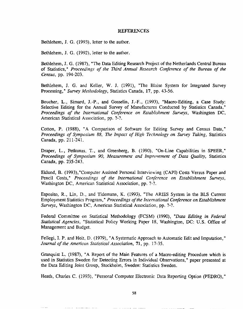
REFERENCES

Bethlehem, J. G. (1993), letter to the author.

Bethlehem, J. G. (1992), letter to the author.

Bethlehem, J. G. (1987), "The Data Editing Research Project of the Netherlands Central Bureauof Statistics," Proceedings of the Third Annual Research Conference of the Bureau of theCensus, pp. 194-203.

Bethlehem, 1. G. and Keller, W. J. (199l), "The Bla.ise System for Integrated SurveyProcessing," Survey Methodology, Statistics Canada, 17, pp. 43-56.

Boucher, L., Simard, J.-P., and Gosselin, J.-F., (1993), "Macro-Editing, a Case Study:Selective Editing for the Annual Survey of Manufactures Conducted by Statistics Canada,"Proceedings of the International Conference on Establishment Surveys, Washington DC,American Statistical Association, pp. ?-?

Cotton, P. (1988), "A Comparison of Software for Editing Survey and Census Data,"Proceedings of Symposium 88, The Impact of High Technology on Survey Taking, StatisticsCanada, pp. 211-241.

Draper, L., Petkunas, T., and Greenberg, B. (1990), "On-Line Capabilities in SPEER,"Proceedings of Symposium 90, Measurement and Improvement of Data Quality, StatisticsCanada, pp. 235-243.

Eklund, B. (1993), "Computer Assisted Personal Interviewing (CAP!) Costs Versus Paper andPencil Costs," Proceedings of the International Conference on Establishment Surveys,Washington DC, American Statistical Association, pp. ?-?

Esposito, R., Lin, D., and Tidemann, K. (1993), "The ARIES System in the BLS CurrentEmployment Statistics Program," Proceedings of the International Conference on EstablishmentSurveys, Washington DC, American Statistical Association, pp. 1-1.

Federal Committee on Statistical Methodology (FCSM) (1990), "Data Editing in FederalStatistical Agencies, "Statistical Policy Working Paper 18, Washington, DC: U.S. Office ofManagement and Budget.

Fellegi, I. P. and Holt, D. (1979), "A Systematic Approach to Automatic Edit and Imputation,"Journal of the American Statistical Association, 71, pp. 17-35.

Granquist L. (1987), "A Report of the Main Features of a Macro-editing Procedure which isused in Statistics Sweden for Detecting Errors in Individual Observations," paper presented atthe Data Editing Joint Group, Stockholm, Sweden: Statistics Sweden.

Heath, Charles C. (1993), "Personal Computer Electronic Data Reporting Option (PEDRO),"

58

Proceedings of the International Conference on Establishment Surveys, Washington DC,American Statistical Association, pp. 1 - 1.

Houston, G. (1993), letter to the author.

Houston, G. and Bruce, A. (1992), "Graphical Editing for Business and Economic Surveys,"unpublished report, Wellington, New Zealand: New Zealand Department of Statistics.

Hundepool, Anco (1993), "Automation in Survey Processing," Proceedings of the InternationalConference on Establishment Surveys, Washington DC, American Statistical Association, pp.1 - 1.

Keller, W. J., Bethlehem, J. G., and Metz, K.-J. (1990), "The Impact of Microcomputers onSurvey Processing at the Netherlands Central Bureau of Statistics," Proceedings of the SixthAnnual Research Conference of the Bureau of the Census, pp. 637-645.

Kovar, J. G. (1993), "Use of Generalized Systems in Editing of Economic Survey Data," toappear in the Bulletin of the International Statistical Institute: Proceedings of the 49th Session,Florence, Italy.

Legault, S. and Roumelis, D. (1992), "The Use of the Generalized Edit and Imputation System(GEIS) for the 1991 Census of Agriculture," Working Paper No. BSMD-92-010E, MethodologyBranch, Ottawa Canada: Statistics Canada.

National Agricultural Statistics Service (NASS) (1992), Report of the Interactive SurveySoftware Committee, "Criteria for the Evaluation of Interactive Survey Software".

Pierzchala, M. (1990a), "A Review of the State of the Art in Automated Data Editing andImputation," Journal of Official Statistics, Statistics Sweden, 6, pp. 355-377.

Pierzchala, M. (1990b), "A Review of Three Editing and Imputation Systems," Proceedings ofthe Survey Research Section, American Statistical Association, pp. 111-120.

Pierzchala, M. (1991), "One Agency's Experience with the Blaise System for Integrated SurveyProcessing," Proceedings of the Survey Research Section, American Statistical Association, pp.767-772.

Stuart, W. J. (1966), "Computer Editing Survey Data - Five Years of Experience in BLSManpower Surveys," Journal of the American Statistical Association, 61, pp. 375-383.

Woefle, L. (1993), "Mixed Mode Data Collection and Data Processing for Economic Surveys,"Proceedings of the International Conference on Establishment Surveys, Washington DC,American Statistical Association, pp. 1 - 1.

59

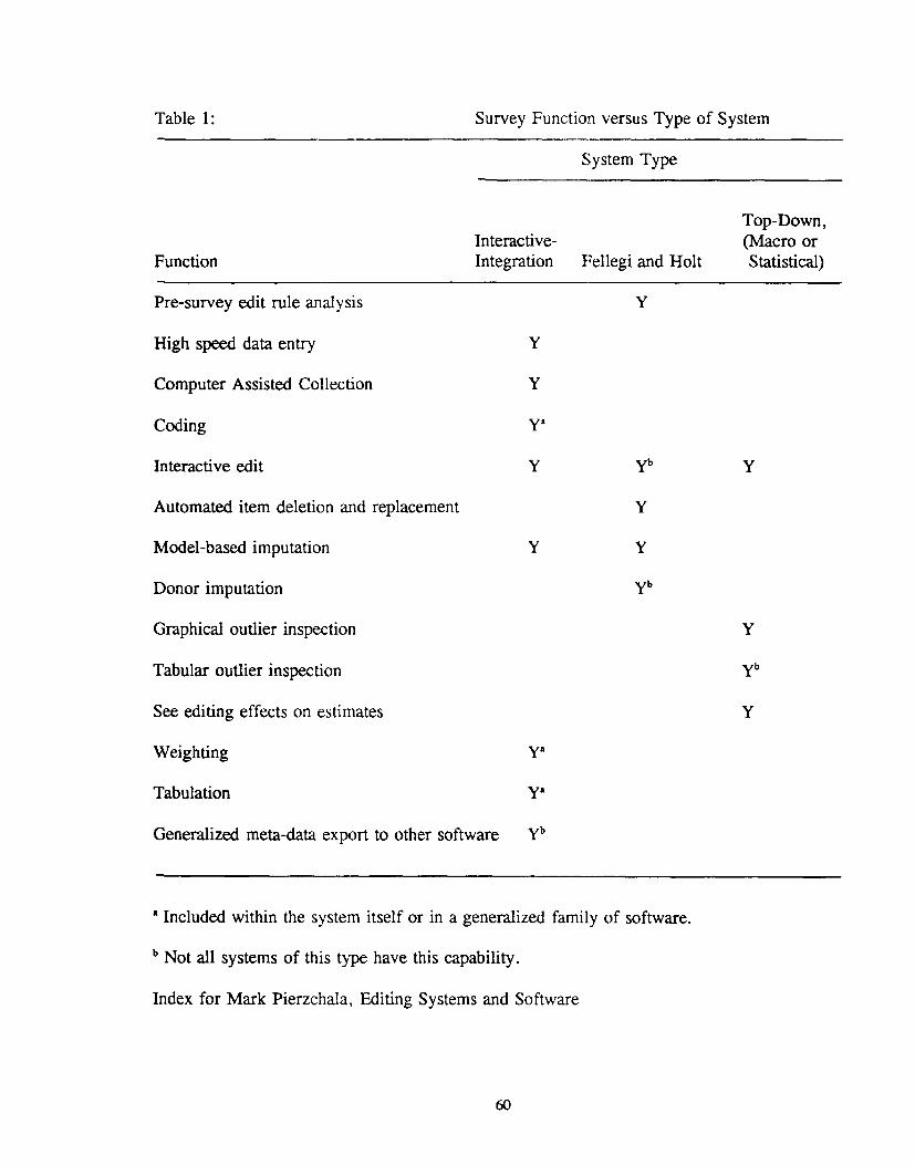
Table I: Survey Function versus Type of System

System Type

Function

Pre-survey edit rule analysis

High speed data entry

Computer Assisted Collection

Coding

Interactive edit

Automated item deletion and replacement

Interactive-Integration Fellegi and Holt

y

y

y

y·y

y

Top-Down,(Macro orStatistical)

y

Model-based imputation y y

Donor imputation yb

Graphical outlier inspection Y

Tabular outlier inspection yb

See editing effects on estimates Y

Weighting y·

Tabulation y·

Generalized meta-data export to other software yb

• Included within the system itself or in a generalized family of software.

b Not all systems of this type have this capability.

Index for Mark Pierzchala, Editing Systems and Software

60

EVALUATION AND CONTROL OF MEASUREMENT ERROR INESTABLISHMENT SURVEYS

Paul BiemerResearch Triangle Institute

Ronald S. FecsoNational Agricultural Statistics Service

1 INTRODUCTION

Survey estimates will almost never be identical to the population value they are tryingto measure as a result of two types of error which are known widely in the survey literatureas sampling error and nonsampling error. Sampling error is the difference between thesurvey estimate and the population value of interest obtained by a census keeping otherconditions similar, that is, error due to surveying only a subset of the population rather thanconducting a complete census of all establishments in the target population. In a completecensus of establishments, the census estimate may still differ considerably from thepopulation value as a result of nonsampling error. Nonsampling error is the difference that isattributable to all other sources not including sampling error--errors arising during theplanning for and the conduct of establishment surveys, as well as during the processing ofthe data and the preparation of the final estimates.

As shown in Figure 1, the sources of nonsampling error may be classified as either(1) specification error, (2) frame errors, (3) nonresponse errors, (4) processing errors, and(5) measurement errors. Specification error occurs when the survey concepts areunmeasurable or ill-defined; the survey objectives are inadequately specified; or the datacollected do not correspond precisely to the specified concepts or target variables. Frameerrors include erroneous inclusions, omissions, and duplications in the sampling frame or inthe sampling process. Also included are errors in listing subunits within establishments insurveys that require subsampling within establishments. Nonresponse errors include unitnonresponse, item nonresponse, or incomplete data. Processing errors refer to the errors inpost-data collection processes such as manual editing, coding, keying, computer editing,weighting, and tabulating the survey data. Finally, measurement error, the topic of thischapter, refers to those errors which occur at the time of data collection.

At a recent conference on the subject, Biemer, et al. (1991) defined surveymeasurement error as:

"... error in survey responses arising from the method of data collection, therespondent, or the questionnaire (or other instrument). It includes the error ina survey response as a result of respondent confusion, ignorance, carelessness,

61

or dishonesty; the error attributable to the interviewer, pershaps as aconsequence of poor or inadequate training, prior expectations regardingrespondents' responses, or deliberate errors; and the error attributable to thewording of the questions in the questionnaire, the order or context in whichthe questions are presented, and the method used to obtain the responses. Atthe time survey responses are collected, all of these factors may intervene andinteract in such a way as to degrade response accuracy."

There are five general sources of measurement error in establishment surveys that willbe discussed in this chapter: (1) the survey instrument, (2) the respondent, (3) theinformation system, (4) the mode of data collection, and (5) the interviewer, if one is used(see Figure I). The survey instrument refers to the survey form or questionnaire and theinstructions to the respondent for supplying the requested information. The respondent refersto the person(s) whose task is to supply the requested information, either by accessing theestablishment's information system or by relying on either their own knowledge or theknowledge of others. Perhaps the most important feature of establishment surveys and onethat distinguishes these surveys from household surveys is a greater reliance on informationor record systems for the required information. These include the establishment's formalrecord systems, company or individual files, and informal records. The mode of datacollection refers to the combination of the communication medium (i.e., telephone, face toface, self-administration, etc.) and the method of data capture (i.e. paper and pencil,computer keyboard, telephone keypad, etc.). Finally, in some establishment surveys, theinterviewer may playa key role in obtaining the information from the establishment andentering the information into the data collection instrument. For some surveys, theinterviewer may simply be a prerecorded voice over the telephone or may be nonexistent forself-administered surveys.

Although all the sources of error in Figure 1 can substantially reduce the accuracy ofsurvey results, our focus in this chapter is on measurement error. Our primary goals are toreview the methods for controling and evaluating measurement error and to study the uses ofthese methods in establishment surveys. Before discussing these methods, two generalmodels for the response process will be briefly reviewed. One model is a cognitive model ofthe response process proposed by Tourangeau (1984) and adapted for establishment surveysby Edwards and Cantor (1991). The second model is a statistical model for measurementerror originally developed by Hansen, Hurwitz, and Bershad (1964). Knowledge of bothmodels is necessary to understand the evaluation and conlIol techniques that will besubsequently described.

62

FIGURE 1 Sources f!f Nonsampling Error

NonsamplingError

I I I I

Specification Frame Nonresponse Processing MeasurementError Error Error Error Error

t i t t-Concepts - Omission -Unit - Editing -Information-Objectives -Inclusion .Within - Data System-Data • Duplication Unit Entry • Setting

Elements .Item • Coding • Mode of• Incomplete • Weights Data

Information • Tabulation Collection- Respondent-Interviewer-Instrument

2 A COGNITIVE MODEL OF ESTABLISHMENT SURVEY RESPONSE

Tourangeau (1984) and, more recently, Eisenhower, et al (1992) described five stagesof the survey response process for household surveys. As depicted in Figure 2, the fivestages are: (1) the encoding of information, (2) comprehension of the survey question, (3)retrieval of information, (4) judgment, and (5) communication. These stages reflect asomewhat idealized paradigm for response which may be described as follows: Informulating a response to a survey question, the respondent must first have the knowledge,belief, or attitude required to provide a valid response (encoding). There must be a sharedmeaning among the researcher, the interviewer, and the respondent with respect to each ofthe words in the question as well as the question as a whole (comprehension). To respond toquestions concerning events or behaviors occurring in the past, the respondent will attempt toretrieve the required information from memory (retrieval of information). Once theinformation has been retrieved, the respondent decides how to respond appropriately, takinginto account risk, benefit, available answer choices, etc. (judgment). Finally, the respondentcommunicates the response to the interviewer (communication). For a single question, therespondent may cycle through some or all of the stages repeatedly as the interviewercontinues to probe for a codable or otherwise satisfactory response.

63

FIGURE 2 Stages of the Response Process

Encoding! Source Decision

Record Formation • records Communication• memory

,

Comprehension ..---. Infonnation --+ JudgmentRetrieval

Adapted from Edwards and Cantor (1991).

As Edwards and Cantor recognized, this response paradigm does not describe atypical response process for an establishment survey. Establishment surveys rely much moreextensively on information (record) systems than do household surveys. As an example,when an establishment survey respondent accesses company records to provide a response fora survey item such as "the number of full time employees during the period (date) to (date)","encoding" and "retrieval of information" take on new meaning. The respondent must haveknowledge of where to obtain the required data. The cognitive encoding of this basicprocedural information is not enough, however, since the required information must havebeen entered in the company's employee record system in order to be retrieved by therespondent. This stage of the response process, which is analogous to cognitive encoding inthe household survey model, is called record Jonnation by Edwards and Cantor. Theretrieval of survey information may require the respondent to invest considerable effort tolocate and access the appropriate record sources. The respondent may have a number ofoptions for responding to the request and the accuracy of the information may varyconsiderably with the effort required to access each potential source. The traditionalhousehold response model does not explicitly account for this source decision stage of theprocess. To account for these differences between the household and establishment surveys'paradigms, Edwards and Cantor proposed a revised response model for establishment surveyswhich explicitly accounts for the establishment survey respondent's reliance on informationsystems rather than recall to respond to survey questions (see Figure 2).

An important benefit of response models is that they allow survey methodologists todecompose the response process into smaller steps that may be treated separately in thedesign and evaluation of surveys. Let us now consider how the response model can be usedas an aid in the control and evaluation of measurement errors in establishment surveys.

2.1 Encoding/Record Fonnation

All establishment survey questions, to some extent, rely on the knowledge, attitudes,and/or beliefs of the respondent. Thus, careless or uncontrolled selection of theestablishment respondent can be an important source of measurement error. The surveyprocedures should clearly specify the minimum qualifications the respondent should posess inorder to be confident in the accuracy of the respondent's reports. An important aspect of theinterviewer's or the addressee's (for mail surveys) task, then, is to identify a respondent

64

meeting these minimum qualifications. In some cases, multiple persons within anestablishment may serve as respondents for various parts of the questionnaire as appropriate.This may necessitate separate questionnaires for each of the respondents, or alternatively, asingle questionnaire may be used with separate sections corresponding to the changes inrespondents. For surveys which rely on information contained in the establishmentinformation system, knowledge of the information system as well as the terms and definitionsof the data items are essential qualifications for the respondent. Ultimately, however, thechoice of respondent is the decision of the establishment's management.

The record formation process is subject to a number of error sources which mayundermine the integrity of the data. Some record systems allow input from multiple sourceswith little or no validation or editing of the input. As an example, university studentenrollment records may be updated by administrative assistants in each college. Errors arecorrected when they are identified as the system is used but no formal system for errordetection may exist. Another common problem in using administrative record systems toobtain survey data is the inconsistency between the record items and the survey items. Therecord system item may include unwanted data components or exclude components which arepart of the survey item definition. The record values may reflect a time frame different thandesired for the survey. The burden on the respondent to adjust for the errors may be sogreat that few are willing to do so.

Incompatibilities between the survey and the establishment record system cansometimes be remedied by revising the survey item definition if respondents are unwilling orunable to revise their record systems. Ponikowski and Meily (1989), in a study of theCurrent Employment Survey (CBS), reported that 59% of the CBS establishments did notadhere entirely to the survey employment definition. The most common problem cited wasthe inclusion of employees on unpaid vacation. Only 56% of the respondents who made thiserror agreed to adjust their figures to correct the error for future waves of the survey.

2.2 Comprehension and Retrieval of Information

The next two stages in the establishment survey response process are comprehensionof the survey question and the retrieval of required information, either from memory or fromrecords. Corby (1984) reports that in a study to evaluate the accuracy of the 1977 EconomicCensuses data, these two stages of the process explained most of the error found in thecensuses data.

Comprehension

Comprehension of the survey question is particularly problematic in establishmentsurveys. Often, the questions contain "legalese" and technical jargon which are not well-understood by all respondents. Further, the questions may require that the respondentaggregate data values across time or other units and it is not clear what components of datashould be included or excluded. The Economic Censuses study provides many examples ofthis. For Annual Payroll in the 1977 Census of Manufactures, the amount of erroneousinclusion and exclusions totaled $3.7 billion or about 2% of the census total. Erroneous

65

exclusion of vacation pay accounted for almost one third of this error. In a study conductedby the National Agricultural Statistics Service (O'Connor, 1993), respondents were asked todefine "calf', a common term in agricultural surveys. Over 30 different meanings wererecorded. Among them were: not yet weaned; up to 800 Ibs; under 600 lbs.; anything undera yearling; under 300 lbs.; everything except stock cows; 8 months or less; and not sure.

Retrieval of Information

Following comprehension, the next stage in the response process is the retrieval ofinformation. Records which contain the required information may be available and accessedby the respondent with some effort. If there are no records or the burden to retrieve theinformation from records is too great, the respondent may attempt to either recall theinformation or to "estimate" the correct response. Eisenhower, et al (1992) and Groves(1989) provide excellent reviews of the literature on recall error. Estimation error accountedfor 75% of the error in the reported value of employment for the 1977 Census of RetailTrade (Corby, 1984). Krosnick and Alwin (1987) suggest that survey respondents"satisfice"; that is, they exert minimal effort in responding to survey questions oftenproviding answers which are "good enough" rather than precise responses. This theory mayoperate both for the retrieval of information from memory as well as the retrieval fromrecords.

2.3 Judgment and Communication

Following comprehension and information retrieval, the last two stages of theresponse process involves the respondent's judgment regarding the appropriate response andcommunication of the response to the interviewer or directly in the instrument. For a closed-ended question, the respondent must decide which response category best fits the informationretrieved in the previous stage. For open-ended responses, the respondent must formulatehis/her own response. The respondent may judge a response as posing some economic orsocial risk or threat and alter the response accordingly.

Response judgment and communication may be influenced by the characteristics of theinterviewer and the interview mode as well as by the instrument. An interviewer who probescompletely and persistently until an acceptable response is obtained can counteract some ofthe effects of satisficing. Deliberate misreporting arising from a perceived economic or legalrisk may be somewhat abated by emphasizing the neutrality of the survey sponsor. For self-administered surveys, the mechanism by which a respondent records his/her response, suchas a laptop computer or telephone keypad, can exacerbate communication problems if it isfaulty or inefficient.

3 A STATISTICAL MODEL FOR ESTABLISH1\IENT SURVEY RESPONSE

The cognitive model of survey response can be used as an aid for understanding andinvestigating the causes of response error in surveys. By considering each stage of theresponse process in the design of a survey, the problems associated with the successfulcompletion of the stage can be identified and mitigated. However, the response model

66

focuses primarily on the respondent. Other factors that may induce measurement error, suchas the interviewer, the mode of data collection, and the instrument, are represented in themodel only through their effects on the respondent. In this section, we consider analternative model which explicitly represents these other error sources. Such a model isuseful for measuring how much of the total error in a survey estimate is attributable to theinterviewer, mode, etc. without regard to which stages of the response process (Figure 2)are affected.

3.1 Sources of Measurement Error

The model postulates that the error in an estimator which is due to measurement erroris attributable to six error sources: (1) the information system, (2) the respondent, (3) themode of data collection, (4) the interviewer, (5) the survey questionnaire or instrument, and(6) the interview setting. As depicted in Figure 3, the respondent is the link between theinterviewer (or instrument, for self-administered surveys) and the establishment informationsystem. Communication through this link may be distorted by the mode of data collection.Each error source may give rise to errors in the reported values. Incorrect data may residein the information system and these data are duplicated in the survey reports. As we haveseen in Section 2, the respondent may give rise to an error at each of the five stages of theresponse process. Errors may be attributable to the mode of data collection in that the datacollected by one mode may be more accurate than that of another. Although the mode doesnot "commit" errors in the way that respondents and interviewers do, the mode may "cause"an error by interfering in or somehow hampering the response process. Likewise, theinstrument or questionnaire may cause errors through the construction and/or position of thequestions, the format/layout of the questionnaire, etc. Finally, the interview setting maycontribute to measurement error through its affects on the response process. The settingincludes such factors as the survey sponsorship, location of the interview, degree ofconfidentiality and privacy perceived by the respondent, and so on. Focusing on these errorsources, as well as on the stages of the response process, allows us to further isolate thecauses of measurement error and to, thereby, understand what actions are necessary toeliminate the causes. A number of statistical methods exist which allow the surveymethodologist to partition the total error into error components corresponding to each sourceand to estimate their magnitudes. In the next two sections, we will present a briefintroduction to these statistical methods.

67

FIGURE 3 Sources of Measurement Error

InformationSystem

Respondent

3.2 A Brief Introduction to Statistical Modeling

Instrument

Interviewer

Several recent references are recommended as introductions to the modeling ofmeasurement error: Groves (1989) Chapter 1, Biemer and Stokes (1991), and Lessler andKalsbeck (1992) Chapter 10. This section provides a brief background in the concepts andnotation of measurement error modeling. These ideas provide the foundation for the errorevaluation and control techniques that will be discussed in Section 4.

Our approach to measurement error modeling is an adaption of earlier work byHansen, Hurwitz, and Madow (1953) and Sukhatme and Seth (1952). The simplest form ofthe model specifies that a single observation, y. , from a randomly selected respondent j , is

J

the sum of two terms: a true value, ~j' and an error, Ej' Mathematically, this may bewritten as

(20.1)

where£j - (0,0;>, ~j - (ll,a~), and all covariances between the terms on the right are zero.Under this model, the variance of the mean, y , of a sample of n observations, ignoring thefmite population correction factor, is

2 2VarG) = ~ + ~

n n(20.2)

where a~ is the finite population variance of the true values and, a; = E(o:) , is the finite

population mean of the individual response variances, of. The term, 0; , is often referred toas the simple response variance (SRV).

Finally, we may define the reliability ratio, R, as

68

R = (20.3)

Since Var(j) = R -1 Var (iL), where iL is the sample mean of the true values. R determinesthe increase in variance of the sample mean or total due to measurement error. R is widelyused as a measure of the stability of the response process. A ratio of R= I indicates total

reliability (a~ = 0) in the measure while a ratio that is near R =0 indicates the lack of

response stability, i. e., the variability among the true values, J1j' in the population is smallrelative to the variability attributable to the response process.

There are a number of extensions of this simple model which serve purposes in theexploration of measurement error. Two extensions which will be considered here are theextension to: (1) accomodate remeasurements of the same sample unit and (2) incorporatemultiple sources of measurement error.

Extension for Reinterview Data

Some methods for evaluating measurement error require at least two measurements onsome of the sample units. Let Yja.denote the observation on unit j on the a;-th occasion.Extending (1) we have

(20.4)

where eja. - (O,at«) and we assume that the covariance involving the terms on the right arezero both between trials and within trials.

A special case of (4) assumes that at« = at, a; = 1,2, that is, the second trialproduces responses which are distributed identically to the responses of the first trial. Thismodel is usually assumed for reinterview studies where the second interview is intended to bean independent replication of the first interview. Under these assumptions, an estimator ofthe SRV is

0; = L (Yjl - Yj2)2/2nj

69

(20.5)

and an estimator of R is (1- a~a~) where a~ is the average of

a~1I ::::Lj (Yjll -YIl)2/ (n-1), for a: ::::1,2.There are a number of reasons why the assumptions for (4) may not be satisfied in practice(discussed further in Section 4.4).

Another use of the model in (4) is the estimation of measurement error bias usingrecord check studies or true value reinterviews. For this purpose, the assumptions associated

with the error term, Ej« ' are altered. Instead, assume Ej1 - (Bpot) and Ej2=O. That is,assume that the error associated with the first observation has a non-zero mean (referred toas measurement bias) denoted by Bj and that the second observation has no error. Under thismodel

E(Y) ::::B (20.6)

where B ::::E(B.) , the measurement bias in the estimator y. Thus, the aim of studies whichJ

employ (4) under this set of assumptions is to estimate B. Under the model assumptions, thebias can be estimated by

(20.7)

Again, there may be severe difficulties in designing evaluation studies which satisfy the "truevalue" assumptions (discussed subsequently in Section 4.3).

Extensions to Incorporate Error Sources

The statistical models discussed previously do not explicitly provide for thepartitioning of the error variance or bias into separate components corresponding to the fiveerror sources in Figure 3. For example, suppose we wish to investigate the contribution tothe error variance due to interviewers. To accomplish this, letYij denote the responseobtained from the j-th respondent in the i-th interviewer's assignment. Then partition theerror as Eij ::::hi + eij where hi is a random error variable associated with interviewer iand eij is the difference eij = E ij - hi' Substituting this erTor term into (1) we have

(20.8)

where hi - (O,o~ ,eij - (0,0;) , and as before, all terms on the right are uncorrelated. If wefurther assume that interviewer assignments are interpenetrated, that is, each assignment is a

70

random subsample of the initial sample, then the model can be rewritten as the traditionalANOV A model; viz.,

(20.9)

wheree: = eij + (~ij-~) , e: -(O,a~/) and ~ is a fixed constant. Using ANOV A methods,

the interviewer variance, a;, can be estimated as a function of the between and withininterviewers sums of squares (see Groves, 1989, p. 318).

A useful measure of the contribution of interviewers to the error variance is

Py = (20.10)

referred to as the intra-interviewer correlation. An estimator of Py is also available fromthe analysis of variance of interviewers.

The model (9) can be readily extended to include other sources of error that may beviewed as random effects. Examples are coders, editors, and supervisors. Additional usesof this model are discussed in Section 4.2.

When the model effects associated with an error source must be considered not asrandom variables but as fixed effects, a slightly different model is more appropriate. Forexample, we may be interested in three particular modes of data collection or two alternativequestion wordings. Further, we may be interested in the response reliability under thealternative modes or question versions as well as their contributions to response bias. To fixthe ideas, we shall consider a model appropriate for investigating mode effects.

Rewrite model (8) as

y .. = ~ .. + M. + e..IJ I.J I IJ

(20.11)

where now Yij is the response of the j-th respondent assigned to the i-th mode and Mj is aconstant effect associated with the i-th mode. Again, by randomly assigning respondents tomodes, we may invoke the ANOV A model for analyzing the mode "biases." Under this

model, the mode "differential biases," M. - M",i ""i' are estimable but the biases are notI I

unless one assumes thatMj = 0 for some i. As an example, in a study of the effects of faceto face interviewing, telephone interviewing, and mail self-administered methods, we may be

71

willing to assume that the bias associated with face to face interviewing is zero for somecharacteristics. In this case, the mode biases associated with the other two modes areestimable.

Finally, we may be interested in comparing the reliability ratios, Ri ' associated withalternative modes or questionnaire versions. For this objective, we extend the model (3.11)for repeated measurements in analogy to (4) as follows:

y .. == Il .. + M. + e ..vo: r V I IJ4(20.12)

and assume eijo: - (O'0'~4)' The reinterview methods described earlier may be used to obtain

estimates of a: and, thus, Ri •

4 SOl\ffi TECHNIQUES FOR ERROR EVALVATION AND CONTROL

In this section, we briefly describe a number of techniques for evaluating andcontrolling components of the measurement error models described previously and provideexamples of their use. The methods discussed are: (1) cognitive laboratory methods, (2)experimental design, (3) observational studies, (4) administrative record check studies, (5)true value reinterview studies,(6) replicated reinterview studies, and (7) external and internalconsistency studies.

72

4.1 Cognitive Laboratory Methods

Cognitive methods encompass a wide array of exploratory techniques for either (1)investigating one or more components of the cognitive response model in Figure 2 or (2)identifying the types of errors that may be introduced during data collection. In cognitivelaboratory methods, the objective is usually to obtain information on the causes of error andthe ways in which alternative survey methods or design features affect survey response.Laboratory studies usually involve small sample sizes (less than 100 subjects) and, becausethese studies are usually conducted at a small number of sites where survey conditions can betightly controlled, nonrandom or restricted random samples. Therefore, it is usually notpossible to draw inferences regarding the magnitudes of measurement error components fromthese studies. For inferring the magnitudes of error, field studies, observational studies, orembedded survey experiments, to be discussed subsequently, are much more effective.

Forsyth and Lessler (1991) provide a comprehensive summary of the cognitivelaboratory methods which have been used in demographic surveys. However, documentedapplications of cognitive laboratory methods to establishment survey methodology are relativerare. In Chapter XX, Dippo, Chun, and Sander describe the recent research in theapplication of some of these methods to establishment surveys.

4.2 Experimental Design and Observational Studies

Whether it be an investigation of alternative modes of interview, a test of alternativequestion wordings, or the estimation of interview effects, randomized experimental designhas played a pivotal role in the development of measurement error theory and methods. Inone of the earliest uses of experimental design, Mahalonobis (1946) randomized(interpenetrated) interviewer assignments in an agricultural survey in order to obtainevidence of interviewer biases. Hansen, Hurwitz and Bershad (1961); Fellegi (1964); andBailar and Dalenius (1969) formalized and further developed the method of interpenetration.The discussion in Section 3.2 regarding the use of ANOVA for estimating interviewervariance is a special case of this more general methodology.

The use of randomized experimental designs in full scale surveys is referred to as anembedded experiment. Experimental designs have also been used in small scale field testsand in cognitive laboratory experiments. In the laboratory, where the experimentalmanipulation of survey conditions is easier, designs with very complex treatment structuresare possible. For example, O'Reilly, et al. (1993) describes a laboratory study employingan incomplete block, repeated measures design in which three alternative modes of datacollection were tested.

In the field, treatments are typically simpler, simultaneously manipulating only one ortwo experimental conditions. However, the randomization of experimental units may beconsiderably more complex. As an example, in a test of two types of interviewer trainingand two modes of data collection, interviewer training types may be randomly assigned toprimary sampling units while the mode of interview treatment may be randomly assigned toestablishments within the interviewer assignments.

73

In many situations, the required randomizations and experimental manipulations wouldbe too expensive, too impractical, or simply impossible to perform and "nonexperimental" orobservational studies are conducted. As an example, to answer questions about a possiblecausal relationship between the position of the survey respondent within the establishmentand the accuracy of responses to a mail questionnaire, an experimental study would need tocontrol who in the establishment completes the questionnaire for a large number ofestablishments over a considerable time period. Due to the difficulties of controlling such anexperimental assignment of respondents as well as the costs, an experimental study is notfeasible. Further, the results of such a study may be affected by the effort exerted by theresearchers to control the type of respondent. Although the researcher may instruct theestablishment as to whom should complete the instrument, this is ultimately decided withinthe establishment.

In an observational study, the survey proceeds normally without experimentallymanipulating the type of respondent. Rather, when the returns are received, the reseacherobserves the position of the respondent in the establishment and relates this variable toresponse accuracy in much the same way as in an experimental analysis. For example, wemay have observed that response accuracy tended to be better for members of theestablishment's clerical staff than for members of the management team. However, we maythen ask whether this result has as much to do with the establishment's size as it does withthe respondent's position. In larger establishments, special clerical positions may beestablished for the purpose of furnishing accounting information for regulatory purposes,while in smaller establishments where such managerial luxuries are not affordable, the taskfalls to the busy proprietor or his/her spouse. To examine this possibility and other similarones, explanatory variables, such as establishment size, are incorportated in the analysis toeliminate these as causes of the observed relationship. Of course, there is always the riskthat some important explanatory variable escapes the researcher's attention or is not availableto be incorporated into the analysis and conclusions regarding causality will be misleading.The literature on causal modeling (see Stolzenberg and Land, 1983, for a review) provides aset of methods and principles for making causal inferences using observational data.

4.3 Admini~rative Record Check and True Value Reinterview Studies

While cognitive methods may provide valuable insights into the response process, it isoften desirable to estimate the magnitude of measurement bias. To do this requires that thetrue value of the characteristic be known. With such information, faulty data items can beidentified, measurement variance and bias can be estimated, and, in some cases, the sourcesand causes of error can be determined. As described earlier in Section 3.2, record check andtrue value reinterview studies are the two most widely use.d techniques for estimatingmeasurement bias.

Administrative Record Check Studies

Because of the unavailability or inaccessibility of relevant administrative data for thecharacteristics typically measured in establishment surveys, and the expense of obtainingrecords from official sources, record check studies occur relatively infrequently. For this

74

technique, survey responses are compared to administrative records such as federal/stateincome or sales tax reports, licensing information, or other government data. Privacylimitations and differences in record-keeping and reporting requirements often limit theability to make suitable administrative matching studies. In one type of record check study,a sample of establishments is drawn from the establishment frame and then the correspondingadministrative records are located. Alternatively, we may start with a sample of records andthen interview the corresponding establishments. The later is usually more efficient becausethe precision for rare items can be better controlled. While selecting records from the filesof accountants and other financial services can be inexpensive, the coverage of the populationcan be poor. For example, Willimack (1989) found that only about 11 percent of farmersreported using financial services.

An implicit assumption of the administrative record check method is that the recordscontain accurate information (i.e. true values) for the survey charateristics of interest.Under this assumption, estimates of B can be obtained as in (7). However, three problemstypically plague the method and limit the usefulness of the records data:

• The time periods for the record data and the survey data may not coincide,

• The characteristic(s) being reported in the record system may not exactly agreewith the characteristic(s) being measured in the surveys, and

• To save evaluation study costs, the records study may be confined to a veryrestricted geographic area and inferences beyond this restricted population maybe invalid.

The study by the Federal Committee on Statistical Methodology (1983) provides someguidance on methodological requirements to conduct record checks. Further, Ponikowskiand Meily (1989) provide an application where data on employment, earnings, and hoursworked reported by establishments in the Current Employment Statistics survey wereexamined.

"True Value" Reinterview

When accessing administrative records is not feasible because of their availability,cost, privacy concerns or other reasons, a reinterview approach which aims to obtain the truevalues of survey variable is an alternative. In the reinterview, more time may be taken andgreater attention given to the reporting task in an effort to obtain highly accurate data and toreconcile originally reported data against a reinterview report. Reinterview may require thatrespondents' access company records for "book values" whenever they are available. Yet,many small businesses may keep records informally in a "shoebox" file. Willimack (1989)found that 25 percent of U.S. farm operators used such informal records, while only 3percent used a computer, and 16 percent used a formal workbook.

In household surveys, it is well-known that obtaining a true value during reinterviewis very difficult, and, indeed for some variables such as attitudinal data, true values may not

75

exist. Establishment data, while seeming to be more factually based, still presents challengesfor reinterviews. For example, Van Nest (1985) found that when computer records did notkeep breakdowns of data such as expenditures for new versus used equipment, true valuesfor the detailed data could not be obtained.

The reinterview designs vary depending on assumptions which are most reasonablefor the particular data and survey. Because the reinterview is often combined withinterviewer performance evaluation, the reinterviewer is often the supervisor of the originalinterviewer. Forsman and Schreiner (1991) discuss some of the difficulties associated withthis practice. Alternatively, "more experienced" interviewers have been used provided thatthey do not reinterview respondents whom they previously interviewed. Althoughreinterviews conducted by telephone are less costly, some data might best be obtained in apersonal interview to ensure records are consulted. Cantwell, et al. (1992) list questionswhich need to be resolved when designing a true value reinterview, including:

• How should the reinterview be introduced to the respondent?• Should there be prior notification of reinterview?• How soon after the original response should the reinterview take

place?• Should question wording be identical?• How much burden should be placed on respondents?• Should proxy responses be allowed in reinterview?• Should the respondent or the reinterviewer determine whether the

original response or the reinterview response (or neither) iscorrect?

The Census Bureau used true value reinterviews to study the accuracy of data ineconomic censuses (Corby, 1984; 1985). For this study, one of the characteristics of interestwas operating expenses including components such as cost for purchased advertising,unemployment compensation paid, and so on. The measurement biases were estimated foreach component and then these were combined and later used to correct the reported data.An interesting aspect of the study was the classification of the reinterview responses intothree categories: (1) book figures or values the respondent obtained directly from companyrecords; (2) estimated values deemed reliable by the reinterviewer, and (3) estimated valuesdeemed unreliable by the reinterviewer. For unreliable items, the respondent was asked toprovide a range of values to include the highest and lowest value the true figure could take.

Another example is provided by Fecso and Pafford (1988) from a reinterview studyused to measure bias in a National Agricultural Statistics Service (NASS) survey. Because ofthe detailed nature of acreage, stocks and livestock inventory items, NASS has reliedprimarily on personal interviews in the past to get the most accurate answers from the farmpopulation. For example, in collecting on-farm grain stocks data, farmers may store grainsin multiple bins on property they own and/or rent. In addition, farmers often are involved inmultiple operating arrangements involving their own grains, those of landlords, and thosewhere formal and informal partnerships exist. Like many survey organizations faced withcost containment and the desire to publish survey results more quickly, NASS has switched

76

to more extensive use of telephoning, including CATI to collect these data. Obtainingaccurate responses by phone was considered a problem not only because of the detailednature of these data, but also because the centralized state telephoning crews lack thefamiliarity with farm terms that a personal interviewer, recruited from the local farmcommunity, might have.

The focus in the study was to estimate the measurement bias by treating the finalreconciled response between the CATI and independent personal reinterview response as the"truth." In order to obtain "truth" measures, experienced supervisory field enumerators wereused in reinterviewing approximately 1,000 farm operations for the 1986 DecemberAgricultural Survey. This study of corn and soybean stocks in three states indicates that thedifference in the CATI and final reconciled responses, the bias, was significant for all butone item (soybean stocks in Indiana). The direction of the bias indicates that the CATI datacollection mode tends to underestimate stocks of corn and soybeans.

In the process of reconciliation, the reasons for differences were collected. Table 1indicates that an overwhelming percent of differences, 41.1 %, could be related to definitionalproblems (bias related discrepancies), and not those of simple response variance (randomfluctuation). Examples of these definitional problems are rented bins or grain belonging tosomeone else not included, confusion with reporting government reserve grains, and bins onson's farm mistakenly included. Definitional discrepancies were the largest contributors tothe large bias. In contrast, the differences due to rounding and estimating contributed littleto the overall bias.

Table 1 Reason for Differences in CATI and Reinterview Responses forCorn Stocks in Minnesota - December 1987

Reason

Estimated/Rounding

"Definitional"

Other

Total

Source: Fecso and Pafford (1988).

Number

2837

2590

Percentof

Total

31.1%

41.1%

27.8%

100.0%

The report suggests that the bias in the survey estimate generated from the CATItelephone sample might be reduced through a revised questionnaire design, improvedtraining, or a shift in mode of data collection back to more personal interviews. Consideringthe constraints of time and budget, the change to additional personal interviews is unlikely.Thus, the alternative suggested was to use reinterview techniques to monitor this bias overtime and to determine whether the bias has been reduced through improvement in

77

questionnaires and/or training. If large discrepancies continued the estimates for grain stockscould be adjusted for bias through a continuing reinterview program.

4.4 Replicated Reinterview Studies for Measuring Reliability

In (3), the reliability ratio, R, was defined as the ratio of the variance of thepopulation of true values to the total variance, including measurement variance. Estimationof R typically involves obtaining replicated measurements on a subsample of units via a

reinterview study. In order for the estimator in (5) to be unbiased for 0; , two assumptionsmust hold for the reinterview survey: (1) the mean and variance of the response error

associated with the reinterview and the original interview are identical; i.e., E«i - (j.1e'o:)

for a = 1,2, and (2) the covariance between the errors E Ii and Eli is zero.

Assumption (1) requires that the reinterview survey create the same general surveyconditions that existed in the original interview, i.e., the same survey questions, type ofinterviewers, mode of interview, respondent rules, and so on. However, since reinterviewsurveys must necessarily be conducted at a later point in time, the survey questions may needmodification to account for the time difference. Further, to save cost and respondent burden,only a subset of the original questionnaire may be used. If the original survey wasconducted in-person, the reinterview may not be affordable unless it is conducted by a lessexpensive mode. Other changes in the reinterview procedures may be required to save costs.The consequences of these changes may affect the response error distribution thusinvalidating assumption (1). In household surveys, this assumption has been well-tested andit appears that this condition is achievable in most situations (see, for example, Forsman andSchreiner, 1992, and Groves, 1989). For establishment surveys, reportd research onreinterview assumptions is scant, yet assumption (1) seems plausible for a well-designedestablishment reinterview survey.

Assumption (2), however, is much more problematic. Errors between trials may becorrelated due to a number of factors. Respondents may recall their original responses andsimply repeat them in the reinterview without regard to their accuracy. If the error isrecorded in the company's record system, the error will be replicated if the same recordsystem is accessed in reinterview, or they may repeat the same response process to arrive atan answer. Thus, it is likely that the errors in the two responses are of similar magnitudeand direction, inducing a positive correlation between the errors. For household surveys,O'Muircheartaigh (1992) reports correlations as high as 57 per cent in the CPSunemployment classification. However, little is known regarding the between trialcorrelation for surveys of establishments. Bushery, et.al. (1992) discusses the difficulties ofimplementing a reinterview by mail when the original survey was conducted by mail. In asurvey of schools, they found evidence that respondents who kept a copy of their originalresponses transcribed these responses to the reinterview form.

It can be shown that, for a between trial correlation of T, the relative bias in theestimate of the SRV in (5), is -T. Thus, a positive correla.tion results in a downward bias in

78

the estimates of reliability. More research is needed to study the magnitude and direction ofT for characteristics measured in establishment reinterview surveys.

4.5 Internal and External Consistency Studies

Two general techniques for assessing measurement error (at times in combination withother sources of NSE) are internal and external consistency checks. Internal consistencystudies include analysis of edit output and analysis allowed by the use of rotating paneldesigns. External consistency studies consists of a comparison of the estimate withcomparable estimates from another source, done most effectively when compared as a datasenes.

External Consistency Studies

The comparison of several series of estimates can provide an indication thatmeasurement error may exist. If sampling error is small enough, then deviations in theprofile of the series would indicate a problem with NSE. Similarly, a difference in the levelbetween the series is an indication of NSE. If one series is considered very accurate andanother series is parellel but at a different level, the difference is a crude estimate of overallbias. In crop yield surveys conducted in the U.S., time series produced by differentmeasurement methods (counts from fields or various farmer reporting techniques) are oftenvery parallel, but some level differences of 10 percent occur (Fecso, 1991). Unfortunately,determining the contribution to observed NSE due to measurement error is not possiblewithout other sources of information. In an example of an external series comparison,Silverberg (1983) examined several of the many different series of estimates of retail gasolineprices. He found that all the national estimates of retail motor gasoline prices were within 5percent of the EIA series, but sizable differences existed for wholesale prices in some series(although he speculates that the differences may be due to a difference in volume weightedprice estimates versus a price based on a price index). Further, Silverberg found thatinternal assessments were more informative than external comparisons.

Internal Consistency Studies

Internal consistency studies are often exploratory in nature. Activities during editingmay lead to the most familiar forms of internal consistency study. A detailed description ofediting processes can be found in the chapter by Granquist (19940. In a study of U.S.federal establishment surveys (Federal Committee on Statistical Methodology, 1988), almostall of the surveys reviewed used practices such as analyst review of the data and edits forreasonableness with followup proceedures in efforts to control response error. About three-quarters of these surveys compute edit failure rates and about half compute interviewer errorrates as an inderect technique to measure response error. The information about the relativemagnitude of potential measurement error gleaned from analysis of these error rates andfrom feedback from respondents and interviewers can help target areas in need of moredirect measurement using methods previously described.

79

For most surveys, these edit failure rates relate to procedures tending to be based onlogical relationships among data items and experience with range checks to detect outliers.More statistically based procedures to identify unusual data are available. Such techniquescan be useful in associating potential causes of measurement error with the errors. Barnett(1983), for example, discusses principles and statistically based methods, includingmultivariate approaches, for detecting outliers in data sets. Silverberg presents a graphicaltechnique for examining the changes over time in the distribution of company reported pricesof gasoline. Temporal comparison of response distributions is useful in detecting unexpectedchanges to conditions impacting response or, as Silverberg found, verifying expected changessuch as greater price variability during the 1979 oil crisis.

Repeated use of the same establishment and data item in surveys conductedperiodically provides an opportunity to measure validity and reliability of the data. Saris andAndrews (1991) and Munck (1991) discuss the use of structural modeling as an approach toevaluation of measurement errors. Reiser et. al. (1992) apply such models in a study ofmeasurement error in a com yield study in the U.S. Variables which were easy for theenumerator to count, such as number of stalks, were found to be highly reliable, but somemeasurements, such as length of the ear, were not.

In research on the use of historic data, methodology very similar to a reinterviewapproach, Pafford (1986) studied the effect of using farmer-reported planted acreage from aspring survey during the fall survey interview. Differences in planted acreage between thespring and fall survey were largest in the control treatment where prior responses were notused. When spring reported data was worded directly into the fall question, the differenceswere smallest. The control group had more instances of unreported acreage in either of thesurvey periods, while there were few reports of zero acreage when the spring report wasnonzero and incorporated into the fall question. While interviewers had no problems usingprior data and response variance between surveys decreased, a recommendation to usehistoric data could not be made because there was no way to determine which treatment hadlower response bias. Similar results were found in a later study of grain stocks(pafford, 1988).

4.6 Quality Standards

The establishment and use of standards are viewed by many as fundamental needs fora process of quality improvement. Standards reflect principles that are commonly held forguiding and assessing the quality of an activity. In a survey environment, standards are theguide to the process that keeps an organization focused on the essential conditions andprocedures that could produce unwanted changes in measurements. Morganstein and Hansen(1990) indicate that without clearly stated standards, followed without compromise, increasedand unnecessary variability will be a result. Areas where standards are believed to be usefulin controlling measurement error include the design of the survey instrument, recruitment ofand training of enumerators, supervision of interviews, and editing.

Freedman (1990) notes that standards alone cannot improve data quality.Enforcement, education, and evaluation are also necessary, as is the commitment from

80

everyone in the organization. Further, the organization must decide where standards areneeded. In doing this, EIA used accuracy, consistency, efficiency, and clarity as guidingprinciples. Some standards apply regardless of the subject matter covered in the survey, forexample pretesting all questionnaires to assure clear wording of questions and therespondents ability to understand and answer the question. Others depend upon thecircumstances of the survey, such as the need for interviewers not to know the name of theorganization sponsoring the survey when the data will be used as evidence in judicial actions(Morgan, 1990). Examples of organizations with very detailed standards for instrumentdesign and collection activities include the Energy Information Administration (1989) and theNational Center for Education Statistics (Cooperative Education and Data Collection andReporting Standards Project Task Force, 1991). Many agencies do not have formallydeveloped standards for data quality. Further, these studies suggest that the development ofstandards may often be the response by organizations in which data quality problems haveescalated to a crisis.

EIA uses a quality audit to check for compliance with standards. The audits focus ondetermination of the soundness of the data system and its ability to produce data that meetsstandards (acceptable quality). Reviews and tests of survey processes are made anddocumentation is reviewed. Checklists are used to ensure coverage of all standards and tonote deviations. Offices are held responsible for implementing the recommendations madeby the standards review team when deficiencies are found. However, while enforcementmay be necessary to ensure that the standards are followed as intended, there is someconcern that auditors may be looked upon as the "quality police" of the organization and aresentment could build. For quality standards to work, a cooperative environment built upontrust, voluntary self-improvement, and an emphasis on organizational goals and missions isnecessary. Such efforts are the emphasis of the growing movement from inspection samplingof the final product toward quality improvement strategies.

5 SUMMARY AND CONCLUSIONS

In this paper, we have attempted to provide an overview of the most importantmethods for evaluating measurement errors and a description of how they have been or couldbe applied to establishment surveys. We presented a number of models for measurementerror which are useful for guiding efforts to improve survey data quality. We presentederror evaluation methods, such as cognitve laboratory techniques, which may be appliedduring the design stages of a survey. Other methods presented, such as reinterviews,experimental designs, and observational studies, may be applied during the execution of thesurvey. However, the results of the latter evaluations are not known until after the survey iscompleted. Finally, post-survey methods such as internal and external validity studies andadministrative record check studies were discussed in the context of establishment surveys.One area not addressed directly in this paper is evaluation methods that may be appliedduring data collection in order to provide timely information on the quality of the data as it iscollected. The need for such methods is obvious. In order to be controlled, survey errorsmust first be measured and measured continuously during the course of the survey. Wheninformation on data quality is available on a "real time' basis, survey managers can

81

determine the degree to which errors are being controlled and can intervene if action isneeded reduce the errors. Such methods are called process quality control methods.

It is quite unusual that a component of measurement error can be directly estimatedand monitored continuously during data collection. What is usually the case is that someindicator of data quality - response rate, edit failure rate, item nonresponse rate, etc. - ismeasured and monitored. A quality indicator may be any quantity that can be routinelyobserved that is correlated with some component of error. As an example, interviewer editfailure rates may be correlated with interviewer variance or bias. The belief is that keepingthe indicators within acceptable limits will also control the corresponding mean squared errorcomponent, resulting in data which are of higher quality and value. Unfortunately, there isno assurance of this and studies which directly measure bias and variance components arestill needed to determine the true level of data quality. Further, many serious measurementerrors can only be detected using direct approaches. In continuing surveys, evaluating themagnitudes of the measurement errors periodically (say once every two or three years) maybe adequate to ensure that the routine quality control practices are controlling errors at thedesired levels. For one time surveys, direct evaluation studies may be expensive but stillnecessary for two purposes: (1) to provide data users with an accurate assessment of thedata's true information content and (2) to obtain information on survey error that can be usedin future surveys. There is a vast literature on methods for quality improvement in industrialor service settings, but only a few articles specifically for survey operations (e.g. Fecso,1989; Colledge and March, 1992).

While a variety of methods are available for the control of data quality, the use of themethodology varies. The Federal Committee on Statistical Methodology (1988) profiles theuse of various measurements and control procedures for measurement error in federalestablishment surveys. A majority of the surveys studied reported the use of editing, analystreview, and the production of edit failure rates. Useful techniques such as reinterviews,record check studies, and cognitive studies were reported as rarely used. In general there isa tendency to look at indirect measures rather than direct measures of error components.The lack of standard approaches to incorporating error measurement strategies into surveysmay, in part, have stimulated the recent interest in total quality management (TQM)approaches in some survey organizations. Federal agencies are further motivated to useTQM approaches because recent administrations have encouraged such thinking govemment-wide.

A TQM strategy of management emphasizes a focus on continuous improvement in allaspects of an organization. The framework for such a strategy includes the followingelements (Fecso, 1993):

• identify customers and their needs,• move from only measuring quality to improving it,• base decisions on the analyses of data,• anticipate and accept change,• emphasize an inter-organizational team approach to problem solving,

82

• ensure that staff are all aware and involved in the organization's quality goals,and

• accomplish the above activities with top management leadership.

While the survey research literature has many reports on the use of techniquesassociated with TQM in various situations or in units of a survey organization, the literatureis devoid of studies about the effectiveness of the efforts as an strategy in surveyorganizations. One might expect this since most survey organizations appear to be in thedevelopment stages of implementation during which they focus on training and teamformation. In subsequent stages, we would expect open discussions leading to agreement onthe most important quality problems in the organization, further use of real-timemeasurements during the survey process, increasing communication of the results with thoseinvolved in the operations, and delegation of responsibility for taking actions to correctproblems.

Quality prof1les can be very helpful in quality improvement efforts, yet profiles whichconsist only of indirect measures of data quality can be quite misleading (Bailar, 1983). Useof the models and techniques described in this paper are also necessary for error evaluationsand data quality improvement. The Federal Committee's report convincingly demonstratesthe need for more frequent use of the evaluation methods describe in this paper withFederally sponsored establishment surveys. In the private sector were studies which directlyevaluate the components of measurement error are seldom reported, the need is even greater.

83

ENSURING QUALITY IN U.S. AGRICULTURAL LIST FRAMES!

Cynthia Z.F. Clark, National Agricultural Statistics Service, Elizabeth Ann Vacca, Census BureauCynthia Z.F. Clark, NASS, 14th & Independence Ave., Washington, D.C.

KEY WORDS: Business registers, record linkage,census and survey list frames

ABSTRACT

In the United States, agricultural data arecollected by the Bureau of the Census in theDepartment of Commerce, and the NationalAgricultural Statistics Service in the Deparnnent ofAgriculture. Both agencies are mandated by law tocollect data on the agricultural economy. Title 13 ofthe United States Code (USC) requires the CensusBureau to conduct a quinquennial census of agriculture,providing detailed data on agricultural operatioIl<; foreach county. USC Title 7 requires the NationalAgricultural Statistics Service to collect data onagriculture and its market. The census of agriculturehas mandatory data reporting requirements whereassurveys conducted by the NASS have voluntaryparticipation.

Both agencies are required to protect theconfidentiality of the individual record data but aresubject to different legal requirements. Title 13restricts access to census data to sworn officials andcensus employees, prohibiting the release of the censusof agriculture list or census data to the NASS, or to anyother organization. Title 7 permits the use of datacollected by NASS for statistical purposes, and thusenables the Census Bureau to use the NASS list inbuilding the census list. The NASS list, however, doesnot have complete coverage of the universe of farmoperations. Thus, it is necessary for each agency tocompile its own list frame to meet its mandatedstatistical needs.

Both U.S. agencies use the same definition ofa farm - a place from which $1,000 or more ofagricultural products were sold during a calendar year.A new census list is created every five years by linkingagricultural statistical, administrative, and commoditylists of establishments. The NASS list was developedin the late 1970's from similar types of lists and iscontinually maintained. TIle overall quality of bothcensus and survey data is dependent upon the quality ofthe list frames. The paper focuses on five attributes of

list frames - scope, accuracy, duplication, coverage,and cost efficiency - relating to quality. Listdevelopment procedures and quality indicators arediscussed and compared.

1. AGRICULTURE CENSUS LIST FRAME

Since 1969 the census of agriculture has beenconducted using a mail-outJmail-back data collectionprocedure in lieu of personal enumeration. Prior toeach census, the Census Bureau assembles records ofindividuals, businesses, and organizations identified ashaving some association with agriculture. This includesfiles from the previous census, administrative records ofthe Internal Revenue Service (IRS) and the SocialSecurity Administration (SSA), and statistical records ofNASS. Additionally, lists are obtained for specializedoperations (e.g. nurseries and greenhouses, specialtycrop farms, poultry farms, fish farms, livestock farms,cattle feedlot operations, grazing permittees) from Stateand Federal government agencies, trade associations,and similar organizations. Lists of companies havingmultiple establishments (or locations) producingagricultural products are obtained from previouscensuses and updated using the information from theStandard Statistical Establishment List maintained by theCensus Bureau.

After the various address lists are acquired, theCensus Bureau performs record linkage to removeduplicate addresses, screens for nonfarm records, andprepares mail labels for each address. Five majoroperations are required for record linkage: format andstandardization, business or personal identificationnumber linkage (Employer Identification Number, ErN,or Social Security Number, SSN), geographic codingand ZIP code verification, alphabetic name linkage, andclerical review of potential duplicate record sets. Forthe past four censuses, two similar phases of addresslinkage were conducted to permit incorporating morecurrent addresses than would have been available usinga single linkage.

The format and standardization operationplaces each source record into a common format; editsthe source records; and assigns name control,

'This paper reports the general results ofresearch undertaken by the staff of the Census Bureau and the National AgriculturalStatistics Service. The views expressed are attributable to the authors and do not necessarily reflect those of the Census Bureauor the NASS.

84

processing codes and size codes to each record(Gaulden, 1990). The name control uses the first fourcharacters of the primary name, containing a minimalof three non-numeric characters, not appearing in aspecial agricultural "skip list" dictionary. Thisdictionary contains over 1,000 words and abbreviations(such as Farm, Dairy, Bros) which could conceivablyappear in the name field but were not likely to be thesurname.

Processing codes facilitate the use of the mostreliable information in the final list record. Initially,each record is assigned a name and address prioritycode based on the expected currency of the addressinformation of the record source. During recordlinkage, the name and address of the record within alinked record set with the highest priority is retained.Each record is also assigned a size code based on theestimated total value of agricultural products (TVP) tobe sold in the census year derived from agricultural dataon the source record. During record linkage, the sizecode from each record in linked record sets istransferred from each of the deleted duplicate records tothe retained record. This allowed for the derivation ofboth a "source combination code" indicating all thesources for the final record and a "final size code"based on the reliability of size information for eachsource.

Records are then linked by computer on EINand SSN. All remaining unmatched and potentialduplicate records have the addresses coded bygeographic area, the names identified according to part,and the names coded using SOUNDEX procedures(where vowels and double consonants are deleted fromnames). The geographic coding system was designedto ensure that all records contained standardized andedited geographic codes, prior to record linkage. Thename and address linkage procedure adapted theFellegi-Sunter probability model relying on the extent ofagreement between name, address, and other recordidentifiers to determine duplication within ZIP code (orarea) blocks. An additional linkage of historicallyidentified duplicate records is conducted. Duplicaterecords are deleted, retaining the record whose sourceis deemed to have the highest quality addressinformation. Potential duplicate records are reviewedclerically to determine which duplicate records todelete.

2. THE NASS LIST FRAME

The NASS conducts ongoing monthly,quarterly, and annual probability based sample surveysof the agricultural sector. The samples are selectedfrom the list frame and a land-based area frame. The

85

list frame consists of a frame for each state that ismaintained and updated by each NASS State Officeusing procedures developed by a NASS headquartersunit. The NASS list frame is designed to provide goodcoverage of large and commodity specific operations.Because NASS surveys use dual frame estimatesderived from the list frame and a complete area frame,it is not necessary to achieve farm universe coveragewith the list frame.

Prior to the implementation of probabilitysurveys, NASS maintained "reporter lists" of farmoperators who were willing to provide their agriculturaldata to the state agricultural statistical office. Thequality of these state lists varied considerably. In themid-70's the agency undertook a large effort to developa list that would provide the frame for sample surveyswith standard address and agricultural data across statesfor each farm operation record. To build the newNASS list, each state secured lists of potentialagricultural operations to use in conjunction with thestate reporter list. Lists were selected based on acomposite source evaluation that weighted such factorsas the degree of coverage, the frequency of updates, thetype of update procedure, the list medium, theidentifiers on the list, the agricultural data on the list,the use of the list, the number of records, and the cost.Lists came from such sources as the AgriculturalStabilization and Conservation Service (ASCS), theRural Electrification Administration, and agriculturaltrade associations. However, regulations prohibited therelease of tax records of the IRS and farm employerrecords of the SSA to NASS.

Similar to the census procedures, the recordsfor each state were formatted and linked removingduplicate records. The linkage system first matched onSSN, EIN, telephone number, and two other identifiers.Surnames were coded using the New York StateIdentification and Intelligence Service (NYSIIS)procedure, a coding procedure that NASS researchfound superior to SOUNDEX for blocking (Lynch).Place names were used to assign latitude and longitudeto each record for construction of a distance functionfor matching place names within the NYSIIS blocks.The linkage system used an adaption of the Fellegi-Sunter model that relied on the frequency of occurrenceof name, address, and identifier components, andspecified types of errors within the file, to determineduplication within NYSIIS blocks for each ownershiptype. Records determined to be probable duplicateswere linked with one record being placed on the frame.An extensive clerical review of the identified potentialduplicate records was conducted and the duplicates wereremoved from the list. Agricultural data (referred to ascontrol data), compiled from existing farm records and

special surveys, was appended to the address record touse for sample stratification.

Each NASS state office bas the responsibilityfor maintaining the frame for its state. Each officedetermines how it will update name and addressinformation and control data, add records for new farmoperators, and identify records of individuals that nolonger have farm operations. The headquarters officesupports the state offices by developing and maintainingcomputer programs and procedures to assist in thisprocess. An interactive system has been developed forupdating record information in each office. Each stateprepares an annual plan for list frame development andmaintenance taking into account evaluation of the statelist frame and state specific survey needs. Theheadquarters list frame group reviews, advises, andsupports the plan.

When a state wants to add ASCS or othersource records to its state list frame, a match is firstconducted using SSN and ElN (if available on therecords). Matched records are retained with the NASSname and address and control data from all sources. Atthe option of each state office, nonmatcbing records canbe run through a resolution program. This programreplicates the Fellegi-Sunter process used in the originallinkage with the exception that records identified asprobable matches are retained as separate records on theframe unless clerically deleted. The resultingnonmatcbing records are added to the state list asinactive records. These inactive records become thesource for 'criteria surveys' (described in Section 3.3),clerical review, or personal enumeration to determinetheir farm status. Records for valid farm operators areplaced on the active farm frame.

3. SCOPE OF THE LIST FRAMES

Both agencies face the challenge of determiningthe scope of the list frame by focusing on its size andcomposition. Tbe size of the frame impacts the cost ofdata collection and processing, and the respondentburden (directly for the census and indirectly, throughthe efficiency of the sample design, for NASS). Theframe composition affects the resulting quality of thesurvey data. Records from the same source often havecommon characteristics impacting record quality. If theframe contains records that are thought to representfarm operations but, in fact, do not have an associatedoperation, the integrity of the resulting data iscompromised. Nonfarm operators often do not respondto a request for agricultural information. The statisticalprocedures for either a cen.,"usor survey need to adjustfor such nonresponse.

Response to the 1987 Census of Agriculture

86

illustrates the impact of the scope of the frame on thecensus operation. Of the 83.1 percent responding to the1987 census, 54 percent were farm operators, 44percent were not farm operator addresses, and 2 percentwere unclassifiable. Of the 13.3 percent not respondingto the census an estimated 44 percent were farmoperators. A sample survey with its correspondingsampling variability was used to account for thenonresponding farm operations in the final census data.The remaining 3.6 percent had undeliverable addresses,adding to the operation costs. This section discusseshow the two organizations determine the scope of theirrespective frames.

3.1 Size of the List Frames

For the census, the final list becomes theaddress list for the mail enumeration. All records notretained in the list are placed in inactive files and areexcluded from data collection. For the NASS, the finallist is the sampling frame for surveys, using agriculturaldata residing on each record for stratification.

Cost and burden considerations severely limitedthe size of the 1992 census mailings -- 3.55 millionrecords. The best strategy for list compilation withsuch constraints appeared to be to limit the number ofless reliable input addresses, resulting in 12.4 millionsource records. After linking records identified asduplicates by name, address, SSN, and EIN, 4.9 millionrecords remained at the end of the second linkagephase. Of these records, approximately 1.1 millioncame exclusively from nonfarm past census or NASSsources and were deleted from the mail list. Statisticalclassification analysis was effectively used to identify230,000 records as least likely to represent farmoperations and candidates for potential removal from thelist. After minor modifications, the final census listcontained 3.55 million records.

The 1992 NASS list frame consisted of 1.74million records that were active farms oragribusinesses, a three percent increase over 1991.Additionally, there were 1.66 million inactive records.In 1991, there were 763,930 inactive records on theframe, known to be either nonfarms or out-of-businessagricultural establishments. Some of these recordscame from new sources and their farm status bad notyet been resolved; others were being retained on the listas nonfarms to aid in future identification of the recordfarm status during the linkage and resolution process.

3.2 Sources of List Addresses

Because of the census focus, concerted efforts

are made to include in the list compilation all importantsources of agricultural record information. A two stagelinkage process is used to permit the incorporation ofIRS records from the two years prior to the census.However no IRS births are picked up for the year of thecensus. Two notable changes in list sources and theircontent were made for the previous two censuses. Forthese censuses, the Census Bureau used the agriculturalfarm operation list of the NASS for all 50 states ascontrasted with the 31 states available for use in the1982 census list compilation. The NASS list, providedto the Census Bureau prior to each linkage stage,enables the census list to include new records andupdates to existing records as of April of the censusyear.

In 1992, the Census Bureau did not use allASCS records directly as had been done in the 1978and 1982 censuses. This decision was based on theexpected inclusion of valid ASCS farms into the NASSlists, the ASCS list size, and the reliability of the ASCSname and addresses. When the ASCS records wereused as a census source many ASCS records did notmatch other source records and required screening (25percent of the 3.0 million records in the 1982 Farm andRanch Identification Survey were obtained from ASCSonly). Many of the addressees were determined to belandlords rather than farm operators. Of the 1982census farm respondents, only 1.4 percent cameuniquely from the ASCS list.

Following the 1987 census, tabulations of themail list by address sources provided the contribution ofeach source to the list. The percent of enumeratedcensus farm records appearing on only one source was14.9 for IRS, 3.9 for the previous census, and 3.3 forNASS. The percent of unique farms among therespondents was much higher from the IRS list (10.8)and the special lists (8.7) than for the other source lists(3.9 for 82 census list and 4.1 for NASS list).

The NASS primarily uses information from itsown surveys and data collections to update recordidentifiers and data. It obtains specialized lists fromtrade associations and other agricultural organizations toextend list frame coverage. These are as diverse aslists of farm vehicles, general livestock, cattle, hogs,sheep, equine, field crops, poultry producers, pesticideapplicators, fruit growers, vegetable growers, nut treeproducers, bee and honey producers, floriculture andnurseries, wool producers, agricultural labor employers,and other specialty commodity producers. Since theagency received funding for the Pesticide Data Programand the Water Quality Program in the early 90's andbegan surveys of chemical usage on vegetable, fruit,nut, and field crops, NASS has devoted focused efforts

87

in building a list that had much better coverage of fruit,nut, and vegetable operations.

Recently NASS has worked with ASCS toinvestigate better use of ASCS records for list buildingpurposes. The NASS tested a procedure that identifiedapproximately 43 percent of ASCS crop records notmatching NASS records as unlikely farm operations. Inthe past a large proportion of the ASCS nonmatchrecords have been out-of-business or deceased farmoperators or landlords. Without a method to identifythe likely nonfarm records, NASS use of ASCS datafiles has resulted in large numbers of records whosefarm status needed to be resolved with a resulting lowyield of farm records. Additionally, NASS hasarranged with ASCS to have direct access to the ASCSrecords using a relational database. This will enableNASS to extract only those records with specifiedcharacteristics and only the items on each record thatare of use to NASS. Computer processing costs areexpected to decrease, and list building procedures areanticipated to be more effective at increasing thecoverage and quality of the NASS list frame.

The NASS plans to provide each state withannual listings of ASCS large or specialty operationsthat do not match NASS records. Operations producingcommodities with insufficient present records fortargeted sample designs (such as those new in theestimating program) would be selected. Generalmatches of the entire state ASCS data files to the NASSlist would be conducted only once every three years,rotating states each year. The screening procedurewould be used to identify the nonmatching records thatwould be extracted. This approach should result in amore effective use of NASS and ASCS resources toproduce higher quality NASS list information. This isan important consideration as determination of actualfarm status of potential list records is a time consumingand resource intensive effort.

3.3 List Frame Fann Operator Composition

Although both organizations build their lists byacquiring lists of addresses associated with agriculture,this does not ensure that each record represents a farmoperation. For both organizations, the identifier andagricultural data available for each list address does notgenerally provide adequate information to determinewhether or not an address represents a farm operation.To use the list frame effectively for either a census orsurvey, farm status needs to be identified for each listrecord. Mail or telephone surveys, personalenumeration or follow-up, or statistical modeling havebeen used to accomplish this objective with inputrecords. The accuracy of these procedures affects the

size of the census mailing and the efficiency of theNASS sample designs.

Prior to both the 1978 and 1982 censuses, theCensus Bureau mailed the Farm and RanchIdentification Survey to approximately 3.0 millionaddresses that had questionable farm status or werepotentially duplicate addresses. The report formcontained a set of initial questions which, if answeredas "no", allowed addressees to skip the remainingquestions. The final 1982 census mailing consisted of3.65 million addresses of which 1.2 million wererespondents to the identification survey classified asrepresenting potential farms and .5 million were surveynonrespondents.

In both the 1987 and 1992 censuses, theCensus Bureau used statistical classification analysis toaid in the identification and removal of nonfarmaddresses from the list. Census classification analysisis a nonparametric method where previous censusrecord characteristics such as the source of the mail listaddress, number of source lists on which the addressappeared, expected value of agricultural sales,geographic location, and past census farm status wereused to separate records into groups according to theproportion of expected census fanns and buildprediction models. The models were then applied to the1992 list records and provided an estimate of theprobability that a current mail list addressee with thatgroup's characteristics operated a farm (Owens, 1989).The groups of addresses least likely to represent farms(farm probability less than 18 percent for the 1992census) were removed from the mail list.

An evaluation of the 1987 classification treeanalysis (Schmehl, 1990). included a sample survey ofrecords dropped from the census list, belonging tomodel groups whose proportion of farms was expectedto be 11.7 percent or less. Approximately 14.6 percentof these records represented farm operations (46.4percent survey response), or approximately 25,500 ofthe 175,000 records dropped represented farmoperations. From a separate coverage evaluationprogram, an estimated 242.850 farms were not on thefinal census list. Using the two estimates, about 10percent of the farms not on the mail list (25,500 of the242,850) were on the preliminary list and the remaining90 percent were either on the list of nonfarm addresseswhich were dropped or not on the list at all. Thisevaluation and others indicated that the analysisaccomplished the objective of identifying the groups ofrecords with questionable farm status and provided areasonably good estimate of the impact of reducing thesize of the final mail list on census coverage. For the1992 census, refinements were made to the model,including the use of standardized computer software and

the production of unique state (rather than regional)model groups.

Most NASS State Offices use an annual mail ortelephone criteria survey to collect data on operationidentification and commodity production. The universe,frequency, and timing of this survey varies considerablyfrom state 10 state. Field work conducted by personalenumerators often supplement or reconcile the mail andtelephone data collection. This survey is used foraddressees gleaned from lists acquired by the office andfor active farm records that do not have current surveyinformation. New farm records are placed on the activestate sampling frame with their agricultural (control)data, and information and data are update for existingrecords. Nonfarm records are retained on the inactivelist frame with a status code that distinguishes recordsof deceased. retired, or out-of-business operators, oflandlords, and of those without agricultural activity.

Annually NASS estimates the number of activelist records that do not currently represent farms. Thisestimate is the difference between the number of activefarm records and the sample expansion of theenumerated units in the JUDeAgricultural Survey areasample that are also on the list. In 1992 this estimatewas 411,924 or 26 percent of the farm recordscompared with 474,446 or 28 percent in 1989.Additionally, the NASS measures the percent ofsampled addresses in the Quarterly Agricultural Surveythat were identified as nonfarrns - 10.5 percent in 1992as contrasted with 13 percent in 1989. This is anestimate of nonfarms on the active farm list frame thatwere identified as having the commodities of interest.

4, ACCURACY OF RECORDS

TIle accuracy of both the address and datacontained on each list record is critical for a qualitycensus or survey data collection. The accuracy of theaddress information affects the ability of the surveyorganization to locate the addressee. The accuracy ofthe agricultural or control data influences the efficiencyof the Census and NASS survey designs. If cases areincluded in samples inappropriately, the cost and qualityof the data collection is compromised.

4.1 Procedures Affecting Accuracy

Specific procedures are used in census mail listdevelopment to increase the accuracy of recordinformation (Gaulden, 1990). The name controlstandardizes the format for each name on the list forcomparisons and is essential for identifying potentialduplicates during the initial linkage on identificationnumber. The processing code facilitates the use of the

88

most reliable information (both address and data) in thefinal record. Both source and size codes are importantfor sample stratification, classification analysis, censusprocessing, and for evaluating the census mail list.

After every survey, NASS state offices makeon-line name and address changes and update the recordstatus code used for effective sampling and datacollection. Active record status codes identify refusals,records for special handling, operators linked toadditional operations, etc. Inactive record status codesidentify deceased, retired, or out-of-business operators,landlords, partner of primary operator (with linkagespecified), multiple operations, etc. Inactive sourcecodes such as ASCS, list frame, criteria survey, andother data surveys are retained with the agriculturedata. The NASS survey data is captured into a file thatis held until the annual classification period. At thattime all data for a given record is compiled and the"best" value (generally the largest current year value) isselected by a ranking process as control data for therecord. States often specifically extract records withoutcontrol data for major data items for inclusion incriteria surveys.

4.2 Measures of Accuracy

Several measures from the census datacollection permit an assessment of the accuracy ofaddress information. One such measure is the numberof forms that are undeliverable as addressed (UAAs) -addressee is deceased, name or address has changed, oranother situation is indicated. In 1987 there were148,252 UAAs (3.6 percent of the census maHout).This compared with a lesser number of 82,792 UAAs(2.3 percent) in 1982 where, 446,000 UAAs had beenpreviously removed from the preliminary 1982 listusing information derived from the Farm and RanchIdentification Survey.

Another indication of the accuracy of 1987census address information was obtained from resultsfrom an intensive follow-up to the Nonresponse Survey-- a survey conducted prior to completion of the censusdata collection for each state to estimate the percent offarms among the nonrespondents. The follow-upexamined a sample of 1,263 nonrespondents to thesurvey. In early 1989, certified mailings, telephone andpersonal enumeration contacts were conducted on thesecases to obtain further information about thenonrespondents. A total of 30.2 percent of the samplecases were UAAs. Of the 31.2 percent for whichpersonal follow-up was attempted, over half had addresschanges before or during the census data collection.Either the corrected address information had not beenreceived from the Post Office as requested or the

89

Census Bureau had not successfully incorporated theaddress change into its mail list.

The expected sales code is an extremelyimportant data item on both the census and NASS listsas it is used for sample stratification. Tabulations ofexpected sales code on the census address record byactual total value of agricultural products sold (TVP) inthe census provides an indication of the accuracy of thiscode. In 1987, approximately 34 percent of all listrecords had the same coded value for TVP on thecensus as on the mail list; 72 percent had a value withinone size code in either direction.

The NASS computes the correlations of controldata (list frame data) with actual survey values for alldata items used for sample stratification. In 1992, theU.S. correlations ranged from .766 to .917 for theseitems with hog, cattle, and land in farms data moreclosely correlated than cropland and storage capacity.The NASS also measured the percentage of these dataitems updated in each of the previous six years.Between 51.2 and 69.3 percent of these data items onrecords selected for at least one survey have beenupdated in the past two years. States are provided withestimates of percent of the records sampled on theactive frame for which these data items are more thanfive years old. State offices are advised to review thetiming of list frame updating and their data selectingand capturing procedures if they have correlationsbelow .40 or if their state has a high percentage of datafor any of these items that is more than five years old.

5. DUPLICATION OF LIST OPERATIONS

In the census, list duplication leads to thepotential for duplicate census enumerations. For theNASS, list duplication results in incorrect sampleweights. For both agencies, the primary objective oflist computer and clerical linkage rules is to increase theaccuracy of the matching procedure. However, there isa delicate balance between eliminating list duplicationand maintaining list coverage. The census computerand clerical procedures have been designed to identifyalmost exact matches and have relied to a large degreeon self-identification of duplicate census report forms,thus increasing coverage with the accompanying risk ofincreased duplication. The NASS assumptions duringlist building focused on reducing duplication; the listresolution process for updating and maintenance focuseson increasing coverage. Removing list duplicationpresents operational challenges for both organizations.

Recently, both agencies have faced anadditional challenge to have current and nonduplicatedaddresses on the list frame. Rural route and boxaddresses are being changed to street addresses to

facilitate finding addresses for emergencies. If noprocedure is instituted in a computer matching processto detect this situation, multiple records for anaddressee may be retained on the list frame.

5.1 Procedures Affecting Duplication

In the agricultural universe, farm or ranchoperators often have multiple operations with anidentified operator participating in one or morepartnerships as well as an individual operation. TheNASS uses a cross-referencing system of list frameidentification numbers. The census mail listcompilation flags historically identified operations withdifferent names as possible partnerships or corporation(PPC records). A PPC record flag is used to preventautomatic computer deletion of records as duplicates,causing all paired addresses to be clerically reviewed.During the preparation of the 1992 census mail list, atelephone enumeration of selected PPC addresses wasconducted to determine linkage and reduce duplicationon the mail list. Of the 25,000 record sets contacted (atotal of 107,820 records), 45,464 records were deletedas duplicates.

Recently the sampling unit on the NASS listframe was changed from farm operations to farmoperators in order to target a unique unit. This changewas implemented by first matching the NASS listagainst itself using the Fellegi-Sunter procedure toidentify matches and probable matches. The matcheswere identified as inactive records with linkage to theactive record. Each state office clerically reviewed allprobable matches, determining the name and address ofthe operator. Operations with multiple operators hadthe primary operator identified on the file.Additionally, multiple operations for one operator wereidentified and were linked with that operator.

The Census Bureau introduced a probabilitybased linkage system (variant of the Fellegi-Sunterprocedure) for name and address matching in 1992. Amodification of this system was used to match 1990Post Enumeration Survey records to the 1990 DecennialCensus. This system permits the user to specify thedegree of certainty (threshold values) desired formatched records. Eight percent more duplicateaddresses were identified during the first linkage phase;one percent more were identified in the second phase.The evaluation is not yet complete that will provide thepercent of increase in duplicate identificationattributable to the new linkage system.

The NASS had developed a list duplicationcheck program matching records on numeric fields suchas SSN, EIN, and telephone number whose primary usewas to identify duplicates after samples were selected

90

from the list frame. Then the probability of selectionof each sampled unit was adjusted for list duplication.This program is now additionally used prior to selectinglist records from those classified for particular samples.Those identified potential duplicates that are sampledare then flagged for review during the survey editprocess.

The Census Bureau used several new (orpreviously used) procedures to help identify duplicatesduring data review and processing of the 1992 census.To facilitate self-identification of duplicate report forms,the Census Bureau provided instructions to therespondent on the form and information sheet. Astatement was added to the 1992 census envelope toremind the respondent to return all duplicate reportforms in the envelope. A duplicate search operationwas conducted during data review in all states, sortingall records alphabetically within counties and matchingon telephone number and important data variables.Although telephone numbers were first available in the1987 keyed data, telephone number matching was onlyused during processing in a few states.

5.2 Measures of Duplication

The census coverage evaluation programmeasures error in report form farm classification and inlist duplication as well as farms not on the mail list.Nonfarms classified as farms and duplicate operationscontribute to overcounted farms in the census. Thetotal number of 1987 estimated overcounted farms(135,600) was very similar to the 1982 estimatednumber (113,623). However, the proportion of theovercounted farms that represented duplicate operationschanged from 17 percent in 1982 (19,062 farms) to 47percent in 1987 (63,290 farms). This increase in 1987was primarily attributed to the lack of a precensusscreening survey.

6. UNIVERSE COVERAGE OF LIST FRAME

The objective of a quality list frame forcensuses or surveys is to provide as complete coverageas possible of the target universe. This is an extremelydifficult goal for both NASS and the Census Bureaubecause of the impossibility of identifying operations intbe target universe for inclusion in the list frame.Because the census of agriculture list is the basis for amail enumeration, the overall coverage of the frame andthe accuracy of the record information are extremelyimportant. For the NASS, complete frame coverage ofthe universe of farm operators is not as important sincea land based area frame is used to estimate for listincompleteness. Neither is the accuracy of address

information an overriding consideration for NASS asmany contacts are initially made through a personal ortelephone enumerator rather than a mail deliveryperson. Both organizations have formal means toevaluate the coverage of their list frame.

6.1 Procedures Affecting Coverage

The NASS has allocated more resources inrecent years to increase the coverage of its list frame.The primary mechanism for this has been to use criteriasurveys with ASCS records not matching the NASS listframe. As previously indicated ASCS list sizeconstraints have limited the effectiveness of thisapproach without the ability to screen ASCS records.The NASS has not been able to experience very largeincreases in its list coverage with this approach. Newprocedures (described in Section 3.1) have beendeveloped that hold promise for increases in coverageby more effective use of NASS resources.

The Census Bureau has conducted formalcoverage evaluation programs for each census ofagriculture since 1945. The program measures theaccuracy and completeness of farm counts and selecteddata items and seeks to identify situations that lead tocoverage error and to reveal data deficiencies andproblems associated with census processes. Theevaluation is conducted using an independent sampleselected from the list to measure classification and list(duplication) error and the NASS June AgriculturalSurvey (JAS) to estimate the number of address recordsnot on the census list.

6.2 Measures of Coverage

The much more rigid 1987 and 1992 censussize constraints and restrictions on precensus screeningnecessitated that the reSUltinglist be smaller, yet havea higher proportion of farm operations to ensure goodcoverage. Data from the census coverage evaluationprograms indicate that coverage of the census farmuniverse is not complete. However, coverage ofagricultural production has historically been above 95percent for all censuses. Historical coverage estimatesshow that net farm coverage of actual farms has rangedfrom 85.0 to 92.8 percent for all of these censusesexcept 1978 where using both a list and area framecensus achieved a coverage of 96.6 percent. Thismethodology substantially improved the state and U.S.level coverage of the census, particularly for farms withsales of less than $2,500 where the census enumerationis least complete. In 1978, the percent of these farmsnot included in the census was 6.5 percent comparedwith 28.6 percent in 1982 and 32.3 percent in 1987.

Budget constraints have not permitted the use of dualframe methodology in subsequent censuses.

The coverage evaluation program for the 1987census of agriculture was enhanced to provide estimatesof farms not on the census mail list at the state level aswell as more reliable estimates of incorrectly classifiedoperations and duplicate operations on the census maillist. The percent of estimated farms on the census maillist was approximately the same in 1987 as in 1982 -89.2 percent contrasted with 89.4 percent. Anestimated 98.6 percent of the land in farms, 92.3percent of the crop farms, and 87 percent of thelivestock farms were on the 1987 census list. Regionalestimates of percent of census published farms not onthe mail list are also produced, indicating that the listprovides the most complete coverage for the Midwestregion and the least complete for the Northeast region.

The reduction in size of the total mail list andthe lack of a screening survey did not adversely affectthe coverage of the mail list. The changes in the sourcelists for the 1987 census, improvements in the qualityof the source records, and the effectiveness of theclassification analysis contributed to maintaining theprevious level of list coverage despite the drasticreduction in total list records included in the census.The estimated number of duplicate operations on the1987 list substantially increased over 1982 -- 2.8percent contrasted with .8 percent. No 1987 censusprocedures proved as effective in removing listduplication as the precensus Farm and RanchIdentification Survey.

The NASS has used the area sample from itsJAS to estimate universe values for number of farms(by types of crop and livestock) and land in farms since1985. From this sample it is possible to estimate thecoverage of the NASS list for important data items.Studies in 1992, estimated 56.3 percent of farms, 77.6percent of land in farms, 57.8 percent of crop farms,53.6 percent of livestock farms, and 37.6 percent ofspecialty farms were covered by the active records onthe NASS list frame. Estimates of the percent coverageby the NASS list for 1990, 1991, and 1992 demonstratea gradual increase in coverage for these data items --coverage of number of farms increased 2.6 percent,land in farms increased 3.1 percent, crop farmsincreased 6.1 percent, livestock farms increased 2.2percent and specialty farms increased 5.1 percent. Aswith the census list, the NASS list coverage varies byregion.

7. FRAME COMPILATION COST

The costs of compiling an agricultural listframe include salaries of professional staff who design

91

and implement procedures; procurement of sourcerecords; computer processing, linkage, and geocodingof those records; cost of screening list addresses todetermine farm status; and salaries and travel costs forfield or clerical staff reviewing address information todetermine status and potential duplicates. Derivingseparate costs for list frame building and maintenancefrom other survey costs is difficult.

A large proportion of the cost is associatedwith salaries for professional staff. At the CensusBureau a high level of work occurs for thedevelopment, implementation, and evaluation of themail list during three years of the census cycle.Planning and research occur in the remaining two years.Professional staff work on the list requires a minimumof three statisticians during the entire cycle and threecomputer programmers during the three yeardevelopment, implementation, and evaluation period.

At the NASS, list building and maintenance isan ongoing program. A staff of eight people located inNASS headquarters is responsible for developingcomputer procedures for matching lists and selecting listsamples, for developing procedures for maintaining andupdating record information, for evaluating thecompleteness and effectiveness of the frame, and forassisting state office users through documentation,training and consultation. One to two staff in each ofthe 45 State Offices have on-going state list buildingand maintenance responsibilities, with other staff usedas needed. Extensive computer support has beenrequired for design of new list frame systems.

The Census Bureau obtains source records forminimal cost as they are output of other statistical andadministrative data file preparations rather than separatedata collection costs. For example, in 1987 the CensusBureau paid the NASS $30.000 for its 2.4 millionrecords and IRS approximately $125,000 for its 6.0million records. The NASS receives the ASCS list andmost of its commodity and trade association lists at nocost. Any costs are routinely associated with the costof file preparation. Often the most significant costsassociated with using another list source are additionalprogramming resources required to standardize theformats of different lists. As programming resourcesare scarce at both agencies, additional list sources areadded selectively if the list format does not meet agencyrequirements.

The number of records used in the census maillist linkage or incorporated into NASS list buildingefforts affects the overall cost of computer linkage andresulting staff costs for clerical review or field follow-up. The number of records was 1.1 million (8 percent)less for the 1992 census than for the 1987 census, and5.4 million (30 percent) less in 1987 than in 1982. The

92

arrangements that NASS has recently developed withASCS will reduce the number of records in the selectedfiles to be matched to NASS records and the resultingnonmatches. Both lists are computer processed onmainframe computers with their associated costs andoverheads. The Census Bureau estimates of these costsare not tracked separately but included in the overallcost of census processing. The NASS has separate costestimates for the headquarters and state officemainframe processing. The headquarters costs for listmaintenance are approximately $450,000 per year, butthe state costs are not easily separable from othersurvey processing costs.

Th.e computer record linkage rules for bothorganizations are designed to avoid computer deletionof potential duplicates unless there is a high degree ofcertainty that the potential duplicates are matches. Lessstringent matching rules could decrease the number ofpotential duplicate sets provided for census clericalreview, thus reducing clerical staff costs. An indicationof staff costs for this clerical work is provided by thenumber of potential duplicate sets of census recordsprepared for review during the first phase oflinkage--573,148 in 1992, 767,448 sets in 1987, and1,332,000 sets in 1982. The Census Bureau andNASS, in its initial list building, controlled the cost ofthis review by selectively setting the parameters fordesignating records as potential duplicates. At NASSclerical staff and enumerators are used to follow-up onpotential farm operations resulting from nonmatchingASCS or commodity list records using mailed criteriasurveys and telephone or personal contact. Costs aresubstantially lessened when mail or telephone contactsare used or personal follow-up is employed inconjunction with other data collection efforts.

The census classification analysis with itsassociated computer and professional salary costs wasan inexpensive substitute for the much more costlyprecensus Farm and Ranch Identification Survey.However, the application was only designed to removenonfarm addresses from the list. It did not accomplishthe other cwo objectives of the screening survey - toobtain more current address information and to identifyduplicate operations. The costs of such an independentdata collection are relatively high. Although the costsof any survey is affected by the size of the surveymailing (3.0 million in 1982), the marginal cost ofadditional survey cases is small with a large scale datacollection.

8. SUMMARY

Building a high quality list frame for largescale data collection is a difficult task. It requires an

ongoing program of research, evaluation, anddevelopment whether or not the list is maintained andupdated periodically as the NASS list is or recreatedcyclically as the census of agriculture list. Changes insource records and postal delivery procedures affect thelist compilation process, requiring new list techniques.The purpose for which the list is intended is animportant factor in determining the quality requirementsfor the list.

Compiling and maintaining a list of agriculturaloperations to conduct either censuses or surveys has aunique set of challenges. An agricultural list frame isunlikely to ever have a complete list offarm operationsdue to the high turnover in agricultural operations.Research following the 1982 census determined thatonly 71 percent of farms in 1978 were farms in 1982.Maintaining a high level of list coverage requirescontinual attention to improvements. In the U.S., taxrecords are essential for achieving a high level of listcoverage, with this source uniquely providingapproximately 14.9 percent of all identified farmoperations in 1987. This is an important source foridentifying new operations and those that have gone out-of-business. The NASS uses a number of differentsources and procedures to try to accomplish the sameobjective.

The many different arrangements under whichfarms and ranches operate will invariably affectduplication in the list. As the Census Bureaudiscovered in 1987, controls to eliminate duplicateenumeration in the overall census processing systemwere lacking once the precensus screening survey waseliminated. Several procedures were initiated in 1992to identify duplicate addresses and reports. Thisemphasizes the importance of continually assessingchanges in methodology intended to increase quality ofone aspect of the list in relation to the impact on otherquality attributes.

In order to either build or maintain a highquality agricultural list frame, continual evaluation andmeasurement of the frame characteristics discussed inthis paper will be needed. The attributes of the list --its scope, accuracy of record information, duplication ofrecords, universe coverage of list frame, and cost of listframe compilation -- will need to be reviewed inrelation to the program objectives that the list frameserves. Although both census and NASS require a highquality agricultural list frame, the differing programobjectives of these frames affect the importance of eachof these attributes to the overall quality andfunctionality of the frame. The primary objectives ofthe census of agriculture list are farm coverage anduniqueness whereas the NASS objective is to obtain ahigh level of commodity coverage. These objectives

93

affect the assumptions underlying the list frameprocedures described in this paper.

REFERENCESAnderson, Carter D. (1993), "NASS Long Range Plan forUse of ASCS Data, 1993 - 1997", NASS Internal StaffReport.

Arends, William L. (1977), "Methodology for theDevelopment, Management and Use of a General Purpose ListSampling Frame", NASS Internal Staff Report.

Coulter, Richard and James W. Mergerson (1977), "AnApplication of a Record Linkage Theory in Constructing aList Sampling Frame" , Proceedings of Computer Science andStatistics: Tenth Annual Symposium on the Interface,Gaithersburg, MD.

Fellegi, Ivan P. and Alan B. Sunter (1969), "A Theory forRecord Linkage", Journal ofAmerican Statistical Association ,pp. 1183-1210, December 1969.

Gaulden, Tommy W. (1990), "Development of the 1987Census of Agriculture Mail List," U.S. Census Bureauinternal report.

Geuder, Jeffrey (1992), "1992 NASS List Frame Evaluation",NASS Survey Management Division Report, eighth of aseries.

Lynch, Billy T. and William L. Arends (1977), "Selection ofa Surname Coding Procedure for the NASS Record LinkageSystem", NASS Research Division Report.

Owens, Dedrick, Ruth Ann Killion, Magdalena Ramos,Richard Schmehl (1989), "Classification Tree Methodologyfor Census Mail List Development," 1989 Proceedings of theSection on Survey Research Methods, American StatisticalAssociation.

Schmehl, Richard, Magdalena Ramos (1990), "Evaluation ofClassification Tree Methodology for Census Mail ListDevelopment," 1990 Proceedings of the Section on SurveyResearch Methods, American Statistical Association.

1987 Census of Agriculture Coverage Evaluation Report,Volume 2, Part 2.

Scope and Methods of the Statistical Reporting Service (1983),NASS Miscellaneous Publication No. 1308, Washington, D.C.

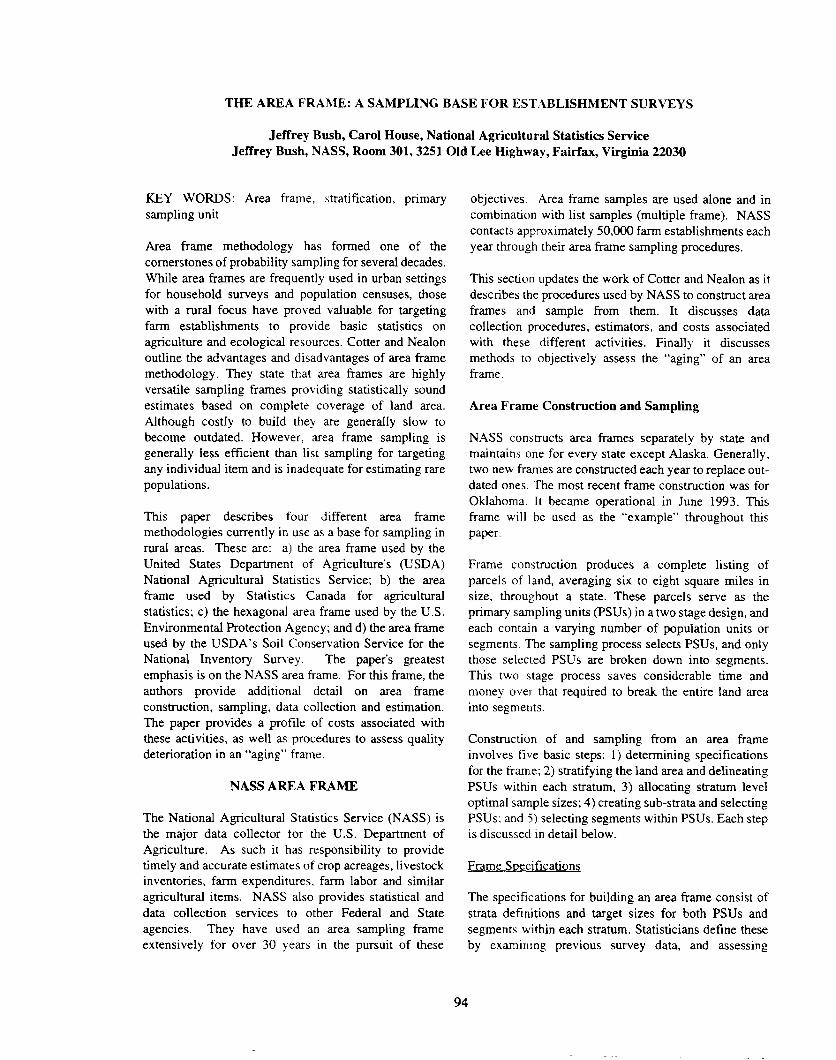
THE AREA FRAME: A SAMPLING BASE FOR ESTABLISHMENT SURVEYS

Jeffrey Bush, Carol House, National Agricultural Statistics ServiceJeffrey Bush, NASS, Room 301, 3251 Old Lee Highway, Fairfax, Virginia 22030

KEY WORDS: Area frame, stratification, primarysampling unit

Area frame methodology has formed one of thecornerstones of probability sampling for several decades.While area frames are frequently used in urban settingsfor household surveys and population censuses, thosewith a rural focus have proved valuable for targetingfarm establishments to provide basic statistics onagriculture and ecological resources. Cotter and Nealonoutline the advantages and disadvantages of area framemethodology. They state that area frames are highlyversatile sampling frames providing statistically soundestimates based on complete coverage of land area.Although costly to build they are generally slow tobecome outdated. However, area frame sampling isgenerally less efficient than list sampling for targetingany individual item and is inadequate for estimating rarepopulations.

This paper describes four different area framemethodologies currently in use as a base for sampling inrural areas. These are: a) the area frame used by theUnited States Department of Agriculture's (USDA)National Agricultural Statistics Service; b) the areaframe used by Statistics Canada for agriculturalstatistics; c) the hexagonal area frame used by the U.S.Environmental Protection Agency; and d) the area frameused by the USDA's Soil Conservation Service for theNational Inventory Survey. The paper's greatestemphasis is on the NASS area frame. For this frame, theauthors provide additional detail on area frameconstruction, sampling, data collection and estimation.The paper provides a profile of costs associated withthese activities, as well as procedures to assess qualitydeterioration in an "aging" frame.

NASS AREA FRAME

The National Agricultural Statistics Service (NASS) isthe major data collector for the U.S. Department ofAgriculture. As such it has responsibility to providetimely and accurate estimates of crop acreages, livestockinventories, farm expenditures. farm labor and similaragricultural items. NASS also provides statistical anddata collection services to other Federal and Stateagencies. They have used an area sampling frameextensively for over 30 years in the pursuit of these

objectives. Area frame samples are used alone and incombination with list samples (multiple frame). NASScontacts approximately 50,000 farm establishments eachyear through their area frame sampling procedures.

This section updates the work of Cotter and Nealon as itdescribes the procedures used by NASS to construct areaframes and sample from them. It discusses datacollection procedures, estimators, and costs associatedwith these different activities. Finally it discussesmethods to objectively assess the "aging" of an areaframe.

Area Frame Construction and Sampling

NASS constructs area frames separately by state andmaintains one for every state except Alaska. Generally,two new frames are constructed each year to replace out-dated ones. The most recent frame construction was forOklahoma. It became operational in June 1993. Thisframe will be used as the "example" throughout thispaper.

Frame construction produces a complete listing ofparcels of land, averaging six to eight square miles insize, throughout a state. These parcels serve as theprimary sampling units (PSUs) in a two stage design. andeach contain a varying number of population units orsegments. The sampling process selects PSUs, and onlythose selected PSUs are broken down into segments.This two stage process saves considerable time andmoney over that required to break the entire land areainto segments.

Construction of and sampling from an area frameinvolves five basic steps: I) determining specificationsfor the frame; 2) stratifying the land area and delineatingPSUs within each stratum, 3) allocating stratum leveloptimal sample sizes; 4) creating sub-strata and selectingPSUs; and 5) selecting segments within PSUs. Each stepis discussed in detail below.

Frame Specifications

The specifications for building an area frame consist ofstrata definitions and target sizes for both PSUs andsegments within each stratum. Statisticians define theseby examining previous survey data, and assessing

94

urbanization and other trends in the state's agriculture.Table 1 lists the frame specifications for the Oklahomaframe.

Strata are based on general land usage. A typical NASSarea frame employs one or more strata for land inintensive agricultural (50 percent or more cultivated),extensive agricultural (15 to 50 percent cultivated), andrange land (less than 15 percent cultivated). Lessfrequently an area frame contains "crop specific" strata.This occurs when a high percentage of the land in a stateis dedicated to the production of a specific type of crop,such as citrus in Florida. In addition, each area frameuses an agri-urban and commercial stratum (more than100 homes per square mile) plus a non-agriculturalstratum including such entities as military bases,airports, and wildlife reserves. Finally, large bodies ofwater are separated into a water stratum.

Boundary points for agricultural strata are generallyrestricted to a set of standardized breaks: 15, 25, 50 and75 percent cultivated. To determine the exact breaks fora given state, the percent cultivated for each segmentsampled under the old frame is calculated from surveydata. The resulting distribution is examined using thecumulative square root of frequency rule proposed byDalenius and Hodges. The standardized breaks may becollapsed or expanded based on the structure of thedistribution.

Stratification and Delineation of PSUs

Once strata definitions are set, the stratification processdivides the land area of the state into PSUs and assignseach to the appropriate land use strata. Each PSU mustconform to the definition and target size outlined for itsparticular stratum. PSU boundaries become a permanentpart of the area frame and must be identifiable for the lifeof the frame. Thus the stratifier uses only the mostpermanent boundaries available when drawing off PSUs.Acceptable boundaries include permanent roads, rivers,and railroads. The final product of the stratificationprocess is a "frame" file which contains a record forevery PSU in a state. Specifically, each record includesthe PSU number, stratum assignment, county, and size.This frame file is maintained over the life of a frame asthe sampling base.

Prior to 1990 the process of stratification used papermaps, aerial photography, satellite imagery, and aconsiderable quantity of skilled labor. The end productwas a frame delineated on paper U.S. Geological Survey1:100,000 scale maps. In 1990, NASS implemented itsComputer Aided Stratification and Sampling System(CASS). CASS automates the stratification steps on agraphical workstation using digital satellite imagery andline graph (road and waterway) data from the U.S.Geological Survey.

Two criteria are the most important for determiningtarget sizes for PSUs and segments within strata:availability of good natural boundaries and the expectednumber of farm establishments. Generally, a lack ofgood boundaries will prompt the use of larger targetsizes, while a large expected number of farmestablishments will prompt smaller target sizes.

The digital satellite imagery employed by the CASSsystem is currently obtained from the thematic mapper(TM) sensor on the LANDSAT-5 satellite. The TM hasa spatial resolution of 30 meters and is made up of 7spectral bands. TM bands 1-5 and 7 reside in thereflective region of the spectrum while band 6 is locatedin the thermal infrared region. NASS experience with theimagery shows that bands 2, 3, and 4 highlight cultivatedareas of land most accurately.

Table 1: Oklahoma Frame Specifications

Primary Sampling Unit SizeSegment

Stratum DefinitionMinimum Desired Maximum Size

(sq. miles) (sq. miles) (sq. miles) (sq. miles)11 >75% CULTIVATED 1.00 6.0 - 8.0 12.0 1.0012 51-75% CULTIVATED 1.00 6.0 - 8.0 12.0 1.0020 15-50% CULTIVATED 1.00 6.0 - 8.0 12.0 1.0031 AGRI-URBAN:>I00 HOMEJSQMI 0.25 1.0 - 2.0 3.0 0.2532 COMMERCIAL:>I00 HOMElSQMI 0.10 0.5 - 1.0 1.0 0.1040 <15% CULTIVATED 3.00 18.0 - 24.0 36.0 3.0050 NON-AGRICULTURAL 1.00 none 50.0 pps·62 WATER 1.00 none none not sampledI. ~e ments are selected with roOaOllJt ro ortlOnalto sIze; I.e. Y:SU S are treatea as se ments.g p y p p

95

g

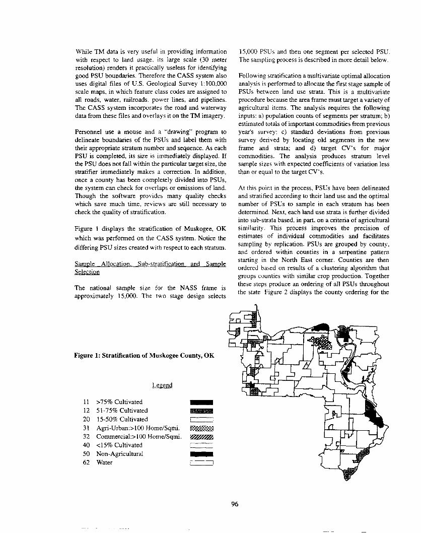
While TM data is very useful in providing informationwith respect to land usage, its large scale (30 meterresolution) renders it practically useless for identifyinggood PSU boundaries. Therefore the CASS system alsouses digital files of U.S. Geological Survey 1:100,000scale maps, in which feature class codes are assigned toall roads, water, railroads. power lines, and pipelines.The CASS system incorporates the road and waterwaydata from these files and overlays it on the TM imagery.

Personnel use a mouse and a "drawing" program todelineate boundaries of the PSUs and label them withtheir appropriate stratum number and sequence. As eachPSU is completed, its size is immediately displayed. Ifthe PSU does not fall within the particular target size, thestratifier immediately makes a correction. In addition,once a county has been completely divided into PSUs,the system can check for overlaps or omissions of land.Though the software provides many quality checkswhich save much time, reviews are still necessary tocheck the quality of stratification.

Figure 1 displays the stratification of Muskogee, OKwhich was performed on the CASS system. Notice thediffering PSU sizes created with respect to each stratum.

Sample Allocation, Sub-stratification and SampleSelection

The national sample size for the NASS frame isapproximately 15,000. The two stage design selects

15,000 PSUs and then one segment per selected PSU.The sampling process is described in more detail below.

Following stratification a multivariate optimal allocationanalysis is performed to allocate the first stage sample ofPSUs between land use strata. This is a multivariateprocedure because the area frame must target a variety ofagricultural items. The analysis requires the followinginputs: a) population counts of segments per stratum; b)estimated totals of important commodities from previousyear's survey: c) standard deviations from previoussurvey derived by locating old segments in the newframe and strata; and d) target CV's for majorcommodities. The analysis produces stratum levelsample sizes with expected coefficients of variation lessthan or equal to the target CV's.

At this point in the process, PSUs have been delineatedand stratified according to their land use and the optimalnumber of PSUs to sample in each stratum has beendetermined. Next, each land use strata is further dividedinto sub-strata based, in part, on a criteria of agriculturalsimilarity. This process improves the precision ofestimates of individual commodities and facilitatessampling by replication. PSUs are grouped by county,and ordered within counties in a serpentine patternstarting in the North East corner. Counties are thenordered based on results of a clustering algorithm thatgroups counties with similar crop production. Togetherthese steps produce an ordering of all PSUs throughoutthe state. Figure 2 displays the county ordering for the

Figure 1: Stratification of Muskogee County, OK

Legend

11 >75% Cultivated12 51-75% Cultivated20 15-50% Cultivated31 Agri-Urban:> 100 Home/Sqmi.32 Commercial:>I00 Home/Sqmi.40 <15% Cultivated50 Non-Agricultural62 Water

~~Hhl

I I

96

state of Oklahoma. Substrata then equally divide theordered PSUs within each stratum, where one PSU isselected per replicate per sub-stratum.

Figure 2: Oklahoma County Ordering

The sampled PSUs in each sub-stratum are randomlyselected with probability proportional to the number ofsegments they contain and are assigned to a replicate. Innon-agricultural and some range strata, where the lack ofsuitable boundaries is a problem, the PSUs themselvesalso serve as segments.

Replicated sampling has several advantages. First itfacilitates sample rotation. Twenty percent of the samplein the NASS frame is rotated each year. Second, it allowsestimation of year to year change from the 80 percent ofthe sample that did not change. Third, it simplifies theprocess of adjusting sample sizes to improve samplingefficiency.

The PSUs selected in the sample selection program arethen located and further broken down into segments. TheCASS system is used for this procedure as well. Just asthe PSUs were originally delineated, so are the segmentswithin each chosen PSU. Segments must be constructedusing permanent boundaries, contain similar amounts ofcultivation, and be equally sized. The CASS systemrandomly chooses one of the segments to sample fromeach PSU.

For data collection, segment boundaries are transferredto large scale NAPP photography. This process iscompleted by hand.

Data CoUection and Estimation

Data Collection

NASS conducts a major area frame survey once eachyear in June. It is called the June Agricultural Survey(JAS). Approximately 15,000 segments are enumeratedand yield approximately 50,000 farm establishments.These segments account for roughly 0.8 percent of the

total land area of the 48 conterminous states. The surveyproduces estimates of crop acreages, grain stocks,number of and land in farms, livestock inventories, farmlabor, and cash receipts at state, regional, and nationallevels. Importantly, the information collected during thissurvey provides a database of information about the farmestablishments sampled through the area frame. Thisinformation is used as a sampling base for follow-onsurveys for the remainder of the year. In particular, farmestablishments are checked against the NASS listsampling frame to measure the incompleteness of thatframe. The follow-on surveys generally use multiple-frame methodology, incorporating list samples with anarea sample which account for this incompleteness.

Prior to the JAS data collection period, newly rotatedsegments along with residential, commercial, and non-agricultural segments are screened for the presence offarm establishments. States implementing a new areaframe must screen all segments. Screening usually takesplace in late April to early May. A questionnaire is filledout for segments which contain no agriculture.

The data collection period for the June AgriculturalSurvey begins June 1 and continues for two weeks.Enumerators conduct face-to-face interviews withoperators of all farm establishments with land inside asegment, and account for all land within the segment.Enumerators are assigned anywhere from 8 to 15segments to survey depending on distance betweensegments and the enumerator's experience level.

Estimation

In the NASS area frame, recall that segments are thepopulation units and the second stage sampling units.The reporting units are the individual farmestablishments within the segments. However,depending on the estimator that is used, these reportingunits are defined somewhat differently. Sometimes theestablishment reports only for its land contained withinthe segment. That part of a segment operated by a singleestablishment is referred to as a "tract." For otherestimators, the establishment reports information for itsentire operation. Other times only farm establishmentswhose operator lives inside the segment reportinformation.

Three different estimators for summarizing area framedata are described below. Each has different advantagesand disadvantages. Each may be used alone to estimateagricultural items, or in conjunction with a list frame toestimate for the undercoverage of that list. Varianceformulations are not presented here in order to conform

97