Survey and GIS Manualfor GPS ( Leica GX1230 )

Second Edition

Anna Kathrin Hodgkinson

1

ContentsPage

Introduction 4

Protocols for Setting up the Leica 1200 GPS 5– A few notes 5

– Survey Book 5– End of survey 5– Weather conditions 5

– Survey Setup 5– Setting up the GPS 5– Creating a new Job 8

– Surveying 11– Start of survey 11– General Survey 12– A rough guide to coding and point IDs 13

Creating points files with co-ordinates and uploading them into the GPS 14

Setting out 16

Troubleshooting on site 18– Survey Errors 18– Problems encountered with the GPS 19

Refreshing the Mobile phone on a Leica RX1250XC GPS using Vodafone 20

How to get the GPS to recognise its mobile phone after it crashed 21

Protocols for downloading the Leica 1200 22

Protocols for inputting data into GIS 28– The Project Manager 28– The data you will deal with 29

– Point and Line data 30– Merging and updating the data 32

Editing Shapefiles 34

Adding Tables / Events Layers to gvSIG 37

Joining tables 40

Printing in gvSIG 42

Georeferencing 45

Problems encountered with gvSIG 50

2

Appendix 1: 51Survey Codelist

Appendix 2: 52Metadata

Appendix 3: 55Drawing of Plans

3

Introduction

The first edition of this manual was produced by Oxford Archaeology North after development of new on-site survey and GIS methodologies applicable to any archaeological project. The second, revised edition was produced in March 2010 after the release of the gvSIG OA Digitial 2010 Edition.It is intended to supply an easy-to-understand but comprehensive guide to survey and GIS, from setting up survey equipment to downloading and processing survey data. It excludes the initial setup of control stations and any preliminary preparation work.

The manual is meant to speed-up, or annihilate the training procedure and provide a guide to survey to field staff in case no professional surveyor is on site. Procedures are explained in great detail with screenshots and photographs where appropriate and guides to troubleshooting and examples for data maintenance are provided. An inexperienced member of field staff should, by following this manual step-by-step, be able to set up a Leica RX1250XC GPS, conduct survey using SmartNet and download and process the survey data, given a certain amount of time. Chapters of this manual have been extracted or adapted from older manuals and adjusted to fit into this guide's sequence and been updated. Any previous authors have been credited.

The present copy of the manual has been adjusted for the use on any site using a Leica RX1250XC GPS without a backpack.

The manual is written in such manner that it can easily be adjusted for individual sites' survey requirements.Chapters can be extracted easily and supplied individually.

Soft- and hardware described in this manual are flexible, although it is recommended to acquire copies of the following:

– gvSIG OADE 2010 - open source GIS softwaredownload from: http://oadigital.net/software/gvsigoade/gvsigoade2010beta

– Inkscape open source vector editing softwaredownload from: http:// www.inkscape.org/

– And a copy of Leica GeoOffice or the equivalent downloading software for the GPS used on site – this should be provided by the manufacturer.

Anna Hodgkinson, the author of this manual, would be grateful for further feedback on its usability, contents and layout. She is employed by OA North as a Supervisor in Geomatics and contactable via email: anna.hodgkinson@thehumanjourney.net

Anna Hodgkinson, March 2010

4

Protocols for Setting up the Leica 1200 GPSby Mark Littlewood and Anne Kilgour Cooper, adapted by Anna Hodgkinson

Any problems, call the Geomatics representative for your project.

A few notes:This equipment is expensive, so please look after it.

Survey Book:It is useful to carry a (yellow and weatherproof) survey book when on site. Write down any queries and errors to be rectified later.

End of survey:– Hit “ESC” a number of times to exit the survey interface and return to the main menu on the

GPS.– Then press and hold “ESC” to turn off the GPS.– Undo all equipment, ensure it is as clean as possible and replace it in the way you received it– Remove the batteries from the GPS and charge them using the Leica charger so everything is

charged for use the following day

Weather conditions:– The GPS is waterproof, but the satellite reception may be bad should the sky be overcast.– After a day out in the rain, the machine must be taken out of the box to dry out, the yellow

cover and the box also need drying out.

Survey SetupSetting up the GPSWhen you collect your equipment make sure that you have the following• 1 pole • a cradle to fix to the pole• a satellite dish with a battery• a computer with battery and Compact Flash (CF) card• 2 spare batteries in the red box• bluetooth mobile phone• a container for the mobile phone• spare mobile phone batteries, a recharger and a car charger

5

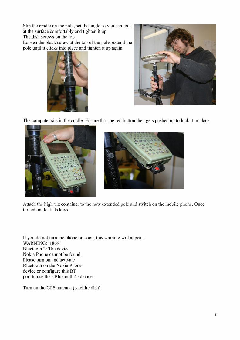
Slip the cradle on the pole, set the angle so you can look at the surface comfortably and tighten it up The dish screws on the top Loosen the black screw at the top of the pole, extend the pole until it clicks into place and tighten it up again

The computer sits in the cradle. Ensure that the red button then gets pushed up to lock it in place.

Attach the high viz container to the now extended pole and switch on the mobile phone. Once turned on, lock its keys.

If you do not turn the phone on soon, this warning will appear:WARNING: 1869Bluetooth 2: The device Nokia Phone cannot be found.Please turn on and activateBluetooth on the Nokia Phonedevice or configure this BTport to use the <Bluetooth2> device.

Turn on the GPS antenna (satellite dish)

6

Press the ON button (bottom right)

Wait for the main screen to load. It will load through a windows CE screen and will eventually get to the main survey screen.

For survey, either press 1, or use the yellow arrow keys and highlight ‘Survey’ and press ENTER (red button).

7

Creating a new Job:On the next screen you will see that the top line is highlighted.

Press enterThis will show a list of jobs available on the machine. You need to start a new one, so press ‘F2’ - New

Type in a sensible job name followed by the date. The job at Brunel Way, Swansea would be Swansea 110207, the job at the Ashmolean, Oxford would be Ashmolean 121206, for example. Ensure sure the job's name can be easily understood by the person downloading and processing the data. The date is VERY IMPORTANT. Press ENTER

Type in a description of the work you are going to do, e.g. Survey Press ENTER

On the creator line, type in your initials.Press ENTER

You will notice near the top of the screen that there are several tabs. The page - F6, button will switch between the different tabs (“Page across”)

Page across to the “Code” tab. Ensure that the codelist the one you were assigned to use on your project. Use the left and right arrows to select the correct one.

Page acrossThe co-ordinate system should be OSGB36 (02)

Page acrossThe average should beAveraging Mode: AverageMethod: WeightedPoints to use: TPS & GPSAvge Limit Pos: 0.050Avge Limit Ht: 0.075

8

press F1 - “Store”

You will return to the list of jobs.Ensure that your job is highlighted and press F1 – Cont

On this page, ensure that the job name is correct, the coord system is correct, the codelist is correctThe “config set” should be SMARTNET ROVERThe antenna should be AX1202 Pole

Press F1 - cont

Look at the very top of the screen. You should see some crosshairs. They will have a large circle, a medium sized circle or a tiny circle around the centre. You should also see an @ symbol to the right of the bit which says how many satellite signals you are getting on the L1 and L2 frequencies. This all means that the GPS has a code only solution with an accuracy of several metres, placing it roughly in the world. The @ symbol means that you are connected to the internet

Press SHIFT followed by F3, which will connect you to the internet and enable your GPS to get an accuracy of up to 15mm.

As before, you will notice a series of tabs showing that there are several pages - “Survey”, “Code”, “Annot”, “Map”

You will mostly be using Code and Map.Page across (F6) to the code page

9

The crosshairs at the very top of the screen will have a large, a medium sized or a small circle around the centre, wait for the circle to become small. Check the numbers at the bottom right of the screen (3D CQ). This will tell you your accuracy. You can’t record points with an accuracy of 0.075m or more.If this accuracy does not get to a reasonable level, ensure you are not standing under a tree, or close to a building. If it is still very inaccurate, check your cables and ensure they are all done up. If it’s still inaccurate, walk around for a few minutes, and if you still don’t get anything, call the emergency contact number you have been provided with.

10

SurveyingStart of survey

General remarks:– If you need to write down a value to check a point before recording it, or for temporary points,

press ‘dist’. Write down the values. Then press ‘rec’ in case you choose to record it.– You can retrieve, edit and delete all data by entering the data menu. This can be found by

pushing the USER button, then selecting “Data manager” (see p. 18).– The data from your current job will be displayed and it will be grouped in points, lines and

areas. The points which make up your lines will be listed as well, but without a code. The ‘Page’ button switches between different bits of information, including a map of what has been surveyed in. You can see what page you’re on by the tabs at the top - Survey, Offset, Code, Map

– The map page is very useful for block planning features. You can zoom in and out and use the yellow arrow keys to scroll around.

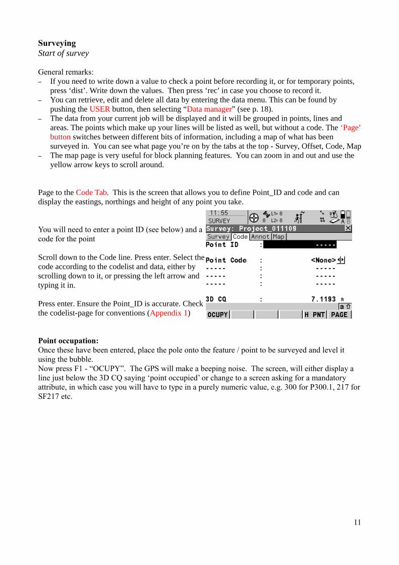
Page to the Code Tab. This is the screen that allows you to define Point_ID and code and can display the eastings, northings and height of any point you take.

You will need to enter a point ID (see below) and a code for the point

Scroll down to the Code line. Press enter. Select the code according to the codelist and data, either by scrolling down to it, or pressing the left arrow and typing it in.

Press enter. Ensure the Point_ID is accurate. Check the codelist-page for conventions (Appendix 1)

Point occupation:Once these have been entered, place the pole onto the feature / point to be surveyed and level it using the bubble. Now press F1 - “OCUPY”. The GPS will make a beeping noise. The screen, will either display a line just below the 3D CQ saying ‘point occupied’ or change to a screen asking for a mandatory attribute, in which case you will have to type in a purely numeric value, e.g. 300 for P300.1, 217 for SF217 etc.

11

General Survey:Points– You need to type in the point ID. See Appendix 1: Codelist – for examples!

– Page to the Code tab.– Use the left and right arrows to select the correct code. – Drawing points and Levels will be surveyed using the

appropriate codes: – An example is given here, but please refer to the

Appendix 1

– Drawing Points for plans: Code: DP P – Point_ID: DP”Plannumber”.1 and DP”Sectionnumber”S for sections etc. See Appendix 2.

– Context (and other) Levels: Code: CTXTLVL – Point_ID: Context number

Lines– NO closed area polygons are surveyed. Use line codes at all times!– Use the left and right arrows to select the correct code. You are able to use the code screen to get

all the codes, and therefore open lines and areas from here. Press cont when you’ve selected the correct code.

– Feature outlines: FEP– Intervention lines: INT– Internal limits of excavation: INT– Limit of excavation: LOE

ALWAYS Press SHIFT + F7 when you’ve finished your line or area.

In the case of errors during survey: see p. 18

12

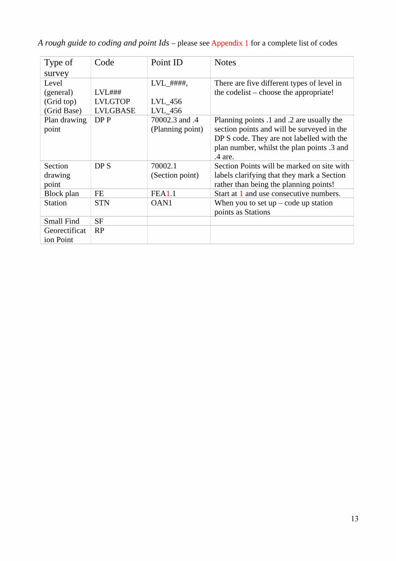
A rough guide to coding and point Ids – please see Appendix 1 for a complete list of codes

Type of survey

Code Point ID Notes

Level (general)(Grid top)(Grid Base)

LVL###LVLGTOPLVLGBASE

LVL_####,

LVL_456 LVL_456

There are five different types of level in the codelist – choose the appropriate!

Plan drawing point

DP P 70002.3 and .4(Planning point)

Planning points .1 and .2 are usually the section points and will be surveyed in the DP S code. They are not labelled with the plan number, whilst the plan points .3 and .4 are.

Section drawing point

DP S 70002.1(Section point)

Section Points will be marked on site with labels clarifying that they mark a Section rather than being the planning points!

Block plan FE FEA1.1 Start at 1 and use consecutive numbers. Station STN OAN1 When you to set up – code up station

points as StationsSmall Find SFGeorectification Point

RP

13

Creating points files with co-ordinates and uploading them into the GPS

You may be asked to set out points from known co-ordinates on site. The points should exist as a shapefile in your GIS project.Ensure each point has an individual point ID.Ensure you have the X and Y information within the shapefile's .dbf file. You can apply this manually by using the field calculator:

Start editing the shapefile containing the information of the points you wish to set out and open its attrubute table. Now select: “Table – Manage Fields” and add two columns named “Eastings” and “Northings”. Choose “Double” as data type. - two new columns will appear in the attribute table. Click on the “Eastings” column and open the “Field calculator” toolHighlight the “Eastings” column on the left hand side, and on the right, scroll down until you find “x”. Double click only on “x” and confirmthis.

Repeat the above for the “Northings” column, selecting “y” in the field calculator.

The shapefile's .dbf file now contains Eastings and Northings, i.e. X and Y data.

Open the .dbf file from its stored location (right-click on the shapefile in gvSIG and select “properties” - the filepath will help locating the .dbf file). Save the file as a .csv (comma delimited) file in a logical location.

Now plug the CF card into the computer and navigate to its “Data” folder. Paste a copy of the .csv file into this “Data” folder.

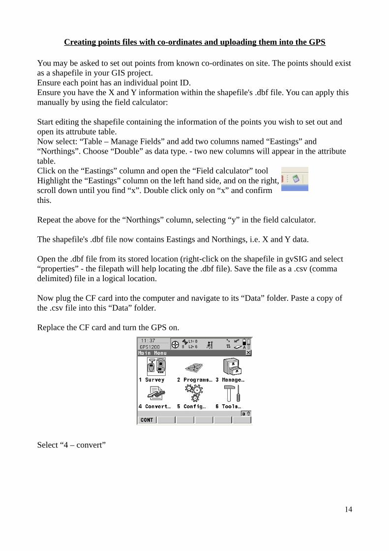
Replace the CF card and turn the GPS on.

Select “4 – convert”

14

Select “2 – Import ASCII/GSI Data to Job”

Select:Import: ASCII DataFolder: the Data folder on the CF cardFrom File: the .csv file you uploaded onto the card earlierTo job: The job you wish to use as your setting out job – create a new, empty job, called “STKE_(with a reference to what is being set out)”Header: “1” (The .dbf file has a header, therefore you have to specify that row 1 of the .csv file contains the information, rather than standing for its own point)

Hit “CONT” and a message will be displayed, informing you that the points have been imported.

15

Setting out

You may be asked to set out new points created in GIS or retrieve previously surveyed points. In any case, the co-ordinates of the points to be staked out must be known and stored on the GPS.For uploading points created from a shapefile, see p. 14.

Make a list and sketch-map of the points to be staked out for orientation and take this to site.

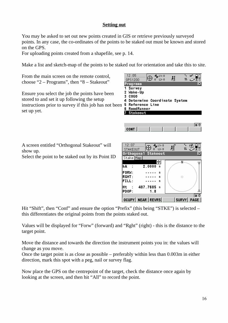
From the main screen on the remote control, choose “2 – Programs”, then “8 – Stakeout”

Ensure you select the job the points have been stored to and set it up following the setup instructions prior to survey if this job has not been set up yet.

A screen entitled “Orthogonal Stakeout” will show up. Select the point to be staked out by its Point ID

Hit “Shift”, then “Conf” and ensure the option “Prefix” (this being “STKE”) is selected – this differentiates the original points from the points staked out.

Values will be displayed for “Forw” (forward) and “Rght” (right) - this is the distance to the target point.

Move the distance and towards the direction the instrument points you in: the values will change as you move.Once the target point is as close as possible – preferably within less than 0.003m in either direction, mark this spot with a peg, nail or survey flag.

Now place the GPS on the centrepoint of the target, check the distance once again by looking at the screen, and then hit “All” to record the point.

16

If you now check the Data Manager, the point just recorded will show up as “STKE##” and the point initially selected as a target will show up with a small flag next to it.

The STKE points will be surveyed without a code – use the data manager to change this manually.

Write the number on the tags in a white space and make people aware of them.

17

Troubleshooting on site

Survey ErrorsErrors can be corrected on site, or in the office, so make sure all errors are clearly written in the survey book.

To correct mistakes while you’re surveying, press Userand then Data Manager

Highlight the point and press “edit”.You can change the Point ID, code and reflector height. Each reflector height must be done separately, so if there’s ten in a row, you’ll have to do all ten.Once it’s altered, press storeTo change lines, page to the lines tab.Select the line and press enter. You can remove points surveyed in by mistake. N.B. These will be downloaded as a NOCODEPOINT shapefile, but saved only as separate points.

Once you’re done, press cont.

Otherwise, write down your errors on your survey sheet and ensure the person who is dealing with the download knows about them. It may be quicker to correct in LGO or gvSIG.

18

Problems encountered with the GPS:

Problems with coding:

In case the codelist shows only point- or only linecodes when coding up:

– From the Main Menu select “3 Management”– Select “5 Configuration Sets”– Highlight the appropriate one and hit “EDIT”– A Wizard screen is displayed – press “CONT” (F1) until you reach a page entitled “Coding

and Linework”On this screen highlight the lign reading: “Show Codes:” and ensure that “All Codes” is selected (rather than only point- or line codes).

19

Refreshing the Mobile phone on a Leica RX1250XC GPS using Vodafone by Mark Littlewood

It is uncertain how successful these methods are or whether they will work with a backpack GPS. In places like Kent and/or Essex you may find your 3D coordinate quality dropping quite alarmingly around lunchtime and in the late afternoon/evening. This will be despite the fact that you are tracking plenty of satellites and the fact that your phone has a good signal. Basically Packet Data is an added extra on the Vodafone network and Smartnet GPS use this extra bandwidth to work in. However mobile phone calls have priority and when there are a lot of people on the system, a GPS will get pushed down the queue. There are two suggested methods for refreshing your place in the queue and getting your 3D coordinate quality back.

Network change

On your mobilephone (Nokia 6021):

Menu-Settings-Phone settings-Operator selection

Switch from Automatic to Manual

Select another network.

Repeat:

Menu-Settings-Phone settings-Operator selection

Switch from Automatic to Manual

and this time select the Vodafone network

Repeat

Menu-Settings-Phone settings-Operator selection

and select Automatic

This should clear the Vodaphone queue and put you back in your original queue position. 3D coordinate quality should return.

Hard e-set

With the GPS switched on;– Remove the battery– Remove the SIM card– Replace the battery– Switch back on– Remove the battery – Replace the battery back in– Replace the Sim card

This should also refresh your place in the queue.

20

How to get the GPS to recognise its mobile phone after it crashedby Mark Littlewood

Shift+F5

Now utilising red stylus pen:

Windows flag in bottom left hand corner/settings/control panel

Bluetooth Device Properties in upper left corner (double click)

Should have 2 devices in the Trusted bit. One will be the saucer shaped antenna called [ Unnamed (0012f3051455)

The other will be your phone. Highlight it/arrow at bottom of screen pointing to the untrusted box click on. Tap 0k then the cross in the top.

Cross again.

Double click SmartWorx symbol to get back to Main Menu

Choose your configuration setting then you'll probably have to go to:

5 Config.../ 4 Interfaces/

Find the Internet line F3 EDIT then F4 SRCH.

It should find your phone whereby you may have to put the pin number onto both machines again 1234 ( or 0000). Basically PIN number has to be the same on both machines. Otherwise you will have to do all of the above. Should you ever need to search for the GPS antenna the pin code to tap in is always 0000.

21

Protocols for downloading the Leica 1200by Anne Kilgour Cooper, adapted by Anna Hodgkinson

– Navigate to Project\Survey\dated folders\Survey2009\

– Copy the folder called GPS_DATE_Template and paste it into the same folder. Rename it with the date of your survey job. (Project_TST_######)

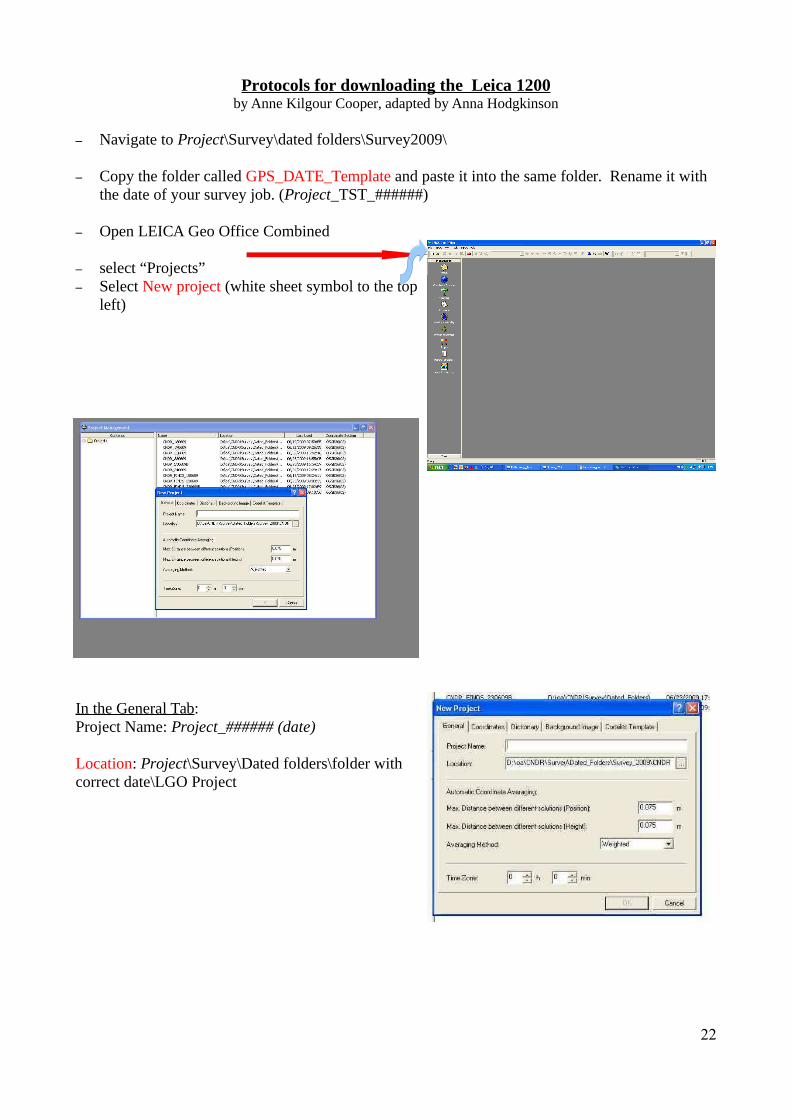
– Open LEICA Geo Office Combined

– select “Projects”– Select New project (white sheet symbol to the top

left)

In the General Tab:Project Name: Project_###### (date)

Location: Project\Survey\Dated folders\folder with correct date\LGO Project

22

Coordinates Tab:Coordinate system: OSGB36

Codelist_Template: Leica System 1200 – Advanced

Hit “OK”

Now you need to import the raw data.

Ensure that the card is in the card reader.Usually the CF card will have to go straight back into the GPS on site to ensure survey coverage. Therefore it is advisable to copy the data from CF card\DBX to a folder on the PC (e.g. Temporary_Survey_Download on the desktop). Copy all the files with the job's name to this folder.

Go to Import - Raw data or hit the equivalent button on the toolbar.

Locate to the CF card\DBX\the project you want to import or to the folder on the PC containing the the raw data copied across earlier (Temporary_Survey_Download on the desktop)

Click import.

23

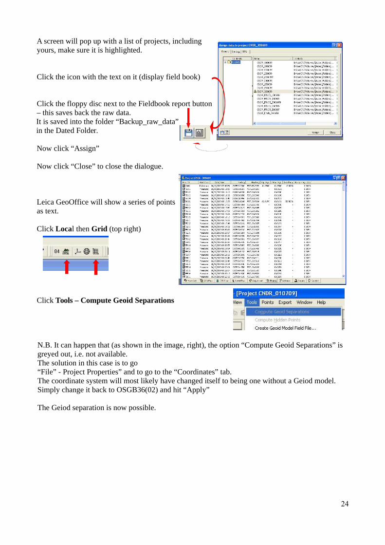
A screen will pop up with a list of projects, includingyours, make sure it is highlighted.

Click the icon with the text on it (display field book)

Click the floppy disc next to the Fieldbook report button – this saves back the raw data. It is saved into the folder “Backup_raw_data” in the Dated Folder.

Now click “Assign”

Now click “Close” to close the dialogue.

Leica GeoOffice will show a series of points as text.

Click Local then Grid (top right)

Click Tools – Compute Geoid Separations

N.B. It can happen that (as shown in the image, right), the option “Compute Geoid Separations” is greyed out, i.e. not available. The solution in this case is to go “File” - Project Properties” and to go to the “Coordinates” tab.The coordinate system will most likely have changed itself to being one without a Geiod model. Simply change it back to OSGB36(02) and hit “Apply”

The Geiod separation is now possible.

24

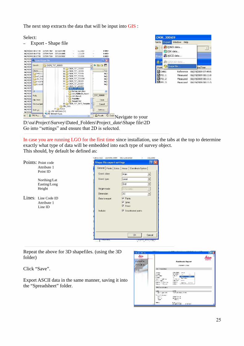
The next step extracts the data that will be input into GIS :

Select:– Export - Shape file

Navigate to your D:\oa\Project\Survey\Dated_Folders\Project_date\Shape file\2DGo into “settings” and ensure that 2D is selected.

In case you are running LGO for the first time since installation, use the tabs at the top to determine exactly what type of data will be embedded into each type of survey object. This should, by default be defined as:

Points: Point codeAttribute 1Point ID

Northing/LatEasting/LongHeight

Lines: Line Code IDAttribute 1Line ID

Repeat the above for 3D shapefiles. (using the 3D folder)

Click “Save”.

Export ASCII data in the same manner, saving it into the “Spreadsheet” folder.

25

Now right click on the fieldbook report in Leica GeoOffice and print it as a PDF using the PDFCreator. It will be called the same as the job and save it in your dated folder\LGO_Fieldbook_Report.

Ensure you name each saved item (or group of items in the case of shapefiles) with the name of the job and save it in the dated folder/appropriate folder!!!

Please ensure you name everything appropriately and in the same way as the previous survey!

Close Leica Geo Office.

26

Protocols for inputting data into GISby Anna Hodgkinson

with extracts from Ducke, B. 2008, “An Introduction to gvSIG Open Source GIS on Windows”

The GIS software package used is called gvSIG. It is an open source program developed by the Government of Valencia, Spain. The particular package we use is the OA Digital 2010 Edition, based on gvSIG 1.10, adapted by Ben Ducke.

The following instructions are based on the assumption that the user is operating a Microsoft Windows computer.

– Open the current gvSIG project, usually stored in D:\Project\GIS\projects\gvSIG

– Open the project by double-clicking – gvSIG opens

– If no map is displayed go “Show – Project Manager”

The Project Manager

– The Project Manager provides a way of working with several data views and map layouts within one project. It contains the sections “View”, “Table” and “Map”.

– You will need to get back to the project manager often. To do so, choose “Window - Project manager” from the main menu.

– Select “View” and highlight the view you wish to see - click “open”: The view will be displayed.

27

– The view usually contains all the relevant data from the present fieldwork.

– The data is displayed in layers, which are saved as shapefiles and referenced externally:

– Highlight (by clicking onto) one of the layers and right-click. Select “Properties”: This will show you, amongst other information, the filepath that this file is stored at.

– The filepath for all the current layers in the GIS project are stored in Project\GIS\shapefiles\current!

– ONLY the current layers can be stored here, the old ones are to be removed to the folder Project\GIS\shapefiles\old as soon as the update has been undertaken

– The file may be listed under a different name in gvSIG – this is because it is possible to rename the individual layers once they have been imported into GIS:

“Archaeological Features is the layer name, whilst the shapefile is called “Arch_features_240609”

The tabs at the top of the “Properties” Window give the options to change a particular layer's appearance in the “Symbology” tab and also to display attribute data in the “Labelling“ tab.

28

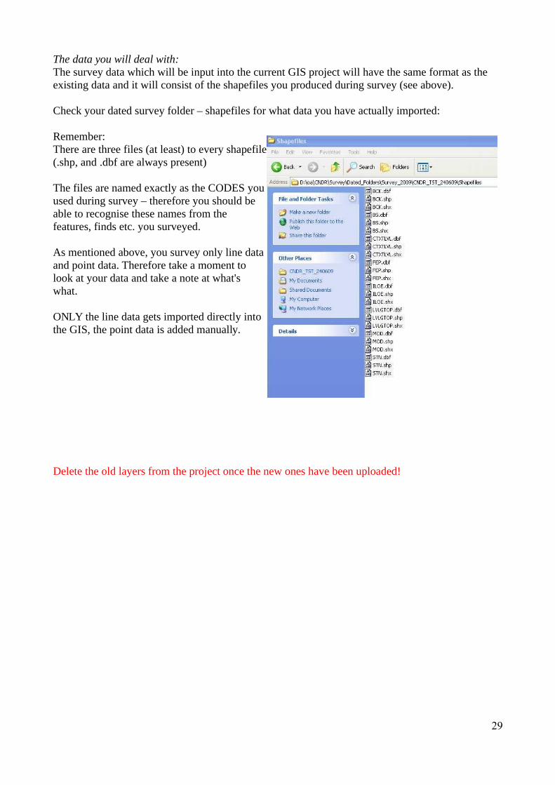
The data you will deal with:The survey data which will be input into the current GIS project will have the same format as the existing data and it will consist of the shapefiles you produced during survey (see above).

Check your dated survey folder – shapefiles for what data you have actually imported:

Remember: There are three files (at least) to every shapefile (.shp, and .dbf are always present)

The files are named exactly as the CODES you used during survey – therefore you should be able to recognise these names from the features, finds etc. you surveyed.

As mentioned above, you survey only line data and point data. Therefore take a moment to look at your data and take a note at what's what.

ONLY the line data gets imported directly into the GIS, the point data is added manually.

Delete the old layers from the project once the new ones have been uploaded!

29

Point and Line data: Open the main view of the gvSIG project (unless, of course, it is already open).

The codes used for this have a description each: eg. ILOE = Internal Limit of excavation, relating to a layer in the GIS project (see Appendix 2).Your survey data will (probably) include archaeological features. These will be on the “FEP” code in the GPS, therefore downloaded into your dated shapefiles folder as “FEP” and the GIS project will include a layer called “Archaeological_features_110609” (the shapefile is dated).The date does not have to be that of the previous day – it depends on whether any archaeological features were surveyed that day or not.

The following point-shapefiles from your survey folder will not be included in the update and do not need to be updated:– STN – as these remain constant– BCK – is for reference only in case the survey data looks wrong after it has been imported into

GIS (in which case import the BCK point – one should be taken at for each survey setup – and check whether it is in the same location as your backsight-point)

– NOCODEPOINT: open the .dbf file of the NOCODEPOINT shapefile and check whether it contains any finds or other point data you might have forgotten to code up. Open the file with scalc (OpenOffice Spreadsheet), NOT with Microsoft Excel!! If you surveyed following the above instructions, you should have no data on wrong layers!!!

Now: add the fresh survey data.Shapefiles are imported ONE AT A TIME and dealt with separately to avoid errors!!!

Choose “View - Add layer” from the main menu or click on the layer icon in the icon bar.

The “Add layer” dialogue will pop up.

Make sure the “File” tab is selected and choose “Add”.

30

Ensure the option “Shapefile” is selected.

Navigate to D:\oa\Project\Survey\Dated_Folders\Survey_2009\Project_TST_DATE\shapefiles\2D and select one line layer.Then click “OK”. The shapefile will now be added to the layer list of the active view.

If you cannot see anything: Use “zoom to layer” from the layer context menu (right mouse button) to zoom to the extents of a specific layer .

31

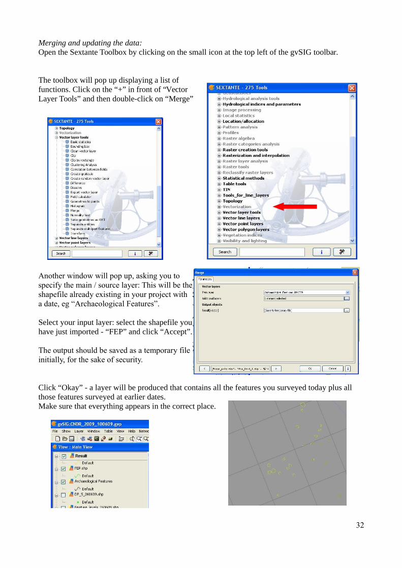
Merging and updating the data:Open the Sextante Toolbox by clicking on the small icon at the top left of the gvSIG toolbar.

The toolbox will pop up displaying a list of functions. Click on the “+” in front of “Vector Layer Tools” and then double-click on “Merge”

Another window will pop up, asking you to specify the main / source layer: This will be the shapefile already existing in your project with a date, eg “Archaeological Features”.

Select your input layer: select the shapefile you have just imported - “FEP” and click “Accept”.

The output should be saved as a temporary file initially, for the sake of security.

Click “Okay” - a layer will be produced that contains all the features you surveyed today plus all those features surveyed at earlier dates.Make sure that everything appears in the correct place.

32

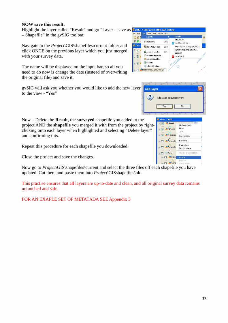
NOW save this result: Highlight the layer called “Result” and go “Layer – save as – Shapefile” in the gvSIG toolbar.

Navigate to the Project\GIS\shapefiles\current folder and click ONCE on the previous layer which you just merged with your survey data.

The name will be displayed on the input bar, so all you need to do now is change the date (instead of overwriting the original file) and save it.

gvSIG will ask you whether you would like to add the new layer to the view - “Yes”

Now – Delete the Result, the surveyed shapefile you added to the project AND the shapefile you merged it with from the project by right-clicking onto each layer when highlighted and selecting “Delete layer” and confirming this.

Repeat this procedure for each shapefile you downloaded.

Close the project and save the changes.

Now go to Project\GIS\shapefiles\current and select the three files off each shapefile you have updated. Cut them and paste them into Project\GISshapefiles\old

This practise ensures that all layers are up-to-date and clean, and all original survey data remains untouched and safe.

FOR AN EXAPLE SET OF METATADA SEE Appendix 3

33

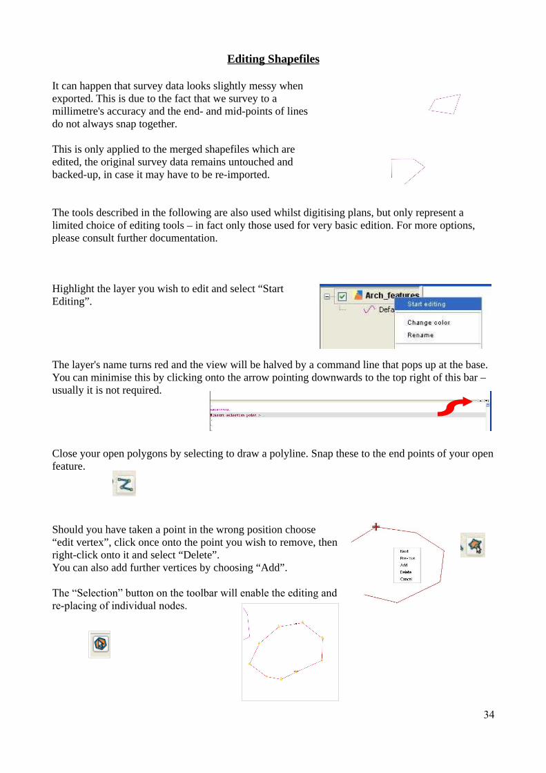
Editing Shapefiles

It can happen that survey data looks slightly messy when exported. This is due to the fact that we survey to a millimetre's accuracy and the end- and mid-points of lines do not always snap together.

This is only applied to the merged shapefiles which are edited, the original survey data remains untouched and backed-up, in case it may have to be re-imported.

The tools described in the following are also used whilst digitising plans, but only represent a limited choice of editing tools – in fact only those used for very basic edition. For more options, please consult further documentation.

Highlight the layer you wish to edit and select “Start Editing”.

The layer's name turns red and the view will be halved by a command line that pops up at the base. You can minimise this by clicking onto the arrow pointing downwards to the top right of this bar – usually it is not required.

Close your open polygons by selecting to draw a polyline. Snap these to the end points of your open feature.

Should you have taken a point in the wrong position choose “edit vertex”, click once onto the point you wish to remove, then right-click onto it and select “Delete”.You can also add further vertices by choosing “Add”.

The “Selection” button on the toolbar will enable the editing and re-placing of individual nodes.

34

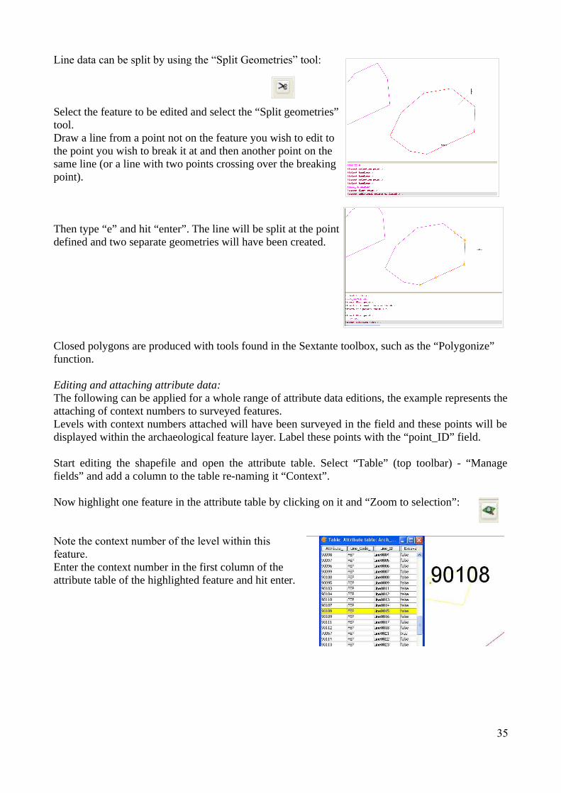
Line data can be split by using the “Split Geometries” tool:

Select the feature to be edited and select the “Split geometries” tool. Draw a line from a point not on the feature you wish to edit to the point you wish to break it at and then another point on the same line (or a line with two points crossing over the breaking point).

Then type “e” and hit “enter”. The line will be split at the point defined and two separate geometries will have been created.

Closed polygons are produced with tools found in the Sextante toolbox, such as the “Polygonize” function.

Editing and attaching attribute data:The following can be applied for a whole range of attribute data editions, the example represents the attaching of context numbers to surveyed features. Levels with context numbers attached will have been surveyed in the field and these points will be displayed within the archaeological feature layer. Label these points with the “point_ID” field.

Start editing the shapefile and open the attribute table. Select “Table” (top toolbar) - “Manage fields” and add a column to the table re-naming it “Context”.

Now highlight one feature in the attribute table by clicking on it and “Zoom to selection”:

Note the context number of the level within this feature.Enter the context number in the first column of the attribute table of the highlighted feature and hit enter.

35

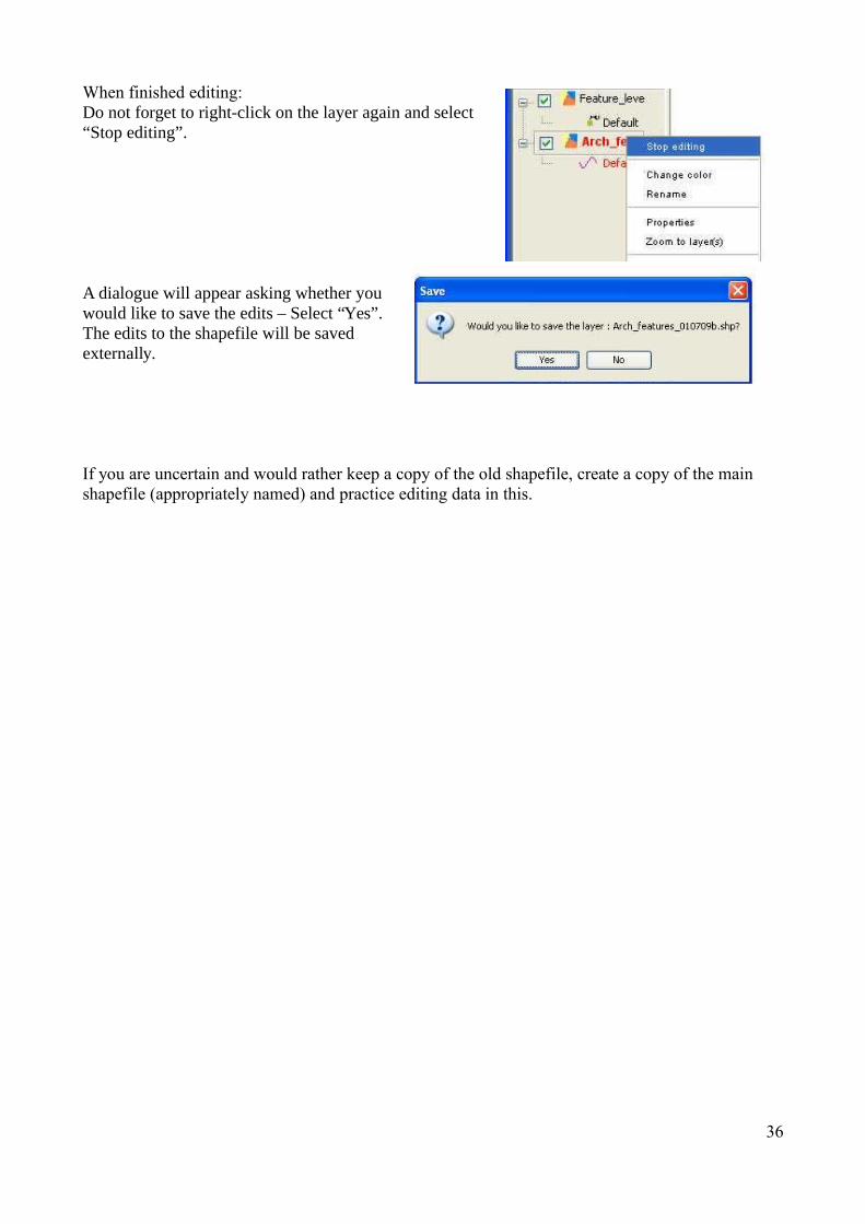
When finished editing:Do not forget to right-click on the layer again and select “Stop editing”.

A dialogue will appear asking whether you would like to save the edits – Select “Yes”. The edits to the shapefile will be saved externally.

If you are uncertain and would rather keep a copy of the old shapefile, create a copy of the main shapefile (appropriately named) and practice editing data in this.

36

Adding Tables / Events Layers to gvSIGThis methodology describes how to create tables of points with known co-ordinates and how to load them into gvSIG. It is for example useful for merging existing points shapefiles with additional surveyed ones, or for creating lists of points for reference.

The described sequence deals with the merging of new survey data with the main datasets after two different types of survey equipment were used on site and the data could no longer be merged using the Sextante Toolbox in gvSIG. It is, nevertheless, applicable to a broad range of data management methodologies.

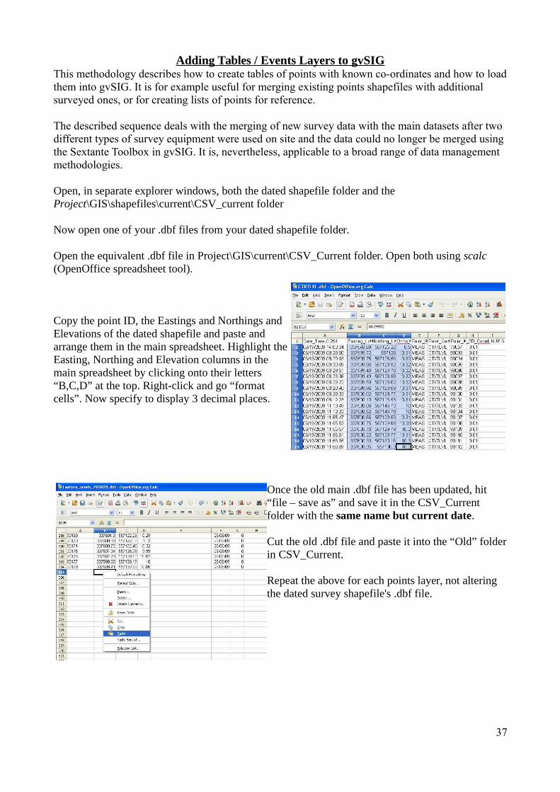
Open, in separate explorer windows, both the dated shapefile folder and the Project\GIS\shapefiles\current\CSV_current folder

Now open one of your .dbf files from your dated shapefile folder.

Open the equivalent .dbf file in Project\GIS\current\CSV_Current folder. Open both using scalc (OpenOffice spreadsheet tool).

Copy the point ID, the Eastings and Northings and Elevations of the dated shapefile and paste and arrange them in the main spreadsheet. Highlight the Easting, Northing and Elevation columns in the main spreadsheet by clicking onto their letters “B,C,D” at the top. Right-click and go “format cells”. Now specify to display 3 decimal places.

Once the old main .dbf file has been updated, hit “file – save as” and save it in the CSV_Current folder with the same name but current date.

Cut the old .dbf file and paste it into the “Old” folder in CSV_Current.

Repeat the above for each points layer, not altering the dated survey shapefile's .dbf file.

37

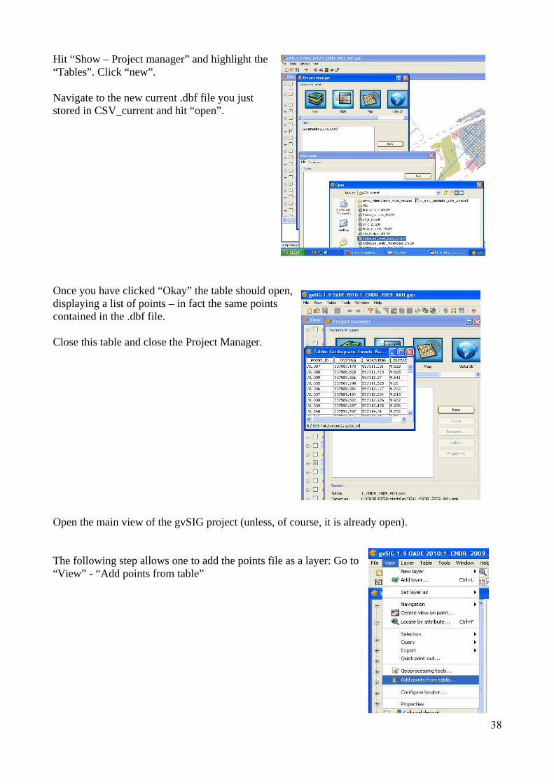
Hit “Show – Project manager” and highlight the “Tables”. Click “new”.

Navigate to the new current .dbf file you just stored in CSV_current and hit “open”.

Once you have clicked “Okay” the table should open, displaying a list of points – in fact the same points contained in the .dbf file.

Close this table and close the Project Manager.

Open the main view of the gvSIG project (unless, of course, it is already open).

The following step allows one to add the points file as a layer: Go to “View” - “Add points from table”

38

Now select the table you just added to the project from the drop-down menu.Define “Easting” and “Northing” as input locators and hit “OK”The points contained in the data-table will be displayed as a layer in gvSIG

Activate this function and select the table you just added to the project from the dropdown menu.Define “Easting” and “Northing” as input locators and hit “OK”The points contained in the data-table will be displayed as a layer in gvSIG

Now save this data as a shapefile:– Highlight the layer created which ends in “.dbf” and go “Layer – save as – Shapefile” in the

gvSIG toolbar– Navigate to the Project\GIS\shapefiles\current folder and click ONCE on the previous layer– Change the date (instead of overwriting the original file) and save it. – gvSIG will ask you whether you would like to add the new layer to the view - “Yes”– Now – Delete the old complete shapefile AND the .dbf layer from the project by right-clicking

onto each layer when highlighted and selecting “Delete layer” and confirming this.

– Now go to Project\GIS\shapefiles\current and select the three files off each shapefile you have updated. Cut them and paste them into Project\GISshapefiles\old

39

Joining tables

The following description is based on data tables exported from a MS Access database and therefore the exporting procedure forms the first part of this chapter. It is, however, possible, to link any .dbf file to a layer file in gvSIG, as long asa) they share a common field usable as a linking field, such as a key andb) this common field is of exactly the same data type in both tables.

Exporting the data-table from MS Access– Open the MS Access database and the table you wish to join with a layer in gvSIG.– Do “File – Save as/Export” to export this table as an XLS (3) file. Save it and then open the

XLS file (in either OpenOffice or MS Excel) and save it as a DBase (.dbf) file.

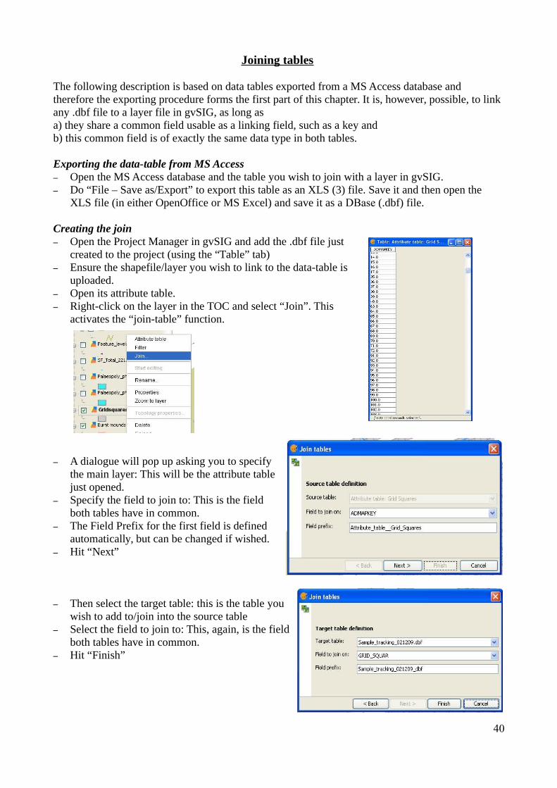
Creating the join– Open the Project Manager in gvSIG and add the .dbf file just

created to the project (using the “Table” tab)– Ensure the shapefile/layer you wish to link to the data-table is

uploaded.– Open its attribute table. – Right-click on the layer in the TOC and select “Join”. This

activates the “join-table” function.

– A dialogue will pop up asking you to specify the main layer: This will be the attribute table just opened.

– Specify the field to join to: This is the field both tables have in common.

– The Field Prefix for the first field is defined automatically, but can be changed if wished.

– Hit “Next”

– Then select the target table: this is the table you wish to add to/join into the source table

– Select the field to join to: This, again, is the field both tables have in common.

– Hit “Finish”

40

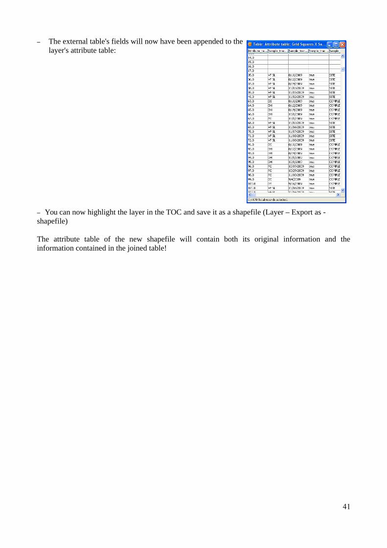
– The external table's fields will now have been appended to the layer's attribute table:

– You can now highlight the layer in the TOC and save it as a shapefile (Layer – Export as - shapefile)

The attribute table of the new shapefile will contain both its original information and the information contained in the joined table!

41

Printing in gvSIG

Open the Project manager, and click on “Map” - A list of printable maps will be displayed

Now either– highlight an existing map and click “open” or– click “new”, then highlight the new map at the bottom of the list and click “open”

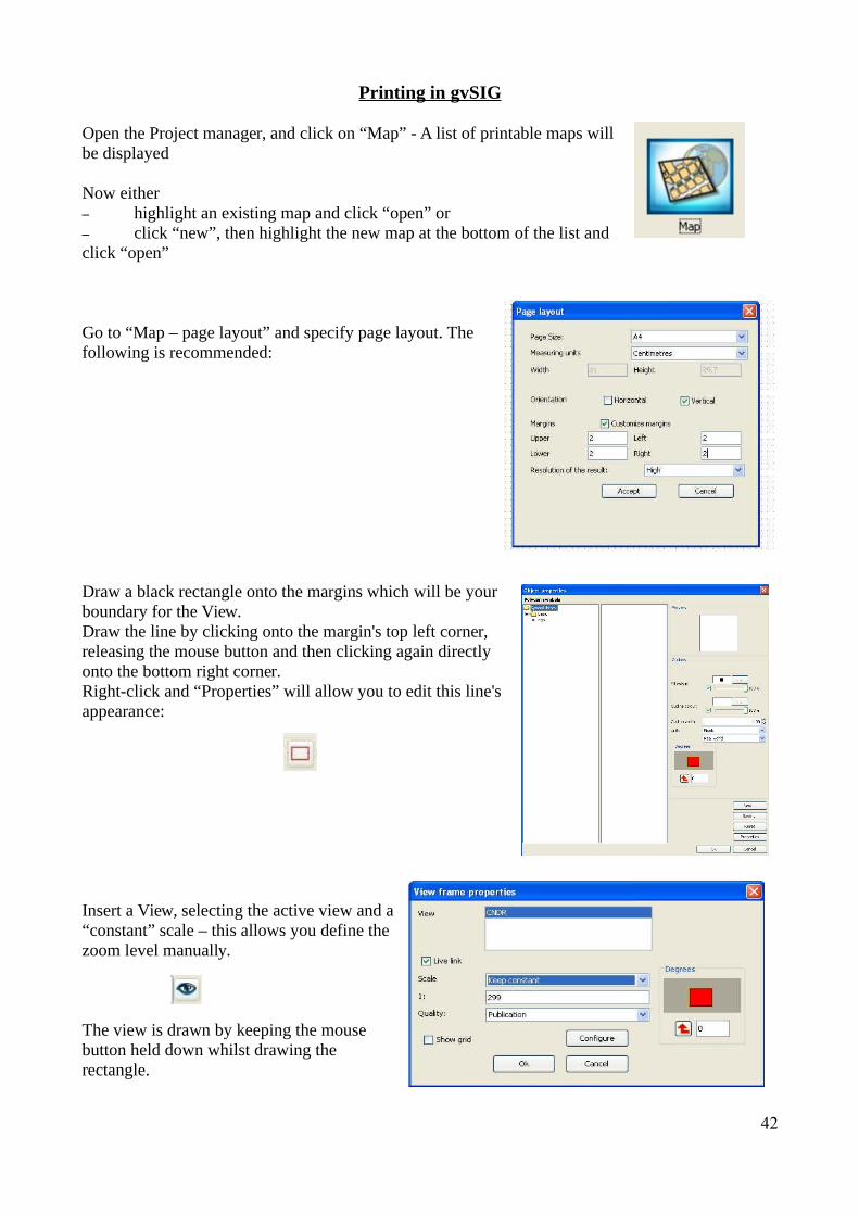
Go to “Map – page layout” and specify page layout. The following is recommended:

Draw a black rectangle onto the margins which will be your boundary for the View. Draw the line by clicking onto the margin's top left corner, releasing the mouse button and then clicking again directly onto the bottom right corner.Right-click and “Properties” will allow you to edit this line's appearance:

Insert a View, selecting the active view and a “constant” scale – this allows you define the zoom level manually.

The view is drawn by keeping the mouse button held down whilst drawing the rectangle.

42

Once the view has been inserted, right-click onto it and move it to the bottom of the map – the line previously drawn will re-appear.

Insert a scalebar and edit its properties. This can sometimes be a little temperamental in gvSIG and requires some patience:

Insert a North Arrow:OA employees: use the OA North Arrow specified by a blank space in the list of North Arrows.

Insert a legend:

43

A dialogue will pop up, allowing you to choose from layers you wish to name in the legend – Generally everything shown on the map should be in the legend. You will have to highlight the active view in order to activate the list of options. The key will generate layer names according to what they are called in the main view – therefore it is sensible to name them appropriately in the TOC before opening the map (right-click – “Rename”).

Draw white rectangles (white fill without transparency) for the Scalebar, North Arrow and Legend if they are on a multicoloured background.

Print your map as a PDF – save in Project\GIS\Daily_PDF\ - make a dated folder and name your map appropriately.

If the map is meant to be included into a report or supposed to serve any other official purpose, the open source vector editing software Inkscape is highly useful for editing of PDFs: – Open the .pdf file in Inkscape– Then select everything by hitting “ctrl” + “A”– Go: “Object” - “Ungroup” - repeat this until everything has been ungrouped: Objects can be moved individually– Ensure to separate the numbers from the scalebar!– Draw white rectangles over the margins and arrange items in an appropriate order

(“Object” - “Raise” or “Lower”), so that overlapping items are not printed in the margins– Save the drawing as both .svg and .pdf!

A detailed guide to producing layouts in Inkscape is also available on www.openarchaeology.net.

44

Georeferencing

These instructions apply to georectified photography and plans drawn on site, which have to be georeferenced prior to digitising.

General notes: • When placing survey target tags in the ground, ensure not to pierce the tag in the centre of

the target, but secure it on both sides, leaving the centre of the target, the cross-hairs, clear and accurate. Furthermore, each photograph requires at least four targets placed at the same level, evenly spaced and the photograph must be taken as vertically as possible.

• It is better to use more points rather than less for each georectification in order to achieve the highest level of flexibility and accuracy. The RMS error displayed during the process of georefencing is an indication of control point placement consistency, *not* the quality of the rectification itself. The georectification should be accurate enough as long as the RMS does not get higher than the required accuracy, (e.g. 0.05 for 5cm). 3 is the minimum for the rectification to actually work, and ideally, control points should be distributed evenly throughout the image. For images that have significant internal "warping" (e.g. old scanned maps, photos of very "curvy" surfaces), at least 7 points should be used.The formula for figuring out the minimum number of control points for a selected order "n" of transformation is: ((n + 1) * (n + 2) / 2) – So 1st order = 3, 2nd order = 6

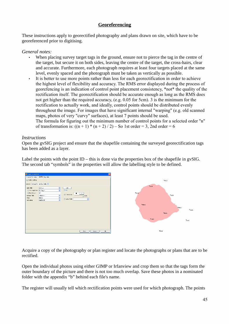
InstructionsOpen the gvSIG project and ensure that the shapefile containing the surveyed georectification tags has been added as a layer.

Label the points with the point ID – this is done via the properties box of the shapefile in gvSIG. The second tab “symbols” in the properties will allow the labelling style to be defined.

Acquire a copy of the photography or plan register and locate the photographs or plans that are to be rectified.

Open the individual photos using either GIMP or Irfanview and crop them so that the tags form the outer boundary of the picture and there is not too much overlap. Save these photos in a nominated folder with the appendix “b” behind each file's name.

The register will usually tell which rectification points were used for which photograph. The points

45

used for planning should be obvious from the plan where drawing- or gridpoints should have been labelled.Normally several shots will be taken per view, which will also be logged in the register, but it will have to be decided which photograph is of the highest quality to be used.

The following uses georectified photography as an example, but is just as applicable to plans:

The “Georeferencer” tool in gvSIG is used to place the pictures. This is activated by selecting “Tools - Georeferencing”

This window will pop up:

Background layers: Select the active view

Input file:Select the image you wish to georeference.

Output file:Can be identified, but if nothing is chosen, the metadata is attached to the Input file.

Transformation: Affine is the most commonly used transformation and requires a minimum of three control points. Refer to the text below “General notes” at the start of this chapter for further information on transformations.

Hit “Accept” and the following screen will appear:The active view will appear in the left window, zoomed to its full extent, whilst the right window shows the file to be georeferenced. The red crosshairs centre onto a zoomed view of either window, appearing at the base.

46

The “Settings” tool will allow you to change several settings, such as background colours and transformations:

A black background is not always a convenient working background, especially as labels are often displayed in black and thus not legible

47

Using • The information on the photography register,• the existing survey data,• any previously georeferenced photographs of the same area and• one's knowledge of the site,

familiarise yourself with the points on the ground and in the image. Be sure to know the image's rotation and orientation.

Then select the first set of points and use the “Zoom to select area” tool to zoom into the first source and target points in both windows.

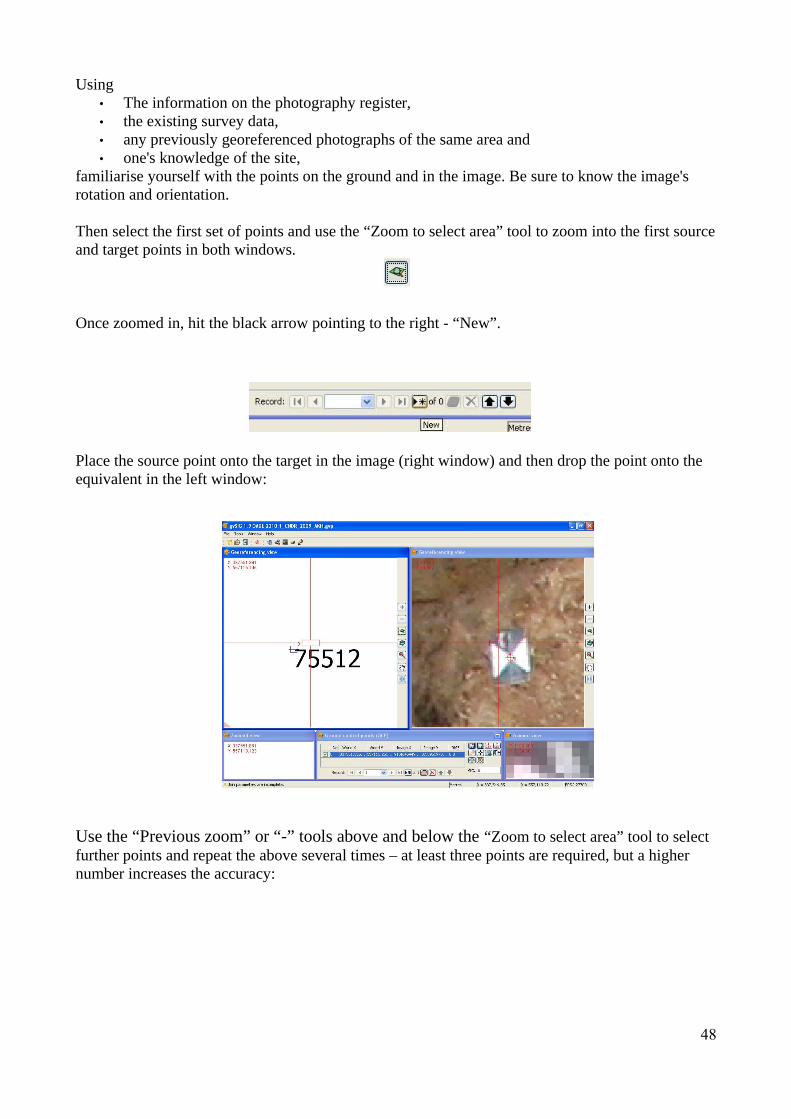
Once zoomed in, hit the black arrow pointing to the right - “New”.

Place the source point onto the target in the image (right window) and then drop the point onto the equivalent in the left window:

Use the “Previous zoom” or “-” tools above and below the “Zoom to select area” tool to select further points and repeat the above several times – at least three points are required, but a higher number increases the accuracy:

48

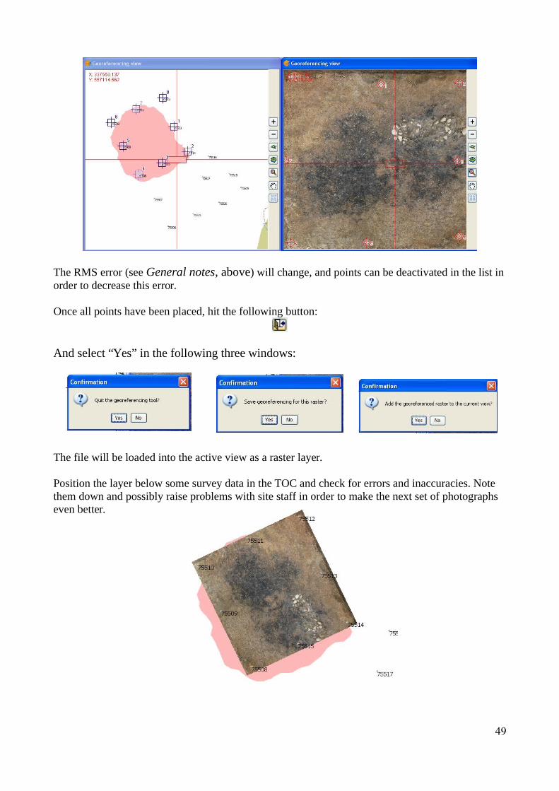
The RMS error (see General notes, above) will change, and points can be deactivated in the list in order to decrease this error.

Once all points have been placed, hit the following button:

And select “Yes” in the following three windows:

The file will be loaded into the active view as a raster layer.

Position the layer below some survey data in the TOC and check for errors and inaccuracies. Note them down and possibly raise problems with site staff in order to make the next set of photographs even better.

49

Problems encountered with gvSIG:

Please see the OA Digital website's section on common gvSIG errors and bugs and troubleshooting:http://oadigital.net/software/gvsigoade/gvsigbugs

50

Appendix 1:Survey Codelist:

This is a codelist designed and produced for basic site survey. The black writing is the code name, the red writing shows the desired format for each point's point_ID. This codelist can be used, and naturally altered for each project's individual survey requirements.

– STN: Station point: OAN1

– BCK: Backsight check: OAN2

– DP P: four per plan – two of these labeled as section points for recognition. Surveyed at ground level for height accuracy – DP70002.1

– DP S: For each Section. Surveyed at ground level for height accuracy – DP70002.1S

– LVLGTOP: Levels taken on top of gridsquares – LVL_765

– LVLGBASE: Levels taken on base of gridsquare – LVL_765

– LVL: general spotheight – LVL1.1, LVL1.2 etc.

– GP: Gridnail – GP1, GP2

– MONO: Monolith: Sample Number

– DEND: Dendrochronological Sample: Sample Number

– CTXTLVL: Level taken on top of a feature. - 70001. Also valid for base of feature – 70001B

– BS: Bulk Sample: Taken at the base of the sample intervention: Sample Number

– WD: Wood-numbers: Taken on top of each piece of wood: Wood Number – 75032

– SF: All finds are recorded by context and have four digits behind the “.”– 70000.0001

– RP: Georectification Point: 75004

– FEP: Archaeological Feature – FEP1.1, FEP1.2 etc.

– DEP: Edge of Deposit – DEP1.1, DEP1.2 etc.

– MOD: Modern feature – Lines. MOD1.1, MOD1.2 etc.

– INT: Intervention through feature, also used for post-ex planning – INT1.1, INT1.2 etc.

– ILOE: Internal limit of excavation – ILOE1.1, ILOE1.2 etc.

– LOE: Limit of excavation – LOE1.1, LOE1.2 etc.

51

Appendix 2:Metadata:

This example can be followed for setting up a logical, easy-to-maintain file-structure and set of GIS data

D:\oa\ project \GIS\Shapefiles\current

Arch_features_old_270709.shpFeatures exported and turned off due to becoming invalid. This is an Archive only. Features may be re-instated from this layer. Not to be mistaken for layer above!!!

Arch_Intervention_230609.shpSurveyed interventions through features – post-ex. Only the edges of the slots are surveyed. INT

Arch_stones_120809.shpExtracted from the Archaeological_features layer – where stones have been surveyed individually.

Archaeological_features_250709.shpCurrent Features layer. Contains all archaeology, except for that archived due to being on a higher level or voided. FEP

Bulk_Samples_290609.shpCurrent total of bulk samples taken. BS

Dendro_samples_050809.shpDendrochronology samples as surveyed. DEND

Deposit_230709.shpEdge of deposits. DEP

DP_P_230709.shpPlan – Drawing Points. Levels on ground surface. DP P

DP_S_260609.shpSection – Drawing Points. Levels on ground surface. DP S

Feature_levels_300609.shpLevels with context numbers taken on top of each feature. CTXTLVL

Haul_Road_polygon.shpHaul Road as surveyed.

ILOE_300609c.shpCurrent Internal Limit of Excavation – dated. “Internal Limit of Excavation” in GIS. ILOE

ILOE_old_300609.shpCropped and old extents of the Internal Limit of Excavation

Levels_General.shp

52

Levels surveyed for other purposes than those listed below. LVL

Modern_features_300609.shpModern features, such as field-drains and trackways. MOD

Monolith_240709.shpMonoliths as surveyed by location – centrepoint MONO

Site_boundary_LOE_100609b.shpExtreme external limit of site - “Limit of Excavation” in GIS. LOE

53

Metadata Matrices – useful examples for data maintenance

a) GIS:

b) Survey:

54

Appendix 3:Drawing of Plans

Use these rules to plan features and to explain the planning of features to others, ensuring that the plans produced by fieldwork staff are all drawn to the same standard of quality!gvSIG requires at least three reference points per plan in order for it to be georeferenced (see p. 45). Georeferencing of plans works best with four points, evenly spaced around the feature and measured accurately on the plan.

55