Surface wave tomography of the western United States …ciei.colorado.edu/ambient_noise/pubs/Lin_etal_2008gji.pdf · Surface wave tomography of the western United States from ambient

February 19, 2008 11:6 Geophysical Journal International gji˙3720

Geophys. J. Int. (2008) doi: 10.1111/j.1365-246X.2008.03720.x

GJI

Sei

smol

ogy

Surface wave tomography of the western United States from ambientseismic noise: Rayleigh and Love wave phase velocity maps

Fan-Chi Lin, Morgan P. Moschetti and Michael H. RitzwollerCenter for Imaging the Earth’s Interior, Department of Physics, University of Colorado at Boulder, Boulder, CO 80309-0390, USA.E-mail: [email protected]

Accepted 2007 December 24. Received 2007 December 22; in original form 2007 May 9

S U M M A R YWe present the results of Rayleigh wave and Love wave phase velocity tomography in thewestern United States using ambient seismic noise observed at over 250 broad-band stationsfrom the EarthScope/USArray Transportable Array and regional networks. All available three-component time-series for the 12-month span between 2005 November 1 and 2006 October31 have been cross-correlated to yield estimated empirical Rayleigh and Love wave Green’sfunctions. The Love wave signals were observed with higher average signal-to-noise ratio(SNR) than Rayleigh wave signals and hence cannot be fully explained by the scattering ofRayleigh waves. Phase velocity dispersion curves for both Rayleigh and Love waves between5 and 40 speriod were measured for each interstation path by applying frequency–time anal-ysis. The average uncertainty and systematic bias of the measurements are estimated using amethod based on analysing thousands of nearly linearly aligned station-triplets. We find thatempirical Green’s functions can be estimated accurately from the negative time derivative ofthe symmetric component ambient noise cross-correlation without explicit knowledge of thesource distribution. The average traveltime uncertainty is less than 1 s at periods shorter than24 s. We present Rayleigh and Love wave phase speed maps at periods of 8, 12, 16,and 20 s.The maps show clear correlations with major geological structures and qualitative agreementwith previous results based on Rayleigh wave group speeds.

Key words: Interferometry; Surface waves and free oscillatons; Seismic tomography; Crustalstructure; North America.

1 I N T RO D U C T I O N

Surface wave tomography using ambient seismic noise, also called

ambient noise tomography (ANT), is becoming an increasingly well-

established method to estimate short period (<20 s) and intermediate

period (between 20 and 50 s) surface wave speeds on both regional

(Sabra et al. 2005; Shapiro et al. 2005; Kang & Shin 2006; Yao

et al. 2006; Lin et al. 2007; Moschetti et al. 2007) and continen-

tal (Bensen et al. 2008; Yang et al. 2007) scales. The applicability

of the method at long periods (>50 s) is also now receiving more

attention (e.g. Bensen et al. 2008; Yang et al. 2007). In these stud-

ies, Rayleigh wave Green’s functions between station-pairs are es-

timated by cross-correlating long time-sequences of ambient noise

recorded simultaneously at both stations. These studies have estab-

lished that, within reasonable tolerances, the measurements are re-

peatable when performed in different seasons, the Green’s functions

agree with earthquake records, dispersion curves agree with those

measured from earthquakes, and the resulting tomography maps co-

here with known geological structures such as sedimentary basins

and mountain ranges. Applied to regional array data, such as the

EarthScope/USArray Transportable Array (TA), PASSCAL exper-

iments, or the Virtual European Broadband Seismic Network, the

resulting dispersion maps display higher resolution and are obtained

to much shorter periods than those typically derived from teleseis-

mic earthquakes. This holds out the prospect to infer considerably

higher resolution information about the crust and uppermost mantle

over extended regions.

To date, these studies have concentrated exclusively on Rayleigh

waves and predominantly have used the estimated empirical Green’s

functions to obtain only measurements of group speed. Yao et al.(2006) was the first to use the empirical Green’s functions to esti-

mate the Rayleigh wave phase speed. The two principle purposes of

this paper are, first, to investigate the extension of ambient noise to-

mography to Love waves and, second, to make phase measurements

in the western United States. In so doing, we use data from the

EarthScope/USArray TA combined with other regional networks in

the western United States. From its inception until 2006 October 31,

over 250 TA stations were deployed in this region and operated for

various lengths of time (Fig. 1). Moschetti et al. (2007) have used

these stations recently to obtain Rayleigh wave group velocity maps

at periods from 8 to 40 s using ANT. We explicitly extend this study

to phase velocity measurements and also show for the first time that

Love wave dispersion also can be measured from ambient noise and

used to produce tomographic maps.

C© 2008 The Authors 1Journal compilation C© 2007 RAS


2 F.-C. Lin, M. P. Moschetti and M. H. Ritzwoller

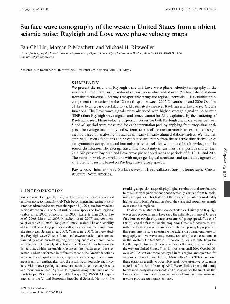
Figure 1. Location of the 253 broad-band stations used in this study, most

from the Transportable Array component of USArray. The colour indicates

the duration of the deployment during this study.

Although coda wave studies (Campillo & Paul 2003; Paul et al.2005) demonstrated that Love wave signals could also be extracted

from the diffusive wavefield, early ambient noise studies focused

on Rayleigh waves at the expense of Love waves because of the

higher locally generated noise on the horizontal components and

general belief that the ambient noise source would be ineffective

at directly generating Love waves. Numerous ambient noise source

studies (e.g. Rhie & Romanowicz 2004, 2006; Stehly et al. 2006;

Yang & Ritzwoller 2008) have concluded that coupling between

ocean waves and the shallow seafloor produces long-range coherent

noise on the vertical component. It has been believed, however, that

it is more difficult to couple ocean waves with horizontal motions

of the seafloor, which would make Love wave generation less effi-

cient than that of Rayleigh waves. We show here that, in fact, Love

waves appear clearly on the transverse–transverse cross-correlations

between most station pairs, at least at periods shorter than 20 s.

The ability to make both Rayleigh and Love wave dispersion

measurements at periods shorter than ∼20 s is important if radial

anisotropy (the bifurcation of Vsv and Vsh) in the crust is to be

observed. Shapiro et al. (2004) inferred strong radial anisotropy in

the Tibetan crust, which they argued is caused by on-going crustal

deformation. This inference is based on observing a discrepancy in

the dispersion characteristics of Rayleigh and Love waves at periods

for which the waves are sensitive to the crust. The thick crust of Tibet

means that surface waves retain sensitivity to crustal structures to

much longer periods than almost everywhere else in the world. For a

crustal Rayleigh-Love discrepancy to be observed across the western

United States, for example, where the average crustal thickness is

less than half that of Tibet, Rayleigh and Love wave dispersion

should be obtained to periods down to at least 10 s. Such periods

are attenuated strongly from distant earthquakes and are largely

unobservable, but are readily observed with ambient noise.

Past work also has concentrated on group rather than phase veloc-

ities for a number of reasons, perhaps most importantly because the

‘initial phase’ of ambient noise cross-correlation was not well under-

stood and has been the subject of some speculation and confusion.

Here we borrow the term ‘initial phase’ used in traditional earth-

quake analysis. Although the ‘initial phase’ here is purely caused

by the inhomogeneity of the noise source distribution, it does share

the same mathematic form and meaning in the context of describing

the estimated Green’s function, as we will show. Theoretical work

done by Lobkis & Weaver (2001), Roux et al. (2005), Sabra et al.(2005) and Snieder (2004b) suggested that phase information in the

surface wave Green’s function can be recovered from the negative

time derivative of the symmetric cross-correlation under the assump-

tion of a spatially homogeneous ambient-noise source distribution.

(The ‘symmetric component cross-correlation’ or ‘symmetric sig-

nal’ is the average of the cross-correlation at positive and negative

correlation lag times.) Under this assumption, Yao et al. (2006) pre-

sented the first phase speed tomography based on ambient noise over

southeast Tibet. However, how this assumption may alter, degrade or

breakdown given the inhomogeneous distribution of ambient noise

sources on earth has been unclear. The inhomogeneous distribution

of noise sources is seen clearly by comparing the positive and neg-

ative lags of the cross-correlations (e.g. Lin et al. 2007). This type

of observation is the basis for recent studies aimed at characterizing

ambient noise sources (e.g. Stehly et al. 2006; Yang & Ritzwoller

2008). Yao et al. (2006) have also suggested that an inhomogeneous

source distribution may account for part of the 1–3 per cent incon-

sistency they observed between phase velocity measurements made

by the ambient noise method and the traditional earthquake-based

two-station method between periods of 20–30 s.

Phase velocity measurements are desirable for the following rea-

sons. First, as we show, the uncertainty of the phase velocity mea-

surement is much smaller than that of the group velocity measure-

ment. Second, within the same period band, phase velocity has a

deeper sensitivity kernel and, therefore, constrains deeper velocity

structures. Third, the dispersion relation for group velocity can be

calculated from the dispersion relation for phase velocity, but the

converse is not true.

In this paper, we address whether robust phase velocity measure-

ments can be obtained from ambient noise without explicit knowl-

edge of the source distribution. We use an empirical three-station

method, discussed in Section 4.2, to test this hypothesis and also to

identify systematic errors and the average uncertainty of real phase

velocity measurements. Several previous studies have used the sea-

sonal variability of the measurement to estimate their uncertainty

(e.g. Bensen et al. 2007; Lin et al. 2007; Yang et al. 2007). Our

method, however, avoids the possibility of repeated false measure-

ments and systematic error. Synthetic cross-correlations based on

different source distributions, discussed in Section 6.2, suggest that

the ‘initial phase’ of the estimated Green’s function would be ap-

proximately zero if the source distribution were to vary smoothly

C© 2008 The Authors, GJI

Journal compilation C© 2007 RAS


Rayleigh and Love wave phase velocity maps 3

over the constructive interference region. Combined with the re-

sult of the three-station method, we show that even though ambi-

ent noise sources have an inhomogeneous azimuthal distribution,

ambient noise is distributed sufficiently homogeneously so that no

additional phase shift is required in the estimated Green’s function

to account for irregularities in the source distribution.

We emphasize here that the only difference between ambient noise

seismology and earthquake based seismology is the method used to

obtain the waveforms used in the analysis. We extensively use terms

borrowed from traditional earthquake seismology, such as ‘initial

phase’, ‘far field approximation’ and ‘signal-to-noise ratio’ (SNR),

to analyse and describe the estimated Green’s function obtained by

the cross-correlation of the ambient noise because these terms have

the same meaning in this context.

The outline of this paper is as follows. We describe the method to

obtain the estimated Green’s functions for both Rayleigh and Love

waves in Section 2. Evidence for the existence and retrievability

of Love waves is presented in Section 3. In Section 4, we describe

the method used to obtain the phase velocity measurements and the

three-station method is developed to estimate the systematic errors

and the average uncertainty of the measurements. Tomography maps

at periods of 8, 12, 16 and 20 s for both Rayleigh and Love wave

phase speeds are presented in Section 5. Throughout the paper, the

straight ray theory is used and we focus on phase velocity measure-

ments between periods of 8 and 24 s, where the highest SNRs are

observed, on average.

2 DATA P RO C E S S I N G T O P RO D U C E

T H E E S T I M AT E D G R E E N ’ S

F U N C T I O N S

We analysed continuous data from over 250 broad-band stations in

the western United States (Fig. 1) recorded between 2005 November

1 and 2006 October 31. Data from all three components (east, north,

vertical) were used, and cross-correlations between all possible pairs

of components from the two-stations were computed. The method

to obtain the estimated Green’s function is similar to that described

for Rayleigh waves by Bensen et al. (2007). We summarize it briefly

here with a concentration on the Love wave data processing.

All data are processed on a daily basis and then are stacked (su-

perposed and added together) later. The mean, trend, and instrument

response of the daily component (E, N, Z) seismograms are first re-

moved and bandpass filtered between periods of 5 and 100 s. To

speed up the process, we do not rotate the components into the

radial (R) and transverse (T) directions for each station-pair until

the component cross-correlations (E–E, E–N, N–N, N–E) are per-

formed. Earthquake signals and instrumental irregularities are then

removed by temporal normalization (Bensen et al. 2007). In order

to postpone the component rotation until after cross-correlation, the

east and north components are temporally normalized together. To

achieve this, both components are first bandpass filtered between

15 and 50 s, a band that contains the most energetic surface wave

signals from earthquakes. For each time point, the mean of the ab-

solute value of each seismogram is computed in the 128 s window

centred on that point. The values of the east and north components

are compared, and the larger is used to define the inverse weight for

that time point. That weight is then applied to both the north and east

component time-series bandpassed between 5 and 100 s. This pro-

cess effectively suppresses earthquake signals and is commutative

with the rotation operator.

After temporal normalization, the signals are whitened in fre-

quency. Before whitening, ambient noise is most energetic in the

microseismic band below 20-s period. Frequency whitening is car-

ried out to broaden the period band of the dispersion measurement.

Again, to maintain the commutativity of the rotation operator, the

east and north signals are whitened together. To do this, we first

smooth the east amplitude spectrum by taking the average of the

amplitude of spectrum with a 0.01 Hz moving window in the fre-

quency domain. Because the spectra of both components are similar

in shape, on average, we whiten both of them together simply by

weighting the east and north signals in the frequency domain by

the inverse of this smoothed east spectrum. In general, the phase

dispersion measurement is not sensitive to the spectrum variation

but to the phase variation. Hence, this simple whitening process

does improve the spectral content and at the same time allows us to

postpone the rotation step. Other methods, such as weighting by the

mean of the two spectra or their product, produce similar results.

This concludes the data preparation prior to cross-correlation.

north–north, north–east, east–east and east–north cross-

correlations are calculated between every station-pair for each day-

length record. We stack all available daily cross-correlations for

each station-pair into one time-series to enhance the SNR. Be-

cause all operators are commutative with the rotation operator, the

transverse–transverse, transverse–radial, radial–radial and radial–

transverse cross-correlations between each station-pair can be cal-

culated by a linear combination of those four components with co-

efficients related to the interstation azimuth θ and backazimuth ψ

angles. These angles are defined by setting the first station as the

‘event’ location and the second station as the receiver location so

that the rotation is:⎛⎜⎜⎝T TR RT RRT

⎞⎟⎟⎠ =

⎛⎜⎜⎝− cos θ cos ψ cos θ sin ψ − sin θ sin ψ sin θ cos ψ

− sin θ sin ψ − sin θ cos ψ − cos θ cos ψ − cos θ sin ψ

− cos θ sin ψ − cos θ cos ψ sin θ cos ψ sin θ sin ψ

− sin θ cos ψ sin θ sin ψ cos θ sin ψ − cos θ cos ψ

⎞⎟⎟⎠

×

⎛⎜⎜⎝E EE NN NN E

⎞⎟⎟⎠ . (1)

Note that both the radial components and the transverse com-

ponents at both stations point to the same direction, respectively,

under our notation, as shown in Fig. 2. The choice to rotate the

north and east components into the transverse and radial compo-

nents after cross-correlation makes the computation considerably

more efficient and space saving. We have compared the results from

both cases and no differences are observed.

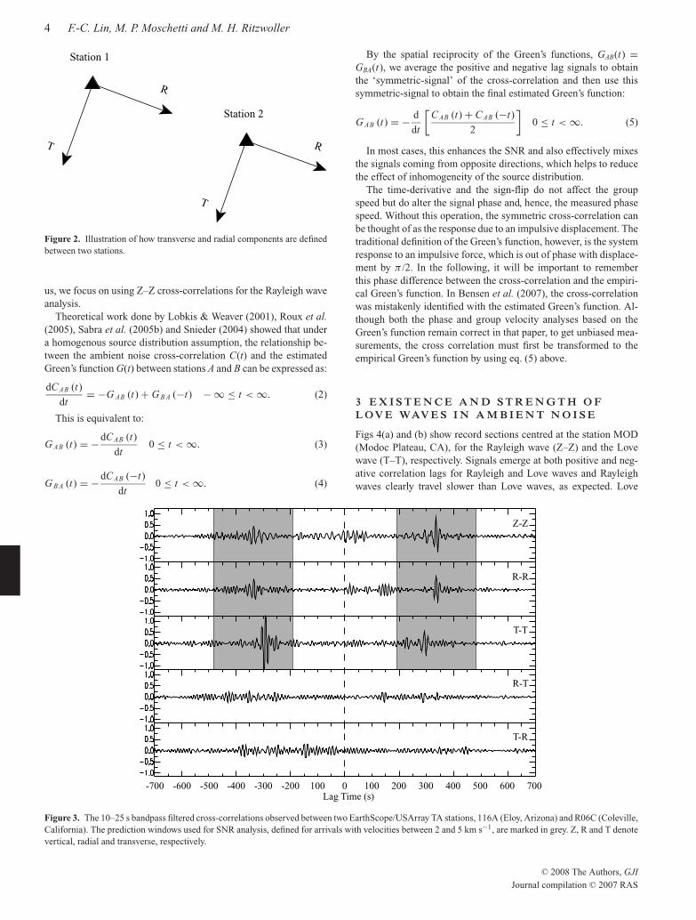
An example of the resulting cross-correlation between stations

116A and R06C is shown in Fig. 3. Both signals at positive and nega-

tive correlation lag times, respectively, are observed, corresponding

to waves propagating in opposite directions between the stations.

A clear difference in arrival time is observed between the wave-

forms on the transverse–transverse (T–T) and radial–radial (R–R)

cross-correlations. Signal arrival times on the vertical–vertical (Z–

Z) cross-correlation and the R–R cross-correlation are similar, and

result from the Rayleigh wave. The T–T cross-correlation exhibits

the faster Love wave arrival. Although both the Z–Z and R–R cross-

correlations contain the same Rayleigh wave signal, the Z–Z cross-

correlation generally has a higher SNR. Hence, like others before





Station 1

R

T

Station 2

R

T

Figure 2. Illustration of how transverse and radial components are defined

between two stations.

us, we focus on using Z–Z cross-correlations for the Rayleigh wave

analysis.

Theoretical work done by Lobkis & Weaver (2001), Roux et al.(2005), Sabra et al. (2005b) and Snieder (2004) showed that under

a homogenous source distribution assumption, the relationship be-

tween the ambient noise cross-correlation C(t) and the estimated

Green’s function G(t) between stations A and B can be expressed as:

dCAB (t)

dt= −G AB (t) + G B A (−t) − ∞ ≤ t < ∞. (2)

This is equivalent to:

G AB (t) = −dCAB (t)

dt0 ≤ t < ∞. (3)

G B A (t) = −dCAB (−t)

dt0 ≤ t < ∞. (4)

By the spatial reciprocity of the Green’s functions, GAB(t) =GBA(t), we average the positive and negative lag signals to obtain

the ‘symmetric-signal’ of the cross-correlation and then use this

symmetric-signal to obtain the final estimated Green’s function:

G AB (t) = − d

dt

[CAB (t) + CAB (−t)

2

]0 ≤ t < ∞. (5)

In most cases, this enhances the SNR and also effectively mixes

the signals coming from opposite directions, which helps to reduce

the effect of inhomogeneity of the source distribution.

The time-derivative and the sign-flip do not affect the group

speed but do alter the signal phase and, hence, the measured phase

speed. Without this operation, the symmetric cross-correlation can

be thought of as the response due to an impulsive displacement. The

traditional definition of the Green’s function, however, is the system

response to an impulsive force, which is out of phase with displace-

ment by π /2. In the following, it will be important to remember

this phase difference between the cross-correlation and the empiri-

cal Green’s function. In Bensen et al. (2007), the cross-correlation

was mistakenly identified with the estimated Green’s function. Al-

though both the phase and group velocity analyses based on the

Green’s function remain correct in that paper, to get unbiased mea-

surements, the cross correlation must first be transformed to the

empirical Green’s function by using eq. (5) above.

3 E X I S T E N C E A N D S T R E N G T H O F

L OV E WAV E S I N A M B I E N T N O I S E

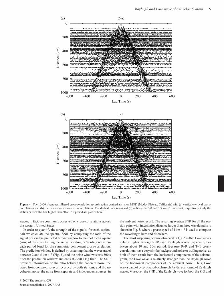
Figs 4(a) and (b) show record sections centred at the station MOD

(Modoc Plateau, CA), for the Rayleigh wave (Z–Z) and the Love

wave (T–T), respectively. Signals emerge at both positive and neg-

ative correlation lags for Rayleigh and Love waves and Rayleigh

waves clearly travel slower than Love waves, as expected. Love

Lag Time (s)

Z-Z

R-R

T-T

R-T

T-R

0 100 200 300 400 500 600 700-700 -600 -500 -400 -300 -200 100

Figure 3. The 10–25 s bandpass filtered cross-correlations observed between two EarthScope/USArray TA stations, 116A (Eloy, Arizona) and R06C (Coleville,

California). The prediction windows used for SNR analysis, defined for arrivals with velocities between 2 and 5 km s−1, are marked in grey. Z, R and T denote

vertical, radial and transverse, respectively.





Lag Time (s)

Dis

tan

ce (

km

)

0 600400200-200-400-600

0

1000

800

600

400

200

Lag Time (s)

Dis

tan

ce (

km

)

0 600400200-200-400-600

0

1000

800

600

400

200

T-T

Z-Z(a)

(b)

Figure 4. The 10–50 s bandpass filtered cross-correlation record section centred at station MOD (Modoc Plateau, California) with (a) vertical–vertical cross-

correlations and (b) transverse–transverse cross-correlations. The dashed lines in (a) and (b) indicate the 3.0 and 3.3 km s−1 moveout, respectively. Only the

station pairs with SNR higher than 20 at 18 s period are plotted here.

waves, in fact, are commonly observed on cross-correlations across

the western United States.

In order to quantify the strength of the signals, for each station-

pair we calculate the spectral SNR by computing the ratio of the

signal peak in the predicted arrival window to the root mean square

(rms) of the noise trailing the arrival window, or ‘trailing noise’, in

each period band for the symmetric component cross-correlation.

The prediction window is defined by assuming that the waves travel

between 2 and 5 km s−1 (Fig. 3), and the noise window starts 500 s

after the prediction window and ends at 2700 s lag time. The SNR

provides information on the ratio between the coherent noise, the

noise from common sources recorded by both stations, and the in-

coherent noise, the noise from separate and independent sources, in

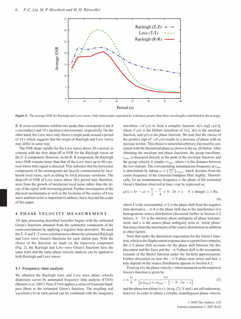
the ambient noise record. The resulting average SNR for all the sta-

tion pairs with interstation distance larger than three wavelengths is

shown in Fig. 5, where a phase speed of 4 km s−1 is used to compute

the wavelength here and elsewhere.

The most surprising feature observed in Fig. 5 is that Love waves

exhibit higher average SNR than Rayleigh waves, especially be-

tween about 10 and 20-s period. Because R–R and T–T cross-

correlations have very similar background noise or trailing noise, as

both of them result from the horizontal components of the seismo-

gram, the Love wave is relatively stronger than the Rayleigh wave

on the horizontal components of the ambient noise. Thus, Love

waves cannot be generated exclusively by the scattering of Rayleigh

waves. Moreover, the SNR of the Rayleigh wave for both the Z–Z and





0

5

10

15

20

25

30

35

5 10 15 20 25 30 35 40

Rayleigh (Z-Z)

Love (T-T)

Rayleigh (R-R)

Period (s)

Aver

age

SN

R

Figure 5. The average SNR for Rayleigh and Love waves. Only station pairs separated by a distance greater than three wavelengths contributed to the average.

R–R cross-correlations exhibits two peaks that correspond to the 8

s (secondary) and 16 s (primary) microseisms, respectively. On the

other hand, the Love wave only shows a single peak around a period

of 14 s which suggests that the origin of Rayleigh and Love waves

may differ in some way.

The SNR drops rapidly for the Love waves above 20-s period, in

contrast with the slow drop-off in SNR for the Rayleigh waves on

the Z–Z component. However, on the R–R component, the Rayleigh

wave SNR remains lower than that of the Love wave up to 40-s pe-

riod where little signal is detected. This indicates that the horizontal

components of the seismograms are heavily contaminated by inco-

herent local noise, such as tilting by local pressure variations. The

drop-off of SNR of Love waves above 20-s period may, therefore,

arise from the growth of incoherent local noise rather than the de-

cay of the signal with increasing period. Further investigation of the

physical mechanisms as well as the locations of the source of Love

wave ambient noise is important to address, but is beyond the scope

of this paper.

4 P H A S E V E L O C I T Y M E A S U R E M E N T

All data processing described hereafter begins with the estimated

Green’s functions obtained from the symmetric component of the

cross-correlations by applying a negative time-derivative. We used

the Z–Z and T–T cross-correlations to obtain the estimated Rayleigh

and Love wave Green’s functions for each station pair. With the

choice of the direction we made on the transverse component

(Fig. 2), the Rayleigh and Love wave Green’s functions have the

same form and the same phase velocity analysis can be applied to

both Rayleigh and Love waves.

4.1 Frequency–time analysis

We obtained the Rayleigh wave and Love wave phase velocity

dispersion curves by automated frequency–time analysis (FTAN)

(Bensen et al. 2007). First, FTAN applies a series of Gaussian band-

pass filters to the estimated Green’s function. The resulting real

waveform f (t) at each period can be combined with the imaginary

waveform +iFH (t) to form a complex function A(t) exp[ iϕ(t)],where FH (t) is the Hilbert transform of f (t), A(t) is the envelope

function, and ϕ(t) is the phase function. We note that the choice of

the positive sign of +iFH (t) results in a decrease of phase with an

increase in time. This choice is somewhat arbitrary; but must be con-

sistent with the theoretical phase as shown in the eq. (6) below. After

obtaining the envelope and phase functions, the group traveltime,

tmax, is measured directly as the peak of the envelope function, and

the group velocity is simply r/tmax, where r is the distance between

the two stations. The corresponding instantaneous frequency at tmax

is determined by taking ω = [ ∂ϕ(t)∂t ]t=tmax , which deviates from the

centre frequency of the Gaussian bandpass filter slightly. Theoreti-

cally, for an instantaneous frequency ω the phase of the estimated

Green’s function observed at time t can be expressed as:

ϕ(t) = kr − ωt + π

2− π

4+ N · 2π + λ N ∈ Integer, λ ∈ Re,

(6)

where k is the wavenumber, π /2 is the phase shift from the negative

time-derivative, −π /4 is the phase shift due to the interference of a

homogeneous source distribution (discussed further in Section 6.2

below), N · 2π is the intrinsic phase ambiguity of phase measure-

ment, and λ is the source phase ambiguity term or ‘initial phase’

that arises from the uncertainty of the source distribution in addition

to other factors.

Note that under the theoretical expectation for the Green’s func-

tion, which is the displacement response due to a point force impulse,

the π /2 phase shift accounts for the phase shift between the dis-

placement and the force and the −π /4 phase shift is the asymptotic

remnant of the Bessel function under the far-field approximation.

Further discussion on how the −π /4 phase term arises and how λ

may depend on the source distribution appears in Section 6.2.

From eq. (6), the phase velocity c when measured on the empirical

Green’s function is given by

c = ω

k= rω[

ϕ (tmax) + ωtmax − π

4− N · 2π − λ

] (7)

and the phase traveltime is r/c. In eq. (7), N and λ are still unknowns,

however. In order to obtain a reliable, unambiguous phase velocity





2.5

3

3.5

4

4.5

5

5 10 15 20 25 30 35 40Period (s)

Vel

oci

ty (

km

/s)

(a)

(b)

2.5

3

3.5

4

4.5

5

5 10 15 20 25 30 35 40Period (s)

Vel

oci

ty (

km

/s)

Rayleigh Love

1st Reference curve

N off by 1

Correct N

1st Reference curve

Revised

2nd Reference curve

Preliminary

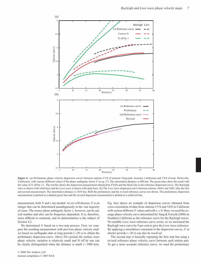
Figure 6. (a) Preliminary phase velocity dispersion curves between stations CVS (Carmenet Vineyards, Sonoma, California) and VES (Vestal, Porterville,

California), with various different values of the phase ambiguity factor N in eq. (7). The interstation distance is 409 km. The green lines show the result with

the value of N off by ±1. The red line shows the dispersion measurement obtained by FTAN and the black line is the reference dispersion curve. The Rayleigh

wave is shown with solid lines and the Love wave is shown with dash lines. (b) The Love wave dispersion curve between stations A04A and 109C after the first

and second measurement. The interstation distance is 1819 km. Both the preliminary and the revised reference curves are shown. The preliminary dispersion

measurement is plotted as a dashed green line and the revised dispersion measurement is plotted as a solid red line.

measurement, both N and λ are needed. As we will discuss, N is an

integer that can be determined unambiguously in the vast majority

of cases. The source phase ambiguity factor λ, however, can be any

real number and also can be frequency dependent. It is, therefore,

more difficult to constrain, and its determination is the subject of

Section 4.2.

We determined N based on a two-step process. First, we com-

pare the resulting measurement with previous phase velocity stud-

ies based on earthquake data at long periods (>20 s) to obtain the

preliminary dispersion curve. Above 20-s period, the surface wave

phase velocity variation is relatively small and N off by one can

be clearly distinguished when the distance is small (<1000 km).

Fig. 6(a) shows an example of dispersion curves obtained from

cross-correlation of data from stations CVS and VES in California

with various different N values and with λ = 0. Here, we used the av-

erage phase velocity curve determined by Yang & Forsyth (2006) in

Southern California as the reference curve for the Rayleigh waves.

No suitable Love wave reference curve exists, so we increased the

Rayleigh wave curve by 9 per cent to give the Love wave reference.

By applying a smoothness constraint to the dispersion curves, N at

shorter periods (<20 s) can also be resolved.

The second step is basically repeating the first step but using a

revised reference phase velocity curve between each station pair.

To get a more accurate reference curve, we used the preliminary





dispersion measurements obtained using the method described

above combined with the selection criteria described in Section 5 to

invert for preliminary phase speed maps for periods between 6 and

28 s. We used these maps to estimate the dispersion curves for every

station pair which we then used as the reference curves to redeter-

mine N . This second step effectively resolves the 2π ambiguity that

cannot be resolved in the first step either due to the lack of good

signal at long periods or when the station-pair is at a long distance.

Perhaps more importantly, this step makes dispersion measurement

a self-consistent process and less dependent on a priori assump-

tions. More Love wave measurements, but fewer than 4 per cent,

were changed after the second step than Rayleigh wave, probably

due to the degradation of SNR at long periods. Fig. 6(b) shows an

example of Love wave measurement between stations A04A (Legoe

Bay, WA) and 109C (Camp Elliot, CA). Due to the extremely long

distance (>1800 km) and the lack of good measurement above 20 s,

the preliminary measurement had N off by one, but is corrected

after the second step. Although this two-steps process effectively

allows for identification of the appropriate N for most cases, the

same method does not work for λ.

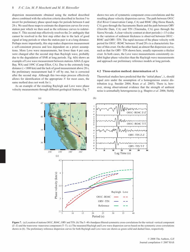
As an example of the resulting Rayleigh and Love wave phase

velocity measurements through different geological features, Fig. 7

shows two sets of symmetric component cross-correlations and the

resulting phase velocity dispersion curves. The path between O01C

(Eel River Conservation Camp, CA) and R04C (Big Horse Ranch,

CA) goes through the Sacramento Basin and the path between ORV

(Oroville Dam, CA) and TIN (Tinemaha, CA) goes through the

Sierra Nevada. A clear velocity contrast at short periods (<15 s) due

to the variation of sediment thickness is observed between O01C–

R04C and ORV–TIN. The rapid increase of the phase velocity with

period for O01C–RO4C between 10 and 20 s is a characteristic fea-

ture of thin crust. On the other hand, an almost flat dispersion curve,

such as that for ORV–TIN shown here, usually represents a thicker

crust. In both cases, the Love wave measurements consistently ex-

hibit higher phase velocities than the Rayleigh wave measurements

and approach our preliminary reference models at long periods.

4.2 Three-station method: determination of λ

Theoretical studies have predicted that the ‘initial phase’, λ, should

equal zero under the assumption of a homogeneous source dis-

tribution (e.g. Sneider 2004; Roux et al. 2005). There is, how-

ever, strong observational evidence that the strength of ambient

noise is azimuthally heterogeneous (e.g. Shapiro et al. 2006; Stehly

2.5

3

3.5

4

4.5

5 10 15 20 25 30 35 40

236˚ 238˚ 240˚ 242˚

36˚

38˚

40˚

42˚

O01CR04C

ORV

TIN

O01C–RO4C Z-Z

O01C–RO4C T-T

ORV–TIN Z-Z

ORV–TIN T-T

Reference

ORV–TIN

Rayleigh Love

Lag Time (s)

O01C–RO4C

(a) (b)

(c)

Period (s)

Phas

e vel

oci

ty (

km

/s)

Figure 7. (a) Location of stations O01C, R04C, ORV and TIN. (b) The 5–40 s bandpass filtered symmetric cross-correlations for the vertical–vertical component

(Z–Z) and the transverse–transverse component (T–T). (c) The measured Rayleigh and Love wave dispersion curves based on the symmetric cross-correlations

shown in (b). The preliminary reference dispersion curves for both Rayleigh and Love wave are shown as green solid and dashed lines, respectively.





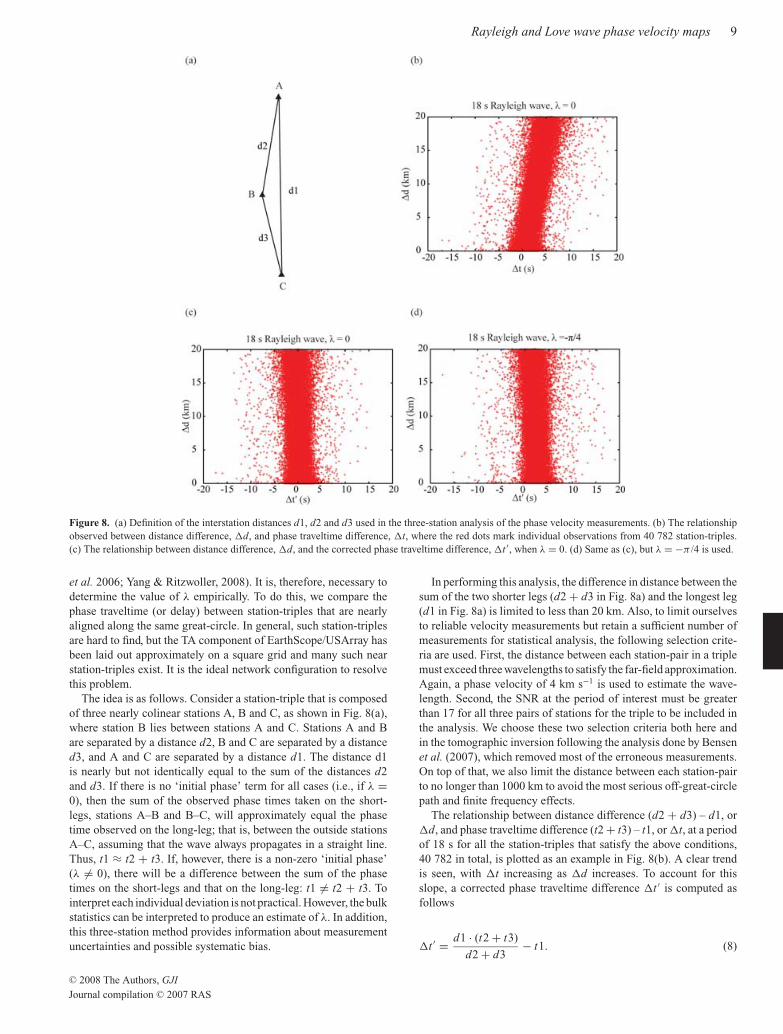
Figure 8. (a) Definition of the interstation distances d1, d2 and d3 used in the three-station analysis of the phase velocity measurements. (b) The relationship

observed between distance difference, d, and phase traveltime difference, t, where the red dots mark individual observations from 40 782 station-triples.

(c) The relationship between distance difference, d, and the corrected phase traveltime difference, t ′, when λ = 0. (d) Same as (c), but λ = −π /4 is used.

et al. 2006; Yang & Ritzwoller, 2008). It is, therefore, necessary to

determine the value of λ empirically. To do this, we compare the

phase traveltime (or delay) between station-triples that are nearly

aligned along the same great-circle. In general, such station-triples

are hard to find, but the TA component of EarthScope/USArray has

been laid out approximately on a square grid and many such near

station-triples exist. It is the ideal network configuration to resolve

this problem.

The idea is as follows. Consider a station-triple that is composed

of three nearly colinear stations A, B and C, as shown in Fig. 8(a),

where station B lies between stations A and C. Stations A and B

are separated by a distance d2, B and C are separated by a distance

d3, and A and C are separated by a distance d1. The distance d1

is nearly but not identically equal to the sum of the distances d2

and d3. If there is no ‘initial phase’ term for all cases (i.e., if λ =0), then the sum of the observed phase times taken on the short-

legs, stations A–B and B–C, will approximately equal the phase

time observed on the long-leg; that is, between the outside stations

A–C, assuming that the wave always propagates in a straight line.

Thus, t1 ≈ t2 + t3. If, however, there is a non-zero ‘initial phase’

(λ = 0), there will be a difference between the sum of the phase

times on the short-legs and that on the long-leg: t1 = t2 + t3. To

interpret each individual deviation is not practical. However, the bulk

statistics can be interpreted to produce an estimate of λ. In addition,

this three-station method provides information about measurement

uncertainties and possible systematic bias.

In performing this analysis, the difference in distance between the

sum of the two shorter legs (d2 + d3 in Fig. 8a) and the longest leg

(d1 in Fig. 8a) is limited to less than 20 km. Also, to limit ourselves

to reliable velocity measurements but retain a sufficient number of

measurements for statistical analysis, the following selection crite-

ria are used. First, the distance between each station-pair in a triple

must exceed three wavelengths to satisfy the far-field approximation.

Again, a phase velocity of 4 km s−1 is used to estimate the wave-

length. Second, the SNR at the period of interest must be greater

than 17 for all three pairs of stations for the triple to be included in

the analysis. We choose these two selection criteria both here and

in the tomographic inversion following the analysis done by Bensen

et al. (2007), which removed most of the erroneous measurements.

On top of that, we also limit the distance between each station-pair

to no longer than 1000 km to avoid the most serious off-great-circle

path and finite frequency effects.

The relationship between distance difference (d2 + d3) – d1, or

d, and phase traveltime difference (t2 + t3) – t1, or t, at a period

of 18 s for all the station-triples that satisfy the above conditions,

40 782 in total, is plotted as an example in Fig. 8(b). A clear trend

is seen, with t increasing as d increases. To account for this

slope, a corrected phase traveltime difference t ′ is computed as

follows

t ′ = d1 · (t2 + t3)

d2 + d3− t1. (8)





Δt’ (s)

Num

ber

of

Mea

sure

men

ts

Rayleigh wave, λ = 0

12 s

18 s

24 s

Δt’ (s)

Num

ber

of

Mea

sure

men

ts

Rayleigh wave, λ =-π/4

Δt’ (s)

Num

ber

of

Mea

sure

men

ts

Love wave, λ = -π/4

12 s

18 s

Δt’ (s)

Num

ber

of

Mea

sure

men

ts

Love wave, λ = 0

12 s

18 s

(a) (b)

(c) (d)

0

2000

4000

6000

8000

10000

12000

-10 -5 0 5 10

0

2000

4000

6000

8000

10000

12000

-10 -5 0 5 10

12 s

18 s

24 s

0

2000

4000

6000

8000

10000

12000

-10 -5 0 5 10

0

2000

4000

6000

8000

10000

12000

-10 -5 0 5 10

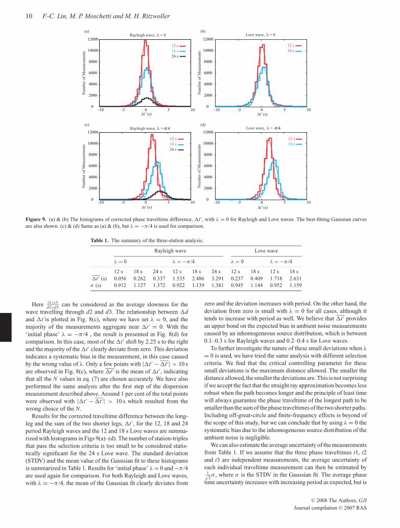
Figure 9. (a) & (b) The histograms of corrected phase traveltime difference, t ′, with λ = 0 for Rayleigh and Love waves. The best-fitting Gaussian curves

are also shown. (c) & (d) Same as (a) & (b), but λ = −π /4 is used for comparison.

Table 1. The summary of the three-station analysis.

Rayleigh wave Love wave

λ = 0 λ = −π /4 λ = 0 λ = −π /4

12 s 18 s 24 s 12 s 18 s 24 s 12 s 18 s 12 s 18 s

t ′ (s) 0.056 0.262 0.337 1.535 2.486 3.291 0.237 0.409 1.718 2.631

σ (s) 0.912 1.127 1.372 0.922 1.139 1.381 0.945 1.144 0.952 1.159

Here t2+t3d2+d3

can be considered as the average slowness for the

wave travelling through d2 and d3. The relationship between dand t ′is plotted in Fig. 8(c), where we have set λ = 0, and the

majority of the measurements aggregate near t ′ = 0. With the

‘initial phase’ λ = −π /4 , the result is presented in Fig. 8(d) for

comparison. In this case, most of the t ′ shift by 2.25 s to the right

and the majority of the t ′ clearly deviate from zero. This deviation

indicates a systematic bias in the measurement, in this case caused

by the wrong value of λ. Only a few points with |t ′ − t ′| > 10 s

are observed in Fig. 8(c), where t ′ is the mean of t ′, indicating

that all the N values in eq. (7) are chosen accurately. We have also

performed the same analysis after the first step of the dispersion

measurement described above. Around 1 per cent of the total points

were observed with |t ′ − t ′| > 10 s which resulted from the

wrong choice of the N .

Results for the corrected traveltime difference between the long-

leg and the sum of the two shorter legs, t ′, for the 12, 18 and 24

period Rayleigh waves and the 12 and 18 s Love waves are summa-

rized with histograms in Figs 9(a)–(d). The number of station-triples

that pass the selection criteria is too small to be considered statis-

tically significant for the 24 s Love wave. The standard deviation

(STDV) and the mean value of the Gaussian fit to these histograms

is summarized in Table 1. Results for ‘initial phase’ λ = 0 and −π /4

are used again for comparison. For both Rayleigh and Love waves,

with λ = −π /4, the mean of the Gaussian fit clearly deviates from

zero and the deviation increases with period. On the other hand, the

deviation from zero is small with λ = 0 for all cases, although it

tends to increase with period as well. We believe that t ′ provides

an upper bond on the expected bias in ambient noise measurements

caused by an inhomogeneous source distribution, which is between

0.1–0.3 s for Rayleigh waves and 0.2–0.4 s for Love waves.

To further investigate the nature of these small deviations when λ

= 0 is used, we have tried the same analysis with different selection

criteria. We find that the critical controlling parameter for these

small deviations is the maximum distance allowed. The smaller the

distance allowed, the smaller the deviations are. This is not surprising

if we accept the fact that the straight ray approximation becomes less

robust when the path becomes longer and the principle of least time

will always guarantee the phase traveltime of the longest path to be

smaller than the sum of the phase traveltimes of the two shorter paths.

Including off-great-circle and finite-frequency effects is beyond of

the scope of this study, but we can conclude that by using λ = 0 the

systematic bias due to the inhomogeneous source distribution of the

ambient noise is negligible.

We can also estimate the average uncertainty of the measurements

from Table 1. If we assume that the three phase traveltimes t1, t2and t3 are independent measurements, the average uncertainty of

each individual traveltime measurement can then be estimated by1√3σ , where σ is the STDV in the Gaussian fit. The average phase

time uncertainty increases with increasing period as expected, but is





less than 1 s for all cases. An uncertainty of less than half a second

would be difficult to attain because 1 sample per second time-series

are used in this study. This estimation of the phase traveltime un-

certainty is independent of the repeatability of the measurements

at different times, which has been performed in other studies (e.g.

Bensen et al. 2007; Yang et al. 2007), and provides a new way to

estimate the average traveltime uncertainty. This uncertainty, how-

ever, is characteristic of the interstation spacings used in this study,

and would be expected to grow with increasing interstation distance.

The three-station method developed here confirms that λ = 0 is

a good approximation for the majority of the measurements and

bias caused by an inhomogeneous source distribution is minimal.

The results also provide insight into the quality of the phase ve-

locity measurements. Overall, the phase traveltime measurements

in this study display a negligible systematic error and an average

uncertainty of less than 1 s for periods shorter than 24 s. The impli-

cation of these results for the distribution of ambient noise sources

is discussed in Section 6.2.

5 P H A S E V E L O C I T Y T O M O G R A P H Y

F O R R AY L E I G H A N D L OV E WAV E S

The selection of the most reliable measurements for tomography is

based on three criteria. First, the distance between two stations must

be longer than three wavelengths to satisfy the far-field approxima-

tion. Again, 4 km s−1 is used as a rule-of-thumb to estimate the

wavelength. This introduces an effective long-period cut-off of r/12

(in seconds) between stations separated by distance r in km. For ex-

ample, stations separated by 120 km will not return measurements

at periods greater than 10 s. Second, the SNR must be higher than

17 at the period of interest. These two criteria are chosen following

Bensen et al. (2007). Third, each measurement must be coherent

with other measurements as measured by its ability to be fit by a

smooth tomographic map.

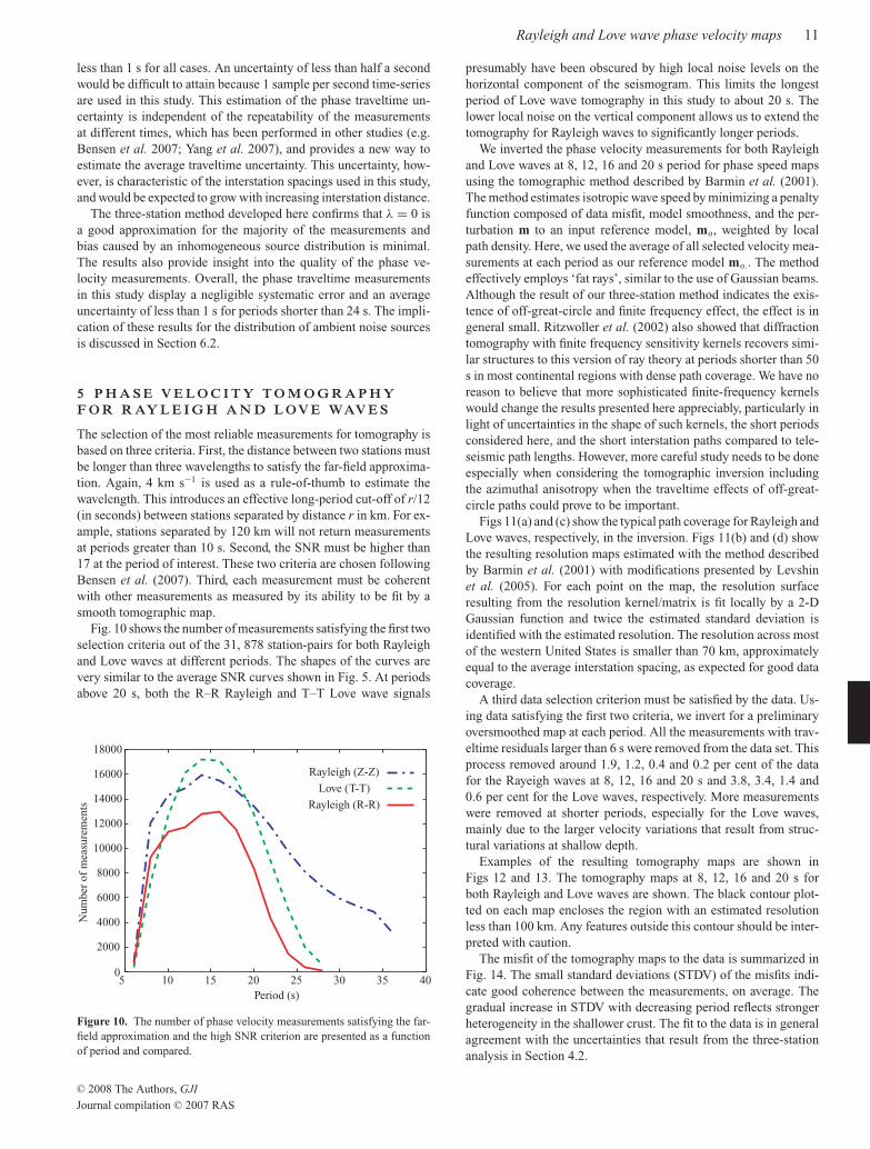
Fig. 10 shows the number of measurements satisfying the first two

selection criteria out of the 31, 878 station-pairs for both Rayleigh

and Love waves at different periods. The shapes of the curves are

very similar to the average SNR curves shown in Fig. 5. At periods

above 20 s, both the R–R Rayleigh and T–T Love wave signals

Rayleigh (Z-Z)

Love (T-T)

Rayleigh (R-R)

Period (s)

Nu

mb

er o

f m

easu

rem

ents

0

2000

4000

6000

8000

10000

12000

14000

16000

18000

5 10 15 20 25 30 35 40

Figure 10. The number of phase velocity measurements satisfying the far-

field approximation and the high SNR criterion are presented as a function

of period and compared.

presumably have been obscured by high local noise levels on the

horizontal component of the seismogram. This limits the longest

period of Love wave tomography in this study to about 20 s. The

lower local noise on the vertical component allows us to extend the

tomography for Rayleigh waves to significantly longer periods.

We inverted the phase velocity measurements for both Rayleigh

and Love waves at 8, 12, 16 and 20 s period for phase speed maps

using the tomographic method described by Barmin et al. (2001).

The method estimates isotropic wave speed by minimizing a penalty

function composed of data misfit, model smoothness, and the per-

turbation m to an input reference model, mo, weighted by local

path density. Here, we used the average of all selected velocity mea-

surements at each period as our reference model mo.. The method

effectively employs ‘fat rays’, similar to the use of Gaussian beams.

Although the result of our three-station method indicates the exis-

tence of off-great-circle and finite frequency effect, the effect is in

general small. Ritzwoller et al. (2002) also showed that diffraction

tomography with finite frequency sensitivity kernels recovers simi-

lar structures to this version of ray theory at periods shorter than 50

s in most continental regions with dense path coverage. We have no

reason to believe that more sophisticated finite-frequency kernels

would change the results presented here appreciably, particularly in

light of uncertainties in the shape of such kernels, the short periods

considered here, and the short interstation paths compared to tele-

seismic path lengths. However, more careful study needs to be done

especially when considering the tomographic inversion including

the azimuthal anisotropy when the traveltime effects of off-great-

circle paths could prove to be important.

Figs 11(a) and (c) show the typical path coverage for Rayleigh and

Love waves, respectively, in the inversion. Figs 11(b) and (d) show

the resulting resolution maps estimated with the method described

by Barmin et al. (2001) with modifications presented by Levshin

et al. (2005). For each point on the map, the resolution surface

resulting from the resolution kernel/matrix is fit locally by a 2-D

Gaussian function and twice the estimated standard deviation is

identified with the estimated resolution. The resolution across most

of the western United States is smaller than 70 km, approximately

equal to the average interstation spacing, as expected for good data

coverage.

A third data selection criterion must be satisfied by the data. Us-

ing data satisfying the first two criteria, we invert for a preliminary

oversmoothed map at each period. All the measurements with trav-

eltime residuals larger than 6 s were removed from the data set. This

process removed around 1.9, 1.2, 0.4 and 0.2 per cent of the data

for the Rayeigh waves at 8, 12, 16 and 20 s and 3.8, 3.4, 1.4 and

0.6 per cent for the Love waves, respectively. More measurements

were removed at shorter periods, especially for the Love waves,

mainly due to the larger velocity variations that result from struc-

tural variations at shallow depth.

Examples of the resulting tomography maps are shown in

Figs 12 and 13. The tomography maps at 8, 12, 16 and 20 s for

both Rayleigh and Love waves are shown. The black contour plot-

ted on each map encloses the region with an estimated resolution

less than 100 km. Any features outside this contour should be inter-

preted with caution.

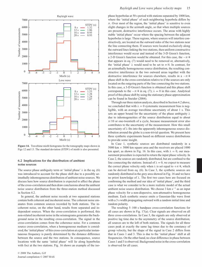
The misfit of the tomography maps to the data is summarized in

Fig. 14. The small standard deviations (STDV) of the misfits indi-

cate good coherence between the measurements, on average. The

gradual increase in STDV with decreasing period reflects stronger

heterogeneity in the shallower crust. The fit to the data is in general

agreement with the uncertainties that result from the three-station

analysis in Section 4.2.





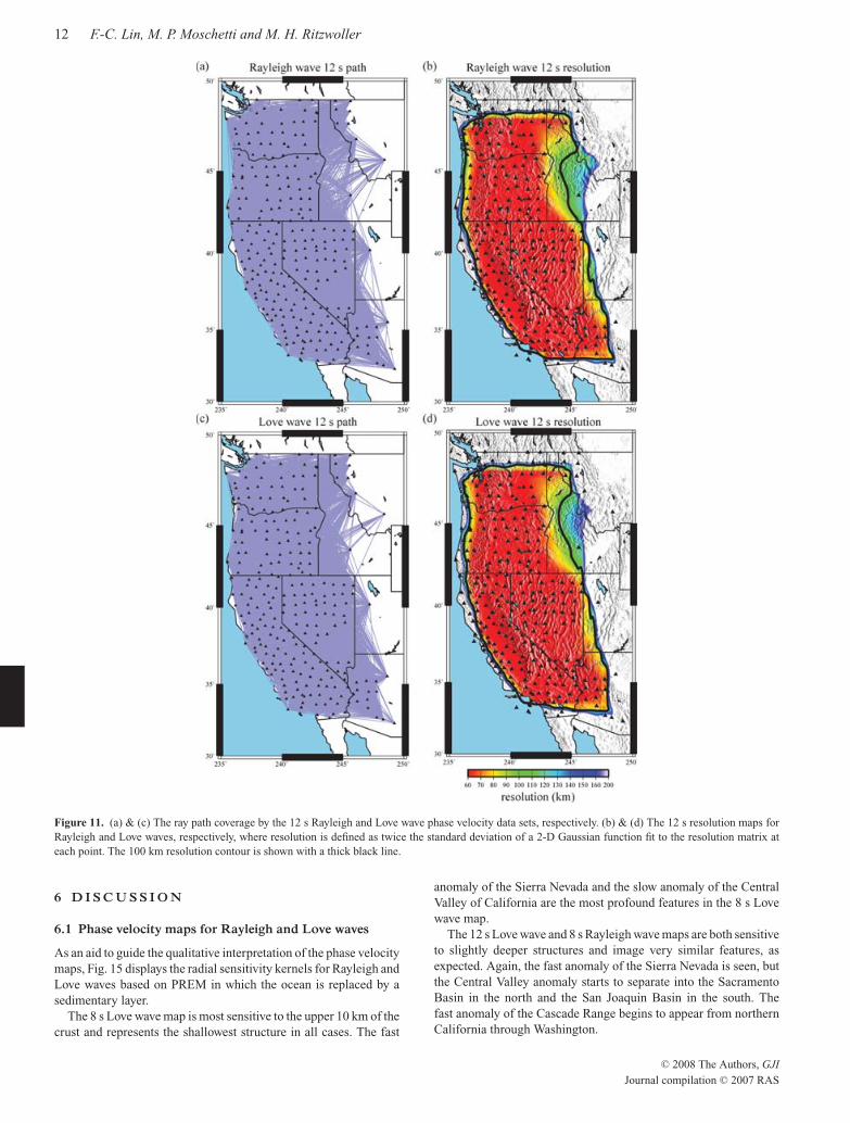
Figure 11. (a) & (c) The ray path coverage by the 12 s Rayleigh and Love wave phase velocity data sets, respectively. (b) & (d) The 12 s resolution maps for

Rayleigh and Love waves, respectively, where resolution is defined as twice the standard deviation of a 2-D Gaussian function fit to the resolution matrix at

each point. The 100 km resolution contour is shown with a thick black line.

6 D I S C U S S I O N

6.1 Phase velocity maps for Rayleigh and Love waves

As an aid to guide the qualitative interpretation of the phase velocity

maps, Fig. 15 displays the radial sensitivity kernels for Rayleigh and

Love waves based on PREM in which the ocean is replaced by a

sedimentary layer.

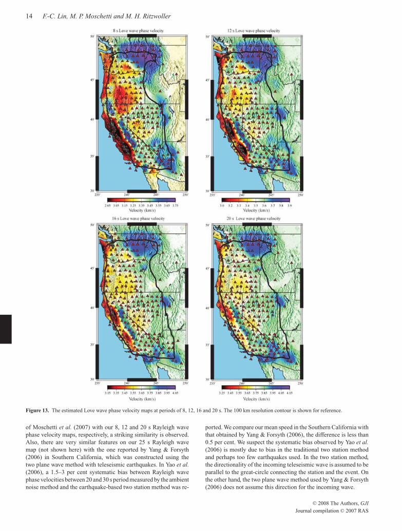
The 8 s Love wave map is most sensitive to the upper 10 km of the

crust and represents the shallowest structure in all cases. The fast

anomaly of the Sierra Nevada and the slow anomaly of the Central

Valley of California are the most profound features in the 8 s Love

wave map.

The 12 s Love wave and 8 s Rayleigh wave maps are both sensitive

to slightly deeper structures and image very similar features, as

expected. Again, the fast anomaly of the Sierra Nevada is seen, but

the Central Valley anomaly starts to separate into the Sacramento

Basin in the north and the San Joaquin Basin in the south. The

fast anomaly of the Cascade Range begins to appear from northern

California through Washington.





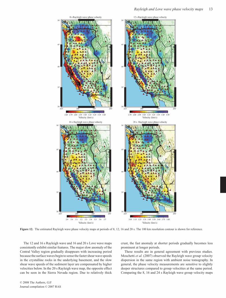
Figure 12. The estimated Rayleigh wave phase velocity maps at periods of 8, 12, 16 and 20 s. The 100 km resolution contour is shown for reference.

The 12 and 16 s Rayleigh wave and 16 and 20 s Love wave maps

consistently exhibit similar features. The major slow anomaly of the

Central Valley region gradually disappears with increasing period

because the surface waves begin to sense the faster shear wave speeds

in the crystalline rocks in the underlying basement, and the slow

shear wave speeds of the sediment layer are compensated by higher

velocities below. In the 20 s Rayleigh wave map, the opposite effect

can be seen in the Sierra Nevada region. Due to relatively thick

crust, the fast anomaly at shorter periods gradually becomes less

prominent at longer periods.

These results are in general agreement with previous studies.

Moschetti et al. (2007) observed the Rayleigh wave group velocity

dispersion in the same region with ambient noise tomography. In

general, the phase velocity measurements are sensitive to slightly

deeper structures compared to group velocities at the same period.

Comparing the 8, 16 and 24 s Rayleigh wave group velocity maps





Figure 13. The estimated Love wave phase velocity maps at periods of 8, 12, 16 and 20 s. The 100 km resolution contour is shown for reference.

of Moschetti et al. (2007) with our 8, 12 and 20 s Rayleigh wave

phase velocity maps, respectively, a striking similarity is observed.

Also, there are very similar features on our 25 s Rayleigh wave

map (not shown here) with the one reported by Yang & Forsyth

(2006) in Southern California, which was constructed using the

two plane wave method with teleseismic earthquakes. In Yao et al.(2006), a 1.5–3 per cent systematic bias between Rayleigh wave

phase velocities between 20 and 30 s period measured by the ambient

noise method and the earthquake-based two station method was re-

ported. We compare our mean speed in the Southern California with

that obtained by Yang & Forsyth (2006), the difference is less than

0.5 per cent. We suspect the systematic bias observed by Yao et al.(2006) is mostly due to bias in the traditional two station method

and perhaps too few earthquakes used. In the two station method,

the directionality of the incoming teleseismic wave is assumed to be

parallel to the great-circle connecting the station and the event. On

the other hand, the two plane wave method used by Yang & Forsyth

(2006) does not assume this direction for the incoming wave.





0

1000

2000

3000

4000

5000

6000

7000

-5 0 5

0

1000

2000

3000

4000

5000

6000

7000

Misfit (s)

Misfit (s)

Num

ber

of

mea

sure

men

tsN

um

ber

of

mea

sure

men

tsRayleigh wave

Love wave

8 s12 s16 s20 s

STDV (s)1.321.060.950.93

8 s12 s16 s20 s

STDV (s)1.531.281.241.07

1 2 3 4-1-4 -3 -2

-5 0 51 2 3 4-1-4 -3 -2

Figure 14. Traveltime misfit histograms for the tomography maps shown in

Figs 12 and 13. The standard deviation (STDV) of misfit is also presented.

6.2 Implications for the distribution of ambient

noise sources

The source phase ambiguity term or ‘initial phase’ λ in the eq. (6)

was introduced to account for the phase shift due to a possibly az-

imuthally inhomogeneous distribution of ambient noise sources. We

discuss here how source distribution is expected to affect the phase

of the cross-correlation and then draw conclusions about the ambient

noise source distribution from the three-station method discussed

in Section 4.2.

In general, the ambient noise records at two separated stations

contain both coherent and incoherent noise. The coherent noise em-

anates from common sources recorded by both stations. The in-

coherent noise, on the other hand, results from separated and in-

dependent sources. When the cross-correlation is performed, this

non-related incoherent noise in the seismograms generates the back-

ground noise in the resulting cross-correlation. The signal in the

cross-correlation comes from the coherence noise. For a common

source cross-correlation, when a homogeneous medium is consid-

ered, the ‘initial phase’ of this cross-correlation at a particular instan-

taneous frequency is purely determined by the distance difference

between the source and the two stations. In consequence, source

locations with the same ‘initial phase’ will lie along hyperbolas

with foci at the two stations. Fig. 16 shows an example of the iso-

phase hyperbolas at 50 s period with stations separated by 1000 km,

where the ‘initial phase’ of each neighboring hyperbola differs by

π . Over most of the region, the ‘initial phase’ is sensitive to even

slight changes in the azimuth angle, so that when multiple sources

are present, destructive interference occurs. The areas with highly

stable ‘initial phase’ occur where the spacing between the adjacent

hyperbolas is large. These regions, where sources will interfere con-

structively, are located on the outward sides of the two stations near

the line connecting them. If sources were located exclusively along

the outward lines linking the two stations, then uniform constructive

interference would occur and instead of the 3-D Green’s function,

a 2-D Green’s function would be obtained. For this case, the −π /4

that appears in eq. (7) would need to be removed or, alternatively,

the ‘initial phase’ λ would need to be set to π /4. In contrast, for

an azimuthally homogeneous source distribution, the resulting con-

structive interference in the two outward areas together with the

destructive interference for sources elsewhere, results in a −π /4

phase shift in the cross-correlation relative to if the sources are only

located on the outgoing parts of the line connecting the two stations.

In this case, a 3-D Green’s function is obtained and this phase shift

corresponds to the −π /4 in eq. (7); λ = 0 in this case. Analytical

proof of this phase shift by using the stationary phase approximation

can be found in Sneider (2004).

Through our three station analysis, described in Section 4.2 above,

we concluded that with λ = 0 systematic measurement bias is neg-

ligible, with an average traveltime uncertainty of about 1 s. This

sets an upper bound for the uncertainty of the phase ambiguity λ

due to inhomogeneities of the source distribution equal to about

π /10 or one-twentieth of a cycle, because measurement error also

contributes to the uncertainty of the measurement. How this small

uncertainty of λ fits into the apparently inhomogeneous source dis-

tribution around the globe is a non-trivial question. We present here

three synthetic experiments based on different source distributions

to provide some insight.

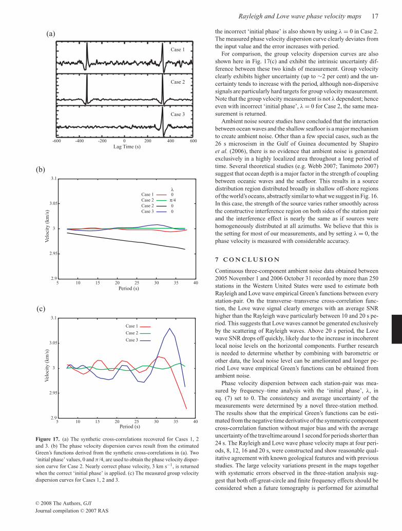
In Case 1, synthetic sources are distributed randomly in a

5000 km × 5000 km square area and the receivers are placed 1000

km apart, as shown in Fig. 16. In this case, with λ = 0, our mea-

surement procedure is expected to return the input phase velocity. In

Case 2, the sources are randomly distributed, but are confined to the

line connecting the stations. Instead of λ = 0, we expect to measure

the correct phase velocity only when λ is set equal to +π /4, which

can be derived from eq. (6). In Case 3, the synthetic sources are

randomly distributed in the grey area showed in Fig. 16 and we have

no priori knowledge of λ. The first two cases here are focused on

confirming the method and our idea of ‘initial phase’, and the third

case is what we consider to be a more realistic model of the actual

ambient noise source distribution. We choose 3 km s−1 as an input

phase velocity for a non-dispersive, non-attenuative homogeneous

medium. Each synthetic source emits a Gaussian-like wave front

with a 3 s width propagating outward with a random initial time and

random polarity.

The resulting 5–100 s bandpass cross-correlation functions for

all cases are shown in Fig. 17(a). Clear signals are observed on all

three cross-correlations. In Case 3, the signals are only observed at

positive lag time due to the asymmetry of the source distribution;

all sources are to the left of both stations. The signals for all three

cases peak at exactly the same lag times due to the constancy of

group velocity, but the shape of the signal in Case 2 differs from

that in Cases 1 and 3. This is due to the ‘initial phase’ shift at all

frequencies. On the other hand, no clear difference in phase between

Cases 1 and 3 is observed. Background noise in the cross-correlation

is observed for all cases.





0 0.01 0.02 0.03 0.04 0.05 0.06 0.07 0.08 0.09

0

20

40

60

80

8 s12 s16 s20 s

0 0.01 0.02 0.03 0.04 0.05 0.06 0.07 0.08 0.09

0

20

40

60

80 0.1

8 s12 s16 s20 s

Rayleigh wave Love wave

Normalized sensitivity

Dep

th (

km

)

Normalized sensitivity

Dep

th (

km

)

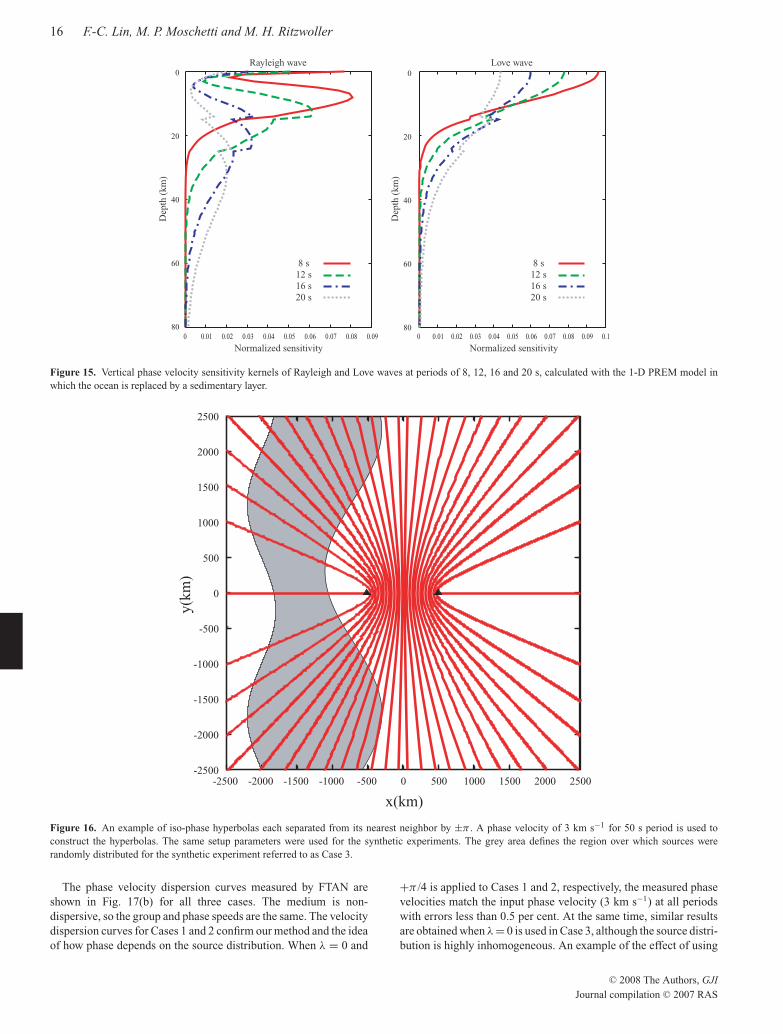
Figure 15. Vertical phase velocity sensitivity kernels of Rayleigh and Love waves at periods of 8, 12, 16 and 20 s, calculated with the 1-D PREM model in

which the ocean is replaced by a sedimentary layer.

-2500

-2000

-1500

-1000

-500

0

500

1000

1500

2000

2500

-2500 -2000 -1500 -1000 -500 0 500 1000 1500 2000 2500

x(km)

y(k

m)

Figure 16. An example of iso-phase hyperbolas each separated from its nearest neighbor by ±π . A phase velocity of 3 km s−1 for 50 s period is used to

construct the hyperbolas. The same setup parameters were used for the synthetic experiments. The grey area defines the region over which sources were

randomly distributed for the synthetic experiment referred to as Case 3.

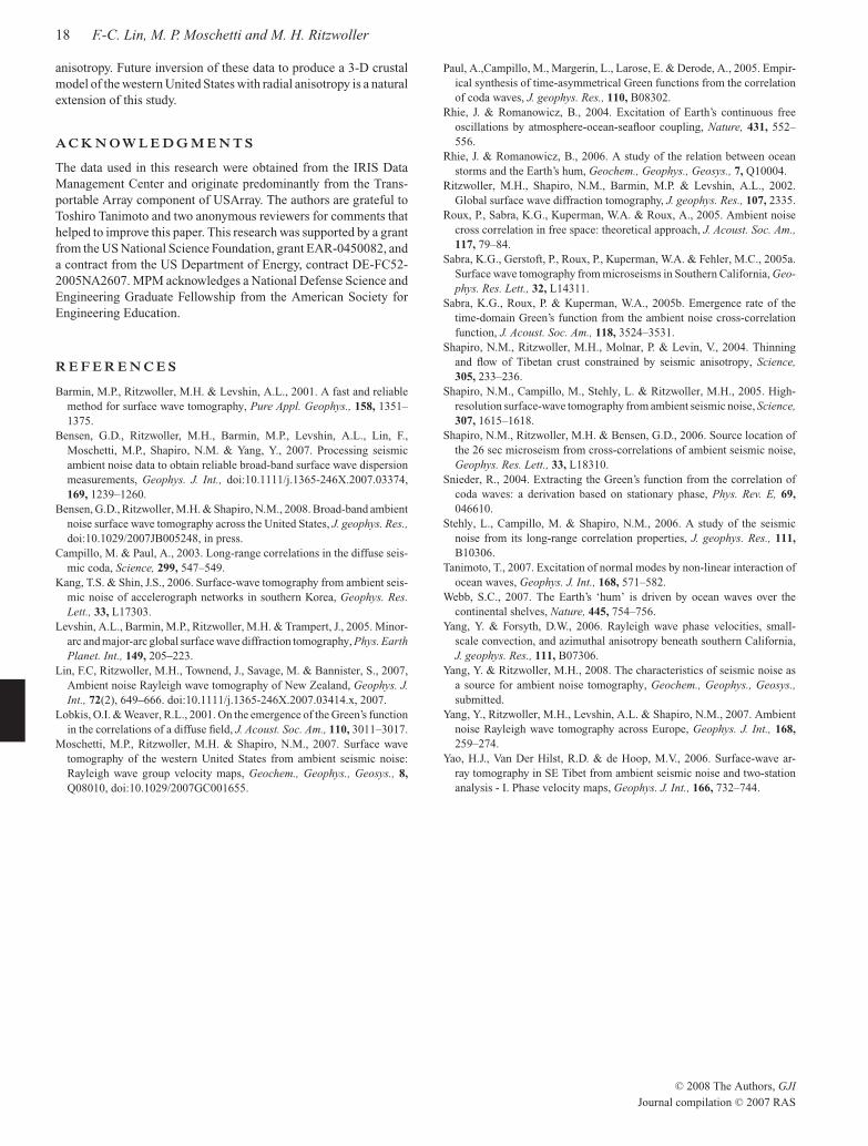
The phase velocity dispersion curves measured by FTAN are

shown in Fig. 17(b) for all three cases. The medium is non-

dispersive, so the group and phase speeds are the same. The velocity

dispersion curves for Cases 1 and 2 confirm our method and the idea

of how phase depends on the source distribution. When λ = 0 and

+π /4 is applied to Cases 1 and 2, respectively, the measured phase

velocities match the input phase velocity (3 km s−1) at all periods

with errors less than 0.5 per cent. At the same time, similar results

are obtained when λ = 0 is used in Case 3, although the source distri-

bution is highly inhomogeneous. An example of the effect of using





2.9

2.95

3

3.05

3.1

5 10 15 20 25 30 35 40

Case 1

Case 3

Case 2

0

0

0

Case 2 π/4

0 200 400 600-200-400-600

Lag Time (s)

Case 1

Case 2

Case 3

Period (s)

Vel

oci

ty (

km

/s)

2.9

2.95

3

3.05

3.1

5 10 15 20 25 30 35 40Period (s)

Vel

oci

ty (

km

/s)

(a)

(b)

(c)

Case 1

Case 3

Case 2

λ

Figure 17. (a) The synthetic cross-correlations recovered for Cases 1, 2

and 3. (b) The phase velocity dispersion curves result from the estimated

Green’s functions derived from the synthetic cross-correlations in (a). Two

‘initial phase’ values, 0 and π /4, are used to obtain the phase velocity disper-

sion curve for Case 2. Nearly correct phase velocity, 3 km s−1, is returned

when the correct ‘initial phase’ is applied. (c) The measured group velocity

dispersion curves for Cases 1, 2 and 3.

the incorrect ‘initial phase’ is also shown by using λ = 0 in Case 2.

The measured phase velocity dispersion curve clearly deviates from

the input value and the error increases with period.

For comparison, the group velocity dispersion curves are also

shown here in Fig. 17(c) and exhibit the intrinsic uncertainty dif-

ference between these two kinds of measurement. Group velocity

clearly exhibits higher uncertainty (up to ∼2 per cent) and the un-

certainty tends to increase with the period, although non-dispersive

signals are particularly hard targets for group velocity measurement.

Note that the group velocity measurement is not λ dependent; hence

even with incorrect ‘initial phase’, λ = 0 for Case 2, the same mea-

surement is returned.

Ambient noise source studies have concluded that the interaction

between ocean waves and the shallow seafloor is a major mechanism

to create ambient noise. Other than a few special cases, such as the

26 s microseism in the Gulf of Guinea documented by Shapiro

et al. (2006), there is no evidence that ambient noise is generated

exclusively in a highly localized area throughout a long period of

time. Several theoretical studies (e.g. Webb 2007; Tanimoto 2007)

suggest that ocean depth is a major factor in the strength of coupling

between oceanic waves and the seafloor. This results in a source

distribution region distributed broadly in shallow off-shore regions

of the world’s oceans, abstractly similar to what we suggest in Fig. 16.

In this case, the strength of the source varies rather smoothly across

the constructive interference region on both sides of the station pair

and the interference effect is nearly the same as if sources were

homogeneously distributed at all azimuths. We believe that this is

the setting for most of our measurements, and by setting λ = 0, the

phase velocity is measured with considerable accuracy.

7 C O N C L U S I O N

Continuous three-component ambient noise data obtained between

2005 November 1 and 2006 October 31 recorded by more than 250

stations in the Western United States were used to estimate both

Rayleigh and Love wave empirical Green’s functions between every

station-pair. On the transverse–transverse cross-correlation func-

tion, the Love wave signal clearly emerges with an average SNR

higher than the Rayleigh wave particularly between 10 and 20 s pe-

riod. This suggests that Love waves cannot be generated exclusively

by the scattering of Rayleigh waves. Above 20 s period, the Love

wave SNR drops off quickly, likely due to the increase in incoherent

local noise levels on the horizontal components. Further research

is needed to determine whether by combining with barometric or

other data, the local noise level can be ameliorated and longer pe-

riod Love wave empirical Green’s functions can be obtained from

ambient noise.

Phase velocity dispersion between each station-pair was mea-

sured by frequency–time analysis with the ‘initial phase’, λ, in

eq. (7) set to 0. The consistency and average uncertainty of the

measurements were determined by a novel three-station method.

The results show that the empirical Green’s functions can be esti-

mated from the negative time derivative of the symmetric component

cross-correlation function without major bias and with the average

uncertainty of the traveltime around 1 second for periods shorter than

24 s. The Rayleigh and Love wave phase velocity maps at four peri-

ods, 8, 12, 16 and 20 s, were constructed and show reasonable qual-

itative agreement with known geological features and with previous

studies. The large velocity variations present in the maps together

with systematic errors observed in the three-station analysis sug-

gest that both off-great-circle and finite frequency effects should be

considered when a future tomography is performed for azimuthal





anisotropy. Future inversion of these data to produce a 3-D crustal

model of the western United States with radial anisotropy is a natural

extension of this study.

A C K N O W L E D G M E N T S

The data used in this research were obtained from the IRIS Data

Management Center and originate predominantly from the Trans-

portable Array component of USArray. The authors are grateful to

Toshiro Tanimoto and two anonymous reviewers for comments that

helped to improve this paper. This research was supported by a grant

from the US National Science Foundation, grant EAR-0450082, and

a contract from the US Department of Energy, contract DE-FC52-

2005NA2607. MPM acknowledges a National Defense Science and

Engineering Graduate Fellowship from the American Society for

Engineering Education.

R E F E R E N C E S

Barmin, M.P., Ritzwoller, M.H. & Levshin, A.L., 2001. A fast and reliable

method for surface wave tomography, Pure Appl. Geophys., 158, 1351–

1375.

Bensen, G.D., Ritzwoller, M.H., Barmin, M.P., Levshin, A.L., Lin, F.,

Moschetti, M.P., Shapiro, N.M. & Yang, Y., 2007. Processing seismic

ambient noise data to obtain reliable broad-band surface wave dispersion

measurements, Geophys. J. Int., doi:10.1111/j.1365-246X.2007.03374,

169, 1239–1260.

Bensen, G.D., Ritzwoller, M.H. & Shapiro, N.M., 2008. Broad-band ambient

noise surface wave tomography across the United States, J. geophys. Res.,doi:10.1029/2007JB005248, in press.

Campillo, M. & Paul, A., 2003. Long-range correlations in the diffuse seis-

mic coda, Science, 299, 547–549.

Kang, T.S. & Shin, J.S., 2006. Surface-wave tomography from ambient seis-

mic noise of accelerograph networks in southern Korea, Geophys. Res.Lett., 33, L17303.

Levshin, A.L., Barmin, M.P., Ritzwoller, M.H. & Trampert, J., 2005. Minor-

arc and major-arc global surface wave diffraction tomography, Phys. EarthPlanet. Int., 149, 205–223.

Lin, F.C, Ritzwoller, M.H., Townend, J., Savage, M. & Bannister, S., 2007,

Ambient noise Rayleigh wave tomography of New Zealand, Geophys. J.Int., 72(2), 649–666. doi:10.1111/j.1365-246X.2007.03414.x, 2007.

Lobkis, O.I. & Weaver, R.L., 2001. On the emergence of the Green’s function

in the correlations of a diffuse field, J. Acoust. Soc. Am., 110, 3011–3017.

Moschetti, M.P., Ritzwoller, M.H. & Shapiro, N.M., 2007. Surface wave

tomography of the western United States from ambient seismic noise:

Rayleigh wave group velocity maps, Geochem., Geophys., Geosys., 8,Q08010, doi:10.1029/2007GC001655.

Paul, A.,Campillo, M., Margerin, L., Larose, E. & Derode, A., 2005. Empir-

ical synthesis of time-asymmetrical Green functions from the correlation

of coda waves, J. geophys. Res., 110, B08302.

Rhie, J. & Romanowicz, B., 2004. Excitation of Earth’s continuous free

oscillations by atmosphere-ocean-seafloor coupling, Nature, 431, 552–

556.

Rhie, J. & Romanowicz, B., 2006. A study of the relation between ocean

storms and the Earth’s hum, Geochem., Geophys., Geosys., 7, Q10004.

Ritzwoller, M.H., Shapiro, N.M., Barmin, M.P. & Levshin, A.L., 2002.

Global surface wave diffraction tomography, J. geophys. Res., 107, 2335.

Roux, P., Sabra, K.G., Kuperman, W.A. & Roux, A., 2005. Ambient noise

cross correlation in free space: theoretical approach, J. Acoust. Soc. Am.,117, 79–84.

Sabra, K.G., Gerstoft, P., Roux, P., Kuperman, W.A. & Fehler, M.C., 2005a.

Surface wave tomography from microseisms in Southern California, Geo-phys. Res. Lett., 32, L14311.

Sabra, K.G., Roux, P. & Kuperman, W.A., 2005b. Emergence rate of the

time-domain Green’s function from the ambient noise cross-correlation

function, J. Acoust. Soc. Am., 118, 3524–3531.

Shapiro, N.M., Ritzwoller, M.H., Molnar, P. & Levin, V., 2004. Thinning

and flow of Tibetan crust constrained by seismic anisotropy, Science,305, 233–236.

Shapiro, N.M., Campillo, M., Stehly, L. & Ritzwoller, M.H., 2005. High-

resolution surface-wave tomography from ambient seismic noise, Science,307, 1615–1618.

Shapiro, N.M., Ritzwoller, M.H. & Bensen, G.D., 2006. Source location of

the 26 sec microseism from cross-correlations of ambient seismic noise,

Geophys. Res. Lett., 33, L18310.

Snieder, R., 2004. Extracting the Green’s function from the correlation of

coda waves: a derivation based on stationary phase, Phys. Rev. E, 69,046610.

Stehly, L., Campillo, M. & Shapiro, N.M., 2006. A study of the seismic

noise from its long-range correlation properties, J. geophys. Res., 111,B10306.

Tanimoto, T., 2007. Excitation of normal modes by non-linear interaction of

ocean waves, Geophys. J. Int., 168, 571–582.

Webb, S.C., 2007. The Earth’s ‘hum’ is driven by ocean waves over the

continental shelves, Nature, 445, 754–756.

Yang, Y. & Forsyth, D.W., 2006. Rayleigh wave phase velocities, small-

scale convection, and azimuthal anisotropy beneath southern California,

J. geophys. Res., 111, B07306.

Yang, Y. & Ritzwoller, M.H., 2008. The characteristics of seismic noise as

a source for ambient noise tomography, Geochem., Geophys., Geosys.,submitted.

Yang, Y., Ritzwoller, M.H., Levshin, A.L. & Shapiro, N.M., 2007. Ambient

noise Rayleigh wave tomography across Europe, Geophys. J. Int., 168,259–274.

Yao, H.J., Van Der Hilst, R.D. & de Hoop, M.V., 2006. Surface-wave ar-

ray tomography in SE Tibet from ambient seismic noise and two-station

analysis - I. Phase velocity maps, Geophys. J. Int., 166, 732–744.



Documents

Surface wave tomography of the western United States …ciei.colorado.edu/ambient_noise/pubs/Lin_etal_2008gji.pdf · Surface wave tomography of the western United States from ambient