Surface Vortices and Pressures in Suction Intakes of ...kdm.p.lodz.pl/articles/2012/6_B_P.pdf · Mechanics and Mechanical Engineering Vol. 16, No. 1 (2012) 51{71 ⃝c Technical University

$Page 1: Surface Vortices and Pressures in Suction Intakes of ...kdm.p.lodz.pl/articles/2012/6_B_P.pdf · Mechanics and Mechanical Engineering Vol. 16, No. 1 (2012) 51{71 ⃝c Technical University$
Mechanics and Mechanical Engineering

Vol. 16, No. 1 (2012) 51–71c⃝ Technical University of Lodz

Surface Vortices and Pressures in SuctionIntakes of Vertical Axial–Flow Pumps

Andrzej B laszczykAdam PapierskiRadosaw KunickiMariusz Susik

Institute of TurbomachineryTechnical University of [email protected]@[email protected]

Received (13 October 2012)

Revised (15 December 2012)

Accepted (5 January 2013)

In the article, there are introduced results of numerical computations of unsteady flowin the intake of large vertical pumps verified by results of the measurements made onthe test stand.

Comparative analysis ofresults ofnumerical computations,pressuremeasurements andthe observation of surface vortices, have confirmed the justness of a chosen computationalmethod.

Keywords: Pump, inlet channel, cooling water system.

1. Introduction

Due to the increased demand for electrical and thermal power there are new powerunits being built in Poland, as well as currently working being modernized.

New huge power units and these being upgradedin terms of theincreased power,both require large supplies of the cooling water to the turbine condenser.

Most often there are mixed flow or axial flow pumps in the vertical system builtinto cooling water systems.

Due to the vertical construction of cooling water pumps, in their intake area,the flowing in water must change its’ direction from horizontal to vertical. Changeof the flow direction of huge amounts of water, inintake channels, is the existencecause of hydraulic phenomena which could disrupt or even stop the work of pumps.Changing theflow directionfrom horizontal toverticalis implementedin formed suc-tion intakes, into whichthe water is drawn from wet wells.

52 B laszczyk, A., Papierski, A., Kunicki, R., Susik, M.

The flow and hydraulic phenomena which take place in open wet wells play amajor role in supplyinga liquidto thepumpimpeller.

Suction intake and outlet are final elements of the water intake system in pumps.

Scheme of theanalyzed real facility with marked elements of the pump intakesystem andits chosen geometrical parameters of the facility shown in the Fig. 1

The real pumping station facility (Fig. 1) consists of: the screen chamber (1),where are trash screens (2) used to roughlypurifythe water supply flowing in fromthehigh–water source, (3) the rotary screen which task is to thorough purify thewater from apollution, (4) the open wet well, (5) theformed suction intake and (6)the place for the cooling water pump installation.

In case of the wrong design of the formed suction intake and the open wet well,the flow can be characterized with typical of the unsteady flow:

• subsurface vortices (formed suction intake),

• surface vortices (open wet well),

• non–uniform distribution ofthe absolutevelocity axialcomponent in the im-peller eye (suction chamber),

• liquid vortices in front of the impeller eye (suction chamber).

2. The open wet well

Wet well along with the built–in rotary screen covers an areacontainedbetween theoutlet ofthe wet welland theformed suction intake. Wet well is an essential elementof inflow channels supplying liquid to the axial flow pumps or mixed flow with thevertical axis, because of the water level, flow and geometry have the influence on theliquid inflowcharacterto the formed suction intake by controlling over thestructureofthe flowin theinlet areaof a pump (Fig. 1).

Figure 1 The real facility – system of the open wet well

Surface Vortices and Pressures in Suction ... 53

The integral element of the wet well is a construction of the rotary screen, whichalso has an essential impact on the occurring inside hydraulic phenomena.

Vorticesarisingat the wet wellsurface, subsurfaceandbottomcan moveto the areaofthe pump inlet, causing anon–uniformflow ofthe liquidto theimpeller.

A particularthreat tothe pumparesurfacevortices, which can cause anaeration ofthepumpand, consequently, adrop of the efficiency to zeroanddamagetothe machine.

Surface vortex is a phenomena arising at the water surface in open wet wells.It is caused by a non–uniform velocity distribution in the intake [14].

It arises in the case of differences in the flowvelocity in specific points of the wetwell. If these differences are large, therefore at the water surface wondering vorticesarise, which can cause a air suction to the pump, as it was stated above. Phenomenais the more intense the less is the level difference between the free surface of theliquid and the edge of theformed suction intake.

Based onmany years of experience, there wasdeveloped theclassification ofvor-tices[1], shownin Fig. 2.

Figure 2 Classification of free surface vortices [1]

Based on observations ofthe free surface of liquid, it was found thatvorticeswhichoccurin the class 1and 2 do not affect the operation of pumps. Vortices of the 3, 4,5, 6 class are harmful and shouldbeeliminated [1].

In order to reduce and even eliminate surface vortices inwet wells of large cen-trifugal pumps, there have been carried out studies over the examination of theflow structure, by specialized laboratories TU Delft Hydraulic and CERG Grenoblein Europe, usingnumericalmethods forfluid dynamicsand theexperimentalvalidation[5, 6, 9, 10, 11, 12, 13].


Due to costs of experimental studies over the models of real facilities, large globaland European experimental centers, in particular American, are tending to use onlyresults of the numerical research in design procedures [5, 6, 9, 10, 11, 12, 13].

These publicationsrelate to intakeswith integratedinlet bells. Presented in ar-ticles results of numerical computations relate to the steady flow and differ fromresults of the liquid flow observation in models of intakes on test stands [9].

In the own research[3, 4] and thepublication [5] authorspoint to theneed for-numerical computationofthe flow,taking into account unsteady phenomena, whichresults should be validated using measurements and the experimental observation.In the article there is introduced a research of the numerical unsteady flow for thetwo construction variants of the suction intake model, made in a 1:10 scale in rela-tion to the real facility (Fig. 1). Construction variants were introduced in the Fig.8 and Fig. 9.

3. Numerical research of the unsteady flow in the intake

3.1. Introduction

Turbulent flow of the viscous, incompressible liquid is described by the Navier–Stokes equations, which along with the continuity equation constitute a completedependence system allowing the determination of the pressure and flow velocityfield. Time–averaged system was elaborated by Reynolds and constitutes the basicfluid mechanics formulas [2, 7]. N–S equation takes the form:

∂(ρUi)

∂t+

∂(ρUjUi)

∂xi= − ∂P

∂xi− ∂

∂xjτij + ρg (1)

where:ρ – density of a medium,t – time,g – gravitational acceleration,Uj , Ui – momentary values of the velocity,P – momentary value of the pressure,xi, xj – geometric coordinates,τij – viscous stresses tensor.Whereas the continuity equation takes the form:

∂Ui

∂xi= 0 (2)

Ui = Ui + ui (3)

where:Ui – momentary velocity value,Ui – average velocity value,ui – value of the velocity fluctuation.Graphical illustration of the Eq. (3) is shown in the Fig. 3.


Figure 3 Momentary function of the velocity in time [6]

After taking into account that the momentary velocity can be described by thefollowing dependence [2, 7]:

Ui =1

∆t

∫ t+∆t

t

Uidt (4)

there is obtained the time–averaged continuity Eq. (5) using the Reynoldsmethod (RANS) and the N–S equation for the incompressible fluid (6):

∂Ui

∂xi= 0 (5)

∂(ρUi)

∂t+

∂(ρUjUi)

∂xi= − ∂P

∂xi− ∂

∂xj(τij + ρuiuj) + ρg (6)

where:∂(ρUi)

∂t – time term,∂(ρUjUi)

∂xi– convection term,

− ∂P∂xi

– pressure term,

− ∂∂xj

(τij + ρuiuj) – diffusion term,

ρg – mass forces term (taking into account the earthpull).Quantity ρuiuj is called the Reynolds strasses tensor and denoted as:

τij = −ρuiuj (7)

Stresses tensor requires modeling in order to close the (N–S) time–averagedequation using the turbulence model. For computations there was adopted the SSTturbulence model.

3.2. Method and boundary conditions of numerical computations

Numerical computations of the flow have been carried out under the scheme elab-orated by authors of the article shownin the Fig. 4.


Figure 4 Scheme of the computation method of the unsteady flows [8]

Numerical computations under the scheme (Fig. 4) required the adoption of:

• the turbulence model,

• boundary conditions

On the basis of assumptions from the comparative analysis and a result of the initialnumerical computation, the SST turbulence model has been adopted.

The SST turbulence model proposed by Menter, takes into account the trans-portation of the turbulent shear stresses in the SST model. In the SST model, theadequate representation of the turbulent stresses transportation was obtained byusing the limiter in formulation of the turbulent viscosity [2, 7].

µ =ρ a1k

max(a1 ω, SF )(8)

where:

a1 = 0,31,

k – kinetic turbulence energy,

ω – turbulence frequency,

F – transition function,

S – tensor invariant of the deformation velocity tensor.


In the adopted method, the transition function plays a major role. It is basedon the distance value from the closest wall y and the flow parameters [2, 7].

F = tanh

[max

(2√k

β′ ω y,

500µt

y2ω ρ

)]2(9)

where:k – kinetic turbulence energy,ω – turbulence frequency,µt – turbulence viscosity,y – value of the distance to the closest wall.Numerical calculus under the scheme (Fig. 4) requiresan assumption of bound-

ary conditions, common for steady and unsteady computations:

• the total pressurein the inlet wet well definedby a formula (10).

pc = ρ gH +ρ(Q/A l)

2(10)

where:H – height of the water column in the wet wellρ – water densityA – surface area of the connector of the screen chamberand the inlet of the wet

wellQ – volume flow rate.

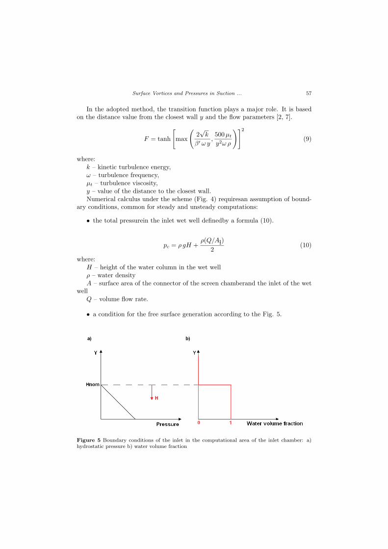
• a condition for the free surface generation according to the Fig. 5.

Figure 5 Boundary conditions of the inlet in the computational area of the inlet chamber: a)hydrostatic pressure b) water volume fraction


• the turbulence intensity at the level of 5 % (when I = 10) according to aformula:

I =µt

µd(11)

where: µt – turbulent viscosity, µd – dynamic viscosity

• mass flow of the outflow pipe: m = 24, 6 [kg/s],

• the zero gradient of the pressure in the direction of the main flow (this con-dition is assumed internally by the preprocessor of the ANSYS-CFX)

Unsteady conditions require additional settings:

• work area of the rotary screen to the total area of the screen is 74%

• assumed loss of pressure at the screen ∆p = 60 Pa,

• quadratic resistance coefficient:

KQ =

(∆p

∆x

)c2por (12)

where:

∆p – pressure loss at the porous surface

∆x – thickness of the screen (porous surface)

cpor – flow velocity of the liquid through the porous surface

• hydraulically smooth walls have been assumed,

• a logarithmicvelocity distributionon the wall has beenassumed – the so–calledwall function.

In the Fig. 6 below has been shown the diagram of dimensionless velocity u+ inthe function of dimensionless distance from the wall y+. To have the wall functionworking correctly, the first mesh node has to lie in the distance not smaller thany+ = 12 and not further than y+=200 (Fig. 7). For the value y+ <11 the meshnode lies in the laminar sub–layer and for y+ >300, beyond the boundary layer.

• a Courant number – is the basic criterion of the unsteady flow calculus definedas:

Courant =u∆t

∆x(13)

where:

u – the average velocity,

∆t – the time step,

∆x – the size of the mesh cell.


Figure 6 The range of values y+ [2]

Figure 7 The position of the first mesh node in the boundary layer in the area of logarithmicvelocity distribution (boundary layer) [2]

The scope of Courant number values, for the numerical computations, using theturbulence model SST, is not formulated. It is advisable to take such value, whichallows for obtaining solution with the assumed level of convergence [2]. In con-sideredmodels ofthe wet wellandthe formed suction intake, the value of Courantnumber is ranged in the scope (0.082.04) and for this value there was obtained theassumed level of convergence,

• the total time of computations: 30 [s],

• the time step: 0.001 [s],

• the minimal number of iterations for the given time step: 1,

• the maximal number of iterations for the given time step: 12,

• discretisation degree of the convective term: II order,

• the solution recording time step: 0.05 [s],


• tetrahedral mesh used in numerical computations,

• amount of control volumes in the case of the intake with barriers equals to 2,4mln, without barriers equals to ≈ 1,6 mln

• number of the mesh nodes for the intake with and without barriers equals to≈ 1 mln.

Geometry and the computation mesh for the intake with barriers is shown in theFig. 8 (variant 1). and for the intake without barriers in the Fig. 9 (variant 2).

Figure 8 Geometry and computation mesh for the model of the intake without barriers. Variant1

Figure 9 Geometry and computation mesh for the model of the intake with barriers. Variant 2


The analysis of obtained results of the unsteady computations quality consisted ofchecking the level of unbalanced mass flows and momentum in the control volumesof the mesh – a so called residuum [2] ( it determines the qualityof obtained results),which for the each of the results was in the range of. This level informs that the so-lution has a good convergence and which results will be validated with observationstaking place on the test stand.

3.3. A plan of the numerical calculus

Numerical computations of flow local parameters for the two construction variants,were carried out for the nominal liquid level in the intake of the facility (Fig. 1,(Hnom)m = 8, 3 m and (Qnom)m = 28050 m3/h).

Numerical computations validations were realized by results of flow measure-ments and observations on the test stand (chapter 4).

In the research of the model on the test stand, these values were correspondedwith following values: (Hnom)m = 0, 665 m and (Qnom)m = 88, 702 m3/h

Dimensionedvariant ofthe intakewith marked direction of the flow, measurementpoints of the pressure at the bottom of the wet well, curtain walls and the grid withthreads shown in the Fig. 10.

Figure 10 Model of the intake Variant 1 without the barrier, variant 2 with the barrier


Barriers (variant 2) were introduced after computations and research of the variant1. Barriers in the chamber were placed for the flow visualization in the neighborhoodof the suction intake. On the bottom of the intake were made measurement holesin order to measure pressures.

4. The test stand

4.1. Construction of the stand

The test stand enabled carrying out measurements and observations of values com-puted numerically.

Geometrical and flow parameters of the model were determined on the basisof the Froude (Fr) numbers equality condition for the facility and the model Fro= 1.094 ≈ Frm = 1.093. Because the Reynolds’ number Re > 3 *104 and theWeber number We > 120, far outweigh the critical values, it can be stated that thedynamic similarity condition between the object and the model is satisfied.

The test stand is shown in the Fig.11.

Figure 11 The test stand [3, 4] a)elevation of the test stand, b) view of the test stand, c) systemof the wet well (top view)


The test stand consists of: the screen chamber (1), inlet screens (2), the rotaryscreen (3), the wet well (4), the formed suction intake (5), the swirl meter (6), thePitot probe (7), pipelines (8), theflowmeter (9), the steam–waterseparation tank(10), the circulating pump (11), the main water tank (12), the delivery channel –model of the high–water source (13)

For validation of numerical computation results in the intake, there were usedresults of the observation of surface vortices, threads attached togrid nodes andpres-sure measurements inpressure holesat the bottom of the wet well (Fig. 10) madeduring the realization of measurements, discussed in [3, 4].

Measures and recordings of the pressure were made with the differential trans-ducer ofMobrey company – type 4301D2, with thepre–set measuring range -2500 ÷+2500 Pa, with the guaranteed tolerance ±5 Pa. The view of the apparatus shownin the Fig. 12.

Figure 12 Kit for measuringthe pressureat the bottom ofthe wet well

5. The comparative analysis of computation results and measurements

5.1. The pressure at the bottom of the suction intake

System for pressure measurements was adapted for measuring changes with a time–constant of several seconds. Because of the unsteady nature of the flow in the intake,there were compared average values of pressures computed numerically.

In the Tab. 1 there is a comparison of pressure values obtained from the mea-surement for (Hnom)m and (Qnom)m variant I.

Table 1Pressures in the pressure holes at the bottom of the wet well for(Hnom)m and (Qnom)m, variant I - measurementshole 2 hole 1 hole 3p [Pa] p [Pa] p [Pa]6394,72±5 6399,44±5 6395,45±5

Measured pressures in pressure holes 1–2–3 in the variant II of the formedsuctionintake were the same as in the variant I.


In the Tab. 2 are compared values of numerically computed values for eachpressure hole in the variant I of the formedsuction intake.

Time–averaged values of pressures computed numerically for Hnom, Qnom vari-ant I

Table 2Pressures in the pressure holes at the bottom of the wet well for(Hnom)m and (Qnom)m, variant Ihole 2 hole 1 hole 3p [Pa] p [Pa] p [Pa]6402,67 6410,8 6401,63

In the Ttab. 3 there are shown the time–averaged pressure values computednumerically for the nominal parameters of the intake operation Hnom, Qnom, variant2.

Table 3Numerically computed values of the pressure in measurement holeson the bottom of the wet well for (Hnom)m and (Qnom)m, variant 2hole 2 hole 1 hole 3p [Pa] p [Pa] p [Pa]6401.8 6406.23 6400.8

Runs of variables in time of computed pressures and their average values foreach hole shown in the Fig. 13 and Fig. 14 adequate for the intake without barriersand with barriers.

Figure 13 Characteristic values, temporary and mean in pressure holes 1 - 2 - 3 obtained innumerical computations. Variant 1


Figure 14 Characteristic values, temporary and mean in pressure holes 1 - 2 - 3 obtained innumerical computations. Variant 2

Figure 15 The distribution of numerically calculated pressures at the bottom of the formedsuction intake for the variant 1 and 2


Figure 16 Velocity distribution in the neighborhood of points 1-2-3 of the pressure measurementfor the variant 1 and 2

In Fig. 13 and Fig. 14 were also marked, with the vertical lines, boundaries oftransient phases from the steady flow to the RANS flow.

Measured differences of pressures see Tab. 1 variant 1, Tab. 2 variant 2, con-firmed using numerical computations Fig. 15.

Fig. 15 shows the equality of pressures in pressure holes ”2” and ”3”. In relationto the pressure in the pressure hole 1, they characterize with the less value. Thecause of smaller pressures are bigger values of the velocity in the neighborhood of”2” and ”3’ points, in relation to the velocity in the neighborhood of point 1 (Fig.16).

Velocity distribution in the neighborhood of points 1–2–3 is confirmed by thepressure distribution from measurements and numerical computations. In the point1 there occurs a velocity drop of both vortices in the neighborhood of this point.

5.2. The flow visualization of vortices in the wet well.

For work parameters of the wet well (Hnom)m and (Qnom)m two variants of thechamber construction (Fig. 10) there were performed:

• numerical computations of fluid flow parameters, on the basis of which, visu-alizations were made,


• observations of the flow on the test stand, with use of the inhabited pointwisecolorant and grids with threads installed in the wet well in the distance of 10cm from the inlet to the formed suctionintake (Fig. 10).

In Figs 17, 18 ,19 there are shown graphic illustrations of the numerical compu-tation and observations of the flow on the test stand.

Figure 17 Surface vortices in the wet well. Variant 1 (without barriers) a), b), c) visualizationof the flow based on numerical computations, d) observation of vortices on the test stand

During the flow through the wet well, there were noticed, appearing in the 30sec intervals, momentary (≈ 5 sec.) surface vortices without air bubbles under thewater surface. A surface condition in the wet well meets a standard of 1–2 classdue to the vortex classification Fig. 2.

Simultaneously, it can be confirmed the compatibility of the free surface of theliquid condition being a result of numerical computations and conditions observedon the test stand.

Due to the necessity of increase of the cooling water pump efficiency up tothe value of Qmax = 1.2Qnom,for instance in the case of the water temperatureincrease or the momentary power increase in a power unit, there were also performednumerical computations of the flow for Hnom and Qmax. In the Fig. 18 were showfree surfaces obtained as a result of numerical computations for Hnom and Qmax

and observations made on the test stand.During the flow there occur vortices of the class 3 in which dispersed air bubbles

constantly reach the inlet to theformed suction intake.In spite of the fact that the standard [1] does not allow the existence of the class

3 vortices at the free liquid surface in the wet well, curtain walls shown in the Fig.10b. were used.


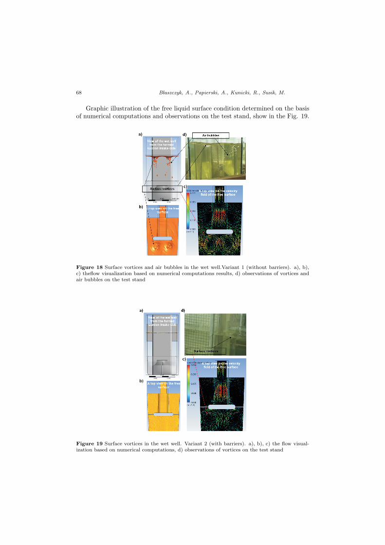
Graphic illustration of the free liquid surface condition determined on the basisof numerical computations and observations on the test stand, show in the Fig. 19.

Figure 18 Surface vortices and air bubbles in the wet well.Variant 1 (without barriers). a), b),c) theflow visualization based on numerical computations results, d) observations of vortices andair bubbles on the test stand

Figure 19 Surface vortices in the wet well. Variant 2 (with barriers). a), b), c) the flow visual-ization based on numerical computations, d) observations of vortices on the test stand


Presented condition of the free liquid surface fulfills requirements of the class 1vortices. There were also performed visualizations of the flow in the neighborhoodof the outlet to the inlet chamber. In the Fig. 20 is shown the numerically computedvelocity distribution in the plane perpendicular to the direction of the flowin thedistance of 10 cm from the suction chamber. In the neighborhood of the front walland the inlet to the formed suction intake there was noticed a backward flow.

Figure 20 Velocity vectors distribution in the neighborhood of the inlet to the suction intake

Figure 21 View of the grid with threads

Obtained numerical computation based distributions were confirmed by the obser-vation of threads attached to the grid (Fig. 21).

6. Conclusions

Conclusions andfinal remarkscan berepresented as following points:

1. Changes, during numerically computedpressures, prove the unsteadynatureofthe flow inthe wet well(Fig.13, Fig. 14),

2. Minimal differences between computed and measured mean pressures arisefrom:


• the pressure measurement uncertainty, includingthe dynamics ofthe mea-surement system,

• participation of the dynamic pressure in the value of measured pressure.

From the comparison of tables T-1 and T-2, T-1and T-3 it follows that for eachpressure hole, the pressure is smaller than averaged pressures computed numerically.

From the Fig. 14 it follows the equality of pressures in pressure holes 2 and 3.In relation tothepressurein the hole 1theyare characterized bylower values. A

cause of less pressure values are larger velocities in the neighborhood of 2 and 3points in relation to velocities in the neighborhood of point 1 (Fig. 16).

1. In the plot Fig. 13, Fig. 14 there can be distinguished three phases of thepressure change:

• Phase 1. Change of the pressure is characteristic for the transition fromthe steady to RANS flow.

• Phase 2. Initially pressures amplitudes dramatically increase and sec-ondly randomly decrease.

• Phase 3. In this phase fluctuation of the pressure are stabilizing what ischaracteristic of the RANS flow.

2. The condition of free surfaces in the wet well, based onnumerical computa-tions, is similar to the free surface condition observed on the test stand (Fig.17, 18, 19).

3. For nominal parameters of work of the intake (Hnom)m and (Qnom)m the freesurface condition meets the class 1 – 2 according to the vortices classificationin [1].

4. In the case of work parameters of the chamber (Hnom)m and (Qmax)m, thereoccurred surface vortices and air bubbles constantly flowing into the formedsuction intake. According to the vortices classification [1] these are vorticesof the 3 – 4 class.

5. Introduction of curtain walls caused a drop of vortices of the class 3 to theclass 1.

6. The proposed numerical calculus algorithm may be used in the analysis ofunsteady flows in pumpintakes.

References

[1] American National Standard for Pump Intake Design, ANSI/HI 9.8-1998. Hy-draulic Institute. 9 Sylvan Way, Parsippany, New Jersey 07054-3802, www.pumps.org

[2] ANSYS CFX, Release 12.1: Theory Manual, 2001.

[3] B laszczyk, A., Najdecki, S., Papierski, A., Staniszewski, J.: Modelexaminations of the suction intake of the cooling water pump 180P19 on the teststand no. 8 for a unit A 460MW in Ptnow Power Plant, Report of the work stage I,Archives of the Institute of Turbomachinery TU of Lodz, 1542, 2006.


[4] B laszczyk, A., Najdecki, S., Papierski, A. and Staniszewski, J.: Modelexaminations of the suction intake of the cooling water pump 180P19 on the teststand no. 8 for a unit A 460MW in Ptnow Power Plant, Report of the work stage II,Archives of the Institute of Turbomachinery TU of Lodz, 1546, 2006.

[5] Karassik, I. J., Messina, J. P., Cooper, P. and Heald, Ch. C.: Pump Hand-book, Third Edition, McGraw–Hill, New York, 2001.

[6] Kazimierski, Z. Numeryczne wyznaczenie trojwymiarowych przep lywow turbulent-nych, Maszyny Przep lywowe, Wroc law, Vol. 11, 1992.

[7] Kuczkowski, M.: Numeryczny model turbulencji przep lywu przez zagiecie przewoduz wykorzystaniem metody LES, Ph. D. thesis, Lodz, 2007.

[8] Kunicki, R.: Numeryczne i doswiadczalne badania przep lywow nieustalonych w ko-morach wlotowych pomp, Ph. D. thesis, Lodz, 2011.

[9] Li, S., Lai, Y., Weber, L., Silva, J.M. and Patel, V.C.: Validation of a 3DNumerical Model for Water Pump Intakes, Journal Hydraulic Research, 42(3), 282–292, 2004.

[10] Mahesh, K., Constantinescu, S. G. and Moin P.: A Numerical Method forLarge Eddy Simulation in Complex Geometries, Journal of Computational Physics,197(1), 215–240, 2004.

[11] Menter, F.R.: Multiscale model of turbulent flows, AIAA, 24th Fluid DynamicConference, 1993.

[12] Rajendran, V. P., Constantinescu, S. G. and Patel, V. C.: ExperimentalValidation of Numerical Model of Flow in Pump–Intake Bays, Journal of HydraulicEngineering, 125(11), 1119–1125, 1999.

[13] Tullis, J.P.: Modeling in design of pumping pits, Journal of the Hydraulic Division,Vol. 105, No. HY9, P. 1053–1063, 1979.

[14] Zaino, A.: Wp lyw parametrow konstrukcyjnych na zjawiska przep lywowe w ko-morach wlotowych zamknietych duzych pomp wirowych, Technical University ofWroc law, 1994.


Documents

Surface Vortices and Pressures in Suction Intakes of ...kdm.p.lodz.pl/articles/2012/6_B_P.pdf · Mechanics and Mechanical Engineering Vol. 16, No. 1 (2012) 51{71 ⃝c Technical University