Embed Size (px)
Citation preview
SURFACE TRANSFORMATIONS*
BY
F. R. BAMFORTHf
In a paper written by BirkhoffJ on the Problem of Three Bodies, he
reduced the study of a certain phase of this celebrated problem to the study
of a surface transformation which was the product of two surface trans-
formations each of which represented the reflection, in a curve lying in a
surface, of the surface into itself. It is the purpose of this paper to make
a start on the study of such surface transformations in general.
In the first section are studied surface transformations of period two,
and it is shown that when a suitable coordinate system has been chosen,
any such transformation may be represented by one and but one of the
following systems of equations :
Ml = M, Mi = — M, M! = M,
vi = v; Vi = — v; V\ = — v;
in which the point («i, Vi) denotes the transform of the point (u, v).
In the remaining sections, surface transformations are discussed which
are the product of two transformations, each of which, when a suitable
coordinate system has been selected, can be represented by equations of
the third type in (1).
I. Transformations of period two
This section will be concerned with real, one-to-one, analytic transforma-
tions of a surface Z into itself, of such a character that after the same trans-
formation has been performed twice in succession all the points of the
surface are in the same positions with respect to fixed axes as they were before.
These transformations are called transformations of period two, and we shall
study the movement under such transformations of the points of the surface Z
in a neighborhood of a point which is invariant.
In a neighborhood of such an invariant point the equations representing
the transformation may be written in the form
(2) Mi = au + bv + ■ • ■ , Vi — cu + dv + ■ ■ ■ , ad — be ^ 0,
* Presented to the Society, December 27, 1929; received by the editors February 28, 1930.
f This paper was partially prepared while the author was a National Research Fellow.
t G. D. Birkhoff, Rendiconti del Circolo Matemático di Palermo, vol. 39.
417
License or copyright restrictions may apply to redistribution; see http://www.ams.org/journal-terms-of-use

418 F. R. BAMFORTH [July
after a proper choice of coordinate system has been made. For this system
of coordinates the origin is the invariant point and the series on the right
hand sides of the equations (2) are convergent for u and v sufficiently small
in absolute value. By means of a real, linear change of variables, the equa-
tions (2) of the transformation are equivalent to equations which will have
one of the following forms:
(3) «i = au + • • • , vi = av + • • • , a 9¿ 0;
(4) Hi - V H-, vi = ßu + Sa + • • • , ß j¿ o,
where the dots indicate terms of degree greater than one.
Let us now discuss transformations which may be represented by equa-
tions of the form (3). If we denote the transform of (wi, Vi) by (u2, v2), from
the fact that the transformation is of period two, it follows that
« = «2 = a«i + • • • = a2u + • • • , v = v2 = avi + • • • = a2v + • • • ,
whence a=±l. Suppose first that a = l. The transformation may be
represented by
«i = u + a20u2 + anuv + a02v2 + • • • ,
Vi = v + b20u2 + buuv + bo2v2 + • • • .
Since the transformation is of period two
m = «2 = «i + û2o«i2 + anuiVi + a02î>i2 + ■ • •
= « + 2o2o«2 + 2anuv + 2a02»2 + • • • .
From this identity it follows that all the a<,- are zero, and from the corre-
sponding one in v it follows that all the by are also zero. Hence, when a
transformation of period two can be represented by equations of the form
(3) with a = 1, it is the identity transformation.
Transformations represented by equations of the form (3) with a = — 1
will be called "rotation transformations" on account of the fact that the
simplest example of equations of this form, i.e., «i= — u, Vi= — v, represents
a rotation through 180° when the coordinate system is rectangular. We shall
now reduce the equations (3) of a rotation transformation to a simpler form.
To this end let us write these equations in the form
(5) Mi = - m + U(u,v), Vi= -v + V(u,v),
where U(u, v) and V(u, v) have no terms of first degree in u and v. On account
of the periodicity of the transformation,
m = m2 = — Mi + ¡7(mi,î>i) = m — U(u,v) + Z7(Mi,»i),
v = v2 = — »i + V(ui,vi) - v — V(u,v) + V(ui,vi),
License or copyright restrictions may apply to redistribution; see http://www.ams.org/journal-terms-of-use

1930] SURFACE TRANSFORMATIONS 419
whence
U(u,v) = U(ui,vi), V(u,v) = V(ui,vi).
Hence the equations (5) are equivalent to the equations
«i — %U(ui,Vi) = — u + \U(u,v),
vi - J7(«i,»i) = - v + ?V(u,v).
Under the change of variables
M* = M — \U(U,V), V* = V — %V(U,V),
these equations are evidently transformed into
Mi* = — M*, V* = — V*,
from which form the structure of the transformation is evident.
If a transformation of period two is represented by equations of the
form (4),
u = u2 = Vi+ • • • = ßu + 8v + • • ■ ,
v = v2 = ßui + ôvi + ■ ■ ■ = ßv + 8ßu + 82v + ■ ■ ■ ,
whence ß = l and 5 = 0. The equations representing such a transformation,
by means of a suitable change of coordinate system, may be of either of
the two forms
(6) Mi = »+••• , Vi = u+ • ■ ■ ,
or
(7) Mi = M + ■ • ■ , V! = — V + ■ ■ ■ .
The equivalence is readily seen if the coordinates are considered as rectangu-
lar coordinates in the plane and a rotation of axes through an angle of 45°
is performed. Since the simplest example of equations of the form (7)
representing such a transformation of period two, i.e., ux = u, Vi= —v, repre-
sents a reflection in the u axis, we shall call any transformation of period
two which can be represented by equations of the form (6) or (7), a "reflec-
tion transformation."
Let us write the equations (7) in the form
(8) «i = « + U(u,v), vi « - t» + V(u,v).
Here, on account of the periodicity of the transformation,
U(u,v) = - U(ui,v0, V(u,v) = V(u1)Vl).
Hence the equations (8) are equivalent to the equations
License or copyright restrictions may apply to redistribution; see http://www.ams.org/journal-terms-of-use
420 F. R. BAMFORTH lluly
Mi + ÍU(Ui,Vi) = u + %U(u,v),
vi — hV(ui,vi) = — v + \V(u,v),
from which it follows immediately that this transformation may be repre-
sented by the equations
(9) uf = u*, vi* = - v*,
where
u* = u + ?U(u,v), v* = v — %V(u,v).
Here, as in the case of rotation transformations, the form (9) tells us every-
thing that we wish to know about the transformation.
When a transformation of the reflection type is represented in a neighbor-
hood of an invariant point by equations of the form (9), we shall say that
the u*v* system of coordinates is a "normal system" for the transformation.
Now it is evident that there are infinitely many normal coordinate systems
for any one such transformation. In fact, if we make a reversible change of
coordinates defined by the equations
(10) m* = f(w,z), v* = g(w,z),
a sufficient condition that the new system of coordinates be a normal system
for this transformation is that
(11) f(i», - z) =/(w,z), g(w, - z) = - g(w,z).
This is a consequence of the fact that if (11) be true, Wi = w, Zi= — z is a
solution of the pair of equations
f(wi,zi) = f(w,z), g(wi,zi) = - g(w,z).
By way of summarizing this first section, we may say that every transfor-
mation of period two, in a neighborhood of an invariant point, after a suitable
choice of coordinate system has been made, may be represented by one and but
one of the following systems of equations :
Ui = U, Ui = — U, Mi = M,
Vi = v; vi = — v; vi = — v.
II. Product transformations
In Birkhoff's paper on the Problem of Three Bodies, a transformation
of a surface into itself arose which was the product of two transformations
each of which was of the reflection type. The object of this and the succeeding
sections of this paper is to study such transformations in the neighborhood
License or copyright restrictions may apply to redistribution; see http://www.ams.org/journal-terms-of-use
1930] SURFACE TRANSFORMATIONS 421
of a point which is invariant under each of the component transformations
of period two.
In the notation we shall use, the script letters %, and S will stand for
transformations of the reflection type of a surface Z into itself, and the script
letter 13 will stand for the product transformation 13=5^8 • In a neighbor-
hood of a point which is invariant under the transformation S, by choosing
a normal system of coordinates for this transformation, it may be represented
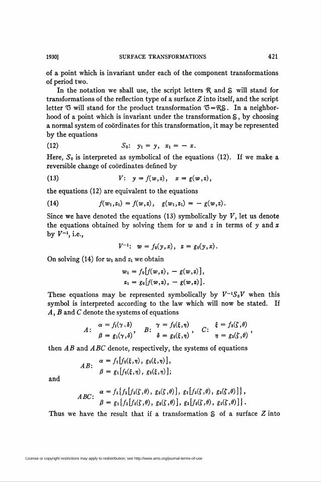
by the equations
(12) S0: yx = y, xx = — x.
Here, S0 is interpreted as symbolical of the equations (12). If we make a
reversible change of coordinates defined by
(13) V: y=f(w,z), x = g(w,z),
the equations (12) are equivalent to the equations
(14) f(wi,zi) =f(w,z), g(wl,z1) = - g(w,z).
Since we have denoted the equations (13) symbolically by V, let us denote
the equations obtained by solving them for w and z in terms of y and x
by V-\ i.e.,
V~u. w = fo(y,x), z = go(y,x).
On solving (14) for wx and zx we obtain
wi = fo[f(w,z), - g(w,z)],
zi = go[f(w,z), - g(w,z)].
These equations may be represented symbolically by V~lSaV when this
symbol is interpreted according to the law which will now be stated. If
A, B and C denote the systems of equations
a a=fx(y,ô) b y=f2(£,v) í=/3(r,0)
ß = gi(y,8)' 8 = g2(H,ri)' n = gti,e)'
then AB and ABC denote, respectively, the systems of equations
tl, « = /i[M£,>/), gi(i,■»))],AB:
ß = gi\f*(Z,v), «»(É.i?)];and
.„ « =/i{/i[/iM, gi(f,«)], gi[f*(S,e), gz(t,e)]},A .dC : , , ,,
ß = íi{/i[/iM, «.o:,»)], gi[/iM, fi(r,e)]}.Thus we have the result that if a transformation S of a surface Z into
License or copyright restrictions may apply to redistribution; see http://www.ams.org/journal-terms-of-use
422 F. R. BAMFORTH [July
(17)
itself be denoted by the equations So of (12), and if a change of coordinate
systems denoted by the equations V of (13) takes place, the transformation
S is denoted in the new system of coordinates by the equations V^SoV.
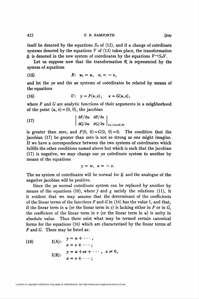
Let us suppose now that the transformation 1{ is represented by the
system of equations
(15) R: Mi = m, vi = — v,
and let the yx and the uv systems of coordinates be related by means of
the equations
(16) U: y=F(u,v), x=G(u,v),
where F and G are analytic functions of their arguments in a neighborhood
of the point (u, v) — (0, 0), the jacobian
dF/du dF/dv
dG/du dG/dv (u,»)-«>,o)
is greater than zero, and F(0, 0)=G(0, 0)=0. The condition that the
jacobian (17) be greater than zero is not so strong as one might imagine.
If we have a correspondence between the two systems of coordinates which
fulfills the other conditions named above but which is such that the jacobian
(17) is negative, we may change our yx coordinate system to another by
means of the equations
y = w, x = — z.
The wz system of coordinates will be normal for S and the analogue of the
negative jacobian will be positive.
Since the yx normal coordinate system can be replaced by another by
means of the equations (10), where/ and g satisfy the relations (11), it
it evident that we may assume that the determinant of the coefficients
of the linear terms of the functions F and G in (16) has the value 1, and that,
if the linear term in u (or the linear term in v) is lacking either in F or in G,
the coefficient of the linear term in v (or the linear term in u) is unity in
absolute value. Thus there exist what may be termed certain canonical
forms for the equations (16) which are characterized by the linear terms of
F and G. These may be listed as:
y = m + • • • ,(18) 1(A):
x = »+••• ;
y = m +fl» + • • • , s^O,KB):
x = i)+ • • • ;
License or copyright restrictions may apply to redistribution; see http://www.ams.org/journal-terms-of-use

19301 SURFACE TRANSFORMATIONS 423
11(A) :
1KB):
III:
IV:
V:
VI:
y = v+■ • ■ ,
x = - m + • • • ;
y = au + »+•••, «7*0,
x = - m + • • • ;
y = M+ • • • ,
x = a« + »+•■• , a 5¿ 0;
y = »H-,x = — m — a» + • • • , a ?* 0;
y = aioM + a0i» + • • • ,
x = JioM + boiV + • • • , aioaoïbioboi > 0;
y = aïo« + a0i» + • • • ,
x = JioM + boiV + • • • , aioaoïbioboi < 0.
The equations 1(B), 11(B), III and IV may be assumed to be in a still
simpler form. Consider, for example, the equations 1(B), and make use of
the change of coordinates
y = y*, « = «*,
x = x*/(2a); v = v*/(2a).
Evidently the transformed equations of 1(B) have the form
y* = m* + \v* + • • • ,
Since analogous transformations may be employed in the other cases, it is
evident that we may assume that wherever "a" appears in the equations (18)
we may write %. This choice of constant "a" gives a particularly simple
form to the canonical forms which will be given later of the equations re-
presenting transformations 13.
Let us now consider the transformation 13 of the surface Z into itself
which is the product of the transformations 'R. and S, i.e., 13=^8, which is
to mean that the transformation S is followed by the transformation <r\.
We shall first discuss one of the properties of this transformation 13 which
can be readily proved out of the fact that each of the transformations R.
and S is of period two. Let the symbol 5 represent the equations of the trans-
formation § in the uv system of coordinates which is normal for the trans-
formation R. represented by the equations (15). On account of the equations
(16) we see that symbolically S = U-lS0U, where S0 is given in (12). If T
License or copyright restrictions may apply to redistribution; see http://www.ams.org/journal-terms-of-use

424 F. R. BAMFORTH [July
represents the equations of the transformation 13 in the uv system of coordi-
nates, evidently T = RS. If we denote the identity transformation by /,
we have symbolically
SS = I, S = S-1, R = R-1, T = RS, TSR = RSSR = I,
2-1 = SR = SRSS-1 = RRSR = STS-1 = R-^TR.
It is this last equation, T~l = R_1TR, which we wish to examine more closely.
Since a change of coordinate systems denoted by V changes the equations
T into F"T7 we see that the inverse transformation of 13 is represented in
the uv system of coordinates by the same equations as the transformation 13
after the change of coordinate systems denoted by R has taken place. Thus,
if the equations T are
t ux = axu + a2v+--- ,
Vi = bxu + b2v + ■ • ■ ,
and if we perform a change of coordinates denoted by
(20) R: m = s, v = - /,
obtaining thereby
sx = axs — a2t + ■ • ■ ,(21) R-'TR: .
tx = — bxs + b2t + ■ • ■ ,
in the uv system of coordinates 13~1 is given by
m = aiMi — a2vx + ■ ■ ■ ,(22) 7*-1:
V = — ÔiMi + ¿2îii + • • • .
Thus, observing the movement of the points of the surface Z under the
transformation 'S-1 is equivalent to observing the movement of the points
of the reflection of the surface Z under 13 in a mirror which is plane for
the uv system of coordinates. We shall make use of this fact later on in the
discussion.
Let us now return to a further consideration of the normal forms (18)
of the equations of the change of coordinate systems. The transformation S
in the uv system is given by
(23) F(mi,vx) =F(u,v), G(ux,vx) = - G(u,v).
Hence the transformation 13 is given by
(24) F(ux, - vx) = .F(m,70, G(mi, - vx) = - G(u,v).
The normal forms for the equations T which correspond to the normal forms
License or copyright restrictions may apply to redistribution; see http://www.ams.org/journal-terms-of-use

1930] SURFACE TRANSFORMATIONS 425
(18) are the following
1(A):
KB):
11(A):
11(B):
III:
IV:
(25)
VI:
Ml = M + • • • ,
vi = v + ■ ■ ■ ;
Mi = M + V + • • • ,
vi = v + • • • ;
Mi = - M + • • • ,
vi = - v + • • • ;
Ml = - M + • • • ,
vi = — m — v + • • • ;
Ml = M + • • • ,
vi = m + v + • • • ;
Mi = — M — V + ■ • • ,
vi = —»+•••;
Mi = a« + /3d + • • • ,
»i = yu + av + • • • , 07 > 0, a ^ 0;
«i = «m + j8» + • • • ,
Vi = yu + av + • • • , 07 < 0;
where a = aiab0i+aoibio, ß = 2a0ib0i, 7 = 2ai0öio, a2—07 = 1. Evidently, each
of the type sets of equation in (25) is but an example of
Mi = au + ßv + ■ • • ,
(26) T:Vi = yu + av + • • • ,
where a, ß or y may have the value zero.
Thus we have obtained the result that every transformation which is the
product of two transformations of the reflection type, in a neighborhood of a
point which is invariant under each of the component transformations, can be
represented in one and only one way by equations which are of one of the types
displayed in (25).
III. Invariant directions and simple examples
Let us now inquire into the possibility of there being directions through
the origin which are either invariant under T or are rotated through 180°.
From (26) when aßy^O we obtain at (u, v) = (0, 0) for du/dv finite and differ-
ent from —a/7
License or copyright restrictions may apply to redistribution; see http://www.ams.org/journal-terms-of-use

426 F. R. BAMFORTH LTuly
-<t)'dux du adu + ßdv du
dvx dv y du + adv dv duy — + a
dv
If du/dv= —a/7 or is infinite, then dv/du^—a/ß, since a2—ßy = l, and
dvx dv \du/
dux du dva + ß —
du
Hence du/dv remains unchanged by T if and only if
(27) ß(dv)2 - y(du)2 = 0.
Now consider the case where a = 0. Then ßy^Q, and
dMi ß dv
when dv/du is finite anddvx y du
dvx y du
dux ß dv
when du/dv is finite. Thus the invariant values of du/dv are given by (27).
In a similar manner it can readily be shown that the invariant values of
du/dv for ß = 0 or y = 0 are also given by (27).
Thus we find that for all transformations of the types 1(A) and 11(A),
all slopes through the origin are invariant; for all transformations of the types
1(B), 11(B), III and IV there are two coincident invariant slopes which are
the only ones; for all transformations of the type V there are two distinct in-
variant slopes which are the only ones; and for transformations of the type VI
there is no invariant slope.
It would, perhaps, be useful in clarifying our ideas to give at this point
a short discussion of transformations of the different fundamental types in
which only linear terms appear on the right hand sides of the equations (25).
Each of these transformations is area preserving since the jacobian of the
functions on the right hand sides of each pair of these equations is 1.
The transformation ux = u, vx = v, which is of type 1(A), is evidently the
identity transformation under which every point is an invariant point.
For the transformation
(28) Mi = m + v, vx = v,
License or copyright restrictions may apply to redistribution; see http://www.ams.org/journal-terms-of-use

1930] SURFACE TRANSFORMATIONS 427
of type 1(B), the u and y axes are coincident while the equation of the
x-axis in the Mü-system of coordinates is given by u+$v = 0. The only in-
variant curve for this transformation which passes through the origin is
the «-axis, and since v is an invariant function, the points move parallel to
the «-axis under the transformation 15. Moreover, this invariant curve is
made up of invariant points. It is easily verified that this transformation
has the origin as a hyperbolic, unstable,! invariant point, since for v>0,
ux — u>0, and for v<0,ux—u<0. In fact, if any neighborhood of the origin
be taken, it is evident that the only points which remain in the neighborhood
under the indefinite iteration of T and of T~l are those lying on the «-axis
which are invariant points.
The transformation ux = — u, vx = —v, of type 11(A), is a rotation through
180°. Thus every straight line through the origin is invariant and the
points on it are reflected in the origin, which is an isolated, hyperbolic,
stable, invariant point for 15. The x and the u axes are coincident, as are also
the y and the v.
For the transformation «i= — u, vx= —u—v, of type 11(B), the y and v
axes are coincident and the equation of the «-axis in the «v-system of coordi-
nates is given by %u+v = 0. The only invariant curve through the origin
is the a-axis on which all the points are reflected in the origin by 13. The
origin is a hyperbolic, unstable, invariant point.
For the transformation mi=m, vx = u+v, of type III, the x and v axes are
coincident and the equation of the y axis is $u+v = 0. The origin is a hyper-
bolic, unstable, invariant point, and the only invariant curve through it is
the v axis. The discussion of the simple transformation of type IV is obviously
similar to that of type III.
For the transformation
(29) ux = au + ßv, vx = yu + av, a > 0, ß > 0, y > 0,
of type V, ßv2—yu2 is an invariant function which is zero on the two in-
variant lines ßv2—yu2 = 0 through the origin, which is therefore a hyperbolic,
invariant point. The u axis bisects the angle between these two invariant
lines. Let us examine the movement under 15 of the points on these invariant
lines. Let (u, v) be any point on the invariant line u = v(ß/y)112. Then
«i = au + ßv = (a + (ßy)ll2)u,
vx = yu + av = ((ßy)112 + a)v.
t Definitions of certain technical terms used in the discussion of this paper will be found in a
paper by G. D. Birkhoff, Acta Mathematica, vol. 43: conservative transformation, p. 2; formal con-
servative transformation, p.22; quasi-invariant function, p.2; stable and unstable invariant points,
p. 5; formal invariant curve through origin, p. 26; hypercontinuous invariant curve, p. 67; elliptic
and hyperbolic invariant points, p. 26. This paper will be referred to hereafter as B.
License or copyright restrictions may apply to redistribution; see http://www.ams.org/journal-terms-of-use

428 F. R. BAMFORTH [July
Now (a+(ßy)112) (a-(ßy)1'2) = l. Hence a + (ßy)112 is positive and either
is greater than 1 or less than 1. If a+(07)1/2>l, the points on this invariant
line will recede from the origin on iteration of 13 and if a+(ßy)ll2<l the
points will approach the origin on iteration of 13. But if a+(ßy)ll2<1,
a — (ßy)U2>\, and hence the points on one of the invariant lines recede from
the origin on iteration of 13 and the points on the other invariant line ap-
proach the origin on iteration of 13. This shows that the origin is an unstable
invariant point.
Suppose that for the transformation represented by (29) we make a
change of coordinates which takes these invariant curves into the axes.
Then the equations (29) become üi = bü, Vi = cv, ¿>>1, 0<c<l, which shows
that no other invariant curves exist for the transformation (29) than those
already mentioned.
The transformation which is the same as (29) with the exception that
a <0, can be discussed in a manner similar to that in which we have discussed
(29). In this transformation the points on one of the invariant lines recede
from the origin on iteration of 13 but oscillate about the origin in so doing.
By this is meant that the origin always separates a point on this invariant
line from its image under 13. The points on the other invariant line approach
the origin under iteration of 13 but also oscillate with respect to it.
For the transformation ui = au+ßv, Vi = yu+av, ß>0, 7<0, which is of
the type VI, as has already been proved there is no invariant slope through
the origin. Hence there is no invariant curve through it and the origin is an
elliptic, invariant point. In this case the function ßv2—yu2 is an invariant
function which shows that the origin is a stable invariant point.
Since all the simple transformations which we have just been discussing
preserve areas and hence have invariant integrals, it would seem that it
would be advantageous to link that classification which we have given for
transformations 13=ír\S with that given by Birkhoff in his paper in the Acta
Mathematica. It will be assumed that the reader has this paper before
him; the classification is on page 4. We shall designate the types of problems
which we are studying by 1(A), 1(B), etc., and those which Birkhoff studied
by I', I", etc., as he did. With this notation in mind, it is evident that we
have the following correspondence based upon the coefficients of the linear
terms in the equations of the transformations: I(A)~II", 1(B)~III',
ii(A)->n"', ii(b)~iii", m~iir, iv~ni", v(«>o)~r, v(«<o)~i",VI(a = 0)~II'", VI(a5¿0)~II'or II'". Reference will be made to this
correspondence from time to time. When interpreting this correspondence
we should remember the properties of the u and v axes of coordinates as used
in this paper, made clear by the equations (15).
License or copyright restrictions may apply to redistribution; see http://www.ams.org/journal-terms-of-use

1930] SURFACE TRANSFORMATIONS 429
IV. Formal invariant series
The question of the existence of real, formal series which are invariant
under the equations representing a transformation 15 is important for at
least two reasons. If there is such a series which is convergent, by setting
it equal to a constant we obtain a curve which is invariant under 15. Hence
we can study the transformation by studying the totality of such invariant
curves. On the other hand, if there does not exist any series which is con-
vergent, but there does exist one that is divergent for all sets of values of
the variables different from (0,0), it can be used in many cases to reduce the
equations representing the transformation to a simpler form and to prove
the existence or non-existence of real invariant curves through the origin
which is assumed to be an invariant point of the transformation. Hence
we shall search for series which are formally invariant under T = RS.
Let us now recall that T~l = R~1TR=S~1TS, which means that the equa-
tions giving the inverse transformation 15_1 are the same in form as those
for the transformation 15 itself after a change of variables has taken place
in which the equations of the change of variables are those of the transforma-
tion % or of the transformation S ■ In this connection, let us return to the
consideration of the equations (19), (20), (21) and (22), and the discussion
given concerning them. Thus we see that, if H(u, v) is a formal invariant
series under (19), H(s,—i) is invariant under (21) and hence H(u,—v) is
invariant under (22). Thus, if the series H(u, v) is invariant under T, the
series H(u,—v), H(u, v) +H(u,—v) and H(u, v) —H(u,—v) are too; and every
series which is invariant under T is the sum of an invariant series which is
even in v and an invariant series which is odd in v. This follows immediately
from the fact that if a series is invariant under T it is also invariant under
t-\
Furthermore, if the transformation 15 is written in the variables y and x
by means of the equations (16) it is readily seen that every series that is
formally invariant is the sum of an invariant series which is even in x and
an invariant series which is odd in x.
Now let us consider the equations (24) for the transformation 15. These
equations may be written in the form
F(u,v) = a0(u) + ax(u)v + a2(u)v2 + a3(u)vs + • • •
= a0(ux) — ax(ux)vx + a2(ux)vx2 — a3(ux)vx3 + ■ ■ ■ ,
G(u,v) = b0(u) + bx(u)v + b2(u)v2 + b3(u)v3 + ■ • •
= - io(wi) + bx(ux)vx - b2(ux)vx2 + b3(ux)vx3 — ■ ■ ■ .
From the reasoning given in the preceding paragraph it is evident that if
there is a formal series which is invariant under T there is one, K(y, x),
License or copyright restrictions may apply to redistribution; see http://www.ams.org/journal-terms-of-use

430 F. R. BAMFORTH [July
in the variables y and x which is invariant under T and is even in x and con-
sequently in G(u, v) when the variables y and x are replaced by the functions
F(u, v) and G(u, v) of (16). Hence from (24),
K[F(ui,vi),G(ui,vi)] = K[F(u,v),G(u,v)] = K{F(uu - vi), -G(ui, - vt)].
But K is an even function of G by hypothesis. Hence
K[F(ui,vi),G(ui,vi)] = K[F(ui, - Vi),G(uu - vi)],
whence K is even in v\, and hence, when it is expressed in terms of u and v,
even in v. In an analogous manner it can easily be proved that any invariant
series which is odd in x in the yx-system of coordinates is odd in î; when
written in the Mü-system of coordinates. Since the square of an invariant
series which is odd in v is an invariant series which is even in v we see that
there exists a series which is formally invariant under T if and only if there
exists such a series which is even in v.
We shall now examine transformations 13 to find out whether formally
invariant series can exist, and we shall limit the discussion at first to the cases
in which the transformations are of the type V, or VI with a^O. Since
we have shown that there exists a formally invariant series for such a
transformation if and only if there exists one which is even in x, and hence,
as has been shown, even in v, we shall try to show that, for the cases under
consideration, there exists a formally invariant series which is even in x and,
when expressed in terms of u and v, is even in v.
It is readily provable that if there exists an invariant series it can not
have any terms of the first degree in u or in v. Hence we shall start with
second degree terms. Let us write the equations (30) in the form
F(u,v) = oioM + aoiv + a20u2 + anuv + a02v2 + • • •
= öioMi — a0i»i + fl2o«i2 — aiiMitii + Oo2vi2 + • • • ,
G(u,v) = biou + boiv + &2o«2 + bnuv + ¿>02fl2 + • • •
= — ¿ioMi + ¿oifll — ¿>20Mi2 + bnUiVi — io2fli2 + • • • .
Now from the way in which the series F(u, v) and G(u, v) are transformed
by T we see that our invariant series which is to be even in x and consequently
in G must be such that when F and G are expanded in terms of u and v no
term of odd degree in v appears. In so far as the second degree terms are
concerned, except for a constant factor, there is only one combination of
F and G which is even in v and invariant under T up to terms of degree three,
and this is
(32) bioboiF2 — aoiaioG2.
License or copyright restrictions may apply to redistribution; see http://www.ams.org/journal-terms-of-use

1930] SURFACE TRANSFORMATIONS 431
This expression transforms under T in the same manner as do F and G2, and
has no term of the second degree in u and v which is odd in v. The method
which we shall use to build up our formally invariant series consists in adding
to the function (32) a function of the third degree in F and G which is even
in G and which is such that the resulting sum contains no term of the third
degree in u and v which is odd in v; and then adding to this sum a function
of the fourth degree in F and G which is even in G and which is such that
this last sum will contain no term of the fourth degree in u and v which is
odd in v; this process being continued so long as any terms of odd degree
in v remain in the sum. Now the series (32) is invariant up to its terms of
the third order; the series obtained from (32), after the first addition has
been made to it, will be invariant up to terms of the fourth order; and so on.
Thus, if we can prove that at no stage does the above outlined process of
adding functions break down, we shall have established the fact that there
exists an invariant series for transformations 15 of the types V and VI
with a?¿0.
Let us now investigate what we need to prove in order to show that this
process does not break down at any stage. Suppose we wish to eliminate
terms of odd order in v in the group of terms of the rth degree in u and v.
To do this we may employ a sum of the form
(33) aoGr + ßoG^F2 + ■ ■ ■ + voFr
if r is even, and of the form
(34) aoG*-W + ßoG'-W + ■ ■ ■ + r,0Fr
if r is odd.
Let us first consider the case when r is odd. When a sum of the form (34)
is employed, we see that to determine the (r+l)/2 multipliers a0, ßo, • • • , Vo,
we shall have (r + l)/2 linear algebraic equations. Hence, if we are to show
that in every case we shall be able to solve these equations we shall have to
show that the determinant of the coefficients of a0, • ■ ■ , j?0 in these equations
is different from zero. Proving this is equivalent to proving that if the func-
tion (34) is even in v up to terms of the (r+l)th order, a0=ßo= • • ■ =770 = 0.
Evidently, in this proof only the linear terms of F and G will be involved.
Hence let us define
„ , F0(u,v) = dioM + a0iv,
(35)Go(u,v) = bxou + boxv,
where F0 and G0 are thus the linear terms of F and G, respectively. Hence
axobox — aoxbxo may be assumed to be 1. Consequently the transformation 15o,
License or copyright restrictions may apply to redistribution; see http://www.ams.org/journal-terms-of-use

432 F. R. BAMFORTH [July
which is defined by
. Mi = au + ßv, a = aïoôoi + aoi&io, ß = 2a0iboi,(36) in;
Vi = yu + av, 7 = 2ai06io,
and hence is the transformation obtained by using only the first degree terms
in the equations T of (26), is the transformation defined by
Fo(ui, - vi) = F0(u,v),
Go(ui, — vi) ~ —Go(u,v).
Since we are considering only transformations 13 of the types V and VI in
which a/37^0, by means of a linear change of variables,
W = ßU2v _ T1/2M) z = ßl!2v + y/2M)
the equations of (36) may be written as
1(38) Wi = pw, zi = —z,
P
where now imaginary quantities may occur. For the argument to follow, it is
necessary that 6, where p = ei$, be not a rational multiple of 2ir.
Any series which is invariant under the transformation (38) must be
of the form
^CrWZ".T
Hence, any series which is invariant under T0 must be of the form
Y,cr(ßv2 - yu2Y,
which is the same as
(39) ^cr2'(bioboiFo2 - au^orGo2)'.
This shows first of all that any series that is invariant under T0 has only
terms of even order in u and v; and secondly, it shows that the terms of any
degree form an integral power of (Biob0iF02 — aiodoiGo*). Thus any linear
combination of terms of even degree in FQ and G0 such as
(40) aoGoT-lFo + ßoGor-3Fo* + ■•■ + voF0r,
r being an odd integer, can not be invariant under T0 unless a0=/3o= • • •
= 770 = 0, which, on account of the definition of Ta by the equations (36),
means that if the function (40) is even in v, a0 = • • • = tj0 = 0, since if it is
even in v it is invariant under To. Hence the process described above rel-
ative to adding functions of F and G to the function (32) to form an in-
License or copyright restrictions may apply to redistribution; see http://www.ams.org/journal-terms-of-use
1930] SURFACE TRANSFORMATIONS 433
variant series will never fail when we wish to eliminate terms of odd degree
in m and v which are odd in v.
Now consider the case when the terms to be eliminated are of even degree
in u and v and a series of the form (33) is employed. We see that to determine
the «o, • • • , *?o, we shall have to solve a system of r/2 linear algebraic equa-
tions in the (r+2)/2 unknowns a0, • ■ • , 7i0. If we choose a0 = 0 we shall
have r/2 equations to solve for r/2 unknowns and it is evident from the
reasoning for the case when r is odd that the determinant of the coefficients
of the unknowns will be always different from zero and that the equations
can always be solved. This completes the proof that the process of building
up a series which is formally invariant under T when T is of the type V or VI
with a?¿0, and the condition following (38) satisfied, never fails.
Thus we may assert that when the transformation 15 is of the type V
or of the type VI with a^O and the condition following (38) satisfied,
there exists a series, H*(u, v), whose initial terms are ßv2—yu2, which is
formally invariant under T.
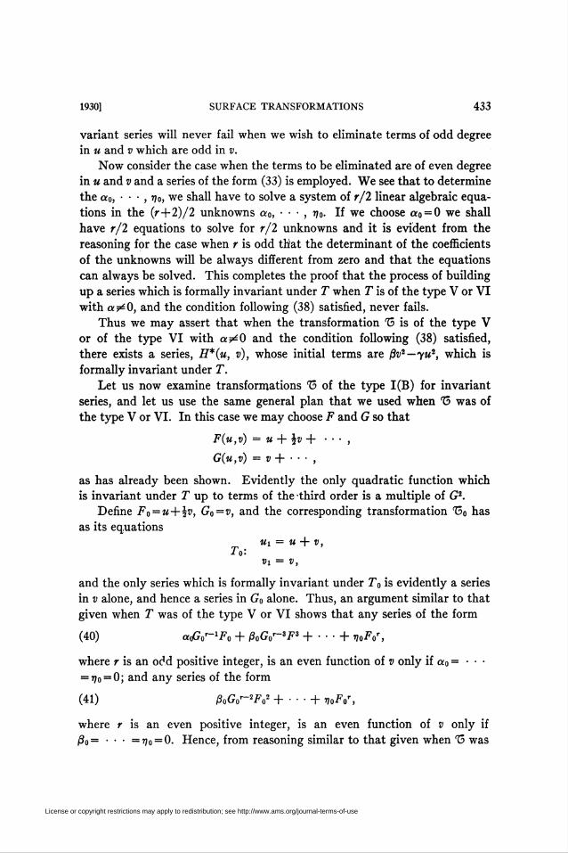
Let us now examine transformations 15 of the type 1(B) for invariant
series, and let us use the same general plan that we used when 15 was of
the type V or VI. In this case we may choose F and G so that
F(u,v) = M + %v+ ■ ■ ■ ,
G(u,v) = v+ ■ ■ ■ ,
as has already been shown. Evidently the only quadratic function which
is invariant under T up to terms of the third order is a multiple of G2.
Define F0 = u+%v, G0=v, and the corresponding transformation 150 has
as its equations
Mi = m + v,T0:
Vx = V,
and the only series which is formally invariant under T0 is evidently a series
in v alone, and hence a series in G0 alone. Thus, an argument similar to that
given when T was of the type V or VI shows that any series of the form
(40) aoGo'-^o + ßoG0'-*F3 +■■■+ r,0F0r,
where r is an odd positive integer, is an even function of v only if a0 = ■ ■ ■
= 770 = 0; and any series of the form
(41) ßoG0r-2Fo2 + ■ ■■ + T)oFor,
where r is an even positive integer, is an even function of v only if
ßo= • ■ ■ =t?o = 0. Hence, from reasoning similar to that given when 15 was
License or copyright restrictions may apply to redistribution; see http://www.ams.org/journal-terms-of-use

434 F. R. BAMFORTH [July
of the type V or VI, it follows that every transformation of the type 1(B)
possesses a formally invariant series whose initial term is v2.
Let us now consider transformations of the type 11(B). The only series
invariant under the corresponding Ta are series in — u, i.e., Go. Thus it is
evident, from the type of reasoning given above, that for any transformation
of this type there exists an invariant series whose first and second degree
terms are all zero except the one involving m2, which is not zero.
Now consider the possibility of invariant series for the cases where 13
can be represented by equations of the form 1(A), 11(A), III or IV. Since
series invariant under the corresponding equations T0 may be series in F0
only, we see that our method of proving the existence of invariant series fails
since a series of the form (40) or (41) may be an even function of v and still
not have a0= ■ ■ ■ =tj0 = 0. However, on making use of the fact that our
method does fail, we can actually set up transformations of these types which
possess no formally invariant series. This is due to the fact that, for these
cases, the determinant of the coefficients in the equations which determine
the cto, • • ■ , vo of (33) and (34) may now be zero, and by a proper choice of
the coefficients of the F and the G these equations will be inconsistent. Hence
we can only say that transformations of the types 1(A), 11(A), III and IV
may or may not have formal invariant series.
We may say by way of summary that for equations T of the types 1(B),
11(B), V and VI (ot^O, and 6 satisfying the condition mentioned after (38)),
there always exist formal invariant series; but for equations of the other types
such series need not exist.
V. Totality of invariant series
For certain types of transformations 13 we have proved the existence of
formal invariant series and have given rules for finding particular ones. We
now wish to prove that for any given transformation every formal invariant
series is a formal series in powers of a particular one.
Let us first consider those transformations of types V and VI for which
we proved the existence of invariant series. As we have seen, there is no
invariant series with any terms of degree less than two. Hence, in every
invariant series, the terms of lowest degree are of at least the second degree.
Now suppose that the degree of the lowest degree terms of a formal invariant
series is r = 2, and suppose that these terms do not form a multiple of some
power of
bioboiFo2 — aoiflioGo2
of (32). Since the invariancy of these terms is due entirely to their properties
License or copyright restrictions may apply to redistribution; see http://www.ams.org/journal-terms-of-use
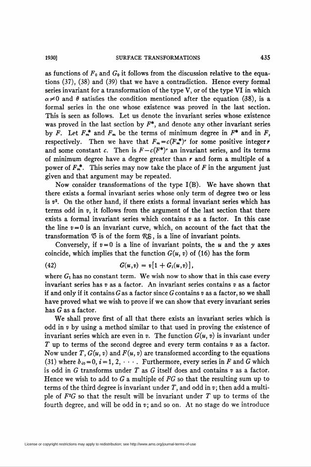
1930] SURFACE TRANSFORMATIONS 435
as functions of F0 and G0 it follows from the discussion relative to the equa-
tions (37), (38) and (39) that we have a contradiction. Hence every formal
series invariant for a transformation of the type V, or of the type VI in which
a^O and 6 satisfies the condition mentioned after the equation (38), is a
formal series in the one whose existence was proved in the last section.
This is seen as follows. Let us denote the invariant series whose existence
was proved in the last section by F*, and denote any other invariant series
by F. Let F* and Fm be the terms of minimum degree in F* and in F,
respectively. Then we have that Fm = c(P*)r for some positive integer r
and some constant c. Then is F—c(F*)T an invariant series, and its terms
of minimum degree have a degree greater than r and form a multiple of a
power of Fm. This series may now take the place of F in the argument just
given and that argument may be repeated.
Now consider transformations of the type 1(B). We have shown that
there exists a formal invariant series whose only term of degree two or less
is v2. On the other hand, if there exists a formal invariant series which has
terms odd in v, it follows from the argument of the last section that there
exists a formal invariant series which contains v as a factor. In this case
the line v = 0 is an invariant curve, which, on account of the fact that the
transformation 15 is of the form îfê, is a line of invariant points.
Conversely, if v = 0 is a line of invariant points, the u and the y axes
coincide, which implies that the function G(u, v) of (16) has the form
(42) G(u,v) = v[l+Gx(u,v)],
where Gx has no constant term. We wish now to show that in this case every
invariant series has sasa factor. An invariant series contains nasa factor
if and only if it contains G as a factor since G contains v as a factor, so we shall
have proved what we wish to prove if we can show that every invariant series
has G as a factor.
We shall prove first of all that there exists an invariant series which is
odd in v by using a method similar to that used in proving the existence of
invariant series which are even in v. The function G(u, v) is invariant under
T up to terms of the second degree and every term contains v as a factor.
Now under T, G(u, v) and F(u, v) are transformed according to the equations
(31) where bi0 = 0, i = 1, 2, • • • . Furthermore, every series in F and G which
is odd in G transforms under Z1 as G itself does and contains sas a factor.
Hence we wish to add to G a multiple of FG so that the resulting sum up to
terms of the third degree is invariant under T, and odd in v; then add a multi-
ple of F2G so that the result will be invariant under T up to terms of the
fourth degree, and will be odd in v; and so on. At no stage do we introduce
License or copyright restrictions may apply to redistribution; see http://www.ams.org/journal-terms-of-use
436 F. R. BAMFORTH [July
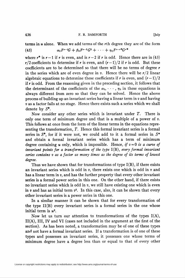
terms in u alone. When we add terms of the rth degree they are of the form
(43) aoF'-'G + ß0F^G3 + • • • + rnF"*G'*
where r* is r — 1 if r is even, and is r — 2 if r is odd. Hence there are in (43)
r/2 coefficients to determine if r is even, and (r —1)/2 if r is odd. But these
coefficients are to be determined so that there will be no terms of degree r
in the series which are of even degree in v. Hence there will be r/2 linear
algebraic equations to determine these coefficients if r is even, and (r —1)/2
if r is odd. From the reasoning given in the preceding section, it follows that
the determinant of the coefficients of the a0, ■ ■ ■ , r¡0 in these equations is
always different from zero so that they can be solved. Hence the above
process of building up an invariant series having a linear term in v and having
v as a factor fails at no stage. Hence there exists such a series which we shall
denote by S*.
Now consider any other series which is invariant under T. There is
only one term of minimum degree and that is a multiple of a power of v.
This follows at once from the form of the linear terms in the equations repre-
senting the transformation, T. Hence this formal invariant series is a formal
series in S*, for if it were not, we could add to it a formal series in S*
and obtain a formal invariant series which has a term of minimum
degree containing u only, which is impossible. Hence, if v = 0 is a curve of
invariant points for a transformation of the type 1(B), every formal invariant
series contains v as a factor as many times as the degree of its terms of lowest
degree.
Thus we have shown that for transformations of type 1(B), if there exists
an invariant series which is odd in v, there exists one which is odd in v and
has a linear term in v, and has the further property that every other invariant
series is a formal power series in this one. On the other hand, if there exists
no invariant series which is odd in v, we still have existing one which is even
in v and has as initial term v2. In this case, also, it can be shown that every
other invariant series is a power series in this one.
In a similar manner it can be shown that for every transformation of
the type 11(B) every invariant series is a formal series in the one whose
initial term is u2.
Now let us turn our attention to transformations of the types 1(A),
11(A), III, IV and VI (cases not included in the argument at the first of the
section). As has been noted, a transformation may be of one of these types
and not have a formal invariant series. If a transformation is of one of these
types and possesses an invariant series, it possesses one whose terms of
minimum degree have a degree less than or equal to that of every other
License or copyright restrictions may apply to redistribution; see http://www.ams.org/journal-terms-of-use

1930] SURFACE TRANSFORMATIONS 437
invariant series. Then it can be proved by means of methods other than those
used above that every formal invariant series is a formal series in one such
as has just been described.f
VI. Invariant curves
Let us fix our attention on any particular transformation T3 =5^S, and
consider any curve C which passes through the origin. It is reflected by S
in the y axis into a curve C, and C, is reflected by íR. in the u axis into a curve
Cm = Ct. If the curve C is invariant under 15, it is the same as Ct. But C*
and C, are, in the uv system of coordinates, the reflection images of one
another in the u axis. Hence, if C = C<, we see that C and C, are the reflection
images of one another in the u axis in the uv system of coordinates as well as
the reflection images of one another in the yx system of coordinates. Hence,
if C is invariant under 15, C, is also, and thus we see that invariant curves
occur in pairs, each curve of every pair being the reflection of the other curve
of the same pair in the y axis under S and in the u axis under %. We shall
call such a pair of invariant curves a "pair of conjugate curves." It may
happen, of course, that a pair of conjugate invariant curves consists of only
one curve counted twice.
Let us now discuss the possibility of there being curves of invariant points
through the origin. If such curves exist, it follows from the equations (24)
for the transformation 15 that the coordinates of their points must satisfy
the equations
F(u, - v) = F(u,v), G(u-, - v) = -G(u,v),
which implies that such curves are analytic. The above equations also show
that either the origin is an isolated invariant point or there exists a curve
of invariant points passing through it.
It is of interest to note that if the points on an invariant curve through
the origin are not invariant, they either approach the origin under the trans-
formation 13 or recede from it. If the points on one invariant curve approach
the origin under the transformation, the points on its conjugate recede from
the origin. But a proof of this latter fact will be omitted since it is not used
in any of the discussion to follow.
We now wish to discuss the relationships existing among formal invariant
series, formal invariant curves through the origin, and actual invariant
curves through the origin. In case there exists a formal invariant series,f
j B, p. 25. Reference is to the first part of the theorem only. To prove our statements are
correct for transformations of the types 11(A) and IV, note that every series formally invariant under
T is also invariant under T2.
X B, pp.18-33.
License or copyright restrictions may apply to redistribution; see http://www.ams.org/journal-terms-of-use
438 F. R. BAMFORTH [July
F(u, v), then every real formal curve which makes a factor of this series
vanish is a formal invariant curve, and conversely, every formal invariant
curve which is not made up of invariant points makes one of the factors of
F vanish. That a formal invariant curve consisting of invariant points does
not necessarily make a factor of F vanish will be shown to be the case by
means of an example in the next section. It will be shown in this same section
that there may exist formal invariant curves and yet no invariant series.
This illustrates some of the radical differences between transformations of
the type discussed in this paper and those of the type discussed by Birkhoff,
for when a transformation is represented by equations whose linear terms are
those of the type 1(A), it possesses an invariant series if it is conservative,
and every formal invariant curve, whether made up of invariant points
or not, makes one of the factors of this series vanish.
It has been shown,f in an ingenious manner, that to every real formal
invariant curve of a conservative transformation of any one of a number
of types there corresponds one and only one actual invariant curve, which,
moreover, is hypercontinuous at the origin which is the invariant point
under consideration, and has the formal invariant curve as its asymptotic
representation.
Furthermore, in any sector of a neighborhood of the origin, sufficiently
small, which does not contain any invariant curve which has a formal in-
variant curve as its asymptotic representation at the origin, and which is
bounded by two such invariant curves which are not curves of invariant
points, no point remains on indefinite iteration of the transformation or of
its inverse.
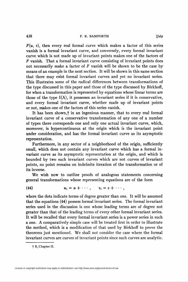
We wish now to outline proofs of analogous statements concerning
general transformations whose representing equations are of the form
(44) Mi = m + • • • , Vi = v + • • • ,
where the dots indicate terms of degree greater than one. It will be assumed
that the equations (44) possess formal invariant series. The formal invariant
series used in the discussion is one whose leading terms are of degree not
greater than that of the leading terms of every other formal invariant series.
It will be recalled that every formal invariant series is a power series in such
a one. A comparatively simple case will be treated first in order to illustrate
the method, which is a modification of that used by Birkhoff to prove the
theorems just mentioned. We shall not consider the case where the formal
invariant curves are curves of invariant points since such curves are analytic.
f B, Chapter II.
License or copyright restrictions may apply to redistribution; see http://www.ams.org/journal-terms-of-use

1930] SURFACE TRANSFORMATIONS 439
We shall suppose that the real formal invariant curve under consideration
is regular at the origin, i.e., can be represented in the form w = a power series
in v, or in the form v = a power series in u. Let us suppose that our curve is
given in the latter form and that its equation is
(45) v = p(u) = axu + a2u2 + ■ • • .
If we perform the formal change of coordinates
(46) m* = m, v* = v — p(u),
the formal curve (45) is taken as the u* axis and the equations of the trans-
formation are reduced to the form
(47) * •/, .i \»i* = v*(l + ■ • •),
and the transform of the formal invariant series used has v* as a factor, i.e.,
(48) F(«,tO~»*(---).
In the series on the right hand side of the first equation of (47) let au*p be
the first term, other than u*, which does not contain v* as a factor. There is
such a term, for otherwise v* = 0 is a formal curve of invariant points which is
contrary to supposition. For definiteness in argument we shall suppose
thata>0.
There are two distinct cases to consider, the first being where the formal
invariant series of (48) in u* and v* contains a term containing u*, and the
other the case where the formal invariant series contains no such term. We
shall now consider the first case.
Let the equations f which represent the ktW iterate of this transformation
be
«* = £ <t>mnU*mV*n,
and define
m+B—1
on
m+n=l
v* = X) 4>Zu*mv*n
du*(49) ou* = —
ok
, * dv*, ôv* =-
*-o àk t=o
whence Su* and Sv* are formal series in u* and v*. Now the formal series F
satisfies the equation
tB.p.10.
License or copyright restrictions may apply to redistribution; see http://www.ams.org/journal-terms-of-use
440 F. R. BAMFORTH [July
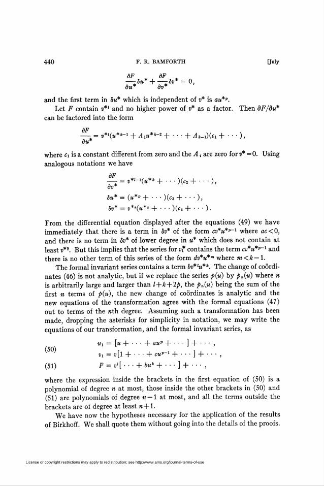
dF dF— 8u* + —ôv* = 0,du* dv*
and the first term in ou* which is independent of v* is au*p.
Let F contain v*1 and no higher power of v* as a factor. Then dF/du*
can be factored into the form
dF„*/(„**-! + AlU*k-2 + ... + Ak_i)(ci +•••),
du*
where Ci is a constant different from zero and the A < are zero for v* = 0. Using
analogous notations we have
^- = „*<-i(„**+...)(Cs+...),dv
8u*=*(u**+■ ■•)(€,+ ■•■),
ÔV* = v*'(u*° + • • -)(C4+ • • •)•
From the differential equation displayed after the equations (49) we have
immediately that there is a term in 8v* of the form cv*u*p~l where ac<0,
and there is no term in 8v* of lower degree in u* which does not contain at
least v*2. But this implies that the series for v* contains the term cv*u*p~l and
there is no other term of this series of the form dv*u*m where m<k — 1.
The formal invariant series contains a term bv*lu*k. The change of coordi-
nates (46) is not analytic, but if we replace the series p(u) by pn(u) where n
is arbitrarily large and larger than l+k+2p, the pn(u) being the sum of the
first n terms of p(u), the new change of coordinates is analytic and the
new equations of the transformation agree with the formal equations (47)
out to terms of the nth. degree. Assuming such a transformation has been
made, dropping the asterisks for simplicity in notation, we may write the
equations of our transformation, and the formal invariant series, as
Mi = [u + • • • + aup +•••] + ••• ,
vi = v[l + • • • + cup~l+ •••] + •••,
F = vl[--- + bu"+ ■■■] + ■■■ ,
where the expression inside the brackets in the first equation of (50) is a
polynomial of degree n at most, those inside the other brackets in (50) and
(51) are polynomials of degree n — 1 at most, and all the terms outside the
brackets are of degree at least w+1.
We have now the hypotheses necessary for the application of the results
of Birkhoff. We shall quote them without going into the details of the proofs.
(50)
(51)
License or copyright restrictions may apply to redistribution; see http://www.ams.org/journal-terms-of-use
1930] SURFACE TRANSFORMATIONS 441
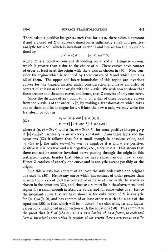
There exists a positive integer n0 such that for n>n0 there exists a constant
d and a closed set 2 of curves defined for u sufficiently small and positive,
analytic for u > 0, which is invariant under 13 and lies within the region de-
fined by0 < m < d, \v | < £»"-»•,
where E is a positive constant depending on n and d. Define ?» = »—n0,
which is greater than p due to the choice of n. These curves have contact
of order at least m at the origin with the u axis as chosen in (50). Now con-
sider the region which is bounded by these curves of 2 and which contains
all of them. The upper and lower boundaries of this region are invariant
curves for the transformation under consideration and have an order of
contact of at least m at the origin with the u axis. We wish now to show that
these are one and the same curve, and hence, that 2 consists of only one curve.
Since the distance of any point (u, v) on either of these boundary curves
from the u axis is of the order \u \m, by making a transformation which takes
one of them and its analogue for u < 0 into the new u axis, we may write the
transform of (50) as
«i = [« + aup] + (j>x(u,v),
vx = v{ [l + cm"-1] + <t>2(u,v)},
where <px(u, v) =0(uq) and <f>2(u, v) =0(uq~l), for some positive integer q>p
if \v | <c0 \u" \, where c0 is an arbitrary constant. From these facts and the
equations (52) it follows that for u small enough in absolute value, and
|u| <£o|wp|, the ratio (vx—v)/(ux—u) is negative if u and v are positive,
positive if m is positive and v is negative, etc., since ac<0. This show's that
there can not be another invariant curve passing through the origin in this
restricted region, besides that which we have chosen as our new u axis.
Hence 2 consists of exactly one curve and is analytic except possibly at the
origin.
But this u axis has contact of at least the wth order with the original
one used in (50). Hence any curve which has contact of order greater than
m with the u axis of (50) has contact of order m at least with the u axis as
chosen in the equations (52), and, since m >p, must lie in the above mentioned
region for u small enough in absolute value, and for some value of c. Hence
the invariant curve that we have shown is the only curve of S, is analytic
for (u, v)y^(0, 0), and has contact of at least order m with the u axis of the
equations (50), is that which will be obtained if we choose higher and higher
values for n mentioned in connection with the equations (50). This completes
the proof that if F of (48) contains a term having u* as a factor, to each real
formal invariant curve which is regular at the origin there corresponds exactly
License or copyright restrictions may apply to redistribution; see http://www.ams.org/journal-terms-of-use
442 F. R. BAMFORTH [July
one actual invariant curve which has this formal invariant curve as its asymp-
totic representation at the origin.
Let us now consider what can be said about the series for Vi in case the
formal invariant series F in (48) contains no term in u*. In this case there is
only one real formal invariant curve which is not a curve of invariant
points, and when that has been transformed formally into the u* axis the
expression for v* is a power series in v* alone. But if the series F has no term
involving u* its term of minimum degree is a multiple of a power of v*,
and, since the degree of this term is not greater than that of the corresponding
term in every other formal invariant series, it is one. But if there is a formal
invariant series whose leading term is v* which contains no term involving u*,
there is one whose only term is v*. Hence there is a formal invariant series
for the transformation represented by the equations (44) of the form v—p(u)
where p(u) is a power series in u.
Let us now recall that we intend to apply the discussion of this section
to transformations of the type 13 =<R£ where ^ and S are each of the reflec-
tion type, and we shall assume that the coordinate system used is a normal
one for the transformation %,. Under these assumptions, if there exists a
formal invariant series of the form v — p(u) there exists one of the form
v-\-p(u) which is implied by the discussion of Section IV, and this implies
that v is an invariant function which, in turn, implies that the second equation
of (44) has the form Vi = v. In this case v = 0 is an invariant curve. Hence,
when a transformation 13=^5 is represented by equations of the form (44)
where the uv system of coordinates is normal for <î\, and if there is a formal
invariant series for this transformation which can be formally reduced to a
formal series in v* alone by means of a change of variables of the form (46), v = 0
is an invariant curve and, on account of the fundamental properties of 13 as
the product of % and S , it follows that v = 0 is a curve of invariant points.
Now let us consider the transformations whose representative equations
have the form (44) but whose formal invariant curves have "cusps" at the
origin. By use of transformations of the type
(53) « = u*v*, v = v*,
such formal invariant curves are taken into ones of the first type considered
in the above argument, i.e., the reduced equations representing the trans-
formation have not a formal invariant series of the form v*—p(u*). This is
due to the fact that on account of the nature of the change of variables (53)
there is one formal invariant series F* which contains either u* or v* as a
factor, and to the fact that, according to Section V, every other formal in-
variant series is either a root or a formal power series in F*.
License or copyright restrictions may apply to redistribution; see http://www.ams.org/journal-terms-of-use
1930] SURFACE TRANSFORMATIONS 443
Hence, if there exists a real, formal, invariant series, to every real formal
invariant "cusp," there corresponds one and but one real invariant curve which
has this formal invariant curve as its asymptotic representation.
Finally, concerning the stability of the invariant point (u, v) = (0, 0)
under a transformation represented by equations of the form (44), it may
be said that in case a formal invariant series exists, in any sector of a suffi-
ciently small neighborhood of the origin, which does not contain any invariant
curve which has a formal invariant curve as its asymptotic representation at the
origin, and which is bounded by two such invariant curves which are not curves
of invariant points, no point remains on indefinite iteration of the transformation
or of its inverse. The proof of this statement is omitted here since it is almost
exactly that given in the discussion of conservative transformations which
has been mentioned before.
VII. Transformations of type 1(A)
One of the chief differences between conservative transformations and
those of the type studied in this paper is that for conservative transforma-
tionsf of type II", which correspond to transformations of the type 1(A),
there always exist real formal invariant series, while such series need not exist
for transformations of the type 1(A). Due partially to the fact that formal
invariant series need not exist, a wide variety of situations occur which are
interesting in comparison with the facts known concerning conservative
transformations of the type II". These situations will now be studied in
some detail, while the analogous ones which arise for the other types of trans-
formations for which there may not be any formal invariant series will
hardly be mentioned since the discussion for type 1(A) will be typical of
that which could be given for them too.
We shall confine our attention to a neighborhood of the origin of coordi-
nates which is supposed to be an invariant point. Questions which have to
be answered are those relative to the existence of invariant curves through
the origin, existence of invariant integrals, existence of invariant series, and
stability.Let us first note that in Section III we have already shown that all
directions through the origin are invariant under a transformation of the
type 1(A). We shall now show that for transformations of type 1(A), (i)
the existence of a formal invariant integral implies the existence of a formal in-
variant series; (ii) the existence of a formal invariant series- does not imply
the existence of a formal invariant integral ; (iii) the existence of invariant curves
does not imply the existence of formal invariant series; and (iv) the existence
t See last of Section II.
License or copyright restrictions may apply to redistribution; see http://www.ams.org/journal-terms-of-use

444 F. R. BAMFORTH [July
of formal invariant series which possess real factors] implies the existence of
real invariant curves through the origin. The proof of (i) is already in the
literature.t
We shall prove (ii) by means of an example. Consider the transformation
defined by the following equations:
1 - vMi = M, Mi = M-,
1 + VR: S:
vi = - v; vi= - v;(54)
1 — vMi = M-)
T = RSi l + v
Vi = V.
Each of the transformations defined by the equations R and S is of the
reflection type and it is evident that any series in v is formally invariant
under T. We need only show that there exists no quasi-invariant series.
Evidentlyd(Ui,Vi) _ 1 — v
d(u,v) 1 + v
Now if Q(u, v) is a quasi-invariant series we have
d(«i,*i)Q(u,v) = Q(ui,vi)-->
d(u,v)
and we must remember that Q(Q, 0) is different from zero. Let
Q(u,v) = çoo + gio« + qoiv + • • • .
Then
0(u,.v,)d(u,v)
d(ui,Vi) /l — v\Q(ui,vi) —-— = (qoo + qioUi + qoiVi +•••)(-)
\1 + v/
= Coo + gioM + (g0i — 2qoo)v + • • • .
Since g0o ̂0, this equation shows that no formal quasi-invariant series Q
can exist for the transformation represented by (54).
We shall now show by an example that a transformation of the type 1(A)
may possess an invariant curve through the origin and yet possess no formal
invariant series. Consider the transformation for which the equations (16) are
(55) y = M + »3, x = v + m3.
tB,P.18.t B, p. 16. In this paper, the assumption is made that the transformation possess an actual
invariant integral, but for the proof tof (i) no use is made of the fact that the quasi-invariant series Q
is convergent.
License or copyright restrictions may apply to redistribution; see http://www.ams.org/journal-terms-of-use

1930] SURFACE TRANSFORMATIONS 445
Evidently
X1 — Jl2 = (v2 — M2)(l — 2UV — V* — V2U2 — M4).
Hence a;2—y2 = 0 is equivalent to v2—u2 = 0. But the curves a;2—y2 = 0 are
the images of one another under S and the same curves v2—w2 = 0 are the
images of one another under % Hence the curves x2—y2 = 0, which are the
same as the curves v2—m2 = 0, are a pair of conjugate invariant curves
through the origin for the transformation 13 =<R.S.
Now turn to the equations (55) and investigate the possibility of the
existence of a formal invariant series. We have seen that if such a series
exists at all, there exists one that is even in v+u3 and which, when expanded
in terms of u and v, is even in v. Furthermore, if there exists such a series,
there exists one whose lowest degree terms are of even degree in (v+u3)
and (u+v3). Let the lowest degree terms of such a series be
(56) ar(v + u3Y + ar-2(v + u3)r~2(u + v3)2 -\-\- a0(u + v3)*,
where r is an even positive integer. In this series (56) there exists no term of
degree r+l in u and v. Furthermore, in our invariant series, when the terms
of degree r+1 in (v+u3) and (u+v3) are expanded, there will be no terms of
degree r+2. Hence the terms of (56) which are of degree r+2 in u and v
but odd in v have to be counterbalanced as in Section IV, by the addition
of a sum of the form
(57) bo(v + u3Y+2 + b2(v + u3Y(u + v3)2 -\-+ br+2(u + v3)*2.
But there exist no terms in this series of degree r+2 which are of odd degree
in v, and since the terms of (56) of degree r+2 which are of odd degree in
v are
rart)r_1M3
+ 2ar~2v'-lu + (r — 2)ar-2vr~3ub
+ 4ar_4Dr~1M3 + (r — 4)ar_4í),_6M7
+ 6ffr-«î>r-3M6 + • • •
it is evident that ar_2 = ar_6 = ar-io= • • • =0 and rar+4ar_4 = 0, (r—4)ar_4
+8ar_8 = 0, • • • . But since ar_4a = 0 where 4a is the largest multiple of 4
which is not greater than r, we see that each of this last set of a< is also zero,
and hence there can exist no invariant series, although there exist analytic
invariant curves through the origin.
License or copyright restrictions may apply to redistribution; see http://www.ams.org/journal-terms-of-use

446 F. R. BAMFORTH [July
In connection with transformations of the type 1(A) it is of interest to
know when there are curves of invariant points through the origin. Let the
equations (16) be denoted by
y = « + /(«,»), x = v + g(u,v),
where/ and g are convergent series in u and v which have no terms of degree
less than two. Then the transformation 13 is represented by the equations
mi +/(«i, - vi) = m + /(m,d),
- »i + g(ui, - vi) = - v - g(u,v).
The points that are invariant under 13 are given by
« + /(«, - v) = M + f(u,v), - v + g(u, - v) = - v - g(u,v),
\.e.,f(u,—v) =f(u, v), g(u,—v) = —g(u, v). This means that/is an even func-
tion of v and g is an odd function of v for (u, v) an invariant point. Hence,
if/ and g are such that for curves passing through the origin these equations
are satisfied, these curves are curves of invariant points.
We have given examples of transformations under which certain curves
passing through the origin are invariant. On the other hand, there exist
transformations of the type 1(A) under which no curve through the origin
is invariant. An example of such a one is the transformation for which the
equations (16) are
y = M + ï3, x = v — m',
but we shall not pause to prove this fact.
In the study of conservative transformations the fact was discovered
that, for each transformation of type II", every invariant curve that passes
through the origin and is hypercontinuous there has an asymptotic expansion
at the origin which formally makes every formal invariant series zero, and
formal invariant series always exist. We have already shown that for the
analogous transformations of type 1(A) there may exist analytic invariant
curves through the origin and yet no formal invariant series; now we shall
give an example of a transformation of type 1(A) which has an invariant
series and an analytic invariant curve through the origin along which the
series is not formally zero. This invariant curve is necessarily a curve of
invariant points.f
Consider again the transformation represented by
«i = m(1 — i»)/(l + v), Vi = v.
tB, pp. 31-32.
License or copyright restrictions may apply to redistribution; see http://www.ams.org/journal-terms-of-use

1930] SURFACE TRANSFORMATIONS 447
Any formal series in v is a formal invariant series. Yet « = 0 is a line of in-
variant points and u is not a factor of any formal invariant series.
Finally, in connection with the questions relative to actual invariant
curves corresponding to real factors of a formal invariant series, and questions
of stability, we shall merely draw attention to the fact that the discussion
of Section VI is applicable in this one.
VIII. Transformations of type 1(B)
We have already shown that for such transformations there always
exists a formal invariant series which is even in v, whose only term of degree
less than three is v2. Hence this formal invariant series can be factored in
the form(v2 + f(u))(l + ■ ■ ■ )
where f(u) is a formal series in u whose term of lowest degree we shall denote
by aup in case f(u) is not identically zero. As has already been seen in Sec-
tion IV, f(u) is identically zero if and only if v = 0 is a line of invariant points.
On the other hand, \îf(u) is not identically zero, v2+f(u)=0 represents
a real, formal, invariant curve with a "cusp" at the origin if p is odd, and
two real, formal, invariant curves tangent at the origin if a<0 and p is even.
If a>0 and p is even, there is no real, formal, invariant curve through the
origin.
A change of coordinates of the type u = u*, v=u*v* reduces the equations
representing a transformation of the type 1(B) to equations of the type (44),
and hence the methods of Section VI show that, when there is a formal invari-
ant "cusp," there is a unique actual invariant curve having this formal "cusp"
as its asymptotic representation at the origin, and when there are two real
formal invariant curves through the origin there are exactly two actual
invariant curves tangent to the u axis at the origin and having these formal
curves as their asymptotic representations.
Furthermore, when invariant curves through the origin exist, the origin
is an unstable hyperbolic point, and the argument at the end of Section VI
shows that if a sufficiently small neighborhood of the origin be chosen, points
not on the invariant curves in this neighborhood do not remain in it on
iteration of the transformation or of its inverse.
With transformations of the type 1(B) there are connected formal differ-
ential equations of the type (49) which were used in the discussion of equa-
tions of the type (44). But for such a transformation the highest common
factor of 8u and 8v is v, and there is a curve of invariant points only if there
exists an invariant series having v2 as a factor. Hence, f transformations of
the type 1(B) are formally conservative.
t B, p. 19 et seq.
License or copyright restrictions may apply to redistribution; see http://www.ams.org/journal-terms-of-use
448 F. R. BAMFORTH [July
IX. Transformations of types 11(A) • • • IV
For all these transformations, except those of type 11(B), there may or
may not exist formal invariant series. For transformations of the type II (B),
a discussion analogous to that given for transformations of type 1(B) can
be given. It may be noted, however, that in this case there can be no curve
of invariant points through the origin. There may, however, exist a curve
through the origin which is invariant under the transformation and which
consists of points all of which are invariant under 132.
As has already been mentioned, a discussion similar to that given for
transformations of the type 1(A) may be given here for each of the other
transformations named in this section. This we shall not do, but shall con-
tent ourselves with merely pointing out a few of the main distinctions.
For transformations of the type 11(A) the origin is an isolated invariant
point, and the points on every invariant curve through the origin transform
under 13 into points, each of which is separated on the invariant curve
from its image by the origin. This is a direct consequence of the form of the
linear terms in the equations for T in (25). The discussion of Section VI
is evidently applicable to the second iterate of a transformation of the
type 11(A).If a transformation is of the type III, the origin is an isolated invariant
point unless there is a single curve of invariant points through it. This is
shown as follows. Let the equations (16) be denoted by
y = M+/(M,»), x = \u + v + g(u,v),
where all the terms of / and g are of degree higher than two. The invariant
points are given by
/(«, - v) = f(u,v), - m = g(u, - v) + g(u,v).
The form of these equations at once proves that the statement above is
correct.
The origin, for transformations represented by equations of the types
11(B), III and IV of (25), is an unstable invariant point, and may be either
hyperbolic or elliptic.
X. Transformations of type V
If a transformation is of type V, by means of a real linear change of vari-
ables, equations representing it may be chosen which have the form
(58) Mi = pu + • • ■ , vi= (1/p) v+ ■ ■ ■ , p = a±(a2- l)W * 0,
where now the uv system of coordinates is not normal for %_. Any transforma-
tion represented by equations of this form in which the right hand members
License or copyright restrictions may apply to redistribution; see http://www.ams.org/journal-terms-of-use
1930] SURFACE TRANSFORMATIONS 449
are analytic possessesf two real analytic invariant curves through the origin
whose equations may be written in the form u=f(v), v=g(u). When these
curves are taken as axes, it can be readily shown that the points on one of
these curves in a neighborhood of the origin move into the origin on iteration
of the transformation, while the points on the other curve move away from
the origin. In the case where p < 0 the origin always lies between a point and
its image when these points lie on one of the invariant curves through the
origin.} Furthermore, a neighborhood of the origin can be taken so small that
any point in it not on one of these invariant curves through the origin moves
out of it on iteration of the transformation or of its inverse. Hence, trans-
formations of the type V are hyperbolic and unstable.
We now wish to point out the interesting facts that there is a formal
equivalence existing between transformations of the type V and conservative
transformations of the types I' and I". We shall first prove that every
transformation of the type I' or of the type I" is formally of the type V
and hence is formally the product of two transformations each of the reflec-
tion type.§ Now the equations representing a conservative transformation
of the type I' or of the type I", by a formal change of variables, may be given
either the form^f
1(59) Ux = pUefiW1, Vx = — Ve~^1^, c * 0,
P
or the form
(60) Ux = pU, Vx = —V.P
But the equations (59) are the product RS of the two systems
r Ux = pVe'VV, s¡ Ux = V,
'' Vx = ±Ue-<u'V; Vx = U,P
each of which is of the "reflection" type. Evidently the equations (60) are
also the product of two systems each of the "reflection" type.
We shall now prove that, conversely, the equations representing a trans-
formation of type V are, by a formal change of variables, equivalent to equa-
tions of the form (59) or (60), and that every transformation of type V is
t Poincaré, Œuvres, vol. I, p. 202.
j Cf. Section III.
§ This fact was kindly pointed out to the author by Professor Birkhoff.
UB, pp. 34,55.
License or copyright restrictions may apply to redistribution; see http://www.ams.org/journal-terms-of-use
450 F. R. BAMFORTH
formally conservative. Let us assume that the equations representing the
transformation of type V under consideration are in the form (58). From
our previous discussion we know that there exists a formal invariant series
whose only term of degree less than three is cuv where c is a constant different
from zero. When p>0, we know that there existsf a formal quasi-invariant
series and hence that our transformation is formally conservative and that
its representative equations may be formally reduced to the form (59) or
to the form (60). When p<0, the equations for 132 are of the same form as
(58) with p replaced by p2, and hence represent a formal conservative trans-
formation. Hence they can be reduced to the form (59) or to the form (60)
and hencej the transformed equations of 15 have the same form.
XL Transformations of type VI
Transformations of type VI where p satisfies the condition mentioned
after the equations (38) are formally conservative, and transformations
which are conservative and of the type II' are formally the product of two
transformations each of the reflection type. We shall not give proofs of these
statements since they are wholly similar to those of the analogous statements
made in the previous section.
On account of the form of the initial terms in the invariant series which we
proved to exist for transformations of this, type, it is evident that no formal
invariant curves exist through the origin. In fact, the discussion given in
Section III shows that there can exist no invariant curve of any kind through
the origin since no slope through the origin is invariant. Hence the origin is
an elliptic invariant point which raises many important and interesting ques-
tions. It will have been observed that the questions answered in the latter
part of this paper have been, to a great extent, concerned with hyperbolic
invariant points. The author hopes to study the elliptic cases in the near
future.
fB, pp. 19-20.ÎB,p.5S.
Cornell University,
Ithaca, N. Y.
License or copyright restrictions may apply to redistribution; see http://www.ams.org/journal-terms-of-use