Embed Size (px)
Citation preview

Loughborough UniversityInstitutional Repository
Surface specific asperitymodel for prediction offriction in boundary and
mixed regimes of lubrication
This item was submitted to Loughborough University's Institutional Repositoryby the/an author.
Citation: LEIGHTON, M. ...et al., 2017. Surface specific asperity model forprediction of friction in boundary and mixed regimes of lubrication. Meccanica,52 (1), pp. 21-33.
Additional Information:
• This is an Open Access Article. It is published by Springerunder the Creative Commons Attribution 4.0 Unported Li-cence (CC BY). Full details of this licence are available at:http://creativecommons.org/licenses/by/4.0/
Metadata Record: https://dspace.lboro.ac.uk/2134/20745
Version: Published
Publisher: c© The Authors. Published by Springer.
Rights: This work is made available according to the conditions of the CreativeCommons Attribution 4.0 International (CC BY 4.0) licence. Full details of thislicence are available at: http://creativecommons.org/licenses/ by/4.0/
Please cite the published version.
Surface specific asperity model for prediction of frictionin boundary and mixed regimes of lubrication
M. Leighton . N. Morris . R. Rahmani .
H. Rahnejat
Received: 27 July 2015 / Accepted: 18 February 2016
� The Author(s) 2016. This article is published with open access at Springerlink.com
Abstract Machine downsizing, increased loading
and better sealing performance have progressively led
to thinner lubricant films and an increased chance of
direct surface interaction. Consequently, mixed and
boundary regimes of lubrication are prevalent with
ubiquitous asperity interactions, leading to increased
parasitic losses and poor energy inefficiency. Surface
topography has become an important consideration as
it influences the prevailing regime of lubrication. As a
result a plethora of machining processes and surface
finishing techniques have emerged. The stochastic
nature of the resulting topography determines the
separation at which asperity interactions are initiated
and ultimately affect the conjunctional load carrying
capacity and operational efficiency. The paper pre-
sents a procedure for modelling of asperity interac-
tions of real rough surfaces, from measured data,
which do not conform to the usually assumed Gaus-
sian distributions. The model is validated experimen-
tally using a bench top reciprocating sliding test rig.
The method demonstrates accurate determination of
the onset of mixed regime of lubrication. In this
manner, realistic predictions are made for load carry-
ing and frictional performance in real applications
where commonly used Gaussian distributions can lead
to anomalous predictions.
Keywords Real rough surfaces � Contact loadcarrying capacity � Friction
List of symbols~A Mean area of asperity contact in the apparent
area of contact
A Apparent area of contact
a Acceleration of floating plate
b Strip face-width
c Lubricant rupture boundary
d Surface separation of mean centrelines
di Height above the centreline of a surface
E0 Composite modulus of elasticity
f Total friction
fb Boundary friction
fv Viscous friction
F5=2 Statistical function for asperity load carrying
capacity
F2 Statistical function for asperity contact area
h Separation or film thickness
h0 Initial gap between surfaces
hini Height of the highest peak relative to the mean
centre-line of the surface
m Mass of floating plate
L Length of sliding strip
p Hydrodynamic pressure
patm Atmospheric pressure
pcav Cavitation pressure
M. Leighton � N. Morris � R. Rahmani (&) � H. RahnejatWolfson School of Mechanical and Manufacturing
Engineering, Loughborough University, Loughborough,
UK
e-mail: [email protected]
123
Meccanica
DOI 10.1007/s11012-016-0397-z

P Load carried by one asperity pair~P Mean asperity load carried for the apparent area
of contact
r Radial distance between asperity tips
R Crown radius of the ring parabolic profile
t Time
U Sliding velocity
w Peak penetration
wp Vertical interference between asperity tips
W Applied load on the strip (total contact load)
Why Hydrodynamic reaction
zi Topography height above the centreline of
surfaces
Z Pressure–viscosity index
Greek symbols
a Piezo-viscosity
b Asperity tip radius
d Surface deformation
g Lubricant dynamic viscosity
g0 Lubricant dynamic viscosity at ambient
conditions
k Stribeck parameter, k = h/rn Asperity density per unit area
q Lubricant density
q0 Lubricant density at ambient conditions
1 Coefficient of the boundary shear strength
/ Probability distribution function
/* Convoluted probability distribution function
r Root mean square variation from mean surface
centreline
s0 Eyring shear stress of the lubricant
W Asperity tip curvatures
1 Introduction
A sufficiently thick low shear strength film of lubricant
is usually desired to form in all contact conjunctions to
carry the applied load and guard against the direct
interaction of asperities on the opposing surfaces, thus
reducing frictional losses. However, in practice this
ideal situation is often not achieved, owing to many
circumstances, such as stop–start or reciprocating
motions, which affect the entrainment of the lubricant
into the contact with relative motion of surfaces [1, 2].
There may also be a lack of lubricant availability at the
inlet to a conjunction as well as reverse and swirl flows
there [3, 4]. As the result, many contacts suffer from a
lack of a coherent lubricant film where a proportion of
applied load is carried by the ubiquitous asperities on
the counterface surfaces. These interactions increase
the generated friction, for example in the cases of
piston-cylinder system at dead centre reversals [5–8]
and cam-follower contact in the inlet reversal posi-
tions [9]. Various palliative actions are undertaken in
order to mitigate these adverse effects within the
mixed regime of lubrication, including the use of hard
wear-resistant coatings. Another approach has been
surface modifications such as cross-hatching of cylin-
der surfaces or texturing in order to entrap reservoirs
of lubricant for instances of poor entraining motion. In
order to opt for any method of palliation, it would be
instructive to initially predict the extent of boundary
interactions in an accurate manner.
Greenwood and Tripp [10] and Greenwood and
Williamson [11] provided mathematical discourses for
asperity interactions between pairs of rough surfaces
for simplified asperity geometry and an assumed
Gaussian distribution of peak heights. A further series
of assumptions were made, most crucially an average
asperity tip radius and an average indentation depth at
given separations with the mutual approach of rough
counterfaces. The method also accounted for the
oblique interaction of any pair of opposing asperities.
These are usually regarded as necessary assumptions
to deal with the complex nature of rough surface
topography. The Gaussian assumption made in Green-
wood and Tripp [10] is not a prerequisite of the
method. Consideration of typical rough surfaces
suggests that a peak height distribution would have a
mean value above the mid-line of the surface as the
majority of the peaks would reside in the upper reaches
of the surface. It is, therefore, advantageous to develop
an asperity model which allows more representative
peak height distributions to be utilised, particularly for
lubricated contacts which were not discussed by
Greenwood and Tripp [10].
Greenwood and Tripp [10] used a Gaussian distri-
bution to approximate the probability of peak height
interactions at a given surface separation; k where thisis inversely proportional to r (root mean square; RMS)
of the surface heights. As a result the mean of the peak
height distribution is set to the same mean as the
surface height distribution as a simplification for the
proof of concept which, for engineering surfaces,
tends to predict that the first surface interactions occur
at a lower value of k than is otherwise the case. This
Meccanica
123

results in an estimate of asperity load carrying capacity
significantly below a real case at the upper reaches of
the surface and a lower separation limit at which the
mixed regime of lubrication is expected to commence.
One way to deal with this shortcoming is to measure
the mean peak height relative to the surface centre-line
and shift the mean of the Gaussian distribution to this
location. This requires the analysis of the surface and
identification of the peak height distribution. There-
fore, ‘‘the surface specific distribution’’ might as well
be used for the rest of the analysis, thus improving the
accuracy of surface representation with little extra
effort. Furthermore, the Gaussian distribution used to
describe the peak height distribution must have the
same standard deviation as the actual peak height
distribution, not the RMS roughness, r, which is
derived from the surface height distribution.
Greenwood and Williamson’s model [11] was
further developed to account for non-uniform radii of
curvature of asperity peaks by Hisakado [12], and for
elliptic paraboloid asperities by Bush et al. [13], as well
as for anisotropic surfaces by McCool [14]. The
Greenwood and Tripp model [10] was extended by
Pullen and Williamson [15] to account for the plastic
deformation of asperities and further improved by
Cheng et al. [16] for an elasto-plastic model. A recent
extension of the model for combined elasto-plastic and
adhesion of asperities for fairly smooth surfaces, using
fractal geometry was reported by Chong et al. [17].
Nevertheless, the original Greenwood and Tripp model
[10] has beenwidely used inmany applications [18–21].
2 Background Theory
It is initially assumed that the surfaces are replaced by
an equivalent surface comprising a collection of
hemispherical asperities of an average tip radius, b
(Fig. 1) and with the same peak height distribution as
the original surfaces themselves.
The asperity radii (b1 and b2) and the radial
separation r allow wp (the peak height interference) to
be related to w (the asperity compression) this results
in the load carrying capacity of the surface. For the
interference of two spheres the asperity compression
can be shown to be:
w ¼ wp �r2
2 b1 þ b2ð Þ
� �ð1Þ
where, hi is a ‘‘Macauley bracket’’. Let:
b ¼ b1 þ b22
ð2Þ
where:
b1 ¼Pn
i¼1 b1in
ð3Þ
The average asperity density over both surfaces
is n and the apparent area of contact is A. Therefore,
the probable load supported by this representative
equivalent surface at a given separation, ~P dð Þbecomes:
~P dð Þ ¼ 2pn2AZr
Zz1
Zz2
P w; rð Þ/ z1ð Þ/ z2ð Þr � dz2�
dz1 � dr ð4Þ
where, P w; rð Þ is the load carried by an asperity pair
with misalignment r and peak penetration of w.
Equation (4) states that the total carried load is as
the result of the load supported at a given penetration
between all pairs of opposing asperities at any given
surface height.
The surface specific contributions are the peak
height distributions, / z1ð Þ and / z2ð Þ, and the asperity
peak density, n. Examples of measured surface height
Fig. 1 Geometry of
asperity pair interaction
Meccanica
123

distributions can be seen in the work of Peklenik [22]
who also discussed some of the key variations between
measured and generated surface properties.
Combining the probabilities by taking the convo-
lution of the asperity peak height distributions for
counterface surfaces leads to:
/� zð Þ ¼ / z1ð Þ � / z2ð Þ ð5Þ
Using Hertzian theory to express the load carrying
capacity as a function of the deformation (penetration)
of two spheres in elastic contact with the effective
composite elastic modulus, E0:
P ¼ 4
3E0W
12w
32 ð6Þ
Where W is the composite curvatures for two
contacting spheres defined as:
1
W¼ 1
b1þ 1
b2ð7Þ
Equation (4) now reduces to:
~P dð Þ ¼ 2pn2AZr
Zz
4
3
� �E0W
12w
32/�ðZÞr:dz:dr ð8Þ
With the inclusion of Eqs. (1) and (2) the equation for
the probable asperity carried load at a given separation
simplifies to:
~P dð Þ¼2pn2AZr
Zz
4
3
� �E0W
12 wp�
r2
4b
� �32
/�ðZÞr:dz:dr
ð9Þ
Extracting the constants and setting the limits of
integration, yields:
~P dð Þ ¼ 8
3pn2E0W
12A
Z 1
d
/� zð Þ � dzZ 1
0
wp �r2
4b
� �32
r � drð10Þ
~P dð Þ ¼ 8
3pn2E0W
12A
Z 1
d
/� zð Þ � dz
� 4
5b wp �
r2
4b
� �52
" #1
0
ð11Þ
~P dð Þ ¼ 32
15pn2E0W
12bA
Z 1
d
z� dh i52/� zð Þ � dz ð12Þ
Standardising the form of the probability distribu-
tion as s ¼ rz:
~P dð Þ ¼ 32
15pn2W
12br
52E0A
Z 1
d=rs� d
r
� �52
/� sð Þ � ds
ð13Þ
Equation (13) can then be rearranged to:
~P dð Þ ¼ 32
15pn2W
12br
52E0AF5
2
d
r
� �ð14Þ
In a similar manner, the mean asperity contact area
within the apparent contact area is found as:
~A dð Þ ¼ 2p2 nrð Þ2WbAF2 kð Þ ð15Þ
Where the probability functions in Eqs. (14) and (15)
are defined as:
Fn kð Þ ¼Z 1
ks� kð Þn/� sð Þ � ds ð16Þ
It is of note that in the original theory proposed by
Greenwood and Tripp [10] the radii on each surface
are assumed to be equal and therefore:
W ¼ b2
ð17Þ
If Eq. (17) is true then Eqs. (14) and (15)
respectively reduce to those given in [10] as
~P dð Þ ¼ 16ffiffiffi2
p
15p nbrð Þ2E0
ffiffiffirb
rAF5
2
d
r
� �ð18Þ
~A dð Þ ¼ p2 nbrð Þ2AF2 kð Þ ð19Þ
The function, F5=2 kð Þ, represents the statistical
likelihood of interactions of deformed asperities at all
separations as one surface is lowered onto the other. In
order to improve the accuracy of the model for a
specific pair of surfaces the specific parameter must be
calculated. The parameters; n, b and r can be readily
determined by many commercially available metrol-
ogy systems. Determination of the function F5=2 kð Þfrom measured surface topography is more involved.
As already noted, to correctly apply the assumption of
a Gaussian distribution of peak heights, the standard
deviation and mean of the peak heights are needed a
priori. However, it is more representative to determine
the peak height distributions of the surfaces through a
simple extension of the approach highlighted above,
using instead the surface specific data.
F5=2 kð Þ and the roughness parameter determine the
probable number of asperities which are penetrated at
Meccanica
123

a given surface separation and the extent of their
deformation.
3 Extension to measured surface data
Measuring surface topography using a variety of
measurement techniques yields an array of surface
height data at discrete measured nodes. The discrete
surface data is then used in a probabilistic model, such
as that described above, with the frequency distribu-
tions required in the form of a histogram of each
surface. The distribution is dependent on the size and
resolution of the sampled area, as well as the surface
itself.
Identifying the asperity summits and their heights
leads to a discrete peak height distribution for each
surface. The convolution of these two peak height
distributions is then found, /�, must conform to:
Z 1
�1/� xð Þ � dx ¼ 1 ð20Þ
Then, the calculation of functions such as F5=2 kð Þ isa routine matter for any desired surface height through
integration of the histogram columns residing above
the k value being considered with a weighting as
shown in Eq. (16).
The remaining surface specific parameters consid-
ered in this model are: n, b, W are and r. The
determination of b and W not considered satisfactory
techniques for measured surfaces. b represents the
mean radius of all the asperity pairs in contact at a
given separation. For multi-scale surfaces, such as
cross-hatched cylinder liners, the manufacturing pro-
cess often comprises several stages. Honing creates a
rough, isotropic surface with a negatively skewed
surface height distribution by machining away the
upper levels of the surface with successively smoother
machining processes. This means that there is a
variation in b at different heights of the surface. At the
upper levels there are likely to be smoother and more
rounded asperities, whilst any lower peaks formed by
the initial machining process and untouched by any
subsequent operation would have a lower asperity
radius (i.e. sharper peaks). As a result a variable bvalue is encountered at different separations.
For the individual surfaces, bi hð Þ should be deter-
mined as the mean of all the asperity radii above a
given height, h, from the centre-line of the topography
as weighted by their heights since higher asperities
have a greater probability of contacting the counter-
surface. Taking a double integral, the variable asperity
radius can be determined from:
b1ðhÞ ¼Z hini1
h
Z hini1
x
Pni¼1 b1iðsÞ
nds dx ð21Þ
Subsequently, the mean of the same with any
probability of contact at any given separation should
be used. With the variation of the asperity radii of the
individual counter surfaces determined, consideration
of the combined effect from two surfaces in contact
should then be considered. The two functions thus
found for the individual surfaces cannot be convoluted
in the same manner as the peak height distributions. It
is necessary to know the height of the upper most
asperity on each surface in order to determine the
maximum separation at which a contact can be made.
These peak asperity pairs represent the initial possible
direct contact of the surfaces as the mean centre-lines
are moved closer. They are designated as hini1 and
hini2. A variable asperity radius distribution can then
be found as:
b hð Þ ¼ b1 h� hini2ð Þ þ b2 h� hini1ð Þ2
ð22Þ
Similarly, the variable asperity curvatureWi hð Þ canbe determined from:
W1ðhÞ ¼Z hini1
h
Z hini1
x
Pni¼1
1b1iðsÞ
nds dx ð23Þ
W hð Þ ¼ 2
W1 h� hini2ð Þ þW2 h� hini1ð Þ ð24Þ
4 Results for measured surfaces
Measured data from real surfaces is used in order to
determine a more realistic F5=2 kð Þ function. The
surfaces considered in this study are those of a flat
plate with a skewed surface height distribution and a
surface finish similar to that of a plateau-honed
cylinder liner (surface 1 as shown in Fig. 2a) and a
corresponding flat surface with an approximately
Gaussian surface height distribution and low RMS
Meccanica
123

roughness similar to that of a piston ring (surface 2 as
shown in Fig. 2b). The peak and surface height
distributions for these surfaces are shown in Figs. 3
and 4.
The convoluted distributions for the pairs of
contacting surfaces 1 and 2 are shown in Fig. 5.
It can be seen from the convolution of the peak
height distributions (Fig. 5a) that there are signifi-
cantly more asperities above the centre-line than
would be predicted by a Gaussian distribution with a
mean of 0. Not only is there a non-Gaussian peak
height distribution, but also the mean height is non-
Fig. 2 Images of surface
topography using an
Alicona Infinite Focus
Microscope at 950 optical
magnification applying the
focus variation technique:
284 9 216 lm. a Surface 1.b Surface 2
Fig. 3 Characteristic distributions for surface 1 averaged from 10 measured areas. a Peak height distribution. b Surface height
distribution
Fig. 4 Characteristic distributions for surface 2 averaged from 10 measured areas. a Peak height distribution. b Surface height
distribution
Meccanica
123
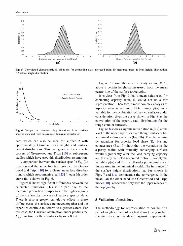
zero which can also be seen for surface 2 with
approximately Gaussian peak height and surface
height distributions. This was given in the curve fit
process of Greenwood and Tripp [10] or subsequent
studies which have used this distribution assumption.
A comparison between the surface specific F5=2 kð Þfunction and the same function provided by Green-
wood and Tripp [10] for a Gaussian surface distribu-
tion, to which Arcoumanis et al. [23] fitted a 6th order
curve fit, is shown in Fig. 6.
Figure 6 shows significant differences between the
calculated functions. This is in part due to the
increased proportion of asperities in the higher regions
of the surface for the case of surface specific data.
There is also a greater cumulative effect in these
differences as the surfaces are moved together and the
asperities continue to deform to a greater extent. For
this case, the Gaussian assumption under predicts the
F5=2 function for these surfaces by over 80 %.
Figure 7 shows the mean asperity radius, bi hð Þ,above a certain height as measured from the mean
centre-line of the surface topography.
It is clear from Fig. 7 that a mean value used for
contacting asperity radii, b, would not be a fair
representation. Therefore, a more complex analysis of
asperity radii is required. Determining b hð Þ as a
variable for the combination of the two surfaces under
consideration gives the curve shown in Fig. 8 as the
convolution of the asperity radii distributions for the
rough counter surfaces.
Figure 8 shows a significant variation in b hð Þ at thelevel of the upper asperities even though surface 2 has
a minimal radius variation (Fig. 7b). The characteris-
tic equations for asperity load share (Eq. 14) and
contact area (Eq. 15) show that the variation in the
asperity radius with mutually converging surfaces
would significantly alter the load carrying capacity
and thus any predicted generated friction. To apply the
variables b hð Þ andW hð Þ; sixth order polynomial curve
fits are used in the numerical model. The full range of
the surface height distributions has bee shown in
Figs. 7 and 8 to demonstrate the convergence to the
mean. On the other hand, the Greenwood and Tripp
model [10] is concerned only with the upper reaches of
the topography.
5 Validation of methology
The methodology for representation of contact of a
pair of rough surfaces (described above) using surface
specific data is validated against experimental
Fig. 5 Convoluted characteristic distributions for contacting pairs averaged from 10 measured areas. a Peak height distribution.
b Surface height distribution
Fig. 6 Comparison between F5=2 functions from surface
specific data and from an assumed Gaussian distribution
Meccanica
123

measurements of friction from a precision sliding
tribometer.
5.1 Sliding tribometer
A reciprocating slider tribometer is used to measure
the generated friction between the two measured
rough surfaces. A ‘strip’ (surface 2 described above)
comprising a 20 9 20 mm flat area with 45�
chamfered inlet and outlets slides on a flat sample
(surface 1 described above), the latter mounted onto a
floating flat plate, supported by frictionless bearings
and intervened from the solid base of the rig by piezo-
resistive load cells (Fig. 9). The floating plate is
dragged by the sliding contact conjunction, lubricated
by 1 ml of base oil applied to the plate surface,
furnishing a very thin lubricant film and significant
asperity interactions. The drag force (generated
Fig. 7 Asperity radius
distributions for the counter
surfaces 1 and 2, averaged
from 10 measured areas.
a Surface 1. b Surface 2
Fig. 8 Convoluted asperity
radius and curvature
distributions averaged from
10 measured areas
Meccanica
123
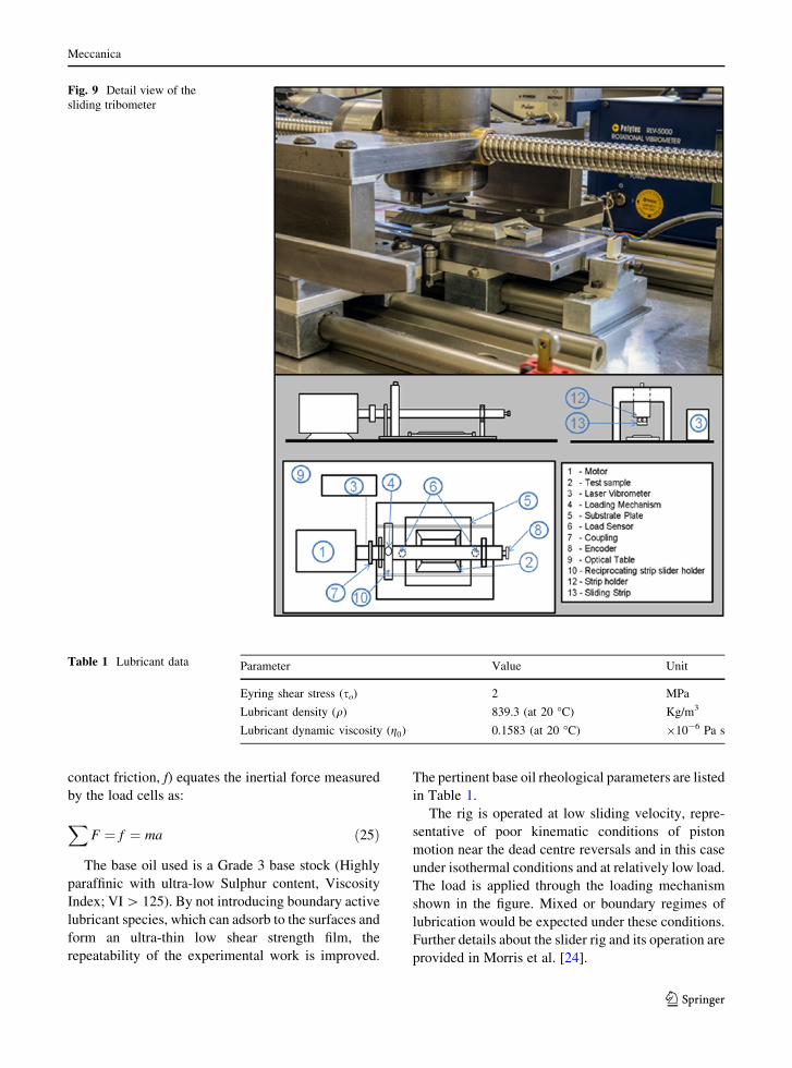
contact friction, f) equates the inertial force measured
by the load cells as:
XF ¼ f ¼ ma ð25Þ
The base oil used is a Grade 3 base stock (Highly
paraffinic with ultra-low Sulphur content, Viscosity
Index; VI[ 125). By not introducing boundary active
lubricant species, which can adsorb to the surfaces and
form an ultra-thin low shear strength film, the
repeatability of the experimental work is improved.
The pertinent base oil rheological parameters are listed
in Table 1.
The rig is operated at low sliding velocity, repre-
sentative of poor kinematic conditions of piston
motion near the dead centre reversals and in this case
under isothermal conditions and at relatively low load.
The load is applied through the loading mechanism
shown in the figure. Mixed or boundary regimes of
lubrication would be expected under these conditions.
Further details about the slider rig and its operation are
provided in Morris et al. [24].
Fig. 9 Detail view of the
sliding tribometer
Table 1 Lubricant data Parameter Value Unit
Eyring shear stress (so) 2 MPa
Lubricant density (q) 839.3 (at 20 �C) Kg/m3
Lubricant dynamic viscosity (g0) 0.1583 (at 20 �C) 910-6 Pa s
Meccanica
123

Relatively low load and large apparent contact area,
A (contacting face of the strip) yields insufficient
lubricant pressures to cause any elasto-hydrodynamic
deformation of the surfaces. Furthermore, any lubri-
cant film thickness, h, above the mean surface height
of topography, d, is expected to be quite thin, yielding
a mixed regime of lubrication.
5.2 The numerical model
The generated friction under the anticipated mixed-
hydrodynamic regime of lubrication is obtained as:
f ¼ fv þ fb ð26Þ
where, the total friction, f is as the result of contri-
butions due to the viscous shear of a thin lubricant film
and boundary friction due to the interaction of
asperities on the counterfaces of the contacting
surfaces.
The viscous friction force is obtained as follow:
fv ¼Z L
0
Z b=2
�b=2
� h
2r*
p� Ugh
��������dxdy ð27Þ
Boundary friction is due to the interaction of
counterface asperities, as well as any pockets of
lubricant entrapped between them, which are assumed
to be subject to the limiting Eyring [25] shear stress as
[9]:
fb ¼ s0 ~Aþ 1~P ð28Þ
where, ~A is given by Eq. (15). This value is clearly
different for the measured surface specific topography
and that based on the assumption of Gaussian distri-
bution of Greenwood and Tripp [10] model. There-
fore, the resultant friction predicted for an assumed
Gaussian peak height distribution, using Greenwood
and Tripp [10] model and that for peak height
distribution determined using the measured surface
data are compared with the directly measured friction
using the experimental rig.
The first term on the right-hand side of Eq. (28)
represents the non-Newtonian shear of thin pockets
of lubricant. The second term corresponds to the
direct interaction of asperities. 1 is the coefficient ofshear strength of asperities, measured using an atomic
force microscope in the lateral force mode [8]. The
Eyring shear stress is given in Table 1, and 1 ¼ 0:17
[26].
It is clear that the lubricant film thickness, h is
required in order to predict the viscous friction
contribution in Eq. (27). Therefore, a quasi-static load
balance must be sought between the contact load
carrying capacity, comprising asperity load share and
any hydrodynamic lubricant reaction against the
applied load, thus:
W ¼ Why þ ~P dð Þ ð29Þ
The hydrodynamic lubricant film reaction is
obtained as:
Why ¼ZZ
pdxdy ð30Þ
The hydrodynamic generated pressure distribution
is obtained through solution of Reynolds equation:
o
ox
qh3
6gop
ox
� �þ o
oy
qh3
6gop
oy
� �¼ U
o qhð Þox
þ 2o qhð Þot
ð31Þ
where, U is the sliding velocity of the strip in the x-
direction. The strip is of finite length, thus the
Poiseuille side-leakage flow due to pressure gradient
in the lateral y-direction is also taken into account. The
final term on the right-hand side of the equation takes
the squeeze film effect into account due to the transient
nature of the problem.
The lubricant film shape is given as:
h x; yð Þ ¼ h0 þx2
2Rþ d x; yð Þ ð32Þ
where, h0 is the initial gap. As already noted there is no
localised elastohydrodynamic deformation of the
contacting surfaces for the relatively low generated
pressures, thus: d x; yð Þ ffi 0.
The boundary conditions used for the solution of
Reynolds equation are:
p x¼�b=2ð Þ ¼ Patm; p x¼cð Þ ¼ Pcav andop
ox
����x¼cð Þ
¼ 0
ð33Þ
These correspond to atmospheric pressure at the
inlet (x ¼ �b=2), where b is the effective face-width of
the sliding strip and Swift–Stieber boundary condi-
tions at the film rupture point at the contact exit
constriction (x ¼ c), where the cavitation pressure is
that of the lubricant at the environmental temperature
Meccanica
123
of 20 �C. In this study the cavitation pressure is
assumed to be equal to the atmospheric pressure.
In the lateral direction (side-leakage direction):
p y¼0ð Þ ¼ p y¼lð Þ ¼ Patm ð34Þ
The rheological properties of the lubricant vary
with pressure in the current isothermal analysis. The
relationships given by Dowson and Higginson [27]
and Houpert [28] are utilised to take into account the
variations of lubricant density and dynamic viscosity
with pressure and temperature as:
q ¼ q0 1þ 6� 10�10 p� patmð Þ1þ 1:7� 10�9 p� patmð Þ
� ð35Þ
and:
g ¼ g0exp
�ln g0 þ 9:67
�
1þ 5:1� 10�9 p� patmð Þ �Z�1
� ��ð36Þ
where:
Z ¼ a5:1� 10�9 ln g0 þ 9:67ð Þ ð37Þ
A second order finite difference method is used to
solve Reynolds equation by utilising Point-Successive
Over-Relaxation scheme. During the iterations the
lubricant properties are also updated. The procedure
used, including for convergence criteria, are described
in Rahmani et al. [29].
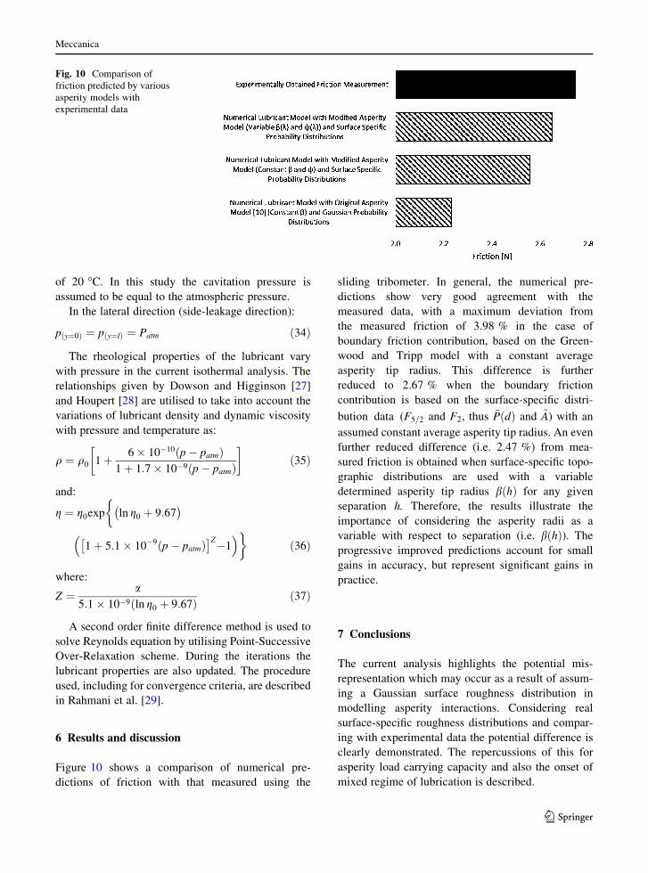
6 Results and discussion
Figure 10 shows a comparison of numerical pre-
dictions of friction with that measured using the
sliding tribometer. In general, the numerical pre-
dictions show very good agreement with the
measured data, with a maximum deviation from
the measured friction of 3.98 % in the case of
boundary friction contribution, based on the Green-
wood and Tripp model with a constant average
asperity tip radius. This difference is further
reduced to 2.67 % when the boundary friction
contribution is based on the surface-specific distri-
bution data (F5=2 and F2, thus ~P dð Þ and ~A) with an
assumed constant average asperity tip radius. An even
further reduced difference (i.e. 2.47 %) from mea-
sured friction is obtained when surface-specific topo-
graphic distributions are used with a variable
determined asperity tip radius b hð Þ for any given
separation h. Therefore, the results illustrate the
importance of considering the asperity radii as a
variable with respect to separation (i.e. b hð Þ). Theprogressive improved predictions account for small
gains in accuracy, but represent significant gains in
practice.
7 Conclusions
The current analysis highlights the potential mis-
representation which may occur as a result of assum-
ing a Gaussian surface roughness distribution in
modelling asperity interactions. Considering real
surface-specific roughness distributions and compar-
ing with experimental data the potential difference is
clearly demonstrated. The repercussions of this for
asperity load carrying capacity and also the onset of
mixed regime of lubrication is described.
Fig. 10 Comparison of
friction predicted by various
asperity models with
experimental data
Meccanica
123

It is also clear that the method of considering
variation in asperity radii at different separations,
developed here, offers additional improvements for
surface analysis and modelling. The use of measured
surface-specific distribution and separation-dependent
variable asperity radii are the main contributions made
to knowledge in this paper. The developed methodol-
ogy also shows very good agreement with experimen-
tal measurements of friction.
Acknowledgments The authors would like to thank the UK
Engineering and Physical Sciences Research Council (EPSRC)
for the sponsorship of this research under the Encyclopaedic
Program Grant (www.encyclopaedic.org).
Open Access This article is distributed under the terms of the
Creative Commons Attribution 4.0 International License (http://
creativecommons.org/licenses/by/4.0/), which permits unre-
stricted use, distribution, and reproduction in any medium,
provided you give appropriate credit to the original
author(s) and the source, provide a link to the Creative Com-
mons license, and indicate if changes were made.
References
1. Dowson D (ed) (1982) Tribology of reciprocating engines.
In: Proceedings of 9th Leeds–Lyon symposium on tribol-
ogy, 1982
2. Balakrishnan S, Rahnejat H (2005) Isothermal transient
analysis of piston skirt-to-cylinder wall contacts under
combined axial, lateral and tilting motion. J Phys D Appl
Phys 38(5):787
3. Tipei N (1968) Boundary conditions of a viscous flow
between surfaces with rolling and sliding motion. Trans
ASME J Tribol 90(1):254–261
4. Shahmohamadi H, Mohammadpour M, Rahmani R, Rah-
nejat H, Garner CP, Howell-Smith S (2015) On the
boundary conditions in multi-phase flow through the piston
ring-cylinder liner conjunction. Tribol Int 90:164–174
5. Furuhama S, Sasaki S (1983) New device for the mea-
surement of piston frictional forces in small engines. SAE
technical paper, no. 831284, 1983
6. Bolander NW, Steenwyk BD, Sadeghi F, Gerber GR (2005)
Lubrication regime transitions at the piston ring-cylinder
liner interface. Proc IMechE Part J J Eng Tribol 219(1):
19–31
7. Gore M, Theaker M, Howell-Smith S, Rahnejat H, King PD
(2014) Direct measurement of piston friction of internal-
combustion engines using the floating-liner principle. Proc
IMechE Part D J Automob Eng 228(3):344–354
8. Styles G, Rahmani R, Rahnejat H, Fitzsimons B (2014) In-
cycle and life-time friction transience in piston ring–liner
conjunction under mixed regime of lubrication. Int J Engine
Res 15(7):862–876
9. Teodorescu M, Kushwaha M, Rahnejat H, Rothberg SJ
(2007) Multi-physics analysis of valve train systems: from
system level to microscale interactions. Proc IMechE Part
K J Multi Body Dyn 221(3):349–361
10. Greenwood J, Tripp J (1970) Contact of two nominally flat
rough surfaces. Proc IMechE J Mech Eng Sci 185:625–633
11. Greenwood J, Williamson JBP (1966) Contact of nominally
flat surfaces. Proc R Soc 295:300–319
12. Hisakado T (1974) Effect of surface roughness on contact
between solid surfaces. Wear 28(2):217–234
13. Bush AW, Gibson RD, Keogh GP (1976) Strongly aniso-
tropic rough surfaces. Trans ASME J Tribol 101(Part
1):15–20
14. McCool JI (1986) Comparison of models for the contact of
rough surfaces. Wear 107(1):37–60
15. Pullen J, Williamson JBP (1972) On the plastic contact of
rough surfaces. Proc R Soc 327(1569):159–173
16. Cheng HSA (1970) Numerical solution of the elastohydro-
dynamic film thickness in an elliptical contact. Trans ASME
J Tribol 92(Part 1):155–161
17. ChongWWF, Teodorescu M, Rahnejat H (2013) Nanoscale
elastoplastic adhesion of wet asperities. Proc IMechE Part
J J Eng Tribol 227(9):996–1010
18. Ma Z, Henin A, Bryzik W (1997) A model for wear and
friction in cylinder liners and piston rings. Tribol Trans
49(3):315–327
19. Mishra PC, Rahnejat H, King PD (2009) Tribology of the
ring—bore conjunction subject to a mixed regime of
lubrication. Proc IMechE Part C J Mech Eng Sci
223(4):987–998
20. Liu G,Wang Q, Lin C (2006) A survey of current models for
simulating the contact between rough surfaces. Tribol Trans
42(3):581–591
21. Teodorescu M, Kushwaha M, Rahnejat H, Taraza D (2005)
Elastodynamic transient analysis of a four-cylinder valve-
train systemwith camshaft flexibility. Proc IMechE Part K J
Multi Body Dyn 219:13–25
22. Peklenik J (1967) Paper 24: new developments in surface
characterization and measurements by means of random
process analysis. Proc IMechE Conf 182(11)
23. Arcoumanis C, Ostovar P, Mortier R (1997) Mixed lubri-
cation modelling of Newtonian and shear thinning liquids in
a piston-ring configuration. In: SAE technical paper, 1997,
pap no. 972924:35
24. Morris N, Leighton M, De la Cruz M, Rahmani R, Rahnejat
H, Howell-Smith S (2015) Combined numerical and
experimental investigation of the micro-hydrodynamics of
chevron-based textured patterns influencing conjunctional
friction of sliding contacts. Proc IMechE Part J J Eng Tribol
229(4):316–335
25. Eyring H (1936) Viscosity, plasticity, and diffusion as
examples of absolute reaction rates. J Chem Phys 4(4):
283–291
26. De la Cruz M, Chong WWF, Teodorescu M, Theodossiades
S, Rahnejat H (2012) Transient mixed thermo-elastohy-
drodynamic lubrication in multi-speed transmissions. Tribol
Int 49:17–29
27. Dowson D, Higginson GR (1959) A numerical solution to
the elasto-hydrodynamic problem. J Mech Eng Sci 1(1):
6–15
Meccanica
123

28. Houpert L (1985) New results of traction force calculations
in elastohydrodynamic contacts. Trans ASME J Tribol
107(2):241–245
29. Rahmani R, Theodossiades S, Rahnejat H, Fitzsimons B
(2012) ‘‘Transient elastohydrodynamic lubrication of rough
new or worn piston compression ring conjunction with an
out-of-round cylinder bore. Proc IMechE Part J J Eng Tribol
226(4):284–305
Meccanica
123