Surface hydrology in global river basins in the Off-line

Land-surface GEOS Assimilation (OLGA) system

Michael G. Bosilovich

Universities Space Research Association, Seabrook, Maryland

Runhua Yang

General Sciences Corporation, Seabrook, Maryland

Paul R. Houser

Hydrologic Sciences Branch / Data Assimilation Office, NASA/GSFC Code 974,

Greenbelt, Maryland

jj's_ ........ :::

Short title: SURFACE HYDROLOGY IN GLOBAL RIVER BASINS

2

Abstract.

Land surfacehydrology for the Off-line Land-surfaceGEOS Analysis (OLGA)

system and Goddard Earth ObservingSystem (GEOS-1) Data Assimilation System

(DAS) hasbeenexamined using a river routing model. The GEOS-1 DAS land-surface

parameterization is very simple, using an energy balance prediction of surface

temperature and prescribed soil water. OLGA uses near-surface atmospheric data from

the GEOS-1 DAS to drive a more comprehensive parameterization of the land-surface

physics. The two global systems are evaluated using a global river routing model. The

river routing model uses climatologic surface runoff from each system to simulate the

river discharge from global river basins, which can be compared to climatologic river

discharge. Due to the soil hydrology, the OLGA system shows a general improvement

in the simulation of river discharge compared to the GEOS-1 DAS. Snowmelt processes

included in OLGA also have a positive effect on the annual cycle of river discharge

•and source runoff. Preliminary tests of a coupled land-atmosphere model indicate

improvements to the hydrologic cycle compared to the uncoupled system. The river

routing model has provided a useful tool in the evaluation of the GCM hydrologic cycle,

and has helped quantify the influence of the more advanced land surface model.

i. Introduction

Data assimilation systems have provided the climate and meteorology community

with long-term atmospheric data sets that cover the globe and maintain consistency

in time [Bengsston and Shukla, 1989; Daley, 1991]. The Goddard Earth Observing

System (GEOS-1) Data Assimilation System (DAS) produced one of the first long-term

reanalyses to use a consistent modeling and assimilation system [Schubert et al., 1993].

In this system, the prescribed land-surface wetness was computed from a bucket model

forced with observations of monthly mean precipitation and near-surface atmospheric

temperature [see, Mintz and Serafini, 1992; Schemm et al., 1992; Mintz and Walker,

1993]. While the prescribed soil wetness has some advantages, the resulting GEOS-1

DAS land-surface hydrologic budget was not balanced during the model integration.

Recently, the Off-line Land-surface GEOS Assimilation (OLGA) system has been

developed to provide more detailed surface data over the globe. OLGA is a global land

surface model driven by near-surface atmospheric data from the GEOS DAS reanalysis.

The Koster and Suarez [1992, 1996] Mosaic land-surface model provides the core of the

surface physical parameterizations including surface heat and water budgets.

The present study evaluates the influence of OLGA's active land surface calculations

compared to the GEOS-1 prescribed soil wetness on the modeling of global climate

land-surface hydrology. An important and sensitive component of surface hydrology is

the runoff water. Here, we define the source runoff water as the runoff water that is

produced from the model hydrology at the GCM grid. While runoff water observations

are generally not available, the discharge of water at river mouths is routinely observed.

Note the distinction between source runoff water and river discharge.

In order to close the general circulation model (GCM) hydrology, the river routing

model developed by Miller et al. [1994] routes GCM source runoff water through a

river system to simulate the river discharge of numerous basins around the Earth. The

comparison of model and observed river discharge is a rigorous validation of the surface

4

model's ability to simulate important physical processessuchas snowmelt.

In the OLGA and GEOS-1simulations, interaction betweenthe surfacesoil water

and precipitation does not occur. While OLGA soil water is predicted basedon

precipitation, it doesnot changethe precipitation. Soil water can influenceprecipitation

processesin a variety of ways [Mintz, 1984;Beljaars et al., 1996; Bosilovich and Sun,

1998], and ultimately, the interactions must be included in numerical simulations. The

next generation of the GEOS-DAS will incorporate the Mosaic LSM as its surface

boundary. The interactive surface model has already been successfully implemented into

the GEOS-GCM. We will also present hydrology results from the coupled GEOS-GCM

and LSM.

2. Methodology

In this section, we summarize OLGA and GEOS-1 DAS specifically focusing on the

surface hydrology modeling strategies. The river routing model and the observations of

precipitation and river discharge are also described.

2.1. Off-line Land-surface GEOS Assimilation (OLGA) System

The Off-line Land surface GEOS Assimilation (OLGA)system [Houser et al., 1998]

is being developed as a testbed for developing land data assimilation strategies for

the fully coupled GEOS-DAS. Therefore, to the greatest extent that is reasonable, the

OLGA system has been designed to mimic the fully-coupled system, with the vision

of eventually implementing techniques developed off-line into the full GEOS-DAS.

The OLGA system is proving to be an excellent resource for efficiently testing new

land surface data assimilation strategies, and allows for the off-line replacement of

often biased GCM land surface forcing fields (such as precipitation and radiation) with

observed quantities.

The OLGA system was implemented globally over land at a 2° x 2.5 ° resolution for

the 14yearsof available GEOS-1DAS reanalysisforcing (1981 through 1995). The 3

hour GEOS-1DAS forcing data waslinearly interpolated in time to the 5 minute OLGA

time step. The International Satellite Land-SurfaceClimatology Project (ISLSCP)

initiative 1 land cover definitions specify vegetation in OLGA [Meeson et al., 1995;

Sellers et al., 1995]. A five year OLGA simulation was used to spin-up the inital state

for the present simulation. The OLGA surface data sets are currently being offered as a

supplement to the inactive land surface present in the GEOS-1 DAS.

Mosaic [Koster and Suarez, 1992, 1996] is the current Land Surface Model (LSM)

implemented in OLGA. The Mosaic model is based on sound, well- accepted theory

that has been proven by: (1) its superior performance in several model intercomparison

studies including the Project for the Intercomparison of Land Surface Schemes (PILPS)

[Henderson-Sellers et al., 1993]; (2) its ability to produce stable land surface conditions

and realistic climate simulations in the NASA/GSFC Aries GCM [Suarez et al, 1996;

and (3) the high correlation between Mosaic predictions and in-situ observations of

surface fluxes and states made during several intensive field campaigns.

The Mosaic LSM was originally derived from the Simple Biosphere (SiB) model

developed by Sellers et al. [1986]. Mosaic, however, accounts for sub-grid scale

heterogeneity by dividing each GCM grid into homogeneous sub-regions. Furthermore,

each sub-region is associated with a shallow profile of model atmospheric grid points.

This permits partial surface atmosphere interactions, but only near the surface, not

with the large-scale environment.

The data that drive OLGA are the atmospheric state (temperature, moisture

and wind), the downwelling shortwave and longwave radiation, surface pressure and

precipitation. Mosaic maintains eight prognostic variables, which include the surface

skin and deep soil temperatures, the canopy vapor pressure, and the moisture content

of the snowpack, interception reservoir and soil layers. A percentage of the incoming

radiative energy to the land surface is reflected, and the remainder that is absorbed

6

is partitioned into upwelling longwaveradiation, snowmelt, and sensible,latent, and

ground heat fluxes. The partitioning of energy fluxes is controlled by a seriesof

resistancesthat vary with environmental stress,and heat flow into the soil is performed

using a force-restoremethod. Precipitation falling on the land surfaceis partitioned

into canopyinterception, surfacerunoff, or infiltration into the first of three soil layers.

Water diffusesbetween these three layers,and can percolateout of the third layer.

Water can be evaporatedfrom the interception reservoirand the snowpack,and can be

extracted by plants from the top two soil layers for transpiration. Koster and Suarez

[1996] discuss the water and energy conservation calculations in greater detail. For the

present work, the calculation of runoff water is described below.

The rate of total source runoff, R, is generated in Mosaic as the sum of the surface

runoff rate, Rs, and the baseflow or moisture diffusion flux out of the bottom of the

lowest soil layer, Qa_:

n=ns+Q3 (1)

The surface runoff rate, R_, is equal to the rate of rain throughfall, PT, less

infiltration:

= Pr- w,At (2)

where WI is the moisture in the top layer, At is the time step length, and the subscript

old denotes quantities calculated at the previous time step. The moisture in the top

layer is updated by adding the smaller of either the throughfall onto dry soil, PT-eru, or

the unused top layer moisture capacity, Wl-_de:

W1 = [W1]old + min(PT-drv, WI-_aa) (3)

Mosaic soil hydrology calculations are divided into two sub-areas, one that is fully

saturated and the other whose degree of saturation is Wl-eq/Wl-s_t. Wl-eq is the

water content in the top soil layer that would be in equilibrium (according to Richards

equation) with the water content in the middle soil layer, and Wl-s_t is the moisture

............................................................................:: _::::_:-_:::::::_:::_:___........_:: _:: :_:_::__::_:_:_:_:__:_ _::i:ii_!_<ii!_i_!_i:_:i_<_::_::_i_i_i_i_i_iT!i_i_i_iii_i_!_i_i_i_i_i_!_ii!_i_iiiii!ii_i_i_i_!!i!i_iii_i_i!ii_i_!ii_i!i_iii!!_ii_iiiiiiiiiiiiii_iiii_iii_i_i!iii_iii_i_iii_iiiii_ii_i_ii_iii_iiiiiii_i;iiiii_i_ii_iiiiiiiiiiii_iiiiiiiiiiiiiiiii_iiiiiii_

holding capacity of the top soil layer. Given that W1 is the total amount of water in the

top soil layer, the saturated fraction, fs_t, can be computed as:

W1 -Wl__q

= >

0 W 1 <Wl_eq

Then, the throughfall mass falling on the dry fraction is:

PT-dry = PT(1 -- f_at)At

and the unused moisture capacity of the top layer is:

(4)

(5)

Wl-_dd = f(l/Vl-_t- Wl__q)(1 - f_at) (6)

where f is the fractional coverage of precipitation.

Percolation out of the bottom of the lowest soil layer, Q3_o, is computed with a

bulk form of Richards equation in which only gravitational drainage operates, and the

presence of bedrock is allowed to reduce the flow:

q3_ = p_K3 sin(O) (7)

where 0 is the bedrock angle, /(3 is the hydraulic conductivity of the lowest soil layer,

and p_ is the density of liquid water.

2.2. Goddard Earth Observing System (GEOS)

The GEOS-1 DAS has produced a multi-year global atmospheric data set for use

in climate and weather studies [Schubert et al., 1993]. The GEOS-1 GCM is described

by Takacs et al. [1994] and Molod et al. [1996]. Pfaendtner et al. [1995] document the

DAS. Bosilovich and Schubert [1998] discuss the GEOS-1 DAS surface parameterization

in detail.

A simple bucket model specifies the GEOS-1 DAS monthly mean soil wetness

off-line. The bucket model uses observed monthly mean precipitation and temperature

.........................................._:_ ...............<, _.........__> _,_:,_: _<__:________:_:__,:::::_i__<_<_i:i_i_<_:<<__!_i__<ii!_!!i_:!_i_i_iii̧!!i!_i_!_!!_ii!_iiiiiii_!_:iiiiiiii!ii:_i_iiii!!_ii_i_;!i!ii_!;iiliiiii_iiii_iiiiiii<:iiiiiiiii!i_i_iiiiiiiiiiiii!i_i_ii<ii!i_iii_iiiiiiiiiiiii_i_iiiiiiiiii;ii_i_iiiiiiiiii;iiiiiiiiiiiii¸

as input [Schemm et al., 1992], similar to the procedure of Mintz and Serafini [1992],

The prescribed soil wetness should provide lower boundary forcing that resembles

observations and cannot drift toward unrealistic values. While modeled precipitation

may be biased, the bias will not feed back into the atmospheric system through the soil

wetness. However, without an interactive hydrologic balance at the surface, the long!

term integration of evaporation no longer depends on the modeled precipitation. Runoff

water is diagnosed from monthly mean soil water, precipitation and evaporation after

the completion of the model integration.

For each month during the period from January 1985 through December 1993,

monthly mean runoff is computed by,

OWRo= P-E- --

Ot " (8)

Here, P and E are the monthly mean precipitation and evaporation, respectively. Ro is

the source runoff. While the monthly mean storage of water (OW/Ot) is generally small,

it cannot be neglected in the annual cycle. Because the storage of water is prescribed

prior to the integration of the GEOS-1 reanalysis, this diagnostic computation can yield

Ro < 0. Uncertainty of the evaporation based on the prescribed soil wetness and the

inability of the storage of w.ater to react to P - E lead to negative values of runoff, which

is unrealistic in the climate system [See also, Arpe, 1998]. If at a grid point Ro < O,

then that month's value of runoff is set to zero, and the negative value is integrated into

a residual variable. The residual variable is saved to indicate the amount of imbalance

in the GEOS surface hydrology. Hence, only positive values of runoff from Eq. 8 are

included in the computation of GEOS-1 climate annual cycle of runoff.

Presently, the Mosaic land surface model (LSM) [Koster and Suarez, 1992, 1996] is

being incorporated into the GEOS DAS. The LSM is identical to that applied in OLGA.

Hence, future versions of the GEOS system will not be limited by the same deficiencies

noted in this section. Some preliminary results of the GEOS GCM coupled with Mosaic

9

LSM will alsobe presented.

2.3. River Routing Model

The river routing model was developedto provide closureto GCM hydrology

budgets and to allow validation of GCM sourcerunoff [Miller et al., 1994]. Climate

mean source runoff of GCMs (Ro) provides the forcing for the river routing (again,

noting the difference between source runoff and river discharge defined earlier). In order

to move the water from grid spaces to the river mouth, the routing model requires an

algorithm for the river mass flow and a river direction file based on the topographic

gradient. Miller et al. [1994] provide a complete list and map of all the river basins.

Forty-seven river basins are defined in the river routing model with 2 ° x 2.5 ° resolution.

The flux of water from a grid box (F in kg s -I) is given by,

U

F = M x _. (9)

Where, M is the river mass above the sill depth, dis the mean distance between the grid

box and its downstream neighbor, and u is an effective flow rate of water from a grid

box to its downstream neighbor, depending on the downstream topography gradient.

During a time step, the change in river mass in a grid box is given by,

M(t + At) - M(t) = Ro + AtEFzN - AtFouT° (10)

Where, FouT is the flux of water that leaves a grid box, and EFzN is the flux of water

entering a grid box. Eventually, the water is moved to the river mouth, where it is

defined as the river discharge.

The resulting river discharge comparison with observations identifies strengths and

weaknesses in the GCM hydrology, but it must be carefully examined. The river routing

model cannot ameliorate the effect of errors in GCM evaporation and precipitation on

the river discharge. In addition, several river flow parameters are specified globally, for

10

lack of detailed observations. Someprocessesarenot explicitly included in the river

routing model, suchas freezingrivers (though the MosaicLSM doesfreezesoil water)

and ice flow.

2.4. Observations

We use two types of observeddata for verification: river dischargefrom over

thirty-seven river basinsand gridded precipitation. The monthly mean river discharge

data wereprovided by Global Runoff Data Center,Federal Institute of Hydrology,

Germany. The climatological monthly mean river dischargewere computedfor the

period of January 1979to December1988. The observedmonthly meanprecipitation

were mergedMicrowaveSoundingUnit version-1overoceansblendedwith rain gauge

data over land at 4° x 5° resolution. The climatological monthly mean valueswere

computed for the same10years asthe river dischargedata [Lau et al., 1996]. These

precipitation data over land were also used to compute the GEOS-1 soil wetness

boundary condition [Schemm etal., 1992].

For comparison purposes, we approximate the basinwide observed evaporation using

the climate mean river discharge and basin averaged precipitation observations. It is

assumed that in a climate mean average the river discharge approximates area averaged

grid space runoff, and that the climate change of soil water is negligible. Therefore, by

averaging equation 8 for the annual cycle, the climate mean basinwide evaporation can

be computed by

E = P- Re. (11)

All the uncertainty in both precipitation and river discharge (Rd) will then be reflected

in E.

3. Results

11

3.1. Basinwide Climate Hydrology

We approximate the annual mean basinwide observed evaporation assuming that

it is equal to the difference of annual mean precipitation and river discharge. Figure

1 shows the climate mean evaporation and evaporative fraction (E/P) for 25 of the

modeled river basins (sorted by decreasing observed river discharge). In most of the

basins, and especially the largest, GEOS-1 tends to over estimate the evaporation.

While OLGA's evaporation tends to be less than (or equal to) that of GEOS-1, it is still

larger than the observed residual evaporation in many basins. This may be related to

GEOS-1 small overestimate of precipitation in many of the river basins.

The lack of surface hydrology balance in GEOS-1 is apparent in the basinwide

climate mean evaporative fraction (Figure lb). In many basins, GEOS-1 evaporative

fraction is unrealistic for a climate mean (E/P > 1). OLGA's evaporative fraction

tends to be closer to observations and it is always less than one for a basinwide climate

average. The reason for this drop in evaporation is because OLGA conserves water in

the soil, and in GEOS-1, the soil water does not interact with the evaporation.

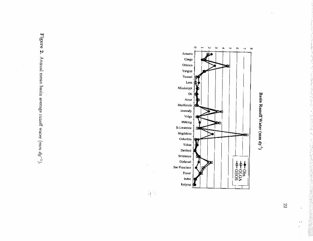
Figure 2 shows the observed annual mean river discharge observations (area

averaged) and model basinwide average grid point runoff. There are a few river basins

where OLGA and GEOS clearly have difficulty to simulate the hydrology. However,

there are more basins where the differences from observations are not very large. Because

the GEOS-1 DAS runoff was diagnosed by using a hydrologic balance (neglecting the

negative values of runoff), the annual mean of the GEOS-1 runoff is similar to that of

OLGA. As we will show in the next section, the major differences between the two cases

are in the representation of the annual cycle.

IFigure 11

IF_gure 2]

.............................. :'_ ::_:: : :<:_:<: <:_:_:_::<..... _ __: ::__::_:,__:̧k_:¸¸<: _:: ::_ _:_: _ :_:! :_:< i_: k i_<:_!!i_!_<_C_i_i_!_!_!_iii_?_<i_!!C!_i_iii!_iii_!i!_!_i_ii_ii_ii_!i_i_i_i_i!iiiii_ii_ii_i!iiiii_i_i_!_i_i!ii_i_i_i_iiiiiii_iiiiiiiii!_

12

3.2. OLGA and GEOS-1 DAS Annual Cycles

While there may be many sources of uncertainty in the simulated river discharge

(as discussed previously), much may still be learned about the model's hydrology. For

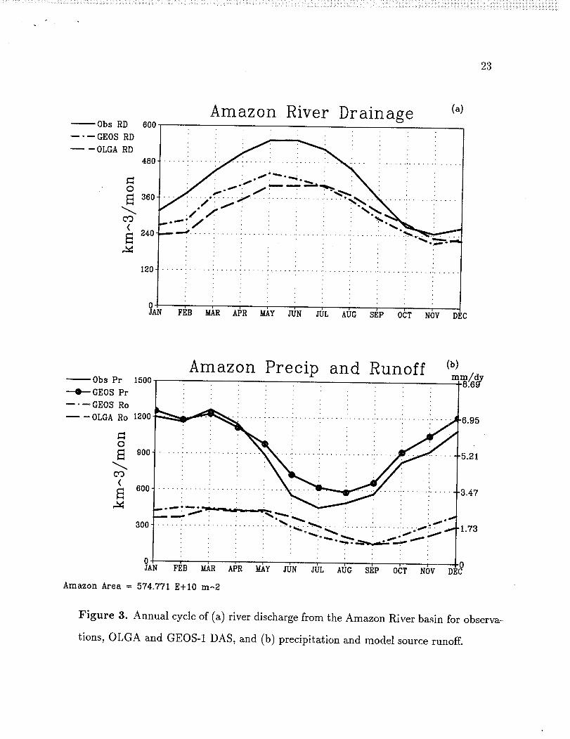
example, Amazon river discharge is particularly difficult to simulate. Lau et al. [1996]

find that many GCM's cannot generate as much river discharge as observed. Also, using

the river routing model, coupled with the Goddard Institute for Space Studies GCM,

Miller et al. [1994] strongly underestimate the Amazon's river discharge. In the present

study, the Amazon precipitation is very large but comparable to observation (Figure 3).

The source runoff for both OLGA and GEOS-1 are very similar, with OLGA slightly

lagging behind GEOS-1. Overall, there are only small differences between the two

models' river discharge.

In the Congo river basin, GEOS-1 tends to overestimate precipitation, leading to

the overestimate of river discharge in both OLGA and GEOS-1 (Figure 4). However,

the phase of OLGA river discharge has improved compared to GEOS-1. While the more

detailed land-surface processes in OLGA help improve the river discharge in the Congo,

this is not always the case (as in the Amazon).

As discussed by Boyle [1998], GCMs tend to over estimate spring and summer

rainfall amounts in the United States. This has been known for some time in the

GEOS-1 DAS [Schubert et al., 1995], and it is quite apparent in these results (Figure 5).

In the Mississippi river basin, the high summer precipitation dominates the simulate

river discharge. Beljaars et al. [1996] results suggest that better representation of the

surface water content can improve the simulation of precipitation. The poor summer

precipitation in GEOS-1 could be related to the simplistic surface representation.

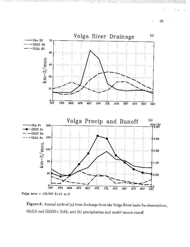
The northern river basins in OLGA exhibit substantial improvement of both source

runoff and river discharge. The Volga river basin is a good example (Figure 6), but

this result is also true for other basins (Amur, Ob and somewhat noticeable in the

Mississippi). The snowmelt clearly affects the river discharge simulation, but there are

[Figure 31

IFigure 41

IFigure 51

l Figure 61

............................. .......................................:::::_:::::_::_:_:::_:_:::_:_:_:__:_: :_:::_:::_:::_ ::_::_:_::,_:_:__:__: :::::__::___:_:_:_:_i_:_::_:_::_:i_:_i__:ii!i_i:i_i_iii_!_il!_i_ii:ii_!ii_!!ii:__!:iili!iii_iiliii:_ii!iiiii!__:______::ii!iiiiiiiii_iiiiiliiiiiiiiiii!iiiiiiiiiiiiiiiiiiii_i_i!i_i!i_i!iii_iiiii!iii_i!i_i___i_i_i_iii_i_iii_i!iiiiiiiiiiiiiiiii_iiiiii_iiiiiiiiiiiii_iiiiiiiiiiiiiiji

13

still differences between OLGA and observations. This could be the result of either

less winter precipitation (snow) or an underestimate of the river flow rates in the river

routing model. The GEOS-1 system, however, does not include snowmelt processes.

The influence of the Mosaic LSM snowmelt in OLGA is quite apparent in the source

runoff, especially compared to GEOS-1 (March and April source runoff in Figure 6b).

3.3. GEOS GCM with Interactive Land Surface Processes

In the previous discussion, the coupled land-surface interactions are not included in

either the OLGA or GEOS-1 systems. The interaction between surface and atmosphere

will influence the precipitation, evaporation and the river discharge (among other

processes). An ongoing effort to incorporate the Mosaic LSM into the GEOS GCM has

produced some preliminary results. Here, we present results from the GCM coupled

with the Mosaic LSM (GCM-LSM) and GCM with the same surface parameterization

as in GEOS-1 (Control). The GCM resolution is 4 ° x 5 °, and both GCM cases were

integrated for 5 years. Note that the GEOS-1 DAS reanalyses includes observational

data assimilated into the GCM global system. In this experiment, the GCM simulations

do not include the assimilated observations.

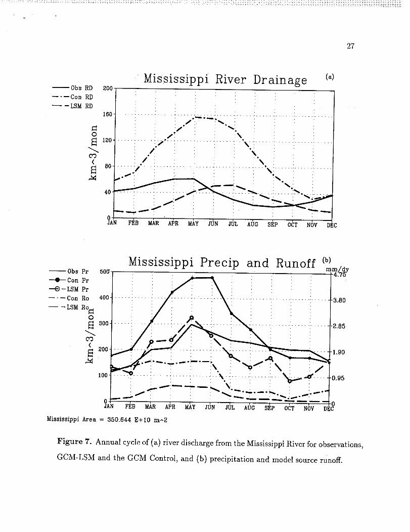
The influence of the coupled system on the Mississippi river basin precipitation is

quite clear (Figure 7). In the Control simulation, the precipitation is very large in spring

and summer, much like that of GEOS-1, leading to a substantial overestimate of the

river discharge. With the coupled LSM, the spring and summer precipitation is much

less than control and closer to observations. However, autumn precipitation, which is a

valuable recharge source in the annual hydrologic cycle, is underestimated. This leads

to low springtime river discharge. For the climate mean over the entire annual period,

the both precipitation and river discharge are much closer to observed than the Control.

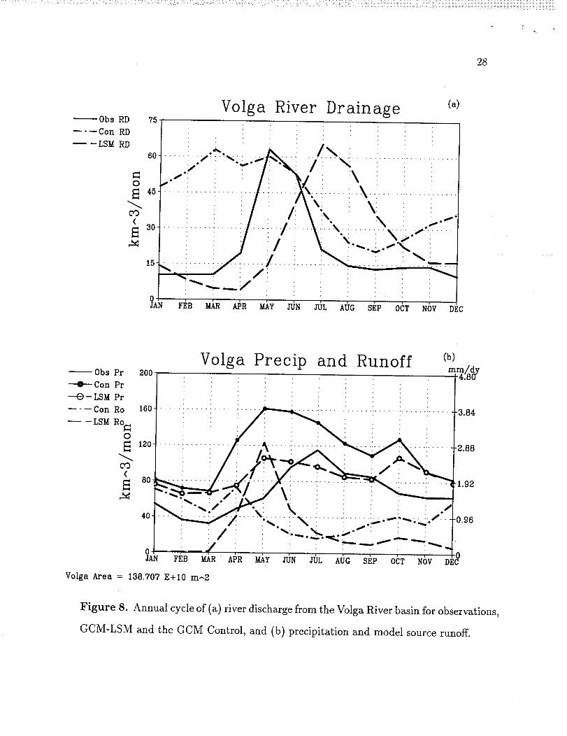
The GCM-LSM simulation of snowmelt processes is much better than the Control

simulation. The Control Volga river basin exhibits large river discharge in the winter

1Figure 71

14

due to the lack of simulated snow processes. The GCM-LSM, however, includes snow

processes, and produces a strong snowmelt signature in the model source runoff during

late spring (Figure 8). The resulting simulated river discharge shows a similar pattern

to the observations, but lags two months behind. There is some indication that, for this

simulation, the early spring temperatures were too cold to permit snowmelt (maintaining

the snowcover till late spring). In addition, this may indicate that the globally defined

flow rate variables may not be well suited for this basin or particular simulation [Miller

et al., 1995]. Optimizing the flow rates within the river routing model for use with the

GEOS systems is beyond the scope of this study. However, the next section presents

some possibilities for future improvements to the river routing.

3.4. Error analysis and sensitivity

The river flow rate (in eq. 9) is computed as a function of the topographic gradient.

In the vicinity of the river mouth, topographic gradients tend to be small. To prevent

the flow rate from becoming too small, a minimum flow rate is imposed for all river

basins. Miller et al. [1994] find that the river discharge is sensitive to this value.

Because it appears that there may be lag in some of the simulated river discharge, we

examine the influence of the minimum flow rate on river discharge error.

River discharge errors for each simulation were computed for the river basins and

global average following Miller et al. [1994] (their equations 10 and 12 respectively).

The observed river discharge normalizes the error so that a value of zero indicates

complete correspondence between model and observation. Miller et al. [1994] found a

value of 0.566 global river discharge error in their simulations. These errors represent

a combination of errors in precipitation and evaporation, as well as the river routing.

However, the normalized global runoff error is weighted by normalized monthly mean

precipitation error.

In the present models, global error from the Mosaic LSM (either OLGA or

IFigure 8]

15

GCM-LSM simulation) is generally smaller compared to their control counterparts

(Figure 9 a). For each set of experiments, the simulation that includes the LSM tends

to reduce tim minimum error by about 0.05. The GCM Control simulation shows

significant sensitivity to the minimum flow rate, while the GCM-LSM simulations is

essentially insensitive. The OLGA river discharge improv@s for increasing minimum

flow rate (up to 0.30 ms-l), while the GEOS-1 system's lowest error occurs for smaller

minimum flow rates (0.15 rns-_). This indicates that a process in OLGA is slowing

down the movement of water from precipitation to the river discharge compared to

GEOS-1. One possible mechanism is the vertical diffusion of water in the LSM.

The river discharge error for several river basins in the OLGA simulation is

examined more closely (Figure 9 b). Four of the selected river basins (Amur, Ob,

Amazon and Yangtze) reflect the OLGA global error, with minimum error values

occurring at 0.30 ms -1. The Ob and Amur river discharge error decreases rapidly for

small changes of low flow rate. The Volga river error continues to decrease for fairly

high values of the speed (0.80 - 1.0 ms-_). This is related to increasing the speed at

which the snowmelt water reaches the river mouth (see also Figure 6).

The difficulty in choosing a representative minimum flow rate is apparent in the

error for the Mississippi and Congo basins. The Mississippi error starts at a high value

and the error decreases with higher speeds, while the Congo starts at its lowest value

and increases with increasing speed. We have not attempted to optimize the river

routing simulations presented here because each GCM and the river basins require

• improved values that describe the river flow.

lFigure 9]

4. Summary and Conclusions

OLGA and GEOS-1 DAS land surface hydrology has been examined using

a river routing model. The GEOS-1 DAS land-surface parameterization is fairly

simple, including an energy balance and prescribed soil water. OLGA uses near-

......., __.........._..........._ _ _:__,z_ ___ ___,:_:_:_:__ ___:__ _ _ __<_ i_ii_i_!_i___i_i_i_i_i:_:i_;i_i_!i_i_i;__i_!_i_i_!_!_!_!_ii_!_iii!!_i_iii!_i_iiiiiiiii_ii_i!i!iiiiiiiii!iiiii!;ii!i;i!iiiiii;iiii!;!;ii!!iii_i;!i!_i_iiiii_i_ii_iiiiiiiiii_iiiiiii_iiiiiiiii_i_iii_i_i_i!i_ii_i_i;i!iiii_ii_iii_iii_iii_iiiiiiiiiii_iiiiiiiiiiiiiiiiiii_iii_iii_iiii__

16

surface atmospheric data from the GEOS-! DAS to drive a more comprehensive

parameterization of the land-surface physics. The two global systems are evaluated

using a global river routing model [Miller et al., 1994]. The river routing model uses

climatologic surface runoff from each system to simulate the river discharge from several

river basins. The results are compared with river discharge observations.

In general, the more detailed physical processes incorporated into the OLGA

system produce more reasonable river discharge than the GEOS-1 DAS. This is most

likely related to the influence of prescribed soil water on GEOS-1 DAS evaporation

an precipitation. Snowmelt processes included in OLGA have a positive effect on the

annual cycle of river discharge and source runoff. Improved river flow characteristics

could help reduce errors in the simulated river discharge. The river routing model,

however, was not optimized because simulation is sensitive to both the GCM and the

individual river basin.

Simulations with a coupled GCM-LSM indicated that the LSM has a substantial

effect on the entire hydrologic cycle in the GEOS GCM. In general, the LSM provided

improvements to the hydrology. The snow melt, again, appears to be improved over the

GEOS-1 system. However, the phase of the discharge was two months too late. Also,

the Mississippi River basin precipitation was only partially improved in the coupled

system. These are preliminary results, and the effort will continue with longer GCM

simulations and data assimilations. The river routing model has provided a useful tool

in the evaluation of the GCM hydrologic cycle, and has helped quantify the influence of

the more advanced land surface model.

Acknowledgements. We would like to express our thanks to J. H. Kim for

providing the merged precipitation data, Dr. Grabs at GRDC for the river discharge

data and Dr. G. L. Russell for providing the river routing model and data files. This

work was partially supported by NASA contract NAS5-32484.

17

References

Arpe, K., Comparison of fresh water fluxes in the ECMWF, NCEP and GEOS-1

reanalyses, Proceedings of the First WCRP International Conference on

Reanalyses, WMO/TD-NO.876, WCRP-104, 97- 100, 1998.

Beljaars, A.C.M., P. Viterbo, M. Miller, and A. Betts, The anomalous rainfall over the

United States during July 1993: Sensitivity to land surface parameterization and

soil moisture anomalies, Mon. Wea. Rev, i24,362 - 383, 1996.

Bengtsson, L. and J. Shuklal Integration of space and in situ observations to study

global climate change, Bull. Am. Meteor. Soc., 40, 1130-1143, 1989.

Bosilovich M. G., and S. D. Schubert, A comparison of GEOS assimilated data with

FIFE observations, NASA Technical Memorandum No. 104606, vol. , Goddard

Space Flight Center, Greenbelt, MD, 1998.

Bosilovich, M. G., and W.-Y. Sun, Numerical simulation of the 1993 Midwestern flood:

Land-atmosphere interactions, J. Climate, , IN PRESS, 1998.

Boyle, J. S., Evaluation of the annual cycle of precipitation over the United States in

GCMs: AMIP Simulations, J. Climate, 11, 1041 - 1055, 1998.

Daley, R., Atmospheric Data Analysis, Cambridge University Press, 1991.

Henderson-Sellers, A., Z. -L. Yang, and R. E. Dickinson, The project for the

intercomparison of land surface parameterization schemes (PILPS), Bulll Am.

Meteor. Soc., 74, 1335-1349, 1993.

Houser, P., R. "fang, J. Joiner, A. Da Silva, and S. Cohn, Land Surface GEOS

assimilation strategy, Data Assimilation Office Note, Goddard Space Flight

Center, Greenbelt, MD 20771.

Koster, R. D., and M. J. Suarez, Modeling the land surface boundary in climate models

as a composite of independent vegetation stands, J. Geophys. Res, 97, 2697 -

2715, 1992.

Koster, R. D., and M. J. Suarez, Energy and water balance calculations in the Mosaic

...............•............• ::: :_::_ _:: _: :__:_::::: :_:: _: ::::i _:i:_!::i_: i:i::: :i:i ¸_:_i_::: _:_: i::_i:::_!_iii:!_iii_i_i_i_i!:i:ii::_!?ii_i__i_!i_i!i_iiiiiii_!!iii_!i!_i!i_ii!_i_i_ii_iii_i_iiii_iii_ii_!i_i_i_iiiii_iii_iii_i_ii_i_i_ii_iii_i!i_i_i_iiiii_i_ii_

18

LSM, NASA Technical Memorandum No. 10,[606, vol. 9, Goddard Space Flight

Center, Greenbelt, MD, 1996.

Lau, K.-M., J. H. Kim and Y. Sud, Intercomparison of hydrologic processes in AMIP

GCMs, Bull. Am. ll/Ieteor. Soc., 77, 2209 - 2227, 1996.

Meeson, B. W., F. E. Corprew, J. M. O. McManus, D. M. Myers, J. W. Clos, K.-J.

Sun, D. J. Sunday, P. J. Sellers, 1995. ISLSCP Initiative I-Global Data Sets for

Land-Atmosphere Models, 1987-1988. Volumes 1-5. Published on CD by NASA.

Miller, J. R., G. L. Russell and G. Caliri, Continental-scale river flow in climate models,

J. Climate, 7, 914 - 928, 1994.

Mintz, Y., Global Climate, Cambridge, 233 pp., 1984.

Mintz, Y. and Y. V. Serafini, A global monthly climatology of soil-moisture and

water-balance, Clim. Dynam., 8, 13 - 27, 1992.

Mintz, Y. and G. K. Walker, Global Fields of soil moisture and land surface

evapotranspiration derived from observed precipitation and surface air

temperature, J. Appl. Meteorol., 32, 1305 - 1334, 1993.

Molod, A., H. M. Helfand and L. Takacs, The climatology of parameterized physical

processes in the GEOS-1 GCM and their impact on the the GEOS-1 Data

Assimilation System, J. Climate, 9, 764 - 785, 1996.

Pfaendtner, J., S. Bloom, D. Lamich, M. Seablom, M. Sienkiewicz, J. Stobie, and A. da

Silva, Documentation of the Goddard Earth Observing System Data Assimilation

System - Version 1, NASA Technical Memorandum No. 10,[606, vol. $, Goddard

Space Flight Center, Greenbelt, MD, 1995.

Schemm, J., S. D. Schubert, J. Terry and S. Bloom, Estimates of monthly mean soil

moisture for 1979-1989, NASA Technical Memorandum No. 104571, Goddard

Space Flight Center, Greenbelt, MD, 1992.

Schubert, S. D., a. Pfaendtner and R. Rood, An assimilated data set for Earth science

applications, Bull. Am. Meteor. Soc., 75, 2331 - 2342, 1993.

19

Schubert, S. D., C.-K. Park, C.-Y. Wu, W. Higgins, Y. Kondratyeva, A, Molod, L.

Takacs,M. Seablom,and R. Rood, A multiyear assimilation with the GEOS-1

System: Overview and results, NASA Technical Memorandum No. 104606, vol.

6, Goddard Space Flight Center, Greenbelt, MD, 1995.

Sellers, P. J., B. W. Meeson, J. Closs, J. Collatz , F, Corprew, D. Dazlich, F. G. Hall, Y.

Kerr, R. Koster, S. Los, K. Mitchell, J. McManus, D. Myers, K. -J. Sun, P. Try,

An Overview of the ISLSCP Initiative I Global Data Sets: !SLSCP Initiative

I-Global Data Sets for Land- Atmosphere Models 1987-1988, Volumes 1-5,

Published on CD by NASA, 1995.

Sellers, P. J., Y. Mintz, and A. Dalcher, A simple biosphere model (SiB) for use within

general circulation models, J. Atmos. Sci., 43, 505-531, 1986.

Suarez, M. J., and L. L. Takacs, Documentation of the Aries/GOES Dynamical Core

Version 2, NASA Technical Memorandum No. 104606, vol. 5, Goddard Space

Flight Center, Greenbelt, MD, 1996.

Takacs, L. L., A. Molod and T. Wang, Documentation of the Goddard Earth Observing

System General Circulation Model - Version 1, NASA Technical Memorandum

No. 104606, v. 1, Goddard Space Flight Center, Greenbelt, MD, 1994.

Michael G. Bosilovich, Universities Space Research Association, NASA/GSFC Code

910.3, Greenbelt, MD 20771, email: mikeb@dao.sfc.nasa.gov

Runhua Yang, General Sciences Corporation, NASA/GSFC Code 910.3, Greenbelt,

MD 20771

Paul R. Houser, Hydrological Sciences Branch and Data Assimila{i0n Office,

NASA/GSFC Code 974, Greenbelt, MD 20771

Received

2O

List of Figures

1 Annual mean evaporation (mm dy -1) and evaporative fraction (E/P)... 13

2 Annual mean basin average runoff water (ram dy -_) ............ 13

3 Annual cycle of (a) river discharge from the Amazon River basin for obser-

vations, OLGA and GEOS-1 DAS, and (b) precipitation and model source

runoff• ......... • ............... • ..... • • • • . . 14

4 Annual cycle of (a) river discharge from the Congo River basin for obser-

vations, OLGA and GEOS-1 DAS, and (b) precipitation and model source

runoff.• • " .... • • • • • ........ • • • • • ...... • • • . . . 14

5 Annual cycle of (a) river discharge from the Mississippi River basin for

observations, OLGA and GEOS-1 DAS, and (b) precipitation and model

source runoff•.... " " " " * .......... * • * • * • • ° .... • • 15

6 Annual cycle of (a) river discharge from the Volga River basin for observa-

tions, OLGA and GEOS-1 DAS, and (b) precipitation and model source

runoff.• * " * " * ...... " " " * * * * * * " * * ..... " * .... • ° 15

7 Annual cycle of (a) river discharge from the Mississippi River for observa-

tions, GCM-LSM and the GCM Control, and (b) precipitation and model

source runoff.• " ° ° * * * " ......... * .... " * " * " • * • * * • 16

8 Annual cycle of (a) river discharge from the Volga River basin for observa-

tions, GCM-LSM and the GCM Control, and (b) precipitation and model

source runoff..... • .............. * • • • * * * * * ° * • * * 16

9 (a) Globally weighted river discharge error for different minimum flow

rates. (b) OLGA river discharge error of various river basins for different

minimum flow rates. ............................. 17

t--l,

0q

t_

t_<

0

_.

0

I

0

<

i,,._ °

0

o i,o ._ b, ' o,

Amazon

Congo Congo

Orinoco Orinoco

LenaLena 1 Mississippi

Mississippi

Ob Ob

Amur Amur :_

MacKenzie MacKenzie _

Volga _ _ _ Volga_. Mekong _.Mekong

St Lwarence ._ St Lwarence I::I

Magdalena _ Magdalena _"

Columbia __._ Columbia

Yukon Yukon _.,_'_d"

Zambesi

Zambesi _ Sevemaya

Sevemaya i__ Indus _'__ ____

Godavari Godavari

Sao FranciscoFraser _ Sao FranciscoFraser __Indus ] _'_ _ Kolyma

Kolyma _ D I I_, i

o

0_

¢b

t,o

l,,_o

0cl

b_

;>

2.

t_.<

0_

©_q

I

Amazon

Congo

Orinoco

Yangtze

Yenesei

Lena

Mississippi

Ob

Amur

MacKenzie

Irrawady

Volga

Mekong

St Lwarence

Magdalena

Columbia

Yukon

Zambesi

Sevemaya

Godavari

Sao Francisco

Fraser

Indus

Kolyma

O _ I_ _, 4_ _ _ ".-4 O0

B

i

..........................................................: ......................:__:::_:::::_:_:_:::::_:::_:__:::,_:_::__: ::___:_:__::::__:_:_::::_:::__::_::_::::_:_::_::_:_::_i_:_i:i_:_:::::::__i__;_!_i:_:_:_::_!i_:i_!__̧L_I!I!%_Ii:!?L!:iii?;iii:i:iiii!i!i?i!il;i_iiii:_iii_!ii_iiii;iii_iii_ii_!iiiiii_!iii!ii!ii!iii!_iiiiiiiiii_i_i_iii_i!iiiii_iiii_iiiiiii_iiii_iiiiiii_iiiiiiiii_iiiiiiiiiiiiiiiiiiiiiiiiiiiiii

23

--Obs RD

--"- GEOS RD

---0LGA RD

O

S0"3

600Amazon River Drainage (a)

480'

360"

<240

120"

.... i

• i

=.. ,.,, _/ _ '. i i ___,,,___

............................... i ...... i ...... i ..... °..'%,._

........... : .............................................. : ...... i.....

JAN FEB _ APR _Y 3UN 3UL AUG S#,P 0CT NOV DEC

--Obs Pr 1500 •

---e--GEOS Pr

---- GEOS Ro

----OLGA Ro 1200

Amazon Precip and Runoff (b)m ._./6_v

o900

600"

300

6.95

"5.21

.3.47

•.

ON FEB _R APR NAY JUN _L AUG SI_P 0CT NOV DEO

Amazon Area = 574.771 E+10 m^2

Figure 3. Annual cycle of (a) river discharge from the Amazon River basin for observa-

tions, OLGA and GEOS-1 DAS, and (b) precipitation and model source runoff.

..............-.......................................::_,::_:_._N_:_::::_::: _:_:_:__:___::::_:::_:_::_:_:::_:_:_:z::_:_:i_::_:ii_:_::::__:_!_:_i_!!:_i_i_i!!!ii_i_iii_i_i_i_iii_iii_iii_i_!i_!ii_i_!ii_ii;_i_i_i!_iiiii_ii_iiiii_iiii_i_i!_!iii!ii_ii_i_i!iii/_i_iiii_ii_ii!iiiiiiii_i_iiiiiiiiiii_i!i_iiiii_ii_i!ii_iiiii_iiiiiii_iiiiiii_iiiiiiiiiiiii_iii!iiiiiiiii_iiii_iiiiiiiiiiiiiii¸

24

Obs RD 300

--" -- GEOS RD

- OLGA RD

240.

O

180-

V.,.._ 120-

80.

Congo River Drainage (a)

..... -........... :.....................................................

_,'. "" : ..... : ..... : ..... : ...... : ...... :.... _.-'"_ ..... :_'7"--" "•_ ...... . _ • . . /, .

,%: : : : : .t: : / : :

..... : ................. : ...... ; ...... : ...... : ...... :...................

0

JAN I,'_;B _ AI_R )L_¥ JUN JUL AI)G SEP OCT: NbV DEC

Congo Precip and Runoff (b)

_Obs Pr 800 m !_./5_iY

--0-- GEOS Pr

--" -- GEOS Ro _-.,.-/i :_OLGA Ro 640 ..... : ..... : ..... : ............ : ...... : ...... : " " : : -6.07

_ .

<

_o ..... :..... :..... :...._._.:..-.-.-:_.___...._.......1 " " .._ , °'_ . _ . . " ". "''1"1,51

o_ , , , ; ; ; ; ; ; |oJAN FEB MAR APR MAY JUN JUL AUG SEP OCT NOV DEC

Congo Area = 351.119 E+10 m^2

Figure 4. Annual cycle of (a) river discharge from the Congo River basin for observa-

tions, OLGA and GEOS-1 DAS, and (b) precipitation and model source runoff.

25

--Obs RD

----- GEOS RD

--- OLGA RD

0

120

96

Mississippi River Drainage (a)

72 ¸

48"

24

": ..... i .........................

........... : ..... : ..... :.-_/. .... :...... :...\\: ...... :............

:;,.,,\

''_ _ _ ._,_ .._.,

JAN FEB _R APR MAY JUN TOL AUG SEP OCT NOV DEC

Mississippi Precip and Runoff (b) .--Obs Pr 550 rn ._y--0-- GEOS Pr _ : : : : ' _ ' ' '

C_.osRo | i i i : i i :i :! .i . [-

OLGA ROo_ 440"_ ii i i _"i..... i ..... ' ": ...... i!...... : ...... il...... !i..... If4''8

H3_° ...... :..... _J_i'_:/_''ii ...... i..... ,3.,3

I_ 220..... __\...i ...... 2.09

110 ............ _- _ ...........104i ._-- ---_ _ "_ _--'_' !'-- _ "¢_

, , , ""i'""T' o°AN r_,B _R #R _.Y a_TNJU_. AUG S_.P OCT NOV D_C

Mississippi Area = 350.644 E+IO m^2

Figure 5. Annual cycle of (a) river discharge from the Mississippi River basin for

observations, OLGA and GEOS-1 DAS, and (b) precipitation and model source runoff°

26

--- Obs RD 75, I--" --GEOS RD I

I-- --OLGA RD

Volga River Drainage (a)

60

mO

45.

cw9<

j_ 3o

i i i !_. : : :

._" : "._,/. / : : _,_/. . _"-'--_-i -.... _- _ ..i/._.. :.i...... :.".....!.._15 ¸

0JAN FEB MAR AI_R MAY JI]N JUL AI]G SEP 0CT NOV DEC

-- Obs Pr 200,

GEOS Pr

-- ---GEOS Ro

----OLGA Ro 160...... !.....i.....:.....:_': ......:......:......:.....

so...... : ..... : ..... i. ' i i

40- : ..... : ...........

• _" ' ' i _. :___ ' ' --- _ - ....._..] : _---" : "--._-._.'__.

0JAI_ FEB MAR AI_R MAY JIJN JUL A[IG SI_P 0CT N0¥ DEc

Volga Precip and Runoff (b)m_./8_Y

'3.84

-2.88

"1.92

'0.96

0

Volga Area = 138.707 E+10 m^2

Figure 6. Annual cycle of (a) river discharge from the Volga River basin for observations,

OLGA and GEOS-1 DAS, and (b) precipitation and model source runoff.

27

Obs RD 200-Mississippi River Drainage <a)

--" -- Con RD

- LSM RD

160

0

120'

(

_ 80-

4O

JAN

/" -.!./ . .\

........... :_, ......... , . ,.. _ -:..........................

/ ° %

:/ i ..... : ..... : ...... :...... : ...... i :'_: ...... :............

!'.,.iF_,B _L_ APR _Y _N _L AUG S_.P OCT NbV DEC

Obs Pr 500

Con Pr

--6) - LSM Pr

-----Con Ro 400.

- LSM Ro_

0

300

O"3(_ 200

100"

Mississippi Precip and Runoff (b)

i i i

/ _ _ _: _._._.ON FEB MAR AI_R MAY JUN JUL AUG SEP 0CT N0V DEO

-3.80

"2.85

'1.90

0.95

Mississippi Area = 350.644 E+IO m--2

Figure 7. Annual cycle of (a) river discharge from the Mississippi River for observations,

GCM-LSM and the GCM Control, and (b) precipitation and model source runoff.

2

28

Obs RD

--" --Con RD

--LSM RD

75

60.

O

45.

CO<

30

Volga River Drainage (a)

15'

..... : ./:..,,._ _........... / /_ ..........................,,._'" i ": "/: _. ! !\ ! i i

<........i.....! < •

..... : : --- :. .:.._..: .............. .._.-. ......

: : J i : k, "_-,.-_ :: : : i_._

Y . f

0JAN FEB M_ /h6R MAY JIIN JUL .COG SEP 0CT N()V DEC

- Obs Pr 200

con r-'--0- LSM Pr

--- --Con Ro ........... !.............

- LSM Ro_

_ 80.

40 ..- \ ............. . , ../'/

I _ h-. __,_ _" """ .,_._ ..._ _ ""_ _ _ ..,

0 ' ,

JAN FEB MAR APE MAY SON JUL AUG S_,P OCT NOV DEC

Volga Precip and Runoff (b)

m_?

"3.84

2.88

-1.92

'0.96

Volga Area = 138.707 E+10 m^2

Figure 8. Annual cycle of (a) river discharge from the Volga River basin for observations,

GCM-LSM and the GCM Control, and (b) precipitation and model source runoff.

<

29

0.9

,. 0.8

0.7

9.6

0.5

0.4

Global Error

0 0.2 0.4 0.6 0.8 1 1.2 1.4 1.6 1.8

Min Flow Rate (m s"l)

(a)

0.9

OLGA Basin Errors

0.80.7 .'7

[]0.6 a

_o5 _,'_- _ _""_ 0.4

0.3

o._ _"_ _.-"0.1

0 0.2 0.4 0.6 0.8 1 1.2 1.4 1.6 1.8

Min Flow Rate (m s"1)

(b)

Amazon

Congo

-!_ Yangtze

Mississippi_Ob

Amur

Volga

Figure 9. (a) Globally weighted river discharge error for different minimum flow rates.

(b) OLGA river discharge error of various river basins for different minimum flow rates.

iiiiiiiiiii¸ _,_If