Surface heat exchanges in an estuarine tidal flat (Bahía ...klinck/Reprints/PDF/beigtCienMar2008.pdf · Resumen El propósito de este artículo es proporcionar un análisis de los

Ciencias Marinas (2008), 34(1): 1–15

1

Introduction

Intertidal habitats play an important role within estuaries.They provide nursery grounds and shelter for many fish andinvertebrate species and therefore influence the productivity ofadjacent waters (Crooks and Turner 1999). Knowledge of thephysical processes that develop in these areas is of vitalimportance when evaluating the biodiversity of an estuary.Specifically, the analysis of heat exchanges in intertidal

Introducción

Los hábitats intermareales juegan un rol importante dentrode un estuario. Son áreas de cría y refugio de muchas especiesde peces e invertebrados y, por lo tanto, ejercen influenciasobre la productividad de las aguas adyacentes (Crooks yTurner 1999). El conocimiento de los procesos físicos que sedesarrollan en estas áreas es de vital importancia en la evalua-ción de la biodiversidad de un estuario. Específicamente, el

Surface heat exchanges in an estuarine tidal flat (Bahía Blanca estuary, Argentina)

Intercambios de calor superficiales en una planicie de marea estuarial(estuario de Bahía Blanca, Argentina)

D Beigt1*, MC Píccolo1, 2, GME Perillo1, 3

1 Instituto Argentino de Oceanografía, CC 804, Florida 4000, Edificio E1, (8000) Bahía Blanca, Argentina.* E-mail: [email protected]

2 Departamento de Geografía, Universidad Nacional del Sur, 12 de Octubre y San Juan, (8000) Bahía Blanca, Argentina.3 Departamento de Geología, Universidad Nacional del Sur, San Juan 670, (8000) Bahía Blanca, Argentina.

Abstract

The purpose of this article is to provide an analysis of the heat exchanges occurring at a tidal flat of the Bahía Blanca estuary(Argentina). Heat fluxes across the water-atmosphere and sediment-atmosphere interfaces (inundation and exposure,respectively) were studied. Data were collected at Puerto Cuatreros (located near the estuary’s head) during one annual cycle(2003). Bulk aerodynamic formulas were used to estimate the radiative and turbulent fluxes from available meteorological data.Air, water and soil temperatures, as well as solar radiation were measured every 10 min. Soil temperature was recorded at threedepths (0.05, 0.15 and 0.25 m). Meteorological data were obtained at 30-min intervals from the estuary’s weather station locatedat Puerto Rosales. Atmospheric and tidal conditions regulated the heat exchanges. The most important heat fluxes in everyseason were net radiation and latent heat flux, reaching maximum values of 816 and 776 W m–2, respectively, after midday insummer. Tidal inundation affected the direction and magnitude of sensible and soil heat fluxes. During a cloudless summer day,nocturnal inundations heated the tidal flat sediment, causing an upward flow of sensible heat. A tidal inundation in the morningcooled the sediment and a downward flow of sensible heat developed (reaching –183 W m–2). Soil heat flux was rapidly reducedduring the hours of inundation, becoming nearly zero. The estimated annual evaporation was 2127 mm.

Key words: heat exchanges, temperature, tidal flats, evaporation.

Resumen

El propósito de este artículo es proporcionar un análisis de los intercambios calóricos que ocurren en una planicie mareal delestuario de Bahía Blanca (Argentina). Se estudiaron los flujos de calor a través de las interfases agua-atmósfera y sedimento-atmósfera (inundación y exposición de la planicie, respectivamente). Los datos se recolectaron en Puerto Cuatreros (localizadoen las cercanías de la cabecera del estuario) durante un ciclo anual (2003). Se utilizaron ecuaciones aerodinámicas queparametrizan los flujos radiativos y turbulentos a partir de datos meteorológicos disponibles. La radiación solar y la temperaturadel aire, agua y sedimento se registraron cada 10 min. La temperatura del suelo se midió en tres profundidades (0.05, 0.15 y0.25 m). Los datos meteorológicos se registraron cada 30 min en la estación meteorológica del estuario, localizada en PuertoRosales. Las condiciones atmosféricas y la marea regularon los intercambios de calor. En todas las estaciones del año los flujoscalóricos más importantes fueron la radiación neta y el flujo de calor latente, alcanzando valores máximos de 816 y 776 W m–2,respectivamente, en verano, en horas posteriores al mediodía. La inundación mareal afectó la dirección y magnitud del flujo decalor sensible y el flujo de calor en el suelo. Durante un día despejado de verano, las inundaciones nocturnas calentaron elsedimento de la planicie mareal, causando un flujo ascendente de calor sensible. La inundación matutina enfrió el sedimento y seprodujo un flujo descendente de calor sensible que alcanzó un valor de –183 W m–2. El flujo de calor en el suelo se redujorápidamente durante las horas de inundación, acercándose a cero. La evaporación anual estimada fue 2127 mm.

Palabras clave: intercambios de calor, temperatura, planicies de marea, evaporación.

Ciencias Marinas, Vol. 34, No. 1, 2008

2

environments is of great importance in the study of their ecol-ogy (Heath 1976), especially because of the rapid temperaturechanges that often occur in these areas.

The Bahía Blanca estuary (38º42′–39º25′ S, 61º50′–62º22′ W) (fig. 1), situated in the southwest of Buenos Airesprovince, is the second largest estuary in Argentina after theRío de la Plata estuary. It is classified as a mesotidal coastalplain estuary and comprises an area of 2300 km2, 50% ofwhich are tidal flats. The main mechanical energy input intothe system is produced by a semidiurnal tidal wave (Perillo etal. 2000). The average tidal range increases from the mouth(2.2 m) to the estuary head (3.5 m) (Perillo and Píccolo 1991).Mean spring and neap tidal ranges are 2.7 and 1.8 m at themouth and 4 and 3 m at the head, respectively (Perillo et al.2004). Intense tidal currents (reaching 0.6–0.8 m s–1 in thedeepest channels near Puerto Rosales; Perillo et al. 2004) andwinds determine the estuarine circulation and produce verticalmixing, causing high turbidity. The main tributaries that bringfresh water to the system are the Sauce Chico and NapostáGrande rivers. Winds are persistent throughout the year. Theirannual mean speed is 6.25 m s–1 and the number of days withvelocities higher than 43 km h–1 may reach ~196 days in a year(Capelli de Steffens and Campo de Ferreras 2004). The tidalflats are characterized by a gentle slope and are mainly formedby a silt-clay sediment. Due to the prevailing fine fraction,water is retained in the pore spaces and sediments are generallysaturated or near saturation (Beigt et al. 2003). Research on thesediment of the estuarine tidal flats during winter months hasshown that the water content is ~40% at low tide (Cuadrado,pers. comm.). High salinity values are usually recorded at theestuary head during summer, the highest value being 52 (Freijeet al. 1981). The high evaporation is probably the main causeof the hypersalinity in the inner estuary (Freije et al. 1981).

Heat budget studies have been carried out at different estu-aries worldwide (Smith 1977, Hsu 1978, Smith 1981, Smithand Kierspe 1981, Vugts and Zimmerman 1985, Harrison andPhizacklea 1985). Research on evaporation has been carriedout, among others, by Hollins and Ridd (1997) on a tropicaltidal salt flat at Cocoa Creek (USA), and by Hughes et al(2001), who estimated the evapotranspiration for a temperatesalt marsh in the Hunter River estuary (Australia). There arefew earlier studies related to this subject for the Bahía Blancaestuary. Serman and Cardini (1983) predicted the mean tem-perature of the surface water in the inner estuary using a heatbudget model for the water-atmosphere interface. Sequeira andPíccolo (1985) developed an analytic model to forecast thewater temperature in the intertidal zone during low tides. Themodel is based on a heat budget equation applied to the water-atmosphere interface. However, studies of the heat exchangesin the intertidal environment are still needed.

Since 2002, an interdisciplinary study has been conductedat the Bahía Blanca estuary in order to analyze the temperatureand heat exchanges that occur in the tidal flats. The abundance,diversity and biomass of planktonic and benthic organisms thatinhabit these areas are simultaneously studied. The ultimate

análisis de los intercambios de calor en ambientes intermarea-les es de gran importancia en el estudio de su ecología (Heath1976), especialmente debido a los rápidos cambios de tempera-tura que generalmente ocurren en estas áreas.

El estuario de Bahía Blanca (38º42′–39º25′ S, 61º50′–62º22′ W) (fig. 1), situado en el sudoeste de la provincia deBuenos Aires, es el estuario más grande de Argentina despuésdel estuario del Río de la Plata. Se ha clasificado como unestuario de planicie costera mesomareal y comprende un áreade 2300 km2, 50% de la cual corresponde a planicies de marea.La principal entrada de energía mecánica al sistema es gene-rada por una onda de marea semidiurna (Perillo et al. 2000). Elrango de marea medio se incrementa desde la boca (2.2 m)hacia la cabecera (3.5 m; Perillo y Píccolo 1991). Los rangosmareales medios en sicigias y cuadraturas son 2.7 y 1.8 m en laboca y 4 y 3 m en la cabecera, respectivamente (Perillo et al.2004). Intensas corrientes de marea (que alcanzan los 0.6–0.8m s–1 en los canales más profundos cercanos a Puerto Rosales,Perillo et al. 2004) y vientos determinan la circulación estua-rial y generan la mezcla vertical, causando gran turbidez. Losprincipales tributarios que aportan agua dulce al sistema son elRío Sauce Chico y el Arroyo Napostá Grande. Los vientos sonpersistentes a lo largo del año, con una velocidad media anualde 6.25 m s–1. El número de días en un año en que éstos presen-tan velocidades mayores a 43 km h–1 puede ser hasta de 196días (Capelli de Steffens y Campo de Ferreras 2004). Lasplanicies de marea del estuario de Bahía Blanca son superficiesde escasa pendiente, principalmente compuestas por sedimentolimo-arcilloso. Debido a la predominancia de la fracción fina,el agua es retenida en los intersticios y los sedimentos se hallangeneralmente en un estado de saturación o cercano a lasaturación (Beigt et al. 2003). Investigaciones previas handemostrado que durante los meses invernales el contenido deagua en el sedimento de las planicies de marea es de aproxima-damente 40% en bajamar (Cuadrado, com. pers.). Durante elverano se suelen observar valores altos de salinidad en la cabe-cera del estuario. El valor más alto que se ha registrado es de52 (Freije et al. 1981). La principal causa de la hipersalinidaden el interior del estuario es probablemente la existencia devalores altos de evaporación (Freije et al. 1981).

En diversos estuarios se han efectuado estudios sobrebalance de calor (Smith 1977, Hsu 1978, Smith 1981, Smith yKierspe 1981, Vugts y Zimmerman 1985, Harrison yPhizacklea 1985). La investigación acerca de la evaporación hasido desarrollada, entre otros, por Hollins y Ridd (1997), quie-nes estudiaron una planicie de marea tropical de Cocoa Creek(EUA), y por Hughes et al. (2001), quienes estimaron la eva-potranspiración de una marisma salada templada en el estuariodel Río Hunter (Australia). Existen pocos trabajos previosrelacionados con esta temática en el estuario de Bahía Blanca.Serman y Cardini (1983) efectuaron una predicción de la tem-peratura media del agua superficial en el interior del estuarioutilizando un modelo de balance de calor para la interfaseagua-atmósfera. Sequeira y Píccolo (1985) desarrollaron unmodelo analítico para predecir la temperatura del agua en la

Beigt et al.: Surface heat exchanges in an estuarine tidal flat

3

goal is to establish relationships between temperature andbiodiversity in the intertidal zone. This paper intends toprovide estimations of the heat exchanges that occur during“inundation” (water-atmosphere interface) and during “expo-sure” (sediment-atmosphere interface). Specifically, the paperdescribes the heat fluxes in a tidal flat (fig. 1) during oneannual cycle (2003). The chosen site is a representative area ofthe inner estuary and the tidal flat environment.

Studies of the energy budget over a soil surface elucidatehow solar energy is locally redistributed to create a particularmicroclimate (Kjerfve 1978). The principle of energy conser-vation states that all gains and losses of energy at the soilsurface must balance. This principle can be expressed by theheat budget equation (1), which establishes that at any time thenet radiation flux must be equivalent to a combination ofconvective (turbulent) exchange to or from the atmosphere(sensible and latent heat), conductive exchange to or from thesoil and incoming or outgoing advective flux (Oke 1978):

(1)

where RN is net radiation (W m–2), QH is sensible heat flux(W m–2), QG is soil heat flux (W m–2), LE is latent heat flux(W m–2) and QA is advective heat flux (W m–2).

Methods

Meteorological and oceanographical conditions were moni-tored in the Bahía Blanca estuary throughout the study period(January to December 2003). A list of the sensors and manu-facturers is provided in table 1. Temperature was measuredevery 10 min with a thermistor chain installed at the study site(fig. 2). The thermistors were located under the sediment sur-face (at depths of 0.05, 0.15 and 0.25 m), in the water column(1 m deep during low tide) and in the air column (3 m high).Another thermistor, located at a height of 0.05 m, recordedwater or air temperature depending on the tidal stage. Solar

RN QH QG LE QA+ + +=

zona intermareal durante las bajamares. El modelo se basa enla ecuación de balance de calor aplicada a la interfase agua-atmósfera. Sin embargo, aún son necesarios estudios másdetallados, referidos a los intercambios calóricos en la zonaintermareal.

Desde 2002 en el estuario de Bahía Blanca se ha desarro-llado investigación interdisciplinaria con el objeto de analizarla temperatura y los intercambios de calor en las planicies demarea. Simultáneamente se estudia la abundancia, diversidad ybiomasa de organismos planctónicos y bénticos que allíhabitan. El objetivo final es establecer relaciones entre la tem-peratura y la biodiversidad en la zona intermareal. En estetrabajo se presentan estimaciones de los intercambios calóricosque ocurren durante la “inundación” (interfase agua-atmósfera)y durante la “exposición” (interfase sedimento-atmósfera).Específicamente, el trabajo describe los flujos de calor en unaplanicie mareal (fig. 1) durante un ciclo anual (2003). El sitioescogido constituye un área representativa del interior delestuario y del ambiente intermareal.

Los estudios de balance energético sobre la superficieterrestre muestran cómo la energía solar es localmente redistri-buída para crear un microclima particular (Kjerfve 1978). Elprincipio de conservación de la energía establece que todas lasganancias y pérdidas de energía en la superficie del suelodeben equilibrarse. Dicho principio puede expresarse a travésde la ecuación de balance de calor (1), la cual establece que encualquier momento dado el flujo de radiación neta debe serequivalente a una combinación de intercambio convectivo (tur-bulento) hacia o desde la atmósfera (calor sensible y latente),de flujo conductivo hacia o desde el suelo y de flujo advectivoentrante o saliente (Oke 1978):

(1)

donde RN es la radiación neta [W m–2], QH es el flujo de calorsensible [W m–2], QG es el flujo de calor en el suelo [W m–2],LE es el flujo de calor latente [W m–2] y QA es el flujo de caloradvectivo [W m–2].

Métodos

Las condiciones meteorológicas y oceanográficas se moni-torearon en el estuario de Bahía Blanca de enero a diciembrede 2003. La tabla 1 muestra una lista de los sensores utilizados.La temperatura se midió cada 10 min mediante una cadena determistores instalada en el área de estudio (fig. 2). Los termis-tores se localizaron debajo de la superficie del sedimento (a0.05, 0.15 y 0.25 m de profundidad), en la columna de agua (1m de profundidad en bajamar) y en la columna de aire (a 3 mde altura). Otro termistor, ubicado a 0.05 m de altura, registróla temperatura del agua o del aire dependiendo del estado demarea. La radiación solar se registró cada 10 min mediante unpiranómetro SKS 1110 y la altura de marea se obtuvo con unmareógrafo WTG904/2. Ambos equipos fueron instalados enla planicie mareal de Puerto Cuatreros.

RN QH QG LE QA+ + +=

Figure 1. Map of the study area.Figura 1. Mapa del área de estudio.


4

radiation was recorded every 10 min by a SKS 1110 pyranome-ter and tidal height was obtained by a WTG904/2 tidal gauge.Both instruments were installed at the Puerto Cuatreros tidalflat.

Owing to the difficulties involved in obtaining a continuousmeteorological record at the Puerto Cuatreros station becauseof the harbor activities, for this study it was considered appro-priate to use the data provided by the Puerto Rosales weatherstation. Meteorological data such as atmospheric pressure,relative humidity, and wind speed and direction were obtainedat 30-min intervals by the automatic weather station of theestuary, situated at Puerto Rosales (fig. 1). Simultaneousmeasurements of meteorological parameters were previouslyperformed at Puerto Cuatreros and Puerto Rosales in order toobserve the spatial variation of these variables along the estu-ary. Negligible differences were obtained between both sites.In particular, wind speed was slightly higher in Puerto Rosales(mean annual differences of 1.5 km h–1).

The convention of signs applied to each term of the heatbudget equation (1) is shown in figure 3. The heat exchangeswere estimated every 30 min. Exchanges occurring duringinundation (water-atmosphere interface) as well as duringexposure (sediment-atmosphere interface) were included in theestimations (fig. 3). To identify the different periods (i.e., tidalflat inundation and sediment exposure to atmospheric condi-tions), temperature and tidal height data were analyzed. Thelimit between both situations is indicated by a tidal height (h)of ~3.5 m, above which the studied area is flooded. Due to thecomplexity of an intertidal zone, some assumptions were madein order to simplify the calculations; i.e., cloudless conditionsand neutral atmospheric stability were assumed over the studyperiod. The coefficient values used for the heat flux calcula-tions are provided in table 2, while the heat exchange formulasare shown in the appendix.

Results

The daily cycles of the different heat fluxes were analyzed.To summarize this information, the mean daily cycles of theheat fluxes belonging to each season are shown in figures 4and 5. Mean standard deviations varied from ±11.9 W m–2 (QG,winter) to ±154 W m–2 (LE, spring). Net radiation (RN) and

Dadas las dificultades para obtener un registro meteoroló-gico continuo en la estación Puerto Cuatreros debido a lasactividades propias del puerto, se consideró apropiado utilizarpara este estudio los datos provistos por la estación meteoroló-gica de Puerto Rosales. Así, la presión atmosférica, lahumedad relativa y la velocidad y dirección del viento se obtu-vieron a intervalos de 30 min en la estación meteorológicaautomática del estuario, situada en Puerto Rosales (fig. 1). Pre-viamente se efectuaron mediciones simultáneas de parámetrosmeteorológicos en Puerto Cuatreros y Puerto Rosales paraobservar la variación espacial de estas variables a lo largo delestuario. Se obtuvieron diferencias despreciables entre ambossitios. En particular, la velocidad del viento fue levementemayor en Puerto Rosales, siendo las diferencias medias anualesde 1.5 km h–1.

La convención de signos para cada término de la ecuaciónde balance de calor (1) se muestra en la figura 3. Los flujos decalor se estimaron cada 30 min. Se consideraron tanto los

Figure 2. Location of the measurement sensors: Ta = air temperature, Rsi =incident solar radiation, Tw/a = water/air temperature, Ts = sedimenttemperature, Tw = water temperature, U = wind speed and direction, andRH = relative humidity.Figura 2. Ubicación de los sensores de medición: Ta = temperatura delaire, Rsi = radiación solar incidente, Tw/a = temperatura del agua/aire, Ts =temperatura del sedimento, Tw = temperatura del agua, U = velocidad ydirección del viento, y RH = humedad relativa.

Table 1. Summary of the measurement sensors.Tabla 1. Listado de los sensores de medición.

Sensor Manufacturer

Temperature Thermistors Developed at the Instituto Argentino de Oceanografía (IADO)

Incident solar radiation SKS 1110 pyranometer Skye Instruments, UK

Tidal height WTG904/2 tidal gauge Interocean Systems, Inc., USA

Atmospheric pressureRelative humidityWind speed and direction

BarometerHumidity sensorAnemometer

David Instruments, SpainWeather Monitor II station


5

latent heat flux (LE) were the most important terms in everyseason. Maximum values of net radiation were observed insummer and spring (reaching 816 and 669 W m–2 after midday,respectively), while minimum values occurred during winterand autumn (reaching 271 and 339 W m–2, respectively). Thisis the typical behavior of solar radiation in a temperate area. Asexpected, latent heat flux was also maximum after midday(776 W m–2 at 14:00 in summer). Maximum values of sensible(QH) and advective (QA) heat fluxes were ~5 times smaller thanthose of latent heat flux, and soil heat flux (QG) showed thesmallest magnitudes (<51 W m–2). Soil heat flux followed thedaily cycle of net radiation, indicating that the sediment gains

intercambios que ocurren durante la inundación (interfaseagua-atmósfera) como los que se producen durante la exposi-ción (interfase sedimento-atmósfera) (fig. 3). Para identificarlos diferentes periodos (inundación de la planicie mareal yexposición del sedimento a las condiciones atmosféricas) seanalizaron los datos de temperatura y altura de marea. El límiteentre ambas situaciones está indicado por una altura de marea(h) de ~3.5 m, por encima de la cual el área estudiada se hallainundada. Debido a la complejidad de una zona intermareal, seefectuaron algunas suposiciones con el objeto de simplificarlos cálculos. Así, se supusieron condiciones de cielo despejadoy estabilidad atmosférica neutral durante el período de estudio.La tabla 2 muestra los coeficientes utilizados en los cálculos deflujos calóricos. Las ecuaciones de intercambios de calor sepresentan en el apéndice.

Resultados

Se analizaron los ciclos diarios de los diferentes flujos decalor. Para sintetizar esta información, los ciclos medios dia-rios de los flujos calóricos correspondientes a cada estación delaño se muestran en las figuras 4 y 5. Las desviaciones estándaroscilaron entre ±11.9 W m–2 (QG, invierno) y ±154 W m–2 (LE,primavera). En todas las estaciones del año los términos másimportantes fueron la radiación neta (RN) y el flujo de calorlatente (LE). Los valores máximos de radiación neta se obser-varon en verano y primavera (816 y 669 W m–2 después delmediodía, respectivamente), mientras que los valores mínimosocurrieron en invierno y otoño (271 y 339 W m–2, respectiva-mente). Este es el comportamiento típico de la radiación solaren un área templada. Lógicamente, el flujo de calor latentetambién mostró sus máximos en horas posteriores al mediodía(776 W m–2 a las 14 h en verano). Los valores máximos deflujo de calor sensible (QH) y advectivo (QA) fueron ~5 vecesmenores que los correspondientes a LE. El flujo de calor en elsuelo (QG) mostró las menores magnitudes (<51 W m–2). QG

sigue la trayectoria diaria de la radiación neta, indicando que elsedimento recibe energía calórica a una tasa máxima luego delmediodía y pierde calor a una tasa máxima cerca del amanecer(figs. 4, 5). El flujo de calor sensible muestra dos máximos

Table 2. Coefficients used in the estimation of heat fluxes.Tabla 2. Coeficientes utilizados en la estimación de los flujos calóricos.

Coefficient Value

Water surface albedo (α) 0.06 (de Laat 1996)Soil albedo (dark wet clay) (α) 0.05 (van Wijk and Scholte Ubing 1963)Surface water emissivity 0.97 (Kantha and Clayson 2000)Soil emissivity 0.97 (van Wijk and Scholte Ubing 1963)Heat capacity (saturated clay) (C) 3.1 10–6 J m–3 K–1 (Oke 1978)Heat exchange coefficient (CH) 0.91 10–3 (Friehe and Schmitt 1976)Roughness length governing sensible heat flux (zoH) 0.003 m (Kreith and Sellers 1975)

Roughness length governing momentum transfer (zoM) 0.01 m (Mailhot et al. 1998)

Figure 3. Scheme of the heat fluxes studied at the Puerto Cuatreros tidalflat: Rsi = incident solar radiation, αRsi = reflected solar radiation, L↓ =atmospheric longwave radiation, L↑ = terrestrial longwave radiation, LE =latent heat flux, QH = sensible heat flux, QG = soil heat flux, and QA =advective heat flux.Figura 3. Esquema de los flujos de calor estudiados en la planicie marealde Puerto Cuatreros: Rsi = radiación solar incidente, αRsi = radiación solarreflejada, L↓ = radiación de onda larga atmosférica, L↑ = radiación deonda larga terrestre, LE = flujo de calor latente, QH = flujo de calor sensible,QG = flujo de calor en el suelo, y QA = flujo de calor advectivo.


6

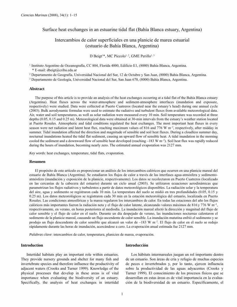
heat at a maximum rate after midday and loses it at a maximumrate near dawn (figs. 4, 5). Sensible heat flux showed two neg-ative maxima in summer and spring, the first in the morningand the second in the afternoon; however, only the second peakwas present during the rest of the year. Sensible heat flux wasnegative (downward direction) in each season, so air is trans-ferring heat to the tidal flat (sediment/water) throughout theentire year. This process seems to be more intense during thewarm seasons. The typical daily cycles of latent heat flux showthat maximum evaporation takes place during the hours ofmaximum insolation (figs. 4, 5). The higher summer andspring temperatures allow evaporation to develop even at nightwhen latent heat flux is reduced but still positive. During thecold seasons, however, latent heat flux is almost zero at night.Solar radiation heating of the tidal flat during the light hoursdetermines a positive value of advective flux (heat loss) duringthis period. The advective flux is reversed at night, when thecold surface of the tidal flat receives heat from winds and tides.

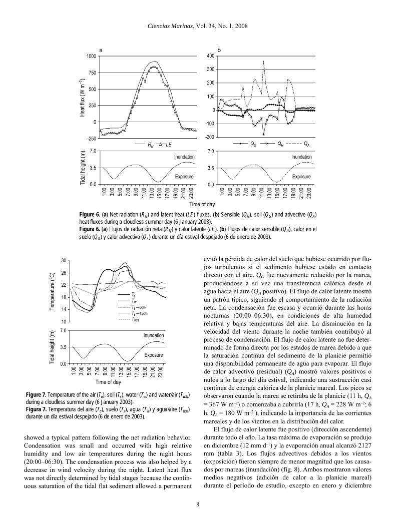
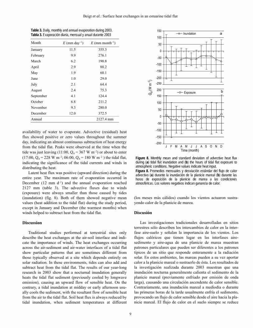
To study the heat-flux fluctuations due to the tide, severaldaily cycles were analyzed. The heat exchanges during acloudless summer day (6 January 2003) are shown as an exam-ple (fig. 6). The air, soil and water temperatures recorded on

negativos en verano y primavera; el primero durante la mañanay el segundo por la tarde. Sin embargo, sólo el segundo picoestá presente durante el resto del año. Puede observarse que elflujo de calor sensible es negativo (dirección descendente) entodas las estaciones del año, lo cual indica que el aire transfierecalor a la planicie de marea (sedimento/agua) a lo largo de todoel ciclo anual. Este proceso parece ser más intenso durante lasestaciones cálidas. Los ciclos diarios típicos de flujo de calorlatente muestran que la evaporación máxima tiene lugardurante las horas de máxima insolación (figs. 4, 5). Las mayo-res temperaturas del verano y primavera permiten que laevaporación se desarrolle incluso durante la noche, cuando LEse reduce pero aún es positivo. En tanto, durante las estacionesfrías el flujo de calor latente se acerca a cero en horas noctur-nas. El calentamiento de la planicie mareal por efecto de laradiación solar da un valor positivo al flujo advectivo (pérdidade calor) durante las horas de luz. La dirección de QA serevierte durante la noche, cuando la superficie fría de la plani-cie recibe calor de los vientos y las mareas.

Para estudiar las fluctuaciones de los flujos de calor debi-das a la marea, se analizaron diferentes ciclos diarios. Losintercambios calóricos ocurridos durante un día despejado de

Figure 4. Mean daily cycle of the heat fluxes in (a) summer and (b) spring 2003: RN = net radiation flux, LE = latentheat flux, QH = sensible heat flux, QG = soil heat flux, and QA = advective heat flux.Figura 4. Ciclo medio diario de los flujos de calor en (a) verano y (b) primavera de 2003: RN = flujo de radiación neta,LE = flujo de calor latente, QH = flujo de calor sensible, QG = flujo de calor en el suelo, y QA = flujo de calor advectivo.


7

that same day are shown in figure 7. During the first hoursof the day (00:00–06:30), the soil (heated by a previousinundation) was warmer than the air above it, allowing anupward flow of sensible and soil heat flux (figs. 6, 7). Thetidal flood of the morning (06:40–11:10) stopped the rapidheating of the sediment by solar radiation, holding the temper-ature at ~20.5ºC. Soil heat flux was soon reduced during thehours of inundation. Air transferred heat to water (negative QH)during this period. Sensible heat flux from air to soil was max-imum (–183 W m–2) when the tide was leaving the tidal flat andthe sediment was 4.1ºC colder than the air (fig. 7). During lowtide, the soil was heated by solar radiation, so an upward flowof sensible heat flux developed. Meanwhile, soil heat flux waspositive (downward direction), reaching 42 W m–2 at 13:40,when solar radiation and air temperature were highest. Beforethe next tide flooded the area (17:00–18:00, fig. 6), the air was1.7ºC warmer than the sediment below, so sensible heat fluxwas again negative (↓). At the same time, winds were subtract-ing heat from the tidal flat (positive QA). The second tidal floodprevented the soil heat loss that would have occurred by turbu-lent exchange if the sediment had been in contact with the air.Soil heat flux was again reduced by the tide, and a heat transferfrom water towards air (positive QH) occurred. Latent heat flux

verano (6 de enero de 2003) se muestran como ejemplo (fig. 6).Las temperaturas registradas en el aire, suelo y agua duranteese día se muestran en la figura 7. Durante las primeras horasdel día (00:00–06:30), el suelo (calentado por una inundaciónprevia) se hallaba más cálido que el aire por encima de él, per-mitiendo una circulación ascendente de QH y QG (figs. 6, 7). Lainundación mareal de la mañana (06:40–11:10) detuvo elrápido calentamiento del sedimento por radiación solar, mante-niendo su temperatura a ~20.5ºC. El flujo de calor en el suelo(QG) se redujo bruscamente durante las horas de inundación. Elaire transfirió calor al agua (QH negativo) durante este período.El flujo de calor sensible del aire hacia el suelo alcanzó sumáximo (–183 W m–2) cuando la marea se retiró de la planiciey el sedimento estaba 4.1ºC más frío que el aire (fig. 7).Durante la bajamar el suelo fue calentado por efecto de laradiación solar, desarrollándose un flujo ascendente de QH. Entanto, QG fue positivo (dirección descendente) alcanzando unvalor de 42 W m–2 a las 13:40, cuando la radiación solar y latemperatura del aire fueron máximas. Previamente a lasiguiente inundación (17–18 h, fig. 6), el aire estaba 1.7ºC máscálido que el sedimento, de manera que QH fue nuevamentenegativo (↓). Al mismo tiempo los vientos sustrajeron calor dela planicie mareal (QA positivo). La segunda inundación mareal

Figure 5. Mean daily cycle of the heat fluxes in (a) winter and (b) autumn 2003: RN = net radiation flux, LE = latent heatflux, QH = sensible heat flux, QG = soil heat flux, and QA = advective heat flux.Figura 5. Ciclo medio diario de los flujos de calor en (a) invierno y (b) otoño de 2003: RN = flujo de radiación neta,LE = flujo de calor latente, QH = flujo de calor sensible, QG = flujo de calor en el suelo, y QA = flujo de calor advectivo.


8

showed a typical pattern following the net radiation behavior.Condensation was small and occurred with high relativehumidity and low air temperatures during the night hours(20:00–06:30). The condensation process was also helped by adecrease in wind velocity during the night. Latent heat fluxwas not directly determined by tidal stages because the contin-uous saturation of the tidal flat sediment allowed a permanent

evitó la pérdida de calor del suelo que hubiese ocurrido por flu-jos turbulentos si el sedimento hubiese estado en contactodirecto con el aire. QG fue nuevamente reducido por la marea,produciéndose a su vez una transferencia calórica desde elagua hacia el aire (QH positivo). El flujo de calor latente mostróun patrón típico, siguiendo el comportamiento de la radiaciónneta. La condensación fue escasa y ocurrió durante las horasnocturnas (20:00–06:30), en condiciones de alta humedadrelativa y bajas temperaturas del aire. La disminución en lavelocidad del viento durante la noche también contribuyó alproceso de condensación. El flujo de calor latente no fue deter-minado de forma directa por los estados de marea debido a quela saturación contínua del sedimento de la planicie permitióuna disponibilidad permanente de agua para evaporar. El flujode calor advectivo (residual) (QA) mostró valores positivos onulos a lo largo del día estival, indicando una sustracción casicontínua de energía calórica de la planicie mareal. Los picos seobservaron cuando la marea se retiraba de la planicie (11 h, QA

= 367 W m–2) o comenzaba a cubrirla (17 h, QA = 228 W m–2; 6h, QA = 180 W m–2 ), indicando la importancia de las corrientesmareales y de los vientos en la distribución del calor.

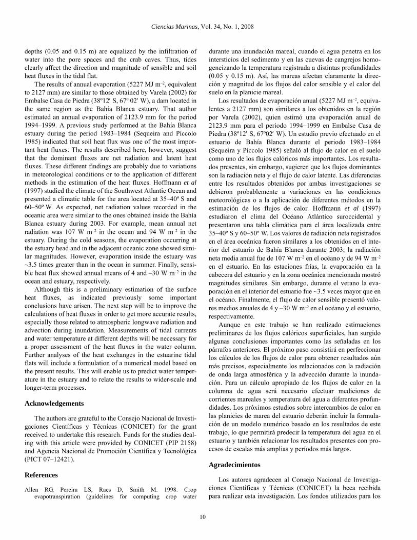
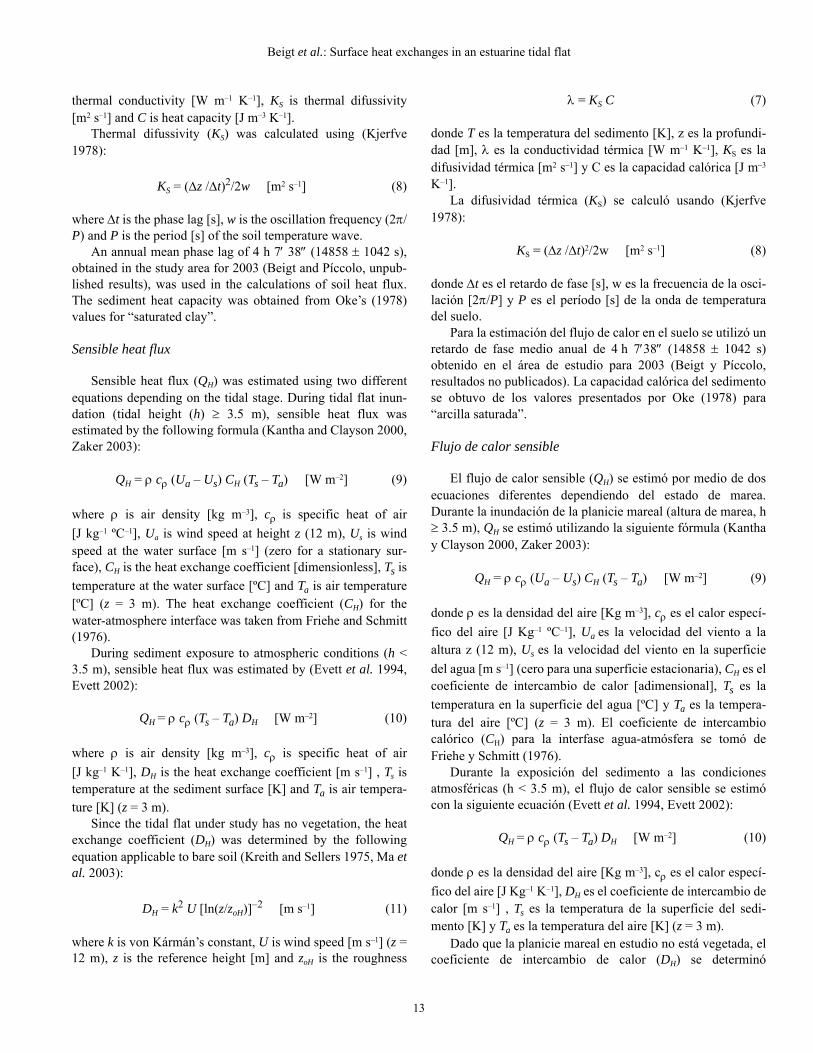
El flujo de calor latente fue positivo (dirección ascendente)durante todo el año. La tasa máxima de evaporación se produjoen diciembre (12 mm d–1) y la evaporación anual alcanzó 2127mm (tabla 3). Los flujos advectivos debidos a los vientos(exposición) fueron siempre de menor magnitud que los causa-dos por mareas (inundación) (fig. 8). Ambos mostraron valoresmedios negativos (adición de calor a la planicie mareal)durante el período de estudio, excepto en enero y diciembre

Figure 6. (a) Net radiation (RN) and latent heat (LE) fluxes. (b) Sensible (QH), soil (QG) and advective (QA)heat fluxes during a cloudless summer day (6 January 2003).Figura 6. (a) Flujos de radiación neta (RN) y calor latente (LE). (b) Flujos de calor sensible (QH), calor en elsuelo (QG) y calor advectivo (QA) durante un día estival despejado (6 de enero de 2003).

Figure 7. Temperature of the air (Ta), soil (Ts), water (Tw) and water/air (Tw/a)during a cloudless summer day (6 January 2003).Figura 7. Temperatura del aire (Ta), suelo (Ts), agua (Tw) y agua/aire (Tw/a)durante un día estival despejado (6 de enero de 2003).


9

availability of water to evaporate. Advective (residual) heatflux showed positive or zero values throughout the summerday, indicating an almost continuous subtraction of heat energyfrom the tidal flat. Peaks were observed at the time when thetide was just leaving (11:00, QA = 367 W m–2) or about to enter(17:00, QA = 228 W m–2; 06:00, QA = 180 W m–2 ) the tidal flat,indicating the significance of the tidal currents and winds indistributing the heat.

Latent heat flux was positive (upward direction) during theentire year. The maximum rate of evaporation occurred inDecember (12 mm d–1) and the annual evaporation reached2127 mm (table 3). The advective fluxes due to winds(exposure) were always smaller than those caused by tides(inundation) (fig. 8). Both of them showed negative meanvalues (heat addition to the tidal flat) during the study period,except in January and December (the warmest months) whenwinds helped to subtract heat from the tidal flat.

Discussion

Traditional studies performed at terrestrial sites onlydescribe the heat exchanges at the air-soil interface and indi-cate the importance of winds. The heat exchanges occurringacross the air-sediment and air-water interfaces of a tidal flatshow particular patterns that are sometimes different fromthose typically observed at a site which depends entirely onsolar radiation. In these environments, tides can also add andsubtract heat from the tidal flat. The results of our year-longresearch in 2003 show that a nocturnal inundation generallyheats the tidal flat sediment (previously cooled by longwaveemission), causing an upward flow of sensible heat. On thecontrary, a tidal inundation at midday or early afternoon usu-ally cools the sediment, with the resultant flow of sensible heatfrom the air to the tidal flat. Soil heat flux is always reduced bytidal inundation, when sediment temperatures at different

(los meses más cálidos) cuando los vientos actuaron sustra-yendo calor de la planicie de marea.

Discusión

Las investigaciones tradicionales desarrolladas en sitiosterrestres sólo describen los intercambios de calor en la inter-fase aire-suelo y señalan la importancia de los vientos. Losflujos calóricos que tienen lugar en las interfases aire-sedimento y aire-agua de una planicie de marea muestranpatrones particulares que pueden ser diferentes a los patronestípicos de un sitio que responde enteramente a la radiaciónsolar. En estos ambientes, las mareas pueden a su vez aportarcalor a la planicie mareal o sustraerlo de ésta. Los resultados dela investigación realizada durante 2003 muestran que unainundación nocturna generalmente calienta el sedimento de laplanicie mareal (previamente enfriado por emisión de ondalarga), causando una circulación ascendente de calor sensible.Contrariamente, una inundación mareal a mediodía o durantelas primeras horas de la tarde usualmente enfría el sedimento,provocando un flujo de calor sensible desde el aire hacia la pla-nicie mareal. El flujo de calor en el suelo siempre se reduce

Figure 8. Monthly mean and standard deviation of advective heat fluxduring (a) tidal flat inundation and (b) the hours of tidal flat exposure toatmospheric conditions. Negative values indicate heat input.Figura 8. Promedios mensuales y desviación estándar del flujo de caloradvectivo (a) durante la inundación de la planicie mareal (b) durante lashoras de exposición de la planicie de marea a las condicionesatmosféricas. Los valores negativos indican ganancia de calor.

Table 3. Daily, monthly and annual evaporation during 2003.Tabla 3. Evaporación diaria, mensual y anual durante 2003

Month E (mm day–1) E (mm month–1)

January 11.5 355.3February 9.9 276.1March 6.2 190.8April 2.9 88.2May 1.9 60.1June 1.0 29.0July 2.1 64.4August 2.4 75.3September 4.1 124.4October 6.8 211.2November 9.3 280.0December 12.0 372.5Annual 2127.4 mm


10

depths (0.05 and 0.15 m) are equalized by the infiltration ofwater into the pore spaces and the crab caves. Thus, tidesclearly affect the direction and magnitude of sensible and soilheat fluxes in the tidal flat.

The results of annual evaporation (5227 MJ m–2, equivalentto 2127 mm) are similar to those obtained by Varela (2002) forEmbalse Casa de Piedra (38º12′ S, 67º 02′ W), a dam located inthe same region as the Bahía Blanca estuary. That authorestimated an annual evaporation of 2123.9 mm for the period1994–1999. A previous study performed at the Bahía Blancaestuary during the period 1983–1984 (Sequeira and Píccolo1985) indicated that soil heat flux was one of the most impor-tant heat fluxes. The results described here, however, suggestthat the dominant fluxes are net radiation and latent heatfluxes. These different findings are probably due to variationsin meteorological conditions or to the application of differentmethods in the estimation of the heat fluxes. Hoffmann et al(1997) studied the climate of the Southwest Atlantic Ocean andpresented a climatic table for the area located at 35–40º S and60–50º W. As expected, net radiation values recorded in theoceanic area were similar to the ones obtained inside the BahíaBlanca estuary during 2003. For example, mean annual netradiation was 107 W m–2 in the ocean and 94 W m–2 in theestuary. During the cold seasons, the evaporation occurring atthe estuary head and in the adjacent oceanic zone showed simi-lar magnitudes. However, evaporation inside the estuary was~3.5 times greater than in the ocean in summer. Finally, sensi-ble heat flux showed annual means of 4 and –30 W m–2 in theocean and estuary, respectively.

Although this is a preliminary estimation of the surfaceheat fluxes, as indicated previously some importantconclusions have arisen. The next step will be to improve thecalculations of heat fluxes in order to get more accurate results,especially those related to atmospheric longwave radiation andadvection during inundation. Measurements of tidal currentsand water temperature at different depths will be necessary fora proper assessment of the heat fluxes in the water column.Further analyses of the heat exchanges in the estuarine tidalflats will include a formulation of a numerical model based onthe present results. This will enable us to predict water temper-ature in the estuary and to relate the results to wider-scale andlonger-term processes.

Acknowledgements

The authors are grateful to the Consejo Nacional de Investi-gaciones Científicas y Técnicas (CONICET) for the grantreceived to undertake this research. Funds for the studies deal-ing with this article were provided by CONICET (PIP 2158)and Agencia Nacional de Promoción Científica y Tecnológica(PICT 07–12421).

References

Allen RG, Pereira LS, Raes D, Smith M. 1998. Cropevapotranspiration (guidelines for computing crop water

durante una inundación mareal, cuando el agua penetra en losintersticios del sedimento y en las cuevas de cangrejos homo-geneizando la temperatura registrada a distintas profundidades(0.05 y 0.15 m). Así, las mareas afectan claramente la direc-ción y magnitud de los flujos del calor sensible y el calor delsuelo en la planicie mareal.

Los resultados de evaporación anual (5227 MJ m–2, equiva-lentes a 2127 mm) son similares a los obtenidos en la regiónpor Varela (2002), quien estimó una evaporación anual de2123.9 mm para el periodo 1994–1999 en Embalse Casa dePiedra (38º12′ S, 67º02′ W). Un estudio previo efectuado en elestuario de Bahía Blanca durante el periodo 1983–1984(Sequeira y Píccolo 1985) señaló al flujo de calor en el suelocomo uno de los flujos calóricos más importantes. Los resulta-dos presentes, sin embargo, sugieren que los flujos dominantesson la radiación neta y el flujo de calor latente. Las diferenciasentre los resultados obtenidos por ambas investigaciones sedebieron probablemente a variaciones en las condicionesmeteorológicas o a la aplicación de diferentes métodos en laestimación de los flujos de calor. Hoffmann et al (1997)estudiaron el clima del Océano Atlántico suroccidental ypresentaron una tabla climática para el área localizada entre35–40º S y 60–50º W. Los valores de radiación neta registradosen el área oceánica fueron similares a los obtenidos en el inte-rior del estuario de Bahía Blanca durante 2003; la radiaciónneta media anual fue de 107 W m–2 en el océano y de 94 W m–2

en el estuario. En las estaciones frías, la evaporación en lacabecera del estuario y en la zona oceánica mencionada mostrómagnitudes similares. Sin embargo, durante el verano la eva-poración en el interior del estuario fue ~3.5 veces mayor que enel océano. Finalmente, el flujo de calor sensible presentó valo-res medios anuales de 4 y –30 W m–2 en el océano y el estuario,respectivamente.

Aunque en este trabajo se han realizado estimacionespreliminares de los flujos calóricos superficiales, han surgidoalgunas conclusiones importantes como las señaladas en lospárrafos anteriores. El próximo paso consistirá en perfeccionarlos cálculos de los flujos de calor para obtener resultados aúnmás precisos, especialmente los relacionados con la radiaciónde onda larga atmosférica y la advección durante la inunda-ción. Para un cálculo apropiado de los flujos de calor en lacolumna de agua será necesario efectuar mediciones decorrientes mareales y temperatura del agua a diferentes profun-didades. Los próximos estudios sobre intercambios de calor enlas planicies de marea del estuario deberán incluir la formula-ción de un modelo numérico basado en los resultados de estetrabajo, lo que permitirá predecir la temperatura del agua en elestuario y también relacionar los resultados presentes con pro-cesos de escalas más amplias y períodos más largos.

Agradecimientos

Los autores agradecen al Consejo Nacional de Investiga-ciones Científicas y Técnicas (CONICET) la beca recibidapara realizar esta investigación. Los fondos utilizados para los


11

requirements). FAO Irrigation and Drainage Paper No. 56, Rome.Http://www.fao.org/docrep/X0490E/X0490E00.htm.

Beigt D, Piccolo MC, Perillo GME. 2003. Soil heat exchange inPuerto Cuatreros tidal flats, Argentina. Cienc. Mar. 29: 595–602.

Capelli de Steffens AM, Campo de Ferreras AM. 2004. Climatología.In: Píccolo MC, Hoffmeyer MS (eds.), Ecosistema del Estuario deBahía Blanca. Ed. Sapienza, Bahía Blanca, pp. 79–86.

Crooks S, Turner RK. 1999. Integrated coastal management:Sustaining estuarine natural resources. Adv. Ecol. Res. 29: 241–289.

Custodio E, Llamas MR. 1996. Hidrología Subterránea. Tomo I. Ed.Omega, Barcelona, 1157 pp.

de Laat PJM. 1996. Soil-water-plant relations. International Institutefor Infraestructural, Hydraulic and Environmental Engineering(IHE), Delft, Netherlands, 161 pp.

Evett SR. 2002. Water and energy balances at soil-plant-atmosphereinterfases. In: Warrick A (ed.), The Soil Physics Companion. CRCPress LLC, Florida, pp. 127–190.

Evett SR, Matthias AD, Warrick AW. 1994. Energy balance model ofspatially variable evaporation from bare soil. Soil Sci. Soc. Am. J.58: 1604–1611.

Freije RH, Asteasuain RO, Schmidt A, Zavatti JR. 1981. Relación dela salinidad y temperatura del agua con las condiciones hidro-meteorológicas en la porción interna del estuario de Bahía Blanca.Contribución Científica No. 57, IADO, Bahía Blanca, 20 pp.

Friehe CA, Schmitt KF. 1976. Parameterization of air-sea interfacefluxes of sensible heat and moisture by the bulk aerodynamicformulas. J. Phys. Oceanogr. 6: 801–809.

Harrison SJ, Phizacklea AP. 1985. Seasonal changes in heat flux andheat storage in the intertidal mudflats of the Forth Estuary,Scotland. J. Climatol. 5: 473–485.

Heath RA. 1976. Heat balance in a small coastal inlet. PauatahanuiInlet, North Island, New Zealand. Estuar. Coast. Mar. Sci. 5: 783–792.

Hoffmann JAJ, Núñez MN, Píccolo MC. 1997. Característicasclimáticas del Océano Atlántico Sudoccidental. Mar Argentino ysus Recursos Pesqueros 1: 163–193.

Hollins S, Ridd PV. 1997. Evaporation over a tropical tidal salt flat.Mangroves Salt Marshes 1: 95–102.

Hsu SA. 1978. Micrometeorological fluxes in estuaries. In: Hsu SA(ed.), Estuarine Transport Processes. The Belle Baruch Library inMarine Sciences No. 7. Univ. South Carolina Press, Columbia,pp. 125–134.

Hughes CE, Kalma JD, Binning P, Willgoose GR, Vertzonis M. 2001.Estimating evapotranspiration for a temperate salt marsh,Newcastle, Australia. Hydrol. Proc. 15: 957–975.

Kantha LH, Clayson CA. 2000. Small-scale Processes in GeophysicalFluid Flows. International Geophysics Ser. Vol. 67. AcademicPress, USA, 888 pp.

Kjerfve B. 1978. Diurnal energy balance of a Caribbean barrier reefenvironment. Bull. Mar. Sci. 28: 137–145.

Kreith F, Sellers WD. 1975. General principles of natural evaporation.In: de Vries DA, Afgan NH (eds.), Heat and Mass Transfer in theBiosphere. Part 1. John Wiley and Sons, New York, pp. 207–227.

Ma Y, Su Z, Koike T, Yao T, Ishikawa H, Ueno K, Menenti M. 2003.On measuring and remote sensing surface energy partitioningover the Tibetan Plateau, from GAME/Tibet to CAMP/Tibet.Phys. Chem. Earth 28: 63–74.

estudios concernientes a este artículo han sido provistos por elCONICET (PIP 2158) y por la Agencia Nacional de Promo-ción Científica y Tecnológica (ANPCYT) (PICT 07–12421).

Mailhot J, Bélair S, Benoit R, Bilodeau B, Delage Y, Fillion L, GarandL, Girard C, Tremblay A. 1998. Scientific Description of RPNPhysics Library. Ed. Recherche en Prévision Numérique,Meteorological Service of Canada, Dorval, Québec, 188 pp.

Monteith JL. 1973. Principles of Environmental Physics. EdwardArnold Publisher, London.

Odum EP. 1975. Ecology. 2nd ed. Holt, Rinehart and Winston, NewYork, 639 pp.

Oke TR. 1978. Boundary Layer Climates. Methuen, London, 372 pp.Perillo GME, Píccolo MC. 1991. Tidal response in the Bahía Blanca

estuary, Argentina. J. Coast. Res. 7: 447–449.Perillo GME, Píccolo MC, Parodi E, Freije RH. 2000. The Bahía

Blanca estuary, Argentina. In: Seeliger U, Kjerfve B (eds.),Coastal Marine Ecosystems of Latin America: Ecological Studies.Vol. 144. Springer-Verlag, Berlin, pp. 205–217.

Perillo GME, Píccolo MC, Palma E, Pérez DE, Pierini J. 2004.Oceanografía Física. In: Píccolo MC, Hoffmeyer MS (eds.),Ecosistema del Estuario de Bahía Blanca. Instituto Argentino deOceanografía, Bahía Blanca, pp. 61–67.

Remenieras G. 1960. L’Hydrologie de l’Ingénieur. Eyrolles Editeur,Paris, 316 pp.

Sequeira ME, Píccolo MC. 1985. Predicción de la temperatura delagua durante la bajante de la marea en Ingeniero White.Meteorologica 15: 59–76.

Serman D, Cardini J. 1983. Predicción de la temperatura del agua enla ría interior de Bahía Blanca. Acta Oceanogr. Argentina 3(2).

Smith NP. 1977. A note on winter temperature variations in a shallowseagrass flat. Limnol. Oceanogr. 22: 1079–1082.

Smith NP. 1981. Energy balance in a shallow seagrass flat for winterconditions. Limnol. Oceanogr. 26: 482–491.

Smith NP, Kierspe GH. 1981. Local energy exchanges in a shallowcoastal lagoon: Winter conditions. Estuar. Coast. Shelf Sci. 13:159–167.

Swinbank WC. 1963. Long-wave radiation from clear skies. R.Meteorol. Soc. 89: 339–348.

van Wijk WR, Scholte Ubing DW. 1963. Radiation. In: van Wijk WR(ed.), Physics of Plant Environment. North Holland PublicationsCo., Amsterdam, pp. 62–101.

Varela PA. 2002. Estudio de evaporación del Embalse Casa de Piedra.Río Colorado, La Pampa–Río Negro. Tech. Rep. METEOSURAsesoramiento Meteorológico, Bahía Blanca, 11 pp.

Vugts HF, Zimmerman JTF. 1985. The heat balance of a tidal flat area.Neth. J. Sea Res. 19: 1–14.

Wallace JS, Holwill CJ. 1997. Soil evaporation from tiger-bush insouth-west Niger. J. Hydrol. 188–189: 426–442.

Zaker NH. 2003. Computation and modeling of the air-sea heat andmomentum fluxes. Ed. International Centre for TheoreticalPhysics, Italy, 9 pp.

Recibido en diciembre de 2006;aceptado en octubre de 2007.


12

Appendix

Net radiation

Different bulk aerodynamic formulas were used to estimatethe radiative and turbulent fluxes from available meteorologi-cal data. Net radiation (RN) was determined from incident solarradiation and temperature data using (Evett 2002):

RN = Rsi (1 – α) – L↑ + L↓ (2)

where Rsi is incident solar radiation [W m–2], α is albedo, L↑ isterrestrial longwave radiation from water and soil [W m–2] andL↓ is atmospheric longwave radiation [W m–2].

Terrestrial longwave radiation (L↑) was estimated by thefollowing equation (Evett 2002):

L↑ = ∈s σ Ts4 (3)

where ∈s is surface emissivity, σ is Stefan-Boltzmann’s con-stant [W m–2 K–4] and Ts is surface temperature [K] (water orsediment temperature, depending on tidal stage).

Atmospheric longwave radiation (L↓) was estimated usingtwo different equations depending on the temperature data.Equation 4 (Swinbank 1963) was used when air temperaturewas higher than 0ºC, whereas equation 5 (Monteith 1973) wasused for temperatures lower than 0ºC and higher than –5ºC.

L↓ = 1.20 σ Ta4 – 171 (4)

where σ is Stefan-Boltzmann’s constant and Ta is air tempera-ture [K],

L↓ = 208 + 6 Ta (5)

where Ta is air temperature [ºC].As previously mentioned, due to the complexity of a tidal

flat environment, some assumptions (i.e., cloudless conditionsover the study period) were made in order to simplify the cal-culations. Surface emissivity and albedo of thetidal flat wereobtained from tables (van Wijk and Scholte Ubing 1963, deLaat 1996, Kantha and Clayson 2000).

Soil heat flux

Soil heat flux (QG) across the surface layer (0.05–0.15 mdepth) was determined from temperature data using the Fourierequation (Oke 1978):

QG = –λ (ΔT/Δz) [W m–2] (6)

λ = KS C (7)

where T is sediment temperature [K], z is depth (m), λ is

Apéndice

Radiación neta

Se utilizaron diferentes fórmulas aerodinámicas de masapara estimar los flujos radiativos y turbulentos a partir de losdatos meteorológicos disponibles. La radiación neta (RN) sedeterminó a partir de la radiación solar incidente y la tempera-tura usando (Evett 2002):

RN = Rsi (1 – α) – L↑ + L↓ (2)

donde Rsi es la radiación solar incidente [W m–2], α es elalbedo, L↑ es la radiación de onda larga terrestre (agua/sedi-mento) [W m–2] y L↓ es la radiación de onda larga atmosférica[W m–2].

La radiación de onda larga terrestre (L↑) se estimó a partirde la siguiente ecuación (Evett 2002):

L↑ = ∈s σ Ts 4 (3)

donde ∈s es la emisividad de la superficie, σ es la constanteStefan-Boltzmann [W m–2 K–4] y Ts es la temperatura de lasuperficie [K] (temperatura del agua o el sedimento, depen-diendo del estado de marea).

La radiación de onda larga atmosférica (L↓) se estimóusando dos ecuaciones distintas según los datos de tempera-tura. La ecuación 4 (Swinbank 1963) se utilizó cuando latemperatura del aire fue superior a 0ºC y la ecuación 5(Monteith, 1973) se aplicó a temperaturas inferiores a 0ºC ysuperiores a –5ºC.

L↓ = 1.20 σ Ta4 – 171 (4)

donde σ es la constante Stefan-Boltzmann y Ta es la tempera-tura del aire [K].

L↓ = 208 + 6 Ta (5)

donde Ta es la temperatura del aire [ºC].Como se mencionó previamente, debido a la complejidad

del ambiente intermareal, se realizaron algunas suposiciones(por ejemplo, condiciones de cielo despejado durante elperíodo de estudio) con el objeto de simplificar los cálculos. Laemisividad de la superficie y el albedo de la planicie mareal seobtuvieron de tablas (van Wijk y Scholte Ubing 1963, de Laat1996, Kantha y Clayson 2000).

Flujo de calor en el suelo

El flujo de calor en el suelo (QG) a través de la capa superfi-cial (0.05–0.15 m de profundidad) se determinó en base a datosde temperatura utilizando la ecuación de Fourier (Oke 1978):

QG = –λ (ΔT/Δz) [W m–2] (6)


13

thermal conductivity [W m–1 K–1], KS is thermal difussivity[m2 s–1] and C is heat capacity [J m–3 K–1].

Thermal difussivity (KS) was calculated using (Kjerfve1978):

KS = (Δz /Δt)2/2w [m2 s–1] (8)

where Δt is the phase lag [s], w is the oscillation frequency (2π/P) and P is the period [s] of the soil temperature wave.

An annual mean phase lag of 4 h 7′ 38″ (14858 ± 1042 s),obtained in the study area for 2003 (Beigt and Píccolo, unpub-lished results), was used in the calculations of soil heat flux.The sediment heat capacity was obtained from Oke’s (1978)values for “saturated clay”.

Sensible heat flux

Sensible heat flux (QH) was estimated using two differentequations depending on the tidal stage. During tidal flat inun-dation (tidal height (h) ≥ 3.5 m), sensible heat flux wasestimated by the following formula (Kantha and Clayson 2000,Zaker 2003):

QH = ρ cρ (Ua – Us) CH (Ts – Ta) [W m–2] (9)

where ρ is air density [kg m–3], cρ is specific heat of air[J kg–1 ºC–1], Ua is wind speed at height z (12 m), Us is windspeed at the water surface [m s–1] (zero for a stationary sur-face), CH is the heat exchange coefficient [dimensionless], Ts istemperature at the water surface [ºC] and Ta is air temperature[ºC] (z = 3 m). The heat exchange coefficient (CH) for thewater-atmosphere interface was taken from Friehe and Schmitt(1976).

During sediment exposure to atmospheric conditions (h <3.5 m), sensible heat flux was estimated by (Evett et al. 1994,Evett 2002):

QH = ρ cρ (Ts – Ta) DH [W m–2] (10)

where ρ is air density [kg m–3], cρ is specific heat of air[J kg–1 K–1], DH is the heat exchange coefficient [m s–1] , Ts istemperature at the sediment surface [K] and Ta is air tempera-ture [K] (z = 3 m).

Since the tidal flat under study has no vegetation, the heatexchange coefficient (DH) was determined by the followingequation applicable to bare soil (Kreith and Sellers 1975, Ma etal. 2003):

DH = k2 U [ln(z/zoH)]–2 [m s–1] (11)

where k is von Kármán’s constant, U is wind speed [m s–1] (z =12 m), z is the reference height [m] and zoH is the roughness

λ = KS C (7)

donde T es la temperatura del sedimento [K], z es la profundi-dad [m], λ es la conductividad térmica [W m–1 K–1], KS es ladifusividad térmica [m2 s–1] y C es la capacidad calórica [J m–3

K–1]. La difusividad térmica (KS) se calculó usando (Kjerfve

1978):

KS = (Δz /Δt)2/2w [m2 s–1] (8)

donde Δt es el retardo de fase [s], w es la frecuencia de la osci-lación [2π/P] y P es el período [s] de la onda de temperaturadel suelo.

Para la estimación del flujo de calor en el suelo se utilizó unretardo de fase medio anual de 4 h 7′38″ (14858 ± 1042 s)obtenido en el área de estudio para 2003 (Beigt y Píccolo,resultados no publicados). La capacidad calórica del sedimentose obtuvo de los valores presentados por Oke (1978) para“arcilla saturada”.

Flujo de calor sensible

El flujo de calor sensible (QH) se estimó por medio de dosecuaciones diferentes dependiendo del estado de marea.Durante la inundación de la planicie mareal (altura de marea, h≥ 3.5 m), QH se estimó utilizando la siguiente fórmula (Kanthay Clayson 2000, Zaker 2003):

QH = ρ cρ (Ua – Us) CH (Ts – Ta) [W m–2] (9)

donde ρ es la densidad del aire [Kg m–3], cρ es el calor especí-fico del aire [J Kg–1 ºC–1], Ua es la velocidad del viento a laaltura z (12 m), Us es la velocidad del viento en la superficiedel agua [m s–1] (cero para una superficie estacionaria), CH es elcoeficiente de intercambio de calor [adimensional], Ts es latemperatura en la superficie del agua [ºC] y Ta es la tempera-tura del aire [ºC] (z = 3 m). El coeficiente de intercambiocalórico (CH) para la interfase agua-atmósfera se tomó deFriehe y Schmitt (1976).

Durante la exposición del sedimento a las condicionesatmosféricas (h < 3.5 m), el flujo de calor sensible se estimócon la siguiente ecuación (Evett et al. 1994, Evett 2002):

QH = ρ cρ (Ts – Ta) DH [W m–2] (10)

donde ρ es la densidad del aire [Kg m–3], cρ es el calor especí-fico del aire [J Kg–1 K–1], DH es el coeficiente de intercambio decalor [m s–1] , Ts es la temperatura de la superficie del sedi-mento [K] y Ta es la temperatura del aire [K] (z = 3 m).

Dado que la planicie mareal en estudio no está vegetada, elcoeficiente de intercambio de calor (DH) se determinó


14

length for sensible heat flux [m]. The roughness length (zoH) fora bare soil was taken from Kreith and Sellers (1975).

Latent heat flux

Latent heat flux (LE) across the sediment-atmosphere andwater-atmosphere interfaces was estimated by the Penman-Monteith equation (12). Although it is usually applied inagronomy studies of vegetated and bare soils, it has also beenapplied to salt marshes (Hughes et al. 2001) and tidal flats(Harrison and Phizacklea 1985). The result of the Penman-Monteith equation is the “potential evaporation rate”, i.e., theevaporation rate that occurs when water availability is notlimiting. Taking into account that the sediments of the studiedtidal flat are permanently saturated, assessing the potentialevaporation was considered correct.

As mentioned, the Penman-Monteith equation was appliednot only to the sediment-atmosphere interface but also to thewater-atmosphere interface. This decision was based on thefact that evaporation from a saturated soil is nearly the same asevaporation from a free water surface having the same environ-mental conditions (Custodio and Llamas 1996). For example,the evaporation occurring on saturated fine sand is equivalentto that occurring on a free water surface, while the evaporationon saturated clay represents 75–85% of the evaporation on afree water surface (Remenieras 1960). The Penman-Monteithequation is expressed as:

[MW m–2] (12)

where Δ is the slope of the saturation vapour pressure vs tem-perature relationship [kPa ºC–1], ρ is air density [kg m–3], cρ isspecific heat of air [MJ kg–1 ºC–1], (es – ea) represents thevapour pressure deficit of the air [kPa] (z = 3 m), ra is aerody-namic resistance [s m–1], rs is surface resistance [s m–1] and γ isthe psychrometric constant [kPa ºC–1].

When the soil is bare, rs = 0; thus, the previous equation issummarized as follows (Wallace and Holwill 1997):

[MW m–2] (13)

The value of Δ was calculated by the following equation(Allen et al. 1998):

[kPa ºC–1] (14)

where Ta is air temperature [ºC].

LEΔ RN QG–( ) ρcρ es ea–( ) ra⁄+

Δ γ 1 rs ra⁄+( )+---------------------------------------------------------------------------=


Δ γ+---------------------------------------------------------------------------=

Δ4098 0.6108 17.27Ta( ) Ta 237.3+( )⁄[ ]exp{ }

Ta 237.3+( )2-------------------------------------------------------------------------------------------------------=

mediante una fórmula aplicable a suelo desnudo (Kreith ySellers 1975, Ma et al. 2003):

DH = k2 U [ln(z/zoH)]–2 [m s–1] (11)

donde k es la constante de von Kármán, U es la velocidad delviento [m s–1] (z = 12 m), z es la altura de referencia [m] y zoH

es la longitud de rugosidad para flujo de calor sensible [m]. Lalongitud de rugosidad (zoH) para un suelo desnudo se tomó deKreith y Sellers (1975).

Flujo de calor latente

El flujo de calor latente (LE) a través de las interfasessedimento-atmósfera y agua-atmósfera se estimó mediante laecuación de Penman-Monteith (12). Si bien ésta es una ecua-ción ampliamente utilizada en estudios agronómicos de suelosvegetados y desnudos, también ha sido aplicada en marismassaladas (Hughes et al. 2001) y planicies de marea (Harrison yPhizacklea 1985). La ecuación Penman-Monteith da comoresultado la “tasa de evaporación potencial”, es decir, aquéllaque se produce en un suelo donde la disponibilidad de agua noes limitante. Teniendo en cuenta que los sedimentos de la pla-nicie mareal estudiada se hallan permanentemente saturados,se consideró correcto estimar la evaporación potencial.

Como se mencionó previamente, la ecuación de Penman-Monteith se aplicó no sólo a la interfase sedimento-atmósferasino también a la interfase agua-atmósfera. Se tomó esta deci-sión dado que la evaporación desde un suelo saturado tiene unvalor cercano al de una superficie de agua libre en las mismascondiciones ambientales (Custodio y Llamas 1996). Por ejem-plo, la evaporación que se produce en arenas finas saturadas esequivalente a la que tiene lugar en una superficie de agua libre,mientras que la evaporación en arcillas saturadas representa el75–85% de la evaporación en una superficie de agua libre(Remenieras 1960). La ecuación de Penman-Monteith seexpresa de la siguiente manera:

[MW m–2] (12)

donde Δ es la pendiente de la curva temperatura vs. presión devapor de saturación [kPa ºC–1], ρ es densidad del aire [Kg m–3],cρ es el calor específico del aire [MJ Kg–1 ºC–1], (es – ea) repre-senta el déficit de presión de vapor del aire [kPa] (z = 3 m), ra

es la resistencia aerodinámica [s m–1], rs es la resistencia super-ficial [s m–1] y γ es la constante psicrométrica [kPa ºC–1].

Para el caso de un suelo desnudo, rs = 0, por lo tanto laecuación previa puede resumirse como sigue (Wallace yHolwill 1997):

[MW m–2] (13)


Δ γ 1 rs ra⁄+( )+---------------------------------------------------------------------------=


Δ γ+---------------------------------------------------------------------------=


15

The vapour pressure deficit was obtained from (Allen et al.1998, Evett 2002):

[kPa] (15)

[kPa] (16)

where RH is the relative humidity [%]Aerodynamic resistance was estimated for neutral atmo-

spheric conditions from (Allen et al. 1998, Evett 2002):

[s m–1] (17)

where z is the height of wind speed measurements [m] (12 m),d is the zero plane displacement height [m], zoM is the rough-ness length governing momentum transfer [m], zH is the heightof air temperature and relative humidity measurements [m], zoH

is the roughness length governing sensible heat transfer [m], kis von Kármán’s constant and U is wind speed [m]. The valuesof zoH and zoM for a bare soil were taken from tables (Kreith andSellers 1975, Mailhot et al. 1998), while d is equal to zero for abare soil (Kreith and Sellers 1975).

Advective heat flux

The horizontal transport of heat or “advection” causes theaddition (or subtraction) of energy to (from) a tidal flat. Themost common agent of this process is wind; however, tide mustalso be considered when studying a tidal flat. Tidal energy gen-erally acts as an “energy subsidy” to the coastal ecosystem(Odum 1975). In this paper advective heat flux (QA) was esti-mated as the residual energy from the heat budget equation(18). The total advective flux was then divided according to thetidal height into two different fluxes: advective flux at expo-sure and advective flux at inundation. The first is carried bywinds, while tide is considered to be the main agent duringinundation.

QA = RN – QG – QH – LE [W m–2] (18)

ea RH * es( ) 100⁄=

es 0.6108 17.27Ta( ) Ta 237.3+( )⁄exp[ ]=

raz d–( ) zoM⁄[ ] zH d–( ) zoH⁄[ ]lnln

k2U---------------------------------------------------------------------------------=

El valor de Δ se calculó mediante la siguiente ecuación(Allen et al. 1998):

[kPa ºC–1] (14)

donde Ta es la temperatura del aire [ºC]El déficit de presión de vapor se obtuvo de las siguientes

fórmulas (Allen et al. 1998, Evett 2002):

[kPa] (15)

[kPa] (16)

donde RH es humedad relativa [%]La resistencia aerodinámica se estimó para condiciones de

estabilidad neutra (Allen et al. 1998, Evett 2002):

[s m–1] (17)

donde z es la altura de medición de la velocidad del viento [m](12 m), d es la altura de desplazamiento del plano cero [m], zoM

es la longitud de rugosidad para la cantidad de movimiento[m], zH es la altura de medición de la temperatura del aire yhumedad relativa [m], zoH es la longitud de rugosidad paratransporte de calor sensible [m], k es la constante de vonKármán y U es la velocidad del viento [m]. Los valores de zoH yzoM para un suelo desnudo se tomaron de tablas (Kreith ySellers 1975, Mailhot et al. 1998). Cabe hacer notar que d equi-vale a cero para el caso de un suelo desnudo (Kreith y Sellers1975).

Flujo de calor advectivo

El transporte horizontal de calor o “advección” causa laadición o sustracción de energía a o de la planicie mareal. Elagente más común de este proceso es el viento; sin embargo,cuando se estudia una planicie mareal también debe ser consi-derada la marea. La energía de las mareas generalmente actúacomo un “subsidio” de energía al ecosistema costero (Odum1975). En este trabajo el flujo de calor advectivo (QA) se estimócomo la energía residual de la ecuación de balance de calor(18). El flujo advectivo total luego se discriminó de acuerdo ala altura de marea en dos flujos diferentes (“flujo advectivo deexposición” y “flujo advectivo de inundación”). El primero estransportado por los vientos, mientras que la marea es conside-rada el principal agente durante la inundación.

QA = RN – QG – QH – LE [W m–2] (18)

Δ4098 0.6108 17.27Ta( ) Ta 237.3+( )⁄[ ]exp{ }

Ta 237.3+( )2-------------------------------------------------------------------------------------------------------=

ea RH * es( ) 100⁄=

es 0.6108 17.27Ta( ) Ta 237.3+( )⁄exp[ ]=

raz d–( ) zoM⁄[ ] zH d–( ) zoH⁄[ ]lnln

k2U---------------------------------------------------------------------------------=

Documents

Surface heat exchanges in an estuarine tidal flat (Bahía ...klinck/Reprints/PDF/beigtCienMar2008.pdf · Resumen El propósito de este artículo es proporcionar un análisis de los