Embed Size (px)
Citation preview
Surface Extraction and Flattening for Anatomical Visualization
Thèse n° 3575 (2006)
PRESENTEE A LA FACULTE INFORMATIQUE & COMMUNICATIONS
ECOLE POLYTECHNIQUE FEDERALE DE LAUSANNE
POUR L’OBTENTION DU GRADE DE DOCTEUR ES SCIENCES
PAR
LAURENT SAROUL
Ingénieur en électronique CPE-Lyon, DEA de Traitement de l’Image, Université de Saint-Etienne, France de nationalité française
Prof. W. Gerstner, président du jury Prof. R.D. Hersch, directeur de thèse
Prof. Eduard Gröller, rapporteur Dr. Jean Marie Becker, rapporteur
Dr. Ronan Boulic, rapporteur
Lausanne, EPFL 2006

2
3
Table of Contents
Table of Contents...................................................................................................3
Acknowledgements ...............................................................................................7
Abstract..................................................................................................................9
Résumé ................................................................................................................11
Notations..............................................................................................................13
1 Introduction.......................................................................................................15
1.1 Preface......................................................................................................................................... 15
1.2 Previous research on visualization of volume images ................................................................ 15
1.3 Contents of this work .................................................................................................................. 18
1.4 The Visible Human dataset ......................................................................................................... 20
2 Fundamental notions on curves, surfaces and differential geometry ...............21
2.1 Curves ......................................................................................................................................... 21
2.2 Parametric surfaces ..................................................................................................................... 22
2.3 Geodesic and normal curvature of a surface curve ..................................................................... 23
2.3.1 Definitions .......................................................................................................................................... 23
2.3.2 Calculation of principal curvatures..................................................................................................... 26
3 Curved surface extraction for exploring anatomic structures ..........................27
3.1 Previous work on curved surface extraction ............................................................................... 27
3.2 Ruled surface extraction from 3D volume images...................................................................... 28
3.2.1 Specification and extraction of a ruled surface ................................................................................... 28
3.2.2 Flattening of a ruled surface for visualization .................................................................................... 31
3.3 Free-form surface extraction from 3D volume images ............................................................... 33
3.3.1 Specification and extraction of free-form surfaces ............................................................................. 33
3.3.3 Visualizing free-form textured surfaces using a flattened view.......................................................... 37
3.4 Interactive specification of surfaces............................................................................................ 38
3.5 Exploration of anatomic structures with surfaces and 3D models .............................................. 40
3.6 Conclusion .................................................................................................................................. 42
4 Introduction to surface flattening .....................................................................43
4.1 Introduction................................................................................................................................. 43
4.2 Surface parameterization concept ............................................................................................... 44
4
4.2.1 Mapping definition ............................................................................................................................. 44
4.2.2 Isometric, conformal, harmonic and equiareal mappings ................................................................... 44
4.2.3 Definitions of surface parameterization, surface flattening and texture mapping............................... 45
4.2.4 Cartographic projections.................................................................................................................... 48
4.3 Previous work on surface parameterization ................................................................................ 49
4.4 Bennis et. al. Algorithm and Geodesic Curvature preservation.................................................. 51
4.4.1 Outline of the approach ...................................................................................................................... 51
4.4.2 Curve flattening with arc length and geodesic curvature preservation ............................................... 52
4.4.3 Bennis et. al. Algorithm...................................................................................................................... 53
4.6 Conclusion .................................................................................................................................. 55
5 Distance preserving flattening of surface sections: parallel planes and radial planes flattening...................................................................................................57
5.1 Introduction................................................................................................................................. 57
5.2 Parallel planes flattening............................................................................................................. 58
5.3 Radial planes flattening............................................................................................................... 60
5.4 Evaluation of the flattening methods by distortion measurements ............................................. 62
5.5 Interactive Flattening .................................................................................................................. 69
5.6 Carrying out measurements along flattened surfaces.................................................................. 72
5.7 Conclusion .................................................................................................................................. 74
6 Optimal parallel planes flattening ....................................................................77
6.1 Introduction................................................................................................................................. 77
6.2 Optimal plane orientation minimizing the geodesic curvature ................................................... 78
6.3 Minimizing the overall geodesic curvature by principal component analysis ............................ 80
6.4 Optimal parallel planes flattening of curved surfaces................................................................. 82
6.4.1 Distortions of optimally flattened surfaces ......................................................................................... 82
6.4.2 Comparison with Bennis et. al. surface flattening .............................................................................. 87
6.4.3 Computation times.............................................................................................................................. 90
6.5 Flattening of anatomical surfaces ............................................................................................... 90
6.6 Conclusion .................................................................................................................................. 94
7 Integration of surface extraction and flattening into the Visible Human server project ..................................................................................................................95
7.1 Introduction................................................................................................................................. 95
7.2 The Visible Human Server project.............................................................................................. 96
7.2.1 Previous works ................................................................................................................................... 96
7.2.2 History ................................................................................................................................................ 96
7.2.3 Visible Human server framework....................................................................................................... 98
7.3 Surface texture extraction ......................................................................................................... 100

5
7.3.1 Basic principles................................................................................................................................. 100
7.3.2 Slice extraction ................................................................................................................................. 101
7.3.3 Ruled surface texture extraction ....................................................................................................... 102
7.3.4 Curved surface texture extraction ..................................................................................................... 103
7.4 Java applet functionalities......................................................................................................... 106
7.4.1 Curved surface flattening.................................................................................................................. 106
7.4.2 Interactive rotation of the distance-preservation orientation ............................................................ 107
7.4.3 Specification of a region of interest for parallel planes flattening .................................................... 108
7.4.4 Measurements on flattened surfaces ................................................................................................. 109
7.5 Conclusion ................................................................................................................................ 109
8 Conclusion ......................................................................................................111
Appendices ........................................................................................................115
A. Cubic spline interpolation .......................................................................................................... 115
B. Glossary of medical terms.......................................................................................................... 117
C. Java applet user interface ........................................................................................................... 120
References..........................................................................................................129
Biography ..........................................................................................................135

6

7
Acknowledgements
First of all, I would like to thank Professor Roger David Hersch for giving me the opportunity to complete this work at the Peripheral Systems Laboratory (LSP) of the EPFL under his direction. His continuous guidance, his interesting remarks and advice helped me to reach the objectives of this work.
I also would like to thank Oscar Figueiredo from CPE-Lyon (France) which helped me to carry out this research.
I would like to give special thanks to Jean-Marie Becker from CPE-Lyon for his precious help for solving several mathematical problems encountered during this work, to Sebastian Gerlach who helped me in the development of the software presented in this work, to Isaac Amidror who helped me to improve the English of this thesis, and to all the persons who contributed to the project, especially Prof. J.P. Hornung and Dr B. Riederer, from the University of Lausanne, faculty of medicine and Lionel Micol, student from the University of Lausanne, faculty of medicine.
I also would like to thank all the LSP staff, especially Sylvain Chosson and Fabienne Allaire.
Finally, special thanks to my family and friends, for their help and support during these years.

8
9
Abstract
In the last years, three-dimensional (3D) medical imaging techniques have taken an increasing importance in patient care and medical research. Volume images provide medical specialists with a direct access to the interior of a patient’s body and reduce the need for invasive exploration. The use of volume imaging modalities such as X-ray CT, PET or MRI has therefore become essential for medical diagnosis and surgical planning.
Computer visualization techniques such as extraction of planar slices of arbitrary orientation (Multiplanar Reprojection), surface rendering of anatomic structures, and volume rendering provide medical users with the tools for exploiting 3D volume images.
Surface or respectively volume rendering provides information about the 3D geometry and 3D context of the structures of interest but does not allow to directly visualize original intensities, respectively colors located within the 3D structures. In addition, surface rendering requires the segmentation of the volume data and volume rendering often requires a classification of the volume image pixels. In contrast, the extraction of planar sections provides interactivity, requires no pre-processing and the original intensity, respectively color of each slice element may be directly inspected. However, it does not allow the visualization of curved anatomic structures within a single slice. In this thesis, we propose to overcome this limitation by generalizing the concept of planar section to the extraction of curved cross-sections.
In the first part, we focus on the interactive extraction of curved surfaces from volume images. Unlike planar slices, curved cross-sections may follow the trajectory of tubular structures such as the Aorta or follow structures with an irregular shape such as the Pelvis. In the second part of this work, we focus on the visualization of curved surfaces. We would like to offer the possibility of carrying out distance measurements along a structure of interest both for medical applications and for anatomical studies. Orthogonal or perspective projection of curved surfaces induces angular and metric distortions as well as surface overlapping. In order to enable measurements, we propose to use surface flattening methods, which preserve distances along specific orientations and minimize distortions around a focus point. Flattening of curved cross-sections enables inspecting spatially complex relationship between anatomic structures and their neighbourhood. They also allow the visualization of a curved anatomic structure within a single planar view and therefore to precisely inspect the original intensity, respectively color at each surface point. Thanks to a multi-resolution approach, surfaces are flattened at interactive rates, allowing users to displace the focus point during the visualization of the flattened surface. We also propose a new efficient method for computing a flattened surface minimizing global distortions and still preserving distances along one orientation.
Surface extraction and flattening techniques are integrated into an interactive visualization Java applet. This Java applet enables anyone to precisely and interactively inspect the Visible Human anatomy. Besides medical visualization, the presented methods may also be useful for creating new interesting views of anatomic structures for didactic purposes.

10
Keywords: medical visualization, anatomic structures, texture extraction, curved sections, free-form surfaces, surface flattening, differential geometry.
11
Résumé
Ces dernières années, les techniques d’imagerie médicale tridimensionnelles (3D) ont prit de plus en plus d’importance dans les domaines du traitement et de la recherche médicale. Les images volumiques fournissent aux spécialistes en médecine un accès direct à l’intérieur du corps d’un patient ce qui réduit le recours à des explorations invasives. L’utilisation des procédés d’acquisition d’images volumiques comme l’Imagerie à Résonance Magnétique (IRM), la tomographie à rayon X ou la Tomographie à Emission de Positrons (TEP), est donc devenue essentielle pour le diagnostic ou la planification d’intervention chirurgicale.
Les techniques de visualisation informatique telles que l’extraction de coupes planes, le rendu surfacique des structures anatomiques ou le rendu volumique, fournissent aux spécialistes médicaux les outils d’exploitation de ces image volumiques.
Les rendus surfaciques ou volumiques permettent aux médecins de comprendre la géométrie et le contexte tridimensionnel des structures d’intérêt mais ne permettent pas de visualiser directement les intensités ou couleurs d’origine à l’intérieur des structures 3D. De plus, le rendu surfacique nécessite la segmentation des données volumiques et le rendu volumique nécessite une classification des pixels du volume. L’extraction de coupes planes dans le volume d’images est interactive, ne nécessite pas de prétraitement et l’intensité ou couleur d’origine de chaque point de la coupe peut être directement inspectée. Cependant, cette technique ne permet pas de visualiser les structures anatomiques courbes à l’intérieur d’une seule coupe. Dans cette thèse, nous proposons de dépasser cette limitation, en étendant le concept de sections planes à l’extraction de sections courbes.
La première partie porte sur l’extraction interactive de surfaces courbes dans un volume d’images. A la différence des coupes planes, les sections courbes peuvent facilement suivre les trajectoires de structures tubulaires comme l’aorte ou suivre des structures possédant une forme irrégulière telle que le bassin. Dans la seconde partie, nous nous intéressons à la visualisation des surfaces courbes. Nous voulons offrir la possibilité d’effectuer des mesures de distances sur une structure anatomique pour des applications médicales ou pour des études anatomiques. Les projections orthogonales ou perspectives des surfaces courbes induisent des distorsions angulaires et métriques ainsi que des recouvrements. Pour permettre de réaliser des mesures de distances, nous proposons deux méthodes d’aplatissements qui préservent les distances le long d’orientations spécifiques et qui minimisent les distorsions autour d’un point d’intérêt. L’aplatissement de sections courbes permet aux utilisateurs de visualiser les relations spatiales entre une structure anatomique et son voisinage. Elle permet aussi de visualiser une structure anatomique courbe à l’intérieur d’une seule image plane et donc d’inspecter l’intensité ou couleur d’origine de chaque point de la surface. En utilisant une méthode de multirésolution, les surfaces sont aplaties à une fréquence interactive, ce qui permet de déplacer le centre d’intérêt tout en visualisant la surface aplatie. Nous proposons en complément une méthode performante d’aplatissement de surfaces, qui minimise les distorsions globales et préserve les distances suivant une orientation.

12
Les techniques d’extraction et d’aplatissement de surfaces sont intégrées dans une applet Java de visualisation interactive. Cette applet Java permet d’inspecter précisément et interactivement l’anatomie du Visible Human. En plus de la visualisation médicale, les techniques présentées peuvent être aussi utiles pour la création de nouvelles vues anatomiques à des fins didactiques.
Mots-clés: visualisation médicale, structures anatomiques, extraction de texture, sections courbes, surfaces de formes libres, mise à plat de surfaces, géométrie différentielle.
13
Notations
Let us explain the meaning of some symbols occurring in this thesis.
, ,x y za a a Cartesian coordinates in three-dimensional Euclidean space 3 .
Bold-face letters ,a p , etc.. or ,a p Vectors in space 3 ; the components of these vectors
are denoted by , ,x y za a a ; , ,x y zp p p .
Bold-face upper-case letters J , A : matrix in n .
TJ transposed matrix of the matrix J .
,u v coordinates on a surface.
( , )P u v parametric representation of a surface.
uP , vP derivatives vectors of P with respect to u and v, uP
u
∂≡∂
P and vP
v
∂≡∂
P .
N or N unit normal vector to a surface, ( , ) ( , )
( , )( , ) ( , )
u v
u v
u v u vu v
u v u v×=×
P PN
P P.
s arc length of a curve.
t = x unit tangent vector of a curve C: ( )sx .
= tpt
unit principal normal vector of that curve.
k curvature of a curve.
nk normal curvature of a surface curve.
gk geodesic curvature of a surface curve.
1 2,k k principal curvatures of a surface
K Gaussian curvature of a surface.
H mean curvature of a surface.

14
15
1 Introduction
1.1 Preface
Unlike conventional X-rays, images produced today by the vast majority of medical imaging modalities (X-ray CT, MRI, PET...) are series of bi-dimensional digital images which are processed by computers for further exploitation. Stacking these 2D images forms a three-dimensional representation of the examined region (see Fig. 1-1). Each point of the 3D image contains information about the corresponding point within the original body volume. Computer imaging techniques may then be used to present medical specialists with transformed and enhanced views of the data. Indeed, although the visualization of two dimensional data is relatively straightforward as the medium on which the final image is displayed (for instance, a computer screen) is also two-dimensional, with volume images, it is necessary to consider the translation of a three dimensional dataset into a two dimensional image. This issue of reducing the number of dimensions in the data while still ensuring that the end result contains the necessary information has made volume visualization one of the most active fields in scientific visualization over the last few years.
Figure 1-1. Stacking 2D slices to create a 3D volume.
1.2 Previous research on visualization of volume images
There are essentially three ways of inspecting volume images. The first method is the extraction of planar slices of arbitrary orientation (an operation called Multiplanar Reprojection) from the volume image. This is the most widely used technique since it is computationally not expensive and provides medical specialists with a way to precisely inspect anatomic structures without modifying the original data. Fig. 1-2 presents an example
Voxel
16
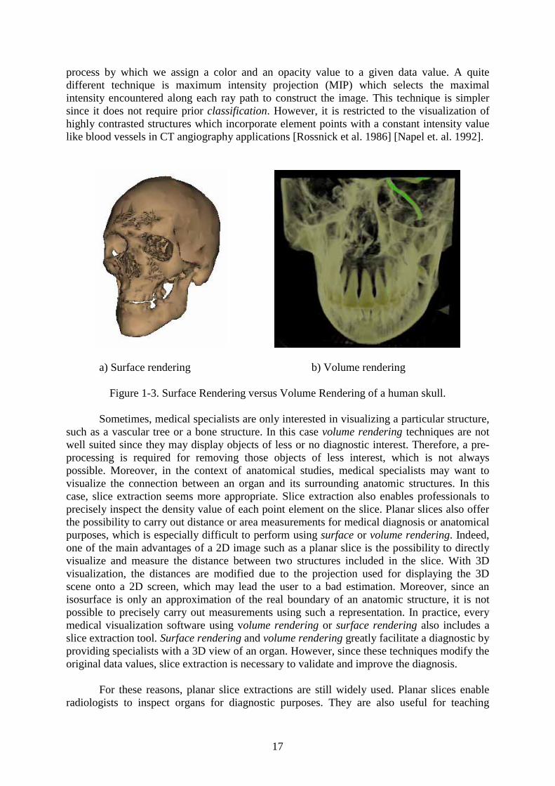
of extraction of a planar slice from a volume image. The two other common ways of displaying 3D medical data are surface rendering and volume rendering[Brodlie and Wood 2001]. Fig. 1-3 presents the visualization of a human skull using surface rendering and volume rendering.
Figure 1-2. Extraction of a planar slice from a volume image.
Surface rendering is an indirect method to obtain an image from a volume dataset. The surfaces of anatomic structures are produced by mapping data values onto a set of geometric primitives in a process known as isosurfacing. These isosurfaces can then be rendered into a displayable image using standard computer graphics techniques and hardware acceleration on most PC graphic cards. The first step for creating isosurfaces is the segmentation of the structure that users want to display, i.e. the selection of all voxels belonging to this structure. Segmentation is a crucial process in surface rendering, since it conditions the quality of the resulting surface. Segmentation may be either manual, i.e. a specialist decides for each slice of the volume image which points are included in the structure or automatic using segmentationalgorithms. Once the segmentation has been performed, the isosurface may be computed using the Marching Cubes algorithm [Wyvill et. al. 1986;Lorensen and Cline 1987]. While this method works well for some data sets, it breaks down when there are small details of a similar scale to the gridsize, and when well-defined surfaces do not exist. These issues, along with the problem of losing the original data, led to the development of another class of algorithms, volume rendering.
Volume rendering is a technique for directly displaying a sampled 3D scalar field without first fitting geometric primitives to the samples. Volume rendering techniques are often based on modelling the data as a translucent gel. The volume dataset may be then rendered to the screen in a variety of ways using ray-casting, splatting[Brodlie and Wood 2001] [Meißner et. al. 2000] or maximum intensity projection (MIP) [Mroz et. al. 2000]. The common approach is to evaluate the dataset along rays at increasing distances from the viewer, and to blend colors to derive pixel intensities. This is called ray-casting and is very similar to ray-tracing. The color at each sample point is acquired by extracting a density value from the dataset, working out which material is at that point, and then looking up the color of that material using a transfer function. Therefore, a fundamental first step is to assign material properties to correspond to the data values. Classification is the
17
process by which we assign a color and an opacity value to a given data value. A quite different technique is maximum intensity projection (MIP) which selects the maximal intensity encountered along each ray path to construct the image. This technique is simpler since it does not require prior classification. However, it is restricted to the visualization of highly contrasted structures which incorporate element points with a constant intensity value like blood vessels in CT angiography applications [Rossnick et al. 1986] [Napel et. al. 1992].
a) Surface rendering b) Volume rendering
Figure 1-3. Surface Rendering versus Volume Rendering of a human skull.
Sometimes, medical specialists are only interested in visualizing a particular structure, such as a vascular tree or a bone structure. In this case volume rendering techniques are not well suited since they may display objects of less or no diagnostic interest. Therefore, a pre-processing is required for removing those objects of less interest, which is not always possible. Moreover, in the context of anatomical studies, medical specialists may want to visualize the connection between an organ and its surrounding anatomic structures. In this case, slice extraction seems more appropriate. Slice extraction also enables professionals to precisely inspect the density value of each point element on the slice. Planar slices also offer the possibility to carry out distance or area measurements for medical diagnosis or anatomical purposes, which is especially difficult to perform using surface or volume rendering. Indeed, one of the main advantages of a 2D image such as a planar slice is the possibility to directly visualize and measure the distance between two structures included in the slice. With 3D visualization, the distances are modified due to the projection used for displaying the 3D scene onto a 2D screen, which may lead the user to a bad estimation. Moreover, since an isosurface is only an approximation of the real boundary of an anatomic structure, it is not possible to precisely carry out measurements using such a representation. In practice, every medical visualization software using volume rendering or surface rendering also includes a slice extraction tool. Surface rendering and volume rendering greatly facilitate a diagnostic by providing specialists with a 3D view of an organ. However, since these techniques modify the original data values, slice extraction is necessary to validate and improve the diagnosis.
For these reasons, planar slice extractions are still widely used. Planar slices enable radiologists to inspect organs for diagnostic purposes. They are also useful for teaching
18
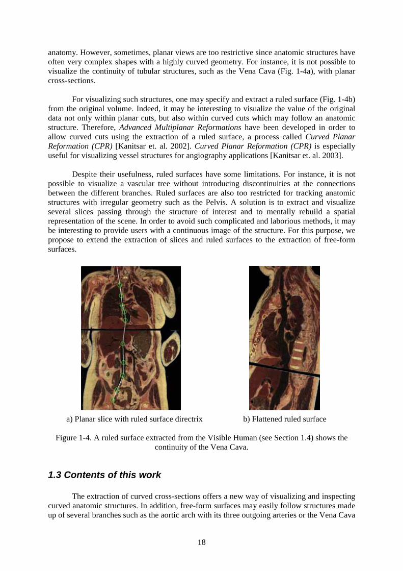
anatomy. However, sometimes, planar views are too restrictive since anatomic structures have often very complex shapes with a highly curved geometry. For instance, it is not possible to visualize the continuity of tubular structures, such as the Vena Cava (Fig. 1-4a), with planar cross-sections.
For visualizing such structures, one may specify and extract a ruled surface (Fig. 1-4b) from the original volume. Indeed, it may be interesting to visualize the value of the original data not only within planar cuts, but also within curved cuts which may follow an anatomic structure. Therefore, Advanced Multiplanar Reformations have been developed in order to allow curved cuts using the extraction of a ruled surface, a process called Curved Planar Reformation (CPR) [Kanitsar et. al. 2002]. Curved Planar Reformation (CPR) is especially useful for visualizing vessel structures for angiography applications [Kanitsar et. al. 2003].
Despite their usefulness, ruled surfaces have some limitations. For instance, it is not possible to visualize a vascular tree without introducing discontinuities at the connections between the different branches. Ruled surfaces are also too restricted for tracking anatomic structures with irregular geometry such as the Pelvis. A solution is to extract and visualize several slices passing through the structure of interest and to mentally rebuild a spatial representation of the scene. In order to avoid such complicated and laborious methods, it may be interesting to provide users with a continuous image of the structure. For this purpose, we propose to extend the extraction of slices and ruled surfaces to the extraction of free-form surfaces.
a) Planar slice with ruled surface directrix b) Flattened ruled surface
Figure 1-4. A ruled surface extracted from the Visible Human (see Section 1.4) shows the continuity of the Vena Cava.
1.3 Contents of this work
The extraction of curved cross-sections offers a new way of visualizing and inspecting curved anatomic structures. In addition, free-form surfaces may easily follow structures made up of several branches such as the aortic arch with its three outgoing arteries or the Vena Cava
19
crossing the atrium cavity (see Fig. 1-4 and Appendix B). Such curved surfaces may provide anatomists with new interesting views that could not be obtained with other techniques. Such surfaces may also track anatomic structures with highly curved geometry. The main objective of this thesis is to propose new methods for the visualization of medical volume images which overcome the limitations of planar slices and existing curved planar reformation techniques, by using interactive extraction and flattening of free-form surfaces.
A first challenge is to define geometric primitives and interactive specification tools for extracting curved surfaces. Indeed, while the extraction of planar slices is straightforward, the specification and extraction of free-form surfaces within 3D volume images may be difficult. For specifying such curved surfaces, it is necessary to define geometric primitives which provide users with a means of controlling the shape and the location of the surface. Moreover, appropriate visualization and interaction tools are required in order to use these geometric primitives for following a structure of interest within a volume image.
Another challenge is to propose an appropriate display of the extracted curved surfaces. Once the surface has been specified and the corresponding texture extracted from the volume image, the most common way to render it onto the computer screen is to use some projection (orthogonal, perspective). However, such projections show some surface parts and may hide other surface parts. The inspection of the whole surface requires changing the viewing point, which may result in missing certain surface parts. Moreover, for anatomical teaching, a global view of the surface is required. In addition, surface projections do not allow users to have a correct estimation of distances or to directly carry out measurements on the textured surface. Surface flattening offers an alternative way of visualizing a surface section [Hacker et. al. 1999] by enabling the visualization of all surface parts within a single planar image. In the general case, surface flattening induces metric and angular distortions. For medical imaging applications, an important objective is the ability to carry out measurements for detecting anatomic abnormalities. Therefore, we propose new flattening algorithms which provide a global view of the surface with a minimum of distortions, and which at the same time enable distance measurements on the flattened surface. Moreover, the flattening algorithms need to be fast and simple in order to be integrated into an application which enables users to interactively extract and flatten any specified surface from a volume image.
These new tools may prove useful for making medical diagnoses and for teaching anatomy. Therefore, we also want to integrate these visualization tools into a Java web application which is freely accessible by medical specialists and others to test the utility and the interest of the free-form surface extraction and flattening. For this purpose, the curved surface extraction and flattening algorithms need to take into account the limitations in memory space, computation times and network bandwidth usage inherent to online applications.
The research work and the results of this thesis are presented in the following chapters. First, Chapter 2 presents fundamental notions from differential geometry necessary to understand our surface specification and flattening methods. In Chapter 3, we introduce an interactive method to specify and extract surfaces following curved anatomic structures. In Chapter 4, we present fundamental notions and existing results on the problem of surface flattening. Then, in Chapter 5, we introduce two different distance preserving flattening methods allowing the visualization of textured curved surfaces within a single planar image. We also show how these methods may be used to carry out distance measurements for anatomical studies. In Chapter 6, we present a method for producing a least distorted flattened
20
surface based on the minimization of the overall geodesic curvature along specific curves on the surface. Finally, the integration of the surface extraction and flattening tools into the Visible Human Server Java applet is presented in Chapter 7.
1.4 The Visible Human dataset
In this work, we propose to develop new visualization tools allowing medical specialists to inspect and visualize anatomic structures using medical volume images. For this purpose, we experiment these new tools on the Visible Human dataset. The Visible Human dataset, produced by the National Library of Medicine’s Visible Human Project [Ackerman 1998], provides an excellent resource for experimenting volume image visualization tools. It consists of transverse CT, MRI, and cryosection imagery of a man. The cryosection dataset provides high-resolution full-color photographs of transverse sections of the human body, representing 13 GB of data. This dataset is a volume of 2048 x 1212 x 1871 voxels, each voxel representing 0.33 x 0.33 x 1 mm. The other datasets (CT, MRI) provide lower resolution grayscale volumes. We used this volume image to test our visualization methods which may be applied to any medical volume image obtained by other standard medical imaging modalities.
21
2 Fundamental notions on curves, surfaces and differential geometry
In this chapter, we recall some definitions about curves, surfaces and differential geometry. Basic properties of parametric surfaces are presented. The definitions of the geodesic and normal curvature of a surface curve are also presented.
2.1 Curves
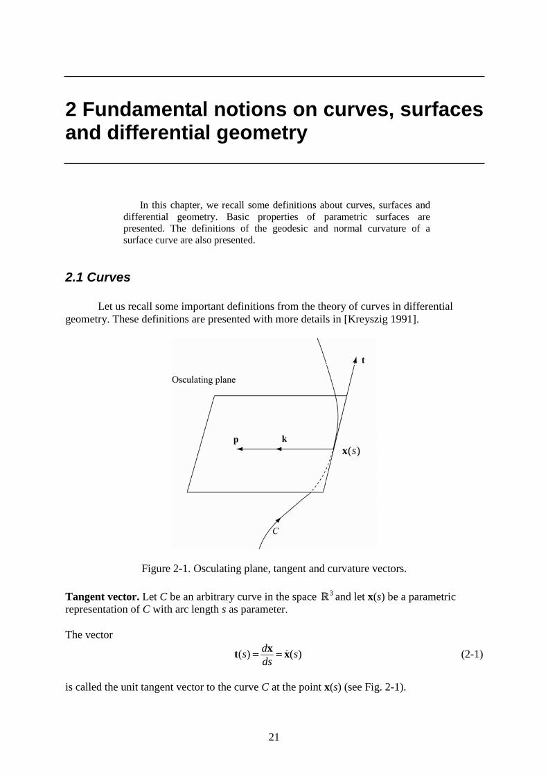
Let us recall some important definitions from the theory of curves in differential geometry. These definitions are presented with more details in [Kreyszig 1991].
Figure 2-1. Osculating plane, tangent and curvature vectors.
Tangent vector. Let C be an arbitrary curve in the space 3 and let x(s) be a parametric representation of C with arc length s as parameter.
The vector
( ) ( )ds sds
= =xt x (2-1)
is called the unit tangent vector to the curve C at the point x(s) (see Fig. 2-1).
( )sx
22
Introducing any other parameter t we have
'' ')
d dtdt ds
= =x xx(x .x
where ' ddt
= xx
Then, '( )'
t = xtx
(2-2)
Osculating plane. Let x(t) be a parametric representation of a curve C. The plane spanned by '( )tx and ''( )tx is called the osculating plane of the curve C at the point x(t).
Principal normal, curvature. Let a curve C be given by a parameterization x(s) with arc length s as parameter. The unit vector
( )( )
( )s
ss
= tpt
(2-3)
which has the direction and the sense of t is called the unit principal normal vector to the curve C at the point x(s) (see Fig. 2-1).
The norm of the vector t ,
( ) ( )k s s= t (2-4)
is called the curvature of the curve C at the point x(s). The reciprocal of the curvature,
1( )( )
sk s
ρ = (2-5)
is called the radius of curvature of the curve C at the point x(s). The vector ( ) ( )s s=k t is called the curvature vector of the curve C (see Fig. 2-1).
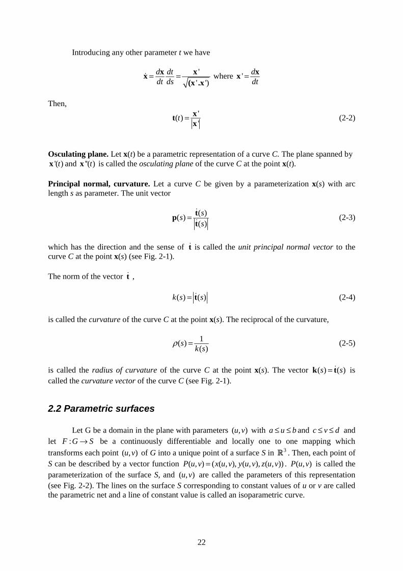
2.2 Parametric surfaces
Let G be a domain in the plane with parameters ( , )u v with a u b≤ ≤ and c v d≤ ≤ and let :F G S→ be a continuously differentiable and locally one to one mapping which
transforms each point ( , )u v of G into a unique point of a surface S in 3 . Then, each point of S can be described by a vector function ( , ) ( ( , ), ( , ), ( , ))P u v x u v y u v z u v= . ( , )P u v is called the parameterization of the surface S, and ( , )u v are called the parameters of this representation (see Fig. 2-2). The lines on the surface S corresponding to constant values of u or v are called the parametric net and a line of constant value is called an isoparametric curve.
23
Figure 2-2. Parameterization of a surface.
A parameterization is said to be regular provided that at every point of S, the normal vector is defined, i.e.
( , ) ( , ) 0u vu v u v× ≠P P (2-6)
In this case, the unit normal vector to S at point ( , )P u v is:
( , ) ( , )( , )
( , ) ( , )u v
u v
u v u vu v
u v u v×=×
P PN
P P (2-7)
and the tangent plane at ( , )P u v is well defined as the plane spanned by ( , )u u vP and ( , )v u vP .
In the next chapters, we use the term parametric surface to refer to a surface described in parametric form ( , ) ( ( , ), ( , ), ( , ))P u v x u v y u v z u v= .
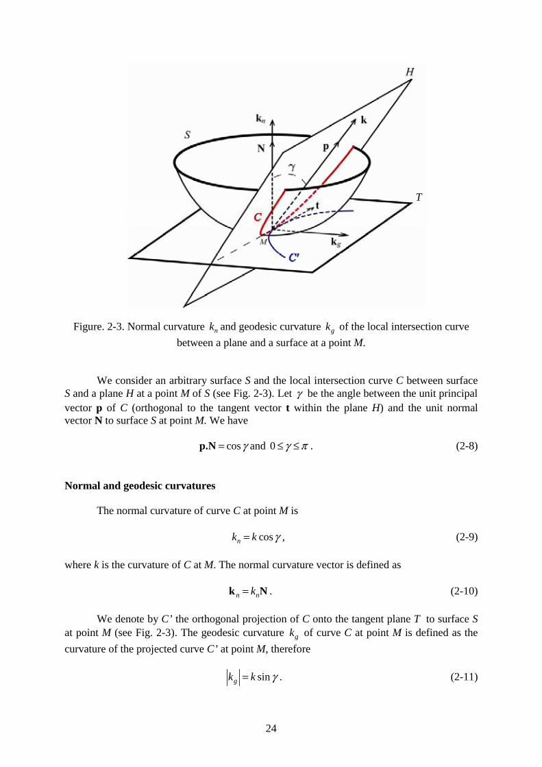
2.3 Geodesic and normal curvature of a surface curve
2.3.1 Definitions
Let us briefly recall the notions of normal curvature, geodesic curvature, principal curvatures, mean curvature and Gaussian curvature [Kreyszig 1991].
24
Figure. 2-3. Normal curvature nk and geodesic curvature gk of the local intersection curve
between a plane and a surface at a point M.
We consider an arbitrary surface S and the local intersection curve C between surface S and a plane H at a point M of S (see Fig. 2-3). Let γ be the angle between the unit principal vector p of C (orthogonal to the tangent vector t within the plane H) and the unit normal vector N to surface S at point M. We have
cosγ=p.N and 0 γ π≤ ≤ . (2-8)
Normal and geodesic curvatures
The normal curvature of curve C at point M is
cosnk k γ= , (2-9)
where k is the curvature of C at M. The normal curvature vector is defined as
n nk=k N . (2-10)
We denote by C’ the orthogonal projection of C onto the tangent plane T to surface Sat point M (see Fig. 2-3). The geodesic curvature gk of curve C at point M is defined as the
curvature of the projected curve C’ at point M, therefore
singk k γ= . (2-11)
T
25
Let t be the tangent direction vector to curve C at point M, i.e. the direction of the intersection between the plane H and the tangent plane to S at M ( 0=p.t ). The value of nk
depends only on the direction of the tangent vector t (Meusnier’s Theorem, [Kreyszig 1991, p. 121]), i.e the normal curvature nk is independent of the γ value:
cosnk k constγ= = (2-12)
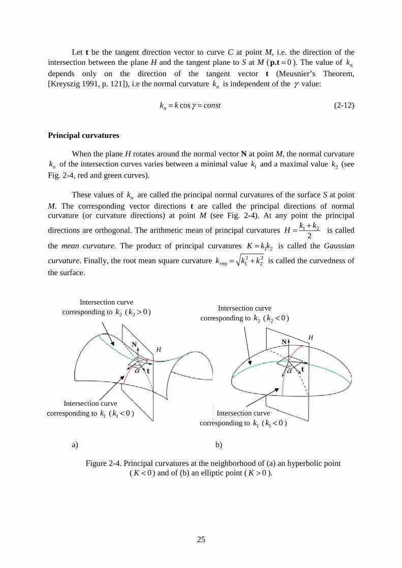
Principal curvatures
When the plane H rotates around the normal vector N at point M, the normal curvature
nk of the intersection curves varies between a minimal value 1k and a maximal value 2k (see
Fig. 2-4, red and green curves).
These values of nk are called the principal normal curvatures of the surface S at point
M. The corresponding vector directions t are called the principal directions of normal curvature (or curvature directions) at point M (see Fig. 2-4). At any point the principal
directions are orthogonal. The arithmetic mean of principal curvatures 1 2
2k k
H+= is called
the mean curvature. The product of principal curvatures 1 2K k k= is called the Gaussian
curvature. Finally, the root mean square curvature 2 21 2rmsk k k= + is called the curvedness of
the surface.
a) b)
Figure 2-4. Principal curvatures at the neighborhood of (a) an hyperbolic point ( 0K < ) and of (b) an elliptic point ( 0K > ).
N N
α αt t
Intersection curve corresponding to 1k ( 1 0k < )
Intersection curve corresponding to 2k ( 2 0k > ) Intersection curve
corresponding to 2k ( 2 0k < )
H
H
Intersection curve corresponding to 1k ( 1 0k < )
26
Let α be the angle between the tangent direction t at a point M and the principal direction at M corresponding to 1k . The following relation holds (Euler’s Theorem,
[Kreyszig 1991, p. 132]):
2 21 2cos sinnk k kα α= + (2-13)
Accordingly, at any point M on a surface S the following relation holds for the normal curvature nk of the intersection curve between surface S and a certain plane H:
1 2nk k k≤ ≤ (2-14)
2.3.2 Calculation of principal curvatures
In this section, we present the calculation of principal curvatures according to [Hoschek and Lasser 1993, pp. 48-49], as well as the calculation of the Mean, Gaussian and root mean square curvatures.
Let ( , )P u v be a parametric representation of the surface S. With uP and vP being the
partial derivatives of P in respect to u and v, we denote
u uE = P .P , u vF = P .P , v vG = P .P
uuL = P .N , uvM = P .N , vvN = P .N
The mean curvature is
H = nk< > = 1 22
1 22 2
k k EN FM GLEG F
+ − +=−
(2-15)
the Gaussian curvature is 2
1 2 2LN MK k kEG F
−= =−
(2-16)
and the principal curvatures are
21
22
k H H K
k H H K
= − −
= + − (2-17)
From which, we can derive
2 2 21 2 4 2rmsk k k H K= + = − (2-18)
27
3 Curved surface extraction for exploring anatomic structures
In this chapter, we present methods allowing the interactive extraction of textured curved surfaces from medical volume images. The challenge resides in offering interaction means facilitating the specification of surfaces following curved anatomic structures within a 3D volume. To meet this challenge, we introduce surface specification tools which rely on interactive slicing and on the placement of marker points inside the volume.
3.1 Previous work on curved surface extraction
In order to provide users with means of inspecting structures having curved geometry, Advanced Multiplanar Reformations have been developed in order to allow curved cuts within a volume image, a process called Curved Planar Reformation (CPR). With Curved Planar Reformation, interesting views of vascular morphology along tortuous paths may be created [He et. al. 2001; Kanitsar et. al. 2003].
Curved Planar Reformation (CPR), i.e. a section through the volume using a ruled surface, is now an established technique in the medical community. Kanitsar et. al. [2002] present a survey of CPR methods for angiography applications. They compare three methods for CPR generation: projected CPR, stretched CPR and straightened CPR. In addition, three extensions to CPR have been proposed to overcome the most relevant clinical limitations: thick CPR, rotating CPR and multi-path CPR. The latter provides a display of a whole vascular tree within one image. While superimposition of bones and arteries is prevented, the intersection of arteries itself is not avoided. In Kanitsar et al. [2003], authors present a new method enabling the visualization of an entire vascular tree using the extraction and flattening of multiple ruled surfaces. These multiple surfaces are flattened onto the same image by avoiding self intersections but discontinuities are unavoidable at the connections between the different surfaces. Further information about the clinical relevance of the CPR visualization technique can be found in [Achenbach et al. 1998; Kanitsar et. al. 2003; Rubin et al. 2001]. A comparison of this technique with conventional volume visualization techniques may be found in [Addis et. al. 2001].
Despite their usefulness, these methods seem restricted to the extraction of ruled surfaces passing through vessel structures. However, it may be interesting to apply this technique to other anatomic structures. For this purpose, Figueiredo and Hersch [2002] present a simple approach for specifying a ruled surface by allowing the user to specify a 2D trajectory on an oblique slice and define the ruling vector perpendicular to this slice. This provides users with interactive means of creating a ruled surface passing through anatomic structures. In the next section, we propose to extend this interactive specification by allowing
28
users to specify a 3D trajectory defining the ruled surface within the volume image. Such an interactive extraction may provide anatomical specialists with a way to create and extract ruled surfaces passing through any anatomic structure.
Unfortunately, as we have seen earlier, ruled surfaces do not allow the visualization of structures with many branches such as an arterial tree without introducing discontinuities. Moreover, ruled surfaces are also too restricted for tracking anatomic structures with irregular geometry such as the Pelvis. For these reasons, we propose to extend Curved Planar Reformation to the extraction of free form surfaces [Saroul et. al. 2003]. In contrast to planar slices and ruled surfaces, free-form surfaces may follow highly curved anatomic structures. These curved surfaces may then be used to visualize branching structures without introducing discontinuities, by extracting a surface passing through the different branches of a tubular structure. We therefore present the method we developed to interactively specify and extract free-form surfaces passing through curved anatomic structures.
First, we present in Section 3.2 and 3.3 geometric primitives that we use for extracting ruled and free-form surfaces from volume images, together with several examples of applications of these surface extractions. Then, we introduce in Section 3.4 interactive tools allowing users to accurately specify surfaces following anatomic structures using these primitives. Finally, in Section 3.5, we explain how free-form surface extractions may be used for exploring anatomy.
3.2 Ruled surface extraction from 3D volume images
3.2.1 Specification and extraction of a ruled surface
We first consider ruled surfaces for tracking curved anatomic structures. We focus on ruled surfaces with a directrix ( )tα and a ruling vector of constant orientation p :
( , ) ( )t tσ ν α ν= + p (3-1)
Such ruled surfaces (also called cylinders) are developable and easy to define, since they only require the definition of the directrix ( )tα and of the ruling vector p . A ruled surface may therefore be easily specified by a 2D natural spline (see Appendix A) located in a planar cross-section, with its ruling vector orthogonal to that cross-section (Fig. 1-4). That is essentially the method proposed in [Figueiredo and Hersch 2002].
However, a ruled surface whose directrix is located within a plane is difficult to use for visualizing non-planar tubular structures such as the aorta. To provide users with a means for specifying ruled surfaces following such a structure, it is necessary to use true 3D trajectories as directrix ( )tα .
As a ruling vector, we choose a vector orthogonal to the main orientations of the curve. Indeed, if the ruling vector is not adequately chosen, two ruling lines 1( , )tσ ν and
2( , )tσ ν may become identical, i.e. 1 2( , ) ( , )t tσ ν σ ν≡ . Structures intersected by these lines
may then be present at two different locations within the resulting flattened surface, making the image interpretation difficult. Compared with [Kanitsar et. al. 2002] where the ruling vector has a fixed orientation within the (Oxy) plane, our method computes the most adequate
29
ruling vector automatically by avoiding as much as possible cases where ruling lines become identical. In order to offer additional freedom and improve the visualization, users are allowed to rotate the ruling vector in the plane orthogonal to the main orientation of the 3D trajectory.
The main orientations of the 3D trajectory are computed using principal component analysis. The trajectory is first represented by a polyline, i.e. a set of discretization points
1 2{ , ,...., }nS = x x x .
We compute the center of gravity G (with coordinates Gx ) of this set, and the
covariance matrix B, taking into account G and all points of S:
1
1( ).( )
1
nT
i G i Gi
Bn =
= − −−
x x x x (3-2)
Since covariance matrix B is definite, positive and symmetric, the normalized eigenvectors of B form a local coordinate system ( , )a b cG x , x ,x with center G and axes
a b cx , x , x . Vector cx is the vector orthogonal to the plane of principal components
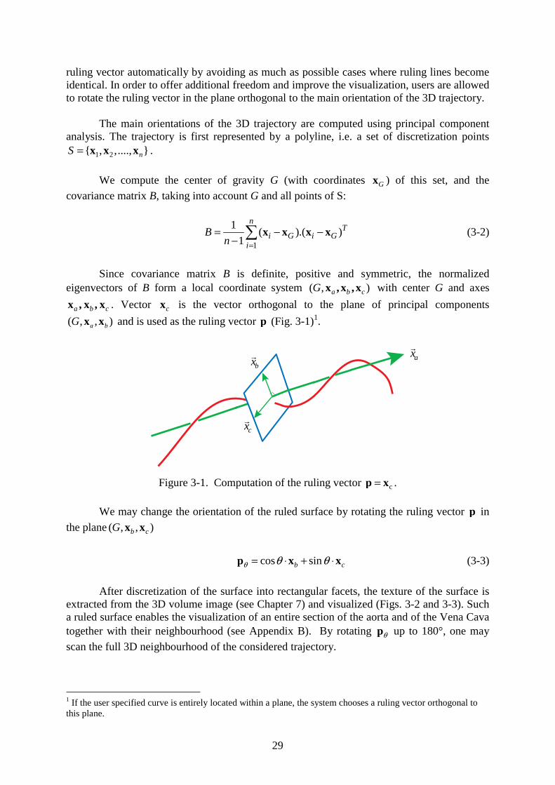
( , , )a bG x x and is used as the ruling vector p (Fig. 3-1)1.
Figure 3-1. Computation of the ruling vector c=p x .
We may change the orientation of the ruled surface by rotating the ruling vector p in
the plane ( , , )b cG x x
cos sinb cθ θ θ= ⋅ + ⋅p x x (3-3)
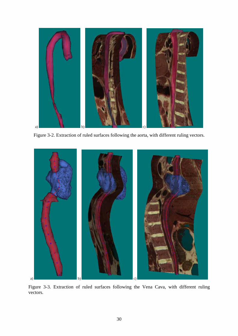
After discretization of the surface into rectangular facets, the texture of the surface is extracted from the 3D volume image (see Chapter 7) and visualized (Figs. 3-2 and 3-3). Such a ruled surface enables the visualization of an entire section of the aorta and of the Vena Cava together with their neighbourhood (see Appendix B). By rotating θp up to 180°, one may
scan the full 3D neighbourhood of the considered trajectory.
1 If the user specified curve is entirely located within a plane, the system chooses a ruling vector orthogonal to this plane.
axbx
cx
30
a) b) c)
Figure 3-2. Extraction of ruled surfaces following the aorta, with different ruling vectors.
a) b) c)
Figure 3-3. Extraction of ruled surfaces following the Vena Cava, with different ruling vectors.
31
3.2.2 Flattening of a ruled surface for visualization
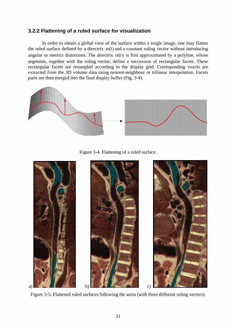
In order to obtain a global view of the surface within a single image, one may flatten the ruled surface defined by a directrix ( )tα and a constant ruling vector without introducing angular or metrics distortions. The directrix ( )tα is first approximated by a polyline, whose segments, together with the ruling vector, define a succession of rectangular facets. These rectangular facets are resampled according to the display grid. Corresponding voxels are extracted from the 3D volume data using nearest-neighbour or trilinear interpolation. Facets parts are then merged into the final display buffer (Fig. 3-4).
Figure 3-4. Flattening of a ruled surface.
a) b) c)
Figure 3-5. Flattened ruled surfaces following the aorta (with three different ruling vectors).
32
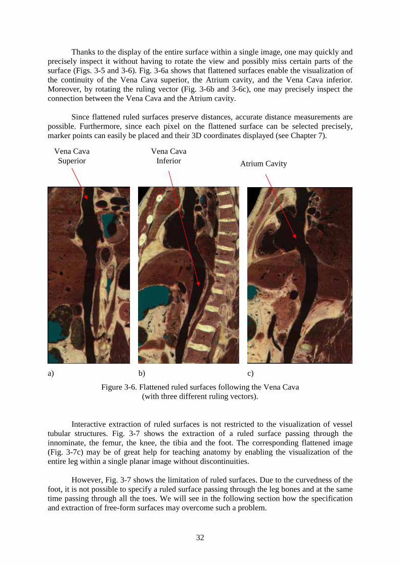
Thanks to the display of the entire surface within a single image, one may quickly and precisely inspect it without having to rotate the view and possibly miss certain parts of the surface (Figs. 3-5 and 3-6). Fig. 3-6a shows that flattened surfaces enable the visualization of the continuity of the Vena Cava superior, the Atrium cavity, and the Vena Cava inferior. Moreover, by rotating the ruling vector (Fig. 3-6b and 3-6c), one may precisely inspect the connection between the Vena Cava and the Atrium cavity.
Since flattened ruled surfaces preserve distances, accurate distance measurements are possible. Furthermore, since each pixel on the flattened surface can be selected precisely, marker points can easily be placed and their 3D coordinates displayed (see Chapter 7).
a) b) c)
Figure 3-6. Flattened ruled surfaces following the Vena Cava (with three different ruling vectors).
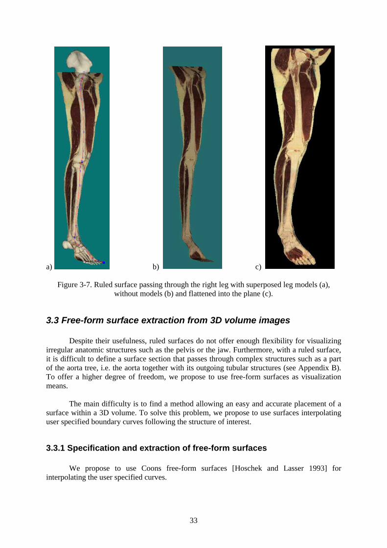
Interactive extraction of ruled surfaces is not restricted to the visualization of vessel tubular structures. Fig. 3-7 shows the extraction of a ruled surface passing through the innominate, the femur, the knee, the tibia and the foot. The corresponding flattened image (Fig. 3-7c) may be of great help for teaching anatomy by enabling the visualization of the entire leg within a single planar image without discontinuities.
However, Fig. 3-7 shows the limitation of ruled surfaces. Due to the curvedness of the foot, it is not possible to specify a ruled surface passing through the leg bones and at the same time passing through all the toes. We will see in the following section how the specification and extraction of free-form surfaces may overcome such a problem.
Atrium Cavity
Vena Cava Superior
Vena Cava Inferior
33
a) b) c)
Figure 3-7. Ruled surface passing through the right leg with superposed leg models (a), without models (b) and flattened into the plane (c).
3.3 Free-form surface extraction from 3D volume images
Despite their usefulness, ruled surfaces do not offer enough flexibility for visualizing irregular anatomic structures such as the pelvis or the jaw. Furthermore, with a ruled surface, it is difficult to define a surface section that passes through complex structures such as a part of the aorta tree, i.e. the aorta together with its outgoing tubular structures (see Appendix B). To offer a higher degree of freedom, we propose to use free-form surfaces as visualization means.
The main difficulty is to find a method allowing an easy and accurate placement of a surface within a 3D volume. To solve this problem, we propose to use surfaces interpolating user specified boundary curves following the structure of interest.
3.3.1 Specification and extraction of free-form surfaces
We propose to use Coons free-form surfaces [Hoschek and Lasser 1993] for interpolating the user specified curves.
34
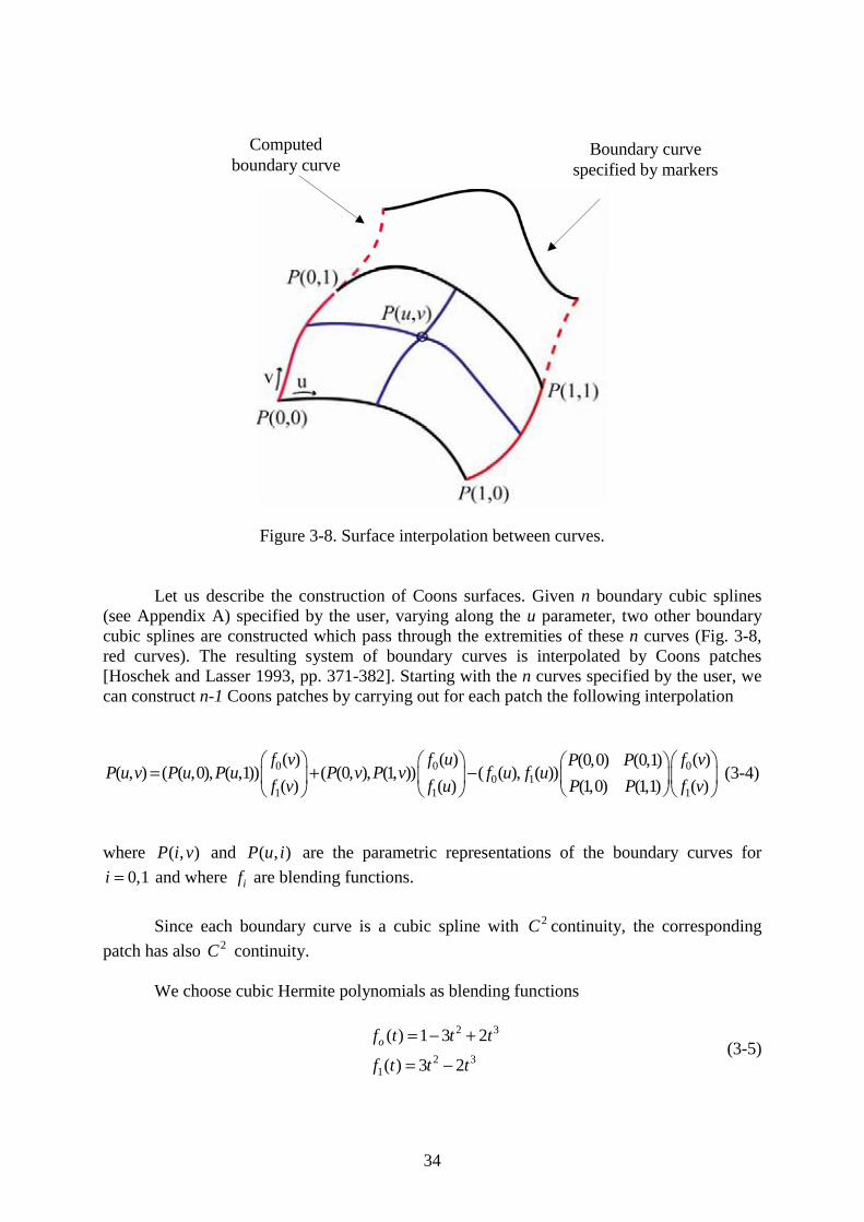
Figure 3-8. Surface interpolation between curves.
Let us describe the construction of Coons surfaces. Given n boundary cubic splines (see Appendix A) specified by the user, varying along the u parameter, two other boundary cubic splines are constructed which pass through the extremities of these n curves (Fig. 3-8, red curves). The resulting system of boundary curves is interpolated by Coons patches [Hoschek and Lasser 1993, pp. 371-382]. Starting with the n curves specified by the user, we can construct n-1 Coons patches by carrying out for each patch the following interpolation
0 0 00 1
1 1 1
( ) ( ) ( )(0,0) (0,1)( , ) ( ( ,0), ( ,1)) ( (0, ), (1, )) ( ( ), ( ))
(1,0) (1,1)( ) ( ) ( )
f v f u f vP PP u v P u P u P v P v f u f u
P Pf v f u f v= + − (3-4)
where ( , )P i v and ( , )P u i are the parametric representations of the boundary curves for
0,1i = and where if are blending functions.
Since each boundary curve is a cubic spline with 2C continuity, the corresponding
patch has also 2C continuity.
We choose cubic Hermite polynomials as blending functions
2 3
2 31
( ) 1 3 2
( ) 3 2
of t t t
f t t t
= − +
= − (3-5)
Boundary curve specified by markers
Computedboundary curve
35
which satisfy the continuity conditions
1,( )
0,i ik
i kf k
i kδ
== =
≠ and ( ) 0,if k′ = for , 0,1.i k = (3-6)
Thus, derivatives of the patch along boundaries are given by
0 1
0 1
( , ) ( ,0). ( ) ( ,1). ( )
( , ) (0, ). ( ) (1, ). ( )u u u
v v v
P i v P i f v P i f v
P u i P i f u P i f u
= += +
for 0,1.i = (3-7)
Using these functions, the tangent vectors to the curve ( , )cP u v at the point ( ,1)cP u
(with cu constant) depend only on the tangent vectors (0,1)vP and (1,1)vP at points (0,1)P
and (1,1)P . It follows from (3-7) that if the two computed boundary curves have 1C
continuity at these points, the two neighbouring patches A and B join together with 1Ccontinuity along the curve ( ,1) ( ,0)A BP u P u= (Fig. 3-8). In contrast to bi-cubic patches [Hoschek and Lasser 1993, pp. 382-385], the presented bilinear interpolation with cubic Hermite polynomials does not require to specify the derivatives ( ,0),vP u ( ,1),vP u (0, )uP v and
(1, )uP v along boundary curves.
a) Boundary curves specification b) Resulting Curved Surface
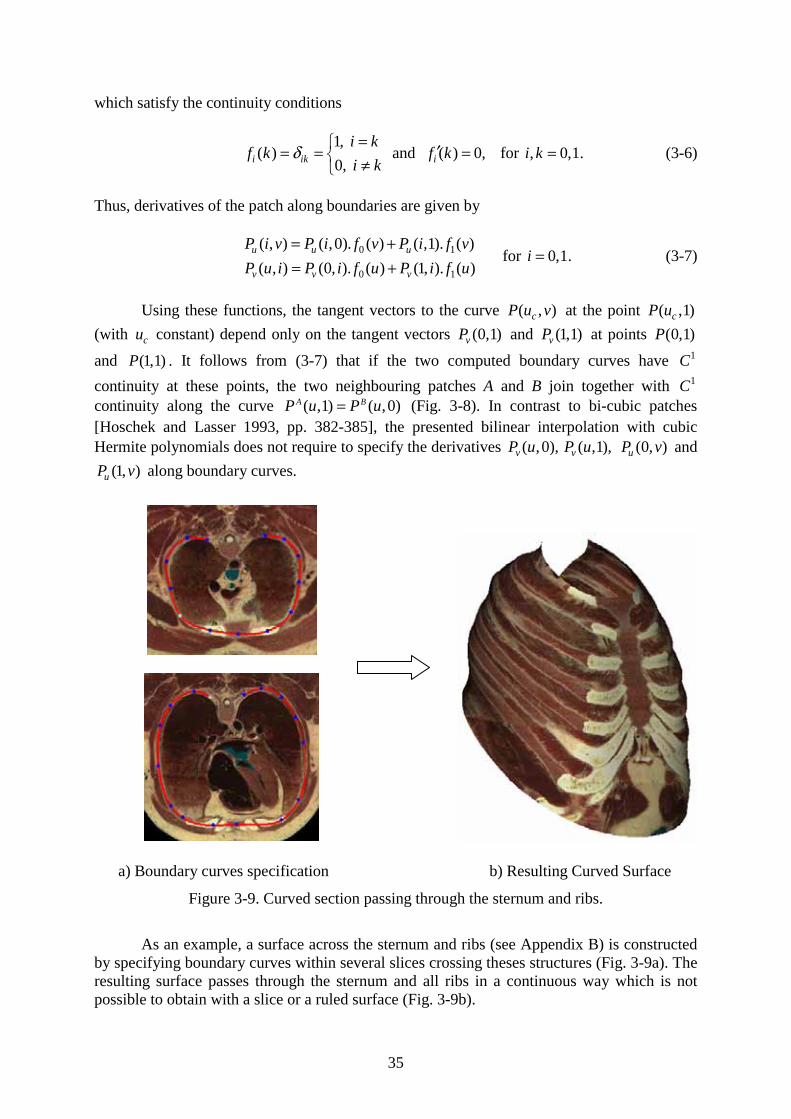
Figure 3-9. Curved section passing through the sternum and ribs.
As an example, a surface across the sternum and ribs (see Appendix B) is constructed by specifying boundary curves within several slices crossing theses structures (Fig. 3-9a). The resulting surface passes through the sternum and all ribs in a continuous way which is not possible to obtain with a slice or a ruled surface (Fig. 3-9b).
36
a) b) c)
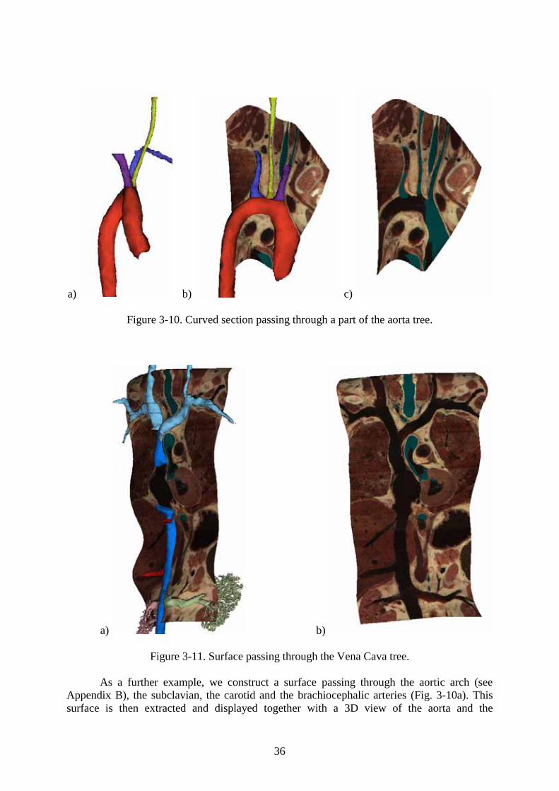
Figure 3-10. Curved section passing through a part of the aorta tree.
a) b)
Figure 3-11. Surface passing through the Vena Cava tree.
As a further example, we construct a surface passing through the aortic arch (see Appendix B), the subclavian, the carotid and the brachiocephalic arteries (Fig. 3-10a). This surface is then extracted and displayed together with a 3D view of the aorta and the
37
corresponding arteries (Fig. 3-10b) or alone (Fig. 3-10c). This illustrates the connections between the aortic arch and the outgoing arteries.
Finally, we construct a surface passing through the Vena Cava tree (Fig. 3-11a, see Appendix B). Unlike a ruled surface which only reveals the continuity of the Vena Cava Superior, the Atrium cavity, and the Vena Cava Superior, this surface enables in addition the visualization of the connections between the Vena Cava and several non coplanar outgoing veins (Fig. 3-11b).
3.3.3 Visualizing free-form textured surfaces using a flattened view
In the previous figures, free-form surfaces are displayed using orthogonal projection on the display screen. In order to facilitate the inspection of the anatomic structures included in such free-form surfaces, we would like to flatten them into the plane. However, Coons surfaces are not developable, i.e. it is not possible to unfold them without distortions. We therefore present in Chapter 5 two different distance flattening methods which try to minimize distortions near a focus point specified by the user.
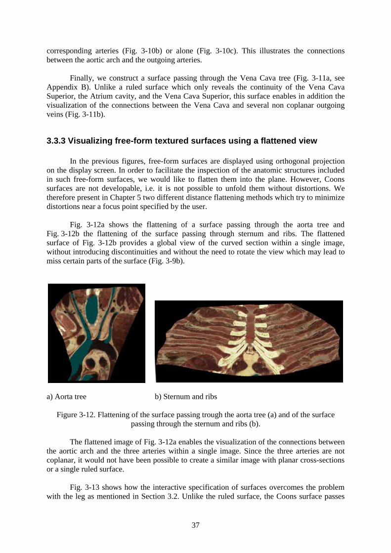
Fig. 3-12a shows the flattening of a surface passing through the aorta tree and Fig. 3-12b the flattening of the surface passing through sternum and ribs. The flattened surface of Fig. 3-12b provides a global view of the curved section within a single image, without introducing discontinuities and without the need to rotate the view which may lead to miss certain parts of the surface (Fig. 3-9b).
a) Aorta tree b) Sternum and ribs
Figure 3-12. Flattening of the surface passing trough the aorta tree (a) and of the surface passing through the sternum and ribs (b).
The flattened image of Fig. 3-12a enables the visualization of the connections between the aortic arch and the three arteries within a single image. Since the three arteries are not coplanar, it would not have been possible to create a similar image with planar cross-sections or a single ruled surface.
Fig. 3-13 shows how the interactive specification of surfaces overcomes the problem with the leg as mentioned in Section 3.2. Unlike the ruled surface, the Coons surface passes
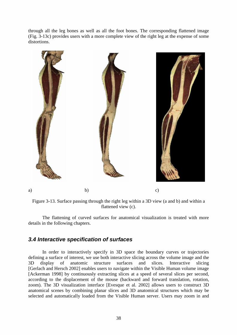
38
through all the leg bones as well as all the foot bones. The corresponding flattened image (Fig. 3-13c) provides users with a more complete view of the right leg at the expense of some distortions.
a) b) c)
Figure 3-13. Surface passing through the right leg within a 3D view (a and b) and within a flattened view (c).
The flattening of curved surfaces for anatomical visualization is treated with more details in the following chapters.
3.4 Interactive specification of surfaces
In order to interactively specify in 3D space the boundary curves or trajectories defining a surface of interest, we use both interactive slicing across the volume image and the 3D display of anatomic structure surfaces and slices. Interactive slicing [Gerlach and Hersch 2002] enables users to navigate within the Visible Human volume image [Ackerman 1998] by continuously extracting slices at a speed of several slices per second, according to the displacement of the mouse (backward and forward translation, rotation, zoom). The 3D visualization interface [Evesque et al. 2002] allows users to construct 3D anatomical scenes by combining planar slices and 3D anatomical structures which may be selected and automatically loaded from the Visible Human server. Users may zoom in and
39
out, rotate and translate the scene as well as displace and rotate the planar slices located within the scene.
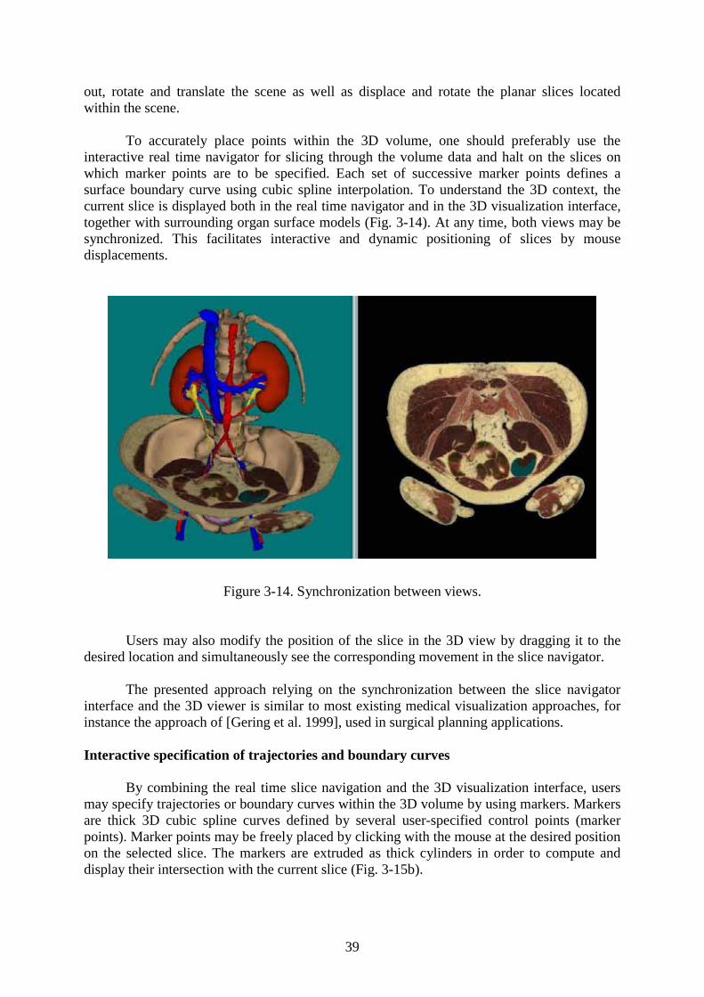
To accurately place points within the 3D volume, one should preferably use the interactive real time navigator for slicing through the volume data and halt on the slices on which marker points are to be specified. Each set of successive marker points defines a surface boundary curve using cubic spline interpolation. To understand the 3D context, the current slice is displayed both in the real time navigator and in the 3D visualization interface, together with surrounding organ surface models (Fig. 3-14). At any time, both views may be synchronized. This facilitates interactive and dynamic positioning of slices by mouse displacements.
Figure 3-14. Synchronization between views.
Users may also modify the position of the slice in the 3D view by dragging it to the desired location and simultaneously see the corresponding movement in the slice navigator.
The presented approach relying on the synchronization between the slice navigator interface and the 3D viewer is similar to most existing medical visualization approaches, for instance the approach of [Gering et al. 1999], used in surgical planning applications.
Interactive specification of trajectories and boundary curves
By combining the real time slice navigation and the 3D visualization interface, users may specify trajectories or boundary curves within the 3D volume by using markers. Markers are thick 3D cubic spline curves defined by several user-specified control points (marker points). Marker points may be freely placed by clicking with the mouse at the desired position on the selected slice. The markers are extruded as thick cylinders in order to compute and display their intersection with the current slice (Fig. 3-15b).
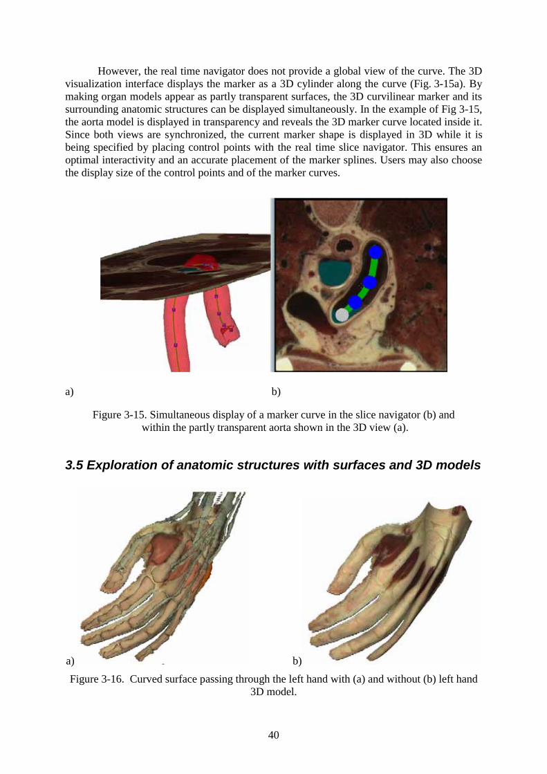
40
However, the real time navigator does not provide a global view of the curve. The 3D visualization interface displays the marker as a 3D cylinder along the curve (Fig. 3-15a). By making organ models appear as partly transparent surfaces, the 3D curvilinear marker and its surrounding anatomic structures can be displayed simultaneously. In the example of Fig 3-15, the aorta model is displayed in transparency and reveals the 3D marker curve located inside it. Since both views are synchronized, the current marker shape is displayed in 3D while it is being specified by placing control points with the real time slice navigator. This ensures an optimal interactivity and an accurate placement of the marker splines. Users may also choose the display size of the control points and of the marker curves.
a) b)
Figure 3-15. Simultaneous display of a marker curve in the slice navigator (b) and within the partly transparent aorta shown in the 3D view (a).
3.5 Exploration of anatomic structures with surfaces and 3D models
a) b)
Figure 3-16. Curved surface passing through the left hand with (a) and without (b) left hand 3D model.
41
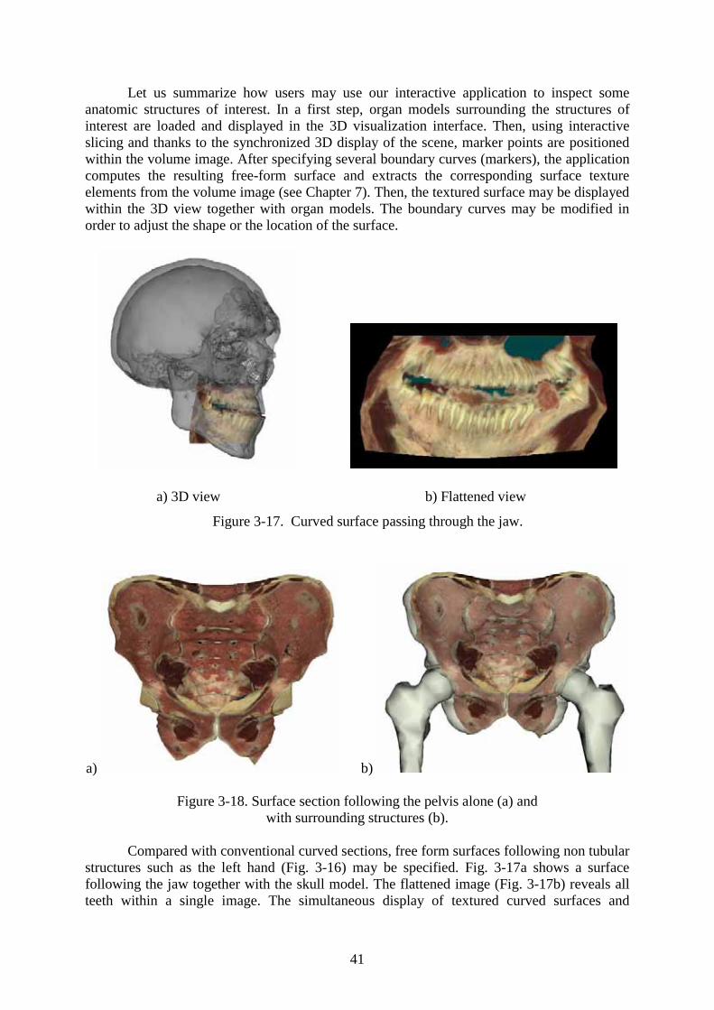
Let us summarize how users may use our interactive application to inspect some anatomic structures of interest. In a first step, organ models surrounding the structures of interest are loaded and displayed in the 3D visualization interface. Then, using interactive slicing and thanks to the synchronized 3D display of the scene, marker points are positioned within the volume image. After specifying several boundary curves (markers), the application computes the resulting free-form surface and extracts the corresponding surface texture elements from the volume image (see Chapter 7). Then, the textured surface may be displayed within the 3D view together with organ models. The boundary curves may be modified in order to adjust the shape or the location of the surface.
a) 3D view b) Flattened view
Figure 3-17. Curved surface passing through the jaw.
a) b)
Figure 3-18. Surface section following the pelvis alone (a) and with surrounding structures (b).
Compared with conventional curved sections, free form surfaces following non tubular structures such as the left hand (Fig. 3-16) may be specified. Fig. 3-17a shows a surface following the jaw together with the skull model. The flattened image (Fig. 3-17b) reveals all teeth within a single image. The simultaneous display of textured curved surfaces and
42
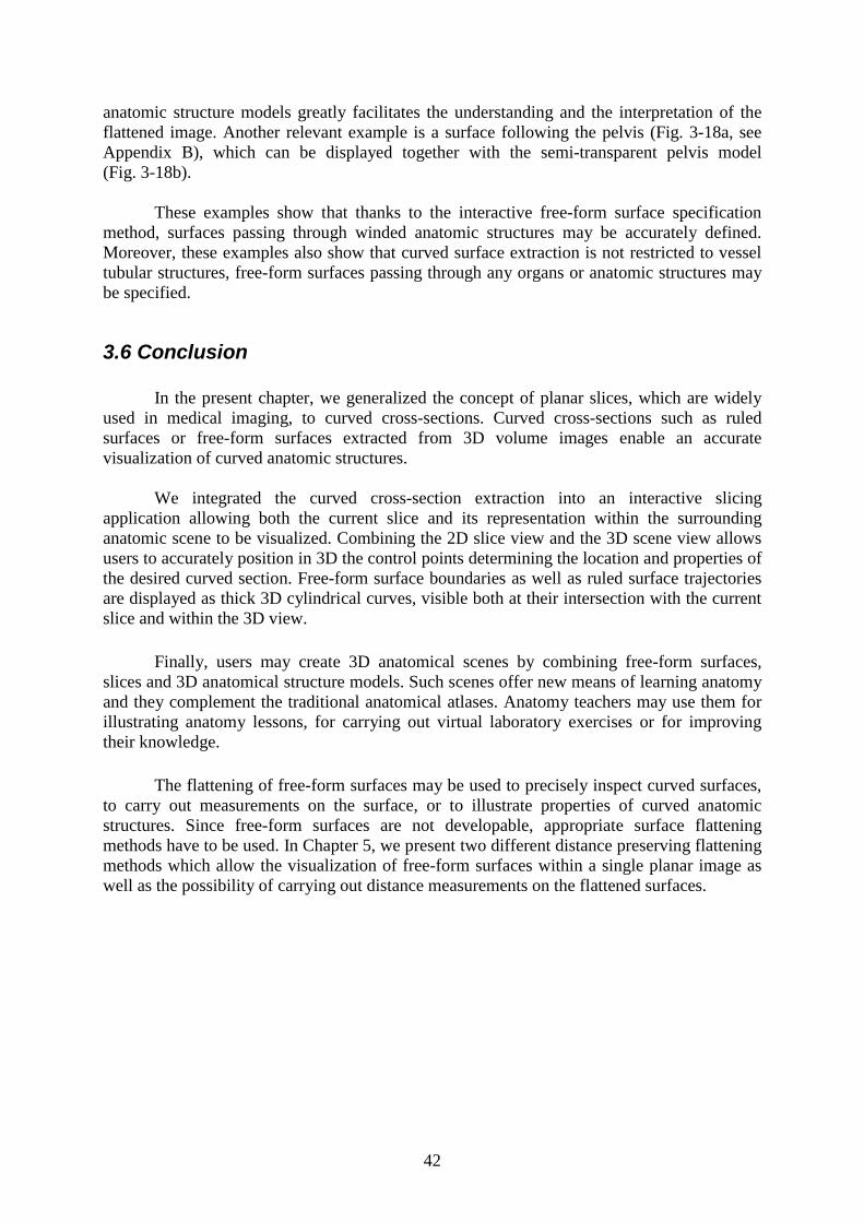
anatomic structure models greatly facilitates the understanding and the interpretation of the flattened image. Another relevant example is a surface following the pelvis (Fig. 3-18a, see Appendix B), which can be displayed together with the semi-transparent pelvis model (Fig. 3-18b).
These examples show that thanks to the interactive free-form surface specification method, surfaces passing through winded anatomic structures may be accurately defined. Moreover, these examples also show that curved surface extraction is not restricted to vessel tubular structures, free-form surfaces passing through any organs or anatomic structures may be specified.
3.6 Conclusion
In the present chapter, we generalized the concept of planar slices, which are widely used in medical imaging, to curved cross-sections. Curved cross-sections such as ruled surfaces or free-form surfaces extracted from 3D volume images enable an accurate visualization of curved anatomic structures.
We integrated the curved cross-section extraction into an interactive slicing application allowing both the current slice and its representation within the surrounding anatomic scene to be visualized. Combining the 2D slice view and the 3D scene view allows users to accurately position in 3D the control points determining the location and properties of the desired curved section. Free-form surface boundaries as well as ruled surface trajectories are displayed as thick 3D cylindrical curves, visible both at their intersection with the current slice and within the 3D view.
Finally, users may create 3D anatomical scenes by combining free-form surfaces, slices and 3D anatomical structure models. Such scenes offer new means of learning anatomy and they complement the traditional anatomical atlases. Anatomy teachers may use them for illustrating anatomy lessons, for carrying out virtual laboratory exercises or for improving their knowledge.
The flattening of free-form surfaces may be used to precisely inspect curved surfaces, to carry out measurements on the surface, or to illustrate properties of curved anatomic structures. Since free-form surfaces are not developable, appropriate surface flattening methods have to be used. In Chapter 5, we present two different distance preserving flattening methods which allow the visualization of free-form surfaces within a single planar image as well as the possibility of carrying out distance measurements on the flattened surfaces.
43
4 Introduction to surface flattening
In this chapter we recall the concept of surface flattening and present the specific requirements in the context of anatomical curved surface visualization. We review previous research works on surface parameterization, and explain their limitations for our application. We finally describe in detail an existing flattening algorithm which is used in the next chapters.
4.1 Introduction
The surface flattening problem is linked to the more general problem of finding a parameterization of a surface. Indeed, as surface flattening, a parameterization of a surface consists of finding a one-to-one mapping from the surface to a planar domain (see Chapter 2). Parameterizations have many applications in various fields of science and engineering. The main application of parameterization in computer graphics is texture mapping which is used to map a planar image onto polygonal models.
Parameterizations, mapping, or flattening of 3D surfaces almost always induce distortions in either angles, lengths or areas. To evaluate the quality of a mapping in an application, it is necessary to first decide which kind of distortions have to be minimized or what properties need to be preserved. A good mapping for a given application is the one which meets these requirements.
For our anatomical surface visualization application, the first requirement is to produce a flattened surface without cuts in order to provide users with a continuous view of the whole surface. In order to precisely inspect a region of interest with high precision, the distortions have to be minimized near a user specified focus point on the surface. Then, users may move this focus point and successively inspect each surface part. We also want to provide users with the means of carrying out measurements on the surface. For this purpose, distances should be preserved along user specified orientations. Finally, the surface flattening algorithm needs to be fast and simple in order to be integrated into a software allowing users to interactively visualize flattened curved surfaces.
We first recall the general surface parameterization problem (Section 4.2) in complement of the definitions from differential geometry presented in Chapter 2. Then, we present previous research works on this topic and show that a new flattening algorithm needs to be proposed (Section 4.3). For this purpose, we present in detail an existing flattening algorithm incorporating interesting techniques which is used in our algorithm (Section 4.4).
44
4.2 Surface parameterization concept
Let us briefly recall the general concept of surface parameterization, i.e. one-to-one mapping from a surface to a planar domain. The theory of mapping is a vast mathematical problem. In this section, we only recall some important definitions necessary to understand the rest of this work. Please refer to [Cohn 1980], [Kreiszig et. al. 1991] and [Floater and Hormann 2004] for more detailed explanations on the mathematical concept.
4.2.1 Mapping definition
Let S and S* be two set of points in three-dimensional Euclidean space. If a rule T is stated which associates a point P’ of S* to every point P of S, we say that a transformation of the set S into S* is given. P’ is called the image point of P, and P is called an inverse image point of P’. The set of the image points of all points of S is called the image of S. If every point of S* is an image point of at least one point of S the transformation T is called a mapping of S onto S*.
A mapping T of S onto S* is called one-to-one if the image points of any pair of different points of S are different points of S*. Then there exists the inverse mapping of T,denoted by 1T − . 1T − map S* onto S such that every point P’ of S* is mapped onto a point Pof S which is the inverse image of to P’ under the mapping T.
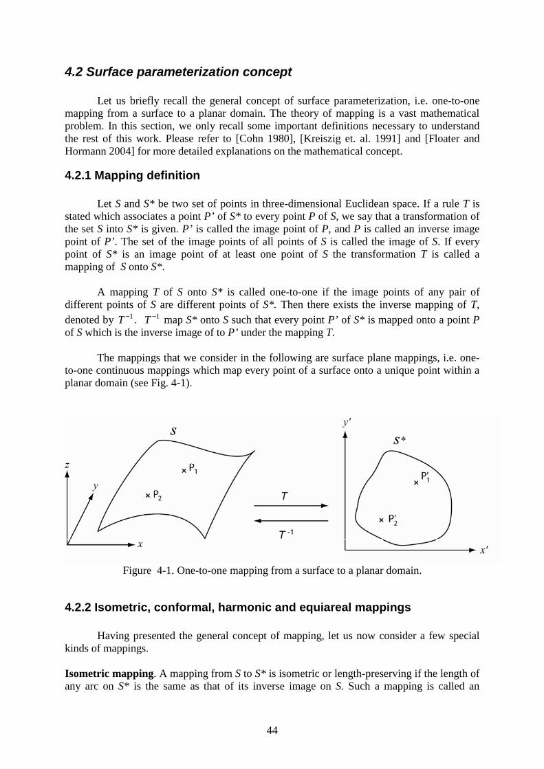
The mappings that we consider in the following are surface plane mappings, i.e. one-to-one continuous mappings which map every point of a surface onto a unique point within a planar domain (see Fig. 4-1).
Figure 4-1. One-to-one mapping from a surface to a planar domain.
4.2.2 Isometric, conformal, harmonic and equiareal mappings
Having presented the general concept of mapping, let us now consider a few special kinds of mappings.
Isometric mapping. A mapping from S to S* is isometric or length-preserving if the length of any arc on S* is the same as that of its inverse image on S. Such a mapping is called an
45
isometry. For example, the mapping of a cylinder into the plane that transforms cylindrical coordinates into cartesian coordinates is isometric.
Conformal mapping. A mapping from S to S* is conformal or angle-preserving if the angle of intersection of every pair of intersecting arcs on S* is the same as that of the corresponding inverse images on S at the corresponding point. For instance, the stereographic and Mercator projections are conformal maps from the sphere to the plane (see Fig. 4-5).
Conformal projections of general surfaces are of special interest due to their close connection to the Riemann Mapping Theorem [Cohn 1980]. This theorem states that any simply-connected region of the complex plane can be mapped conformally into any other simply-connected region, such as the unit disk. It therefore implies that any disk-like surface can be mapped conformally into any simply-connected region of the plane. However, there is no method for computing such a mapping in the general case.
Harmonic mapping. A mapping from S to S* which satisfies the two Laplace equations from complex function theory [Cohn 1980] is harmonic. Any conformal mapping is harmonic but the inverse statement is false. The main advantage of harmonic maps compared with conformal maps is that they can be computed, at least approximately [Floater and Hormann 2004]. Moreover such mappings minimize deformation in the sense that they minimize the Dirichlet Energy [Cohn 1980]. Please refer to [Cohn 1980] and [Floater and Hormann 2004] for more information about conformal and harmonic mappings. Equiareal mapping. A mapping from S to S* is equiareal if every part of S is mapped onto a part of S* with the same area. For example, the Lambert projection is an equiareal mapping from the sphere to the plane (see Fig. 4-5).
Every isometric mapping is conformal and equiareal, and every conformal and equiareal mapping is isometric, i.e.
isometric ⇔ conformal + equiareal.
4.2.3 Definitions of surface parameterization, surface flattening and texture mapping.
In differential geometry, the surface parameterization problem consists in associating each point ( , , )x y z of a surface to a unique point ( , )u v in the parameter space. A parameterization ( , ) ( ( , ), ( , ), ( , ))P u v x u v y u v z u v= of a surface as presented in Section 2.2 can then be viewed as a one-to-one mapping from a rectangular planar domain to the surface.
In computer graphics, surface parameterization refers to the more general problem of finding a one to one mapping between a planar domain and the surface.
The surface flattening problem consists in unfolding a surface into the plane. If the surface is unfolded without self-intersections, each point ( , , )x y z of the original surface may be associated with a unique point ( , )x y′ ′ of the flattened surface. A surface parameterization
46
is obtained since a rule T which maps every point ( , , )x y z of the surface into a unique point ( , )x y′ ′ of a planar domain may be defined. Surface flattening is therefore equivalent to determining a surface parameterization.
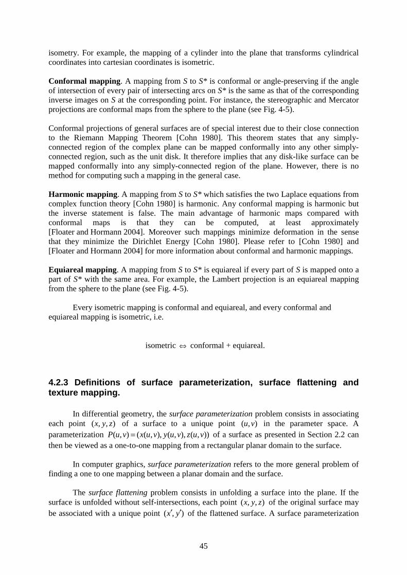
Surface flattening may be used for visualizing within the plane a texture image located on a surface (see Fig. 4-2). The surface S is first sampled into a set of elementary regions { }iS . Given a surface region iS having a color iC and the corresponding image
region iS′ under the transformation T, the color iC may be used as the color of the image
region iS′ within the flattened surface *S (see Fig. 4-2). Using this process for all elementary
surface regions of S leads to a flattened textured surface.
a) Original surface b) Flattened surface
Figure 4-2. Surface flattening.
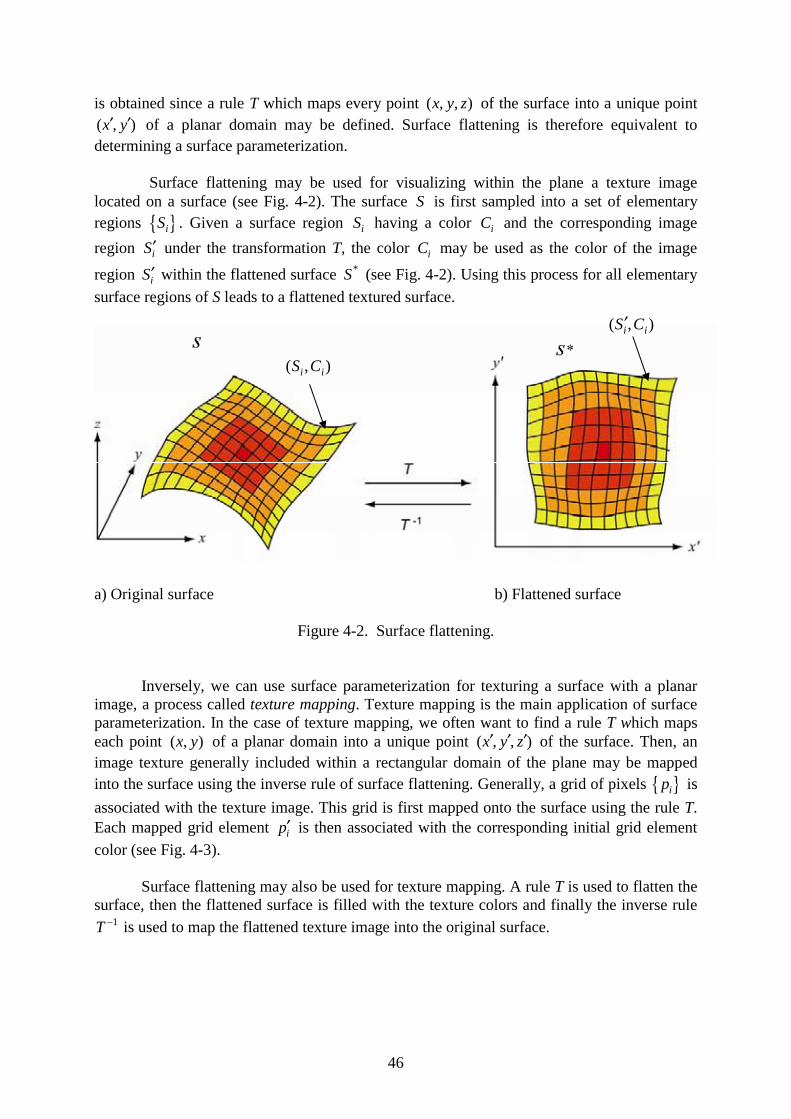
Inversely, we can use surface parameterization for texturing a surface with a planar image, a process called texture mapping. Texture mapping is the main application of surface parameterization. In the case of texture mapping, we often want to find a rule T which maps each point ( , )x y of a planar domain into a unique point ( , , )x y z′ ′ ′ of the surface. Then, an image texture generally included within a rectangular domain of the plane may be mapped into the surface using the inverse rule of surface flattening. Generally, a grid of pixels { }ip is
associated with the texture image. This grid is first mapped onto the surface using the rule T.Each mapped grid element ip′ is then associated with the corresponding initial grid element
color (see Fig. 4-3).
Surface flattening may also be used for texture mapping. A rule T is used to flatten the surface, then the flattened surface is filled with the texture colors and finally the inverse rule
1T − is used to map the flattened texture image into the original surface.
( , )i iS C
( , )i iS C′
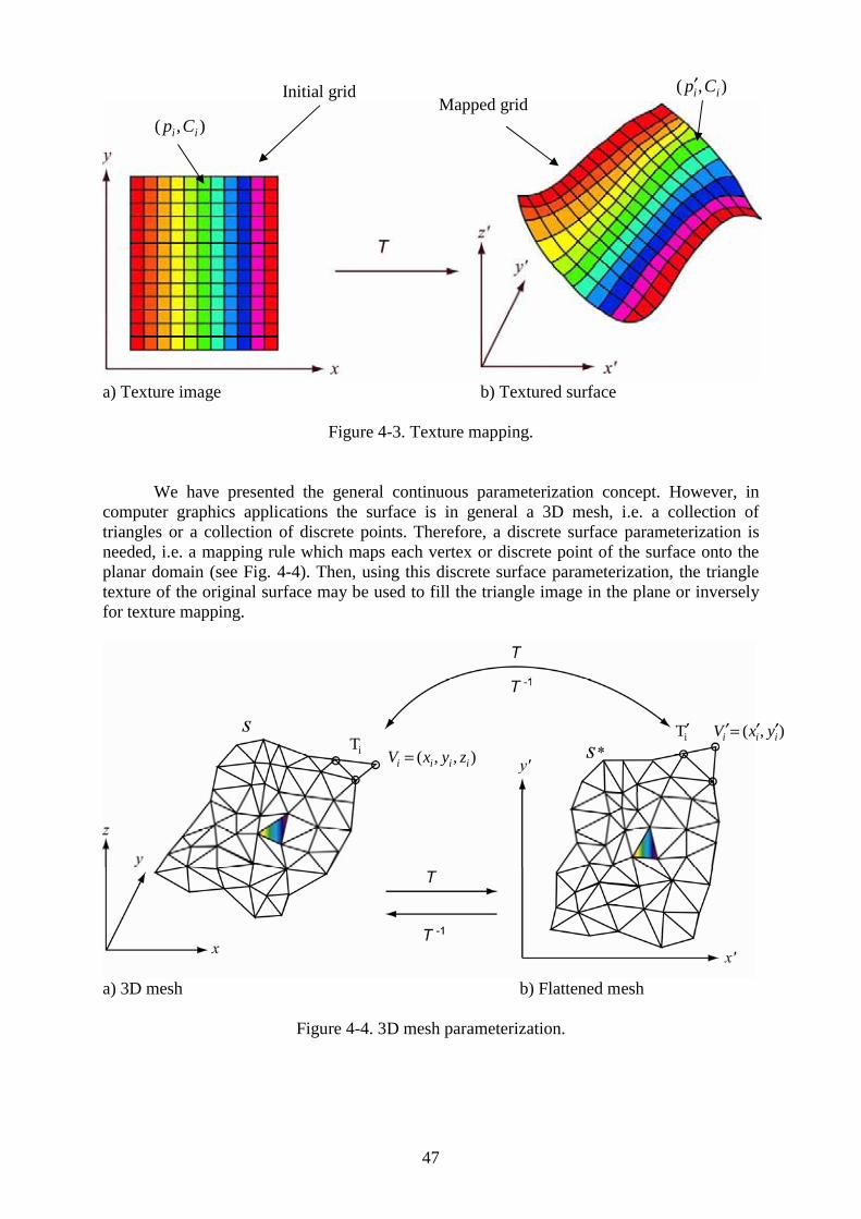
47
a) Texture image b) Textured surface
Figure 4-3. Texture mapping.
We have presented the general continuous parameterization concept. However, in computer graphics applications the surface is in general a 3D mesh, i.e. a collection of triangles or a collection of discrete points. Therefore, a discrete surface parameterization is needed, i.e. a mapping rule which maps each vertex or discrete point of the surface onto the planar domain (see Fig. 4-4). Then, using this discrete surface parameterization, the triangle texture of the original surface may be used to fill the triangle image in the plane or inversely for texture mapping.
a) 3D mesh b) Flattened mesh
Figure 4-4. 3D mesh parameterization.
( , , )i i i iV x y z=( , )i i iV x y′ ′ ′=
iT iT′
( , )i ip C
( , )i ip C′Initial grid Mapped grid
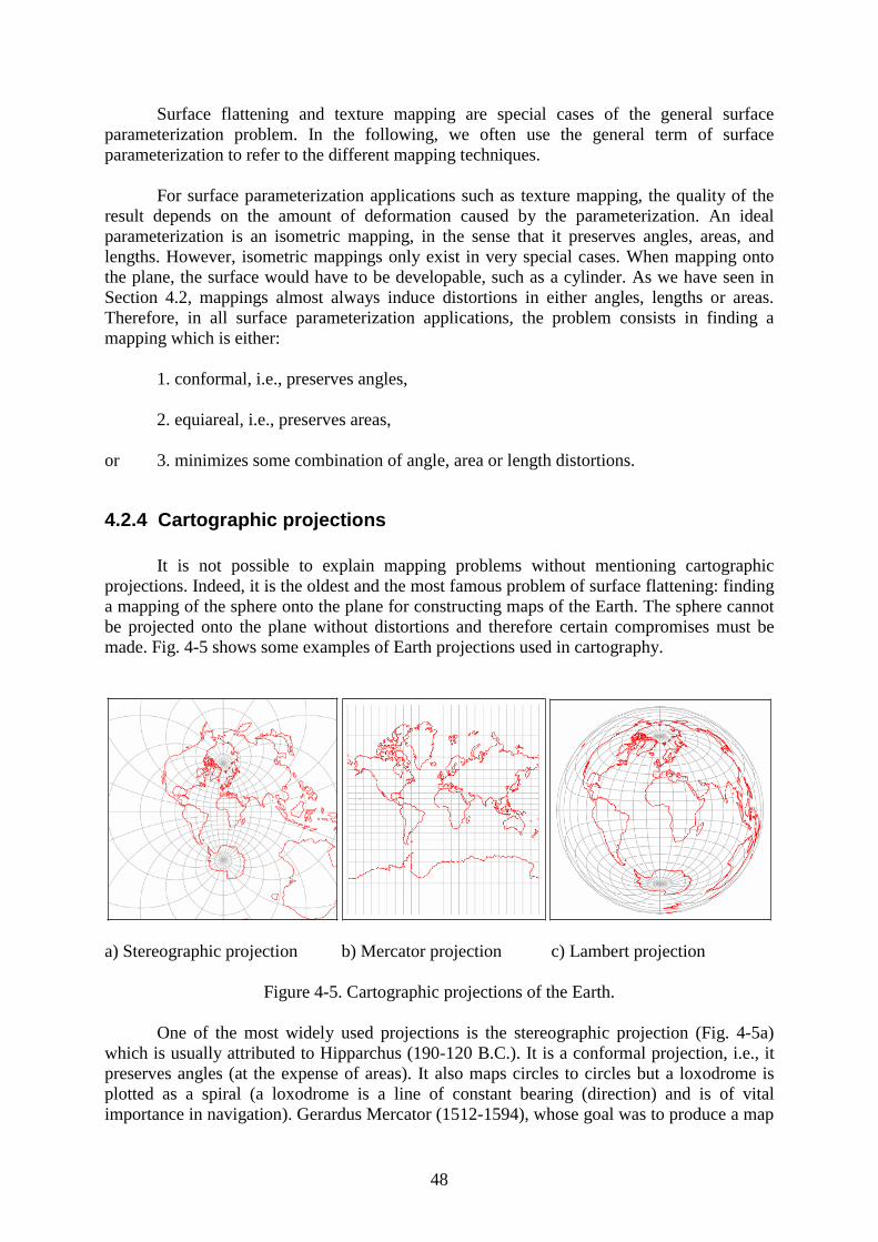
48
Surface flattening and texture mapping are special cases of the general surface parameterization problem. In the following, we often use the general term of surface parameterization to refer to the different mapping techniques.
For surface parameterization applications such as texture mapping, the quality of the result depends on the amount of deformation caused by the parameterization. An ideal parameterization is an isometric mapping, in the sense that it preserves angles, areas, and lengths. However, isometric mappings only exist in very special cases. When mapping onto the plane, the surface would have to be developable, such as a cylinder. As we have seen in Section 4.2, mappings almost always induce distortions in either angles, lengths or areas. Therefore, in all surface parameterization applications, the problem consists in finding a mapping which is either:
1. conformal, i.e., preserves angles,
2. equiareal, i.e., preserves areas,
or 3. minimizes some combination of angle, area or length distortions.
4.2.4 Cartographic projections
It is not possible to explain mapping problems without mentioning cartographic projections. Indeed, it is the oldest and the most famous problem of surface flattening: finding a mapping of the sphere onto the plane for constructing maps of the Earth. The sphere cannot be projected onto the plane without distortions and therefore certain compromises must be made. Fig. 4-5 shows some examples of Earth projections used in cartography.
a) Stereographic projection b) Mercator projection c) Lambert projection
Figure 4-5. Cartographic projections of the Earth.
One of the most widely used projections is the stereographic projection (Fig. 4-5a) which is usually attributed to Hipparchus (190-120 B.C.). It is a conformal projection, i.e., it preserves angles (at the expense of areas). It also maps circles to circles but a loxodrome is plotted as a spiral (a loxodrome is a line of constant bearing (direction) and is of vital importance in navigation). Gerardus Mercator (1512-1594), whose goal was to produce a map
49
which navigators could use to determine courses, created in 1569 the conformal cylindrical Mercator projection (Fig. 4-5b) which draws every loxodrome as a straight line. However, the stereographic and Mercator projections do not preserve areas. Johann Heinrich Lambert (1728-1777) found the first equiareal projection (Fig. 4-5c) in 1772. This projection does not preserve angles.
All these projections can be seen as functions that map a part of the surface of the sphere to a planar domain and the inverse of this mapping is usually called a parameterization.
4.3 Previous work on surface parameterization
As we have seen in the previous sections, surface parameterization always induces some distortions. Therefore, before using a surface parameterization method, one needs to define the desired properties of the mapping according to its application. In Section 4.1, we presented the requirements for our anatomical visualization flattening. Therefore, we present an overview of previous work on this topic in order to find a method which meets these requirements.
Significant research efforts have been made to produce a least distorted flattened surface in the context of texture mapping applications or visualization of textured surfaces extracted from medical volume image. We briefly review the major techniques proposed for surface parameterization. We refer the reader to Floater and Hormann [2004] for a more detailed discussion of the numerous techniques available.
In the context of Magnetic Resonance Images (MRI), Haker et. al. [1999] proposed a technique for flattening the brain surface. They create a quasi-conformal mapping between the surface of interest and a disc. The method has also been applied to the 3D visualization of colon CT images [Haker et. al. 2000]. This method is based on the computation of a harmonic map by minimizing the Dirichlet energy on the flattened surface. To approximate the harmonic map they use the finite elements method. This method of resolution was first introduced to the computer graphics community by Eck et al. [1995] and called simply a discrete harmonic map, although a similar technique had earlier been used by [Pinkall and Polthier 1993]. The main advantage of this method over earlier approaches is that this is a quadratic minimization problem and it reduces to solving a linear system of equations. While this technique minimizes angular distortions, it creates unpredictable metric distortions and therefore may not be used for our application.
Other researchers addressed the problem of surface flattening in the context of texture mapping [Bennis et. al. 1991; Levy and Mallet 1998; Levy et. al. 2002; Sheffer and de Sturler 2001], or in the more general context of parameterization of 3D meshes [Floater 1997; Lee et. al. 1998]. In many approaches the surface is divided into a collection of patches that can be unfolded with little stretch [Sander et. al. 2001; Alliez et. al. 2002; Levy et. al. 2002; Sorkine et. al. 2002]. While stretch is minimized, these approaches create seams between patches and therefore discontinuities. For anatomic surface visualization, surface cuts are problematic, since continuous surface sections are needed in order to provide an understanding of the relationships between the different anatomic structure elements.These methods may be generally adapted to the visualization of flattened surfaces by applying unfolding techniques to the whole surface.
50
There exist many patch unfolding techniques. The classical approach treats the surface unfolding problem as finding the minimum of some functional that measures the difference between the current parameterization and an ideal isometric parameterization [Eck et al. 1995; Floater 1997]. First, the boundary vertices are assigned initial positions (usually on a circle or a square). Then the parameterization for the interior vertices is determined by solving a large linear system or through a nonlinear optimization process. Zigelman et. al. [2001] present a method for globally minimizing distortions based of the preservation of geodesic distances. They compute geodesic distances between each pair of mesh vertices and applying multidimensional scaling in order to optimally preserve these distances on the flattened surface. Levy and Mallet [1998] apply an iterative method for constructing a parameterization of the surface which globally minimizes distortions. This method tries to preserve as much as possible orthogonality and constant spacing between isoparametric curves of the new parameterization. Compared with other global optimization techniques, this method allows the user to specify the region where distortions should be minimized. Sheffer and de Sturler [2001] proposed to use an angle based flattening approach for surface unfolding. This approach measures stretch in term of the angles deficits between the triangles on the surface and their textural images. In [Sheffer et. al. 2005], the authors presented a modified algorithm which ensures the validity of the flattened map and improves computation time. They also showed that the method creates flattened surfaces with low area distortions.
Other stretch metrics have been used for minimizing distortions. Maillot et. al. [1993] have used the Green-Lagrange deformation tensor as stretch measure. Sander et. al. [2001] defined a geometric stretch metric that is based on the average and maximal stretch in all directions of a triangle. Sorkine et. al. [2002] and Khodakovsky et. al. [2003] have devised stretch metrics based on the maximum and minimum eigenvalues of the stretch tensor.
While these methods are efficient in term of global distortions minimization, most of these texture mapping or surface parameterization methods do not provide users with a mean of controlling the distribution of distortions. Moreover, with such techniques it is not possible to specify where distances have to be preserved. In addition, global optimization techniques such as [Eck et. al. 1995; Floater 1997; Sheffer and de Sturler 2001; Levy and Mallet 1998; Zigelman et. al. 2001] require memory and time consuming algorithms in order to solve large linear systems or to carry out an iterative optimization process.
Some works remove the need for a global optimization process or large system solving by using iterative techniques. Bennis et. al. [1991] proposed a simple piecewise surface flattening method for parametric surfaces which iteratively flattens isoparametric curves by preserving their lengths and their geodesic curvature starting from a central reference curve which is flattened without distortions. The geodesic curvature preservation method decreases distortions along flattened curves and distortions are minimized near a central point. A distortion threshold is fixed and cuts on the surface are introduced when this threshold is reached. The cuts are necessary to ensure the validity of the flattening map since self intersections between flattened curves may occur when this algorithm is applied to the whole surface. In a similar approach, Sorkine et. al. [2002] presented a method which iteratively flattens triangles with the minimum of distortion starting from a focus point of interest. As Bennis et. al., cuts are introduced during the process, in order to respect a fixed geometric stretch metric threshold. Therefore, distortions are minimized near the focus point, distortions increase with increasing distance from the focus point and global distortions are under the specified threshold. Mlejnek et. al. [2004] have applied this method to the interactive thickness visualization of articular cartilages with a different stretch metric. The method
51
iteratively flattens triangles starting from a focus point while trying to minimize area distortions.
The algorithms of [Sorkine et. al. 2002] and of [Bennis et. al. 1991] are interesting for our application since these methods meet the requirement of minimizing distortions around a focus point. Moreover, these processes are computationally efficient since the flattening and distortion minimization process is carried out at the same time. However, Sorkine et. al. [2002] do not preserve distances on the surface. In [Sorkine et. al. 2002] or [Mlejneck et. al. 2004] only a focus point where distortions are minimized may be specified but no controls are given on the distortions distribution on the surrounding surface parts. In [Bennis et. al. 1991], distances are preserved along specific curves located on the surface. However, it is not possible to choose the location of these curves. In addition, these unfolding techniques automatically create cuts during the flattening process.
These algorithms may not be used directly in our application. However, we propose to use some of the techniques proposed by Bennis et. al. and the general approach of the two algorithms. First, we propose to use geodesic curvature and distance preservation on a central curve. This provides a simple and fast way to minimize distortions around a band of interest. Second, as in the Bennis et. al. algorithm, we propose to flatten specific curves on the surface with length preservation. In addition, we want to provide users with the possibility to control the location of these curves.
In Chapters 5 and 6, we present the different flattening methods we develop in this work, in order to visualize curved texture surfaces extracted from medical volume images. They are inspired by the algorithm from Bennis et. al.; in particular, they use the geodesic curvature preservation method. Therefore the original algorithm is presented in detail in the following section.
4.4 Bennis et. al. Algorithm and Geodesic Curvature preservation
Let us present the Bennis et. al. parametric surface flattening. The idea of geodesic curvature preservation on which the algorithm is based will be later used in our flattening algorithm. Therefore it seems necessary to recall the main steps of this algorithm.
4.4.1 Outline of the approach.
The surfaces considered here are given by a piecewise parametric representation:
[ ] [ ]max max
( , )
( , ) ( , ) , ( , ) 0, 0,
( , )
x u v
M u v y u v u v u v
z u v
= ∈ × (4-1)
The surface is first regularly sampled into a grid of 3-D points, along the isoparametric curves (in parameters space). The sampling must be refined enough to approximate the arc length between two successive sample points along an isoparametric curve by their Euclidean distance. The main idea of the technique is to map isoparametric curves of the surface onto curves of the plane, with geodesic curvature preservation at sample points and with arc length
52
(i.e. chord length) preservation. Geodesic curves, i.e. curves having null geodesic curvature at each point, behave like straight lines when mapped onto the plane. Instead of mapping onto the plane unknown surface curves which may be difficult to compute such as geodesics, Bennis et al. use already available isoparametric curves and take into account their topological properties in the mapping process.
4.4.2 Curve flattening with arc length and geodesic curvature preservation
In this part we develop the method of geodesic curvature preservation along a surface curve according to the original presentation by [Bennis et. al. 1991].
Let us recall that surface curves are approximated by polylines. A curve C that is to be mapped onto the plane contains 1n + sample points ,iM 0..i n= . Let us denote by iN and
ipT , respectively, the normal vector and the tangent plane to the surface at point iM . The
curve flattening algorithm runs as follows:
1. Map the first curve segment 0 1M M onto a segment 0 1P P in the plane (Oxy) such that
0 1 0 1( ) ( )d M M d P P= , where d designates the Euclidean distance function.
2. For each , 2 , jj j n P≤ ≤ is iteratively computed in the plane as follows:
a) Project jM and 2jM − onto the tangent plane to the surface at 1jM − (see Fig. 4-6).
This provides two points in -1jpT , called jM and 2jM − given by the formulas:
1 -1 -1
2 2 1 2 -1 -1
(( ) )
(( ) )
j j j j j j
j j j j j j
M M M M
M M M M
−
− − − −
= + − ⋅
= + − ⋅
N N
N N (4-2)
b) Use a dilatation in -1jpT , in order to transform jM into a point jM ′ such that
1 1( , ) ( , )j j j jd M M d M M− − ′= (see Fig. 4-6).
11 1
1
( )j j
j j j jj j
M MM M M M
M M
−− −
−
−′ = + −
− (4-3)
c) As 2jP − and 1jP − are already computed, the desired point jP is the point of (Oxy)
that preserves simultaneously the angle 1jθ − between 2 1j jM M− − and 1j jM M− ′ , and
the distance 1( , )j jd M M− ′ .
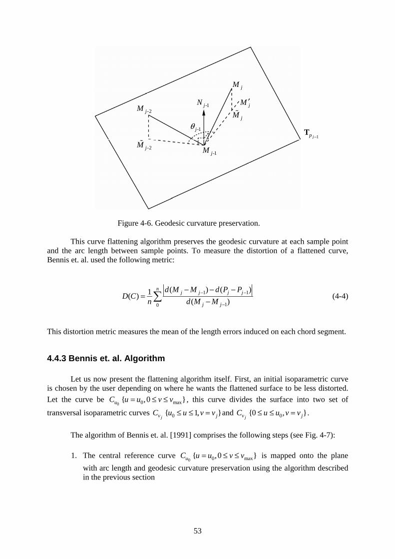
53
Figure 4-6. Geodesic curvature preservation.
This curve flattening algorithm preserves the geodesic curvature at each sample point and the arc length between sample points. To measure the distortion of a flattened curve, Bennis et. al. used the following metric:
1 1
10
( ) ( )1( )( )
nj j j j
j j
d M M d P PD C
n d M M− −
−
− − −=
− (4-4)
This distortion metric measures the mean of the length errors induced on each chord segment.
4.4.3 Bennis et. al. Algorithm
Let us now present the flattening algorithm itself. First, an initial isoparametric curve is chosen by the user depending on where he wants the flattened surface to be less distorted.
Let the curve be 0uC 0 max{ ,0 }u u v v= ≤ ≤ , this curve divides the surface into two set of
transversal isoparametric curves jvC 0{ 1, }ju u v v≤ ≤ = and
jvC 0{0 , }ju u v v≤ ≤ = .
The algorithm of Bennis et. al. [1991] comprises the following steps (see Fig. 4-7):
1. The central reference curve 0uC 0 max{ ,0 }u u v v= ≤ ≤ is mapped onto the plane
with arc length and geodesic curvature preservation using the algorithm described in the previous section
-1jN
1jp −T
-1jM
-2jM
jM
-2jM
jMjM ′
-1jθ
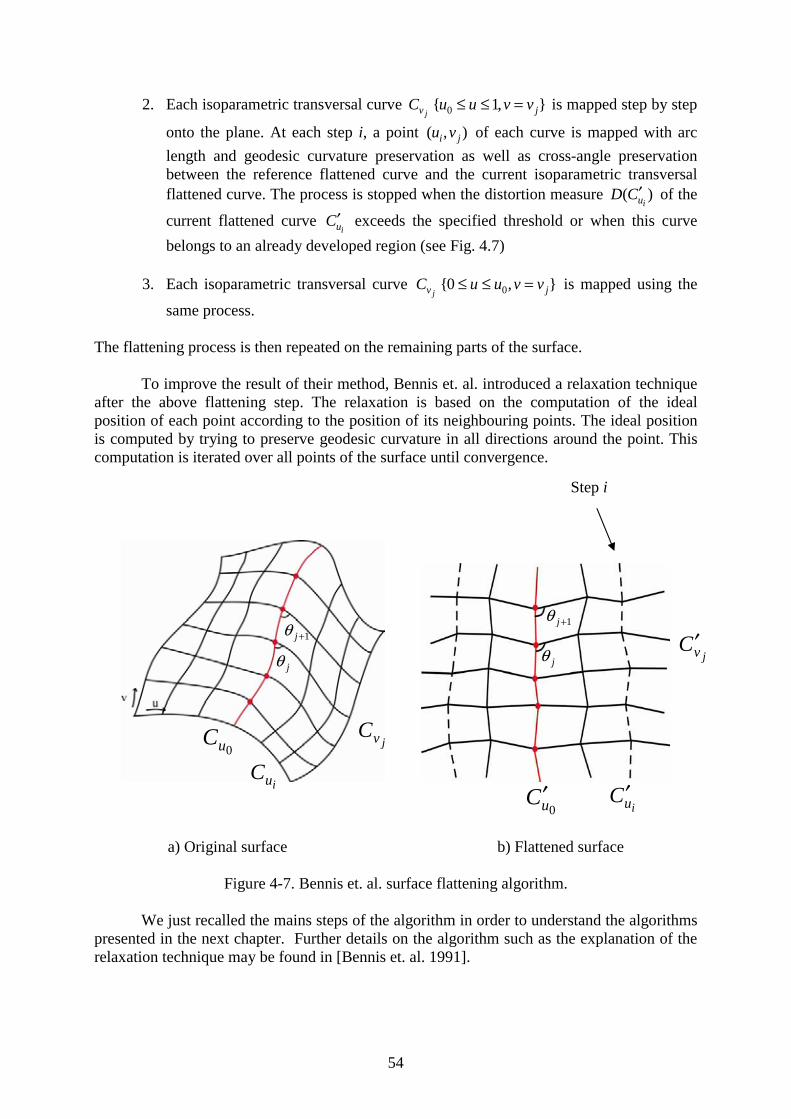
54
2. Each isoparametric transversal curve jvC 0{ 1, }ju u v v≤ ≤ = is mapped step by step
onto the plane. At each step i, a point ( , )i ju v of each curve is mapped with arc
length and geodesic curvature preservation as well as cross-angle preservation between the reference flattened curve and the current isoparametric transversal flattened curve. The process is stopped when the distortion measure ( )
iuD C′ of the
current flattened curve iuC′ exceeds the specified threshold or when this curve
belongs to an already developed region (see Fig. 4.7)
3. Each isoparametric transversal curve jvC 0{0 , }ju u v v≤ ≤ = is mapped using the
same process.
The flattening process is then repeated on the remaining parts of the surface.
To improve the result of their method, Bennis et. al. introduced a relaxation technique after the above flattening step. The relaxation is based on the computation of the ideal position of each point according to the position of its neighbouring points. The ideal position is computed by trying to preserve geodesic curvature in all directions around the point. This computation is iterated over all points of the surface until convergence.
a) Original surface b) Flattened surface
Figure 4-7. Bennis et. al. surface flattening algorithm.
We just recalled the mains steps of the algorithm in order to understand the algorithms presented in the next chapter. Further details on the algorithm such as the explanation of the relaxation technique may be found in [Bennis et. al. 1991].
0uC
iuC
jvC
jθ1jθ +
1jθ +
jθ jvC′
iuC′0uC′
Step i
55
4.6 Conclusion
In this chapter, we described the surface flattening problem and reviewed the principal research works in this domain. We showed that, in the general case, it is not possible to flatten a surface without distortions in terms of angles, lengths or area. Therefore, it is important to decide first which surface properties need to be preserved after the flattening. For our anatomical surface visualization application, we proposed to minimize distortions around a focus point and to provide users with the possibility to carry out distance measurements on the flattened surface. Existing surface parameterization algorithms do not meet these requirements. Therefore, new algorithms need to be proposed. For this purpose, we described an existing algorithm that shows interesting properties which is used in our flattening methods.
The first application of surface parameterization has been cartographic projections. The goal of such projections is to visualize the Earth within a plane and provide the possibility of carrying out measurements on the flattened map. Therefore, several cartographic projections have been proposed, each having its specific properties depending on the kind of application.
We propose to use the same approach in our surface flattening methods. As in the case of cartographic projection, we propose different flattening methods allowing to measure different kinds of distances on the surface. Users may then choose the most adequate method for their application or use both flattening methods for studying the surface.

56
57
5 Distance preserving flattening of surface sections: parallel planes and radial planes flattening
In this chapter we present two different distance preserving flattening algorithms which minimize distortions around a focus point and preserves distances along user specified orientations. The resulting flattened views allow users to carry out measurements on the surface. Thanks to a multiresolution technique, the curved surfaces may be instantly flattened providing user with the possibility to interactively move the focus point and therefore to make a thorough inspection of the surface.
5.1 Introduction
Flattening of ruled and free-form surfaces allows users to precisely inspect curved anatomic structures. While the flattening of a ruled surface is straightforward, flattening of a free-form surface needs to be intuitive, i.e. the user should be able to specify the regions of the surface which should be reproduced with a high fidelity. Moreover, most of the existing surface flattening methods which globally minimize a distortion criterion are computationally expensive. They could not be integrated in an interactive surface extraction and flattening application. For such an application, a fast and simple flattening algorithm is required for ensuring interactivity.
Therefore, in this chapter, we present two different distance preserving surface flattening methods which preserve distances according to user-specified orientations and minimize distortions around a user specified focus point [Saroul et. al. 2006]. For a thorough inspection of a surface, the user may therefore successively select different focus points. The surface flattening methods presented here have similar goals to the methods for cartographic projections. They try to preserve distances along certain orientations and minimize distortions around a point or a curve of interest. They can therefore be seen as an extension of cartographic projections from the sphere to more general curved surfaces.
The first flattening method (Section 5.2) preserves distances along curves located at the intersection between the surface and planes of constant orientation specified by the user. The second algorithm (Section 5.3) preserves distances along curves located within radial planes crossing a center of interest (focus point). These flattening algorithms also minimize the metric and angular distortions in the proximity of the focus point.
We discuss the respective advantages and drawbacks of the two surface flattening methods by comparing their distortion maps (Section 5.4). We also introduce a multiresolution flattening method (Section 5.5) enabling surfaces to be instantly flattened.
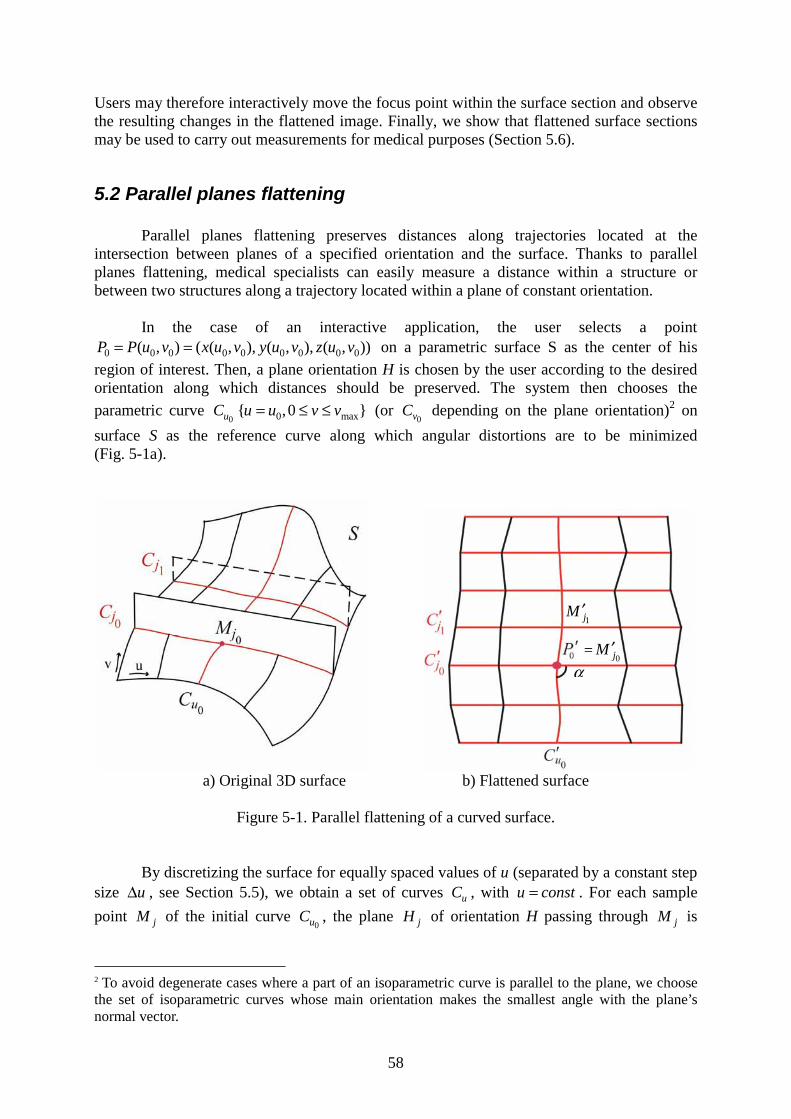
58
Users may therefore interactively move the focus point within the surface section and observe the resulting changes in the flattened image. Finally, we show that flattened surface sections may be used to carry out measurements for medical purposes (Section 5.6).
5.2 Parallel planes flattening
Parallel planes flattening preserves distances along trajectories located at the intersection between planes of a specified orientation and the surface. Thanks to parallel planes flattening, medical specialists can easily measure a distance within a structure or between two structures along a trajectory located within a plane of constant orientation.
In the case of an interactive application, the user selects a point
0 0 0 0 0 0 0 0 0( , ) ( ( , ), ( , ), ( , ))P P u v x u v y u v z u v= = on a parametric surface S as the center of his
region of interest. Then, a plane orientation H is chosen by the user according to the desired orientation along which distances should be preserved. The system then chooses the
parametric curve 0uC 0 max{ ,0 }u u v v= ≤ ≤ (or
0vC depending on the plane orientation)2 on
surface S as the reference curve along which angular distortions are to be minimized (Fig. 5-1a).
a) Original 3D surface b) Flattened surface
Figure 5-1. Parallel flattening of a curved surface.
By discretizing the surface for equally spaced values of u (separated by a constant step size u∆ , see Section 5.5), we obtain a set of curves uC , with u const= . For each sample
point jM of the initial curve 0uC , the plane jH of orientation H passing through jM is
2 To avoid degenerate cases where a part of an isoparametric curve is parallel to the plane, we choose the set of isoparametric curves whose main orientation makes the smallest angle with the plane’s normal vector.
α
1jM ′
=0j
M ′
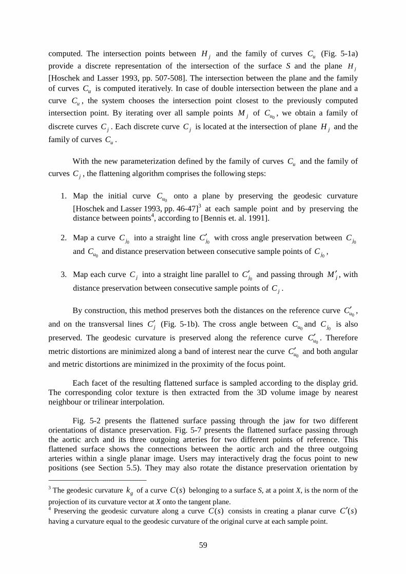
59
computed. The intersection points between jH and the family of curves uC (Fig. 5-1a)
provide a discrete representation of the intersection of the surface S and the plane jH
[Hoschek and Lasser 1993, pp. 507-508]. The intersection between the plane and the family of curves uC is computed iteratively. In case of double intersection between the plane and a
curve uC , the system chooses the intersection point closest to the previously computed
intersection point. By iterating over all sample points jM of 0uC , we obtain a family of
discrete curves jC . Each discrete curve jC is located at the intersection of plane jH and the
family of curves uC .
With the new parameterization defined by the family of curves uC and the family of
curves jC , the flattening algorithm comprises the following steps:
1. Map the initial curve 0uC onto a plane by preserving the geodesic curvature
[Hoschek and Lasser 1993, pp. 46-47]3 at each sample point and by preserving the distance between points4, according to [Bennis et. al. 1991].
2. Map a curve 0j
C into a straight line 0j
C′ with cross angle preservation between 0j
C
and0uC and distance preservation between consecutive sample points of
0jC ,
3. Map each curve jC into a straight line parallel to 0j
C′ and passing through jM ′ , with
distance preservation between consecutive sample points of jC .
By construction, this method preserves both the distances on the reference curve 0uC′ ,
and on the transversal lines jC′ (Fig. 5-1b). The cross angle between 0uC and
0jC is also
preserved. The geodesic curvature is preserved along the reference curve 0uC′ . Therefore
metric distortions are minimized along a band of interest near the curve 0uC′ and both angular
and metric distortions are minimized in the proximity of the focus point.
Each facet of the resulting flattened surface is sampled according to the display grid. The corresponding color texture is then extracted from the 3D volume image by nearest neighbour or trilinear interpolation.
Fig. 5-2 presents the flattened surface passing through the jaw for two different orientations of distance preservation. Fig. 5-7 presents the flattened surface passing through the aortic arch and its three outgoing arteries for two different points of reference. This flattened surface shows the connections between the aortic arch and the three outgoing arteries within a single planar image. Users may interactively drag the focus point to new positions (see Section 5.5). They may also rotate the distance preservation orientation by
3 The geodesic curvature gk of a curve ( )C s belonging to a surface S, at a point X, is the norm of the
projection of its curvature vector at X onto the tangent plane. 4 Preserving the geodesic curvature along a curve ( )C s consists in creating a planar curve ( )C s′having a curvature equal to the geodesic curvature of the original curve at each sample point.
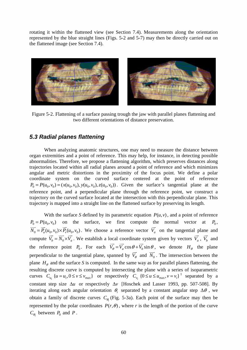
60
rotating it within the flattened view (see Section 7.4). Measurements along the orientation represented by the blue straight lines (Figs. 5-2 and 5-7) may then be directly carried out on the flattened image (see Section 7.4).
Figure 5-2. Flattening of a surface passing trough the jaw with parallel planes flattening and two different orientations of distance preservation.
5.3 Radial planes flattening
When analyzing anatomic structures, one may need to measure the distance between organ extremities and a point of reference. This may help, for instance, in detecting possible abnormalities. Therefore, we propose a flattening algorithm, which preserves distances along trajectories located within all radial planes around a point of reference and which minimizes angular and metric distortions in the proximity of the focus point. We define a polar coordinate system on the curved surface centered at the point of reference
0 0 0 0 0 0 0 0 0( , ) ( ( , ), ( , ), ( , ))P P u v x u v y u v z u v= = . Given the surface’s tangential plane at the
reference point, and a perpendicular plane through the reference point, we construct a trajectory on the curved surface located at the intersection with this perpendicular plane. This trajectory is mapped into a straight line on the flattened surface by preserving its length.
With the surface S defined by its parametric equation ( , )P u v , and a point of reference
0 0 0( , )P P u v= on the surface, we first compute the normal vector at 0P ,
0 0 0 0 0( , ) ( , )u vN P u v P u v= × . We choose a reference vector aV on the tangential plane and
compute 0b aV N V= × . We establish a local coordinate system given by vectors aV , bV and
the reference point 0P . For each cos sina bV V Vθ θ θ= + , we denote Hθ the plane
perpendicular to the tangential plane, spanned by Vθ and 0N . The intersection between the
plane Hθ and the surface S is computed. In the same way as for parallel planes flattening, the
resulting discrete curve is computed by intersecting the plane with a series of isoparametric curves
iuC max{ ,0 }iu u v v= ≤ ≤ or respectively ivC max{0 , }iu u v v≤ ≤ = 1 separated by a
constant step size u∆ or respectively v∆ [Hoschek and Lasser 1993, pp. 507-508]. By iterating along each angular orientation iθ separated by a constant angular step θ∆ , we
obtain a family of discrete curves i
Cθ (Fig. 5-3a). Each point of the surface may then be
represented by the polar coordinates ( , )P r θ , where r is the length of the portion of the curve
iCθ between 0P and P .
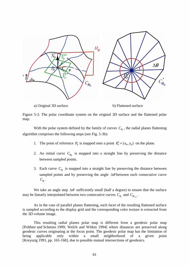
61
a) Original 3D surface b) Flattened surface
Figure 5-3. The polar coordinate system on the original 3D surface and the flattened polar map.
With the polar system defined by the family of curves i
Cθ , the radial planes flattening
algorithm comprises the following steps (see Fig. 5-3b):
1. The point of reference 0P is mapped onto a point 0 0 0( , )P x y′ = on the plane.
2. An initial curve 0
Cθ is mapped into a straight line by preserving the distance
between sampled points.
3. Each curve i
Cθ is mapped into a straight line by preserving the distance between
sampled points and by preserving the angle θ∆ between each consecutive curve
iCθ .
We take an angle step θ∆ sufficiently small (half a degree) to ensure that the surface may be linearly interpolated between two consecutive curves
iCθ and
1iCθ +
.
As in the case of parallel planes flattening, each facet of the resulting flattened surface is sampled according to the display grid and the corresponding color texture is extracted from the 3D volume image.
This resulting radial planes polar map is different from a geodesic polar map [Polthier and Schmies 1999; Welch and Witkin 1994] where distances are preserved along geodesic curves originating at the focus point. The geodesic polar map has the limitation of being applicable only within a small neighborhood of a given point [Kreyszig 1991, pp. 165-168], due to possible mutual intersections of geodesics.
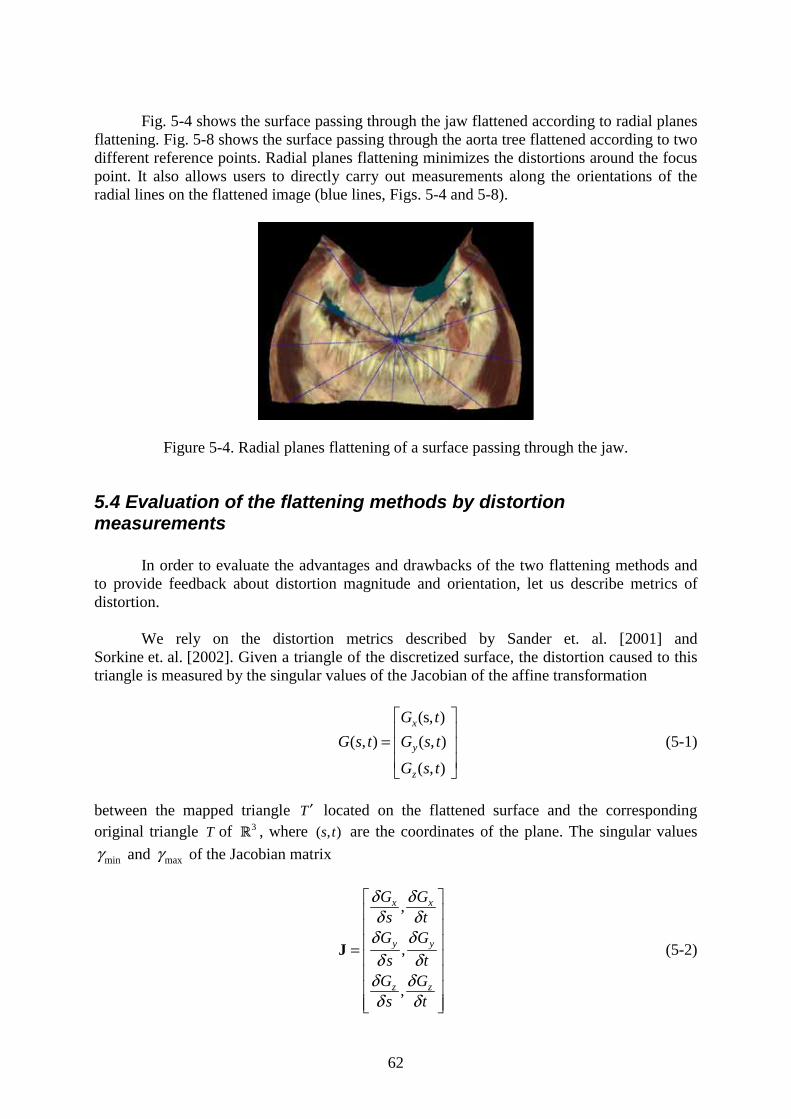
62
Fig. 5-4 shows the surface passing through the jaw flattened according to radial planes flattening. Fig. 5-8 shows the surface passing through the aorta tree flattened according to two different reference points. Radial planes flattening minimizes the distortions around the focus point. It also allows users to directly carry out measurements along the orientations of the radial lines on the flattened image (blue lines, Figs. 5-4 and 5-8).
Figure 5-4. Radial planes flattening of a surface passing through the jaw.
5.4 Evaluation of the flattening methods by distortion measurements
In order to evaluate the advantages and drawbacks of the two flattening methods and to provide feedback about distortion magnitude and orientation, let us describe metrics of distortion.
We rely on the distortion metrics described by Sander et. al. [2001] and Sorkine et. al. [2002]. Given a triangle of the discretized surface, the distortion caused to this triangle is measured by the singular values of the Jacobian of the affine transformation
(s, )
( , ) ( , )
( , )
x
y
z
G t
G s t G s t
G s t
= (5-1)
between the mapped triangle T ′ located on the flattened surface and the corresponding original triangle T of 3 , where ( , )s t are the coordinates of the plane. The singular values
minγ and maxγ of the Jacobian matrix
,
,
,
x x
y y
z z
G Gs t
G G
s tG Gs t
δ δδ δ
δ δδ δ
δ δδ δ
=J (5-2)
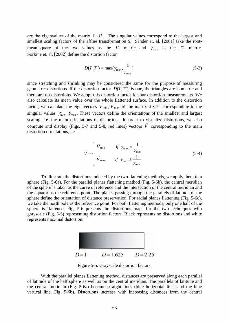
63
are the eigenvalues of the matrix TJ × J . The singular values correspond to the largest and smallest scaling factors of the affine transformation S. Sander et. al. [2001] take the root-
mean-square of the two values as the 2L metric and maxγ as the L∞ metric.
Sorkine et. al. [2002] define the distortion factor
maxmin
1( , ') max( , )D T T γ
γ= (5-3)
since stretching and shrinking may be considered the same for the purpose of measuring geometric distortions. If the distortion factor ( , ')D T T is one, the triangles are isometric and there are no distortions. We adopt this distortion factor for our distortion measurements. We also calculate its mean value over the whole flattened surface. In addition to the distortion
factor, we calculate the eigenvectors min max,V V of the matrix TJ × J corresponding to the
singular values min max,γ γ . These vectors define the orientations of the smallest and largest
scaling, i.e. the main orientations of distortions. In order to visualize distortions, we also
compute and display (Figs. 5-7 and 5-8, red lines) vectors V corresponding to the main distortion orientations, i.e
min maxmin
max maxmin
1
1
V if
VV if
γ γ
γ γ
<=
≥ (5-4)
To illustrate the distortions induced by the two flattening methods, we apply them to a sphere (Fig. 5-6a). For the parallel planes flattening method (Fig. 5-6b), the central meridian of the sphere is taken as the curve of reference and the intersection of the central meridian and the equator as the reference point. The planes passing through the parallels of latitude of the sphere define the orientation of distance preservation. For radial planes flattening (Fig. 5-6c), we take the north pole as the reference point. For both flattening methods, only one half of the sphere is flattened. Fig. 5-6 presents the distortions maps for the two techniques with grayscale (Fig. 5-5) representing distortion factors. Black represents no distortions and white represents maximal distortion.
Figure 5-5. Grayscale distortion factors.
With the parallel planes flattening method, distances are preserved along each parallel of latitude of the half sphere as well as on the central meridian. The parallels of latitude and the central meridian (Fig. 5-6a) become straight lines (blue horizontal lines and the blue vertical line, Fig. 5-6b). Distortions increase with increasing distances from the central
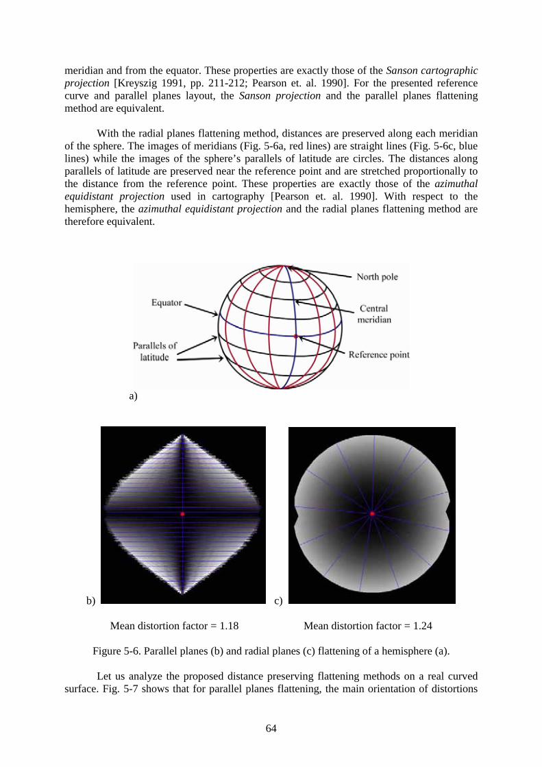
64
meridian and from the equator. These properties are exactly those of the Sanson cartographic projection [Kreyszig 1991, pp. 211-212; Pearson et. al. 1990]. For the presented reference curve and parallel planes layout, the Sanson projection and the parallel planes flattening method are equivalent.
With the radial planes flattening method, distances are preserved along each meridian of the sphere. The images of meridians (Fig. 5-6a, red lines) are straight lines (Fig. 5-6c, blue lines) while the images of the sphere’s parallels of latitude are circles. The distances along parallels of latitude are preserved near the reference point and are stretched proportionally to the distance from the reference point. These properties are exactly those of the azimuthalequidistant projection used in cartography [Pearson et. al. 1990]. With respect to the hemisphere, the azimuthal equidistant projection and the radial planes flattening method are therefore equivalent.
a)
b) c)
Mean distortion factor = 1.18 Mean distortion factor = 1.24
Figure 5-6. Parallel planes (b) and radial planes (c) flattening of a hemisphere (a).
Let us analyze the proposed distance preserving flattening methods on a real curved surface. Fig. 5-7 shows that for parallel planes flattening, the main orientation of distortions
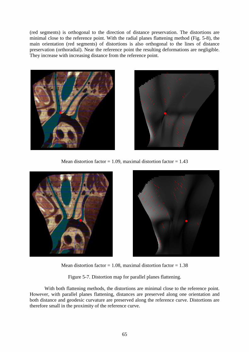
65
(red segments) is orthogonal to the direction of distance preservation. The distortions are minimal close to the reference point. With the radial planes flattening method (Fig. 5-8), the main orientation (red segments) of distortions is also orthogonal to the lines of distance preservation (orthoradial). Near the reference point the resulting deformations are negligible. They increase with increasing distance from the reference point.
Mean distortion factor = 1.09, maximal distortion factor = 1.43
Mean distortion factor = 1.08, maximal distortion factor = 1.38
Figure 5-7. Distortion map for parallel planes flattening.
With both flattening methods, the distortions are minimal close to the reference point. However, with parallel planes flattening, distances are preserved along one orientation and both distance and geodesic curvature are preserved along the reference curve. Distortions are therefore small in the proximity of the reference curve.
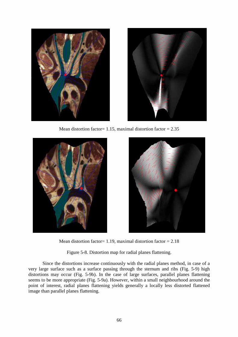
66
Mean distortion factor= 1.15, maximal distortion factor = 2.35
Mean distortion factor= 1.19, maximal distortion factor = 2.18
Figure 5-8. Distortion map for radial planes flattening.
Since the distortions increase continuously with the radial planes method, in case of a very large surface such as a surface passing through the sternum and ribs (Fig. 5-9) high distortions may occur (Fig. 5-9b). In the case of large surfaces, parallel planes flattening seems to be more appropriate (Fig. 5-9a). However, within a small neighbourhood around the point of interest, radial planes flattening yields generally a locally less distorted flattened image than parallel planes flattening.
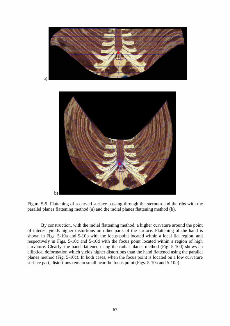
67
a)
b)
Figure 5-9. Flattening of a curved surface passing through the sternum and the ribs with the parallel planes flattening method (a) and the radial planes flattening method (b).
By construction, with the radial flattening method, a higher curvature around the point of interest yields higher distortions on other parts of the surface. Flattening of the hand is shown in Figs. 5-10a and 5-10b with the focus point located within a local flat region, and respectively in Figs. 5-10c and 5-10d with the focus point located within a region of high curvature. Clearly, the hand flattened using the radial planes method (Fig. 5-10d) shows an elliptical deformation which yields higher distortions than the hand flattened using the parallel planes method (Fig. 5-10c). In both cases, when the focus point is located on a low curvature surface part, distortions remain small near the focus point (Figs. 5-10a and 5-10b).
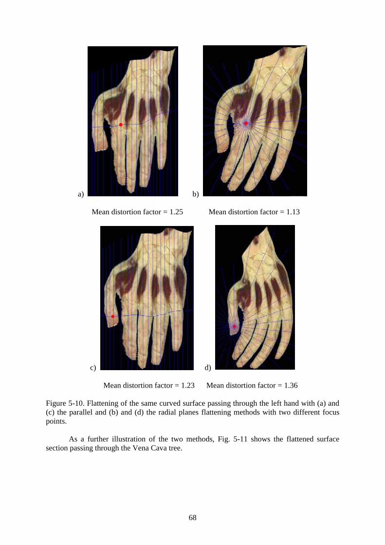
68
a) b)
Mean distortion factor = 1.25 Mean distortion factor = 1.13
c) d)
Mean distortion factor = 1.23 Mean distortion factor = 1.36
Figure 5-10. Flattening of the same curved surface passing through the left hand with (a) and (c) the parallel and (b) and (d) the radial planes flattening methods with two different focus points.
As a further illustration of the two methods, Fig. 5-11 shows the flattened surface section passing through the Vena Cava tree.
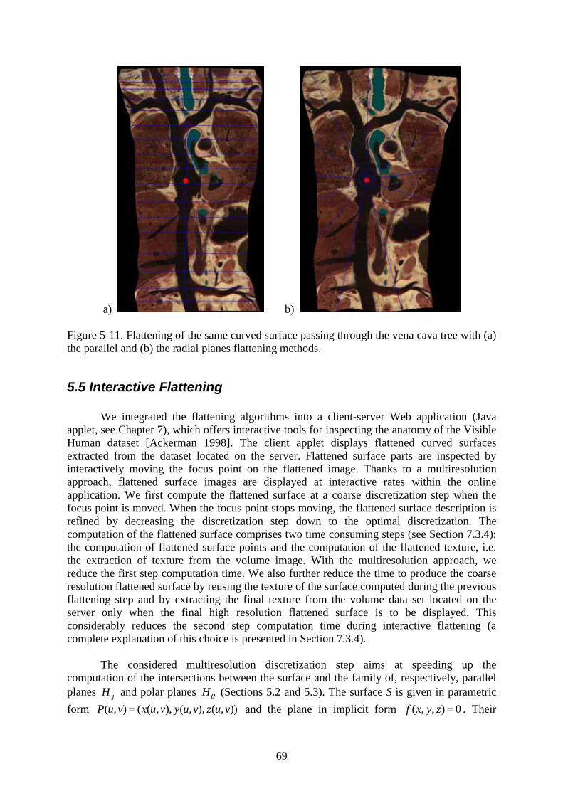
69
a) b)
Figure 5-11. Flattening of the same curved surface passing through the vena cava tree with (a) the parallel and (b) the radial planes flattening methods.
5.5 Interactive Flattening
We integrated the flattening algorithms into a client-server Web application (Java applet, see Chapter 7), which offers interactive tools for inspecting the anatomy of the Visible Human dataset [Ackerman 1998]. The client applet displays flattened curved surfaces extracted from the dataset located on the server. Flattened surface parts are inspected by interactively moving the focus point on the flattened image. Thanks to a multiresolution approach, flattened surface images are displayed at interactive rates within the online application. We first compute the flattened surface at a coarse discretization step when the focus point is moved. When the focus point stops moving, the flattened surface description is refined by decreasing the discretization step down to the optimal discretization. The computation of the flattened surface comprises two time consuming steps (see Section 7.3.4): the computation of flattened surface points and the computation of the flattened texture, i.e. the extraction of texture from the volume image. With the multiresolution approach, we reduce the first step computation time. We also further reduce the time to produce the coarse resolution flattened surface by reusing the texture of the surface computed during the previous flattening step and by extracting the final texture from the volume data set located on the server only when the final high resolution flattened surface is to be displayed. This considerably reduces the second step computation time during interactive flattening (a complete explanation of this choice is presented in Section 7.3.4).
The considered multiresolution discretization step aims at speeding up the computation of the intersections between the surface and the family of, respectively, parallel planes jH and polar planes Hθ (Sections 5.2 and 5.3). The surface S is given in parametric
form ( , ) ( ( , ), ( , ), ( , ))P u v x u v y u v z u v= and the plane in implicit form ( , , ) 0f x y z = . Their
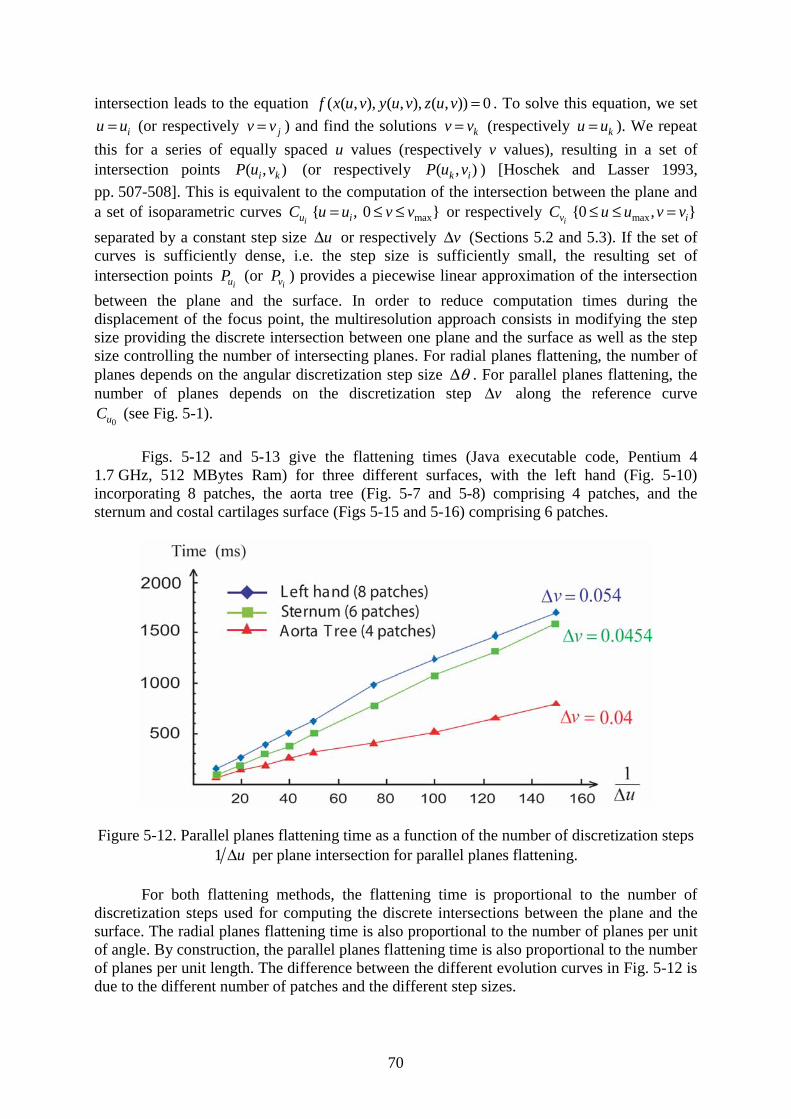
70
intersection leads to the equation ( ( , ), ( , ), ( , )) 0f x u v y u v z u v = . To solve this equation, we set
iu u= (or respectively jv v= ) and find the solutions kv v= (respectively ku u= ). We repeat
this for a series of equally spaced u values (respectively v values), resulting in a set of intersection points ( , )i kP u v (or respectively ( , )k iP u v ) [Hoschek and Lasser 1993,
pp. 507-508]. This is equivalent to the computation of the intersection between the plane and a set of isoparametric curves
iuC max{ , 0 }iu u v v= ≤ ≤ or respectively ivC max{0 , }iu u v v≤ ≤ =
separated by a constant step size u∆ or respectively v∆ (Sections 5.2 and 5.3). If the set of curves is sufficiently dense, i.e. the step size is sufficiently small, the resulting set of intersection points
iuP (or ivP ) provides a piecewise linear approximation of the intersection
between the plane and the surface. In order to reduce computation times during the displacement of the focus point, the multiresolution approach consists in modifying the step size providing the discrete intersection between one plane and the surface as well as the step size controlling the number of intersecting planes. For radial planes flattening, the number of planes depends on the angular discretization step size θ∆ . For parallel planes flattening, the number of planes depends on the discretization step v∆ along the reference curve
0uC (see Fig. 5-1).
Figs. 5-12 and 5-13 give the flattening times (Java executable code, Pentium 4 1.7 GHz, 512 MBytes Ram) for three different surfaces, with the left hand (Fig. 5-10) incorporating 8 patches, the aorta tree (Fig. 5-7 and 5-8) comprising 4 patches, and the sternum and costal cartilages surface (Figs 5-15 and 5-16) comprising 6 patches.
Figure 5-12. Parallel planes flattening time as a function of the number of discretization steps 1 u∆ per plane intersection for parallel planes flattening.
For both flattening methods, the flattening time is proportional to the number of discretization steps used for computing the discrete intersections between the plane and the surface. The radial planes flattening time is also proportional to the number of planes per unit of angle. By construction, the parallel planes flattening time is also proportional to the number of planes per unit length. The difference between the different evolution curves in Fig. 5-12 is due to the different number of patches and the different step sizes.
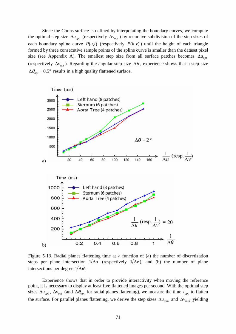
71
Since the Coons surface is defined by interpolating the boundary curves, we compute the optimal step size optu∆ (respectively optv∆ ) by recursive subdivision of the step sizes of
each boundary spline curve ( , )P u i (respectively ( , )P k v ) until the height of each triangle formed by three consecutive sample points of the spline curve is smaller than the dataset pixel size (see Appendix A). The smallest step size from all surface patches becomes optu∆(respectively optv∆ ). Regarding the angular step size θ∆ , experience shows that a step size
0.5optθ∆ = ° results in a high quality flattened surface.
a)
b)
Figure 5-13. Radial planes flattening time as a function of (a) the number of discretization steps per plane intersection 1 u∆ (respectively 1 v∆ ), and (b) the number of plane
intersections per degree 1 θ∆ .
Experience shows that in order to provide interactivity when moving the reference point, it is necessary to display at least five flattened images per second. With the optimal step sizes optu∆ , optv∆ (and optθ∆ for radial planes flattening), we measure the time optt to flatten
the surface. For parallel planes flattening, we derive the step sizes minu∆ and minv∆ yielding
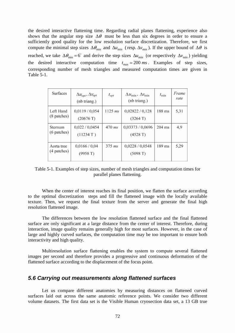
72
the desired interactive flattening time. Regarding radial planes flattening, experience also shows that the angular step size θ∆ must be less than six degrees in order to ensure a sufficiently good quality for the low resolution surface discretization. Therefore, we first compute the minimal step sizes minθ∆ and minu∆ ( minresp. v∆ ). If the upper bound of θ∆ is
reached, we take min 6θ∆ = and derive the step sizes minu∆ (or respectively minv∆ ) yielding
the desired interactive computation time max 200t ms . Examples of step sizes,
corresponding number of mesh triangles and measured computation times are given in Table 5-1.
Table 5-1. Examples of step sizes, number of mesh triangles and computation times for parallel planes flattening.
When the center of interest reaches its final position, we flatten the surface according to the optimal discretization steps and fill the flattened image with the locally available texture. Then, we request the final texture from the server and generate the final high resolution flattened image.
The differences between the low resolution flattened surface and the final flattened surface are only significant at a large distance from the center of interest. Therefore, during interaction, image quality remains generally high for most surfaces. However, in the case of large and highly curved surfaces, the computation time may be too important to ensure both interactivity and high quality.
Multiresolution surface flattening enables the system to compute several flattened images per second and therefore provides a progressive and continuous deformation of the flattened surface according to the displacement of the focus point.
5.6 Carrying out measurements along flattened surfaces
Let us compare different anatomies by measuring distances on flattened curved surfaces laid out across the same anatomic reference points. We consider two different volume datasets. The first data set is the Visible Human cryosection data set, a 13 GB true
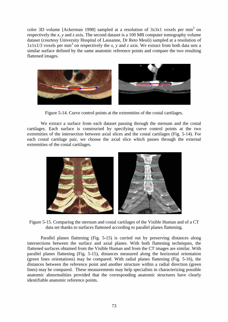
73
color 3D volume [Ackerman 1998] sampled at a resolution of 3x3x1 voxels per mm3 on respectively the x, y and z axis. The second dataset is a 100 MB computer tomography volume dataset (courtesy University Hospital of Lausanne, Dr Reto Meuli) sampled at a resolution of 1x1x1/3 voxels per mm3 on respectively the x, y and z axis. We extract from both data sets a similar surface defined by the same anatomic reference points and compare the two resulting flattened images.
Figure 5-14. Curve control points at the extremities of the costal cartilages.
We extract a surface from each dataset passing through the sternum and the costal cartilages. Each surface is constructed by specifying curve control points at the two extremities of the intersection between axial slices and the costal cartilages (Fig. 5-14). For each costal cartilage pair, we choose the axial slice which passes through the external extremities of the costal cartilages.
Figure 5-15. Comparing the sternum and costal cartilages of the Visible Human and of a CT data set thanks to surfaces flattened according to parallel planes flattening.
Parallel planes flattening (Fig. 5-15) is carried out by preserving distances along intersections between the surface and axial planes. With both flattening techniques, the flattened surfaces obtained from the Visible Human and from the CT images are similar. With parallel planes flattening (Fig. 5-15), distances measured along the horizontal orientation (green lines orientations) may be compared. With radial planes flattening (Fig. 5-16), the distances between the reference point and another structure within a radial direction (green lines) may be compared. These measurements may help specialists in characterizing possible anatomic abnormalities provided that the corresponding anatomic structures have clearly identifiable anatomic reference points.
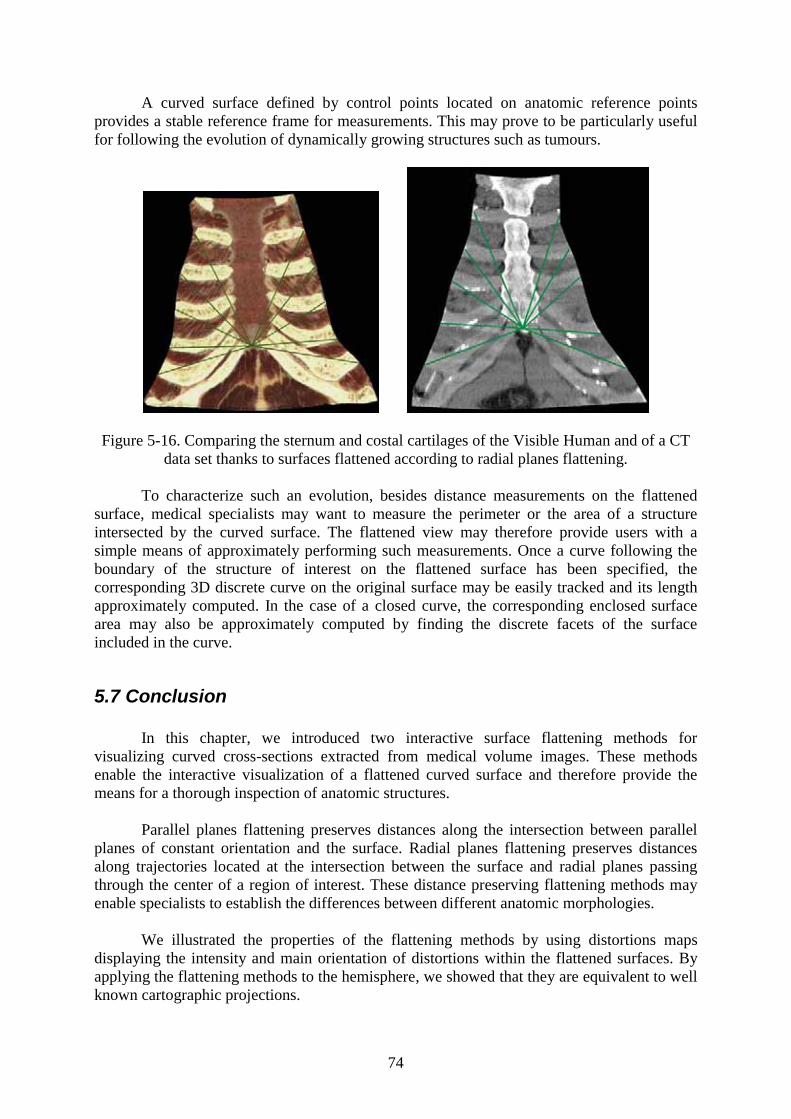
74
A curved surface defined by control points located on anatomic reference points provides a stable reference frame for measurements. This may prove to be particularly useful for following the evolution of dynamically growing structures such as tumours.
Figure 5-16. Comparing the sternum and costal cartilages of the Visible Human and of a CT data set thanks to surfaces flattened according to radial planes flattening.
To characterize such an evolution, besides distance measurements on the flattened surface, medical specialists may want to measure the perimeter or the area of a structure intersected by the curved surface. The flattened view may therefore provide users with a simple means of approximately performing such measurements. Once a curve following the boundary of the structure of interest on the flattened surface has been specified, the corresponding 3D discrete curve on the original surface may be easily tracked and its length approximately computed. In the case of a closed curve, the corresponding enclosed surface area may also be approximately computed by finding the discrete facets of the surface included in the curve.
5.7 Conclusion
In this chapter, we introduced two interactive surface flattening methods for visualizing curved cross-sections extracted from medical volume images. These methods enable the interactive visualization of a flattened curved surface and therefore provide the means for a thorough inspection of anatomic structures.
Parallel planes flattening preserves distances along the intersection between parallel planes of constant orientation and the surface. Radial planes flattening preserves distances along trajectories located at the intersection between the surface and radial planes passing through the center of a region of interest. These distance preserving flattening methods may enable specialists to establish the differences between different anatomic morphologies.
We illustrated the properties of the flattening methods by using distortions maps displaying the intensity and main orientation of distortions within the flattened surfaces. By applying the flattening methods to the hemisphere, we showed that they are equivalent to well known cartographic projections.

75
The two proposed flattening methods minimize geometric distortions around the center of a region of interest located on the surface. In addition, parallel planes flattening also minimizes distortions along a reference curve interpolating between surface patch boundary curves. Thanks to a multiresolution approach, surfaces are flattened at interactive rates, thereby enabling the real time displacement of the center of interest. Users may inspect the different surface parts without noticeable local distortions by displacing the reference point and observe the continuous deformation of the flattened surface.
The presented methods may provide medical specialists with new tools for visualizing and analyzing anatomic structures. They may use them for comparing morphologies or to inspect anatomic structures of patients. Distance measurements carried out on flattened surfaces may also help in detecting anatomic abnormalities.

76
77
6 Optimal parallel planes flattening
In this chapter we extend parallel planes flattening by computing the optimal plane orientation minimizing the resulting distortions on the flattened surface. The method relies on the minimization of the cumulated geodesic curvature along intersections curves. We show that this optimal plane orientation can be computed using a principal component analysis. After studying the efficiency of this algorithm, we apply it to the interactive visualization of anatomic structures.
6.1 Introduction
The parallel planes flattening algorithm presented in the last chapter gives the user the freedom to choose the orientation of the planes intersecting the surface, i.e. the orientation along which distances are preserved. However, the different orientations do not produce the same amount of global distortions on the resulting flattened surface. If the user is interested in getting the least distorted view, it is necessary to determine the planes orientation that produces the smallest distortions on the flattened surface. In the present chapter, we propose a fast and simple algorithm which produces a flattened surface with low distortions and at the same time allows interactive flattening. The method relies on the calculation of an optimal plane orientation which minimizes the cumulated geodesic curvature along intersections between parallel planes and the surface. Finding the optimal plane orientation leading to the least cumulated geodesic curvature along intersection curves can be reduced to a principal component analysis problem. We verify the quality of the method by applying it to representative curved surfaces and by qualitatively and quantitatively comparing the results with those obtained with an existing surface flattening method. Optimal orientation for parallel planes flattening is also applied to the interactive visualization of anatomic structures.
In Section 6.2, we present the concept of geodesic curvature minimization. In Section 6.3, we show that the plane orientation which minimizes the geodesic curvature can be determined through a principal component analysis. In Section 6.4, we apply the method to representative curved surfaces and compare flattened surfaces and their distortion maps to those produced by the parametric surface flattening method introduced by Bennis et. al. [1991]. In Section 6.5, we apply optimal parallel planes flattening for the visualization of curved anatomic surfaces and in Section 6.6, we extend the method for the interactive visualization of a region of interest.
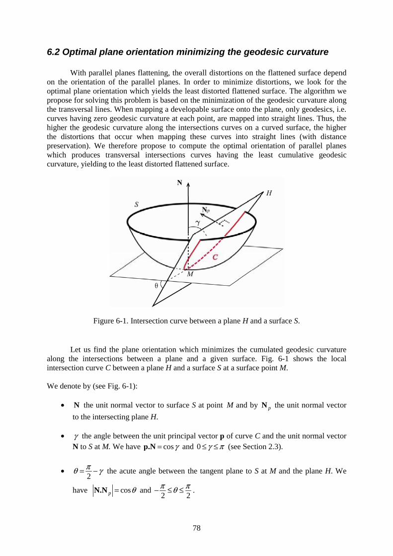
78
6.2 Optimal plane orientation minimizing the geodesic curvature
With parallel planes flattening, the overall distortions on the flattened surface depend on the orientation of the parallel planes. In order to minimize distortions, we look for the optimal plane orientation which yields the least distorted flattened surface. The algorithm we propose for solving this problem is based on the minimization of the geodesic curvature along the transversal lines. When mapping a developable surface onto the plane, only geodesics, i.e. curves having zero geodesic curvature at each point, are mapped into straight lines. Thus, the higher the geodesic curvature along the intersections curves on a curved surface, the higher the distortions that occur when mapping these curves into straight lines (with distance preservation). We therefore propose to compute the optimal orientation of parallel planes which produces transversal intersections curves having the least cumulative geodesic curvature, yielding to the least distorted flattened surface.
Figure 6-1. Intersection curve between a plane H and a surface S.
Let us find the plane orientation which minimizes the cumulated geodesic curvature along the intersections between a plane and a given surface. Fig. 6-1 shows the local intersection curve C between a plane H and a surface S at a surface point M.
We denote by (see Fig. 6-1):
• N the unit normal vector to surface S at point M and by pN the unit normal vector
to the intersecting plane H.
• γ the angle between the unit principal vector p of curve C and the unit normal vector N to S at M. We have cosγ=p.N and 0 γ π≤ ≤ (see Section 2.3).
•2πθ γ= − the acute angle between the tangent plane to S at M and the plane H. We
have cosp θ=N.N and 2 2π πθ− ≤ ≤ .
79
According to formula (2.14) in Section 2.3, for any plane H and any point M,
1 2cosnk k k kγ≤ = ≤ (6-1)
Then,
1 20 cos max( , )k k kγ≤ ≤ (6-2)
And finally, considering the absolute value of the geodesic curvature singk k γ= , we have
1 20 max( , ) tangk k k γ≤ ≤ (6-3)
Therefore, by minimizing tanγ at M, we minimize the geodesic curvature of the
intersection curve C at point M. Minimizing tanγ is equivalent to minimizing sin cosγ θ= .
Thus, by minimizing cosp θ=N.N at point M, we minimize the geodesic curvature at M.
In order to decrease the overall geodesic curvature along all intersection curves jC
(see Section 5.2), we look for a plane orientation which minimizes the sum of the geodesic curvatures. We solve this problem numerically, by discretizing the surface into a set of points
{ }1i i nM ≤ ≤ and minimizing the scalar product pN.N in the least square sense, i.e. by
minimizing 2
1
( )n
i pi
F=
= N .N , where iN is the normal vector at iM . This minimization
method gives the same weight to all normal vectors independently of the local geometry of the surface at point iM and independently of the values of the principal curvatures 1k and 2k .
If 1k and 2k are null at a point iM , the surface is locally planar. In this case the geodesic
curvature of the intersection curve between the surface and the plane at iM is null whatever
the value of i pN .N . Moreover, given a value of i pN .N at a point M, the larger 1k and 2k
are at this point (region of high curvature), the larger the geodesic curvature gk will be at this
point. It therefore makes sense to give more weight to the more curved surface regions in order to decrease the overall geodesic curvature. In order to take these considerations into account, we introduce a weighting factor to the normal vector iN at iM , which depends on
the principal curvature values 1k and 2k .
The mean curvature 1 2
2k k
H+= and the Gaussian curvature 1 2K k k= cannot be used
as weighting factors since their values may be null when the surface is not planar5. According to our experiments, the weighting factor that seems the most appropriate is
2 21 2rmsp k k k= = + , the root mean square curvature, called curvedness of the surface at point
M (introduced in Section 2.3). The curvedness of the surface, also used in [Koenderink and
5 H is null when 1 0k < , 2 0k > and 1k = 2k ; K is null when one of the principal curvatures
is null.
80
Van Doorn 1992] and [Wang et. al. 2003], describes the flatness of the surface independently of its shape (hyperbolic or elliptic region). Planar regions have zero curvedness while highly curved regions have a large curvedness. When introducing the curvedness as weighting factor, the plane orientation optimization problem consists in finding the plane normal vector pN
which minimizes 2 2
1
( . )M
i i pi
F p=
= N N . We present in Section 6.4 examples where curvedness
weighting factors improve the results.
6.3 Minimizing the overall geodesic curvature by principal component analysis
In this section, we develop the equations for calculating the plane normal vector minimizing the overall geodesic curvature over a given surface.
In order to find the optimal normal vector, we discretize the surface S into a set of points { }1i i n
M ≤ ≤ and search for the normal vector pN which minimizes the sum
2
1
( )n
i pi
F=
= N .N , with ( , ) ( , )
( , )( , ) ( , )
u i i v i ii i i
u i i v i i
u v u vu v
u v u v×= =×
P PN N
P Pbeing the normal vector to the
surface S at ( , )i i iM P u v= .
The minimization of F is equivalent to a principal component analysis problem. Indeed, minimizing F according to pN is equivalent to finding a projection axis such that the
sum of the square norms of the projected vectors iN is minimal.
Let { }1i i nN ≤ ≤ be the set of normal vectors seen as points in 3 . Let Hi be the
projection of a point iN onto an axis spanned by unit vector u. Let p=u N be the vector
which minimizes F. u is the orientation of the axis where the sum 2 2 2( . ) ( . )i i i
i i i
F OH ON= = =u u N is minimal.
Let
11 12 13
1 2 3
1 2 3
. . .
i i i
n n n
N N N
N N N
N N N
=A be the 3n× matrix containing the coordinates of points
{ }1i i nN ≤ ≤ and
a
b
c
=u be a unit vector. We denote by TA the transposed matrix of A and by
Tu the transposed vector of u. The element i of the matrix product Au is equal
to1 2 3i i i iaN bN cN+ + = N .u and the product
2T T =u A Au Au is equal to the sum of the
square norms of the projections of points iN onto the u axis 2
1
M
ii
F OH=
= .
81
Therefore, we need to find the vector u minimizing the function
T TF = u A Au under the constraint Tu u = 1 (6-4)
With the method of Lagrange multipliers [Spiegel 1963], we obtain the Lagrangian f1(u) of the system (7)
1 ( ) ( 1).T T Tf λ= − −u u A Au u u
By solving the equation 1( )0
fδδ =u
u, we obtain
2 2 0T λ− =A Au u ,
which is equivalent toT λ=A Au u . (6-5)
Since 0T λ− =A A I u , u is an eigenvector of the matrix TA A . The multiplication of (6-5)
by Tu gives
T T Tλ=u A Au u u ,
and therefore,
T T λ=u A Au . (6-6)
The expected minimal sum F is therefore an eigenvalue of TA A and u is the eigenvector associated with the smallest eigenvalue λ1 of the symmetric matrix TA A .
In the above derivation, all the normal vectors have the same unit weight. When
considering different weighting factors ip , the sum to minimize becomes 2 2
1
( . )M
i p ii
F p=
= N N .
We simply have to replace in the matrix A the vectors iN by the vectors i ip N .
Obtaining the smallest eigenvalue 1λ of TA A requires finding the root of the
characteristic polynomial of TA A of degree 3, i.e. det( ) 0T λ− =A A I , where I is the 3x3
identity matrix [Ralston and Rabinowitz 1978]. Solving Eq. (6-5) for the eigenvector 1u
having the smallest eigenvalue 1λ yields the optimal plane normal vector 1p =N u .
82
6.4 Optimal parallel planes flattening of curved surfaces
6.4.1 Distortions of optimally flattened surfaces
In this section, we evaluate the proposed optimal parallel planes flattening by applying it to several representative surfaces (Fig. 6-2). Let 1 2 3( , , )u u u be the unit eigenvectors of the
matrix TA A with the corresponding eigenvalues 1 2 3, ,λ λ λ with 1 2 3λ λ λ≤ ≤ 6
. We show the
evolution of the distortions by considering plane orientations whose normal vector orientation Np varies within the 1 2( , )u u plane and within the 1 3( , )u u plane.
We still rely on the distortion metric presented in Section 5.4. For the sake of completeness, let us briefly recall it. Given a triangle of the discretized surface, the distortion caused to this triangle is measured by the distortion factor
maxmin
1( , ') max( , )D T T γ
γ= (6-7)
where minγ and maxγ are the singular values of the Jacobian of the affine transformation
which maps triangle T ′ located on the flattened surface onto the corresponding original triangle T .
For each triangle of the flattened surface this distortion factor is calculated. The average distortion is calculated over the whole surface by weighting triangle distortion factors by the corresponding triangle area. For all flattened surfaces, the focus point is chosen at the center of the surface, i.e. 0 0 0( 0.5, 0.5)P P u v= = = .
First, we test optimal parallel planes flattening on a ruled surface ( , ) ( ) 100 P u v s u v= + q defined by a curve ( )s u located in the (xy) plane and a ruling vector q
parallel to the z axis (Fig. 6-2a). A ruled surface is a developable surface, i.e. it can be mapped onto the plane without distortions.
When applying parallel planes flattening to this surface, the optimal plane should be a plane orthogonal to its ruling vector or a plane which contains its ruling vector. The optimal plane computation for this surface gives 1 0.0λ = as the smallest eigenvalue and the
corresponding eigenvector 1 (0,0, 1.0)= −u . This means that the optimal plane’s normal vector
1p =N u is parallel to the ruling vector q. Since the corresponding eigenvalue 1λ is null, the
sum F is also null, i.e. the scalar product pN.N is null for each point of the surface. By
applying parallel planes flattening to this ruled surface, with the optimal plane orientation 1p =N u , we verify that, as expected, the average distortion is equal to one, i.e. the
surface is mapped on to the plane without distortions. In the special case of a ruled surface, there are other plane orientations for which the distortions are null but these orientations do not minimize F 7.
6 If 1 2λ λ= , the system chooses the first computed eigenvector as the optimal eigenvector. 7 For example, any sectional plane containing the ruling vector induces a null geodesic curvature along all intersection curves.
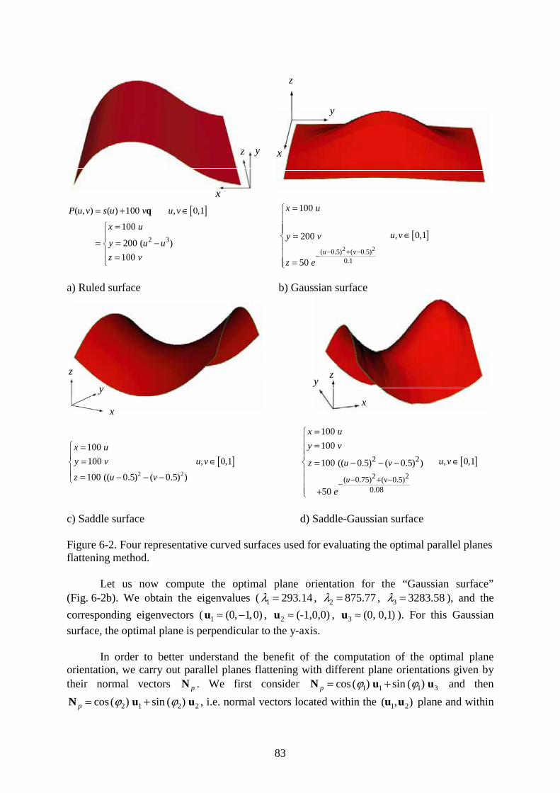
83
[ ]
2 3
( , ) ( ) 100 , 0,1
100
200 ( )
100
P u v s u v u v
x u
y u u
z v
= + ∈
=
= = −=
q
[ ]2 2( 0.5) ( 0.5)0.1
100
, 0,1200
50u v
x u
u vy v
z e− + −−
=
∈=
=
a) Ruled surface b) Gaussian surface
[ ]2 2
100
100 , 0,1
100 (( 0.5) ( 0.5) )
x u
y v u v
z u v
== ∈
= − − −[ ]
2 2
2 2
( 0.75) ( 0.5)0.08
100
100
, 0,1100 (( 0.5) ( 0.5) )
50 u v
x u
y v
u vz u v
e− + −−
==
∈= − − −
+
c) Saddle surface d) Saddle-Gaussian surface
Figure 6-2. Four representative curved surfaces used for evaluating the optimal parallel planes flattening method.
Let us now compute the optimal plane orientation for the “Gaussian surface” (Fig. 6-2b). We obtain the eigenvalues ( 1 293.14λ = , 2 875.77λ = , 3 3283.58λ = ), and the
corresponding eigenvectors ( 1 (0, 1,0)≈ −u , 2 (-1,0,0)≈u , 3 (0, 0,1)≈u ). For this Gaussian
surface, the optimal plane is perpendicular to the y-axis.
In order to better understand the benefit of the computation of the optimal plane orientation, we carry out parallel planes flattening with different plane orientations given by their normal vectors pN . We first consider 1 1 1 3cos ( ) sin ( ) p ϕ ϕ= +N u u and then
2 1 2 2cos ( ) sin ( ) p ϕ ϕ= +N u u , i.e. normal vectors located within the 1 2( , )u u plane and within
x
x
xx
y
zy
z
y
z
y z
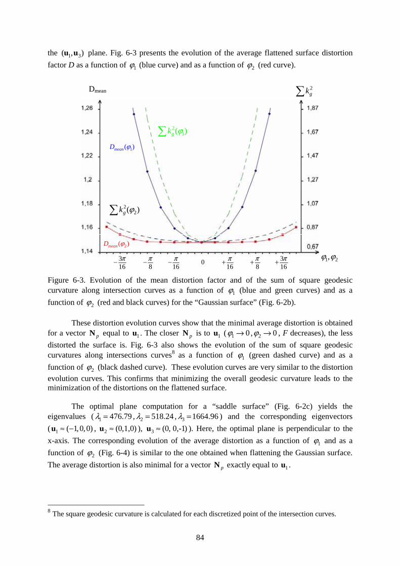
84
the 1 3( , )u u plane. Fig. 6-3 presents the evolution of the average flattened surface distortion
factor D as a function of 1ϕ (blue curve) and as a function of 2ϕ (red curve).
Figure 6-3. Evolution of the mean distortion factor and of the sum of square geodesic curvature along intersection curves as a function of 1ϕ (blue and green curves) and as a
function of 2ϕ (red and black curves) for the “Gaussian surface” (Fig. 6-2b).
These distortion evolution curves show that the minimal average distortion is obtained for a vector pN equal to 1u . The closer pN is to 1u ( 1 0ϕ → , 2 0ϕ → , F decreases), the less
distorted the surface is. Fig. 6-3 also shows the evolution of the sum of square geodesic curvatures along intersections curves8 as a function of 1ϕ (green dashed curve) and as a
function of 2ϕ (black dashed curve). These evolution curves are very similar to the distortion
evolution curves. This confirms that minimizing the overall geodesic curvature leads to the minimization of the distortions on the flattened surface.
The optimal plane computation for a “saddle surface” (Fig. 6-2c) yields the eigenvalues ( 1 476.79λ = , 2 518.24λ = , 3 1664.96λ = ) and the corresponding eigenvectors
( 1 ( 1,0,0)≈ −u , 2 (0,1,0)≈u ), 3 (0, 0,-1)≈u ). Here, the optimal plane is perpendicular to the
x-axis. The corresponding evolution of the average distortion as a function of 1ϕ and as a
function of 2ϕ (Fig. 6-4) is similar to the one obtained when flattening the Gaussian surface.
The average distortion is also minimal for a vector pN exactly equal to 1u .
8 The square geodesic curvature is calculated for each discretized point of the intersection curves.
1( ) meanD ϕ
2( )meanD ϕ
Dmean
1 2,ϕ ϕ316π−
8π−
16π− 0
16π+
8π+ 3
16π+
2gk
21( ) gk ϕ
22( )gk ϕ
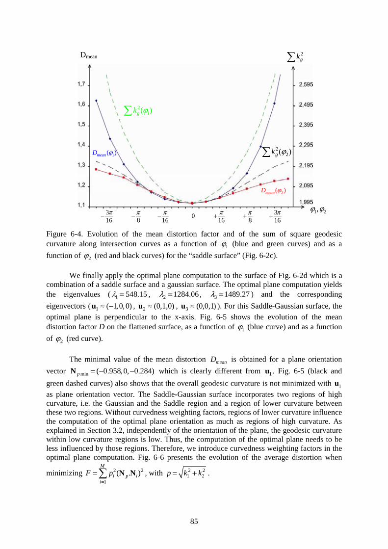
85
Figure 6-4. Evolution of the mean distortion factor and of the sum of square geodesic curvature along intersection curves as a function of 1ϕ (blue and green curves) and as a
function of 2ϕ (red and black curves) for the “saddle surface” (Fig. 6-2c).
We finally apply the optimal plane computation to the surface of Fig. 6-2d which is a combination of a saddle surface and a gaussian surface. The optimal plane computation yields the eigenvalues ( 1 548.15λ = , 2 1284.06λ = , 3 1489.27λ = ) and the corresponding
eigenvectors ( 1 ( 1,0,0)≈ −u , 2 (0,1,0)≈u , 3 (0,0,1)≈u ). For this Saddle-Gaussian surface, the
optimal plane is perpendicular to the x-axis. Fig. 6-5 shows the evolution of the mean distortion factor D on the flattened surface, as a function of 1ϕ (blue curve) and as a function
of 2ϕ (red curve).
The minimal value of the mean distortion meanD is obtained for a plane orientation
vector min ( 0.958,0, 0.284)p = − −N which is clearly different from 1u . Fig. 6-5 (black and
green dashed curves) also shows that the overall geodesic curvature is not minimized with 1uas plane orientation vector. The Saddle-Gaussian surface incorporates two regions of high curvature, i.e. the Gaussian and the Saddle region and a region of lower curvature between these two regions. Without curvedness weighting factors, regions of lower curvature influence the computation of the optimal plane orientation as much as regions of high curvature. As explained in Section 3.2, independently of the orientation of the plane, the geodesic curvature within low curvature regions is low. Thus, the computation of the optimal plane needs to be less influenced by those regions. Therefore, we introduce curvedness weighting factors in the optimal plane computation. Fig. 6-6 presents the evolution of the average distortion when
minimizing 2 2
1
( . )M
i p ii
F p=
= N N , with 2 21 2p k k= + .
Dmean
316π−
8π−
16π− 0
16π+
8π+ 3
16π+
1 2,ϕ ϕ
2gk
21( ) gk ϕ
1( ) meanD ϕ
2( )meanD ϕ
22( )gk ϕ
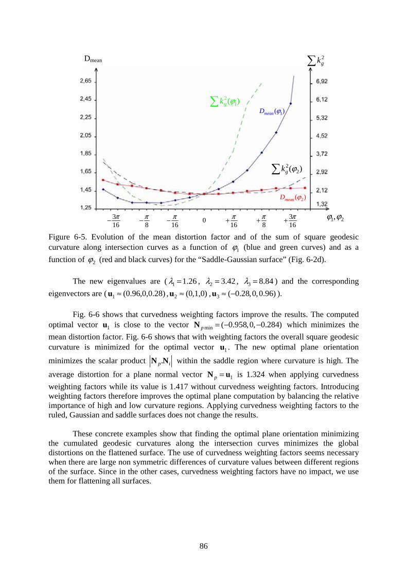
86
Figure 6-5. Evolution of the mean distortion factor and of the sum of square geodesic curvature along intersection curves as a function of 1ϕ (blue and green curves) and as a
function of 2ϕ (red and black curves) for the “Saddle-Gaussian surface” (Fig. 6-2d).
The new eigenvalues are ( 1 1.26λ = , 2 3.42λ = , 3 8.84λ = ) and the corresponding
eigenvectors are ( 1 (0.96,0,0.28)≈u , 2 (0,1,0)≈u , 3 ( 0.28,0,0.96)≈ −u ).
Fig. 6-6 shows that curvedness weighting factors improve the results. The computed optimal vector 1u is close to the vector min ( 0.958,0, 0.284)p = − −N which minimizes the
mean distortion factor. Fig. 6-6 shows that with weighting factors the overall square geodesic curvature is minimized for the optimal vector 1u . The new optimal plane orientation
minimizes the scalar product .p iN N within the saddle region where curvature is high. The
average distortion for a plane normal vector 1p =N u is 1.324 when applying curvedness
weighting factors while its value is 1.417 without curvedness weighting factors. Introducing weighting factors therefore improves the optimal plane computation by balancing the relative importance of high and low curvature regions. Applying curvedness weighting factors to the ruled, Gaussian and saddle surfaces does not change the results.
These concrete examples show that finding the optimal plane orientation minimizing the cumulated geodesic curvatures along the intersection curves minimizes the global distortions on the flattened surface. The use of curvedness weighting factors seems necessary when there are large non symmetric differences of curvature values between different regions of the surface. Since in the other cases, curvedness weighting factors have no impact, we use them for flattening all surfaces.
1 2,ϕ ϕ
2gk
316π−
8π−
16π− 0
16π+
8π+ 3
16π+
21( ) gk ϕ
1( ) meanD ϕ
2( )meanD ϕ
22( )gk ϕ
Dmean
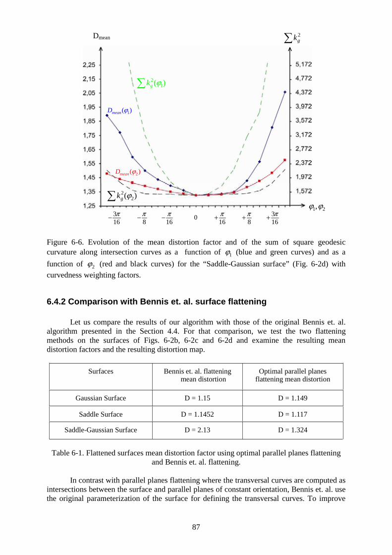
87
Figure 6-6. Evolution of the mean distortion factor and of the sum of square geodesic curvature along intersection curves as a function of 1ϕ (blue and green curves) and as a
function of 2ϕ (red and black curves) for the “Saddle-Gaussian surface” (Fig. 6-2d) with
curvedness weighting factors.
6.4.2 Comparison with Bennis et. al. surface flattening
Let us compare the results of our algorithm with those of the original Bennis et. al. algorithm presented in the Section 4.4. For that comparison, we test the two flattening methods on the surfaces of Figs. 6-2b, 6-2c and 6-2d and examine the resulting mean distortion factors and the resulting distortion map.
Table 6-1. Flattened surfaces mean distortion factor using optimal parallel planes flattening and Bennis et. al. flattening.
In contrast with parallel planes flattening where the transversal curves are computed as intersections between the surface and parallel planes of constant orientation, Bennis et. al. use the original parameterization of the surface for defining the transversal curves. To improve
Surfaces Bennis et. al. flattening mean distortion
Optimal parallel planes flattening mean distortion
Gaussian Surface D = 1.15 D = 1.149
Saddle Surface D = 1.1452 D = 1.117
Saddle-Gaussian Surface D = 2.13 D = 1.324
316π−
8π−
16π− 0
16π+
8π+ 3
16π+
1 2,ϕ ϕ
2gk
21( ) gk ϕ
1( ) meanD ϕ
2( )meanD ϕ
22( )gk ϕ
Dmean
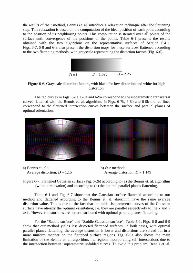
88
the results of their method, Bennis et. al. introduce a relaxation technique after the flattening step. This relaxation is based on the computation of the ideal position of each point according to the position of its neighboring points. This computation is iterated over all points of the surface until convergence of the positions of the points. Table 6-1 presents the results obtained with the two algorithms on the representative surfaces of Section 6.4.1. Figs. 6-7, 6-8 and 6-9 also present the distortion maps for these surfaces flattened according to the two flattening methods, with grayscale representing the distortion factors (Fig. 6-6).
Figure 6-6. Grayscale distortion factors, with black for low distortion and white for high distortion.
The red curves in Figs. 6-7a, 6-8a and 6-9a correspond to the isoparametric transversal curves flattened with the Bennis et. al. algorithm. In Figs. 6-7b, 6-8b and 6-9b the red lines correspond to the flattened intersection curves between the surface and parallel planes of optimal orientation.
a) Bennis et. al.: b) Our method: Average distortion: D = 1.15 Average distortion: D = 1.149
Figure 6-7. Flattened Gaussian surface (Fig. 6-2b) according to (a) the Bennis et. al. algorithm (without relaxation) and according to (b) the optimal parallel planes flattening.
Table 6-1 and Fig. 6-7 show that the Gaussian surface flattened according to our method and flattened according to the Bennis et. al. algorithm have the same average distortion value. This is due to the fact that the initial isoparametric curves of the Gaussian surface have already the optimal orientation, i.e. they are parallel respectively to the x and yaxis. However, distortions are better distributed with optimal parallel planes flattening.
For the “Saddle surface” and “Saddle-Gaussian surface”, Table 6-1, Figs. 6-8 and 6-9 show that our method yields less distorted flattened surfaces. In both cases, with optimal parallel planes flattening, the average distortion is lower and distortions are spread out in a more uniform manner on the flattened surface regions. Fig. 6-9a also shows the main limitation of the Bennis et. al. algorithm, i.e. regions incorporating self intersections due to the intersection between isoparametric unfolded curves. To avoid this problem, Bennis et. al.
1D = 2.25D =1.625D =
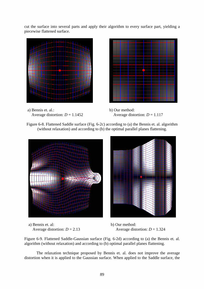
89
cut the surface into several parts and apply their algorithm to every surface part, yielding a piecewise flattened surface.
a) Bennis et. al.: b) Our method: Average distortion: D = 1.1452 Average distortion: D = 1.117
Figure 6-8. Flattened Saddle surface (Fig. 6-2c) according to (a) the Bennis et. al. algorithm (without relaxation) and according to (b) the optimal parallel planes flattening.
a) Bennis et. al: b) Our method: Average distortion: D = 2.13 Average distortion: D = 1.324
Figure 6-9. Flattened Saddle-Gaussian surface (Fig. 6-2d) according to (a) the Bennis et. al. algorithm (without relaxation) and according to (b) optimal parallel planes flattening.
The relaxation technique proposed by Bennis et. al. does not improve the average distortion when it is applied to the Gaussian surface. When applied to the Saddle surface, the
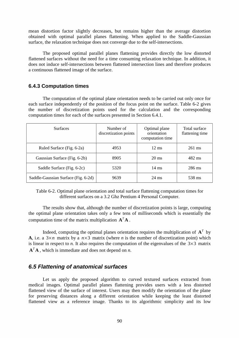
90
mean distortion factor slightly decreases, but remains higher than the average distortion obtained with optimal parallel planes flattening. When applied to the Saddle-Gaussian surface, the relaxation technique does not converge due to the self-intersections.
The proposed optimal parallel planes flattening provides directly the low distorted flattened surfaces without the need for a time consuming relaxation technique. In addition, it does not induce self-intersections between flattened intersection lines and therefore produces a continuous flattened image of the surface.
6.4.3 Computation times
The computation of the optimal plane orientation needs to be carried out only once for each surface independently of the position of the focus point on the surface. Table 6-2 gives the number of discretization points used for the calculation and the corresponding computation times for each of the surfaces presented in Section 6.4.1.
Surfaces Number of discretization points
Optimal plane orientation
computation time
Total surface flattening time
Ruled Surface (Fig. 6-2a) 4953 12 ms 261 ms
Gaussian Surface (Fig. 6-2b) 8905 20 ms 482 ms
Saddle Surface (Fig. 6-2c) 5320 14 ms 286 ms
Saddle-Gaussian Surface (Fig. 6-2d) 9639 24 ms 538 ms
Table 6-2. Optimal plane orientation and total surface flattening computation times for different surfaces on a 3.2 Ghz Pentium 4 Personal Computer.
The results show that, although the number of discretization points is large, computing the optimal plane orientation takes only a few tens of milliseconds which is essentially the computation time of the matrix multiplication TA A .
Indeed, computing the optimal planes orientation requires the multiplication of TA by A, i.e. a 3 n× matrix by a 3n× matrix (where n is the number of discretization point) which is linear in respect to n. It also requires the computation of the eigenvalues of the 3 3× matrix
TA A , which is immediate and does not depend on n.
6.5 Flattening of anatomical surfaces
Let us apply the proposed algorithm to curved textured surfaces extracted from medical images. Optimal parallel planes flattening provides users with a less distorted flattened view of the surface of interest. Users may then modify the orientation of the plane for preserving distances along a different orientation while keeping the least distorted flattened view as a reference image. Thanks to its algorithmic simplicity and its low
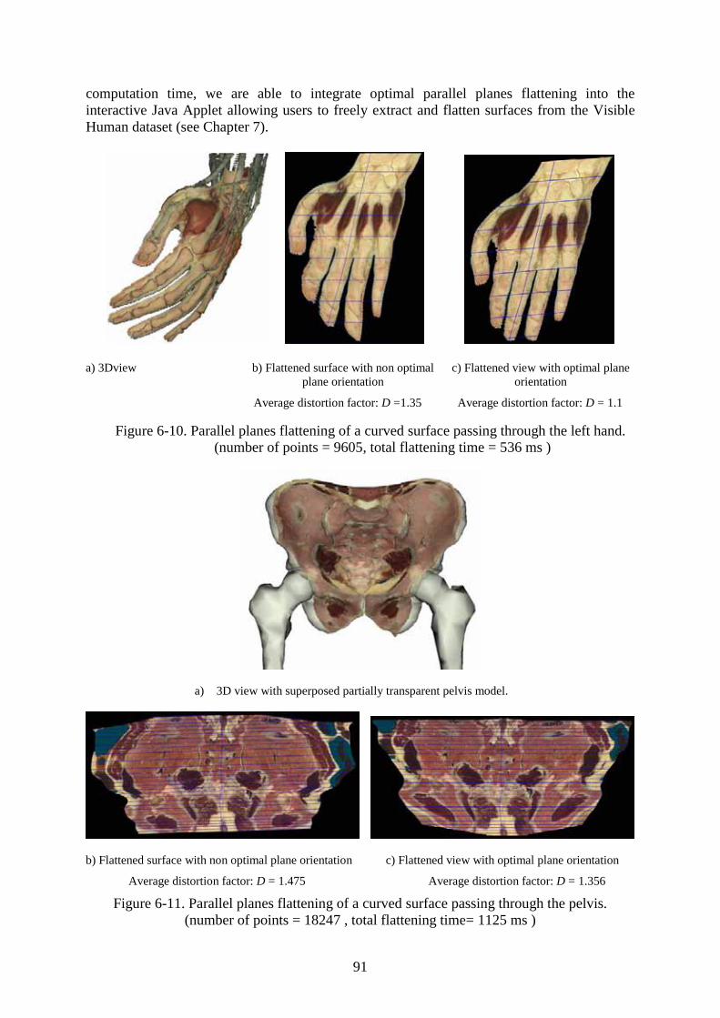
91
computation time, we are able to integrate optimal parallel planes flattening into the interactive Java Applet allowing users to freely extract and flatten surfaces from the Visible Human dataset (see Chapter 7).
a) 3Dview b) Flattened surface with non optimal plane orientation
Average distortion factor: D =1.35
c) Flattened view with optimal plane orientation
Average distortion factor: D = 1.1
Figure 6-10. Parallel planes flattening of a curved surface passing through the left hand. (number of points = 9605, total flattening time = 536 ms )
a) 3D view with superposed partially transparent pelvis model.
b) Flattened surface with non optimal plane orientation c) Flattened view with optimal plane orientation
Average distortion factor: D = 1.475 Average distortion factor: D = 1.356
Figure 6-11. Parallel planes flattening of a curved surface passing through the pelvis. (number of points = 18247 , total flattening time= 1125 ms )
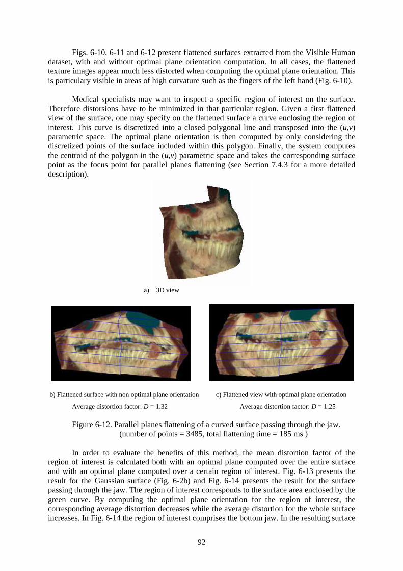
92
Figs. 6-10, 6-11 and 6-12 present flattened surfaces extracted from the Visible Human dataset, with and without optimal plane orientation computation. In all cases, the flattened texture images appear much less distorted when computing the optimal plane orientation. This is particulary visible in areas of high curvature such as the fingers of the left hand (Fig. 6-10).
Medical specialists may want to inspect a specific region of interest on the surface. Therefore distorsions have to be minimized in that particular region. Given a first flattened view of the surface, one may specify on the flattened surface a curve enclosing the region of interest. This curve is discretized into a closed polygonal line and transposed into the (u,v)parametric space. The optimal plane orientation is then computed by only considering the discretized points of the surface included within this polygon. Finally, the system computes the centroid of the polygon in the (u,v) parametric space and takes the corresponding surface point as the focus point for parallel planes flattening (see Section 7.4.3 for a more detailed description).
a) 3D view
b) Flattened surface with non optimal plane orientation c) Flattened view with optimal plane orientation
Average distortion factor: D = 1.32 Average distortion factor: D = 1.25
Figure 6-12. Parallel planes flattening of a curved surface passing through the jaw. (number of points = 3485, total flattening time = 185 ms )
In order to evaluate the benefits of this method, the mean distortion factor of the region of interest is calculated both with an optimal plane computed over the entire surface and with an optimal plane computed over a certain region of interest. Fig. 6-13 presents the result for the Gaussian surface (Fig. 6-2b) and Fig. 6-14 presents the result for the surface passing through the jaw. The region of interest corresponds to the surface area enclosed by the green curve. By computing the optimal plane orientation for the region of interest, the corresponding average distortion decreases while the average distortion for the whole surface increases. In Fig. 6-14 the region of interest comprises the bottom jaw. In the resulting surface
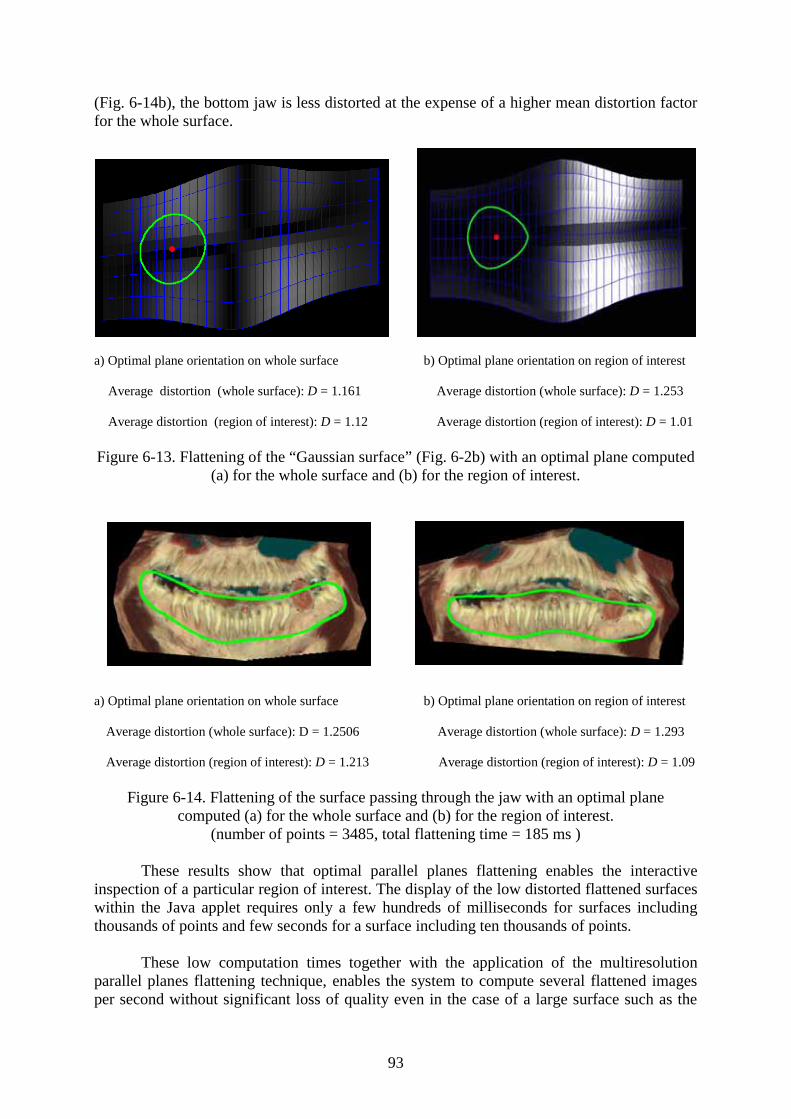
93
(Fig. 6-14b), the bottom jaw is less distorted at the expense of a higher mean distortion factor for the whole surface.
a) Optimal plane orientation on whole surface b) Optimal plane orientation on region of interest
Average distortion (whole surface): D = 1.161 Average distortion (whole surface): D = 1.253
Average distortion (region of interest): D = 1.12 Average distortion (region of interest): D = 1.01
Figure 6-13. Flattening of the “Gaussian surface” (Fig. 6-2b) with an optimal plane computed (a) for the whole surface and (b) for the region of interest.
a) Optimal plane orientation on whole surface b) Optimal plane orientation on region of interest
Average distortion (whole surface): D = 1.2506 Average distortion (whole surface): D = 1.293
Average distortion (region of interest): D = 1.213 Average distortion (region of interest): D = 1.09
Figure 6-14. Flattening of the surface passing through the jaw with an optimal plane computed (a) for the whole surface and (b) for the region of interest.
(number of points = 3485, total flattening time = 185 ms )
These results show that optimal parallel planes flattening enables the interactive inspection of a particular region of interest. The display of the low distorted flattened surfaces within the Java applet requires only a few hundreds of milliseconds for surfaces including thousands of points and few seconds for a surface including ten thousands of points.
These low computation times together with the application of the multiresolution parallel planes flattening technique, enables the system to compute several flattened images per second without significant loss of quality even in the case of a large surface such as the
94
pelvis surface (Fig. 6-11). Multiresolution parallel planes flattening provides a progressive and continuous deformation of the flattened surface according to the displacement of the focus point.
6.6 Conclusion
In this chapter, we have extended parallel planes flattening which preserves distances along one orientation by computing the optimal plane orientation which minimizes the surface flattening distortions. Minimizing the distortions is equivalent to the minimization of the cumulated geodesic curvature along intersection curves between the surface and the parallel planes. Relying on differential geometry, we showed that the reduction of the geodesic curvature at a specific point of the surface is equivalent to the minimization of the scalar product between the plane normal vector and the surface normal at this point. Finding the optimal plane orientation which minimizes in the least square sense this scalar product for the sample points of the considered surface region becomes a principal component analysis problem. The solution is calculated in linear time with respect to the number of sample points.
Unlike most global optimization surface flattening methods, parallel planes surface flattening with optimal surface orientation is therefore fast and seems especially well suited for interactive visualization applications.
Computing an optimal plane orientation yielding intersecting surface curves with theleast cumulated geodesic curvature may be useful in other surface flattening methods [Bennis et. al. 1991], for example in order to create a new set of parametric curves having orientations inducing lower distortions. Curvedness weighting factors may also be useful for improving global optimization methods [Levy and Mallet 1998] when applied to triangulated parametric surfaces, by giving less weight to low curvature surface areas.
95
7 Integration of surface extraction and flattening into the Visible Human server project
In this chapter we present the Visible Human server Java applet which provides users with the means of exploring online the Visible Human dataset by using the curved surface extraction and flattening tools presented in this work. We present the framework of the Visible Human server and the different visualization tools integrated in the Java applet.
7.1 Introduction
EPFL’s Visible Human Web server, created by the Peripheral System Laboratory, offers a number of visualization services to researchers and specialists in anatomy (http://visiblehuman.epfl.ch). These services rely on the Visible Human data sets licensed by the National Library of Medicine [Ackerman 1998] as well as on the Segmented and Classified Visible Human licensed by Gold Standard Multimedia (http://www.gsm.com).
Anatomic structures are often visualized by cross-sections similar to the ones printed in an anatomic atlas. The Visible Human dataset, produced by the National Library of Medicine’s Visible Human Project [Ackerman 1998], provides an excellent resource for generating digital cross-sections. It consists of transverse CT, MRI, and cryosection imagery of a man and a woman. However, working with the full dataset (13 GB for the Visible Man) on a workstation is cumbersome and requires advanced programming skills. By offering access services to the Visible Human data on the Web, a much larger public of students, professionals and researchers can benefit from this instructive anatomical resource.
The first Web application providing users with the possibility to extract slices perpendicular to the main axes was the NPAC Visible Human viewer applet [North et. al. 1996]. The more recent Visible Human Slice and Surface Server [Hersch et. al. 2000] provides access to arbitrarily oriented and positioned slices, as well as to slice sequence animations. These applications require that the user first defines the position and orientation of the slice he wishes to view before getting the resulting cross-section or animation a few seconds later. A first approach for enabling real-time interactive slicing on the web was presented by Gerlach and Hersch [2002]. This Java application allows users to navigate within the Visible Human dataset by continuously extracting slices at a speed of several slices per second. Another applet allows users to construct anatomical 3D scenes comprising slices and anatomical 3D models reconstructed from the labeled dataset [Evesque et. al. 2002]. In this chapter, we present the applet developed within the present thesis, made available to the
96
public on the Visible Human server [Saroul et. al. 2004]. This applet combines real time slice extraction and a 3D anatomical viewer together with the extraction and flattening of curved surfaces. This chapter explains how the surface extraction and flattening tools are integrated into the Java applet and within the Visible Human server.
In Section 7.2, we present the Visible Human server project and describe its framework. In Section 7.3, we explain how slices and surfaces are extracted from the visible Human data located on the server and displayed on the Java applet. Finally, in Section 7.4, we describe the main functionalities of the applet.
7.2 The Visible Human Server project
7.2.1 Previous works
Several related projects aim at making 3D anatomy accessible to students and professionals as well as to a larger public. The Voxel Man system distributed on CD-ROM by Springer Verlag allows users to interact and explore anatomy structures via pre-computed “Intelligent QuickTime Movies” [Schubert et. al. 1999]. The Brain Browser, a system for visualizing the brain, relies on the server side computation of 3D brain structure images and their visualization in the client's applet [Poliakov et. al. 2001]. In the Anatomy Browser, 3D projections along the main orientations as well as axial, coronal and sagittal slices, including labelling information is made available to the client applet [Golland et. al. 1999]. In another project, a VRML interface is used as a tool for visualizing a combination of 3D structures reconstructed from MRI images and planar slices [Warrick and Funnell 1998].
7.2.2 History
The main goal of the EPFL’s Visible Human server project is to offer professionals, researchers and the general public a set of comprehensive services for exploring the Human anatomy. Let us briefly describe the different generations of services developed for the Visible Human server.
Slices, surfaces and animation extraction
First generation services were limited to the extraction of oblique slices [Hersch et. al. 2000], slice animations [Bessaud and Hersch 2000] and ruled surfaces [Figueiredo and Hersch 2002]. Slice extraction was extended to provide support for identifying and highlighting anatomic structures pointed by the user.
Users may specify a slice position and orientation by using a small 3D View of the Visible Human (see Fig. 7-1a). The slice texture is then extracted from the Visible Human dataset and displayed in the Java applet (Fig. 7-1b).
97
a) Slice specification b) Extracted slice
Figure 7-1. First generation services: Slice extraction.
Real-time slice navigation
Figure 7-2. Second generation services: Real-time slice navigation.
Second generation services include a Real-time Navigator [Gerlach and Hersch 2002]. The navigator applet allows users to browse in real-time across the human body by continuously extracting and displaying slices at a speed of several slices per second according to the displacement of the mouse (Fig. 7-2). Thanks to the real-time interaction, one may easily orient slices so as to obtain the most suitable view of a given anatomic structure (Fig. 7-2). For enabling real time navigation on the Web, the application is partitioned between the client (Java Applet) and the Web server.
3D anatomical scene constructor
In order to provide users with more realism, third generation services allow the visualization of the Visible Human within 3D anatomical scenes. The labeled dataset enabled
98
the reconstruction of a high quality collection of 3D anatomical models. The 3D scene viewer applet allows users to construct anatomical scenes, combining 3D organ models and planar slices (see Fig. 7-3). The collection of models resides on the server. By using the server database, a user can load any organ and add it to his scene. Translations, rotations and zooming operations can be applied to virtual scenes. In this project, the client applet provides extensive interaction capabilities for constructing anatomic scenes, is capable of displaying 3D structures in real time, offers both transparent and opaque display modes and allows users to record interactions in order to produce high-quality video sequences. A teacher may create an animation by rotating and zooming and by temporarily discarding certain structures in order to reveal other structures.
Figure 7-3. Third generation services: 3D anatomical structures viewer.
Curved surface extraction and flattening
The last generation services integrate the curved surface extraction and flattening tools presented in this work. The new applet includes a real time navigator and a 3D anatomical structures viewer in order to provide users with a complete set of visualization tools for exploring and studying the Visible Human and for constructing surfaces following curved anatomic structures (see Chapter 3).
7.2.3 Visible Human server framework
Let us now present the Visible Human server framework which is an extension of the one developed by [Evesque et al. 2002]. Due to the large size of the Visible Human dataset (13 GB), it is not possible to transfer it into the client PC. Therefore, a Client-Server framework is used for providing users with access to the data.
The Visible Human dataset is located on a server PC and a communication protocol is used to transfer data to the client application. For instance, the extraction of a slice or a surface is performed on the server PC and the resulting texture image is sent to the client PC for display. Fig. 7-4 shows the framework of the server as well as the distribution of the different tasks between the server and the client.
99
Figure 7-4. Framework of the Visible Human server.
The extraction of a textured surface from the Visible Human dataset is divided into the following tasks:
1. Client PC: Specification of the surface within the Java applet. Computation of a list of control points defining the surface.
2. Client PC: Request for the extraction of textured surface and sending the surface data points to the server PC.
3. Server PC: Reception of the extraction request and reception of the surface data.
4. Server PC: Computation of the surface and extraction of the corresponding surface texture from the Visible Human dataset.
5. Server PC: Replying to the client PC and transmission of the texture data.
6. Client PC: Reception of the texture data.
7. Client PC: Display of the resulting textured surface.
This communication protocol allows users to extract and display textured surfaces from the Visible Human data without having to transfer a large amount of data into the client PC. The server PC also includes a database which contains a list of 3D models which can be loaded within the client Java applet. A 3D model is stored as a file which contains the list of surface triangle vertices. When the user wants to display a 3D model, the client Java applet transfers the corresponding file from the server PC.
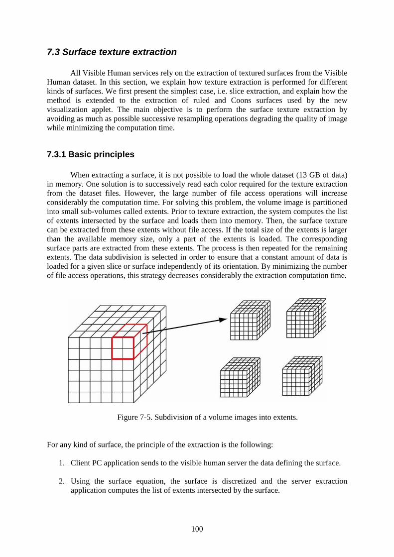
100
7.3 Surface texture extraction
All Visible Human services rely on the extraction of textured surfaces from the Visible Human dataset. In this section, we explain how texture extraction is performed for different kinds of surfaces. We first present the simplest case, i.e. slice extraction, and explain how the method is extended to the extraction of ruled and Coons surfaces used by the new visualization applet. The main objective is to perform the surface texture extraction by avoiding as much as possible successive resampling operations degrading the quality of image while minimizing the computation time.
7.3.1 Basic principles
When extracting a surface, it is not possible to load the whole dataset (13 GB of data) in memory. One solution is to successively read each color required for the texture extraction from the dataset files. However, the large number of file access operations will increase considerably the computation time. For solving this problem, the volume image is partitioned into small sub-volumes called extents. Prior to texture extraction, the system computes the list of extents intersected by the surface and loads them into memory. Then, the surface texture can be extracted from these extents without file access. If the total size of the extents is larger than the available memory size, only a part of the extents is loaded. The corresponding surface parts are extracted from these extents. The process is then repeated for the remaining extents. The data subdivision is selected in order to ensure that a constant amount of data is loaded for a given slice or surface independently of its orientation. By minimizing the number of file access operations, this strategy decreases considerably the extraction computation time.
Figure 7-5. Subdivision of a volume images into extents.
For any kind of surface, the principle of the extraction is the following:
1. Client PC application sends to the visible human server the data defining the surface.
2. Using the surface equation, the surface is discretized and the server extraction application computes the list of extents intersected by the surface.
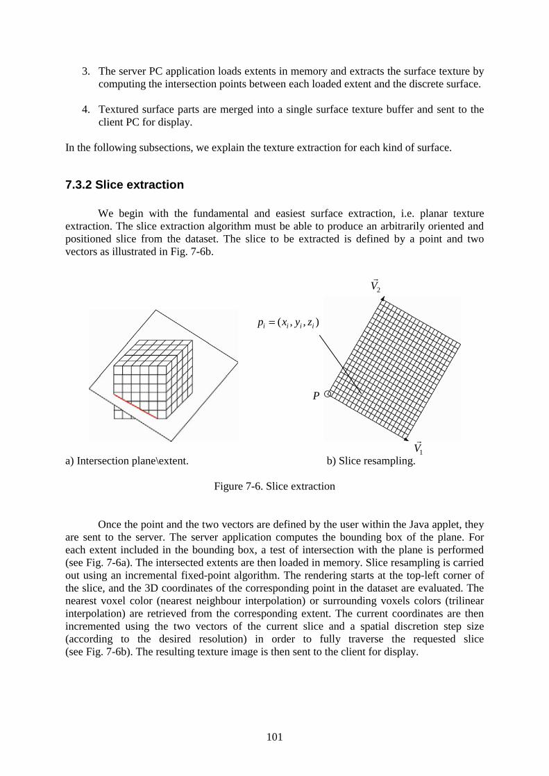
101
3. The server PC application loads extents in memory and extracts the surface texture by computing the intersection points between each loaded extent and the discrete surface.
4. Textured surface parts are merged into a single surface texture buffer and sent to the client PC for display.
In the following subsections, we explain the texture extraction for each kind of surface.
7.3.2 Slice extraction
We begin with the fundamental and easiest surface extraction, i.e. planar texture extraction. The slice extraction algorithm must be able to produce an arbitrarily oriented and positioned slice from the dataset. The slice to be extracted is defined by a point and two vectors as illustrated in Fig. 7-6b.
a) Intersection plane\extent. b) Slice resampling.
Figure 7-6. Slice extraction
Once the point and the two vectors are defined by the user within the Java applet, they are sent to the server. The server application computes the bounding box of the plane. For each extent included in the bounding box, a test of intersection with the plane is performed (see Fig. 7-6a). The intersected extents are then loaded in memory. Slice resampling is carried out using an incremental fixed-point algorithm. The rendering starts at the top-left corner of the slice, and the 3D coordinates of the corresponding point in the dataset are evaluated. The nearest voxel color (nearest neighbour interpolation) or surrounding voxels colors (trilinear interpolation) are retrieved from the corresponding extent. The current coordinates are then incremented using the two vectors of the current slice and a spatial discretion step size (according to the desired resolution) in order to fully traverse the requested slice (see Fig. 7-6b). The resulting texture image is then sent to the client for display.
( , , )i i i ip x y z=
P
2V
1V
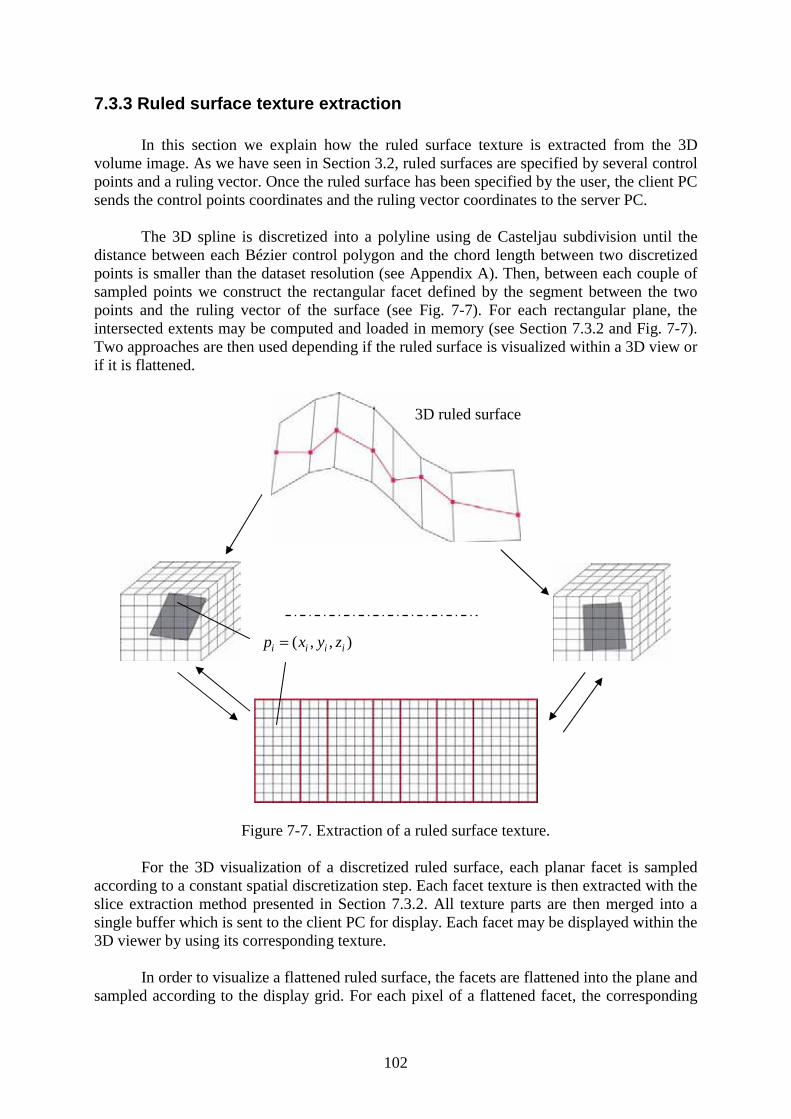
102
7.3.3 Ruled surface texture extraction
In this section we explain how the ruled surface texture is extracted from the 3D volume image. As we have seen in Section 3.2, ruled surfaces are specified by several control points and a ruling vector. Once the ruled surface has been specified by the user, the client PC sends the control points coordinates and the ruling vector coordinates to the server PC.
The 3D spline is discretized into a polyline using de Casteljau subdivision until the distance between each Bézier control polygon and the chord length between two discretized points is smaller than the dataset resolution (see Appendix A). Then, between each couple of sampled points we construct the rectangular facet defined by the segment between the two points and the ruling vector of the surface (see Fig. 7-7). For each rectangular plane, the intersected extents may be computed and loaded in memory (see Section 7.3.2 and Fig. 7-7).Two approaches are then used depending if the ruled surface is visualized within a 3D view or if it is flattened.
Figure 7-7. Extraction of a ruled surface texture.
For the 3D visualization of a discretized ruled surface, each planar facet is sampled according to a constant spatial discretization step. Each facet texture is then extracted with the slice extraction method presented in Section 7.3.2. All texture parts are then merged into a single buffer which is sent to the client PC for display. Each facet may be displayed within the 3D viewer by using its corresponding texture.
In order to visualize a flattened ruled surface, the facets are flattened into the plane and sampled according to the display grid. For each pixel of a flattened facet, the corresponding
3D ruled surface
( , , )i i i ip x y z=
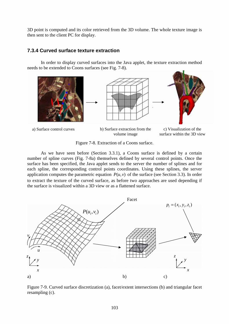
103
3D point is computed and its color retrieved from the 3D volume. The whole texture image is then sent to the client PC for display.
7.3.4 Curved surface texture extraction
In order to display curved surfaces into the Java applet, the texture extraction method needs to be extended to Coons surfaces (see Fig. 7-8).
Figure 7-8. Extraction of a Coons surface.
As we have seen before (Section 3.3.1), a Coons surface is defined by a certain number of spline curves (Fig. 7-8a) themselves defined by several control points. Once the surface has been specified, the Java applet sends to the server the number of splines and for each spline, the corresponding control points coordinates. Using these splines, the server application computes the parametric equation ( , )P u v of the surface (see Section 3.3). In order to extract the texture of the curved surface, as before two approaches are used depending if the surface is visualized within a 3D view or as a flattened surface.
a) b) c)
Figure 7-9. Curved surface discretization (a), facet/extent intersections (b) and triangular facet resampling (c).
a) Surface control curves b) Surface extraction from the volume image
c) Visualization of the surface within the 3D view
( , , )i i i ip x y z=( , )i iP u v
u
v
x
yz
x
yz
Facet
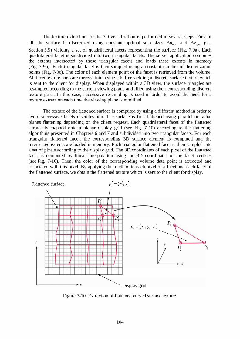
104
The texture extraction for the 3D visualization is performed in several steps. First of all, the surface is discretized using constant optimal step sizes optu∆ and optv∆ (see
Section 5.5) yielding a set of quadrilateral facets representing the surface (Fig. 7.9a). Each quadrilateral facet is subdivided into two triangular facets. The server application computes the extents intersected by these triangular facets and loads these extents in memory (Fig. 7-9b). Each triangular facet is then sampled using a constant number of discretization points (Fig. 7-9c). The color of each element point of the facet is retrieved from the volume. All facet texture parts are merged into a single buffer yielding a discrete surface texture which is sent to the client for display. When displayed within a 3D view, the surface triangles are resampled according to the current viewing plane and filled using their corresponding discrete texture parts. In this case, successive resampling is used in order to avoid the need for a texture extraction each time the viewing plane is modified.
The texture of the flattened surface is computed by using a different method in order to avoid successive facets discretization. The surface is first flattened using parallel or radial planes flattening depending on the client request. Each quadrilateral facet of the flattened surface is mapped onto a planar display grid (see Fig. 7-10) according to the flattening algorithms presented in Chapters 6 and 7 and subdivided into two triangular facets. For each triangular flattened facet, the corresponding 3D surface element is computed and the intersected extents are loaded in memory. Each triangular flattened facet is then sampled into a set of pixels according to the display grid. The 3D coordinates of each pixel of the flattened facet is computed by linear interpolation using the 3D coordinates of the facet vertices (see Fig. 7-10). Then, the color of the corresponding volume data point is extracted and associated with this pixel. By applying this method to each pixel of a facet and each facet of the flattened surface, we obtain the flattened texture which is sent to the client for display.
Figure 7-10. Extraction of flattened curved surface texture.
( , , )i i i ip x y z=
1P′
2P′ 3P′
( , )i i ip x y′ ′ ′=
1P
2P 3P
Flattened surface
Display grid
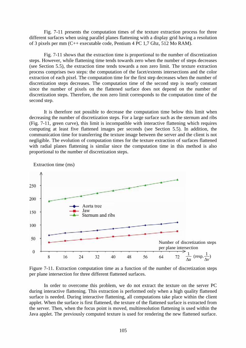
105
Fig. 7-11 presents the computation times of the texture extraction process for three different surfaces when using parallel planes flattening with a display grid having a resolution of 3 pixels per mm (C++ executable code, Pentium 4 PC 1,7 Ghz, 512 Mo RAM).
Fig. 7-11 shows that the extraction time is proportional to the number of discretization steps. However, while flattening time tends towards zero when the number of steps decreases (see Section 5.5), the extraction time tends towards a non zero limit. The texture extraction process comprises two steps: the computation of the facet/extents intersections and the color extraction of each pixel. The computation time for the first step decreases when the number of discretization steps decreases. The computation time of the second step is nearly constant since the number of pixels on the flattened surface does not depend on the number of discretization steps. Therefore, the non zero limit corresponds to the computation time of the second step.
It is therefore not possible to decrease the computation time below this limit when decreasing the number of discretization steps. For a large surface such as the sternum and ribs (Fig. 7-11, green curve), this limit is incompatible with interactive flattening which requires computing at least five flattened images per seconds (see Section 5.5). In addition, the communication time for transferring the texture image between the server and the client is not negligible. The evolution of computation times for the texture extraction of surfaces flattened with radial planes flattening is similar since the computation time in this method is also proportional to the number of discretization steps.
Figure 7-11. Extraction computation time as a function of the number of discretization steps per plane intersection for three different flattened surfaces.
In order to overcome this problem, we do not extract the texture on the server PC during interactive flattening. This extraction is performed only when a high quality flattened surface is needed. During interactive flattening, all computations take place within the client applet. When the surface is first flattened, the texture of the flattened surface is extracted from the server. Then, when the focus point is moved, multiresolution flattening is used within the Java applet. The previously computed texture is used for rendering the new flattened surface.
Extraction time (ms)
Number of discretization steps per plane intersection
1 1 (resp. )u v∆ ∆
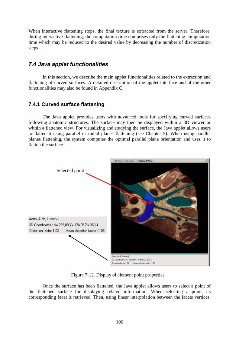
106
When interactive flattening stops, the final texture is extracted from the server. Therefore, during interactive flattening, the computation time comprises only the flattening computation time which may be reduced to the desired value by decreasing the number of discretization steps.
7.4 Java applet functionalities
In this section, we describe the main applet functionalities related to the extraction and flattening of curved surfaces. A detailed description of the applet interface and of the other functionalities may also be found in Appendix C.
7.4.1 Curved surface flattening
The Java applet provides users with advanced tools for specifying curved surfaces following anatomic structures. The surface may then be displayed within a 3D viewer or within a flattened view. For visualizing and studying the surface, the Java applet allows users to flatten it using parallel or radial planes flattening (see Chapter 5). When using parallel planes flattening, the system computes the optimal parallel plane orientation and uses it to flatten the surface.
Figure 7-12. Display of element point properties.
Once the surface has been flattened, the Java applet allows users to select a point of the flattened surface for displaying related information. When selecting a point, its corresponding facet is retrieved. Then, using linear interpolation between the facets vertices,
Selected point
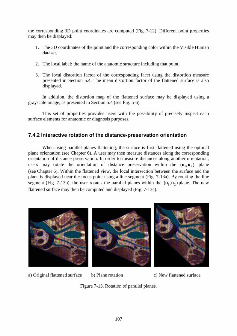
107
the corresponding 3D point coordinates are computed (Fig. 7-12). Different point properties may then be displayed:
1. The 3D coordinates of the point and the corresponding color within the Visible Human dataset.
2. The local label: the name of the anatomic structure including that point.
3. The local distortion factor of the corresponding facet using the distortion measure presented in Section 5.4. The mean distortion factor of the flattened surface is also displayed.
In addition, the distortion map of the flattened surface may be displayed using a grayscale image, as presented in Section 5.4 (see Fig. 5-6).
This set of properties provides users with the possibility of precisely inspect each surface elements for anatomic or diagnosis purposes.
7.4.2 Interactive rotation of the distance-preservation orientation
When using parallel planes flattening, the surface is first flattened using the optimal plane orientation (see Chapter 6). A user may then measure distances along the corresponding orientation of distance preservation. In order to measure distances along another orientation, users may rotate the orientation of distance preservation within the 1 2( , )u u plane
(see Chapter 6). Within the flattened view, the local intersection between the surface and the plane is displayed near the focus point using a line segment (Fig. 7-13a). By rotating the line segment (Fig. 7-13b), the user rotates the parallel planes within the 1 2( , )u u plane. The new
flattened surface may then be computed and displayed (Fig. 7-13c).
a) Original flattened surface b) Plane rotation c) New flattened surface
Figure 7-13. Rotation of parallel planes.
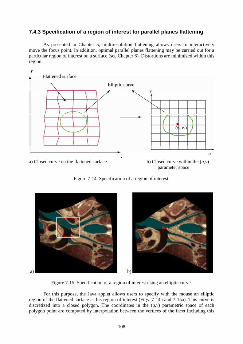
108
7.4.3 Specification of a region of interest for parallel planes flattening
As presented in Chapter 5, multiresolution flattening allows users to interactively move the focus point. In addition, optimal parallel planes flattening may be carried out for a particular region of interest on a surface (see Chapter 6). Distortions are minimized within this region.
a) Closed curve on the flattened surface b) Closed curve within the (u,v)parameter space
Figure 7-14. Specification of a region of interest.
a) b)
Figure 7-15. Specification of a region of interest using an elliptic curve.
For this purpose, the Java applet allows users to specify with the mouse an elliptic region of the flattened surface as his region of interest (Figs. 7-14a and 7-15a). This curve is discretized into a closed polygon. The coordinates in the (u,v) parametric space of each polygon point are computed by interpolation between the vertices of the facet including this
u
v
0 0( , )u v
x
y
Elliptic curve
Flattened surface
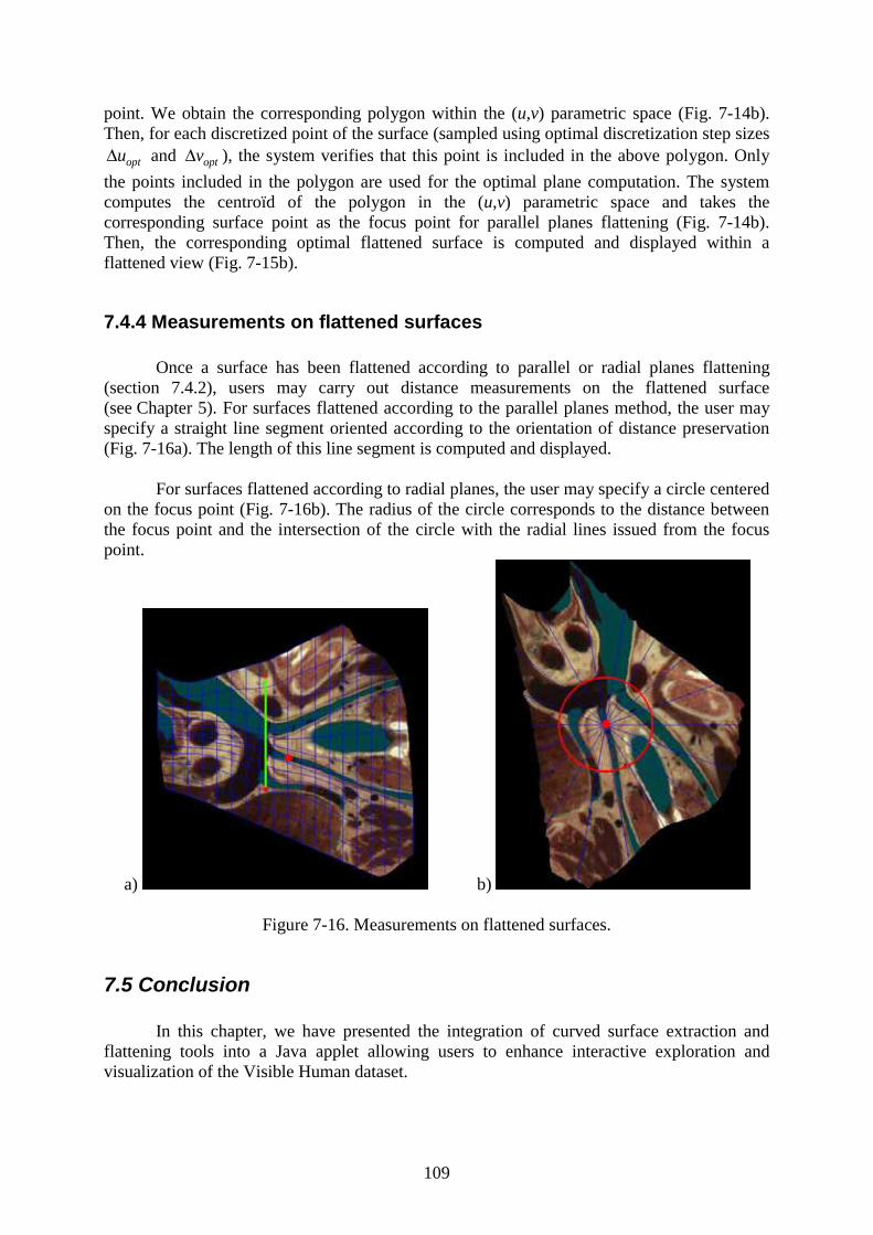
109
point. We obtain the corresponding polygon within the (u,v) parametric space (Fig. 7-14b). Then, for each discretized point of the surface (sampled using optimal discretization step sizes
optu∆ and optv∆ ), the system verifies that this point is included in the above polygon. Only
the points included in the polygon are used for the optimal plane computation. The system computes the centroïd of the polygon in the (u,v) parametric space and takes the corresponding surface point as the focus point for parallel planes flattening (Fig. 7-14b). Then, the corresponding optimal flattened surface is computed and displayed within a flattened view (Fig. 7-15b).
7.4.4 Measurements on flattened surfaces
Once a surface has been flattened according to parallel or radial planes flattening (section 7.4.2), users may carry out distance measurements on the flattened surface (see Chapter 5). For surfaces flattened according to the parallel planes method, the user may specify a straight line segment oriented according to the orientation of distance preservation (Fig. 7-16a). The length of this line segment is computed and displayed.
For surfaces flattened according to radial planes, the user may specify a circle centered on the focus point (Fig. 7-16b). The radius of the circle corresponds to the distance between the focus point and the intersection of the circle with the radial lines issued from the focus point.
a) b)
Figure 7-16. Measurements on flattened surfaces.
7.5 Conclusion
In this chapter, we have presented the integration of curved surface extraction and flattening tools into a Java applet allowing users to enhance interactive exploration and visualization of the Visible Human dataset.

110
In order to provide users with an online access to the Visible Human, the extraction and flattening tools are distributed between the Java applet and the Visible Human server. The specification and display of curved surfaces take place within the Java applet, while the texture extraction is performed on the Visible Human server. A communication protocol allows the Java applet to request surface texture extraction and to receive the resulting texture image from the server.
Moreover, this applet allows the users to precisely visualize and study surface properties. For each point of the flattened surface, its 3D coordinates, color, label and distortion factor may be displayed. In addition to interactive flattening, users may select a region of interest where distortions are to be minimized. Tools for measuring distances along curved surface is provided thanks to the distance preserving flattening methods presented in Chapter 6. The Java applet therefore provides a means of precisely and interactively inspecting the Visible Human data.
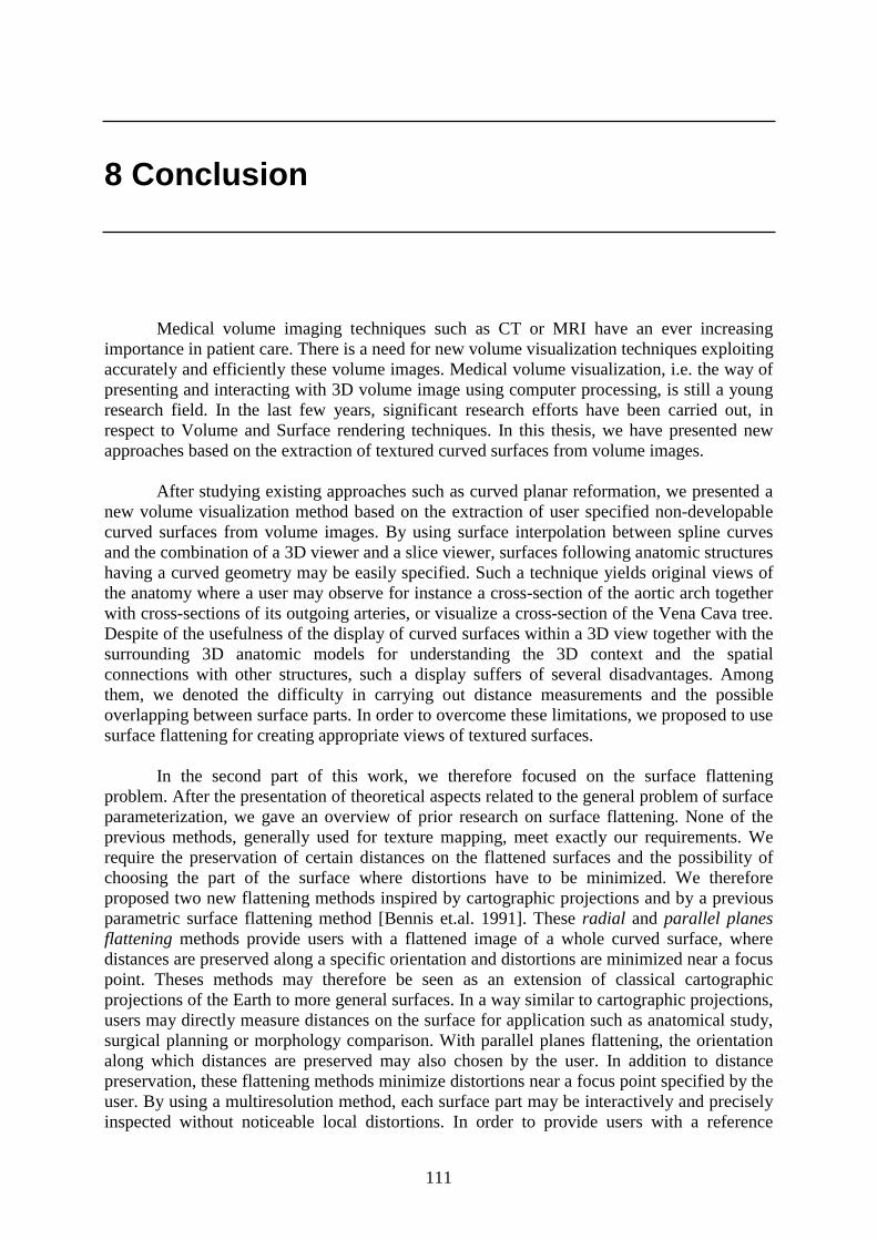
111
8 Conclusion
Medical volume imaging techniques such as CT or MRI have an ever increasing importance in patient care. There is a need for new volume visualization techniques exploiting accurately and efficiently these volume images. Medical volume visualization, i.e. the way of presenting and interacting with 3D volume image using computer processing, is still a young research field. In the last few years, significant research efforts have been carried out, in respect to Volume and Surface rendering techniques. In this thesis, we have presented new approaches based on the extraction of textured curved surfaces from volume images.
After studying existing approaches such as curved planar reformation, we presented a new volume visualization method based on the extraction of user specified non-developable curved surfaces from volume images. By using surface interpolation between spline curves and the combination of a 3D viewer and a slice viewer, surfaces following anatomic structures having a curved geometry may be easily specified. Such a technique yields original views of the anatomy where a user may observe for instance a cross-section of the aortic arch together with cross-sections of its outgoing arteries, or visualize a cross-section of the Vena Cava tree. Despite of the usefulness of the display of curved surfaces within a 3D view together with the surrounding 3D anatomic models for understanding the 3D context and the spatial connections with other structures, such a display suffers of several disadvantages. Among them, we denoted the difficulty in carrying out distance measurements and the possible overlapping between surface parts. In order to overcome these limitations, we proposed to use surface flattening for creating appropriate views of textured surfaces.
In the second part of this work, we therefore focused on the surface flattening problem. After the presentation of theoretical aspects related to the general problem of surface parameterization, we gave an overview of prior research on surface flattening. None of the previous methods, generally used for texture mapping, meet exactly our requirements. We require the preservation of certain distances on the flattened surfaces and the possibility of choosing the part of the surface where distortions have to be minimized. We therefore proposed two new flattening methods inspired by cartographic projections and by a previous parametric surface flattening method [Bennis et.al. 1991]. These radial and parallel planes flattening methods provide users with a flattened image of a whole curved surface, where distances are preserved along a specific orientation and distortions are minimized near a focus point. Theses methods may therefore be seen as an extension of classical cartographic projections of the Earth to more general surfaces. In a way similar to cartographic projections, users may directly measure distances on the surface for application such as anatomical study, surgical planning or morphology comparison. With parallel planes flattening, the orientation along which distances are preserved may also chosen by the user. In addition to distance preservation, these flattening methods minimize distortions near a focus point specified by the user. By using a multiresolution method, each surface part may be interactively and precisely inspected without noticeable local distortions. In order to provide users with a reference
112
flattened image of the surface, parallel planes flattening was extended by computing the parallel planes orientation minimizing the global distortions. The method is based on the minimization of geodesic curvature via a principal component analysis. It yields low surface distortions at a very low computation effort. Such a method seems therefore appropriate for interactive flattening applications, where computation time is limited.
Finally, we presented the integration of the curved surface extraction and flattening tools into the Visible Human server project. These tools are fully integrated into a Java client-server web application providing users with access to the Visible Human. This application also integrates several functionalities allowing users to explore the Visible Human volume image and to test the visualization tools presented in this work.
Our attempt to provide users with new visualization tools for exploring volume images was very successful. We have demonstrated that it is possible to easily specify and extract surfaces following highly curved anatomic structures. We have also shown the usefulness of such curved surface extraction for revealing the connections between anatomic structures and, more generally, for providing users with new interesting views of the anatomy. In addition, surface flattening allows users to precisely inspect curved surfaces, to carry out distance measurements, and to illustrate properties of curved anatomic structures. Such flattened images also provide students with new interesting views for learning anatomy which may complement the traditional anatomical atlases. By using the interactive Java visualization applet, teachers of anatomy may create their own flattened surfaces and may use them for illustrating anatomical lessons.
From a theoretical and technical point of view, we created a new simple and efficient flattening method providing excellent results in terms of distortion minimization. The method of geodesic curvature minimization used in this algorithm also represents an original theoretical contribution to computer graphics. We have also shown that curved surface extraction and flattening may be carried out interactively despite of the large size of the volume image by using a client-server architecture and time efficient algorithms.
The research on extraction and flattening of curved surfaces started with this thesis may be pursued in several directions. For instance, the method of geodesic curvature minimization developed for the parallel planes flattening may be used in texture mapping or other computer graphics applications requiring the computation of surface curves having a minimal cumulated geodesic curvature. Another research track is the medical application of these tools, which needs to be experimented in collaboration with medical specialists, for instance for medical diagnosis or surgical planning purposes. Another possible application is the use of curved surface extraction and flattening for carrying out geometric morphometric measurements, i.e. the measurements of biological shapes in anatomic morphology studies [Richtsmeier et. al. 2002]. The distance preserving flattening methods may provide specialists with a way of carrying out distance measurements between landmarks located on curved surfaces for the study and the characterisation of the geometric properties of curved anatomic structures.
Most medical visualization applications integrate many visualization approaches. Curved surface extraction may become one visualization component. Surface rendering and volume rendering provide users with an understanding of the 3D context while curved surface extraction may be used in complement to enhance or validate diagnosis. For instance, once a tumor has been depicted using surface or volume rendering, medical specialists may extract

113
curved surfaces to track the curved geometry of the corresponding anatomic structure, in order to reveal the mass of the tumor and its involvement in surrounding organs.

114
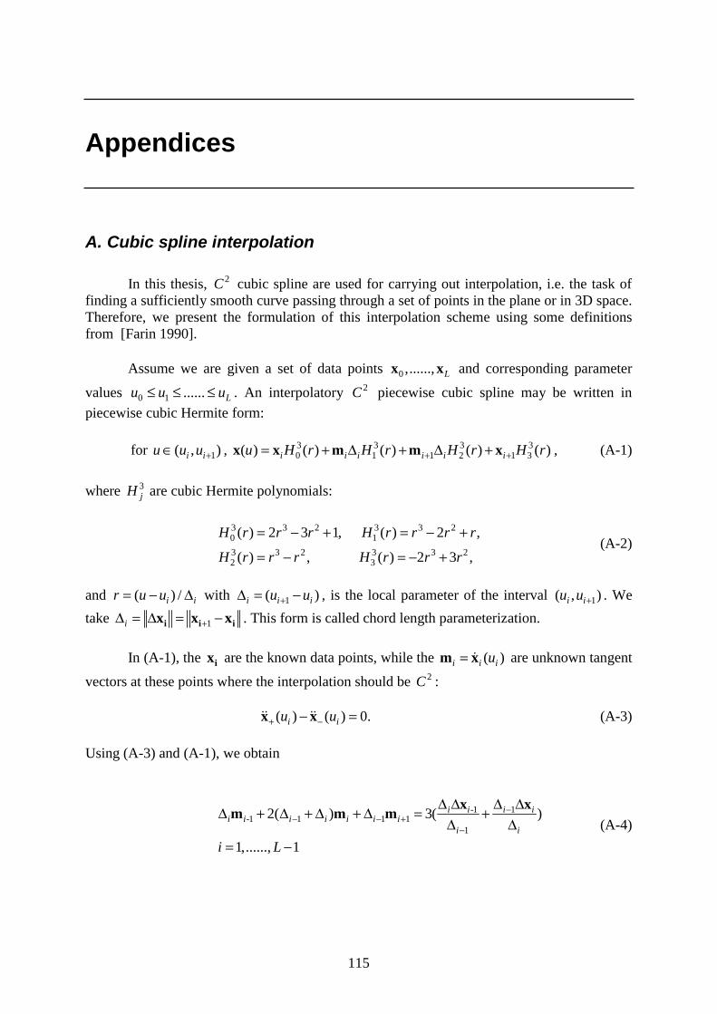
115
Appendices
A. Cubic spline interpolation
In this thesis, 2C cubic spline are used for carrying out interpolation, i.e. the task of finding a sufficiently smooth curve passing through a set of points in the plane or in 3D space. Therefore, we present the formulation of this interpolation scheme using some definitions from [Farin 1990].
Assume we are given a set of data points 0 ,......, Lx x and corresponding parameter
values 0 1 ...... Lu u u≤ ≤ ≤ . An interpolatory 2C piecewise cubic spline may be written in
piecewise cubic Hermite form:
for 1( , )i iu u u +∈ , 3 3 3 30 1 1 2 1 3( ) ( ) ( ) ( ) ( )i i i i i iu H r H r H r H r+ += + ∆ + ∆ +x x m m x , (A-1)
where 3jH are cubic Hermite polynomials:
3 3 2 3 3 20 1
3 3 2 3 3 22 3
( ) 2 3 1, ( ) 2 ,
( ) , ( ) 2 3 ,
H r r r H r r r r
H r r r H r r r
= − + = − +
= − = − + (A-2)
and ( ) /i ir u u= − ∆ with 1( )i i iu u+∆ = − , is the local parameter of the interval 1( , )i iu u + . We
take 1i +∆ = ∆ = −i i ix x x . This form is called chord length parameterization.
In (A-1), the ix are the known data points, while the ( )i i iu=m x are unknown tangent
vectors at these points where the interpolation should be 2C :
( ) ( ) 0.i iu u+ −− =x x (A-3)
Using (A-3) and (A-1), we obtain
-1 1-1 1 1 1
1
2( ) 3( )
1,......, 1
i i i ii i i i i i i
i i
i L
−− − +
−
∆ ∆ ∆ ∆∆ + ∆ + ∆ + ∆ = +∆ ∆
= −
x xm m m
(A-4)
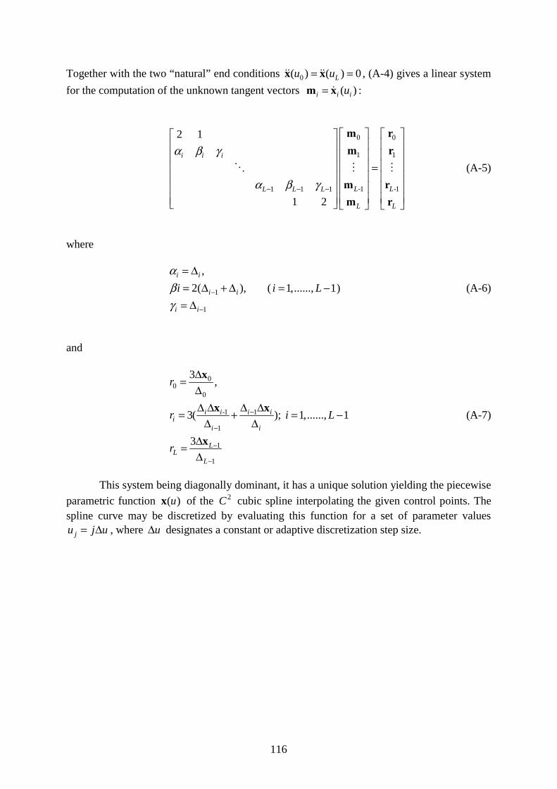
116
Together with the two “natural” end conditions 0( ) ( ) 0Lu u= =x x , (A-4) gives a linear system
for the computation of the unknown tangent vectors ( )i i iu=m x :
0 0
1 1
-1 -11 1 1
2 1
1 2
i i i
L LL L L
L L
α β γ
α β γ− − −
=
m r
m r
m r
m r
(A-5)
where
1
1
,
2( ),i i
i i
i i
i
αβγ
−
−
= ∆= ∆ + ∆= ∆
( 1,......, 1i L= − ) (A-6)
and
00
0
-1 1
1
1
1
3,
3( ); 1,......, 1
3
i i i ii
i i
LL
L
r
r i L
r
−
−
−
−
∆=∆∆ ∆ ∆ ∆= + = −
∆ ∆∆=∆
x
x x
x
(A-7)
This system being diagonally dominant, it has a unique solution yielding the piecewise
parametric function ( )ux of the 2C cubic spline interpolating the given control points. The spline curve may be discretized by evaluating this function for a set of parameter values
ju j u= ∆ , where u∆ designates a constant or adaptive discretization step size.
117
B. Glossary of medical terms
Aorta: The largest artery in the body, the aorta arises from the left ventricle of the heart (see Fig. B-1), slightly ascends, bends over, and then descends through the chest and the abdomen. Then, it is divided into two arteries called the common iliac arteries that go to the legs. Anatomists traditionally divide the aorta into three parts: the ascending aorta, the aortic arch, and the descending aorta.
Aortic arch: The second section of the aorta (see Fig. B-1). The aorta first ascends, then bends, and then descends. The bending part is the aortic arch. The brachiocephalic trunk, the left common carotid artery, and the left subclavian artery start from the aortic arch. In this thesis, the aortic arch with the three outgoing arteries is sometimes called aorta tree.
Atrium Cavity: One of the upper chambers of the heart taking blood from the veins and pumping it into a ventricle. In this thesis, the Atrium Cavity designates the right atrium of the heart at the junction between the Vena Cava superior and the Vena Cava inferior (see Fig. B-1).
Costal cartilages: Bars of hyaline cartilage which serve to prolong the ribs forward and contribute to the elasticity of the walls of the thorax (see Fig. B-2). The first seven pairs are connected with the sternum; the next three are articulated with the lower border of the cartilage of the preceding rib; the last two have sharp extremities ending in the wall of the abdomen.
Cryosection: A medical imaging technique which uses photographic digital images of a frozen body. The body is cut into many slices which are digitally photographed for constituting a 3D volume image of the body.
CT or Computed Tomography: The main medical imaging method where a thin X-ray beam rotates around the patient. Detectors measure the amount of X-rays passing through the patient or particular area of interest. Geometric processing is then used to reconstruct axial two-dimensional X-ray image. The series of axial images enable the reconstruction of a 3D volume image. The word "tomography" is derived from the Greek tomos (slice) and graphia (describing).
MRI or Magnetic Resonance Imaging: A medical imaging technique in which a strong magnetic field controlled by computer is used for modifying the spin of protons of water molecules. The spin relaxation is then analized for generating detailed pictures of areas inside the body. MRI makes better images of organs and soft tissue than other scanning techniques, such as X-ray CT. MRI is especially useful for imaging the brain, spine, the soft tissue of joints, and the inside of bones.
Pelvis: A basin-shaped structure of the vertebrate skeleton, composed of the innominate bones on the sides, the pubis in front, and the sacrum and coccyx behind, that rests on the lower limbs and supports the spinal column (see Fig. B-3).
PET or Positron Emission Tomography: A medical imaging technique based on the fixation of short-lived radioactive substances on active sites such as tumoural sites to produce
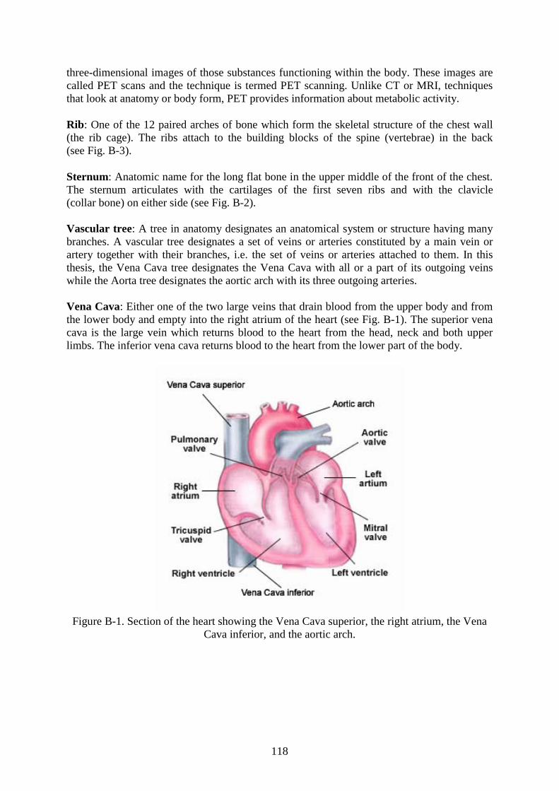
118
three-dimensional images of those substances functioning within the body. These images are called PET scans and the technique is termed PET scanning. Unlike CT or MRI, techniques that look at anatomy or body form, PET provides information about metabolic activity.
Rib: One of the 12 paired arches of bone which form the skeletal structure of the chest wall (the rib cage). The ribs attach to the building blocks of the spine (vertebrae) in the back (see Fig. B-3).
Sternum: Anatomic name for the long flat bone in the upper middle of the front of the chest. The sternum articulates with the cartilages of the first seven ribs and with the clavicle (collar bone) on either side (see Fig. B-2).
Vascular tree: A tree in anatomy designates an anatomical system or structure having many branches. A vascular tree designates a set of veins or arteries constituted by a main vein or artery together with their branches, i.e. the set of veins or arteries attached to them. In this thesis, the Vena Cava tree designates the Vena Cava with all or a part of its outgoing veins while the Aorta tree designates the aortic arch with its three outgoing arteries.
Vena Cava: Either one of the two large veins that drain blood from the upper body and from the lower body and empty into the right atrium of the heart (see Fig. B-1). The superior vena cava is the large vein which returns blood to the heart from the head, neck and both upper limbs. The inferior vena cava returns blood to the heart from the lower part of the body.
Figure B-1. Section of the heart showing the Vena Cava superior, the right atrium, the Vena Cava inferior, and the aortic arch.
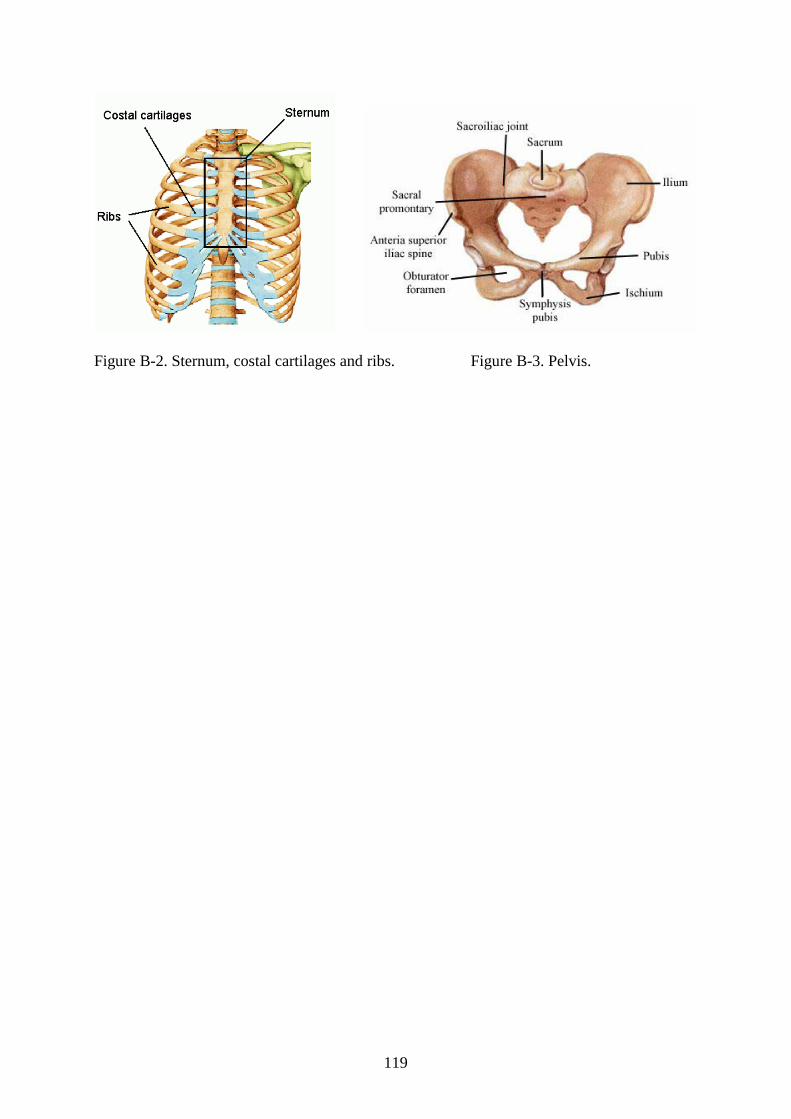
119
Figure B-2. Sternum, costal cartilages and ribs. Figure B-3. Pelvis.
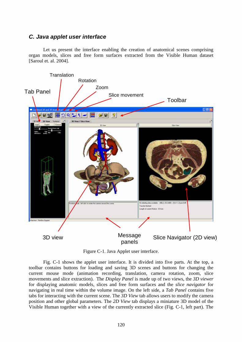
120
C. Java applet user interface
Let us present the interface enabling the creation of anatomical scenes comprising organ models, slices and free form surfaces extracted from the Visible Human dataset [Saroul et. al. 2004].
Figure C-1. Java Applet user interface.
Fig. C-1 shows the applet user interface. It is divided into five parts. At the top, a toolbar contains buttons for loading and saving 3D scenes and buttons for changing the current mouse mode (animation recording, translation, camera rotation, zoom, slice movements and slice extraction). The Display Panel is made up of two views, the 3D viewerfor displaying anatomic models, slices and free form surfaces and the slice navigator for navigating in real time within the volume image. On the left side, a Tab Panel contains five tabs for interacting with the current scene. The 3D View tab allows users to modify the camera position and other global parameters. The 2D View tab displays a miniature 3D model of the Visible Human together with a view of the currently extracted slice (Fig. C-1, left part). The
Tab Panel
Toolbar
3D view Slice Navigator (2D view) Message panels
Slice movement
ZoomRotation
Translation
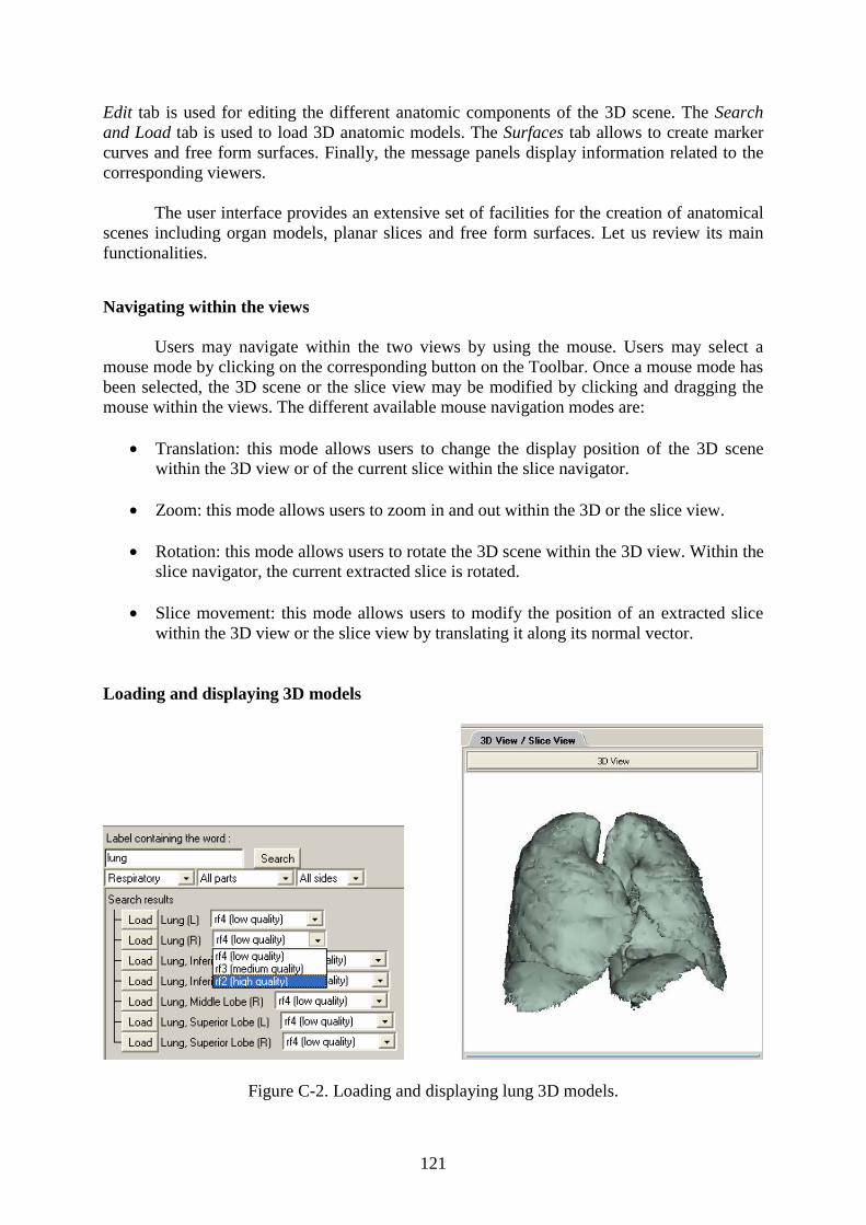
121
Edit tab is used for editing the different anatomic components of the 3D scene. The Search and Load tab is used to load 3D anatomic models. The Surfaces tab allows to create marker curves and free form surfaces. Finally, the message panels display information related to the corresponding viewers.
The user interface provides an extensive set of facilities for the creation of anatomical scenes including organ models, planar slices and free form surfaces. Let us review its main functionalities.
Navigating within the views
Users may navigate within the two views by using the mouse. Users may select a mouse mode by clicking on the corresponding button on the Toolbar. Once a mouse mode has been selected, the 3D scene or the slice view may be modified by clicking and dragging the mouse within the views. The different available mouse navigation modes are:
• Translation: this mode allows users to change the display position of the 3D scene within the 3D view or of the current slice within the slice navigator.
• Zoom: this mode allows users to zoom in and out within the 3D or the slice view.
• Rotation: this mode allows users to rotate the 3D scene within the 3D view. Within the slice navigator, the current extracted slice is rotated.
• Slice movement: this mode allows users to modify the position of an extracted slice within the 3D view or the slice view by translating it along its normal vector.
Loading and displaying 3D models
Figure C-2. Loading and displaying lung 3D models.
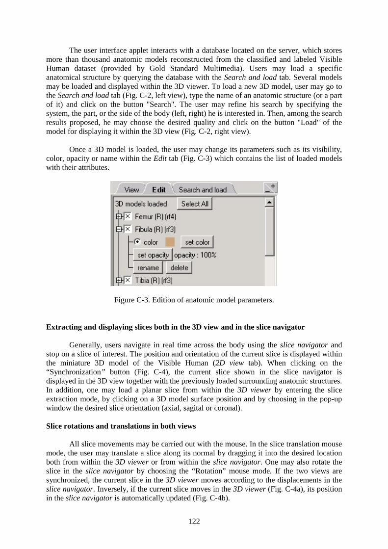
122
The user interface applet interacts with a database located on the server, which stores more than thousand anatomic models reconstructed from the classified and labeled Visible Human dataset (provided by Gold Standard Multimedia). Users may load a specific anatomical structure by querying the database with the Search and load tab. Several models may be loaded and displayed within the 3D viewer. To load a new 3D model, user may go to the Search and load tab (Fig. C-2, left view), type the name of an anatomic structure (or a part of it) and click on the button "Search". The user may refine his search by specifying the system, the part, or the side of the body (left, right) he is interested in. Then, among the search results proposed, he may choose the desired quality and click on the button "Load" of the model for displaying it within the 3D view (Fig. C-2, right view).
Once a 3D model is loaded, the user may change its parameters such as its visibility, color, opacity or name within the Edit tab (Fig. C-3) which contains the list of loaded models with their attributes.
Figure C-3. Edition of anatomic model parameters.
Extracting and displaying slices both in the 3D view and in the slice navigator
Generally, users navigate in real time across the body using the slice navigator and stop on a slice of interest. The position and orientation of the current slice is displayed within the miniature 3D model of the Visible Human (2D view tab). When clicking on the “Synchronization” button (Fig. C-4), the current slice shown in the slice navigator is displayed in the 3D view together with the previously loaded surrounding anatomic structures. In addition, one may load a planar slice from within the 3D viewer by entering the slice extraction mode, by clicking on a 3D model surface position and by choosing in the pop-up window the desired slice orientation (axial, sagital or coronal).
Slice rotations and translations in both views
All slice movements may be carried out with the mouse. In the slice translation mouse mode, the user may translate a slice along its normal by dragging it into the desired location both from within the 3D viewer or from within the slice navigator. One may also rotate the slice in the slice navigator by choosing the “Rotation” mouse mode. If the two views are synchronized, the current slice in the 3D viewer moves according to the displacements in the slice navigator. Inversely, if the current slice moves in the 3D viewer (Fig. C-4a), its position in the slice navigator is automatically updated (Fig. C-4b).
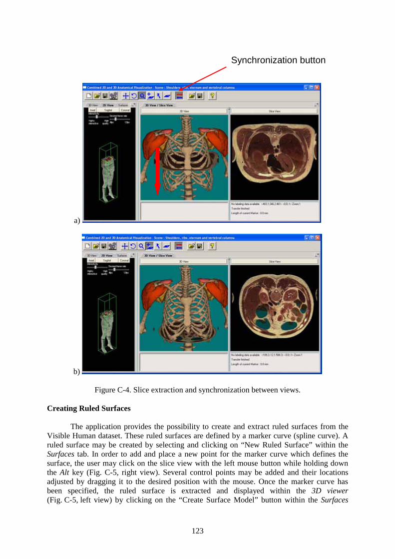
123
a)
b)
Figure C-4. Slice extraction and synchronization between views.
Creating Ruled Surfaces
The application provides the possibility to create and extract ruled surfaces from the Visible Human dataset. These ruled surfaces are defined by a marker curve (spline curve). A ruled surface may be created by selecting and clicking on “New Ruled Surface” within the Surfaces tab. In order to add and place a new point for the marker curve which defines the surface, the user may click on the slice view with the left mouse button while holding down the Alt key (Fig. C-5, right view). Several control points may be added and their locations adjusted by dragging it to the desired position with the mouse. Once the marker curve has been specified, the ruled surface is extracted and displayed within the 3D viewer(Fig. C-5, left view) by clicking on the “Create Surface Model” button within the Surfaces
Synchronization button
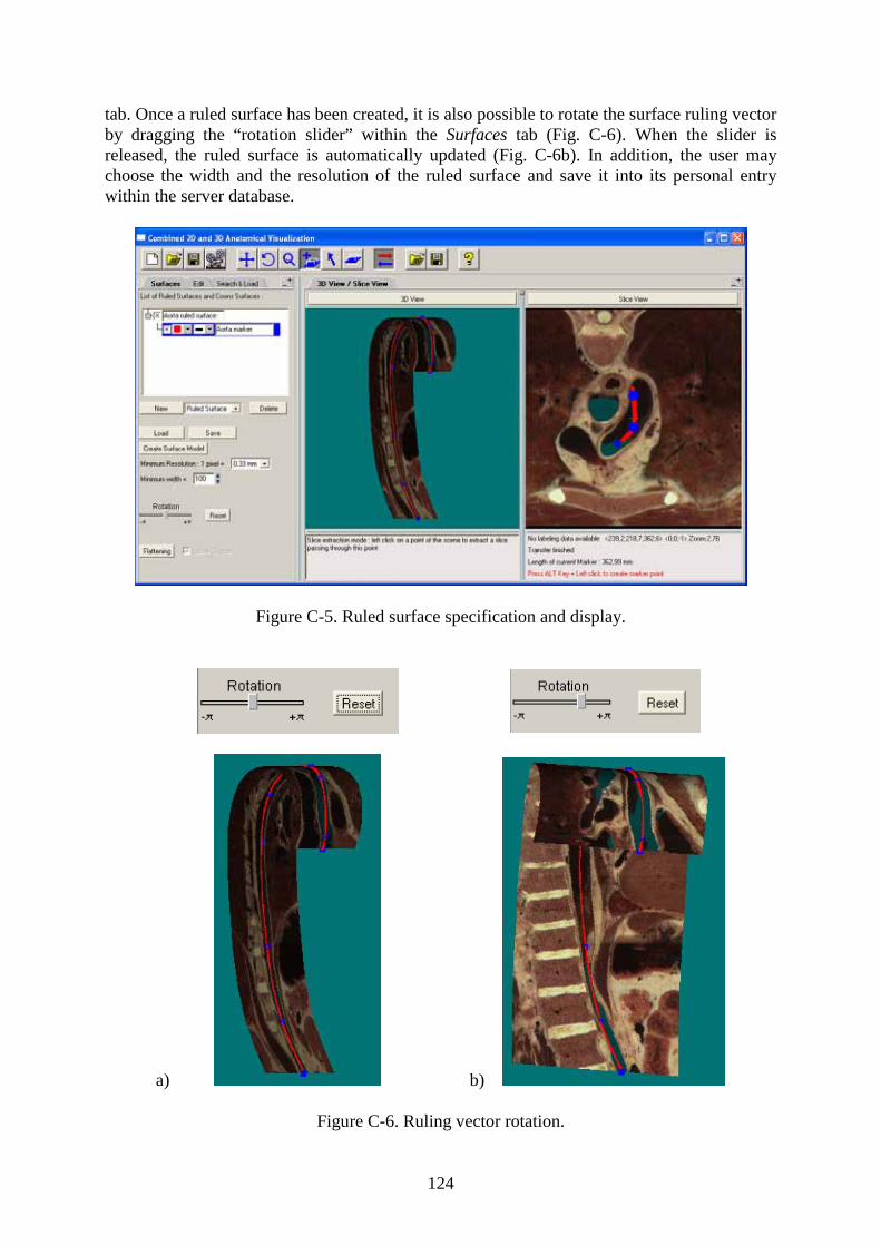
124
tab. Once a ruled surface has been created, it is also possible to rotate the surface ruling vector by dragging the “rotation slider” within the Surfaces tab (Fig. C-6). When the slider is released, the ruled surface is automatically updated (Fig. C-6b). In addition, the user may choose the width and the resolution of the ruled surface and save it into its personal entry within the server database.
Figure C-5. Ruled surface specification and display.
a) b)
Figure C-6. Ruling vector rotation.
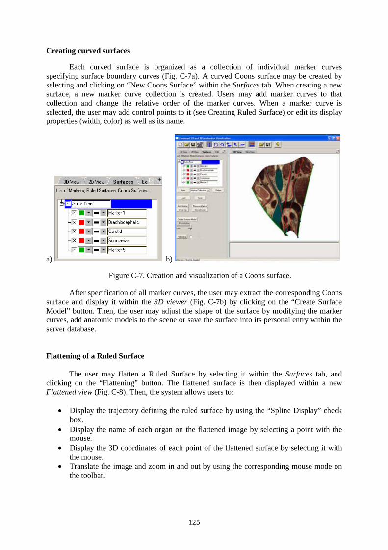
125
Creating curved surfaces
Each curved surface is organized as a collection of individual marker curves specifying surface boundary curves (Fig. C-7a). A curved Coons surface may be created by selecting and clicking on “New Coons Surface” within the Surfaces tab. When creating a new surface, a new marker curve collection is created. Users may add marker curves to that collection and change the relative order of the marker curves. When a marker curve is selected, the user may add control points to it (see Creating Ruled Surface) or edit its display properties (width, color) as well as its name.
a) b)
Figure C-7. Creation and visualization of a Coons surface.
After specification of all marker curves, the user may extract the corresponding Coons surface and display it within the 3D viewer (Fig. C-7b) by clicking on the “Create Surface Model” button. Then, the user may adjust the shape of the surface by modifying the marker curves, add anatomic models to the scene or save the surface into its personal entry within the server database.
Flattening of a Ruled Surface
The user may flatten a Ruled Surface by selecting it within the Surfaces tab, and clicking on the “Flattening” button. The flattened surface is then displayed within a new Flattened view (Fig. C-8). Then, the system allows users to:
• Display the trajectory defining the ruled surface by using the “Spline Display” check box.
• Display the name of each organ on the flattened image by selecting a point with the mouse.
• Display the 3D coordinates of each point of the flattened surface by selecting it with the mouse.
• Translate the image and zoom in and out by using the corresponding mouse mode on the toolbar.
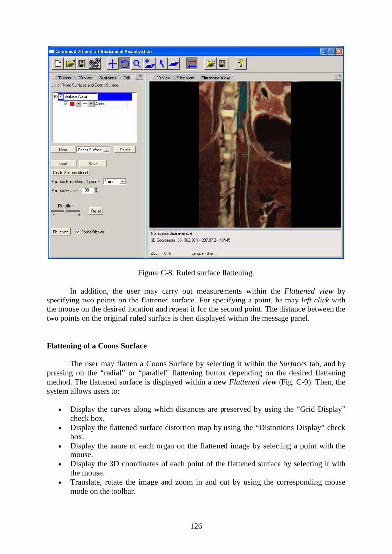
126
Figure C-8. Ruled surface flattening.
In addition, the user may carry out measurements within the Flattened view by specifying two points on the flattened surface. For specifying a point, he may left click with the mouse on the desired location and repeat it for the second point. The distance between the two points on the original ruled surface is then displayed within the message panel.
Flattening of a Coons Surface
The user may flatten a Coons Surface by selecting it within the Surfaces tab, and by pressing on the “radial” or “parallel” flattening button depending on the desired flattening method. The flattened surface is displayed within a new Flattened view (Fig. C-9). Then, the system allows users to:
• Display the curves along which distances are preserved by using the “Grid Display” check box.
• Display the flattened surface distortion map by using the “Distortions Display” check box.
• Display the name of each organ on the flattened image by selecting a point with the mouse.
• Display the 3D coordinates of each point of the flattened surface by selecting it with the mouse.
• Translate, rotate the image and zoom in and out by using the corresponding mouse mode on the toolbar.
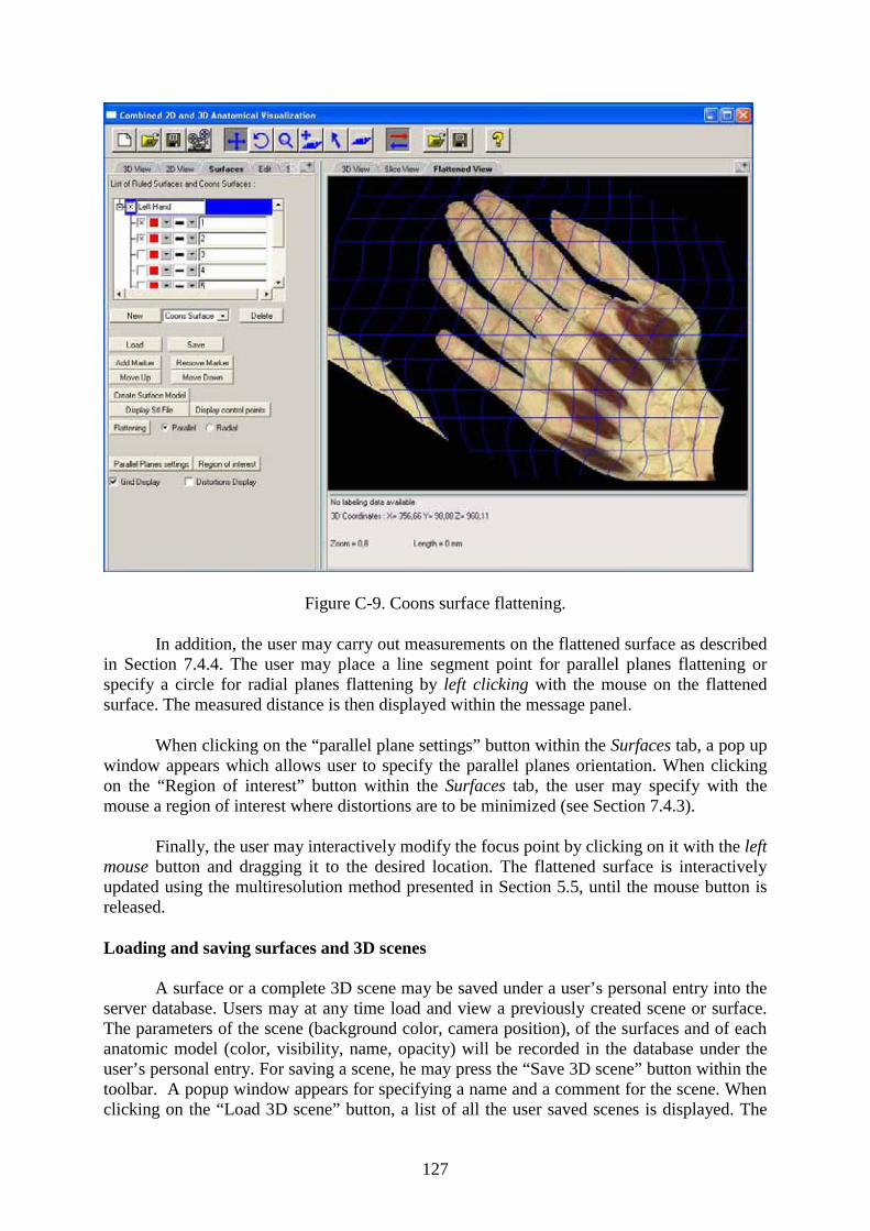
127
Figure C-9. Coons surface flattening.
In addition, the user may carry out measurements on the flattened surface as described in Section 7.4.4. The user may place a line segment point for parallel planes flattening or specify a circle for radial planes flattening by left clicking with the mouse on the flattened surface. The measured distance is then displayed within the message panel.
When clicking on the “parallel plane settings” button within the Surfaces tab, a pop up window appears which allows user to specify the parallel planes orientation. When clicking on the “Region of interest” button within the Surfaces tab, the user may specify with the mouse a region of interest where distortions are to be minimized (see Section 7.4.3).
Finally, the user may interactively modify the focus point by clicking on it with the left mouse button and dragging it to the desired location. The flattened surface is interactively updated using the multiresolution method presented in Section 5.5, until the mouse button isreleased.
Loading and saving surfaces and 3D scenes
A surface or a complete 3D scene may be saved under a user’s personal entry into the server database. Users may at any time load and view a previously created scene or surface. The parameters of the scene (background color, camera position), of the surfaces and of each anatomic model (color, visibility, name, opacity) will be recorded in the database under the user’s personal entry. For saving a scene, he may press the “Save 3D scene” button within the toolbar. A popup window appears for specifying a name and a comment for the scene. When clicking on the “Load 3D scene” button, a list of all the user saved scenes is displayed. The

128
user may then load the scene of its choice. For saving a surface, he may press the “Save surface” button within the Surfaces tab. As for a 3D scene, a popup window appears for specifying a name and a comment for the surface. When clicking on the “Load surface”button, a list of all the user saved surfaces is also displayed. The user may then load the surface of its choice.
Recording an animation
The applet allows a user to record a succession of actions within the 3D viewer such as navigation (rotation, zooming, translation), slice translation, display of curved surfaces or modification of the parameters of the anatomic models. This succession of actions enables then the creation of a corresponding video file. To record the actions, he may click on the “Video” button within the toolbar. The animation starts to be recorded immediately. Then, he may carry out his animation actions (maximum time : 3 minutes) and click again on the “Video” button to end recording the animation. A new window appears where he can write a name and a comment for the recorded animation.
To create the corresponding video animation, the user must go on the Visible Human web site and click on the item “Saved markers, 3D scenes and 3D animations”. In the folder “Your 3D scenes” he may locate the animation that has been saved and click on the button “Create”. The animation will be created in AVI format and will be available for downloading from the website.
129
References
[Achenbach et. al. 1998] S. Achenbach, W. Moshage, D. Ropers, and K. Bachmann, “Curved Multiplanar Reconstructions for the Evaluation of Contrast-Enhanced Electron-Beam CT of the Coronary Arteries,” Am. J. Roentgenol., pp. 895–899, 1998.
[Ackerman 1998] M. Ackerman, “The Visible Human Project,” Proc. of the IEEE,Vol. 86, No 3, pp. 504-511, 1998.
[Addis et. al. 2001] K. Addis, K. Hopper, T. Iyriboz, Y. Liu, S. Wise, C. Kasales, J. Blebea, and D. Mauger, “CT Angiography: In Vitro Comparison of Five Reconstruction Methods”, Am. J. Roentgenol., pp. 1171–1176, 2001.
[Alliez et. al. 2002] Alliez, P., Meyer, M., And Desbrun, M. 2002. Interactive Geometry Remeshing. ACM Transactions On Graphics (Siggraph 2002), Vol. 21, No 3, 347–354, 2002.
[Bennis et. al. 1991] C. Bennis, J.M. Vézien and G. Iglésias, “Piecewise Surface Flattening For Non-distorted Texture Mapping,” SIGGRAPH´91, Computer Graphics, Vol. 25, No 4, pp. 237-246, 1991.
[Bessaud and Hersch 2000] J.-C. Bessaud and R.D. Hersch, “The Visible Human Slice Sequence Animation Web Server,” The Third Visible Human Project Conference Proceedings, Bethesda, Maryland, October 2000.
[Brodlie and Wood 2001] K. Brodlie and J. Wood, “Recent Advances in Volume Visualization”, Computer Graphics Forum, Vol. 20, No 2, June 2001.
[Cohn 1980] H. Cohn, Conformal Mapping on Riemann Surfaces, Dover Publications, Inc., 1980, ISBN 0-486-64 025-6.
[Eck et. al. 1995] M. Eck, T. D. DeRose, T. Duchamp, H. Hoppe, M. Lounsbery, and W. Stuetzle, “Multiresolution analysis of arbitrary meshes,” Proc. of SIGGRAPH '95, pp. 173-182, 1995.
[Evesque et al. 2002] F. Evesque, S. Gerlach, and R.D. Hersch, “Building 3D Anatomical Scenes on the Web,” Journal of Visualization and Computer Animation,Vol. 13, pp. 43-52, 2002.
130
[Farin 1990] G. Farin, Curves and Surfaces for Computer Aided Geometric Design,second edition, Academic Press, Inc., 1990, ISBN 0-12-249051-7.
[Figueiredo and Hersch 2002] O. Figueiredo and R.D. Hersch, “Parallel Unfolding and Visualization of Curved Surfaces Extracted from Large 3D Volumes,” Journal of Electronic Imaging, Vol. 11, No 4, pp. 423-433, Oct. 2002.
[Floater 1997] M. Floater, “Parametrization and Smooth Approximation of Surface Triangulations,” Computer Aided Geometric Design, Vol. 14, No 3, pp. 231–250, April 1997.
[Floater and Hormann 2004] M. S. Floater and K. Hormann, “Surface Parameterization: a Tutorial and Survey,” Advances on Multiresolution in Geometric Modelling, N. Dodgson, M. S. Floater, and M. Sabin (eds.), Springer-Verlag, Heidelberg, pp. 157-186, 2004.
[Gering et al. 1999] Gering, D., Nabavi, A., Kikinis, R., Grimson, W., Hata, N., Everett, P., Jolesz, F., Wells, W., “An Integrated Visualization System for Surgical Planning and Guidance using Image Fusion and Interventional Imaging,” Proc. of the Second International Conference on Medical Image Computing and Computer-Assisted Intervention (MICCAI),Springer Verlag, pp. 809-819, 1999.
[Gerlach and Hersch 2002] S. Gerlach and R.D. Hersch, “A Real-Time Navigator For The Visible Human,” IEEE Internet Computing, Vol. 6, No 2, pp. 27-33, 2002.
[Golland et. al. 1999] P. Golland, R. Kikinis, M. Halle, C. Umans, W.E.L. Grimson, M.E. Shenton, J.A. Richolt, “AnatomyBrowser: A Novel Approach to Visualization and Integration of Medical Information,” Journal of Computer Assisted Surgery, Vol. 4, pp. 129-143, 1999.
[Haker et. al. 1999] S. Haker, S. Angenent, A. Tannenbaum and R. Kikinis, “On the Laplace-Beltrami Operator and Brain Surface Flattening,” IEEE Transactions on Medical Imaging, Vol. 18, pp. 700-711, 1999.
[Haker et. al. 2000] S. Haker, S. Angenent, A. Tannenbaum and R. Kikinis, “Non Distorting Flattening For Virtual Colonoscopy,” Third International Conference On Medical Robotics, Imaging and Computer Assisted Surgery,Pittsburgh, Pennsylvania, USA, 2000.
[He et. al. 2001] S. He, R. Dai, B. Lu, C. Cao, H. Bai, and B. Jing, “Medial Axis Reformation: A New Visualization Method For CT Angiography,” Academic Radiology, Vol. 8, pp. 726-733, 2001.
[Hersch et. al. 2000] R.D. Hersch, B. Gennart, O. Figueiredo, M. Mazzariol, J. Tarraga, S. Vetsch, V. Messerli, R. Welz, L. Bidaut, “The Visible Human Slice Web Server: A first Assessment,” Proc. of IS&T/SPIE Conference on Internet Imaging, San Jose, USA, Jan. 2000, SPIE Vol. 3964, pp. 253-258, 2000.
131
[Hoschek and Lasser 1993] J. Hoschek, AND D. Lasser , Fundamentals of Computer Aided Geometric Design, AK Peters, pp. 371-387, 1993.
[Kanitsar et. al. 2001] A. Kanitsar, R. Wegenkittl, P. Felkel, D. Fleischmann, D. Sandner, and E. Groller, “Computed Tomography Angiography: A Case Study of Peripheral Vessel Investigation,” Proc. of IEEE Visualization 2001,pp. 477–480, 2001.
[Kanitsar et. al. 2002] A. Kanitsar, D. Fleischmann, R. Wegenkittl, P. Felkel, and M.E. Gröller, “CPR - Curved Planar Reformation,” Proc. of IEEE Visualization 2002 (Vis02), IEEE Press, pp. 37-44, 2002.
[Kanitsar et. al. 2003] A. Kanitsar, D. Fleischmann, R. Wegenkittl, P. Felkel, and M.E. Gröller, “Advanced Curved Planar Reformation: Flattening of Vascular Structures,” Proc. of IEEE Visualization 2003 (Vis03), IEEE Press, pp. 43-50, 2003.
[Khodakovsky et. al. 2003] A. Khodakovsky, N. Litke, and P. Schroder, “Globally Smooth Parameterizations with Low Distortion,” ACM Transactions on Graphics (SIGGRAPH 2003), Vol. 22, No 3, pp. 350–357, 2003.
[Koenderink and Van Doorn 1992] JJ. Koenderink and A.J. Van Doorn, “Surface Shape and Curvature Scales,” Image and Vision Computing, Vol. 10, No 8, pp. 557–565, 1992.
[Kreyszig 1991] E. Kreyszig, Differential Geometry, Dover Publications, Inc., ISBN 0-486-66 721-9, 1991.
[Lee et. al. 1998] W. F. Lee, W. Sweldens, P. Schroder, L. Cowsar, and D. Dobkin, “MAPS: Multiresolution Adaptive Parameterization of Surfaces,” Proc. of SIGGRAPH 98, ACM Press, pp. 95-104, 1998.
[Levy and Mallet 1998] B. Levy and J. L. Mallet, “Non-Distorted Texture Mapping For Sheared Triangulated Meshes,” Proc. of ACM SIGGRAPH 98, ACM Press, pp. 343-352, 1998.
[Levy et. al. 2002] B. Levy, S. Petitjean, N. Ray and J. Maillot, “Least Squares Conformal Maps for Automatic Texture Atlas Generation,” Proc. of SIGGRAPH’02, 2002.
[Lorensen and Cline 1987] W.E. Lorensen and H.E. Cline, “Marching cubes : A High Resolution 3D Surface Reconstruction Algorithm,” Proc. ofSIGGRAPH 1987, ACM press, Vol. 21, No 4, pp. 163–169, 1987.
[Maillot et. al. 1993] J. Maillot, H. Yamia, and A. Verroust, “Interactive Texture Mapping,” Proc. of SIGGRAPH 1993, pp. 27–34, 1993.
[Meißner et. al. 2000] M. Meißner, J. Huang, D. Bartz, K. Mueller, R. Crawfis, “A Practical Evaluation of Popular Volume Rendering Algorithms,” Proc. of the 2000 IEEE symposium on Volume visualization, pp. 81-90, 2000.
132
[Mlejnek et. al. 2004] M. Mlejnek, A. Vilanova, M. E. Gröller, “Interactive Thickness Visualization of Articular Cartilage,” Proc. of Visualization 2004 (Vis04), IEEE Press, pp. 521-527, 2004.
[Mroz et. al. 2000] L. Mroz , H. Hauser, E. Gröller, “Interactive High-Quality Maximum Intensity Projection,” Proc. of Eurographics 2000, pp. 341-350, 2000.
[Napel et. al. 1992] S. Napel, M. P. Marks, G. D. Rubin, M. D. Dake, C. H. McDonnell, S. M. Song, D. R. Enzmann, and R. B. Jeffrey, “CT Angiography with Spiral CT and Maximum Intensity Projection,” Radiology 185,pp. 607-610,1992.
[North et. al. 1996] C. North, B. Schneiderman, C. Plaisant, “User Controlled Overviews of an Image Library: The Visible Human Explorer,” The Visible Human Conference Proceedings, October 1996.
[Pearson et. al. 1990] F. Pearson, B. Nordenskjold and T. J. Lam, Map Projections: Theory and Applications, CRC Press, ISBN 0-849-36888-X, 1990.
[Pinkall and Polthier 1993] U. Pinkall and K. Polthier, “Computing Discrete Minimal Surfaces and Their Conjugates”, Experimental Mathematics, Vol. 2, No 1, pp. 15-36, 1993.
[Poliakov et. al. 2001] A. Poliakov, E. Albright, D. Corina, G. Ojemann, R. F. Martin and J. F. Brinkley, “Server-based Approach to Web Visualization of Integrated 3-D Medical Image Data,” Proc. of AMIA'2001, 2001.
[Polthier and Schmies 1999] K. Polthier and M. Schmies, “Geodesic Flow on Polyhedral Surfaces,” Proc. of the Joint Eurographics and IEEE TCVG Symposium on Visualization 1999, pp. 179-188, 1999.
[Ralston and Rabinowitz 1978] A. Ralston, P. Rabinowitz, “First Course on Numerical Analysis,” McGraw-Hill, pp. 483-485, 1978.
[Richtsmeier et. al. 2002] J. T. Richtsmeier, V. B. Deleon, S. R. Lele, “The Promise of Geometric Morphometrics,” in Yearbook of Physical Anthropology,Vol. 45, pp. 63-91, 2002.
[Rossnick et al. 1986] S. Rossnick, D. Kennedy, G. Laubl, “Three Dimensional Display of Blood Vessels in MRI,” IEEE Computer in Cardiology, pp. 193–196, 1986.
[Rubin et. al. 2001] G. Rubin, A. Schmidt, L. Logan, and M. Sofilos, “Multi-Detector Row CT Angiography of Lower Extremity Arterial Inflow and Runoff: Initial Experience,” In Radiology 2001, pp. 146–158, 2001.
[Sander et. al. 2001] P. Sander, J. Snyder, S.J. Gortler, and H. Hoppe, “Texture Mapping Progressive Meshes,” Proc. of SIGGRAPH 2001, pp. 409–416, 2001.
133
[Saroul et. al. 2003] L. Saroul, S. Gerlach and R.D. Hersch, “Exploring Curved Anatomic Structures with Surface Sections,” Proc. of IEEE Visualization 2003(Vis03), IEEE Press, pp. 27-34, 2003.
[Saroul et. al. 2004] L. Saroul, S. Gerlach and R.D. Hersch, “Interactive Specification and Extraction of Free Form surfaces from the Visible Human,” Internet Imaging V, Proceedings of the SPIE, Vol. 5304, pp. 242-253, January 2004.
[Saroul et. al. 2006] L. Saroul, O. Figueiredo and R.D. Hersch, “Distance Preserving Flattening of Surface Sections”, IEEE Transactions On Visualization and Computer Graphics (TVCG), Vol. 12, No. 1, pp. 26-35, 2006.
[Schubert et. al. 1999] R. Schubert, B. Pflesser, A. Pommert, K. Priesmeyer, M. Riemer, T. Schiemann, U. Tiede, P. Steiner, and K. H. Höhne, “Interactive Volume Visualization using Intelligent Movies,” in Medicine meets Virtual Reality, Proc. MMVR '99 (J. D. Westwood, et. al. eds.), Vol. 62 of Health Technology and Informatics, Amsterdam: IOS Press, pp. 321-327, 1999.
[Sheffer and de Sturler 2001] A. Sheffer and E. de Sturler, “Parameterization of Faceted Surfaces for Meshing using Angle Based Flattening,” Engineering with Computers, Vol. 17, No 3, pp. 326-337, 2001.
[Sheffer et. al. 2005] A. Sheffer, B. Levy, M. Mogilnitsky and A. Bogomyakov, “ABF++ Fast and Robust Angle Based Flattening,” ACM Transactions on Graphics,ACM Press, Vol. 24, No 2, pp. 311-330, April 2005.
[Sorkine et. al. 2002] O. Sorkine, D. Cohen-Or, R. Goldenthal and D. Lischinsky, “Bounded-distortion Piecewise Mesh Parameterization,” Proc. of IEEE Visualization 2002 (Vis02), IEEE Press, pp. 355-362, 2002.
[Spiegel 1963] M. R. Spiegel, Advanced Calculus, Schaum’s Outline Series, McGraw-Hill, Chapter 8, p. 164, 1963.
[Wang et. al. 2003] Y. Wang, B. S. Peterson, and L. H. Staib, “3D Brain Surface Matching Based on Geodesics and Local Geometry,” Computer Vision and Image Understanding, Vol. 89, pp. 252-271, 2003.
[Warrick and Funnell 1998] P.A Warrick, W.R.J. Funnell, “A VRML-based Anatomical Visualization Tool for Medical Education,” IEEE Transactions on Information Technology in Biomedicine, Vol. 2, No. 2, pp. 55-61, 1998.
[Welch and Witkin 1994] W. Welch and A. Witkin, “Free-Form Shape Design Using Triangulated Surfaces,” Proc. of SIGGRAPH 1994, pp. 247-256, 1994.
[Wyvill et. al. 1986] B. Wyvill, C. McPheeters, G. Wyvill, “Soft Objects,” in Advanced Computer Graphics, Proceedings of Computer Graphics International,pp. 113-128, Tokyo 1986.

134
[Zigelman et. al. 2002] G. Zigelman, R. Kimmel and N. Kiryati, “Texture Mapping Using Surface Flattening via Multidimensional Scaling,” IEEE Transactions on Visualization and Computer Graphics, Vol. 8, No 2, pp. 198-207, 2002.
135
Biography
Laurent Saroul was born on July 21st, 1978, in Valence, France. He graduated in 2001 as an Electronics and Physics engineer from CPE-Lyon, a French engineering school located in Lyon, France. He received the same year a Master degree in image processing and computer graphics from Université Jean Monnet, St-Etienne, France. Since 2002, he works at the Peripheral Systems Laboratory of the Ecole Polytechnique Fédérale de Lausanne, Switzerland as a research assistant and PhD candidate. His current research interests include image processing, computer graphics and volume visualization techniques.
His past professional experience includes:
• Institut National de Recherche en Informatique et Automatique (INRIA Paris, France) in 2001: Research on image processing tools for the automatic segmentation of clouds within satellite images. Development of an image processing software.
• Pôle Européen de Plasturgie (Oyonnax, France), 2000: Conception and development of a data acquisition system. Development of a Labview software.
Publications
• L. Saroul, S. Gerlach and R.D. Hersch, “Exploring Curved Anatomic Structures with Surface Sections,” Proc. of IEEE Visualization 2003 (Vis03), IEEE Press, pp. 27-34, 2003.
• L. Saroul, S. Gerlach and R.D. Hersch, “Interactive Specification and Extraction of Free Form surfaces from the Visible Human,” Internet Imaging V, Proceedings of the SPIE, Vol. 5304, pp. 242-253, January 2004.
• L. Saroul, O. Figueiredo and R.D. Hersch, “Distance Preserving Flattening of Surface Sections”, IEEE Transactions On Visualization and Computer Graphics (TVCG), Vol. 12, No. 1, pp. 26-35, 2006.