Embed Size (px)
Citation preview

SURFACE CAPTURE USING NEAR-REAL-TIME
PHOTOGRAMHETRY FOR A COMPUTER
NUMERICALLY CONTROLLED HILLING SYSTEM
Reto Wildschek, B.Sc (Eng), Cape Town
April 1999
Submitted to the University of Cape Town
in partial fulfilment for the degree of
Master of Science in Engineering.
. • • . •. . • .... , C•'.• ,,,.,-. ,, .• ,~.:;:;,=;·"'°"'"""'~---- ·~···ri
· .. :" ·· '·v r' ('··•A T•r,·n has been given,.\ · :~:_· ·; ;~.· -~ :-,:; .. 1~~ ;~.; ·i;;~;~ 1-b~.~.is in ~-,hole !]i ....•... •• ..... , •' ( io 1'·cid b· 1~'·"' author ·1 • - • 1,. • ...... -- "I ~·· 1.. v ~ ' I "'""' •
' .-·.-·. ~-·-····...,... .. ·.~·'.::·.~,·:·: ... ·:::o·-.o~,~~-;._,. ~ ·"---'--•~

The copyright of this thesis vests in the author. No quotation from it or information derived from it is to be published without full acknowledgement of the source. The thesis is to be used for private study or non-commercial research purposes only.
Published by the University of Cape Town (UCT) in terms of the non-exclusive license granted to UCT by the author.

I, Reto Wildschek, submit this thesis in partial fulfilment of the
requirements for the degree of Master of Science in Engineering.
I affirm that this is my original work and that it has not been
submitted in this or a similar form for a degree at any
University.

- i -
ABSTRACT
During the past three years, a research project has been carried
out in the Department of Mechanical Engineering at UCT, directed
at developing a system to accurately reproduce three-dimensional
(3D), sculptured surfaces on a three axis computer numerically
controlled (CNC) milling machine. Sculptured surfaces are surfaces
that cannot easily be represented mathematically. The project was
divided into two parts: the development of an automatic non
contact 3D measuring system, and the development of a milling
system capable of machining 30 sculptured surfaces (Back, 1988).
The immediate need for such a system exists for the manufacture
of medical prostheses.
The writer undertook to investigate the measurement system, .with
the objective to develop a non-contact measuring system that can
be used to 'map' a sculptured surface so that it can be
represented by a set of XYZ coordinates in the form required by
the milling system developed by Back (1988).
This thesis describes the development of a PC-based near-real
time photogrammetry system (PHOENICS) for surf ace capture. The
topic is intoduced by describing photogrammetric principles as
used for non-contact measurements of objects.
A number of different algorithms for image target detection,
centering and matching is investigated. The approach to image
matching adopted was the projection of a regular grid onto the
surface with subsequent matching of conjugate grid intersections.
A general algorithm which automatically detects crosses on a line
and finds their accurate centre~ was developed. This algorithm
was then extended from finding the crosses on a line, to finding
all the intersection points of a grid. The algorithms were
programmed in TRUE BASIC and specifically adapted for use with
PHOENICS as an object point matching tool.

- ii -
The non-contact surface measuring technique which was developed
was used in conjunction with the milling system developed by
Back (1988) to replicate a test object. This test proved that the
combined system is suitable for the manufacture of sculptured
surf aces.
The accuracy requirements for the manufacture of medical
prostheses can be achieved with the combined measuring and
milling system. At an object-to-camera distance of 0.5 m, points
on a surface can be measured with an accuracy of approximately
0.3 mm at an interval of 5 mm. This corresponds to a relative
accuracy of 1:1600. Back (1988) reported an average undercutting
error of 0.46 mm for the milling system. This combines to an
uncertainty of 0.55 mm.
Finally, the limitations of PHOENICS at its prototype stage as a
surface measuring tool are discussed, in particular the factors
influencing the system's accuracy. PHOENICS is an ongoing project
and the thesis is concluded by some recommendations for further
research work.

- iii -
ACKNOWLEDGEMENTS
The author would like to gratefully acknowledge the contribution
of the following:
My supervisor, Mr. Andrew Sass, for his help and guidance,
My supervisor, Assoc. Prof. Heinz RUther, for his continual
encouragement and in~est, and who was always willing to give of
his time,
Mr. Nicky Parkyn and Assoc. Prof. Heinz RUther, for the use of
their computer programs,
The CSIR, for their financial assistance,
The staff of the Surveying Department.

iv
CONTENTS
. . . . . . . . . . . . . . . . . . . . . . . . . . . . . . . . . . . . . . ABSTRACT
ACKNOWLEDGEMENTS
LIST OF ILUSTRATIONS
. . . . . . . . . . . . . . . . . . . . . . . . . . . . . . . . . . . . . . . . . . . . . . . . . . . . . . . . . . . . . .
Page
• • • i
iii
viii
1.0 INTRODUCTION . . . . . . . . . . . . . . . . . . . . . . . . . . . . . . . . . . . . . . . 1
2.0 PHOTOGRAMMETRY . . . . . . . . . . . . . . . . . . . . . . . . . . . . . . . . . 2.1
2.2
Introduction
Applications
and Definition . . . . . . . . . . . . . . . . . . . . . . . . . . . . . . . . . . . . . . . . . . . . . . . . . . . . . .
2.3 Basic Geometry of the Single Photograph ·······~·
2.3.1 Projections ••••••••••••••••••••••••• ..•••••.
2.3.2 Image and Object Space ••••••••••••••••••••••
2.3.3 Interior Orientation ••••••••••••••••••••••••
2 • 3 • 4 Ext 9· r i o r O r i e n tat i on • • • • • • • • • • • • • • • • • • • • • • • •
2.3.5 The Collinearity Condition ••••••••••••••••••
2.4 Obtaining the Third Dimension from Two
Overlapping Photographs •••••••••••••••••••••••••
2.5 Projective Transformation Restitution of
the Object ••••••••.•••••••••••.•••.•••••.•.•.••.
3.0 DEVELOPMENT OF A PC-BASED NRTP SYSTEM . . . . . . . . . . . . .
4.0 IMAGE AQUISITION WITH CCD CAMERAS . . . . . . . . . . . . . . . . . 4.1
4.2
The Vidicon Camera Tube •••••••••••••••••••••••••
Solid State Sensors •••••••••••••••••••••••••••••
4.3 CCD Cameras . . . . . . . . . . . . . . . . . . . . . . . . . . . . . . . . . . . . . 4.3.1
4.3.2
Interline VS Frame Transfer . . . . . . . . . . . . . . . . . CCD
4.4 CCD vs
Performance
Vidicon Tube
Features
Cameras
.................. ·-· . . . . . . . . . . . . . . . . . . . . .
7
7
12
14
14
16
17
17
18
20
22
25
32
33
35
36
38
41
42

v
Page
5.0 A REVIEW OF IMAGE MATCHING AND NRTP SYSTEMS . . . . . . . 5.1
5.2
5.3
5.4
5.5
5.6
5.7
5.8
5.9
6.0
Isis Scanner ······~····•••••••••••••••••••••••••
Mapvision •••••••••••••••••••••••••••••••••••••••
A RTP System for Object Measurement at the
National Research Council of Canada ••••••••••
A Close-Range Mapping System at the University
of Illinois •...•.•••..•....•••••••.....•.•••....
Robot Vision at the National Research Council
of Canada ••••••••••••••••••••••••••••.••••••
Rasterstereography ••••••••••••••••••••••••••••••
A System for Capturing Facial Surface
Information at the University of Minesota •••••••
Digital Image Correlation •••••••••••••••••••••••
Conclusions ....••••.......•..•............... ·~·.
DEVELOPING AN AUTOMATIC IMAGE TARGET DETECTION AND
. . . . . . . . . . . . . . . . . . . . . . . . . . . . . . . . MATCHING ALGORITHM
6.1 Problem Formulation . . . . . . . . . . . . . . . . . . . . . . . . . . . . . 6.1.1
6 .1. 2
6.1.3
6.1.4
Problem Statement . . . . . . . . . . . . . . . . . . . . . . . . . . . Requirements ••••••••••••••••••••••••••••••••
Constraints •••••••••••••••••••••••••••••••••
Criteria •••••••.••.••••..•.••.......•• • ....•
6.2 Concept Formation •••••••••••••••••••••••••••••••
6.2.1 Finding Corresponding Points •••••••••••••
6.2.2 Target Recognition and Centering ••••••••••••
6.2.3 Line Following ••••••••••••••••••••••••••••••
6.3 Summary and Conclusions . . . . . . . . . . . . . . . . . . . . . . . . . 7.0 DISCUSSION OF SOLUTION . . . . . . . . . . . . . . . . . . . . . . . . . . . .
7.1 A General Line Following and Cross Detection
Algorithm ••.••••••••••••••••••••••••••••••••••••
7.1.1 Line Detection ••••••••••••••••••••••••••••••
44
45
46
47
48
50
51
53
54
55
56
56
56
56
57
57
64
65
68
74
76
77
77
79

- vi
Page
7.1.2
7 .1. 3
Line Following and Cross Detection . . . . . . . . . . Accurate Cross Positioning . . . . . . . . . . . . . . . . . .
7.2 Cross Detection, Centering and Matching for
79
84
PHOENICS • • • • • • • • • • • • • • • • • • • • • • • • • • • • • • • • • • • • • • • • 86
a.o TESTING THE CROSS DETECTION AND CENTERING
ALGORITHM . . . . . . . . . . . . . . . . . . . . . . . . . . . . . . . . . . . . . . . . . 90
8.1 Precision of Finding a Cross in an Image •••••••• 90
8.1.1 Obtaining the First Approximation to the
Cross Centre •••••••••••••••••••••••••••••••• 90
8.2 Precision of Determining the Cross Centre ••••••• 91
8.3 Accuracy of Measuring a Surface ••••••••••••••••• 95
8.3.1 Choice of Test Surface and Control Field •••• 95
9.0
8.3.2
8.3.3
Surf ace Measurement with PHOENICS ............ • . Results of Measuring the Test Surface . . . . . . .
DISCUSSION OF THE ERRORS AND LIMITATIONS OF
PHOENICS . . . . . . . . . . . . . . . . . . . . . . . . . . . . . . . . . . . . . . . . . 9.1 Accuracy Limitations in Measuring a Surface
97
99
101
with PHOENICS •••••••••••••••••••••••••••••••••• 101
9.2 Limitations of Surface Measurement with
PHO ENI CS • • • • • • • • • • • • • • • • • • • • • • • • • • • • • • • • • • • • • • • 103
10.0 CONCLUSIONS AND RECOMMENDATIONS ••••••••••••••••• 106
10.1 Conclusions •••••••••••••••••••••••••••••••••• 106
10.2
10.3
Recommendations
Closing remarks
. . . . . . . . . . . . . . . . . . . . . . . . . . . . . .
. . . . . . . . . . . . . . . . . . . . . . . . . . . . . . 11.0 REFERENCES . . . . . . . . . . . . . . . . . . . . . . . . . . . . . . . . . . . . . . 12.0 BIBLIOGRAPHY . . . . . . . . . . . . . . . . . . . . . . . . . . . . . . . . . . . .
107
108
110
114

- vii -
APPENDICES Page
A. Derivation of the Orientation Matrix • • • • • • • • • • • • • • A- 1
B. Derivation of the Collinearity Condition . . . . . . . . . . c. Epipolar Geometry . . . . . . . . . . . . . . . . . . . . . . . . . . . . . . . . . D. A Method of Interfacing the PIP Image Processing
Board with a Computer Language other than those
it supports . . . . . . . . . . . . . . . . . . . . . . . . . . . . . . . . . . . . . . . E. Evaluation of Using the Weighted Hean Technique
for Determining the Position of a Line-Section
B-1
C-1
0-1
with Sub-Pixel Accuracy ••••••••••••••••••·······~· E-1 (')
F. List of Programs for Use with PHOENICS •••••••••••• F-1
F.1 TRUE BASIC Programs •••••••••••••••••••••••••• F-1
F.2 PIP Image Processor Macros ••••••••••••••••••• F-2
G. A Set of Typical Images which were used for
Surface Measurement with PHOENICS ••••••••••••••••• G-1
H. Coordinates of the Control Frame •••••••••••••• ~ ••• H-1
I. Sample Output of Photogrammetric Software for the
Test Sphere . . . . . . . . . . . . . . . . . . . . . . . . . . . . . . . . . . . . . . . I-1

- viii
LIST OF ILLUSTRATIONS
FIGURES Page
1 • 1
2.1
2.2a
2.2b
2.3
t.4
2.5
2.6
2.7
2.0
2.9
3.1
3.2
3.3
4.1
4.2
4.3
4.4
5.1
s.2 S.3
S.4
6.1
6.2
Mathematically generated surface which was
machined with the milling system •••••••••••••••••• 3
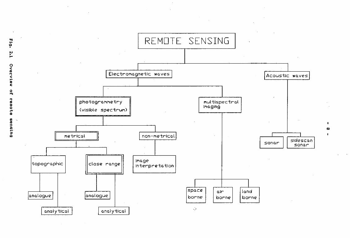
Overview of remote sensing •••••••••••••••••••••••• 8
Relative orientation ••••••••••••••••••••••••••••• 10
Absolute orientation ••••••••••••••••••••••••••••• 11
Orthographic projections ••••••••••••••••••••••••• lS
Perspective projections •••••••••••••••••••••••••• lS
Image and object space ••••••••••••••••••••••••••• 16
Interior orientation . . . . . . . . . . . . . . . . . . . . . . . . . . . . . Exterior orientation by omega, phi and kappa · •••••
-Collinearity condition •••••••••••••••••••••••••••
Geometry of two overlapping photographs •· . . . . . . . . .
Schematic of PHOENICS hardware configuration •••••
PHOENICS hardware ••••••••••••••••••••••••••••••••
Control point target design for PHOENICS . . . . . . . . . Vidicon camera tube ••••••••••••••••••••••••••••••
CCD MOS strucure •••••••••••••••••••••••••••••••••
. . . . . . . . . . . . . . . . . . . . . . . . Interline charge transfer
Frame charge transfer . . . . . . . . . . . . . . . . . . . . . . . . . . . . Principle of operation of the Isis Scanner •••••••
Image correlation along epipolar lines •••••••••••
Optical beam defle~tion assembly •••••••••••••••••
Cross- and line rasterstereography •••••••••••••••
Example of a grey image ••••••••••••••••••••••••••
Pixel intensities of a grey image ••••••••••••••••
17
18
19
20
27
28
31
33
37
38
39
45
49
so S2
S9
60

ix
FIGURES Page
6.3
6.4
6.5
6.6
6.7
6.8
6.9
6.10
6.11
6.12
7.1
7.2
7.3
7.4
7.5
7.6
8.1
8.2
8.3
A.1
Thresholding . . . . . . . . . . . . . . . . . . . . . . . . . . . . . . . . . . . . . Example of a binary image ••••••••••••••••••••••••
Pixel intensities of a binary image ••••••••••••••
The pixeling effect ••••••••••••••••••••••••••••••
Grids for object targeting . . . . . . . . . . . . . . . . . . . . . . . Circular targets . . . . . . . . . . . . . . . . . . . . . . . . . . . . . . . . . Cross centering with higher order moments ••••••••
Modelling a cross as the intersection of two
lines . . . . . . . . . . . . . . . . . . . . . . . . . . . . . . . . . . . . . . . . . . . . Modelling a cross as the intersection of two line
61
62
63
64
67
70
71
72
segments ··~··•••••••••••••••••••••••••••••••••••••73
Line following using a search-circle •••••• ~ •••••• 75·
line following and Flow diagram of a general
cross detection algorithm . . . . . . . . . . . . . . . . . . . . . . . . Search-circle used for line following and cross
detection . . . . . . . . . . . . . . . . . . . . . . . . . . . . . . . . . . . . . . . . Line and circle configurations characteristic of
the number of search-circle intersections found
Finding the first approximation to the points on
. .
78
80
81
the lines which form a cross ••••••••••••••••••••• 84
Determining the position of the centre of the
line to sub-pixel accuracy . . . . . . . . . . . . . . . . . . . . . . . 85
Cross detection, centering, and matching with
PHOENICS . . . . . . . . . . . . . . . . . . . . . . . . . . . . . . . . . . . . . . . . . 87
Pixel intensity profiles across two typical
lines . . . . . . . . . . . . . . . . . . . . . . . . . . . . . . . . . . . . . . . . . . . . 94
Control frame and test surface ••••••••••••••••••• 96
Surface measurement with PHOENICS •••••••••••••••• 98
Three-dimensional right-handed coordinate
system . . . . . . . . . . . . . . . . . . . . . . . . . . . . . . . . . . . . . . . . . . A-1

- K
FIGURES Page
8.1
8.2
c.1
Diagram of the collinearity condition . . . . . . . . . . . Image coordinate system rotated so that it is
parallel to the object space . . . . . . . . . . . . . . . . . . . . Epipolar plane and epipolar lines . . . . . . . . . . . . . . .
8-1
8-2
C-1
E.1 Pixel intensity profiles of two typical line
sections . . . . . . . . . . . . . . . . . . . . . . . . . . . . . . .. . . . . . . . . . E-2
G.1 Grey image (left) for determining the control
points ....•......•.•......•................ -..... G-2
G.2 Thresholded image (left) for determining the
con'tol points . . . . . . . . . . . . . . . . . . . . . . . . . . . . . . . . . . . G-3
G.3 Grey image (left) for determining the object
points . . . . . . . . . . . . . . . . . . . . . . . . . . . . . . . . . . . . . . . . . . G-4
G. 4 Thresholded image (left) for determining the
object points . . . . . . . . . . . . . . . . . . . . . . . . . . . . . . . . . . . G-5
G.5 Grey image (right) for determining the control
points ..•..•.•.•...•.•...•......•............... G-6
G.6 Grey image (right) for determining the object
points ........•.....•....•...................... G-7
G.7 Image for determining the object points with a
graduated grid overlayed . . . . . . . . . . . . . . . . . . . . . . . . G-8
H .1 Numbering of control frame . . . . . . . . . . . . . . . . . . . . . . H-2

- xi -
TABLES Page
8.1 Maximum dev.ations in x and y of the calculated
8.2
cross position from the mean cross centre
Results of measuring the test sphere with
. . . . . . . . PHOENICS ••••••••••••••••••••••••••••••••••••••••
E.1 Pixel intensity values of two typical line
92
100
sections •...•......•.....•..•••.•.......•....... E-1
E.2 Results of applying the weighted mean technique
for finding the position of a line section . . . . . . E-3
H .1 Coordinates of control frame • • • • • • • • • • • • • • • • • • • • H·- ·1

- 1 -
CHAPTER ONE
1.0 INTRODUCTION
During the past three years, a research project has been carried
out in the Department of Mechanical Engineering at UCT, directed
at developing a system to accurately reproduce three-dimensional
(3D), sculptured surfaces on a three axis computer numerically
controlled (CNC) milling machine. Sculptured surfaces are surfaces
that cannot easily be represented mathematically. Duncan and
Hair (1983) describe these surfaces as "those surface shapes which
cannot continuously be generated and have the arbitrary or
complex character of forms traditionally modelled by sculptors".
The need for the system arose because the Biomedical Engine~ing
department wanted to produce prostheses such as shoe inserts and
sockets for amputee stumps efficiently and quickly. They wanted
a non-contacting measuring system to accurately measure, for
example, the stump of an amputee or a deformed foot with as
little patient discomfort as possible. These measurements are
then to be used to machine either a positive or a negative image
of the surf ace.
The first design was undertaken by Berelowitz in 1986 as an
undergraduate thesis. Berelowi tz (1986) used a digital camera
called a 'TopoScanner' (Vaughn, Brooking, Price and Ireland, 1983)
to capture the surface topography, an IBM PC microcomputer for
data processing, and a three axis CNC milling machine to
manufacture the surface. The dataprocessing included fitting a
surf ace through the points measured by the TopoScanner,
calculating the toolpath for the cutter, and translating the
latter into instructions for the CNC machine. A punched paper
tape was then produced to transfer the data to th• CNC milling
machine and the part milled.

- 2 -
Berelowi tz (1986) produced a system with a great deal of potential
but with limited accuracy. Back (1988) in an H.Sc thesis, set out
to improve Berelowitz's design. He found fundamental problems
with the TopoScanner and with certain assumptions in the surface
fitting algorithms. Secondly, communication between the IBH PC
and the CNC machine via the large amounts of paper tape were
cumbersome. It also became clear that the complete system was
too large a task for a single H.Sc thesis, so the task was
divided into two parts; the measurement system and the milling
system.
Back successfully:
developed a mathematical algorithm to approximate a
sculptured surface represented by a set of surface
datapoints in the form of XYZ coordinates. These
datapoints can either be measured from an existing surface
or calculated from a mathematical surface equation.
developed an algorithm to calculate the toolpath to
machine the sculptured surface.
wrote a computer program which displays the surface and
toolpath in three dimensions on the computer screen.
developed an algorithm which translates the toolpath into
a program suitable for use with the CNC machine.
developed a communications link for the direct transmission
of the CNC program from the IBH microcomputer to the
memory of the CNC computer.
The system is fully operational and was used to machine a variety
of surfaces. An example of a mathematically defined surf ace that
was produced is given in Fig. 1.1.
An indication of the accuracy of the milling system was obtained
by milling a mathematically generated test surf ace whose shape is
typical of that likely to be encountered by the milling system.
Analysis of the data revealed an average undercutting error of

- 3 -
0.46 mm ± 0.20 mm over the entire surface. Al though this error is
large in terms of conventional machining requirements, it is
acceptable tor the manufacture ot medical prostheses previously
described.
Fig. 1.1 Hathematically generated surf ace which was machined
with the milling system
The writer undertook to investigate the measurement system, with
the following objectives:
to develop a non-contact measuring system that can be
used to 'map' a sculptured surface so that it can be

- 4 -
represented by a set of XYZ coordinates in the form
required by the milling system developed by Back (1988).
to develop the system in such a way that it can serve as
an introduction to Computer Aided Design and Hanutacture
(CAD/CAM) for undergraduate students who wish to further
their studies in this specialised field.
The fundamental problems of the TopoScanner could not be
resolved, so alternative. methods were investigated.
Photogrammetry seemed the most appropriate technique to start
with as research work that appeared to have great potential, had
just been started in UCT's Department of Surveying. Various
hardware components had been purchased with the intentions to
ultimately develop a real-time photogrammetric (RTP) mapping
system. To th~ best of the writers knowledge, there are only 6 to
10 such systems operational worldwide - none on a microcompu~er.
Joining the research team in the Department of Surveying was
thought to be an ideal opportunity to attain the primary
objective and hence this path was followed.
In view of the above, a set of secondary objectives were
formulated.
1. Assist, in the development of the RTP system, in particular
the image matching algorithms.
2. Establish the feasibility of using the system for the
purpose of mapping a sculptured surf ace.
3. Select a test surface that can be defined mathematically
and check the matching algorithm for logic and accuracy.
4. If this data proves to be suitable, use it in the milling
program developed by Back (1989).

- s -
Thesis outline
Chapter 2 gives an overview of basic photogrammetry as this is a
specialised field of Surveying with which undergraduate and
graduate engineers are not usually familiar. The reader is
introduced to the terminology commonly used in this discipline
and an analytical approach for solving the photogrammetric
problem is presented.
Chapter 3 begins by giving the motivations for th~ development
of RTP systems. The design stages of such a RTP system are
discussed, and a-description is given of the near-real-time
photogrammetric (NRTP) system being developed at UCT.
As the advent of digital came~as has made possible the
developmen~ of RTP systems an introduction to the technologr of
these cameras is given in Chapter 4. The older Vidicon camera is
also described, and the two camera types are compared.
Chapter S gives a review of NRTP systems with reference to the
image matching algorithms used.
Chapter 6 discusses some of the concepts which were considered
for developing an automatic image target detection and matching
algorithm.
The image target detection and matching algorithm which was
developed is described in Chapter 7.
The developed algorithm was programmed and tested in two stages
on real image data. In Chapter 8 the two stages of testing are
described and the results that were obtained are presented.
In Chapter 9 the limitations of the non-contact surface
measuring technique which was developed, are discussed.

- 6 -
The final chapter outlines the conclusions which were drawn and
the recommendations that were made.

- 7 -
CHAPTER TWO
2.0 PHOTOGRAHHETR'i
2.1 Introduction and Definition
The word photogrammetry is derived from the three greek words,
photos meaning 'light', gramma meaning 'something drawn or
written', and matron meaning 'measurement'. Hence the original
meaning of the word is 'measuring graphically using light'. The
American Society of Photogrammetry (1980) defines photogrammetry
as:
"Photogrammetry is the art, science and technology of
obtaining reliable information about physical objects and
the environment through processes of recording, measuring,
and interpreting photographic images and patterns of
electromagnetic radiant energy and other phenomena."
Photogrammetry can be regarded as a branch of remote sensing
which in the broadest sense is the aquisition of some physical
property about an object without physical contact between it and
the mea~uring device. Photogrammetry in turn can be divided into
two categories: metrical photogrammetry and photo interpretation.
In general, the first category is concerned with determining the
relative locations of points in the space surrounding the object
or on the object so that distances, angles, areas, volumes,
elevations, the sizes and shapes of objects can be derived eg. a
topographic map. In photo interpretation, on the other hand,
photographs are evaluated qualitatively.
A diagramatic overview of remote sensing is given in Fig. 2.1.
l'SJ .... IQ • f\J • ....
0 < ID .., < .... ID c 0 ..., .., ID B 0 rt" ID
l1J ' ID :I l1J .... :I IQ
REMOTE
I ElectroMo.gnetlc wo.ves I
I photogro.MMetry
(visible spectruM)
l
I
II Metrlco.l ij I
I non-~etrlco.l j
I topogro.phic
~~-9ue]
I o.no.lyt1co.l I
l close ro.nge
~no.logue]
I o.no.lytlco.l
IMo.ge lnterpreto. tlon
SENSING
I spo.ce
borne
. '
Mul tlspectro.l IMo.glng
o.ir borne
l lo.nd borne
[Acoustic wo.ves I I
I
sono.r I I
slciesco.n I sono.r
CX>

- 9 -
As this thesis makes use of some of the tools and techniques
used in metrical photogrammetry, a brief overview has been
included •
. Metrical photogrammetry
Metrical photogrammetry can generally be seen to consist of
three stages:
1. Aquiring an image of the object to be measured.
2. Measuring the image of the object.
3. Extracting 30 information about the object from the
photographs from these measurements.
Besides using conventional photographic systems to perform Stage
1, other techniques such as radar imaging and X-ray imaging are
used. ;~.
Stages 2 and 3 can be accomplished by one of two methods. The
first method uses complex instrumentation and is thus known as
instrumental or analogue photogrammetry. A stereoscopic plotting
instrument, an opto-mechanical device of high precision, is used
to project and orientate two overlapping photographs in such a
way that a 30 model of the original object is formed. This
situation is created when all corresponding projected rays of the
two photographs intersect in space which in effect means the
reconstruction of the relative and absolute orientations of the
camera exposure stations from where the photographs were taken.
Relative orientation refers to the correct orientation in space
of the two projections with respect to one another (Fig. 2.2a).
Absolute orientation refers to the correct orientation and scale
of the model formed through the process of relative orientation
with respect to a reference ground system (Fig. 2.2b).

- 10 -
/
object
A IMa.ge pla.ne
perspective projec·t1ons of the object
reconstruction of rela. tlve orient a. t1on
Fiq. 2.2a Relative orientation
IMa.ge points
of object :'.

sea.le corrected
orlenta. tlon corrected
- 11 -
y
sea.led Model
z
sea.led Model
x
reconstruction of a.lo solute orlenta. tlon
Pig. 2.2b Absolute orientation

- 12 -
In instrumental photogrammetry, relative orientation may either
be accomplished empirically or numerically. In the first method
six rays passing through the two photographs are brought to
intersect in space in a repetitive, trial-and-error process. In
numerical relative orientation the adjustments required are
calculated from parallax measurements made with the stereoplotter
after the photographs have been placed into it. Absolute
orientation is then performed empirically by eliminating parallax
from three control points; points with known XYZ coordinates.
Subsequently, an operator can use the stereoplotter to produce a
topographic map or to obtain true XYZ coordinates of a number of
points on the model; this is known as a digital terrain model
(DTM).
The second method, analytical photogrammetry, uses less complex
but also very precise instrumentation. Measurements of x and,. y
coordinates of common image points are made on the overlapping
photographs with a comparator and used as input to a computer
program to determine relative and absolute orientation. A
mathematical model then used to determine the true XYZ
coordinates of the object from points on the photographs. From
this DTH a contour map can be produced.
The main difference between the instrumenntal method and the
analytical method is that the former relies on a very precise
mechanical system, whereas the latter uses an extensive
mathematical model to solve the photgrammetric problem.
Analytical photogrammetry is generally more accurate and easier
to operate and thus, stereoplotters are progressively being used
less and less.
2.2 Applications
Al though photogrammetry is still principally a surveyor's tool
used for the making of maps, especially topographic maps, it has

- 13 -
over the years found applications in many other scientific
disciplines. The rapid growth of application areas started at the
turn of the century when photogrammetry was first used in
architecture. This became known as close-range photogrammetry:
defined by some photogrammetrists as photogrammetry where the
object to camera distance is less than 300 metres. All of the
application areas mentioned below are examples of close-range
photogrammetry.
Applications in architecture include surveys of historical
monuments and sites as well as archaeological surveys. For
specific examples, the reader is referred to the proceedings of
the first International Symposium on Photogrammetric Surveys of
Monuments and Sites, Athens (Badekas, 1974).
Applications in Zoology range from mapping the beak of a Shoabill
(Adams, 1980) to measuring African Elephants (RUther, 1979).
Applications in the medical field are also many and varied. An
example is Dental-Stereophotogrammetry (Adams, 1978).
Another area which has numerous examples and a seemingly endless
growth of applications in close-range photogrammetry, is in the
industrial field. Today photogrammetry is used in building
construction, civil engineering, mining, vehicle and machine
construction, metallurgy, shipbuilding and many other areas. Some
of the advantages to be gained from using photogrammetry as a
measuring technique over conventional methods, are given by
Kntjdler and Kupka (1974) in their article on production of ship
propellers. These can be summarised as :
- time to measure the object is reduced by 90-95%.
- reduced material expenditure in the propeller casting
manufacture through optimized moulds.
- reduced machine time for blade machining through
optimization of the metal removal rate.

- 14 -
Kntidler and Kupke (1974) also report that the photogrammetric
technique "is equally suited for other industries where
workpieces of a compl~x surf~ce configuration are to be
manufactured, which would be very time consuming to measure with
conventional measuring tools".
2.3 Basic Geometry of the Single Photograph
As already mentioned there are different methods of obtaining a
physical record of an object which is the first step of the
photogrammetric process. Before discussing how photogrammetry is
used to reconstruct the third dimension from two photographs, an
understanding of the basic geometry of such photographs and of
the terminology used, is required. In the literature the word
photograph is sometimes used to mean "the physical record ; ~-
obtained by an imaging system". This can at times be misleading
to the non-expert, and hence, in order to avoid any confusion,
the word photograph in this chapter refers to "the positive
image created through the conventional photographic process~
2.3.1 Projections
Two types of projections will be discussed heres orthographic and
perspectice projections. A map or engineering drawing, usually at
a reduced scale, is a reproduction of an orthographic projection
of the terrain or object onto a reference datum plane (Fig. 2.3).
Distances between points (multiplied by the scale) and angles in
an orthographic projection are equal to horizontal distances and
angles measured in the field.

- 15 -
section through object top view of reference plo.ne
referenc_e -"- o. plo.ne ~ .-------....---....-------.,------.
c cl e
B
E
~cone
W cylinder
$-building
Fiq. 2.3 Orthographic projections
A perspective projection is one in which all points are proj~~ted
onto the reference plane through one point called the
perspective centre (Fig. 2.4). In a camera system a light sensitive
film or area occupies the reference plane and the perspective
centre is the focal point of the lens.
section through object top view of reference plo.ne
referenc_:___~
· plo.ne ~
eel c ba.
~cone
~ cyll~cler
E ~b3? Fig. 2.4 Perspective projections
- 16 -
A perspective projection is only a scaled reproduction of the
original points if all these lie in a plane parallel to that of
the reference plane.
In this thesis the word 'projection' will always refer to a
perspective projection if not otherwise specified.
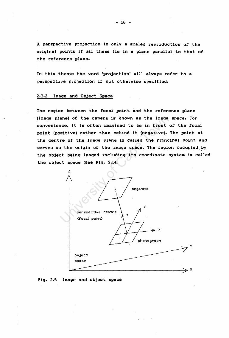
2.3.2 Image and Object Space
The region between the focal point and the reference plane
(image plane) of the camera is known as the image space. For
convenience, it is often imagined to be in front of the focal
point (positive) rather than behind it (negative). The point at
the centre of the image plane is called the principal point and
serves as the origin of the image space. The region occupied,~y
the object being imaged including its coordinate system is called
the object space (see Fig. 2.5).
z
perspective centre
(f'oca.l point)
object
spo.ce
Fig. 2.5 Image and object space
nego.tlve
y
x
photogra.ph y

- 17 -
In this text image space and object space coordinate systems are
labelled with lower (xyz) and upper (XYZ) case letters respectively.
2.3.3 Interior Orientation
In photogrammetry interior orientation refers to the position of
the perspective centre in the image space. It is given by the
position of the principal point (x 0 , y0 ) and the perpendicular
distance from the image plane to the perspective centre (f) (see
Fig. 2.6).
z
perspective centre <U
x
Fig. 2.6 Interior orientation
2.3.4 Exterior Orientation
The exterior orientation of a photograph defines its position and
orientation in the object space (see Fig. 2. 7). Usually, the
position of the perspective centre is given in cartesian
coordinates of the object space (X0 , Y0 , Z0 ). The orientation is
defined by the rotations omega, phi, kappa required about the x,
y, z axes of a cartesian coordinate system parallel to that of
the object, but with its origin at the perspective centre (0), so
that its axes will then be parallel to those of the image space.
Another common system of defining orientation in photogrammetry

- 18 -
is the a (azimuth), t(til t), s(swing) system. However, in this thesis
the omega, phi, kappa system has been used.
z z z z
y rr10.ge plo.ne
x
Fig. 2. 7 Exterior orientation by omega, phi and kappa
The spatial relationship between the object and image space can
be expressed by an orthogonal 3x3 matrix which is a function of
omega, phi and kappa. By convention ~ is the matrix that
transforms the object space into the image space.
[ ~ ] = H * [ ~ ] and
For a derivation of the orientation matrix ~, see Appendix A.
2.3.5 The Collinearity Condi ti on
As mentioned previously, during photogrammetric reconstruction
the perspective centre, the image point and the corresponding
object point must lie on one line. This is the collinear! ty
condition and can be expressed mathematically as
a = k * A (1)
x

- 19 -
where !. . and ~ are vectors as shown in Fig. 2.6 and Fig. 2.8
respectively, and are expressed in the same coordinate system. k
is a scalar.
z L
point on oloject
Fig. 2.8 Collinear! ty con di ti on
Expressing a and A in the x, y, z coordinate system
and
Hence, the equation above becomes 1
[
Ka - x 0 Ya - Yo
-f ] = k *
A =
: ...
This is one form of the collinearity condition which forms the
basis of all procedures in photogrammetry.

- 20 -
2.4 Obtaining the Third Dimension from Two Overlapping
Photographs
Since a photograph is a two-dimensional record of a three
dimensional object, one dimension is lost at the instant of
exposure. Hence, it is generally not possible to recover all the
dimensions from one photogragh. However, if the interior and
exterior orientations of the photograph are known or can be
determined, then the direction of a ray passing from the
perspective centre through the image point can be found from a
single photograph. Where on this ray the corresponding object
point is situated cannot be determined. However, if this object
point is present on two photographs taken from different
exposure stations, then the object point is uniquely defined.
By considering the two ovelapping photographs depicted in Fig. 2.9
the reconstru~tion of an object point can be described. Knowing
the interior and absolute exterior orientations of each
photograph, the direction of the. ray passing through the
projective centre, the image point and the object point is found
by collinear! ty.
J' z projective centre 1
projective centre 2
2
photogro.ph 1
point on object
x
Fig. 2.9 Geometry of two overlapping photographs
- 21 -
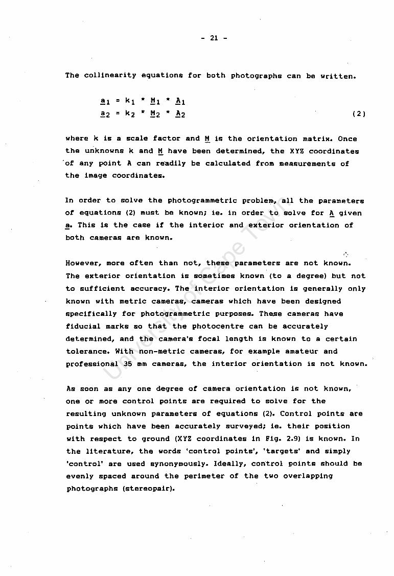
The collinearity equations for both photographs can be written •
.!1 = k 1 * ~1 * !1
.!2 = k2 * H2 * !2 ( 2 )
where k is a scale factor and M is the orientation matrix. Once
the unknowns k and M have been determined, the XYZ coordinates
'of any point A can readily be calculated from measurements of
the image coordinates.
In order to solve the photogrammetric problem, all the parameters
of equations (2) must be known; ie. in order to solve for ~ given
a. This is the case if the interior and exterior orientation of
both cameras are known.
However, more often than not, these parameters are not known.
The exterior orientation is sometimes known (to a degree) but not
to sufficient accuracy. The interior orientation is generally only
known with metric cameras, cameras which have been designed
specifically for photogrammetric purposes. These cameras have
fiducial marks so that the photocentre can be accurately
determined, and the camera's focal length is known to a certain
tolerance. With non-metric cameras, for example amateur and
professional 35 mm cameras, the interior orientation is not known.
As soon as any one degree of camera orientation is not known,
one or more control points are required to solve for the
resulting unknown parameters of equations (2). Control points are
points which have been accurately surveyed; ie. their position
with respect to ground (XYZ coordinates in Fig. 2.9) is known. In
the literature, the words 'control points', 'targets' and simply
'control' are used synonymously. Ideally, control points should be
evenly spaced around the perimeter of the two overlapping
photographs (stereopair).

- 22 -
The number of unknowns determines the number of control points
required. Each control point generates one pair of equations.
Finally, if more control is available than is required redundancy
results. There are various mathematical techniques to solve for
the 'best' solution where this occurs.
2.5 Projective Transformation - Restitution of the Object
As previously stated photogrammetric reconstruction can be done
graphically, numerically, analytically, or by a combination
thereof. Analytical photogrammetry tends to be more accurate
than analogue or semi-analytical methods since it can more
effectively remove systematic errors caused by, for example, lens
distortions. However, from a practical viewpoint a computer i&.
necessary to deal with the large amounts of data and the many
computations generated by analytical photogrammetry.
Restitution of the object consists of precicely surveying ground
control points and measuring their respective coordinates on two
photographs to achieve relative and absolute orientation and, if
necessary, to solve for these separately.
Over the years, various methods in analytical photogrammetry have
evolved. However, conceptually all of them centre around
enforcing condition equations on multiple photographs. The most
commonly used condition equation is the collinearity equation.
The various methods differ mainly in the way the condition
equations are enforced or, how the resulting set of simultaneous
equations are solved.
Outlined below is the projective transformation method (Adams,
1981) which uses the collinear! ty condition. The collinear! ty
equation has been stated in vector form in equation (1) (Section

- 23 -
2.3.6). Equations (3) are merely another form of the collinear! ty
equations for two overlapping phots9raphs and are derived from
the same condition (perspective cent~mage point and object
point must be collinear) as was equation (1). The derivation of
the collinearity equations (3) are given in Appendix 8 and are
repeated here for convenience.
x =
y =
bi1*X + bi2*Y + bi3*Z + bi4
b31*X + b32*Y + bJ3*Z + 1
b21*X + b22*Y + b23*Z + b24
b31*X + bJ2*Y + b33*Z + 1
where x, y are image coordinates (measured from any arbitrary
origin on the photograph), and X, Y, Z are space coordinates of
the corresponding point.
Equation (3) can be rewritten as
bi1X + bi2Y + bi3Z + b14 - b31Xx - b32Yx - b33Zx - x = 0
( 3)
b21X + b22Y + b23Z + b24 - bJ1XY - b32YY - bJ3Zy - y = 0 (4)
Provided there are a sufficient number of control points in a
stereopair, the bij terms (11 unknowns) of equations (4) can be
solved for each photograph. Since two equations can be written
per photograph for each control point, a minimum of six such
points is required - giving one redundancy. However, the following ·
important restrictions must be borne in mind :
1. no more than four control points should be coplanar.
2. no more than three points should be collinear.
Once the b-parameters have been solved for each photograph, it
is simply a matter of backsubsti tution into equations (4) and
measuring the image coordinates of the points of interest on
both plates. Substituting these measured coordinates (x and y)

- 24 -
into equations (4) generates four linear equations in X, Y ,Z (the
coordinates of the object space)-which are easy to solve.
However, equations (3) and (4) are not linear and hence, more than
one 'best' solution is possible. The 'least squares' iterative
approach is popular in photogrammetry and is found in virtually
every book on the subject. Adams (1981), however, argues that in
certain instances a much simpler, faster approach will yield
practical results. A discussion of techniques such as 'least
squares adjustment' is beyond the scope of this thesis and is not
needed to understand the photogrammetric process.
_ . .,._

- 25 -
CHAPTER THREE
3.0 DEVELOPMENT OF A PC-BASED NRTP SYSTEM
With the advent of solid-state cameras, recent developments in
image processing techniques and the ever increasing power of
microprocessors, RTP measurement systems for close-range
applications have become a possibility. The motivation for
developing RTP systems is that photogrammetry with conventional
cameras is:
a. relatively slow,
b. very tedious, and
c. requires special skills.
_.~.
For many applications, especially when studing dynamic scenes, it
is desirable to have an on-line, three-dimensional measuring
system. This is the ultimate goal. Real-time strictly speaking
implies that the system's response time must be within one video
cycle (ie. < 1/25 or 1/30 second). To the author's knowledge truely
real-time, 3D mensuration systems did not exist at the time of
writing. However, a number of NRTP systems have already been
developed. A NRT process, although longer than a video cycle
practically provides immediate results. For many applications a
NRT system presents a very big improvement on the conventional
photogrammetric process.
RTP and NRTP camera systems already developed (Wong and Ho 1986,
Haggren 1986, El Hakim 1986) typically rely on expensive mini- or
mainframe type computers. However, decreasing prices and
increasing processing power of PCs will change this in the
future.

- 26 -
The stages in design of a RTP process are:
1. Image capture.
2. Target design ie. design of a suitable reference frame and
targets to provide ground control.
3. Design of algorithms for target detecting, target centre
extraction and target matching.
4. Design of algorithms for image matching ie. algorithms
which will measure a number of object points on two or
more images and then perform object point matching.
5. Design and development of photogrammetric software, more
specifically, software which:
a) receives as input pairs of matched image coordinates of
the targets.
b) solves for camera orientation (implicitly or explicitly
depending on the photogrammetric method used).
c) uses the constants determined above to transform pairs
of matched image coordinates of points into 3D space
coordinates.
6. Design and development of application software to make
the system user friendly. The various software
components that are developed and the functions
performed by the bought in soft- and hardware must be
integrated.
The next section describes the hardware and the software that
has already been developed for a low-cost, PC-based NRTP system -
PHOENICS (Photogrammetric Engineering and !ndustrial £amera
_§ystem). Future extensions to PHOENICS are also discussed.
PHOENICS is being developed by UCT's Department of Surveying and
has produced some promising results in its initial stages.
Although the long term aim is to produce a real-time system,
speed is of lesser importance when configuring hardware and
developing software for a prototype system. The dimension of
real-time or near-real-time will be added later.

- 27 -
Hardware Configuration of PHOENICS
The present hardware configuration of PHOENICS is shown in Fig.
3.1 and Fig. 3.2 below.
PHOENICS
, .. CCD I I
Siemens K211
5 1
00 x 582 7x11 µm pixels
I " CCD I
Matrox PIP-512
A-D Converter Framegrabber/store
Matrox PIP-1024
A-D Converter Framegrabber/store
~ ... 11111111111111 11111111111111111111111111 ll111111n\
Tektronics Image Printer
r "I I System } '-Control..., Porollon i.-
1:::::::::::::::::::::::t Porollel - liitif:i\~ffiI::::=: :::::.'£1111.mi.l.Wl.i.f ~ Pro-IBM PS/2 M3C cessor
- I Image I mag~
Display - - Display
0 0 0 0
Phillips RGB Monitors
Fig. 3.1 Schematic of PHOENICS hardware configuration
The host computer is an IBM-Personal System/2 Hodel 30 and has a
high resolution monochrome screen. Images can be displayed in
formats of 640x400 with 16 grey shades or 320x200 with 64 grey
shades on the PC screen, or complete images may be displayed on
the two RGB monitors with 256 shades of grey. Motivations for
the choice of this PC are given by Parkyn and Ruther (1988).


- 29 -
The system uses two Siemens K211 monochrome solid state charge
coupled device (CCD) cameras to perform image capture. The
physical size of the sensor is approximately 9 mm x 7 mm and
consits of 500x582 pixels. The frame grabbing time is 1/25 second.
A pixel is the smallest unit area over which the average light
intensity is measured.
Al though CCD's are also termed 'digital' cameras, their output is ·
in fact a continious analogue amplitude modulated signal. An
analogue to digital (A/D) converter then produces an array of
intensity levels representing the image. CCD technology has made
possible the, development of RTP systems. Some of the
fundamentals of the technology are given in chapter 4.
As mentioned earlier, the CCD cameras provide 25 frames per
second as an analogue signal •. Each video image is converted~~ an
array of 8-bi t pixels (representing 256 shades of grey) and then
passed through look up tables (LUT), in which the grey values are
transformed in a predetermined manner. The image can either be
stored on disk or it can be converted back to an analogue signal
and displayed. To acieve this in 1/25 second for 0,25 million bytes
in the case of PHOENICS, additional hardware known as
framegrabbers or video digitizers must be added to the PC. Often
such video digitisers include some processing software and are
then called image processing (IP) boards. Typical operations
possible with an IP board are edge enhancement, noise removal,
thresholding (ie. producing black and white images from 'grey'
images), inverting images, changing the grey value of any pixel
etc.
Phoenics has two IP boards, the HATROX PIP-512 and PIP-1024,
allowing simultaneous stereo imaging. The boards fit directly into
the PC and digitise the analogue signals from the two cameras
into 512x512 pixels with 256 shades of· grey. This means that 15%
of the camera image is lost and the original pixels are

- 30 -
transformed in size. However, Parkyn and RUther (1988) state that
this can be dealt with in the photogrammetric solution.
Each board has a 256 kbyte buff er, enough to store one image.
Once in the board-buffer, images may be stored in memory, or on ~
hard or floppy disk for later processing.
At present, parallel processors are being added to PHOENICS to
decrease processing time. Parallel processing allows operations
which must be performed on a number of pixel arrays to be done
simultaneously.
Images which are generated with PHOENICS can be printed using
the Tectronics image printer.
Software developed and used with PHOENICS includes automati~.
target detection and calculation of object coordinates of
targeted object points using projective tranformation. For
automatic target detection a binary image is first created with
the MATROX IP. The pixels of the original image are mapped to
one of two chosen values depending on whether their grey values
are above or below a specified threshold value. For successful
thresholding, targets should appear considerably lighter or darker
than the backgound. Once targets are found, their centres are
determined using a weighted mean technique (Wong and Ho, 1986) on
the original image.
Experimentation with various target designs for control points
revealed that the fallowing design produced the best results (see
Fig. 3.3).

- 31 -
front view sectlona.l side view
cylinder painted matt
black on the inside
and white on the outside
Fig. 3.3 Control point target design for PHOENICS
First results of automatic target detection and subsequent
projective transformation of targeted points have revealed
accuracies of 0,5 mm in X and Y, and 1 mm in Z for a camera to
object distance of 1,7 m ie. 1:3400 to 1:1700.
=.,.·
Currently work is continuing on introducing parallel processing
to PHOENICS, camera calibration and testing, and the development
of image matching algorithms. The latter is the subject of a
later chapter.
As was previously mentioned, many RTP and NRTP systems are
dedicated systems, as truly general systems become extremely
complex. The way in which PHOENICS hopes to address this, is by
producing software modules which are efficient for specific
applications, and allowing the operator to choose the best
combination of these modules for a particular application.

- 32 -
CHAPTER FOUR
4.0 IMAGE AQUISITION WITH CCD CAMERAS
This chapter is intended to serve as an introduction to the
technology of self-scanning solid state cameras and the older
vidicon cameras. At the end of the chapter the two types of
cameras are compared.
Advancements in microelectronics and semiconductor technology
over the past 15 years have opened up new avenues for the data
aquisition phase of the photogrammetric process. Photographic
cameras can be replaced by digital ones and combined with fast
data flow to a computer for further image processing. The advent
of digital cameras has made possible the development of RTP : ....
systems.
There are two main reasons why RTP is not possible with film
based cameras. Firstly, there is the lead time for developing the
film, and secondly, these negatives must first be digitised to
perform tasks such as automatic target detection and positioning,
and automatic image matching.
Apart from this, it is interesting to note some distinctive
characteristics of digital (or solid state) cameras when
comparing them with film-based cameras (Gruen, 1987).
Digital cameras have:
- a very small imaging area (< 100 mm2) and hence a small image
scale
- limited resolution; presently photogrammetric cameras have a
better spatial resolution than digital cameras
- fixed exposure time; the integration time can not be
altered
- an extremely stable image plane
- possible electronic noise.

- 33 -
Of these characteristics, the extremely stable image plane is the
only one in favour of digital cameras.
4.1 The Vidicon Camera Tube
The vidicon tube is the basic principle on which a TV camera
operates. The vidicon is a cylindrical glass envelope containing
an electron gun at one end and a photoconductive target covered
by a thin, positively-charged metal coating at the other (Fig.
4.1). A lens system produces an image of the scene on the
photoconductive target.
electron gun (-ve>
electron be QM
enla.rged view
of ta.rget
Fig. 4.1 Vidicon Camera tube
lens
electron be QM
photoconductlve tQr et
light
Met QI optic QI COQ ting IMQQe (+ve>
oloJect

- 34 -
The electron beam scans across the back of the target and
deposits electrons on it. When light strikes the photoconductive
target the electrons flow through it to the positively charged
metal coating thereby locally depleting the deposited electron~
Thus, an optical image formed on the front of the target will
result in an identical electron image on the back of the target.
When the beam subsequently scans the target and replaces
electrons in the depleted regions a current flows. This current
is proporional to the electrons required to restore the original
charge which in turn is dependent on the light intensity at
that point. While the electron beam continuously scans the image,
the changing current flow produces the video signal of the
vidicon. Control over the electron beam is exercised by an
electric field surrounding the tube.
The European video standards (PAL for colour and CCIR for black
and white) define 625 lines at a frequency of 25 Hz. In actual
fact, the video image consists of two half images of alterate
lines scanned at 50 Hz which are superimposed. This interleaving
of two image 'fields' is known as the interlace principle. As a
number of lines are required for syncronisation and other
purposes only 575 lines remain for the image (Schild, 1988). An
image thus consists of a number of lines each of which is an
amplitude modulated signal. This is the big difference between a
CCD and the vidicon tube - the image is only discretised in the
vertical direction. In order to provide a basis for comparison of
the two the following approach can be adopted: Since
theoretically the smallest vertical resolution is one line we
can expect/assume the same resolution horizontally ie. a square
picture cell as the smallest image element. From the base to
height ratio (4:3) of a TV screen this would mean that there are
575x764 (= 440 000) picture cells in a video image.
A frame rate of 25 Hz of an image with 440 000 picture cells
translates to a pixel scanning frequency of 11 MHz. To increase

- 35 -
the resolution, a larger image is required which in turn requires
a higher scanning frequency in order to comply with the video
standard. Until recently larger images were riot produced because
of the difficulty to keep within the video standard requiring 25
frames per second. However, Japanese research dating back to 1970
has now produced High Definition Video (HDTV) with a resolution
of approximately 1300x1000. At a frame rate of 25 Ha this
translates to a pixel frequency of about 32 HHz. At present such
frequencies can only be achieved with tube cameras (Gruen, 1987).
4.2 Solid State Sensors
Solid-state sensors use semi-conductors to transform light into
an electrical signal. Unlike vidicon tubes, solid-state sensors do
not have a scanning electron beam neither do they have any
other moving parts. In the literature, the terms 'CCD' and 'so~id
state cameras' are often used synonymously. Strictly speaking,
however, this is incorrect since a CCD is only one class of solid
state camera making use of a particular technology. Furthermore,
solid state cameras are often termed 'digital cameras'. Again, this
is not necessarily correct. The output of these devices is more
often an amplitude modulated, analogue signal and not a digital
one. The analogue signal is digitised for computer processing, but
with a separate technology.
· Basic theory of semiconductors
The characteristic of intrinsic semiconductors, those that are
not doped or pure, is that all their outer electrons are resident
in their lowest possible energy level known as the valence band.
By supplying external energy a few electrons will be able to
leave the valence band and enter the conduction band, a much
higher energy level. This would leave a hole in the valence band
and the net positive charge of the atom will attract another
electron. In this way, holes and electrons can move through the
lattice (ie. the conductivity is increased). The extent to which

- 36 -
this phenomena occurs can be controlled by 'doping' the
semiconductor with an element having fewer or more valence
electrons than itself (ie. creating more holes or free electrons).
Every time a hole and a free electron combine energy is
liberated. This process can also be reversed by supplying energy
in the form of light to produce an electron hole pair.
The photodetector
A photodetector changes light (energy) into electrical energy. If
a.potential difference is applied accross a doped semiconductor,
the current that will flow is proportional to· the amount of
light failing onto it.
Through integrated circuit and recent semiconductor technology
such sensors can now be built extremely small (to a few square
micrometres) and positioned accurately to fractions of microns in
a matrix. What remains to be done in order to record an image is
to collect all the electrical signals from each sensor and process
them. Solid state cameras can be classified according to the type
of signal they have as output. The three categories are:
- CCD (fharge foupled gevice)
- CID (fharge !njected gevice)
- Photodiodes
RTP systems normally use CCD cameras.
4.3 CCD Cameras
A CCD camera has photodetectors with a HOS structure (Hetal
Oxide-Semiconductor). It consists of a doped semiconductor, an
insulator (glass) and a metal electrode (Fig. 4.2). A large number
(between 200 and 2000) of these photodetectors are arranged next
to one another to form a sensor row.

- 37 -
I I 1
rrie to.l electrode
_...__ insulo. tor ++++++++++++++++++
I ------------------ I ...._~~~~~~~~~~~.i.--1~~~
TTTT light
Fig. 4.2 CCD HOS structure
doped serriiconductor
Applying a positive potential to the metal electrode, called a
, gate, will lead to a negative charge build-up on the other side
of the insulator. The extent of this charge build-up depends on
the amount of light falling on th~ detector. The more light
there is, the more free electrons there are, the larger the
charge. The charege build-up is also a function of the number of
free electron-hole pairs in the semiconductor (this depends on
the extent of 'doping' and does not vary with time).
The way in which the accumulated charge of a whole row of
adjacent sensors is transported depends on whether the device is
a 2-, 3- or 4-phase CCD (D~hler, 1986). In each case, however,
charges are transferred along lines parallel to the row of
sensors.
If a number of sensor rows are placed next to each other they
make up what is known as the sensor array. It is the shiny area
(less than 100mm2) which can be seen in the image plane of a CCO.

- 38 -
4.3.1 Interline vs Frame Transfer
CCDs can be categorized according to how the charge transfer of
the sensor array takes place. There are two methods by which
this is done; interline transfer or frame transfer.
Interline transfer
The image area of the interline design consists of alternate
columns of photosensitive sensors and opaque shift registers (Fig.
4.3).
tra.nsfer ga.te
light sensitive pixels
readout register
Fig. 4.3 Interline charge transfer
vertlca.l CCDtra.nsport registers
output
During the integration time ('exposure' time) charge is
accumulated at the photosensors and is then passed to the
adjacent shift registers for storage. From there the charges are
shifted vertically to the horizontal line readout register on the
next integration cycle. In this way an image, in the form of
light induced charges, is sent out of the camera pixel by pixel
onto one single video line. Since the number of imaging columns
is the same as the number of shielded readout registers, only
half of the chip area is photosensitive.

- 39 -
Frame transfer
In the frame transfer type image plane CCD cells are practically
in contact horizontally and vertically (Fig. 4.4).
vertlco.l CCDreg1sters o.na CCDtro.nport cho.nnels
CCD cells
v
<~ ~
I
sepo.ro.tors
/ "-.
I I
reo.aout register
Fig. 4.4 Frame charge transfer
-
-
p 0.
~
storo.ge o.reo.
hotosens1t1ve reo.
output
Half of the chip area is optically sensitive and accumulates
charges during the integration time. Subsequently, the charges
are transfered in parallel to the storage area which is shielded
from light. The stored charges are read out through a horizontal
shift register in the following integration period.
The advantage that interline has over frame transfer is the
absence of smearing. Smearing occurs in frame transfer because
exposure of the photosensitive areas continues during charge
transfer. As a result, a charge being transfered past a very
bright spot tends to pick up some additional charge. This appears
as a fine, faint vertical line beginning at a bright spot on the
display. The more complicated architecture of the interline
concept eliminates smearing.

- 40 -
An important factor to consider when imaging dynamic scenes is
the integration time of the device. The integration time for a
frame transfer sensor is half that of an interline sensor and
thus the former will record fast movements more clearly (Schild,
1988).
The main cause for. differences between the two concepts is that
with interline pixels are separated. This means that for a fixed
total chip area and number of pixels, the lightsensitive areas
are equal, merely distributed differently. However, since the
light sensitive pixels in an interline design would be distributed
over an area twice the size as that of the frame transfer
design, the latter will have a better resolution. If, on the
other hand the same number of pixels cover the same area for
both designs, their resolution will be equal yet the interline
sensor would only have half the light sensitivity. These
observations have made frame transfer CCDs more popular with
photogrammetrists (Real, 1986).
A phenomenon that an interline sensor can suffer is Moire-effect.
This only occurs when imaging objects of very fine structure.
Instead of showing an average intensity over an area, the image
displayed has alternating light and dark bands.
One problem with all solid state cameras except CIDS (Real, 1986)
is blooming. Blooming is known as that effect which causes a very
bright spot in the object space to appear larger in the image
than it really is. It is caused by the creation of excessive
charge and subsequent overflowing of charge to adjacent pixels.
Automatic aperture setting can not solve this problem as it
responds to the average illumination of the whole scene.
Fortunately,- new technology will ensure that blooming will soon
be a thing of the past (Dahler, 1986).
- 41 -
4.3.2 CCD Performance Features
Commercially available CCDs have area arrays ranging from 128x128
to 600x600 pixels usually covering less than
100 mm2. The size of an individual pixel ranges from 60x60
micrometres down to 10x16 micrometres. Pixel intensity is usually
converted to an 8-bit byte. This represents 256 grey scales. An
exeption is the high resolution Kodak Hegaplus CCD which has an
area of approximately 9x7 mm containing 1320x1035 pixels.
Two current limitations of CCDs are their very small imaging
areas and spatial resolution. Unfortunately, these limitations can
not simply be overcome by manufacturing larger format CCD arrays.
These would require improvements to the present charge transfer
technology. They would also require hardware capable of processing
the vast amounts of data that will be generated within one .
video cycle. Other approaches are mosaicked-arrays (Gruen, 1987)
and zig-zag arrays (Hirschberg, 1985).
As mentioned earlier, the charge generated in a pixel is sent out
of the camera in analogue form and is then digitised. However,
seldom is the number of pixels in the image plane the same as
those produced by the analogue to didi tal (A/D) converter: eg. in
the case of PHOENICS a 568x468 image array is transformed to a
512x512 array by the A/D converter. The question thus arises of
what happens geometrically to these pixels and what the effect
is on camera resolution. This problem is specific to the
particular hardware configuration and must be investigated
wherever measurements on the image are to be made.
CCDs used in photogrammetric applications are usually of the
black and white type. Colour CCDs do however exist. In these
devices incomming light is split up into three colours (red, blue,
green - RBG) with a lens system, and their intensities are
recorded by three different phqtosensitive arrays. They are

- 42 -
processed separately and then displayed on an RBG monitor. The
obvious disadvantage is that spatial resolution decreases since
an object space represented by one pixel in a black and white
image, now requires three or sometimes even four pixels depending
on the CCD design.
4.4 CCD vs Vidicon Tube Cameras
Although both solid state and vidicon tube cameras may be used
for real-time photogrammetric applications, vidicon cameras are
not expected to be used for this purpose in the future because
they suffer from large geometric distortions. Real-time systems
currently being developed (Haggren, 1986; Gruen, 1986; Wong, 1986)
largely use CCD cameras. CCDs are pref erred over Vidicons for the
following reasons:
- high geometric fidelity of array picture elements in sp~ce
and time
- small, lightweight and rugged
- low power consumption
- high dynamic range
- maintenance free
- no damage through overlighting
- low cost
Factors in favour of Vidicons are:
- better operation at lower light level
- higher resolution and less Moire
- faster image capture
The overriding factor responsible for photogrammetrists turning
to CCD cameras for real-time applications is their metric
stability.
The higher resolution of Vidicon tubes applies to comercially
available cameras. It was pointed out earlier that the average TV

- 43 -
has an equivilent ,of approximately 440 000 pixels whereas for an
average CCD the figure is below 350 000. Especially with the
development of comercial HDTV with around 1000 lines (equivalent . to 1,3 million pixels) the better resolution of electron tube
imagers is emphasized. Nevertheless, CCD resolution is good enough
for many photogrammetric applications.
The limiting factor preventing larger photosensitive chips with
more pixels is charge transfer efficiency (CTE). The CTE is the
efficiency with which a charge can be transferred from one
photocell to the next. It depends on the available charge
transfer time which in turn is dictated by the frame rate. At
- present CTEs of 99,9999 % are being achieved with comercial CCDs
that comply with the video standards (frame rate of 25/second).
The effect of increasing array sizes, is a decrease in charge
transfer time since more charges must be transferred in the ~ame
time. Since the time allowed for charge transfer is less, the CTE
will also decrease. This results in a generally poorer image being
displayed. However, larger format CCDs with higher resolution are
possible as the frequency of charge transfer in todays cameras is
only between 1% and 10% of the theoretically possible value.

- 44 -
CHAPTER FIVE
5.0 A REVIEW OF NRTP SYSTEMS WITH REFERENCE TO THE IMAGE
HATCHING TECHNIQUES USED
One of the most difficult operations in photogrammetry to
automate is image matching. As explained in chapter 2, after
having solved for camera orientation using control points it is
necessary to identify a sufficient number of corresponding object
points on the two images that will enable reconstruction of the
surface from these points.
Keefe and Riley (1986) state that this becomes particularly
difficult on relatively featureless surfaces like a human face.
According to Wong (1987) present algorithms for digital image .
correlation can not match the capability of an experienced human
operator. This applies in particular to close-range applications
because of the large difference in perspective from one camera
position to another. El-Hakim (198~ giv~s some of the factors
which complicate automatic matching. Some patches may appear
with different brightness in the two images. For surfaces with a
certain shape or ·texture, where the light intensity is the same
for all surface points or follows a periodic pattern, there will
be no unique solution. Further, clarity and contrast of special
features such as edges or targeted points varies from one scene
to the next, because pixel grey values are affected by surface
material, intensity and angle of illumination, camera location and
orientation, and atmospheric conditions. It is very difficult to
predict the influence these parameteres will have. Some of these
problems could even be of great obstacle to a human operator.
A number of techniques for solving the matching problem have
evolved over the years. Host of these methods were established
whilst developing a NRTP or RTP system. As a result they are
usually part of a dedicated system and hence rely on specific
equipment and/or a controlled enviromental condition. Presently,

- 45 -
matching is solved using stereopairs consisting of parallel or
convergent digital images and algorithms which find corresponding
points. In some cases one of the two images of the stereopair is
replaced by a structured light projector with known perspective
geometry to simplify the matching process.
The following sections briefly describe some NRT systems which
employ automatic and semiautomatic image matching. Digital image
correlation, a general image matching algorithm, is discussed at
the end of this chapte~
5.1 Isis Scanner
In an effort to gain some guantitive record of the shape of a
human back in order to assess various spinal disorders, Turner
Smi th and Harris (1986) developed the Isis Scanner. It consist~ of
a projector producing a plane of light and a vidicon camera (see
Fig. 5.1).
ca.Mera. IMa.ge
projector
Fig. S.1 Principle of operation of the Isis Scanner

- 46 -
The position and orientation of the camera with respect to the
projector is known and fixed. This assembly, camera and projector,
can be rotated so as to move the plane of light across the
surface. As the assembly rotates, camera images are stored at
known degrees of rotation. The line of light on the surf ace is
seen by the camera as a profile. Once the scan is complete the
three-dimensional coordinates along the profile lines can be
determined by considering the geometry of the system.
The RMS errors of relative measurements made through a volume of
350x7soxJ100 mm were reported as ±1.1 mm in X, ±1.S in Y and ±1. 7
in z. These RHS values translate to accuracies of approximately
1:300, 1:500 and 1:60 in the X, Y and Z directions.
The Isis Scanner is similar to the TopoScanner used by Berelo~itz
(1986) which also solves the matching problem by capturing a large
number of images which contain a small amount of information.
Since the pattern is simple, there is no ambiguity when
calculating coordinates. However, the accuracies achieved with
the Isis Scanner are not accepable for the applications intended
here.
5.2 Mapvision
Hapvision is a commercially available, RTP machine vision system
developed at the Technical Research Centre of Finland_(Haggren,
1986). Mapvision uses up to four CCD cameras and an 'especially
developed photogrammetric microprocessor'. In order to extract 30
information from a surface, individual points on the object must
either be targeted or pointed at with a laser beam. In a way,
this approach is similar to the Isis Scanner system of simplifying
the matching problem by processing a number of images containing
a small amount of information about the surface. Since only one
object point appears in each set of images, matching is easy.

- 47 -
Developing algorithms to recognise a well targeted point or spot
of light on the object is a relatively simple matter.
To measure a surface with Hapvision necessitates targeting or
pointing to a large number of points on the object. Haggren (1986)
reports a relative accuracy of 1:5000 which means that a point on
the object 5 meters from the camera is measured with an accuracy
of 1 mm. In order to measure with this accuracy, assumed to be
under ideal conditions, each point requires one second of
processing time.
5.3 A RTP System for Object Measurement at the National
Research Council of Canada
A system for automatic measurement of 30 coordinates of targeted
points has been developed at the National Research Council ~!
Canada, Ottawa (El-Hakim, 1986 and 1985). This RTP system uses a
program which combines image processing, pattern recognition and
photogrammetric algorithms to automatically map targeted points.
These points take the form of filled circles or grid intersections
on a highly contrasting background. Points are recognised and
accepted as targets by comparing their geometric characteristics
with a set of parameters of an ideal target. No information is
given by the authors as to how a grid point is recognised or how
its centre is determined.
Once the position of control and targeted object points in both
images has been determined, matching commences. The a priori I
knowledge about the number and arrangement of control points is
used to validate and identify the control points in each image.
El-Hakim (1986) suggests having control points with different
shapes to uniquely define them as an alternative for easy
matching.
Subsequently, epipolar geometry is used to match targeted object
points in the two images. For each targeted point appearing in

- 48 -
' the one image, the corresponding epipolar line in the other image
is calculated. The point in ·the second image which best satisfies
this line is the matching ~oint. For an explanation of how
epipolar geometry can be used as a matching technique, see
Appendix c.
Highly contrasting targeted object points were measured with an
accuracy of 0.15 mm. Since the distance over which the results
presented were obtained is not given, the resolution of the
system cannot be quoted here. However, if the assumption is made
that the object's image covered the entire active area of the
CCD cameras which were used (illustrations in the article suggest
that this was the case), then it can be said that a relative
accuracy of approximately 1:2000 was achieved.
5.4 A Close-Range Mapping System at the University of Illinois
A close-range mapping system using solid-state cameras developed
by Wong and Ho (1986) is described below. The object, a toy moose,
was imaged at a distance of 0.9 m. First, the coordinates of the
control ·points (6 mm black dots on a white background) on the
digital image were located as follows. Manual indication of the
approximate control point position was followed by automatic
thresholding of a window containing the control point. The
weighted mean technigue was used to determine the centre, and
various shape, size and location criteria are applied to check the
validity of the target. The position of these control points was
determined with an error of ±0.2 mm in X and 'i and ±0.4 mm in z. This is equivalent to a relative accuracy of- approximateley
1:2000.
Wong and Ho (1986) use a correlation function to match a search
array in the second image with the target array of the first
image. These arrays are typically 7x7 pixels. To guide the search
the position of pairs of epipolar lines are computed. The position

- 49 -
of the probable matchpoint is estimated using sets of previously
determined matchpoints and the search is performed along the
direction of an epipolar line (Fig. 5.2).
left photo conjugQte MQtch po~ts right photo
conjugQte
eplpolQr lines
' eplpolQr
"--~/ ~~I
seQrch ~ ·~ direction
Fig. 5.2 Image correlation along epipolar lines
line
--- ...... r--.
Tests done with a number of one and two dimensional target array
sizes revealed that although larger arrays gave consistently
higher success rates of finding a matchpoint, the position
accuracy did not improve in the same manner. A 1x9, 1x5, 5x5, and
an 11x11 array produced similar accuracies, but CPU time increased
markedly for arrays larger than 5x5.

- 50 -
5.S Robot Vision at the National Research Council of Canada
El Hakim (1985) presents a visio~ system based on a light strip
sensing technique which in principle is similar to the Isis
Scanner system (Turner-Smith and Harris, 1986) described earlier.
projector pla.ne
Fig. 5.3 Optical beam deflection assembly
pla.ne of
------ ll gh t
a.rgon la.ser
~ "'.
An optical beam deflection assembly (Fig. 5.3) produces a single
line of light on the object from an argon laser. The object is
scanned with the plane of light (1 second for simple objects) and
at predetermined intervals the assembly accurately determines the
line position on the projector plane. A control unit syncronizes
camera (CCD) activation at the same intervals. Image processing
removes noise from the images, and then a number of points on
each line are extracted. Accurate x and y coordinates of these
line points are determined using thinning techniques (Kreis et al,
1982 in El Hakim, 1985).
Before measuring an object, the camera and light source are
calibrated. This is done via a test object with a series of
precisely measured control points. Briefly, the calibration process
proceeds as follows. First, the unknown orientation parameters of
two cameras are determined using the control points in the usual
- 51 -
way. For the light source the interior orientation is known and
fixed and the parameters of exterior orientation are determined
as follows. The light plane is projected onto the object and the
image coordinates of a number of object points on the light
strip are used to determine their true XYZ coordinates. This is
repeated for different line positions on the projector plane. In
a sense, the two cameras are used to generate a set of control
points with which the light source is calibrated. From the
collinear! ty equations for the light projector, its orientation
parameters can be determined. The light source-camera system is
now calibrated.
Knowing all the orientation parameters, the true object
coordinates of any object point can be derived from the x, y
image coordinates and the position of the light strip (one
coordinate on the reference plane).
The system was used to recognize, in real time, shapes and
positions of simple objects such as cylinders for robot
manipulation.
No indication of system accuracy is given.
5.6 Rasterstereography
Rasterstereography is quite similar to conventional
stereophotography except that one of the two cameras is replaced
by a projector with a raster diapositive. This approach, of
projec.ting structured light. onto the object., is essentially the
same as that. presented by Turner-Smith and Harris (1986) and El
Hakim (1985) described earlier. The only significant. difference is
that. in rasterstereography a pat.tern is projected over the
entire surf ace and only one image of the camera is processed.
The pat.tern projected is either a grid, a series of crosses, or a
set of parallel liries (Fig. 5.4).

- 52 -
projector ca.Mera.
Fig. 5.4 Cross- and line rasterstereography
In cross-rasterstereography only raster intersections are
evaluated for the reconstruction of surface points. In order to
perform photogrammetric reconstruction of these points the
column and row numbers of a raster intersection must be known
(defining the 'image point' in the projection plane) as well as
the x, y coordinate in the camera image. Although this appears to
be relatively simple to do, it does not lend itself to automatic
image processing (Frobin and Hierholzer, 1981).
Line-rasterstereography, however, is suitable for image processing.
Kn.owing the raster line number and the position of any arbitrary
point along this line leads to a unique solution of the XYZ
coordinates of the object point. However, since there is one
degree of redundancy in a cross-raster image and none in a line
raster image, the former will enable more accurate results.
Algorithms for automatically analysing line rasters have been
developed and tested (Frobin and Hierholzer, 1983a, 1983b).
As with any photogrammetric system, control is required to solve
for unknown.orientation parameters. Methods of extracting

- 53 -
control points from rasterstereographic images are given by
Frobin and Hierholzer (1981, 1982, 1983a, 1985).
Frobin and Hierholzer (1983b) report processing times of
30-40 minutes for complete evaluation of a rasterstereograph of a
human back. No quantitive information of system performance is
presented.
5.7 A system for Capturing Facial Surface Information at the
University of Minesota
Keefe anf Riley (1986) have developed a system that semi
automatically generates 30 surface information of a human face.
The system s~tup is a conventional one with two cameras (not
digital) and a control frame to solve for camera orientation.
:"'.
Automatic image matching has been eff ec~ as follows. A single
line ~f dots is projected onto the human face by passing a single
low-power laser beam through a collimator, a cylindrical lens and
an opaque barrier containing small holes. This produces an 80 dot,
140 mm long line segment in the object space. The laser line of
dots is projected onto the subject and photographed. To capture
the entire surface multiple stereopairs with the beam in
different positions are necessary. After the film has been
developed it is digitised and the dot patterns for each
stereopair are matched. This is done by determining the position
of the dots closest to the control frame and comparing the
spacing between adjacent data spots. Image processing algorithms
determine whether any data points are hidden in one view, and if
that is the case, will discard their corresponding points in the
other view.
\
Photgrammetric algorithms are then used to determine the XYZ
coordinates of the dots which were matched in the various
stereopairs. From these XYZ coordinates, the surface is
- 54 -
reconstructed. Finally, the system has computer graphics software
which enables the user to view the reconstructed surf ace.
5.8 Digital Image Correlation
Digital image correlation is an approach to image matching in
which corresponding pixel arrays of overlapping digital images are
searched for. Only once a matching pair of arrays has been found,
are the respective image coordinates of the match points
determined. This is different to the methods discussed previously
in which the precise position of a targeted point or distinct
pattern is first determined in each image.
The method frequently used to find the approximate position of
the array to be matched in another image is the use of epipolar
geometry (Wong and Ho, 1986). Up until recently the most commonly ~ "'.
used algorithm to match two image windows tries to maximise the
cross-correlation coefficient of the two arrays by moving one
relative to the other in a systematic trial and error procedure.
However, a number of fundamental aspects that crosscorrelation
cannot address, have caused a slow-down in the development of
operational automated correlation systems (Gruen, 1985). Conjugate
images may differ condsiderably from each other due to a number
of reasons. Some of these are differences in height, positional
and attitude differences of cameras which cause geometrical
distortions, and illumination and reflectance conditions which
distort images radiometrically. Furthermore, noise from electrical
components may influence image appearance. Crosscorrelation only
works well "if the patches to be matched contain enough signal
without too much high frequency content and if geometrical and
radiometric distortions are kept to a minimum" (Gruen, 1985).
As these phenomena are often present in typical images, efforts
in recent years have been directed at developing alternate
correlation algorithms. Ackermann (1984) adopted an approach in

- 55 -
which an array pair with minimum grey value differences qualifies
for the optimum match. An iterative least squares solution is
used to determine parameters to rectify geometric and radiometric
distortions in the process of array matching. Another approach,
also making use of the least squares technique, is presented by
Gruen (1985).
5.9 Conclusions
In the 30 vision systems described above, the different.
approaches to solving the matching problem can be summarized as
follows:
1. One approach simplifies matching by evaluating a number of
stereo image pairs taken from the same camera position,
each of which contains information about part of the
object. As image scanning takes a few seconds, this method
can only be applied to perfectly static scenes. Expensive,
specialised equipment is required.
2. One of the cameras is replaced with a ~ctured light
projector with known perspective geometry. Expensive,
specialised equipment is required.
3. Epipolar geometry.
The methods of image matching which fall into categories 1 and 2
above require expensive hardware which is not part of PHOENICS.

- 56 -
CHAPTER SIX
6.0 DEVELOPING AN AUTOMATIC IMAGE MATCHING ALGORITHM
After reviewing a number of image matching algorithms used in
existing and developing photogrammetric systems it was concluded
not to adopt any of these approaches (chapter S), but rather to '
develop one in-house. After having designed a suitable algorithm
it had to be programmed and tested on real image data.
One of the principal objectives of the thesis was to obtain a
number of spotheights of the object surface to be measured, or
in photogrammetric terms, XYZ coordinates in the object space. As
it was intended to use the XYZ values as input data for the
millin'g program developed by Back (1988), the measured object
points had to be in an approximately grid-like structure.
6.1 Problem formulation
The need for a general, automatic image matching algorithm is the
long term requirement of PHOENICS. To start with it was decided
that a less general algorithm had to be developed. The problem
definition was as follows.
6.1.1 Problem Statement
Develop, program and test an algorithm to be used with PHOENICS
for matching conjugate object points which are approximately in a
grid-like pat tern.
6.1.2 Require men ts
The problem specific requirements were:
(i) The matching algorithm had to have an accuracy of
better than O.S pixels (this was considered sufficient
for the prototype).

- 57 -
(ii) The program input be resticted to the image name and
the starting point of the image search.
(iii) The program output be a set of matched image coordinates
(ie. x and y coordinates in the left and right images).
(iv) The measured points on the object to be in a grid-like
pat tern suitable for the milling program.
(v) Physical contact with the object for targeting purposes
not be allowed ie. the measuring technique to be "non
contact".
6.1.3 Constraints
(i) The programmed algorithm be be executable on an IBM
microcomputer (part of the PHOENICS hardware) with 640
kB RAM; apart from memory limitation, this constrains
the number of instructions that can be programmed as
the program should run to completion within a reasonabe
time.
6.1.4 Criteria
(i) As the image processing card only supports the Microsoft
(MS) 'C' and MS-Fortra'n computer languages, no other
computer languages allow direct access to the IP. With
MS-'C' and MS-Fortran the PIP card's soft- and hardware
routines and libraries may be directly used in a program.
This has speed and convenience as an advantage. TRUE
BASIC is the next pref erred choice.
(ii) Fast program execution.
(iii) Efficient algorithms and computer programs.
(iv) Well structured programs so they can be understood by
subsequent researchers.
(v) User-friendly programs.
. r Before some of the concepts which were considered are descibed,
some background is given on the images to be analysed.

- 58 -
With the PIP image proccessing software an image is displayed on
a TV monitor as a 512x512 array of pixels each having an
intensity level between 0 (black) and 255 (white) ie. there are 256
'shades of grey' or 'grey levels'. An example of such an image is
shown in Fig. 6.1 and the grey levels of a portion of it are
shown in Fig. 6.2. These images will henceforth be referred to as
a 'grey' images.

Fig. 6.1 Example of a grey image
U'1 IO

- 60 -
158 155 153 156 157 157 156 1C9 123 92 92 123 151 160 159 159 166 166 16• 152 151 151 152 158 161 153 139 113 87 89 116 142 155 160 163 16 7 165 163 15• 153 153 155 155 15, 150 137 111 86 86 112 138 153 160 161 159 157 161 140 143 1'3 147 151 153 1'8 138 112 81 78 103 128 lU 153 155 155 154 155 126 128 133 136 140 1'0 130 119 94 75 75 94 119 134 141 140 14 3 1'9 152
83 85 91. 98 99 99 96 92 78 64 64 75 93 106 112 118 125 125 125 66 64 64 67 68 64 61 62 60 58 57 59 65 69 71 72 74 73 77 76 73 74 72 67 66 66 65 62 61 62 61 63 69 69 70 73 70 71
121 118 113 113 113 105 96 89 76 67 66 73 84 91 94 96 95 94 97 148 1U 139 141 1'3 140 134 127 104 78 70 89 117 128 135 135 134 136 138 154 152 150 150 151 153 1'9 137 111 84 79 104 135 148 148 149 152 154 157 157 156 154 154 153 151 145 138 118 89 82 109 145 158 155 154 157 159 160 157 157 158 157 156 156 151 140 117 91 89 117 147 160 163 164 165 161 162 159 160 159 153 149 149 148 141 120 91 83 108 137 153 158 157 160 159 160 156 156 156 154 155 155 151 149 128 97 87 114 145 157 158 156 157 163 164 151 154 157 159 158 156 154 150 127 96 86 110 140 157 163 163 165 164 162 156 159 158 155 156 155 155 152 128 99 90 114 142 156 163 164 165 165 164 159 160 155 152 155 161 158 150 130 106 92 113 lU 160 165 165 164 163 164 155 158 158 160 162 160 155 152 134 104 86 110 145 158 161 165 167 167 168 159 159 162 164 164 165 161 156 138 110 92 111 143 159 165 167 169 167 168 158 161 158 156 160 163 160 155 136 106 87 108 141 157 159 163 169 171 171 156 159 158 157 158 159 154 151 133 101 87 111 143 157 160 161 164 165 167 148 149 155 157 153 154 156 152 128 100 86 110 141 154 15, 156 162 160 160 ue 150 151 151 153 156 155 153 133 102 es 106 138 152 156 157 158 158 160 147 148 146 145 147 151 150 1U 12.5 95 85 108 134 146 153 156 158 159 161 1'2 140 142 145 lU 140 136 131 117 89 75 95 125 136 139 lU 149 151 157 119 123 128 131 136 136 128 123 105 81 71 90 118 126 12"8 135 138 140 147
79 80 87 91 91 93 91 87 80 71 66 74 ee 97 104 109 114 118 122 66 67 67 64 63 6• 66 66 60 61 63 60 63 70 72 72 77 76 76 82 81 78 75 71 69. 72 74 66 62 6• 67 71 75 77 77 77 75 1.2.
123 121 120 119 118 119 115 106 90 73 66 78 94 104 110 113 111 107 105 lU 143 143 140 135 lU 145 13• 117 91 75 90 122 137 141 lU 1U 146 150 14' 145 147 147 145 145 140 140 127 97 81 101 129 143 149 156 159 157 159 140 145 148 151 150 148 150 147 129 107 87 99 127 145 155 159 160 158 162 143 142 149 151 146 145 148 146 128 104 87 106 137 150 154 159 163 167 167 149 149 149 15, 154 152 152 155 139 109 88 103 135 154 160 164 166 168 169 154 151 152 157 154 154 154 146 127 101 85 108 140 155 162 165 165 169 172 154 155 156 159 157 153 150 147 132 107 85 100 133 152 159 163 161 161 163 149 152 153 151 151 150 147 146 131 104 87 110 145 157 162 169 169 164 165 141 143 145 147 145 139 134 138 129 103 92 99 130 147 156 164 168 169 167 152 148 147 148 143 137 139 143 128 100 86 110 140 151 155 164 170 172 171 147 150 148 149 149 147 1H 145 134 110 87 103 138 157 163 165 161 162 171 148 148 145 145 148 150 150 149 136 109 83 95 129 149 157 161 162 164 172 140 142 143 147 151 155 154 152 142 114 85 97 128 145 149 155 161 162 163 140 145 148 146 145 151 150 146 132 109 96 100 131 146 152 158 157 160 168 1H 147 147 148 147 150 151 149 136 108 83 95 128 149 156 160 164 164 164 140 lH 149 151 147 145 143 140 128 104 94 99 132 151 155 161 16• 159 159 135 139 141 142 141 141 139 136 128 109 84 90 121 141 148 158 165 160 157 119 123 126 127 126 128 128 127 114 91 76 85 112 129 141 149 153 151 151
83 87 92 93 90 91 9• 96 99 76 65 69 88 104 115 121 127 128 128 69 69 68 67 67 69 68 68 69 67 62 61 66 69 73 H 77 81 83 74 74 75 76 75 73 68 66 65 64 62 63 63 64 69 69 71 70 69
116 117 119 115 110 110 104 98 89 78 69 67 75 85 95 99 98 95 96 131 138 142 140 138 139 135 129 119 99 78 91 102 121 133 138 142 142 141 140 142 1H 145 149 149 146 147 138 114 8' 82 109 132 1U 148 156 159 158 140 139 143 151 150 149 149 151 140 114 87 89 120 145 151 155 162 159 159 146 150 14 8 152 155 152 148 149 141 117 89 89 121 148 159 161 164 165 165 149 152 155 156 154 154 155 151 132 109 86 92 125 152 160 161 165 168 170 150 152 155 158 157 158 154 149 140 119 91 92 123 148 158 160 163 162 164 151 154 153 156 159 155 148 147 138 113 89 94 123 150 161 159 162 165 169
Fiq. 6.2 Pixel intensities of a qrey imaqe

- 61 -
A grey image may be converted to a black/white image by
thresholding. A black/white image is normally referred to as a
binary or thresholded image. Thresholding is a common technique
used to simplify image processing algorithms. A binary image only
has two pixel intensity levels (usually 0 and 255). Binary images
are created by PIP after a threshold value is specified; all pixel
intensities above this value are mapped to a single higher grey
value and those below are mapped to a single lower value (eg. Fig.
6.3).
output grey vo.lue
255
0
0
GREY IMAGE
Fig. 6.3 Thresholding
255
Input grey vo.lue
output grey vo.lue
255
0
thresholding vo.lue
Input-~grey vo.lue
THRESHOLDED IMAGE
In real-time photogrammetry, the binary image is often used for
initial search or positioning operations, and only then is the
grey image processed. An example of a binary image is shown in
Fig. 6.4 and the grey levels of a por!on of it are shown in Fig.
6.5. Fig. 6.5 depicts the grey image shown in Fig. 6.2 thresholded
at a grey level of 105. It should be noted that the terms 'binary
image' and 'thresholded image' are used synonymously in this
thesis.

62

. - 63 -
255 255 255 255 255 255 255 255 255 0 0 255 255 255 255 255 255 255 255 255 255 255 255 255 255 255 255 255 0 0 255 255 255 255 255 255 255 255 255 255 255 255 255 255 255 255 255 0 0 255 255 255 255 255 255 255 255 255 255 255 255 255 255 255 255 255 0 0 0 255 255 255 255 255 255 255 255 255 255 255 255 255 255 255 0 0 0 0 ·255 255 255 255 255 255 255
0 0 . 0 0 0 0 0 0 0 0 0 0 0 0 255 255 255 255 265 0 0 0 0 0 0 0 0 0 0 0 0 0 0 0 0 0 0 0 0 0 0 0 0 ·o 0 0 0 0 0 0 0 0 0 0 0 0 0
255 255 255 255 255 0 0 0 0 6 0 0 0 0 0 0 0 0 0 255 255 255 255 255 255 255 255 0 0 0 0 255 255 255 255 255 2.55 255 255 255 255 255 255 255 255 255 255 0 0 0 255 255 255 255 255 255 255 255 255 255 255 255 255 255 255 255 ·o 0 0 255 255 255 255 255 .255 255 255 255 255 255 255 255 255 255 255 0 0 255 255 255 255 255 255 255 255 255 255 255 255 255 255 255 255 255 0 0 0 255 255 255 255 255.255 255 255 255 255 255 255 255 255 255 255 0 0 255 255 255 255 255 255 255 255 255 255 255 255 255 255 255 255 255 0 0 255 255 255 255 255 255 255 255 255 255 255 255 255 255 255 255 255 0 0 255 255 255 255 255 255 255 255 255 255 255 255 255 255 255 255 255 .o 0 255 255 255 255 255 255 255 255 255 255 255 255 255 255 255 255 255 0 0 255 255 255 255 255 255 255 255 255 255 255 255 255 255 255 255 255 255 0 255 255 255 255 255 255 255 255 255 255 255 255 255 255 255 255 255 0 0 0 255 255 255 255 255 255 255 255 255 255 255 255 255 255 255 255 0 0 255 255 255 255 255 255. 255 255 255 255 255 255 255 255 255 255 255 .0 0 255 255 255 255 255 255 255 25'5 255 255 255 255 255 255 255 255 255 0 0 0 255 255 255 255 255 255 255 255 255 255 255 255 255 255 255 255 0 0 0 255 255 255 255 255'255 255 255 255 255 255 255 255 255 255 255 0 0 0 255 255 255 255 255 255 255 255 255 255 255 255 255 255 255 0 0 0 0 255 255 255 255 2.55 255 255
0 0 0 0 0 0 0 0 0 0 0 0 0 0 0 0 255 255 255 0 o· 0 0 0 0 0 0 0 o' 0 0 0 0 0 0 ·o 0 0 0 0 0 0 0 0 0 0 o· 0 0 0 0 0 0 0 0 0 ''!l
255 255 255 255 255 255 255 0 0 0 0 0 0 0 255 255 255 0 0 255 255 255 255 255 255 255 255 255 0 0 0 255 255 255 255 255 255 255 255 255-255 . 255 255 255 255 255 255 0 0 0 255 255 255 255 255 255 255 255 255 255 255· 255 255 255 255 255 0 0 0 255 255 255 255 255 255 255 255 255 255 255 255 255 255 255 255 0 0 0 255 255 255 255 255 255 255 255 255 255 255 255 255 255 255 255 0 0 0 255 255 255 255 255 255 255 255 255 255 255 255 255 255 255 255 0 0 0 255 255 255 255 255 255 255 255 255 255 255 255 255 255 255 255 0 0 0 255. 255 255 255 255 255 255 255 255 255 255 .255 255 255 255 255 0 0 255 255 255 255 255 255 255 255 255 255 255 255 255 255 255 25_5 255 0 0 0 255 255 255 255 255 255 255 255 255 255 255 255 255 255 255 255 0 0 255 255 255 255 255 255 255 255 255 255 255 255 255 255 255 255 255 255 0 0 255 255 255 255 255 255 255 255 255 255 255 255 255 255 255 255 0 0 0 255 255 255 255 255 255 255 255 255 255 255 255 .255 255 255 255 255 0 0 255 255 255 255 255 255 255 255 255 255. 255 255 255 255 255 255 0 0 0 255 255 255 255 255 255 255 255 255 255 255 255 255 255 255 255 0 0 0 255 255 255 255 255 255 255 255 255 255 255 255 255 255 255 255 0 0 0 255 255 255 255 255 255 255 255 255 255 255 255 255 255 255 255 0 0 0 255 255 255 255 255 255 255 255 255 255 255 255 255 255 255 255 0 0 0 255 255 255 255 255 255 255
0 0 0 0 0 0 0 0 0 0 0 0 0 0 255 255 255 255 255 0 0 0 .0 0 0 0 0 0 0 0 0 0 0 0 0 0 0 0 0 0 0 0 0 0 0 0 0 0 0 0 0 0 0 0 0 0 0
255 255 255 255 255 255 0 0 0 0 0 0 0 0 0 0 0 0 0 255 255 255 255 255 255 255 255 255 0 0 0 0 255 255 255 255 255 255 255 255 255 255 255 255 255 255 255 255 0 0 0 255 255 255 255 255 255 255 255 255 255 255 255 255 255 255 255 0 0 255 255 255 255 255 255 255 255 255 255 255 255 255 255 255 255 255 0 0 255 255 255 255 255 255 255 255 255 255 255 255 255 255 255 255 0 0 0 255 255. 255 255 255 255 255 255 255 255 255 255 255 255 255 255 255 0 0 255 255 255 255 255 255 255 255 255 255 255 255 255 255 255 255 255 0 0 255 255 255 255 255 255 255
Fig. 6.5 Pixel intensities .of a binary image

- 65 -
would in any event be computationally too expensive for a PC.
Systems which do match entire images, typically make use of mini
computers and dedicated hardware components. If only targeted
points are matched, the complexity of the algorithms required is
greatly reduced. Targeting is done by, for example, pasting or
drawing solid black circles with a white perimeter onto the
object. As this is not allowed for this application because the
whole measuring process must be 'non-contact', it was decided to
project a pattern onto the object using an overhead or slide
projector.
Furthermore, as image coordinates were required in a 'grid-like
pattern' it seemed logical to project target points in a similar
pat tern.
The matching process can be seen to consist of two parts. In the
first part, the position of the targeted points in the images are
determined accurately. In the second part, a particular target
point is matched with the corresponding one in the other image.
Gruen and Beyer (1987) identify this part of the RTP process as
the recognition phase and state:
"The recognition phase of the RTP process involves the
detection and location of features that are relevant to
the determination of the location of points or structures
in the object space. ••••••••• The development of efficient,
reliabe and precise methods for this phase might prove to
be the most difficult part in the development of a fully
automated and general real-time photogrammetric system."
6.2.1 Finding Corresponding Points
The simplest but not very efficient way to find corresponding
points is to target them one at a time. Haggren (1986) uses this
- 66 -
approach when requiring high accuracy by targeting points
individually with a laser beam. The obvious disadvantage of this
method is that the object must be very stable with time and
that the process is tedious.
Another approach to finding conjugate points is to have targets
with different shapes. In this method a number of moments,
depending on how complex the shape is, are calculated for each
target. Here, the definition of a nth order moment is the
following:
where: i, j = 1, 2, 3, ••••• n = i + j x, y are pixel positions f is the pixel grey value
The second order moment with i = j = 1 is analogous to the
centre of mass, or weighted mean. As each shape has a set of
characteristic moments, targets with a common shape can be
identified and matched. This method of using moments to
characterise a shape is used extensively in character recognition.
Although this approach appears simple, it has some disadvantages
for application to PHOENICS. Firstly, the moment equations
required to describe a shape other than a simple geometric one
(eg. circle, square, triangle) become complex and increase in
number. Secondly, since the targets should not appear too large
on the object, a high resolution camera is required to record
subtle differences in shape. Further, it is difficult to define
the position and orientation of non-symetrical shapes.
Alternatively, epipolar geometry may be employed to identify
corresponding targets in two or more images. A large number of
similar, geometrically simple targets can be matched. In order to
apply this method, it is necessary to program extensive
photogrammetric algorithms. These algorithms are complex and

- 67 -
computationally too expensive for a PC, and hence it was decided
not to implement them. Furthermore, in NRTP there are often
complications which must be dealt with which do not occur in
photoqrammetry with conventional cameras. eg. different image
scales in the x and y directions which is the case with PHOENICS.
It is ideal to use similar, geometically simple object targets
since this simplifies target centering. If all the targets are
joined together in a manner such that their positions relative
to each other are uniquely defined, corresponding targets can be
identified in other images. One way of doing this is to position
targets at the intersection points of a regular grid. The
position of a target is uniquely defined by the row and column
number from a reference point common in all the images (Fig.
6. 7a).
r 0 'II
L
2
3
s . 4
5
6
coluMns
2 3 4 5
a.) regulo.r grid
Fig. 6. 7 Grids for object tartgeting
10
11
20
21
26
2 3 4 5
9 8 7 6
12 13 14 15
19 18 17 16
22 23 24 25
27 28 29 30
b) s-gricl
Targets in a grid pattern can also be joined as shown in Fig.
6. 7b. This pat tern is referred to as a s-grid. Target positions are
numbered from the top down, row by row.

- 68 -
For this approach for target matching, a line following algorithm
has to be developed to move from target to target.
The advantage of joining target points is that the matching
algorithm can readily be adapted to a multi camera
photogrammetric system since images are processed independently.
Although more than two images may be matched when using
epipolar geometry, this would be cumbersome.
Conclusion
It was decided to adopt the approach outlined last; ie.
determining the precise position of interconnected targets and
identifying conjugate Points by virtue of thei~ relative position
to a reference point common in all images. The decision on
whether to use a regular grid or a s-grid to join the targets has
to be made in conjunction with the choice of target type and
centering technique.
6.2.2 Target Recognition and Centering
The next step is to recognise a target when moving along a line
and then to find its position accurately. A few of the target
designs and centering methods which were considered are described
below. The targets described may be divided into two groups:
circular- and cross shaped targets.
Circular targets
Circular targets are popular for automatic detection and
centering because they are rotation symmetrical. As a result, the
simple weighted mean technique, also referred to as the- first
order moment or centre of gravity technique, can yield good
results for finding the centre. There are however more
sophisticated methods for locating the exact centre which are l_
generally more accurate. One approach is to precisely locate the
edges of the target using well established mathematical

- 69 -
techniques such as Fourier Analysis and then to find the centr~
of the best-fit ting ellipse through these points.
Three variations of circular targets which can be used with
either the regular grid or the s-grid are shown in Fig. 6.8.
Al though the target shown in Fig. 6.Ba at first appears to be
suitable for the weighted mean technique, this is only the case
if the lines passing through it are perfectly straight. However,
this ideal situation does not necessarily always prevail in
practice. The target shown in Fig. 6.Sa is also not suited to more
sophisticated centering methods as these require the circle to be
free-standing as shown in Fig. 6.Bc. Developing and programming an
algorithm which can determine where the junction point between a
circle and a line is positioned (in order to isolate, the targ~t),
is far too problematic if not impossible.
Two alternatives of target/line design which attempt to isolate
the target from the lines so that centerin~ algorithms can be
employed are depicted in Fig. 6.Bb and c. The problem with the
alternative shown in Fig. 6.8b1 is that there is not sufficient
background area surrounding the target. The writer suspects that
background area is necessary for any centering algorithm to be
effective. If a black background were introduced around the
target (Fig. 6.8b2), the size of the target would become
undesirably large. Further, it would become too detached from the
line thus making target detection algorithms more complex. This
also applies to alternative shown in Fig. 6.Bc. Again, a
considerable gap is required between the line and the target
which to a certain degree contradicts the idea of joining targets
to simplify target detection and matching.

- 70 -
-·-1 2
o.) b) c)
Fig. 6.8 · Circular targets
Cross shaped targets
Crosses are a logical choice for targets which are to be linked
together. Since a cross is defined by the intersection of two
lines, it forms part of the line pat tern. This means that cross
targets (unlike circular or any other shape targets) must not be
isolated from the line pattern so that their centre may be
found.
A number of approaches to finding cross centres which have been
investigated are described below. It must be borne in mind that
crosses in real images are not ideal ie. the arms of the cross do
not have a constant thickness and the angle between them is not
fixed.
The weighted mean technique is not suitable for accurate cross
centering since the targets are not symmetical. This was verified
with tests on real images. However, the results obtained showed
that this technique is accurate enough for obtaining a first
approximation to the cross centre. It has the advantage that it
is simple t.o program.

- 71 -
An alternative to centering the cross is to find the position of
a hollow square which when placed over the cross will enclose
equal areas between its borders and two adjacent cross arms.
Again, this only works for ideal crosses.
It was mentioned earlier that shapes may be described by a set
of moments. This can also be applied to a cross by modelling it
as shown in Fig. 6.9.
(0,0)
Fig. 6.9 Cross centering with higher order moments
For purposes of derivation, it is assumed that the arms of the
cross are at 90°, that both lines are straight and have the same,
constant thickness t. As there are four unknowns (xc, ye, e, t),
four moment equations are required to solve for the cross centre.
For example, the zeroth, two first and one second order moment
equation can be used. The resulting set of non-linear equations
are then solved. This approach was not investigated further since
a priori knowledge is required about the angle of intersection of
the two lines. Of course, this angle could be made a variable and
the two lines could be modeled with different thicknesses. Then,
however, the resulting equations would become extremely difficult
to solve. Whether there would be any value in doing this is

- 72 -
doubtful, as the assumption that the lines are straight anyway
introduces inaccuracies. It would be interesting to compare the
accuracy of this method with that of the weighted mean
technique offset against computation time.
From the above discussion it becomes clear that more
sophisticated methods must be pursued to determine the exact
position of cross shaped targets.
As the definition of a cross is "the intersection of two lines"
it was thought that modelling a cross in this way would yield
good results. To do this, a number of points on each line are
required to which a polynomial can be fitted using least squares.
The point where the two polynomials intersect represents the
cross centre. This approach was tested using data from a real
image and third order polynomials to fit the lines. At the :"'.
immediate ~rea of intersection of the two lines no data points
were sampled. Results obtained from crosses formed by lines with
little or no irregularities were satisfactory. When the algorithm
was tested for crosses formed by lines as shown in Fig. 6.10, poor
results were obtained.
I I I I I
_J_---1----.L -- I I I ---
/ I I
-'-----1----l --- I I I ---1 I I I ~ X. I
I I I
I I I I ...---1--- ....... I
----r-- I l"---1 I I l
·point on line
best-fitting polynoMlo.l
to o.ctuo.l line
o.ctuo.l line
l~e not represented well by third-order polynoMlo.l
Fig. 10 Modelling a cross as the intersection point of two lines

- 73 -
The reason for this is that third order polynomials cannot
represent/contend with such lines very well. Although higher
order polynomials would fit the points better, they are not more
suitable because they are unstable in the region where there are
few data points - in the region of a cross.
As a result of this problem the writer decided to only use points
in the vicinity of the cross. Two points on each cross arm were
determined and third order polynomials used to fit the points on
the lines (Fig. 6.11).
0 B B
point on line
best-fitting polynoMIQl
to a.ctua.l llni:t
QctuQl line
Fig. 6.11 Modelling a cross as the intersection. point of two line
segments
This met.hod was tested for a number of crosses and gave
consistently good results. This approach is similar to the
algorithms developed by Luhmann (1986a, b) for precise point.
determination of ring- and cross shaped targets of the r~sau
scanning imaging system Rolleimetric RS! (Luhmann and Webster-

- 74 -
Ebbinghaus, 1986). The authors report accuracies of 0.1 to 0.2
pixels.
Conclusions
1. Of the target types investigated, intersecting lines proved
to be the most suitable for a network of interconnected
targets. Crosses require less complex algorithms for
detection and have potential for precise target centering.
2. It is appropriate to state two facts about the weighted
mean technique here.
- It should only be used when the target background is
uniform and appears similar in both images. This is not
often the case with all the target points.
- The method is not suited to non-s~trical target
shapes.
A point of practical relevance is that grey values must be
subtracted from 255 when computing the weighted mean of a black
target on a white background (this is usually the case), as darker
areas have lower grey values than lighter areas. Otherwise, the
centre of mass of the light area will be calculated which may
often be close to but usually not equal to that of the dark
area.
6.2.3 Line Following
In order to move from target position to target position, a
general algorithm capable of following a line in any direction as
well as around corners had to be developed. To the author's
knowledge none of the digital photogrammetric systems being
currently developed utilize such algorithms since they employ
alternate target searching techniques.
Two approaches to line following were considered. The first one is
based on a region growing algorithm. For this application, pixels

- 75 -
which define the line represent the 'area' which i~ grown. Once a
pixel is found which is on a line, pixels adjacent to it are
examined to decide whether they are also on the line. This is be
done on a thresholded image where the line for example is white
(255) and everything else is black (0). If a neighbouring pixel is
also on the line it is added to the first and the process is
repeated. If on the other hand it is not, it is discarded. Such
region growing techniques are used in many computer graphics
applications (eg. region filling/flooding).
In the other approach (see Fig. 6.12), pixels on the perimeter of a
circle which has its centre point on the line are tested to
establish whether they are on the line or not. The point where
the line intersects the circle becomes the centre of the next
'search-circle'. A circle was chosen as the search array because
of its symmetry. This ensures that line following is independant ; ~.
of direction. In a sense using a 'search-circle' is similar to ·
moving a mask from point to point and evaluating it. A mask is a
square or rectangular area within which all the pixel grey values
are 'determined. For line following it is not necessary to read in
as many points.
1
c:.Urectlon In which line
fallowing proceeds
sea.rch circle
line
Fig. 6.12 Line following using a search-circle

- 76 -
A major advantage that the 'search-circle' technique has over the
line 'growing' approach for line following is that the circle may
simultaneously be used for cross detection. As the circle is
moved along a line, two intersection points characterise a line
and four intersection points characterise a cross. This algorithm
was programmed and then tested on real images. The basic concept
proved to be sound and was thus adopted for the final solution.
6.3 Summary and Conclusions
1. In section 6.2.2 above it was decided to use crosses to
target object points. The crosses are the intersection
points of a regular grid which is projected onto the object.
A slide projector was used for this as an overhead projector
does not produce an image suitable for thresholding
purposes (ie. there is not enough contrast between the
lines and the background). In fact, object targeting via
slide projector produces better images than any of the
methods which have been used for prototype studies with
PHOENICS.
2. It was decided to use a regular grid rather than a s-grid
as the former is more adaptable. The major disadvantage of
the latter is that any one particular s-grid can only be
used for a limited range of object sizes.
3. The cross centres are determined from the intersection
point of the best fitting third-order polynomials to the
line segments which form the cross as shown in Fig. 6.11
The next chapter describes in detail the computer program which
was written to implement these algorithms.

- 77 -
CHAPTER SEVEN
7.0 DISCUSSION OF SOLUTION
A general algorithm which automatically detects and finds the
accurate positions of crosses on a line has been developed and is
described in the first part of this chapter. This algorithm was
then extended from finding the crosses on a line, to finding all
the intersection points of a grid and was specifically adapted
for use with PHOENICS as an object point matching tool. The
computer program (named CROSS) which impleme~ this algorithm
has been programmed in TRUE BASIC and is de~ed in the second
part of. this chapter. In addition to CROSS, a number of compute~
programs have been written for use with PHOENICS. A list of
these programs and a brief explanation of thier use is given in
Appendix F.
7.1 A General Line Following and Cross Detection Algorithm
The development of this algorithm was done in three parts:
1. line detection
2. line fallowing and cross detection
3. accurate positioning of a cross
Fig. 7.1 shows how these three parts are linked together. The
following sections explain the algorithm assuming a given
situation in which black lines and crosses must be detected on a
white background. This condition can easily be realised by an
inversion procedure with the IP should the opposite situation
occur.

- 78 -
r-----------~---------------------1 I I I ~o.ge sco.nned I I ro# by ro# I I I I I ~------~----------- --------------~
point on line
r------------------ --------------. 1 I I I I I I no. of Intersection I points found I I I I I I I I I I I I
' I I I
'
no
yes
'reo.d In' sMo.ll seo.rc:h-c:lrcle
deterMlne nuMber of c:lrc:le/ line intersection olnts
2 3 5 4
reo.d In lo.rge circle
a.ppr ox. cross pos.
deterMlne centre of next seo.rch circle
I I I I I I I
~--- -----------------------------~
o.pprox. pos. of crosses
r------------------ --------------, I
deterMlne t#o points on ea.ch cross o.rM
deterMlne points on lines o.ccuro. tely
flt polynoMlo.ls to points o.nd solve for cross centre
L------------------ --------------~
precise pas. of crosses
line detection
line fallowing o.nd cross detection
precise cross positioning
Fig. 7.1 Flow diagram of a general line following and cross
detection algorithm

- 79 -
7.1.1 Line Detection
Line detection is done on a binary image and is implemented as
follows. From an operator selected starting point, the image is
scanned row by row if vertical lines are to be found. If
horizontal lines are to be found, the image would be scanned
column by column. Each row is tested for black pixels, and when a
row contains a number of adjacent black pixels ·a line has been
found~ Once such a line is detected, its approximate centre is
found using the weighted mean technique.
Thus the line detection phase requires as input a point where
the search should start, and produces as output a point on the
line.
7.1.2 Lin-e Following and Cross Detection
In section 6.2.3 it was decided to use a search-circle for line
following and cross detection. A flow diagram showing how this is
accomplished is given in Fig. 7.1.
The image coordinates output of the line detection phase are
used as the centre of the first search-circle. Pixels in a circle
are read from the binary image and stored (Fig. 7.2).
The next step determines the position and number of intersection
points the search-circle has with the line. This is done in a
similar way to line detection. Any single pixel or gr'oup of
adjacent black pixels on the circle is classified as a
intersection point. The approximate position of the intersection
point is determined using the weighted mean along the circle's
perimeter. The position of a circl~ intersection is defined by its
position along the perimeter measured from 12 o'clock.

sea.rchc1rcle
- 80 -
blna.ry IMa.ge <512x512 pixels)
Fig. 7.2 Search-circle used for line following and cross detection
Once ail the circle/line intersection points on one saarch-circle \ .
have been established, the direction in which line_ following
should continue is determined. Dire~tion is to be understood as
"position on the search circle's perimeter". The . circle position of
the· intersection point closest to . the previously determined ·line
direction, defines the directic.n in which line following proceeds.
At the beginning of the program, when this information ls· not
established, the initial line following direction must be defined.
This would normally be vertically downwards.
The number of intersection points which are found will vary
between 1 and 4 as the search-circle is moved along the line.
These four cases are shown in Fig. 7.3 •
. ---}" -··-'
, .

- 82 -
Case a: Only one intersection point is found. The search-circle is
at the beginning or at the end of a line (Fig. 7.3a). The search
circle is considered to be at the beginning of a line if the
intersection position is close to the previous line following
direction (eg. within 1/4 of the search-circle) - in this case to
the value initialised at the beginning of the program. If,
however, the intersection position is not close to the previous
direction, then the end of the line has been reached.
Case b: Two intersection points are found. The entire circle is on
a line (Fig. 7.3b).
Case c: Three intersection points are found. This situation which
can occur due to the pixeling effect and non-ideal crosses and/or
lines (Fig. 7.3c). In this case a second, larger search circle is
read from the image and the intersection points determined qnce
more. The same procedure is followed if five intersection points
are found (not shown). If other than two or four intersection
points are found on this large search circle the program is
terminated.
Case d: Fou~ intersection points are found. A cross has been
detected (Fig. 7.3d).
If none of the above cases is true the program is terminated.
This can for example occur when the search circle has 'lost' the
line and no intersections are found.
When a cross is detected its approximate centre is found as
follows. First, the opposite intersection points on the search
circle are joined with straight lines and their intersection point
found. This first approximation is then used as the centre of a
square window of which the weighted mean is computed in the
binary image. The window's centre is moved to this point and the
weighted mean recalculated until convergence occurs. The second

- 83 -
approximation is stored and recalled later when the precise
position of the cross is determined.
After the approximate position of the centre has been found the
small search-circle is read in and the four intersection points
are established. The new direction of line following is determined
in the usual way. Experimentation has shown that if the original
intersection points are used to determine the line following
direction, the centre of the next search-circle does not always
fall onto the line. This can be critical when dealing with a
dense grid as the circle may intersect an adjacent line. The
original intersection points are those circle/line intersection
points which were found when the cross was detected with the
search-circle.
Unless the end of the line is reached or the program termina~es
due to an error condition, the centre of the next search-circle
is calculated. If two intersection points were found, the centre
is moved ahead one radius. It is not advisable to move more than
this at a time since then the chance exists that a cross may be
missed - especially in the case where line and cross elements are
thick. If a cross has been detected then the centre should be
moved more than one radius in order to avoid "finding" the same
cross twice. If adjacent crosses are closer to one another on a
line than one search-circle radius, the distance moved should not·
exceed 1.2s•radius. For crosses spaced further apart this distance
may be increased for faster line following.
The process is repeated until all the cro~ses on the line are
found and the end of the line is reached. This completes the
target detection phase.

- 84 -
7.1.3 Accurate Cross Positioning
' In the approach to cross centering which was decided upon and
described in the previous chapter, the line segments which form
the cross are modelled as third order polynomials. This requires
two points on each cross arm which are three pixels apart and
close to the cross centre to be precisely located. A separation
of three pixels between adjacent line points was considered
suitable.
To find points on the line segments, two circles, with their
centres at the approximate cross centre which was derived in the
detection phase, are read in from the binary image. The four
circle intersection points are found and serve as a first
approximation to points on the lines. This was found to be
sat if acto.ry for lines which are thin compared to the inner
circle's radius. For thicker lines, line thickening at the
intersection point occasionally caused an error since the circle
only had three intersection points. For this reason, the inner
circle was replaced with a square with its side equal to the
diameter of the circle (Fig. 7.4).
cross urM
lurge circle
SMull circle with only three intersection points
squure with four intersection points
Fig. 7.4 Finding a first approximation to the points on the lines
which form a cross

- 85 -
A better approximation to the line centre is found by
calculating the weighted mean of an array vector of say 10 pixels
in the grey image which is perpendicular to the line and
symmetrical about the first approximation which was found in the
binary image. For points on a line which is approximately parallel
to the x-axis the precise y-coordinates are determined. Similarly,
for points on a line approximately parallel to the y-axis the
precise x-coordinates are determined. Thus far eight points on
the cross arms have been located to sub-pixel accuracy (Fig. 7.5).
I X I · point on line
o.rroy of pix~ls
best-fitting pol ynoMio.l
Fig. 7.5 Determining the position of the centre of the line to
sub-pixel accuracy
An alternative method to finding the centre of a line to sub
pixel accuracy has been experimented with. However, it has not
been used for reasons outlined in the next chapter.
Two third-order polynomials (Pl and P2) are then fitted to the
points 1-4 and 5-8 respectively using the least squares technique.
The approximately horizontal line segment is modelled as a
function in x (Pl), and the approximately vertical line segment is
modelfA as a function in y (P2) in order to deal with all

- 86 -
possible situations. The intersection point of the two polynomials
is determined using Newton's method. The method of fitting
polynomials to data points by the least squares approach was
adopted from Davis (1988). The polynomials' intersection point
represents the cross centre.
7.2 Cross Detection, Centering and Matching for PHOENICS
The algorithm described above which finds the position of crosses
on a line, has been extended to find the x and y coordinates of
grid intersections. The grid points are evaluated and numbered
from top down, column by column, and from left to right from a
given starting point. A computer program has been written in
TRUE BASIC which analyses images generated with PHOENICS (Fig.
7.~. It has been linked with the MATROX image processing board
to indicate the cross centres found on the images. The user ~an
discard any unwanted crosses. The coordinates of the accepted
targets are written to a file for input to the photogrammetric
software.
In the following description of the computer program the numbers
in brackets refer to the steps as shown in Fig. 7.6. A set of
sample images on which the program has been run is shown in Fig.
G.3 and G.4 in Appendix G.
At the start of the program the user is prompted for the image
which is to be analysed (1). Al though the IP card does not
support the TRUE BASIC programming language, a way has been
found of interfacing the two (Appendix D). The IP is initialised,
the appropriate image displayed and a regular grid with scale
markings is superimposed on the image (2) (see Fig. G. 7 in Appendix
G). This assists the user to choose the starting point which must
be entered as x and y image coordinates (3).

- 87 -
Input >: IMo.ge no.Me
l displo.y of iMo.ge with x- o.nd Y-o.xis overlo.in using IP
,L Input ' point where seo.rch should
/ sto.rt <X, Y)
l' deterMino. tion of points on vertico.l grid lines to right of seo.rch sto.rting point
l line-fallowing a.nd cross detection <coluMn for coluMn, froM left to right, a.nd froM top to loottoM)
,L precise deterMina. ti on of cross position
,L displa.y of crosses found in iMo.ge using IP
l Input ' visuo.l check for gross
/ errors In cross positioning
l If there a.re o.ny
input ' uno.ccepta.ble object ta.rgets
/ these Mo.y be disco.rded o. t this point with a.n editing function
l X,Y coordlno. tes of o.ccepted to.rgets written to file ' /
(1)
(2)
(3)
(4)
(5/
(6)
(7)
(8)
(9)'
output
(10)
Fig. 7.6 Cross detection, centering, and matching with PHOENICS
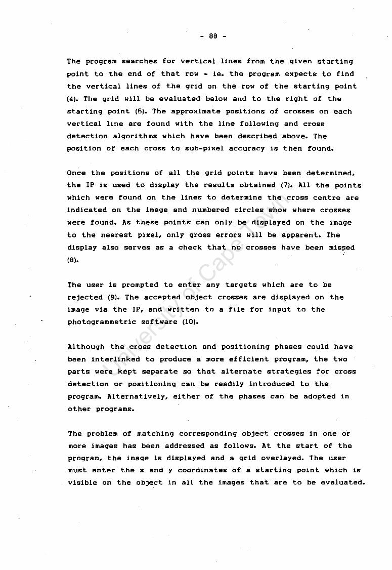
- 88 -
The program searches for vertical lines from the given starting
point to the end of that row - ie. the program expects to find
the vertical lines of the grid on the row of the starting point
(4). The grid will be evaluated below and to the right of the
starting point (5). The approximate positions of crosses on each
vertical line are found with the line following and cross
detection algorithms which have been described above. The
position of each cross to sub-pixel accuracy is then found.
Once the positions of all the grid points have been determined,
the IP is used to display the results obtained (7). All the points
which were found on the lines to determine the cross centre are
indicated on the image and numbered circles show where crosses
~ere found. As these points can only be displayed on the image
to the nearest pixel, only gross errors will be apparent. The
display also serves as a check that no crosses have been mis~ed
(8).
The user is prompted to enter any targets which are to be
rejected (9). The accepted object crosses are displayed on the
image via the IP, and writ ten to a file for input to the
photogrammetric software (10).
Although the cross detection and positioning phases could have
been interlinked to produce a more efficient program, the two
parts were k~pt separate so that alternate strategies for cross
detection or positioning can be readily introduced to the
program. Alternatively, either of the phases can be adopted in
other programs.
The problem of matching corresponding object crosses in one or
more images has been addressed as follows. At the start of the
program, the image is displayed and a grid overlayed. The user
must enter the x and y coordinates of a starting point which is
visible on the object in all the images that are to be evaluated.

- 89 -
Now, if grid points ar~ evaluated in two or more overlapping
images st~rting from the same object point, then corresponding I . . .
object crosses will have the, s-ame 'numbering in each of the
images. For each of the overlapping ,images, the. program will ,I j ~ • • I . ~ ,~ - ·"':'>
create a file which contains the cross· m.irnt:iei -:and its x "and y
coor'dinates.
, .
. .

- 91 -
two iterations for the original method, and after two and three
iterations for variations 1 and 2 respectively. These three ways
of finding a first approximation to the cross centre were
compared for 70 crosses. The following observations were made:
1. For all three methods, the deviations in the x and y
coordinates of the calculated cross centres from the true
cross centre had the same sign (ie. + or -) for all 70
crosses.
2. The weighted mean technique applied in the binary image
only, converged fastest and gave the best approximation to
the cross centre.
3. Variations 1 and 2 gave identical results for 80% of the
crosses. For the rest of the crosses the two variations
differed by a maximum of 0.9 pixels in x and o. 7 pixels in
Y• 4. The cross centre calculated with variations 1 and 2 was
always between 0.8 pixels in x and 0.3 pixels in y worse
than that obtained in the binary image.
5. Despite the differences in results obtained from the three
methods discussed in points 1-3 above, the first
approximation is usually the same when rounded to the
nearest pixel. The x and y coordinates rounded to the
nearest pixel are used as input for precise point
determination.
In conclusion, these observations illustrate ~hat there is '
nothing to be gained from the two variations which were tested,
because they are computationally more expensive and do not
improve accuracy.
8.2 Precision of Determining the Cross Centre
As described in chapter 7 the first step in determining the
precise position of a cross, is to determine two line points on

- 92 -
each cross arm. The distance along the cross arms where these
line points are determined depends on the first approximation of
the cross centre which is found during the detection phase.
However, as the weighted mean technique is used in the binary
image to determine this first approximation, this value can vary
for different thresholding values or lighting conditions. In order
to investigate how a-different first approximation affects the
final position of the cross, the starting point was moved through
a 3x3 kernel with its central pixel at the cross centre. For each
position, line points were found, polynomials fitted and their
intersection point found. The mean value of the nine values was
calculated and the deviations of each of the nine calculated
centres from this mean value was calculated. Table 8.1 shows the
maximum deviations in x and y for a nummber of crosses
investigated.
Cross no. max. deviation max. deviation in x (pixels) in y (pixels)
1 0.08 0.02· 2 0.03 0.02 3 0.38 0.02 4 0.38 0.01 5 0.30 0.30 6 0.27 0.06 7 0.28 0.06 8 0.02 0.23 9 0.38 0.28
10 0.03 0.02 11 0.10 0.06 12 0.10 0.02 13 0.10 0.02 14 0.02 0.01 15 0 .18 0.03 16 0.19 0.04 17 0.18 0.02
Table 8.1 Maximum deviations in x and y of the calculated cross position from the mean cross centre
Two conclusions may be drawn from these results. Firstly,
precision of the y coordinate is generally better than the

- 93 -
precision in the x coordinate, and by inspection, there is no
relationship between the two. Secondly, the precision of locating
a cross varies between 0.02 and 0.38 pixels. A precision of 0.05
pixels is considered to be good as it is equivalent to
approximately 0.75 microns in the image plane for PHOENICS.
The root cause of the large deviations is inaccurate line
determination. At first, it was thought that the weighted mean
technique can be applied and would yield satisfactory res.ults as
'the lines are well defined (ie. contrast) and are symmetrical in
. crossection in terms of grey shades. Al though these assumptions
are correct, the ratio of. grey values on a line to grey values
adjacent to a line is not . high enough (typically only 1.5 - 2). As
a result the weighted mean technique gives poor results if the
first approximation to the line centre is not good (Appendix E).
This can and does occur in practice. ,
In an·attempt to determine more precisely the centre of the . "' ~ . ..
line, a normal distribu~io.n c~~ve was fitted to the grey value
profile across a line using the least squares technique. Ref ering
to Fi(]. 8.1 it can be seen that t~e shape of t~e pixel intensity
prof He across a line is similar to . a. normal distribution curve. ~ . --
The axis of symmetry of the best-fit normal distribution curve
was considered to be t~~ line centre. This approach proved to be
unsuitable as again markedly different results w~re obtained for
different first approximations to the line centre.
----·--·--·- ---·- ----· .-

• --------------~----~------..,.!--"'-'~-:"" ........ ""· -
I
TE T SF'HERE
Fia. 8.2 Control fr~me and test •u~face

- 98 -
set up oloject In control frQMe
co.Mero. sto. tlon no.1 1
r-~---------------------------, I I I I I I I I I I I I I I I I I I I I
control frQMe
project unlforM light onto control frQMe
fMQQe cQpture with CCD ca.MerQs
oloject
project grid onto oloject
2 r1
I I I I I I I I I I I
3 .. :}
r1 r1
I I I
1
1
IMQge CQpture with 1
1 CCD CQMerQs I I I I I I I I I IMQge thresholding to IMQge thresholding to I I lsolQ te control points lsolQ te grid on oloject I f (IMQQe proccessor) (IMQQe proccessor) I I I I I I I I I I control point detection detection a.nd centering I I a.nd centering of conjugQte crosses I 1
<in-house softwa.re> with •cRoss• 1
I I I I 1
1
Identify conjugQte 1
1 control points results written to file I (Ma.nua.lly) I I I I I
~ -------:=~ ~o~r:,~:: :-o~J~C~---_-_-_-_-___ ...J _ _.._L...._...J __ L.._._~ •• • J Qnd control points (x, y>
photogrQMMetrlc softwQre
XYZ coordlnQtes of oloject points
3D coordlnQ tes of ~---~ control frQMe
Fig. 8.3 Surface measurement with PHOENICS
(1)
(2)
(3)
(4)
(5)
(6)

- 99 -
5. The images showing the control points (circular targets) and
those showing the object points (grid intersections) are
evaluated with separate computer programs. A computer
program written by Parkyn and Ruther is used to determine
the image coordinates of the control points. Conjugate
control points are then matched manually. The image
coordinates of conjugate object points are determined with
CROSS. CROSS is the computer pr~gram which implements the
cross det~ction, centering and matching algorithm
developed for this thesis.
6. Photogrammetric software written by Ruther is used to
determine th XYZ coordinates of the object points.
8.3.3 Results of Measuring the Test Surface
81 points on the sphere in a 9x9 grid were measured as descrµ:>ed
in 8.3.2 (see Appendix G for some sample images and Appendix I for
. a sample output of the photogrammetric software).
Analysis of the XYZ coordi~ates of the object points was done as
follows:
' 1. It was assumed that the a~tual surface was perfectly
spherical with a radius of 125.95 mm.
2. The ceritre coordinates of the best-fit sphere to the data
points was then determined using the least squares
technique assuming a fixed radius of 125.95 mm. This was
done with a computer program written by Ruther.
3. The normal distance from the surface to each data point
was determined by comparing the distance between the
centre of the sphere and the data points with the radius.
For the test sphere, the results obtained are summarised as
follows:

- 100 -
---~--
Distance between camera and sphere 1.5 m
Number of data points 81
Mean normal distance of data point from best-fitting sphere of radius 0.66 mm 125.95 mm
Sum of normal distances of data points to best-fitting sphere -0.01 mm
Standard deviation of measuring a 0.92 mm point on the sphere ( cJ ) ( * )
Table 8.2 Results of measuring the.test sphere with PHOENICS
(*) I
(I· normal distances btw. sphere and data points)2;e1 <· This represents the accuracy of measuring points with PHOENICS
at a distance of 1.5 m.

101
CHAPTER NiNE ''
• f ~ T t
9.0 . DISCUSSION OF THE ERRORS. AND LIMITATIONS OF· PHOENICS
" \, ..
The results of the two test stages show that. the developed cross , . ~
detection and ~entering al~orithm is effe6tive. The accuracy with
which points on a surface ·were measured was 0.92 mm at a
distance.~f 1.5.m and corresponds to a relative accuracy of
approximately i.:160~. This is acceptabe at the prototype stage of - -. . ... . . ' ~ .
PHOENICS and .is compa_7f'~1~;~.t~ sim~la':r .sy.st~~~ b~ing .. dev~i-~,red. ·
elsewh~re •.. In this chapter t~e accuracies and limitations of • • ., ii- • - I j t I ~ ....
PHOENICS are discussed. ( ·1 •
... J l - ·• V( :· • ~
9.1 Accur·acy Limitations in Measuring a Sur.face with PHOENICS .... \
Apart from errors which are a direct result of the cross
detection and centering algorithm, the measuring accuracy of • • -.. ": - ..... . .• 'i ~ • - ' • • " • • ' ' ~ • ' ',... -- ,
PHOENICS ,is. affected by.,, the .. following. 1'9'·· • . j • , • •.. ' - ..... • .
I'
1. Determination of the control field .,.: ..
:'"'.
The XYZ coordinates of the control points which had.a t • . . . ' • ( ' • , •
- diameter of 5 mm were measured with a reflex metrograph . , -~· ' h
with an uncertainty of 0.5 mm. If, for. example~ smaller I ' - 'P '!\ : ·, ., 4; I
targets are used,·the target centres can be estimated more
precisely and thus the coordinates of the points can be ' . .
determined with greater.accuracy. The limiting accur~cy of ~·( .. ... . - ; ~ . .
the ref lex metrograph is 0.1 mm.
2. Determination of image coordinates of the control points
.The algorithm which is presently be~ng ~sed to detetmine ~ ~. • • t. , 1 I ..., l
the centre of the circular control points can be described i ~ , ' · ·, .. ·:. "l · _ . ~ .... ' ..._ . •\ · .. I.• i . -~s
as follows: The extents of the target in the binary image - ".Jn - ·. ~ ·~ ,
are used to determine the size of a rectangular window . . '
around the target of which the weighted mean is . \.. / . _,
calculated in the real image. This value is taken as the
target centre. This means that that the size and/or the

- 103 -
s. Camera resolution and image size
Camera resolution directly affects the accuracy with which
the x and y coordinates of targeted points can be
determined in the image plane. Presently, cameras with a
highe~esolution than those used with PHOENICS are
avails~ but expensive. At the time of writing, a high
resolution CCD camera (lOOOxlOOO pixels) cost in excess of
ten times more than those used with PHOENICS (500x582
pixels). However, rapid advancement in the manufacturing
technology of CCDs is continually lowering the purchase
price. Furthermore, dimensionally larger pixel arrays which
have an even higher pixel density are being developed and
promise to significantly increase the accuracies that can
be achieved with CCD cameras.
6. Relative camera orientation and number of images
The test sphere was measured using two slightly convergent
images. If images from more than two camera positions are
used, the accuracy with which points are fixed in space
improves considerably. The photogrammetric software of
PHOENICS can evaluate the input of up to six images in a
single solution. RUther (1982) has shown that the best
results are obtained when the axes normal to the image
planes are at 90° to one another.
9.2 Limitations of Surface Measurement with PHOENICS
It has been stated earlier that the most important step in RTP
is the acquisition of images which are suitable for a specific
intended image processing operation. In particular, this refers to
the thresholded images which must be created so that targeted
points may be identified automatically. The creation of such
images without any operator assistance is a difficulty that has
as yet not been overcome with PHOENICS.

•
- 104 -
The experience that the writer has gained suggests that
retroreflective targets used in conjunction with a slide
projector (or any other suitable light source) is the simplest and
most effective method of creating scenes with highly contrasting
targeted points. This method was successfully used to generate
suitable images for automatic thresholding. Since only one light
source was used, the position and orientation of the cameras was
restricted. It is ideal to have a light source at each camera
station, or mounted to each camera.
Apart from this general problem, some of the present limitations
which are specific to the algorithm that was developed are given
below.
1. The object being measured may not change in depth by ~ore
than approximately 100 mm, as otherwise, the grid which is
projected onto the object will not be in focus over the
entire surf ace.
2. Adjacent crosses must be at least 20 pixels apart. The
density of crosses which can be found successfully with
the developed algorithm is directly proportional to the
camera's resolution. For the cameras used with PHOENICS,
the limiting distance between points on the object (ie.
projected grid intersections) which can be measured is
10 mm at an object-to-camera distance of 1~5 m. This means
that the ratio of grid spacing to the object-to-camera
distance may not be smaller than 1:150. An alternative to
higher resolution cameras is to decrease the diameter of
the small and large search-circles. However, this is not
recommended as it would reduce the reliability of the
algorithm •
3. Program execution is slow. For the test surf ace, fo~ which
81 crosses were detected and centered, the program ran for

- 105 -
20 minutes on the IBM PC. Hore expensive hardware such as
a 80386 processor in conjunction with parallel processors
will reduce execution time considerably.

- 106 -
CHAPTER TEN
10.0 CONCLUSIONS AND RECOMMENDATIONS
10.1 Conclusions
From the test results which were obtained and the discussion in
the previous chapter, the following conclusuions can be drawn.
1. The primary objective of the thesis was to develop a non
con tact measuring system for mapping sculptured surfaces
so that these can be represented by a set of XYZ
coordinates in. the form required by the milling system
developed by Back (1988). This was successfully completed. A
grid is projected onto an object with a slide projectq~ and
the XYZ coordinates of the surf ace at the grid
intersections are determined with PHOENICS.
2. An algorithm for the detection, centering and matching of
conjugate grid intersection points has been developed and
successfully tested.
3. The computer program which was written to implement the
developed algorithm can be reliably used as an image
matching tool with PHOENICS.
4. The non-contact surf ace measuring technique which was
developed was used in conjunction with the milling system
developed by Back (1988) to replicate a test object. This
test proved that the combined system is suitable for the
manufacture of "sculptured surfaces".
5. The accuracy requirements for the manufacture of medical
prostheses can be achieved with the combined measuring and
milling system. For example, at an object-to-camera
distance of 0.5 m, points on a surface can be measured

- 107 -
with an accuracy of approximately 0.3 mm at an interval of
5 mm. Back (1988) reported an average undercut ting error of
0.46 mm for the milling system. This combines to an
uncertainty of 0.55 mm.
6. The relative accuracy (absolute accuracy/distance) of
PHOENICS may be improved in a number of ways.
- more accurate determination of the control point
coordinates
- more accurate algorithms for determination of control
point image coordinates
- elimination or compensation for linejitter and other
electronic noise
- correction of lens distortion in the photogrammetric
software
- use of higher resolution cameras
- use of multiple images and optimal camera orientatioh
7. The use of retroreflective control point targets in
conjunction with a light source is the most effective way
of generating images suited to PHOENICS' algorithms for
automatic target detection.
10.2 Recommendations
As a result of the findings and conclusions of this thesis, the
following recommendations are made.
1. An investigation should be undertaken to determine whether
a more accurate method for determining the centre of a
line section will increase the accuracy of finding the
position of a cross centre. Frobin and Hierhol tzer (1983a)
and Davis (1988) present some algorithms which should be
investigated.

- 108 -
2. A complete error analysis of the PHOENICS measuring process
must be done.
3. Smaller control point targets must be used so that the
control field may be coordinated more accurately.
4. Investigation of target centering algorithms.
5. The CCD cameras of PHOENICS should be modified to
accoidf,date a suitable light source to be used in
conjunction with retroreflective targets.
6. Development and implementation of a control point matching_
algorithm.
10.3 Closing remarks
PHOENICS is an ongoing project and some of the above
recommendations are already being investigated. Presently, work is
being carried out in the following areas.
1. Improvement of the algorithm used for finding the centres
of the circular control targets.
2. Improvement of the photogrammetric software.
3. Development of user-friendly, front-end software which will
· integrate all the steps of surface measurement of
PHO ENI CS.
4. Introduction of parallel processors to PHOENICS in order to
decrease execution time.

- 109 -
In the near future, PHOENICS will be a fully operational, PC
based, NRTP vision system with a wide range of applications.

- 110 -
11.0 REFERENCES
American Society of Photogrammetry 1980. Manual of Photogrammetry. Fourth Edi ti on. Falls Church, Virginia: American Society of Photogrammetry, p. 1.
Ackermann, F. 1984. Digital Image Correlation: Performance and Potential Application in Photogrammetry. Potogram. Rec., Vol. 11, No. 64, pp. 429-439.
Adams, L. P. 1978. The Use of a Non-Metric Camera for Very Short Range Photogrammerty. Photogrm. Rec., Vol. 9, No. 51, pp. 405-414.
Adams, L. P. 1980. The Use of Short Range Photogrammetry in the study of the Shoebill Bill. Photogrammetric Record, Vol. 10, No. 55, pp. 73-84.
Adams, L. P. 1981. X-ray Photogrammetry for locating the precise, three-dimensional position of image points. Medical and Biological Engineering and Computing, Sept. 1981, No. 19 pp. 569-578.
Back, D. R. 1988. A Computer Aided Machining System for the Manufacture of Three-Dimensional Surfaces. Unpublished ·e.sc. Thesis. University of Cape Town, Dept. of Mechanical Engineering. 105 pp.
Badekas, J. 1974. Photogrammetric Surveys of Monuments and Sites. Proceedings of the First Symposium on Photogrammetric Surveys of Monuments and Sites, Athens (edited by J. Badekas), 176 PP•
Beyer, H. A. 1988. Lineji t ter and Geometric Calibration of CCD Cameras. International Archives of Photo. and R.S., Vol. 27, No. BlO, pp. V315-V324.
Berelowi tz, M. 1986. The Use of CAD/CAM in the Managemet of Orthopedic Patients. Unpublished B.Sc. Thesis. University of Cape Town, Dept. of Mechanical Engineering.
D~hler, J., 1986. Ladungsgekoppel te Elemente (CCD). Bericht Nr. 107, Institut fur Geod~sie und Photogrammetrie, ETH ~Urich,
35 pp.
Davis, M. 1988. Target Centering and Image Matching in a NRTP system. Unpublished B.Sc.( Hons) Thesis. University of Cape Town, Dept. of Applied Mathematics. 52 pp.
Duncan, J. P. and S. G. Mair 1983. Sculptured Surfaces in Engineering and Medicine. Cambridge University Press, Cambridge.

- 111 -
El Hakim, S. F. 1985. A Photogrammetric Vision System for Robots. Photogrammetric Engineering and Remote Sensing, Vol. 51, No. 5, pp. 545-552.
El Hakim, S. F. 1986. A Real-Time System for Object Measurement with CCD Cameras. International Archives of P. and R.S., Vol. 26, No. 5, pp. 363-373.
Frobin, w. and E. Hierholzer 1981. Rasterstereography: A Photogrammetric Method for Measurement of Body Surf aces. Photogrammetric Engineering and Remote Sensing, Vol. 47, PP• 1717-1724.
Frobin, w. and E. Hierholzer 1982. Calibration and Model Reconstruction in Analytical Close-range Photogrammetry, Part II. Photogrammetric Engineering and Remote Sensing, Vol. 48, No. 2, PP• 215-220.
Frobin, w. and E. Hierholzer 1983a. Automatic Measurement of Body Surfaces Using Rasterstereography, Part I. Photogrammetric Engineering and Remote Sensing, Vol. 49, No. 3, pp. 377-384.
Frobin, w. and E. Hierholzer 1983b. Automatic Measurement of Body Surfaces Using Rasterstereography, Part II. Photogramme~ric Engineering and Remote Sensing, Vol. 49, No. 10, pp. 1443-1452.
Frobin, w. and E. Hierholzer 1985. Simplified Rasterstereography Using a Metric Camera. Photogrammetric Engineering and Remote Sensing, Vol. 51, No. 10, pp. 1605-1608.
Gruen, A. 1985. Adaptive Least Squares Correlation - A Powerful Image Matching Technique. Presented Paper to the ACSM-ASP Convention, Washington, D. C., March 1985.
Gruen, A. 1986. The Digital Photogrammetric Station at the ETH Zurich. Paper Symposium ISPRS Commission 2, Baltimore, May 1986.
Gruen, A. 1987. Towards Real-Time Photogrammetry. Invited Paper, 41. Photogrammetric Week, Stuttgart, September 14-19, 33 p.
Gruen, A. W. and Beyer, H. A. 1987. Real-Time Photogrammetry at the Digital Photogrammetric Station (DIPS) of ETH Zurich. The Canadian Surveyor, Vol. 41, No. 2, pp. 181-199.
Haggren, H. 1986. Real-Time Photogrammetry as used for Machine Vision Applications. International Archives of Photogrammetry and Remote Sensing, Vol.26, No. 5, pp. 374-382.
Hirschberg, I. 1985. Advances in High-Resolution Imagers. Electronic Imaging, April 1985, pp. 56-62.

- 112 -
Keefe, M. and D. R. Riley 1986. Capturing Facial Surface Information. Photogrammetric Engine~ring and Remote Sensing, Vol. 52, No. 9, pp. 1539-1548.
Kntldler, G. and Kupke, H. 1974. The use of Industrial Photogrammetry in the Production of Ship's Screws. Jena Review, No. 3, 1974.
Luhmann, T. 1986. Ein Verfahren zur rotationsinvarianten Punktbestimmung. Bildmessund und Luftbildwesen, 54 (1986), Heft 4.
Luhmann, T. and Webster-Ebbinghaus, W. 1986. Rolleimetrics RS - A new system for digital image processing. Paper Symposium ISPRS Commission 2, Baltimore 1986.
Real, R. R., 1986. Components for Video-Based Photogrammetry of Dynamic Processes. International Archives of Photogrammetry and Remote Sensing, Vol. 26, No. 5, pp.432-444.
Real, R. R. and Y. Fujimoto 1986. Digital Video Stereoscopy: RealTime Instrumentation Issuses. Paper Symposium ISPRS Commission 2, Baltimore, May 1986.
Ruther, H. 1982. Re la ti ve Orientation with Limited Control. Unpublished Ph.D. Thesis. University of Cape Town, Dept. of Surveying.
Ruther, H. and Hall-Martin, A. 1979. Application of Stereo Photogrammetric Techniques for Measuring African Elephants. Koedoe, No. 22, pp. 187-198.
Ruther, H. and Parkyn, N. 1988. The Development of a PC-based Near-Real-Time Photogrammetry System - PHOENICS. International Archives of Photo. and R.S., Vol. 27, No. BB, PP• V105-V116.
Schild, W. 1988. Zeilen, Linien oder Megahertz?. Funkschau, September 1988, pp. 48-51.
Turner-Smith, A. R. and J. O. Harris 1986. Measurement and Analysis of Human Back Surface Shape. International Archives of Photo. and R.S., Vol. 26, No. 5, pp. 355-362.
Vaughn, C., G. Brooke, M. Price and J. Ireland 1986. The Micron Eye Toposcanner: A Versatile Anthropometric Instrument. Presented Paper, 2nd Annual Congress, Ergonomics.Society of Southern Africa, Cape Town.
Wong, K. W. 1986. Stereo Solid State Cameras. International Archives of Photogrammetry and Remote Sensing, Vol. 26, No. 5, PP• 454-458.

- 113 -
Wong, K. W. and Wei-Hsin Ho 1986. Close-Range Mapping with SolidState Cameras, Photogrammetric Engineering and Remote Sensing, Vol. 52, No. 1, pp. 67-74.
Wong, K. W. 1987. Real-Time Machine Vision Systems, The Canadian Surveyor, Vol. 41, No. 2, pp. 173-180.

- 114 -
12.0 BIBLIOGRAPHY
American Society of Photogrammetry 1980. Manual of Photogrammetry. Fourth Edition. Falls Church, Virginia: American Society of Photogrammetry, 1056 pp.
Wolf, P. R. 1983. Elements of Photogrammetry. Second Edition. Singapore: Mc Graw-Hill Book Co, 628 pp.
Moffit, F. H. and Mikhail, E. M. 1980. Photogrammetry. Third Edition. New York: Harper and Row, Inc., 648 pp.
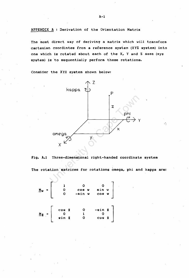
A-1
APPENDIX A Derivation of the Orientation Matrix
The most direct way of deriving a matrix which will transform
cartesian coordintes from a reference system (XYZ system) into
one which is rotated about each of the X, Y and Z axes (xyz
system) is 'to sequentially perform these rotations.
Consider the XYZ system shown below:
z ko.ppo.
p
z
phi y
y
Fig. A.1 Three-dimensional right-handed coordinate system
The rotation matrices for rotations omega, phi and kappa are:
[ 1 0 0 ] !!w = 0 cos w sin w 0 -sin w cos w
[ cos § 0 -sin § ] !!§ = 0 1 0 sin § 0 cos §

. [ cos k -sin k
0
sin k cos k
0
A-2
0 0 1 ]
The orienta~ion matrix M is then obtained by simply performing
the matrix multi plication !:!.w * !:!.§ * !:!.k to yield:
M = [
where: mu = cos§ * cosk
m12 = sin w * sin § * cos k + cos w * sin k
m13 = -cos w * sin § * cos k + sin w * sin k
m21 = -cos § * sin k
m22 = -sin w * sin § * sin k + cos w * cos k
m23 = cos w * sin § * sin k + sin w * cos k
m31 = sin §
m32 = -sin w * cos §
m33 = cos w * cos §

B-1
APPENDIX B Derivation of the Collinearity Equations
Collinearity is the condition which states that the exposure
station, an object point and its image point must all lie on a
straight line (see Fig. B.1). Here the image coordinates are xyz
and the object coordinates are XYZ.
The principal point has coordinates x0 , y 0 in the image space and
hence, the coordinates of any point 'a' in t.he image space are
(x - x 0 ), (y - y 0 ) relative to the principal point. x and y are
measured from an arbitrary origin on the image.
The exposure station has coordinates X0 , Y0 , Z0 in the object
space, and hence, the coordinates of a point 'A' corresponding to
the image point 'a' will have coordinates (XA - X0 ), (YA - Y 0),
(ZA - Z0 ) relative to the exposure station.
z
trlted plo.ne
Fig. B.1 Diagram of the collinearity condition
x
In order to develop the· condition equations, the image plane
must first be rotated so that its coordinate system is parallel

B-2
to that of the object space. This is done with the rotation
matrix M (derived in Appendix A) which has elements that are
functions of omega, phi and kappa (rotations about the x, y and z
axes). The new coordinate system (x'y'z') is shown in Fig. B.2.
z z'
rota. te d IMo.ge "'---- plo.ne
conto.lnlng the IMo.ge of A
x
Fig. B.2 Image coordinate system rotated so that it is
parallel to the object space
Thus
[
Xa - x 0 Ya - Yo za - Zo
x ' a Ya' z ' a
- Ko' ] - Yo• - Zo'
(B-1)
Using Fig. B.2 the collinear! ty con di ti on equations can be derived
from similar triangles subtended from the exposure station (0)
into the image and object space.

8-3
Thus
><a ' - Xo ' Ya ' - Yo ' Za ' - Zo ' = =
XA - Xo YA - Yo ZA - Zo
Or
><a ' = ((XA - Xo) I (ZA - Zo)) * (Za ' - Zo')
Ya ' = ((YA - Yo) I (ZA - Zo)) * (Za ' - Zo') (8-2)
Za ' = ((ZA - Zo) I (ZA - Zo)) * <za ' - Zo')
Expanding equation (8-1), substituting equations (8-2) and dropping
t.he 'a'/' A' subscript. (since A is an arbi t.rary point.), get.:
x - Xo y - Yo z - Zo x - ><o = <mu* + m12* + mi3* )*(z'-z 0 ')
z Zo z - Zo z - Zo
x - Xo y - Yo z - Zo y - Yo = <m21* + m22* + m23* )*(z'-z 0 ')
z - Zo z - Zo z - Zo
x - Xo y - Yo z - Zo z - Zo = (m31 * + m32* + m33* )*(z'-z 0 ')
z - Zo z - Zp z - Zo
Dividing equation (8-3) and (8-4) by (8-5) and noting that all
image points will have z' = -f (the focal length) yields:
mu(X - Xo) + mi2(Y - Yo) + m13(Z - Zo) x = (-f - z0 ) * + Xo
m31(X - Xo) + m32(Y - Yo) + m33(Z - Zo)
m21(X - Xo) + m22(Y - Yo) + m23(Z - Zo) y = (-f - z0 ) * +·Yo
m31(X - Xo) + m32(Y - Yo) + m33(Z - Zo)
.(8-3)
(8-4)
(8-5)
(8-6)

8-4
Now, multiplying out the parentheses, transposing x 0 , y 0 to the
right hand sides of the equations, and defining new constants,
equation (B-6) can be rewritten as:
bu *X + bi2*Y + b13*Z + b14 x =
b31 *X + b32*Y + b33*Z + 1
b21*X + b22*Y + b23*Z + b24 y = (B- 7)
b31 *X + b32*Y + bJ3*Z + 1
'
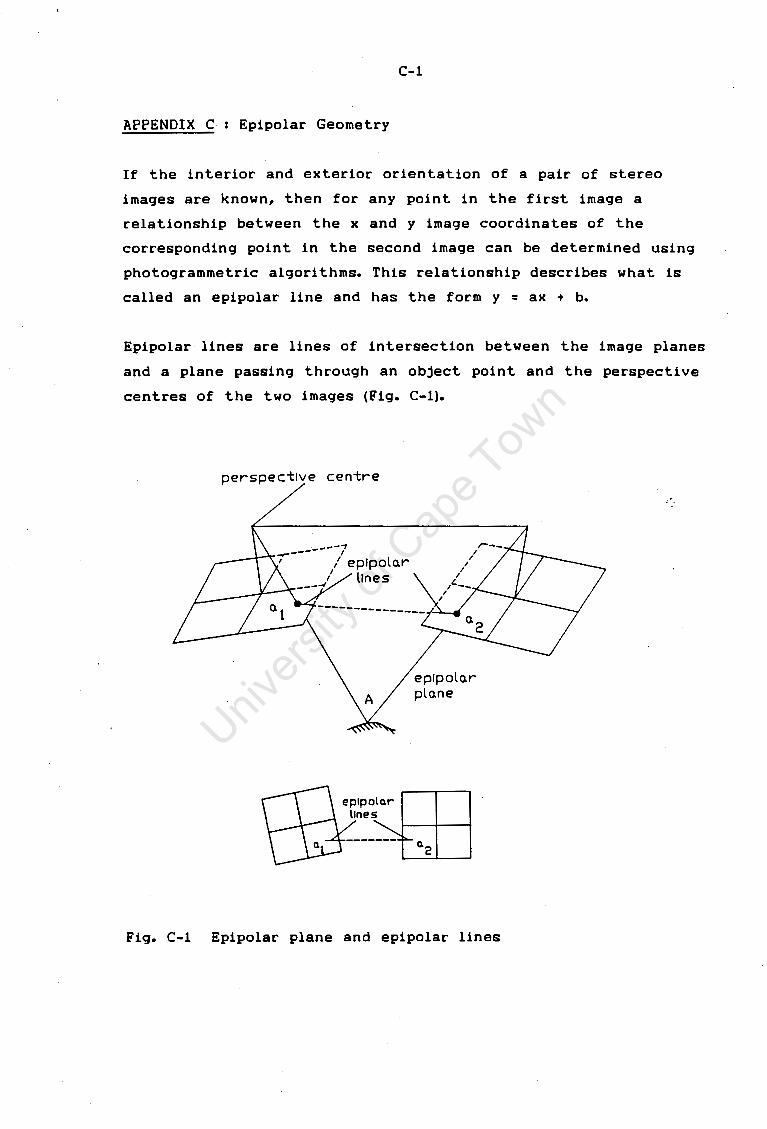
C-1
APPENDIX C Epipolar Geometry
If the interior and exterior orientation of a pair of stereo
images are known, then for any point in the first image a
relationship between the x and y image coordinates of the
corresponding point in the second image can be determined using
photogrammetric algorithms. This relationship describes what is
called an epipolar line and has the form y = ax + b.
Epipolar lines are lines of intersection between the image planes
and a plane passing through an object point and the perspective
centres of the two images (Fig. C-1).
perspective centre
eplpola.r pla.ne
Fig. C-1 Epipolar plane and epipolar lines

C-2
Any point on the object contained in the epipolar plane, will lie
on the epipolar lines in t.he images. Thus, for any object point
in image 1 (point A), its corresponding point in image 2 must lie
on the respective epipolar line (BC).

APPENDIX D
D-1
A Method of Interfacing the PIP Image Proccessing
Board with a Computer Language other than those
it supports
The PIP IP supports the MS-'C' and the MS-FORTRAN computer
languages. This means that the built-in functions of the IP can
be directly executed in a program written in either of these two
languages. With any other computer language, this is not possible.
In this thesis the software was written in TRUE BASIC. This meant
for example that the position of a cross that was detected and
its centre found, could not be displayed on the image. The image
could not be called up, nor could any of the IP graphics routines
be executed from a TRUE BASIC program. Thus there was no way of
easily checking the results obtained.
In order to check the results, it was neccessary to:
1. note the coordintes of the point
2. exit from TRUE BASIC
3. use the interpreter program of the IP (*) to call up the
particular image
4. use the graphics facilities of the IP to indicate the point
on the imge (two commands per point)
(*) The interpreter program of the IP (PIPINT.EXE) is a program
which allows the user to enter any of the IP functions from
the keyboard~
A way of using the IP from within a TRUE BASIC program was found
by the author.
When the interpreter program is executed, it automatically
searches for the file !NIT.PIP which contains the appropriate
interpreter commands to initialise the board to a desired state.
Any interpreter command in this file is automatically executed.
The !NIT.PIP file is a text file which the ,user can modify to.

D-2
suit his or her needs. All the interpreter commands must be in
lower case letters. The !NIT.PIP file can also be modified from
within a TRUE BASIC progra~ by specifying its organization as
"TEXT" in the "OPEN" statement. In TRUE BASIC the "OPEN"
statement associates a channel with a file saved on disk.
Once the !NIT.PIP file has been edited, all that remains to be
done is to run the interpreter program. There are two ways of
doing this:
1. A batch file is used in which first the TRUE BASIC program
is executed and then the interpreter program is run.
Example of commands in a batch file:
HELLO MYPROG.TRU (loads TRUE BASIC, execute.~5
PIPINT.EXE
"HYPROG.TRU" and returns to .DOS)
(runs the interpreter program
automatically executing the
commands in !NIT .PIP)
Note: Drive and path specifications have been omitted
here, but are neccessary.
2. The TRUE BASIC EXEC_RETURN subroutine is used in a TRUE
BASIC program. The EXEC_RETURN subroutine is contained in
the EXEC.TRC library file of the TRUE BASIC RUNTIME
PACKAGE. At the start of the program the statement
"LIRARY EXEC.TRC" must be included. In order to execute
the interpreter program, the subroutine EXEC_RETURN must
be called with argument "PIPINT.EXE" ie. as a program
statement: CALL EXEC_RETURN("PIPINT.EXE").
In the latter case it is recommended that the !NIT.PIP file .
contains as its last statement the "quit" command which will
terminate the interpreter program as the writers of TRUE BASIC

D-3
do not encourage the use of the EXEC_RETURN subroutine to run
"execute-and-stay-resident programs".

APPENDIX E
E-1
Evaluation of Using the Weighted Mean Technique for
Determining the Position of a Line-Section with
Sub-Pixel Accuracy
Typical pixel intensity profiles of two line sections are shown in
Fig. E.1. The position of the line section was taken to. be at the
peak of the best-fit curve to the data points. The curve was
generated with a CAD program which uses B-splines for curve
fit ting. The pixel intensity values are given in Table E.1 below.
Pixel intensity
Pixel position Line 1 Line 2
1 105 106 2 106 111 3 120 112 4 128 114 5 146 127 6 170 150 7 198 186 8 198 194 9 195 192
10 174 173 11 138 137 12 124 125 13 118 117 14 109 111 15 107 111
Centre of line 7.75 8.35
Table E.1 Pixel intensity values of two typical line sections
The weighted mean of an initial mask of 8 pixels was calculated.
This value was then used as the centre of the next mask. The
process was iterated until the position of the weighted mean
converged. This was done for a number of different positions of
the initial mask for both line sections. The results obtained are
tabulated in table E.2.

E-2
pixel Intensity
7.75
200
180
160
140
120
100 1 2 3 4 5 6 7 8 9 10 11 12 13 14 1 S:·
pixel nuMloer
LINE 1
pixel Intensity 8.35
180
160
140
120
100 1 2 3 4 5 6 7 8 9 10 11 12 13 14 15
pixel nuMloer
LINE 2
Fig. E.1 Pixel intensity profiles of two typical line sections

E-3
Position of line centre Deviation from approx. centre
(pixels) (pixels)
Centre Line 1 Line 2 Line 1 Line 2 of
initial 1st 2nd 1st 2nd mask iteration iteration
6 6.48 - 6.52 - -1.27 -1. 83 7 7.30 - 7.33 - -0.45 -1.02 8 7.98 - 8.09 - 0.23 -0.26 9 8.73 - 8.83 - 0.98 0.48
10 9.52 - 9.60 - 1. 77 1.25 11 10.39 9.52 10.45 9.6 1. 77 1.2~
Table E.2 Results of applying the weighted mean technique for
finding the position of a line section
From the results it became clear that this method is not
suitable for determining the position of a line section as it
does not converge. In addition, it only gives an acceptable
result if the first approximation to the line section is good. As
the thresholded image is used to determin~ the first
approximation,, it is quite possible that it will be one, or even
two, pixels from the "true" value.

F-1
APPENDIX F List of Computer Programs for use with PHOENICS
This Appendix contains a list of the computer programs which
have been written by the author and a brief explanation of their
use. These programs may be useful to future researchers. The user
is expected to have a working knowledge of DOS, TRUE BASIC, and
the PIP image processor. The neccessary background of PHOENICS
has been given in the main text.
F .1 TRUE BASIC Programs
These programs can be run using the TRUE BASIC compiler.
Program name
CROSS.TRU
IPLIB.TRU
IPLIB.TRC
VIEW.TRU
Cements
determines the position of grid intersecti~ns
in an image to sub-pixel accuracy. The
following files must be on disk:
CIRPOS_S.TRU
CIRPOS_L. TRU
SQUPOS_S. TRU
SQUPOS_L. TRU
CIRXY_S.TRU
CIRXY_L.TRU
IPLIB.TRC
EXEC. TRC (part of the TB RUNTIME package)
a library file containing image processing
routines - it cannot be run on its own.
compiled version of IPLIB.TRU
the pixel intensity values of a portion of an
image may be:
a. displayed on the computer screen
b. printed on the printer
c. writ ten to a text file for later
manipulation (eg. using LOTUS, VP-PLANNER)

INV_ALL.TRU
INV_BW.TRU
THRESH.TRU
CONCH.TRU
TR
RT
TR6
TR
RT
RED IT
REDITl
F-2
invert.s (in t.erms of colour) a grey image and
writ.es t.he result. t.o a file
invert.s (in t.erms of colour) a binary image and
writ.es t.he result to a file
thresholds an image and writes the result to a
file
computes the distance between two numbered
point~. The coordintes of the points must be
in a TRUE BASIC record file (recsize = 8) in t.he
following format: point number, X, 'i, z. converts a text file which contains numbered
x,y (image) coordinates to a record file (recsize
= 8) in the following format: point number, x,
y
converts a record file (recsize = 8) in the
format point number, x coordinate, y
coordinat.e, to a text. file
general text-to-record file conversion
converts a text file which contains numbered
x,y (image) coordinates to a record file (recsize
= 8) in the following format: point number, x,
y
converts a record file (recsize = 8) in the
format point number, x coordinate, y
coordinat.e, to a text file
allows the user to alter the point numbering
of image coordinates (x, y)in a record file
(recsize = 8)
allows the user to alter the point numbering
of space coordinates (X, 'i, Z) in a record file
(recsize = 8)
F.2 PIP Image Processor Macros
Certain desired functions which may be performed using t.he PIP
image processor require a sequence of commands to be entered at

F-3
the keyboard. Such a sequence of commands may be written to a
file (macro) and stored. A macro can be recalled later and
executed.
A list of the macros which have been writ ten is given below.
Program name
CAM.
CAM.R
CWR.R
CWRT.R
ITHI(.R)
ITHO(.R)
NEGI ( .RJ
NEGO ( .R)
NORMI(.R)
NORMO ( .R)
OWR.R
Cements
camera initialised on current board
cameras initialised on both boards
the contents of "quad O" of boards "0" and "1"
are writ ten to the files "ciml" and "cim2"
respectively - grey images of control points
the contents of "quad O" of boards "O" and "1"
are writ ten to the files "cimtl" and "cimt2"
respectively - binary images of control points
image is thresholded and inverted (in terms of
colour) at image capture (input), the user is
prompted for the thresholding value
image is thresholded and inverted (in terms of
colour) at the display (output), the user is
prompted for the thresholding value
the image is inverted (in terms of colour) at
image capture (input)
the image is inverted (in terms of colour) at
the display (output)
the image is normalised at image capture
(input) ie. any previous commands/macros which
alter the input are neutralised
the image is normalised at image display
(output) ie. any previous commands/macros which
alter the output are neutralised
the contents of "quad 0" of boards "O" and "1"
are written to the files "oiml" and "oim2"
respectively - grey images of object points
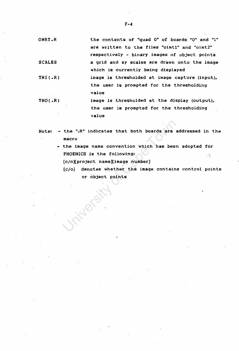
OWRT.R
SCALES
THI(.R)
THO( .R)
F-4
the contents of "quad 0" of boards "0" and "1"
are written to the files "oimtl" and "oimt2"
respectively - binary images of object points
a grid and xy scales are drawn onto the image
which is currently being displayed
image is thresholded at image capture (input),
the user is prompted for the thresholding
value
image is thresholded at the display (output),
the user is prompted for the thresholding
value
Note: - the ".R" indicates that both boards are addressed in the
macro
- the image name convention which has been adopted for
PHOENICS is the following: .
[c/o][project name][image number]
[c/o] denotes whether the image contains control points
or object points
\

APPENDIX G
G-1
A Set of Typical Images which were used for Surface
Measurement with PHOENICS
For each camera station there are four images: A grey and a
thresholded image of the control field to determine the control
point coordinates, and a grey and a thresholded image of the
object to determine the object point coordinates. At present it
is neccessary to have separate images of the control frame and
the object, since it is difficult to obtain an image from which
control and object points can be determined. Furthermore, the
algorithms for point determination and matching of the two
different types of targets (circular and cross shaped) have been
developed independently.
The images shown in this Appendix were taken from two different
camera positions and have been labeled "left" and "right". Fig~ __ G.7
shows the grid and scales which are overlayed to assist the user
when prompted to enter a starting point for the image search at
the start of the CROSS program.

t
I·
• ;;'
'
t.
• I
~ .
'
'
v !
• ~r t,._: t • ........ "·."·· ··-. ~ .
G-2
41·
-p
•
~t I ,,
<tl·· t. y
, .. :...tu..."·
'
~ ~
'
~ I
(
I ~
' ( (
c. .c ..., tJI c . .... c ..... E L a + a 't
I. ( ~
+ ~ a
<l t: ct f
:> <l L
C!
-• ~

• • •
• •
• ...
G.2 Thresholded imaqe Cleft) for determininn +hQ ~nn+n1 nnin+~
• •
••
•
~ I w

·i:
t '
I
. I ,.
.....
··~·
~"'t- ! ' .~, , ... , .•. '1 •
···.:. : ·~
--
.. ... ..
. .', ::'::'·" ..... 1,:-.:.·'"
.;:; .
j·~.......-,. '
•• oJ ..
,.J--li--1--i~+-i~ ..... -'ti .. -r-~·-·· . ., . .1 .. . i
: I
j , ...... .J ' .. _ .. ...::_ ....
~~--,.;,; ..... ...,..."'""'""
G.3 Grey image (left) for determining the obiect points
.. .. ......
-
1
Iii . ~¥. f {
·....,_
.;..
-···1 .I"
"'·'

I
-
'
•.'
G.4 Thresholded image (left) for determinina the obie~t nn; n t ~
G1 I
U'I

G-6
·-l1
·~ . '"
' ~ ' ..
:f• - •
t'l ~ c: .... 0 0
-c s.. ..... c c l)
Q) .c .µ
tJ'I c . ... c .... E
'"' QJ ~ QJ ,, '"' 0
<I-I
U") . C!7

G.6
;•
•" ·., ~o T' 1.,.. - . -.. ,,, ··~·
-
'.
! :~.:.~
,-
; :,< · ... ,
,. .... ~ J.
.. .. . ... II!' •
···If!! ~,.,... ·,
.,,_:,:11-•
:~ . "4~· '
"'!-
. ...,,.,
- J
··-.. 1..:J~~~~.~~,·~ .. ,··~;-.·-,.-.-,tr;~~::J~·~,.~,._·;:~:r~,:',~~~~:~· 1r'~!;f~iTj1·r\·:;~;:=~~~!·,.'~~'.:~~~'::1; ... -.,; •. =.·=1~-·::,., ~ t*· ,; 1' , .,... : .,J:. ·r.;;l :if ·, :- 9· · •·.
!~~I !:' 1.Jr.. ~.... '!J.~. r... .~~}i.
·'1.
. '·
I
• ~-
if.,,.,,.._,.~ollliU.,'111"°'' ~---"'"''-•w+11 .. ~·~...;..-.. ·...:... ii"
· .. ~ ..
Grey irnaqe (riqht) for determining t hA nh;A .... + nni nt !":
•·

•• I
·~;ii;, .. :J;;:~;·rt ·<,+!~·:·: .... ~.,-:- ,.. ~:.p.;.:~~·=··· .
· ·~1~'!!:--s!1~~~~~w:::~~!' -~·· ~~~,IJP·"':
, ,. ,, ..-;
•
•
·•
• .:
',:··=-· ? .. , ...
·. •'!': ::..
,,··
. I
G.7 Image for determining the object points with a graduated qrid overlaved
<il I a>

H-1
APPENDIX H Coordinates of the Control Frame
Control Coordinates of control points (mm) point number x y z
1 286.52 19.16 116.56 2 298.50 147.47 115.57 3 286.05 287.68 118.09 4 259.30 49.38 17.31 5 270.56 152.66 17.86 6 261.22 260.03 19.25 7 151.01 17.09 118.15. 8 156.73 43.56 19.35 9 154.04 257.94 21.55
10 156.13 290.16 121.25 11 52.24 48.35 20.03 12 38.91 155.41 20.99 13 56.56 258.94 22.79 14 23.06 18.07 118.13 15 7.80 155.58 116.97 16 19.95 289.90 119.57
Table H.1 Coordinates of control frame
I

• I
H-2
Fiq. H.1 Numbering of control frame

I
I-1
APPENDIX I Sample Output of Photogrammetric Software for the
Test Sphere
- The algorithm of the 11-PARAMETER-TRANSFORMATION which is
used in the photogrammetric software is outlined in section
2.5 of the main text.
Space Coordinates of Control Points
x y z
1 286.517 19.157 116.555 2 298.498 147.472 1i5.568 3 286.050 287.682 118.092 4 259.300 49.383 17.315 5 270.555 152.655 17.860 6 261.218 260.028 19.247 7 151.013 17.087 118.153 8 156.728 43.560 19.350 9 154.040 257.938 21.550
10 156.130 290.157 121.248 11 52.242 48.352 20.033 12 38.910 155.413 20.990 13 56.562 258.938 22.788 14 23.057 18.068 118.133 15 7.802 155.578 116.968 16 19.948 289.905 119.572
Image Coordinates of Control Points
Image 1 x y
1 99.020 32.790 2 251.460 16.060 3 412.440 48.180 4 144.760 70.180 5 273.950 55.580 6 405.480 78.110 7 93.280 260.620 8 134.030 254.910 9 400.060 265.600
10 410.450 260.630 11 136.050 442.550 12 270.470 466.750 13 396.740 435.160 14 92.130 475.640 15 253.280 502.010 16 406.870 481.710
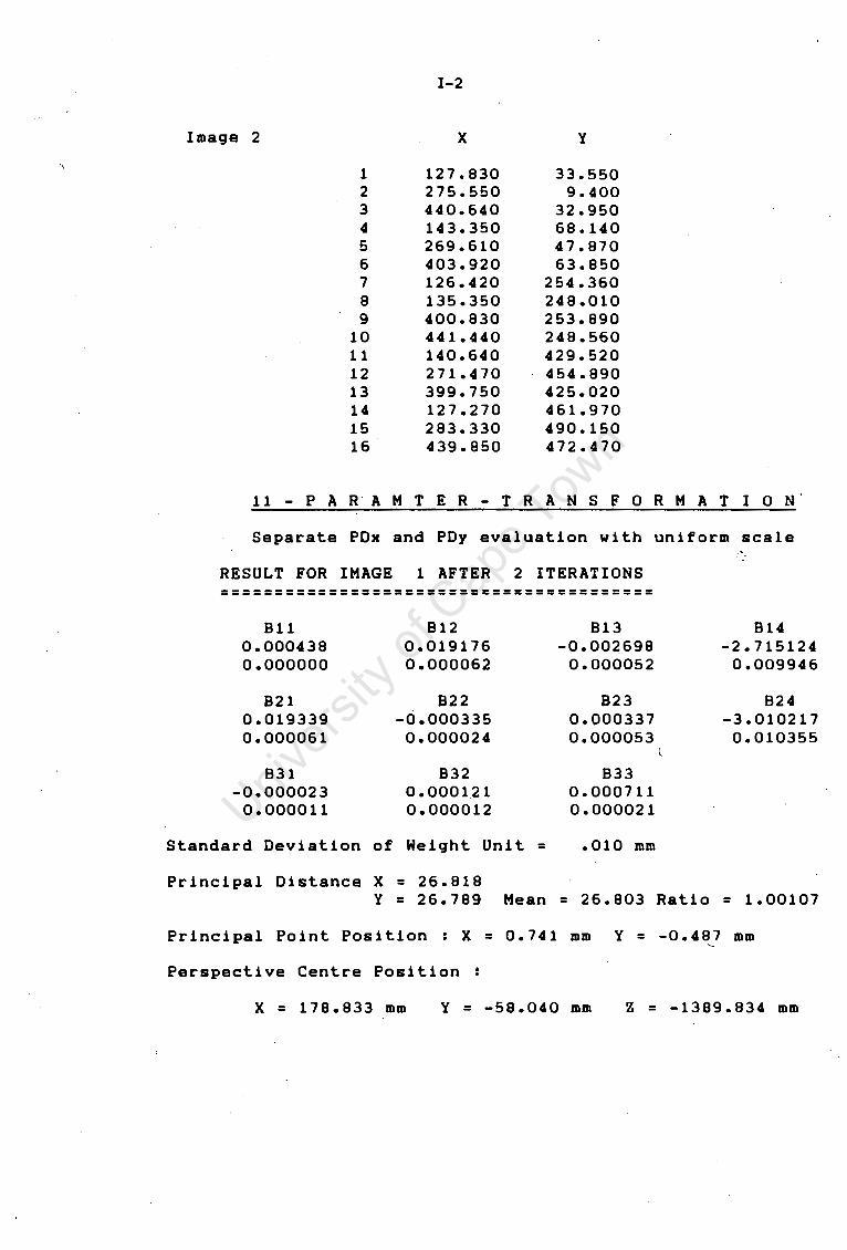
Image 2
1 2 3 4 5 6 7 8 9
10 11 12 13 14 15 16
I-2
x
127.830 275.550 440.640 143.350 269.610 403.920 126.420 135.350 400.830 441.440 140.640 271.470 399.750 127.270 283.330 439.850
'i
33.550 9.400
32.950 68.140 47.870 63.850
254.360 248.010 253.890 248.560 429.520 454.890 425.020 461.970 490.150 472.470
11 - P AR. A M T E R - T R A N S F 0 R M A T I 0 N'
Separate PDx and PDy evaluation with uniform scale
RESULT FOR IMAGE 1 AFTER 2 ITERATIONS ========================================
811 812 813 814 0.000438 0.019176 -0.002698 -2.715124 0.000000 0.000062 0.000052 0.009946
821 822 823 824 0.019339 -0.000335 0.000337 -3.010217 0.000061 0.000024 0.000053 0.010355
(
831 832 833 -0.000023 0. 0001.21 0.000711
0.000011 0.000012 0.000021
Standard Deviation of Weight Unit = .010 mm
Principal Distance X = 26.818 'i = 26.789 Mean = 26.803 Ratio = 1.00107
Principal Point Position : X = 0.741 mm 'i = -0.487 mm '-
Perspective Centre Position :
X = 178.833 mm 'i = -58.040 mm Z = -1389.834 mm

I • • • •
• -• I •
\
I-3
CONTROL POINT IMAGE COORDINATES AND CORRECTIONS FOR IMAGE 1
No x vx y vy mm mm mm mm
1 -2.355 -0.006 2.366 0.026 2 -0.068 -0.003 2.543 -0.011 3 2.347 0.001 2.203 -0.014 4 -1.669 -0.006 1.970 o.ooo 5 0.269 0.012 2.124 o.ooo 6 2.242 -0.004 1.886 -0.002 7 -2.441 0.006 -0.049 -0.001 8 -1.830 -0.002 0.012 0.002 9 2.161 -0.001 -0.102 -0.007
10 2.317 0.013 -0.049 0.004 11 -1.799 -0.005 -1.977 0.008 12 0.217 -0.014 -2.234 -0.005 13 2.111 -0.001 -1.899 -0.004 14 -2.458 0.008 -2.328 0.003 15 -0.041 0.003 -2.608 0.002 16 2.263 -0.001 -2.393 -0.001
:"".
RESULT FOR I HAGE 2 AFTER 2 ITERATIONS ========================================
811 812 813 814 0.000108 0.018431 0.002105 -2.675262 0.000000 0.000056 0.000049 0.009450
821 822 823 824 0.018550 -0.000086 0.000337 -2.823751 0.000054 0.000022 0.000048 0.009229
831 832 833 -0.000039 -0.000071 0.000692
0.000010 0.000011 0.000019
Standard Deviation of Weight Unit = .009 mm
Principal Distance X = 26.605 Y = 26.591 Hean = 26.598 Ratio = 1.00054
Principal Point Position : X = 0.299 mm Y = -1.011 mm
Perspective Centre Position :
X = 179.109 mm Y = 304.308 mm Z = -1402.687 mm

I-4
CONTROL POINT IMAGE COORDINATES AND CORRECTIONS FOR IMAGE 2
No x vx y vy mm mm mm mm
1 -1.923 -o.ooa 2.358 0.024 2 0.293 0.002 2.614 -0.014 3 2.770 -0.007 2.364 -0.010 4 -1.690 -0.003 1.991 -0.002 5 0.204 -0.001 2.206 .;.0.000' 6 2.219 0.014 2.037 o.ooo 7 -1.944 -0.002 0.011 -0.001 8 -1.810 -0.004 0.085 -0.005 9 2.172 0.011 0.022 0.004
10 2.782 0.006 0.079 0.003 11 -1.730 -0.005 -1.839 0.006 12 0.232 -0.009 -2.100 -0.003 13 2.156 -0.005 -1.792 -0.004 14 -1.931 0.006 -2.183 0.001 15 0.410 0.005 -2.482 0.003 16 2.758 -0.001 -2.295 -0.002
Calculated Space Coordinates using 11-Parameter Solution
Calculated Values of Control Discrepancies Images (calculated - real) used
x y z dX dY dZ
1 285.856 18.964 115.425 -0.661 -0.193 -1.130 2 2 299.872 147.067 115.208 1.374 -0.405 -0.360 2 3 285.266 287.797 118.186 -0.784 0.115 0.094 2 4 259.338 50.055 17.797 0.038 0.672 0.482 2 5 270.558 152.425 18.625 0.003 -0.230 o.765 2 6 261.184 259.941 19.808 -0.034 -0.087 o.561 2 7 151.122 17.067 120.156 0 .109 -0.020 2.003 2 8 156.698 43.735 17.674 -0.030 0.175 -1.676 2 9 154.256 258.550 21.221 0.216 0.612 -0.329 2
10 155.800 289.961 120.564 -0.330 -0.196 -0.684 2 11 51.934 47.703 21.021 -0.308 -0.649 0.988 2 12 38.759 155.227 20.193 -0.151 -0.186 -0.797 2 13 56.961 258.647 22.729 0.399 -0.291 -0.059 2 14 23.196 18.489 117.766 0.139 0.421 -0.367 2 15 7.716 155.534 117.032 -0.086 -0.044 o.064 2 16 20.044 290.190 120.020 0.096 0.285 0.456 2

I-5
Image Coordinates of Object Points
Image 1 x y
1 192.053 162.512 2 193.024 184.880 3 194.080 208.464 4 194.256 232.006 5 195.503 256.174 6 195.396 280.352 7 194.904 305.133 8 195.000 329.564 9 194.506 354.616
10 209.856 161.013 11 210.872 183.854 12 212.093 207.353
• • • • • •
81 330.477 351.847
Image 2 x y
1 210.911 156.161 \ 2 209.844 178.224
3 208.962 201.135 4 208.126 224.123 5 208.104 247.833 6 208.383 271.635 7 208.792 295.835 8 209.724 319.822 9 210.593 344.235
10 226.534 154.144 11 225.320 176.670 12 224.744 199.752
• • •
• 81 346.234 341.256

I-6
OBJECT POINT IMAGE COORDINATES AND CORRECTIONS
Point Image x vx y vy mm mm mm mm
1 1 -0.959 -o.ooo 0.991 -0.002 2 -0.676 -o.ooo 1.058 0.002
2 1 -0.945 -o.ooo 0.754 -0.001 2 -0.692 o.ooo 0.824 0.001
3 1 -0.929 -o.ooo 0.504 -0.002 2 -0.706 o.ooo 0.582 0.002
4 1 -0.926 -o.ooo 0.254 -0.002 2 -0.718 o.ooo 0.338 0.002
5 1 -0.907 -o.ooo -0.002 -0.002 2 -0.718 o.ooo 0.087 0.002
6 1 -0.909 -0.000 -0.258 -0.001 2 -0.714 o.ooo ' -0.166 0.001
7 1 -0.916 -o.ooo -0.521 -0.002 2 -0.708 o.ooo -0.422 0.002
8 1 -0.915 -0.000 -0.780 -0.001 2 -0.694 o.ooo -0.677 0.002
9 1 -0.922 -o.ooo -1.045 -0.002 2 -0.681 o.ooo -0.935 o. 00,2
10 1 -0.692 -o.ooo 1.007 -0.002 2 -0.442 -0.000 1.000 0.002
11 1 -0.677 -o.ooo 0.765 -0.001 2 -0.460 o.ooo 0.841 0.001
12 1 -0.659 -o.ooo 0.516 -0.001 2 -0.469 o.ooo 0.596 0.001
• • • • • • • • • •
• 81 1 1.117 -0.000 -1.016 -0.001
2 1.354 o.ooo -0.904 0.001

I-7
Calculated Space Coordinates of Object Points
x '{ z 'Images used
1 210.631 95.598 87.239 2 1 2 2 197.423 95.858 79.330 2 1 2 3 183.736 96.231 71. 795 2 1 2 4 170.140 96.205 67.402 2 1 2 5 156.244 96.979 62.231 2 1 2 6 142.258 97.228 62.556 2 1 2 7 127.898 97.349 64.573 2 1 2 8 113.664 97.934 66.447 2 1 2 9 98.975 98.226 70.050 2 1 2
10 211.715 109.699 81.192 2 1 2 11 198.267 109.857 72.675 2 1 2 12 184.614 110.358 65.706 2 1 2
• • • • • • • • • • • • •
81 101.643 212.023 72.168 2 . 1 2 -· :"'.
3 0 JUN 1989