SUPPORTING RESULTS: Figures S1-S6, Tables S1-S3amink/publications/manuscripts/... · Smith et al 8 SUPPORTING METHODS: Protocol S1, Figures S7 and S8 Electrophysiology Experiments

Smith et al

1

Supporting Information

for Smith et al. 2006, PLoS Computational Biology 2:e161

SUPPORTING RESULTS: Figures S1-S6, Tables S1-S3

Electrode Locations

HF

Cb

NCML3

L2L1

CMM

HA

M

S CSt

CSt

Cb

NCML3 L2 L1

CMM

HA

HF

HF

NCML3 L2 CMM

HA

SM

Cb

1 mm

Bird 3 (Black747)

Bird 6 (DGrA350)

Bird 4 (LtGr841)

Bird 5 (Pur10)

Bird 2 (Pur219)

Bird 1 (Red648)

1mm 1

23

4567

8

G

A

B

C

D

E

Figure S1. Electrophysiological recordings. (a) Female zebra finch with implanted electrodes. (b) Removed skull of

one bird showing below it the 8 implanted electrodes and ground wire. (c-e) Approximate locations of all electrodes

in all birds. Drawings represent sagittal sections at (c) ~0.4 mm, (d) ~0.6 mm; and (e) ~0.8 mm from the midline.

Electrode locations from different birds are indicated with different symbols. The lateral striatum (LSt) electrode of

bird 5 was in a plane further lateral than our drawings. The CSt electrode of bird 2 is in a plane between d and e.

The front of the brain is to the right and the dorsal part is to the top. Abbreviations are as in Fig. 1 of the main text,

with additional terms S-septum; HA-hyperpallium apicale; HF-hippocampal formation, and M-mesopallium.

Smith et al

2

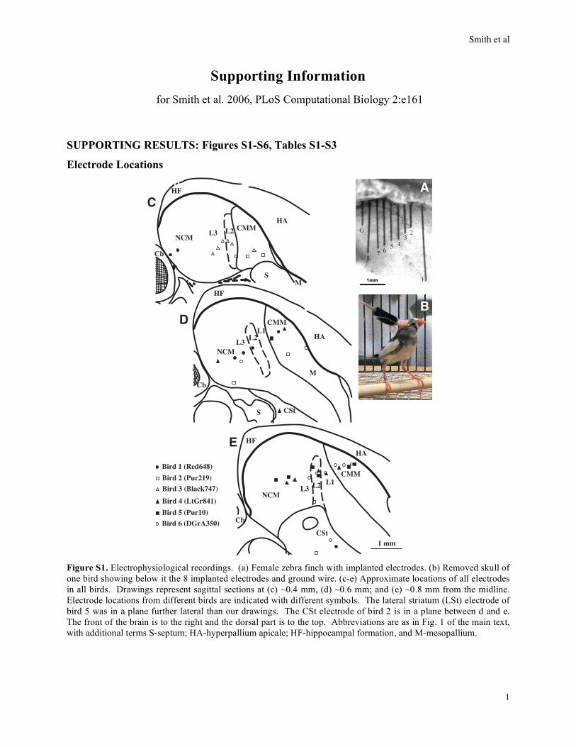
Fig

ure

S2

. S

ign

ific

ant

inte

racti

on

s w

hen

meas

ure

men

ts f

rom

all

six

bir

ds

(each

co

lore

d w

ith

a d

iffe

ren

t co

lor:

bir

d #

1 i

s re

d, #

2 p

urp

le, #

3 g

rey

, #

4 y

ell

ow

,

#5

pin

k, an

d #

6 g

reen

) w

ere p

oo

led

to

geth

er (

46

ele

ctr

od

es)

alo

ng

wit

h o

ne

no

de

rep

rese

nti

ng

th

e so

un

d s

tim

ulu

s: a

bin

ary

var

iab

le i

nd

icat

ing

th

e si

len

t

ver

sus

sou

nd

po

rtio

n o

f th

e st

imu

lus.

Nu

mb

ers

nex

t to

each

lin

k r

epre

sen

ts t

he

nu

mb

er o

f ti

mes

it

rep

eate

d a

cro

ss t

he 1

2 n

etw

ork

s (a

s o

ne b

ird

had

data

fro

m

on

ly 3

day

s, t

his

an

aly

sis

was

do

ne u

sin

g o

nly

th

ese

thre

e d

ay

s fo

r all

bir

ds)

, an

d l

ink

th

ick

nes

s is

sca

led

to

th

e s

qu

are o

f th

is v

alu

e. A

s can

be s

een

fro

m t

he

fig

ure

, n

o l

ink

s w

ere

fou

nd

betw

een

ele

ctr

od

es i

n d

iffe

ren

t b

ird

s, a

nd

no

lin

ks

wer

e fo

un

d into

th

e so

un

d s

tim

ulu

s v

aria

ble

.

Com

bin

ed A

naly

sis

of

All

Bir

ds’

Ele

ctro

des

Plu

s S

ou

nd

Smith et al

3

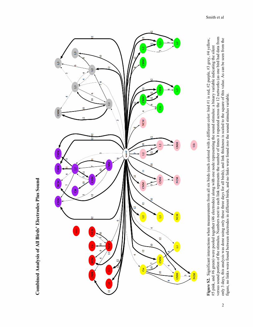
Analysis of Data from Subsections of Stimuli

Bird 4 - LtGr841

offset transition

NCM L1NCM L3 CMM CMM CStL2

onset transition


silence after sound


during sound


entire stimulus


silence before sound


Bird 5 - Pur10

offset transition

NCMNCM CMM CMM LStL2 L2 CMM

onset transition


silence after sound


during sound


entire stimulus


silence before sound


Figure S3. Networks inferred from subsections of data across all stimuli, in comparison with entire stimuli, for two

example birds. Consistent interactions are shown as described in legend of Figure 2c, main text.

Smith et al

4

Statistics in the table below (and all subsequent tables) are organized such that if there is an entry

in column i and row j, it means that the value of the variable for condition i is greater than that for

condition j. The entry indicates how statistically significant this difference is. Since the value for

i is greater than j, it follows that the value for j cannot be greater than i, and there is no entry in

column j and row i.

Table S1. Statistics for analysis of subsections of stimulus from main text and Figure 3b and c.

Comparison of number interactions for each subsection (main text)

ANOVA: F4,20=0.5, P=0.7, repeated measures

No pair-wise comparisons performed, due to non-significant ANOVA

Comparison of number of links per network for each subsection (Fig. 3b)

ANOVA: F4,344=124.5, P<0.0001, repeated measures, controlled for bird

Bonferonni-corrected pair-wise comparisons:

stimulus

subsections:

(silence)

before

(sound)

during

(silence)

after

onset offset

before - P<0.001* P<0.001*

during P=0.013* P>0.5 P<0.001* P<0.001*

after P>0.5 - P<0.001* P<0.001*

onset - - - -

offset - - - P=0.3

Comparison of percent of interactions matching interactions from entire stimulus for each subsection (Fig.

3c; main text)

ANOVA: F4,20=2.3, P=0.09, repeated measures


Comparison of percent of links matching interactions from entire stimulus for each subsection (main text)

ANOVA: F4,304=2.0, P=0.09, repeated measures, controlled for bird


Asterisks (*) indicate significant differences. A P-value in a cell indicates that the percent of links for the stimulus

subsection for that column is greater than for that row. For example, the number of links for ‘onset’ subsection is

greater than the number for ‘before’ subsection at P<0.001.

Smith et al

5

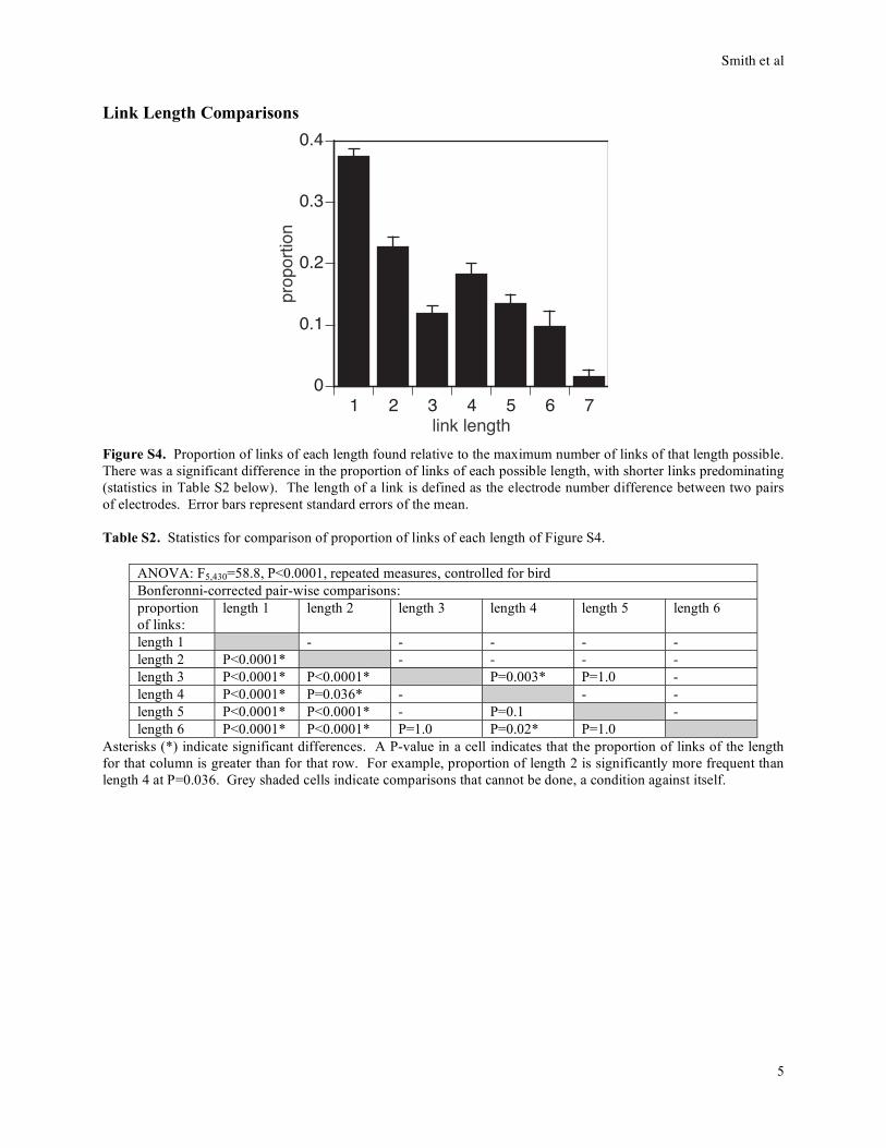
Link Length Comparisons

1 2 3 4 5 6 70

0.1

0.2

0.3

0.4

prop

ortio

n

link length

Figure S4. Proportion of links of each length found relative to the maximum number of links of that length possible.

There was a significant difference in the proportion of links of each possible length, with shorter links predominating

(statistics in Table S2 below). The length of a link is defined as the electrode number difference between two pairs

of electrodes. Error bars represent standard errors of the mean.

Table S2. Statistics for comparison of proportion of links of each length of Figure S4.

ANOVA: F5,430=58.8, P<0.0001, repeated measures, controlled for bird

Bonferonni-corrected pair-wise comparisons:

proportion

of links:

length 1 length 2 length 3 length 4 length 5 length 6

length 1 - - - - -

length 2 P<0.0001* - - - -

length 3 P<0.0001* P<0.0001* P=0.003* P=1.0 -

length 4 P<0.0001* P=0.036* - - -

length 5 P<0.0001* P<0.0001* - P=0.1 -

length 6 P<0.0001* P<0.0001* P=1.0 P=0.02* P=1.0

Asterisks (*) indicate significant differences. A P-value in a cell indicates that the proportion of links of the length

for that column is greater than for that row. For example, proportion of length 2 is significantly more frequent than

length 4 at P=0.036. Grey shaded cells indicate comparisons that cannot be done, a condition against itself.

Smith et al

6

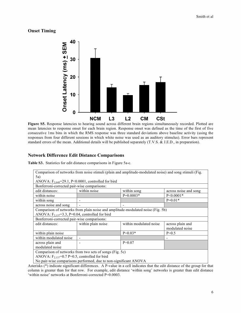
Onset Timing

Figure S5. Response latencies to hearing sound across different brain regions simultaneously recorded. Plotted are

mean latencies to response onset for each brain region. Response onset was defined as the time of the first of five

consecutive 1ms bins in which the RMS response was three standard deviations above baseline activity (using the

responses from four different sessions in which white noise was used as an auditory stimulus). Error bars represent

standard errors of the mean. Additional details will be published separately (T.V.S. & J.E.D., in preparation).

Network Difference Edit Distance Comparisons

Table S3. Statistics for edit distance comparisons in Figure 5a-c.

Comparison of networks from noise stimuli (plain and amplitude-modulated noise) and song stimuli (Fig.

5a)

ANOVA: F2,648=29.1, P<0.0001, controlled for bird

Bonferroni-corrected pair-wise comparisons:

edit distances: within noise within song across noise and song

within noise P=0.0003* P<0.0001*

within song - P=0.01*

across noise and song - -

Comparison of networks from plain noise and amplitude-modulated noise (Fig. 5b)

ANOVA: F2,137=3.3, P=0.04, controlled for bird

Bonferroni-corrected pair-wise comparisons:

edit distances: within plain noise within modulated noise across plain and

modulated noise

within plain noise P=0.03* P=0.5

within modulated noise - -

across plain and

modulated noise

- P=0.07

Comparison of networks from two sets of songs (Fig. 5c)

ANOVA: F2,137=0.7 P=0.5, controlled for bird


Asterisks (*) indicate significant differences. A P-value in a cell indicates that the edit distance of the group for that

column is greater than for that row. For example, edit distance ‘within song’ networks is greater than edit distance

‘within noise’ networks at Bonferroni-corrected P=0.0003.

Smith et al

7

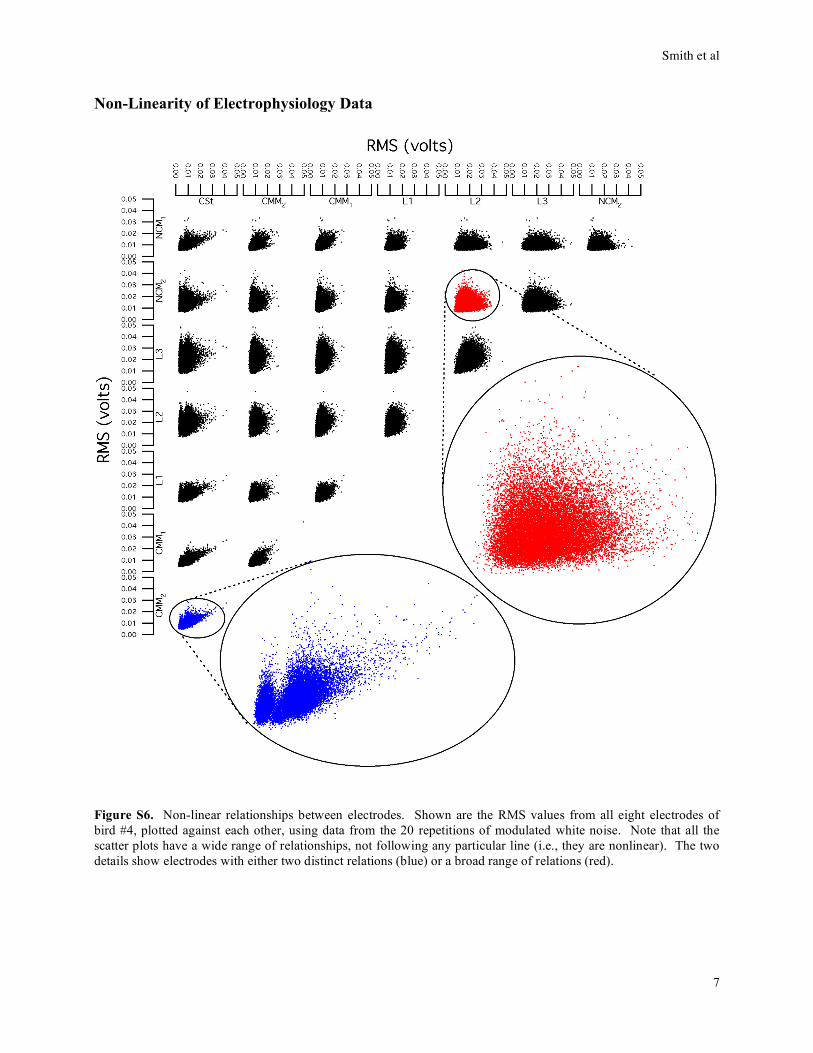
Non-Linearity of Electrophysiology Data

Figure S6. Non-linear relationships between electrodes. Shown are the RMS values from all eight electrodes of

bird #4, plotted against each other, using data from the 20 repetitions of modulated white noise. Note that all the

scatter plots have a wide range of relationships, not following any particular line (i.e., they are nonlinear). The two

details show electrodes with either two distinct relations (blue) or a broad range of relations (red).

Smith et al

8

SUPPORTING METHODS: Protocol S1, Figures S7 and S8

Electrophysiology Experiments

i) Electrode arrays and surgery

To a nine-channel nano-connector (Omnetics Corp., Minneapolis, MN), we attached 8

blunt-cut isonel-insulated tungsten microwire electrodes (50 μm diameter; impedance

approximately 0.8 Mohms, range: 0.6-1.2). The electrodes were positioned in a straight line.

The rostral-most electrode (electrode 1) was situated ~375 μm in front of the next electrode

(electrode 2), followed by others each spaced ~250 μm apart. The electrodes were cut in such a

way that electrode 1 was the longest and electrodes 2-8 were the shortest to the next longest, at an

angle of 30º from the horizontal (Fig. S1b). This configuration ensured that during surgery

electrode 1 was aimed at CSt, while the other seven covered the stretch from CMM through L1,

L2, L3, to NCM. A ninth electrode was added either behind electrode 8 or in front of electrode 1

as a ground (with a large section of insulation removed; in birds 1-4) or as a reference electrode

(similar to the other electrodes, but implanted in a non-auditory brain region anterior to CMM; in

birds 5 and 6). In the latter case, a separate silver wire was used as the ground electrode. This

set-up (with separate reference and ground electrodes) significantly reduced the amount of

movement artifact.

Before implant, fluorescent DiI (red) and DiO (yellow) dyes (Molecular Probes, Eugene,

OR) were applied and dried to alternating electrode tips in the array, such that their locations in

the brain could later be identified. The dyes did not interfere with the electrode recordings nor

with the types of responses the neurons gave when compared to a control implant that had

electrodes without dyes (see also [1,2]). The arrays were implanted under isoflurane anesthesia.

Birds were fixed in a custom-made stereotaxic frame (H. Adams, CalTech) with the head held at

a 45o angle. On one side of the brain, a rectangular opening was made in the skull above the

auditory areas and the array was lined up parallel to the midline of the brain. Electrode 1 was

zeroed to the split in the mid-sagittal sinus (visible through the bottom layer of the skull),

maneuvered 2.75mm rostral, 0.45-0.7 mm lateral (slightly different coordinates in different

birds), and then lowered to ~2.7mm below the surface, with the other electrodes following in

their pre-configured positions. Every time an electrode almost touched the dura mater, a small

slit was cut into the dura to allow the electrode to slip in. As the electrode array was advanced,

Smith et al

9

electrophysiological activity on each electrode was recorded using an extracellular amplifier

(FHC Inc, Bowdoinham, ME) and custom-written software in LabView™ 6.1 (National

Instruments, Austin, TX). The LabView software was based upon that developed in the

laboratory of R. Mooney (version of F. Livingstone and M. Rosen). To search for auditory

responses, the experimenter whistled scales. When at a depth where all or most of the electrodes

showed increased multi-unit responses to the whistles, the array was left in place and attached to

the skull using dental cement and cyanoacrylate glue. The birds were allowed to wake up and

were eating and drinking within 20 minutes. After ~2 days of recovery, they were attached to the

recording set-up in a soundproofed anechoic room in a 43 x 60 cm cage.

We chose this stable chronic set-up to obtain multi-unit recordings, instead of a

microdrivable one to obtain single units, as we considered anatomical stability across days to be

more important. This way, we ascertain the response properties of the same small populations of

neurons to a wide range of stimuli, in awake, behaving birds. This would have been impossible

with single unit recordings, which would either have required restrained or anaesthetized birds, or

would only have allowed recording from the same electrode for short amounts of time (< 1 hour

typically). Multi-unit changes are interpreted either as changes in the population response by all

individual neurons making up the population responding in the same way or by subsets of

neurons changing their response.

All experiments were approved by the Duke University Institutional Animal Care and Use

Committee.

ii) Electrophysiological recordings

The recording room was separated from an anteroom, in which the experimenter was

located together with all the recording equipment, by a one-way window. Through this window

and a TV monitor in the recording room connected to a SONY DCR-PC100 Digital HandyCam,

the bird’s behavior was monitored. The birds had ad lib food and water in the cage and the lights

were set to a 12/12 L/D schedule. We recorded multi-unit activity through a lightweight

recording cable with headstage (Plexon Inc, Dallas, TX), connected to the nano-connector

attached to the bird at one end (Fig. S1a), and a motorized commutator (Dragonfly Inc, Ridgeley,

WV) attached to the cage at the other end. This cable was connected at all times, and the birds

Smith et al

10

habituated to its presence overnight, after which the experiments were started. Once habituated,

the birds moved around freely in their cage, eating, drinking, flying, sleeping and grooming.

The headstage contained one unit-gain op-amp for each channel, including the reference

wire, to match the impedance of the wires to the impedance of the amplifier. The reference

channel was split into a non-amplified ground channel and an amplified reference channel for

birds 1-4, whereas for birds 5 and 6 the connection between ground and reference was cut to

reduce movement artifact and a separate groundwire was implanted. The signals from the

commutator were sent to a multi-channel extracellular amplifier (500x amplification, band-pass

filtered between 220 Hz and 5.9 kHz; Plexon, Inc., Houston, TX) and from there on to a PCI-

6071E Analog to Digital conversion card (National Instruments, Austin, TX) in the computer.

The data were digitized at 20 kHz using our custom-written LabView software. We also

recorded the sound in the recording room using a Sennheiser ME62 microphone, amplified via a

Midiman microphone amplifier, fed into the PCI-6071E card, and digitized together with the

electrophysiological data, at the same rate.

iii) Anatomy

In the last recording session, the birds were exposed to 50 repetitions of a novel

conspecific song for 15 minutes to induce immediate early gene expression [3]. We then waited

another 10 minutes to let the mRNA accumulate before quickly decapitating the birds, dissecting

out the brain and fast-freezing it. Brains were stored at -80ºC until processing. Brains were cut

on a cryostat into four or six series of alternate 10 μm sagittal sections. One series was stained

with DAPI and coverslipped for examination of the alternating fluorescent DiI and DiO electrode

tracts. Another series was hybridized with radioactive RNA probe for the immediate early gene

egr-1 using a previously established procedure [4] to visualize known gene expression

differences in the auditory forebrain areas [5]. We identified L2 by its lower egr-1 levels relative

to the surrounding brain areas. Thus, we had four means of anatomically identifying electrode

locations: 1) fluorescent dye from the electrode tips; 2) hearing-induced egr-1 gene expression

patterns; 3) gliosis along the electrode tracts in some cases, and 4) known cresyl-violet defined

boundaries among brain regions. This ensured highly accurate location of recording sites. It also

allowed determination of relationships between neural activity and hearing-induced gene

expression, which will be reported separately.

Smith et al

11

Based upon their locations, all electrodes in all birds were found and assigned to one of

six auditory forebrain areas (Fig. S1c-e): NCM, Field L3, Field L2, Field L1, CMM, and CSt. To

assign the electrodes to these specific brain areas, we looked for the section that contained the

electrode tip (deepest point of the tract) and determined its location in the auditory forebrain

relative to the different laminae. Since the boundary between L3 and NCM is not easy to

determine in Nissl stain or with egr-1, we estimated it based on the distance from L2 (~0.4mm).

iv) Playbacks

During playbacks, the birds were able to move around freely. This advantage of having

more natural behavior came with some loss in control over the animal’s position relative to the

sound source. We compensated for this loss in several ways. Firstly, stimuli were played

simultaneously from 2 speakers located equidistantly on either side of the cage, placed as far as

possible from the cage (approximately 60 cm from the nearest point of the cage), so that any

movement of the bird would represent only a fraction of the distance between it and the speaker.

Movement away from one speaker would automatically bring the bird closer to the other speaker.

Turning the ear contralateral to the recording away from one speaker again would automatically

result in turning it towards the other one. Because of this set-up, the movements of the bird do

not result in significant changes in the stimulus intensity as they reach the ears of the birds.

Stimuli were encoded as WAV files. Each song stimulus consisted of two motifs, without

introductory notes. White noise and modulated white noise were generated using custom-written

software in LabView. All stimuli were preceded and followed by a period of silence of exactly

the same length as the stimulus itself. We generated similar intensities for all stimuli by playing

them through the same speakers as used in the experiment, re-recording them (digitized at 20

kHz) using a microphone with a flat spectral response profile (Radioshack lapel microphone),

and then adjusting the volume of the stimulus until all stimuli produced a microphone-recorded

signal with the same Root Mean Square (RMS), resulting in a similar average power across

stimuli. The speakers were Cambridge Soundworks Creative CSW1500 surround sound gaming

speakers connected to a SoundBlaster Live card in the computer and controlled through custom-

written software in LabView. The speaker level was set so that a 1 kHz pure tone delivered 80

dB SPL in the center of the cage (Radioshack dB meter).

Smith et al

12

Dynamic Bayesian Network (DBN) Inference Algorithm.

Details on the theory of Bayesian networks and DBNs can be found in Friedman et al. [6] and

Heckerman et al. [7]. The interested reader is also referred to Cowell 2001 [8], wherein is

described the mathematical equivalence of score-based and conditional independence test-based

methods of determining the best Bayesian network to model a data set. The specific software we

used was developed by Yu et al. [9] in C++, based upon earlier software developed by Hartemink

in C. We later developed a more flexible, efficient, and user-friendly software package in Java

called Banjo. Banjo can be licensed free for non-commercial use and is available with complete

source code over the web from http://www.cs.duke.edu/~amink/software/banjo/. The C++

research-grade version is available upon request. Each of the four elements in our algorithm

mentioned in the Methods section of the main text is described below in the context of neural

information flow networks.

i) DBN model

A DBN is an extension of a static Bayesian network (BN). A BN is a graphical representation of

a joint probability distribution over , where ={X1, ..., Xn} is a set of random variables Xi. A BN

is specified as a pair <G, >. The variable G represents a directed acyclic graph whose vertices

correspond to the random variables X1, ..., Xn (activity levels at one of the individual electrode

locations in our case) and whose directed links from Xi to Xj indicate a statistical conditional

dependence of Xj on Xi. All variables which have a directed link to Xi are known as its parents

[Pa(Xi)]; all variables to which Xi has a directed link, and recursively all variables receiving links

from such targeted variables and their targets, are known as its descendents. Each variable Xi is

independent of its non-descendents in G given its parents in G. The variable represents the

collection of parameters that quantify the probability distributions associated with each variable

Xi. Each of these probability distribution parameters is specified as x i | pa(Xi )=

P(Xi=xi|Pa(Xi)=pa(Xi)): namely, the probability of Xi taking on the value xi (one of the discretized

RMS values in our case) given its parents Pa(Xi) having the values in a particular instantiation of

the parents, pa(Xi), for all xi and pa(Xi). These parameters combine to form the unique joint

probability distribution:

P(X1, ..., Xn) = i=1

nP(Xi |Pa(Xi)).

Smith et al

13

Note that this probability distribution allows arbitrary combinatoric relationships between parent

and child values: each x i | pa(Xi ) is unique to its parent configuration and child state. This feature

allows discrete BNs to model many types of relationships, including nonlinear and nonadditive

relationships.

A DBN extends this framework by including the dimension of time. We use a first-order

Markov DBN, meaning that we consider variables at one time step to be affected only by those in

the immediately previous time step. Such a DBN is a graphical representation of a joint

probability distribution over ', where ' ={X1(t), ..., Xn(t), X1(t+ t), ..., Xn(t+ t)} is a set of discrete

random variables Xi measured at both time t and time t+ t ( t=5ms in our case). Just like a BN,

a DBN is specified as a pair <G, >. The graph G (an information flow network in our case) is

restricted in a DBN so that links are only allowed to go forward in time, i.e., from a variable Xi(t)

to Xj(t+ t). Additionally, we require that all variables must have directed links from themselves at

time t to themselves at time t+ t, i.e., all Xi(t) link to Xi(t+ t). The collection of parameters

consist of x i( t+ t ) | pa (X i ( t+ t ) ), as above, for all Xi(t+ t) in '.

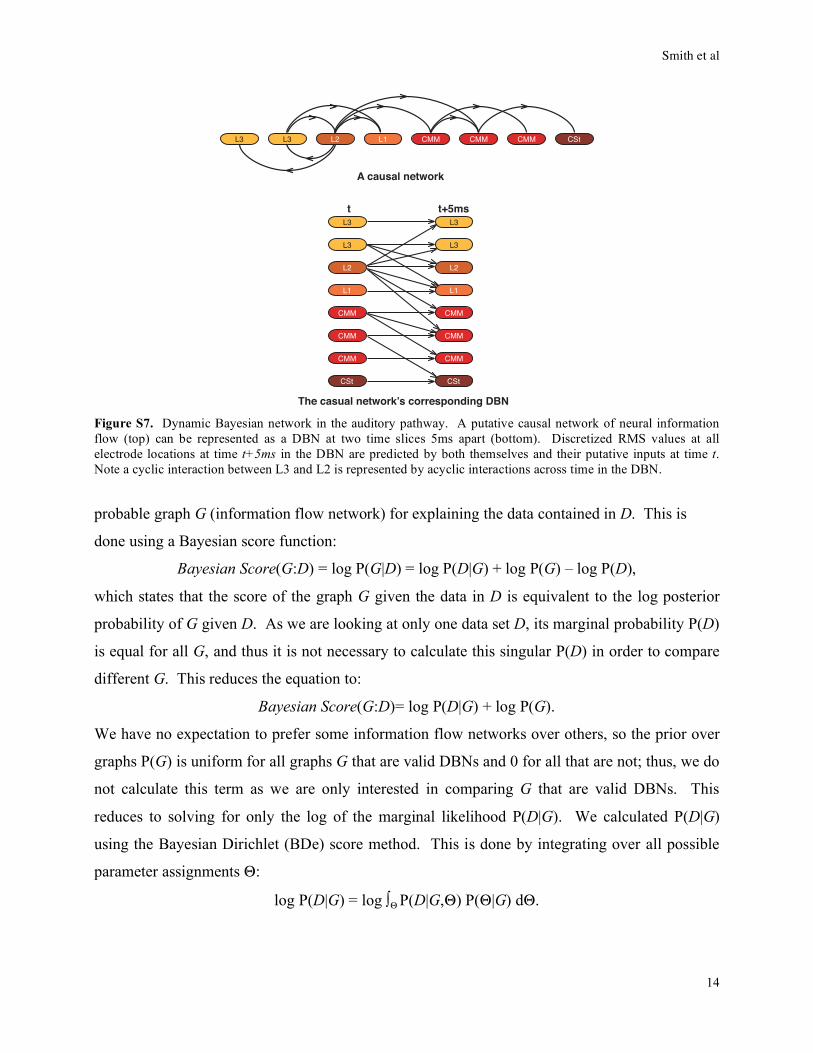
We used a DBN because it has two important advantages over static BNs to model

biological systems. First, BNs cannot model feedback loops among variables due to the

acyclicity restriction on the graph G. However, information flow in the brain can be reciprocal.

A DBN allows representation of cyclic interactions between two or more variables over time

because it models all variables at more than one point in time: a cycle over time is represented as

acyclic interactions between variables across the two times (Fig. S7). Second, the unique joint

probability distribution of a BN can sometimes have several different equivalent factorings that

differ only in the direction of some links. These graphs form a Markov equivalence class and are

indistinguishable probabilistically, leading to uncertainty about the direction of influence

between variables. In contrast, in a DBN only one factoring in the Markov equivalence class will

match the additional restriction that the direction of links in G go forward in time, as is expected

with brain function, and thus there is no uncertainty about direction of influence.

ii) Bayesian scoring metric

The problem of discovering a DBN (or BN) from a collection of observed data is stated as: Given

a data set D={Y1, ..., Ym} of observed instances of , where Yk represents a vector of values

(discretized RMS values in our case) for each Xi (electrode location) in at time k, find the most

Smith et al

14

L3

L3

L2

L1

CMM

CMM

CMM

CSt

L3

L3

L2

L1

CMM

CMM

CMM

CSt

t t+5ms

CStL1L3 L3 CMMCMMCMML2

A causal network

The casual network’s corresponding DBN

Figure S7. Dynamic Bayesian network in the auditory pathway. A putative causal network of neural information

flow (top) can be represented as a DBN at two time slices 5ms apart (bottom). Discretized RMS values at all

electrode locations at time t+5ms in the DBN are predicted by both themselves and their putative inputs at time t.

Note a cyclic interaction between L3 and L2 is represented by acyclic interactions across time in the DBN.

probable graph G (information flow network) for explaining the data contained in D. This is

done using a Bayesian score function:

Bayesian Score(G:D) = log P(G|D) = log P(D|G) + log P(G) – log P(D),

which states that the score of the graph G given the data in D is equivalent to the log posterior

probability of G given D. As we are looking at only one data set D, its marginal probability P(D)

is equal for all G, and thus it is not necessary to calculate this singular P(D) in order to compare

different G. This reduces the equation to:

Bayesian Score(G:D)= log P(D|G) + log P(G).

We have no expectation to prefer some information flow networks over others, so the prior over

graphs P(G) is uniform for all graphs G that are valid DBNs and 0 for all that are not; thus, we do

not calculate this term as we are only interested in comparing G that are valid DBNs. This

reduces to solving for only the log of the marginal likelihood P(D|G). We calculated P(D|G)

using the Bayesian Dirichlet (BDe) score method. This is done by integrating over all possible

parameter assignments :

log P(D|G) = log P(D|G, ) P( |G) d .

Smith et al

15

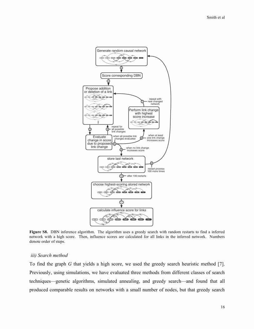
This integral is solvable, assuming the prior over parameters P( |G) is Dirichlet (the conjugate

distribution for a multinomial), as:

log P(D|G)= log (( ij )

( ij + Nij )

( ijk + Nijk )

( ijk)k=1

ri

j= i

qi

i=1

n),

where n is the number of variables Xi in , qi is the number of parent instantiations pa(Xi) of the

parents of Xi, ri is the number of values xi of Xi, (·) is the gamma function, ij and ijk are

equivalent sample size statistics of the Dirichlet prior distribution, and Nij and Nijk are counts in D

of the number of times the parents of Xi take on instantiation j, and the number of times the

variable Xi takes on value k with parents in instantiation j, respectively.

To provide an intuitive understanding how this score relates to the data, we note the

following: The rightmost product term, ( ijk+ Nijk)/ ( ijk), is higher when the counts are more

concentrated in a particular child value. This indicates that the scores are better when a given

parent state is more useful for predicting the child, matching with the definition of statistical

dependence. The other product term, ( ij)/ ( ij + Nij), is higher with (a) fewer parent states and

(b) equal examples of each state. The feature (a) is the inherent penalty for complexity which

prevents over-fitting of the data, and the feature (b) indicates that the score is higher when the

data is distributed more evenly across its possible values.

In addition to the actual data, two other factors influence this score: the value used for the

Diriichlet prior's equivalent sample size (ess) and the level of discretization of the variables. The

effect of the ess is such that a higher value means the prior belief is more strongly that ‘anything

can happen’: the score for any interaction is higher and thus it is easier for any link to be found.

We used a low ess of 1 to put a large emphasis on the influence of the data for determining which

links exist. The effect of discretization is such that more discrete levels can lead to more detailed

predictive power from parent state to child state, but it also leads to more parent states and more

sensitivity to noise. Because we discretize using a quantile method, it does not lead to more

unevenly distributed data across states, although with other discretization methods this could be

the case. Since these features affect inference accuracy in opposing ways, we must find a balance

between using more discrete levels to capture more detail and fewer to give us statistical power to

find those relationships that exist. We have found using simulation studies that three-level

discretization works well with our algorithm [9], and used this here.

Smith et al

16

when all possible linkchanges evaluated

when no link change increases score

after 100 restarts

store last network


choose highest-scoring stored network


calculate influence score for links

CSt

0.40

0.26

0.19

0.19

0.24

0.18

0.16

0.09 0.10

L1L3 L3 CMMCMMCMML2

0.24

restart process100 more times

Perform link changewith highest

score increaseCStL3 L3 L2 L1 CMM CMM CMM

Generate random causal network

CStL3 L3 L2 L1 CMM CMM CMM

Score corresponding DBN

repeat forall possiblelink changes

Propose additionor deletion of a link




Evaluatechange in scoredue to proposed

link change

1

2

3 4

5

6

8

7

9

10

11

when at leastone link changeincreases score

repeat withnew changed

network

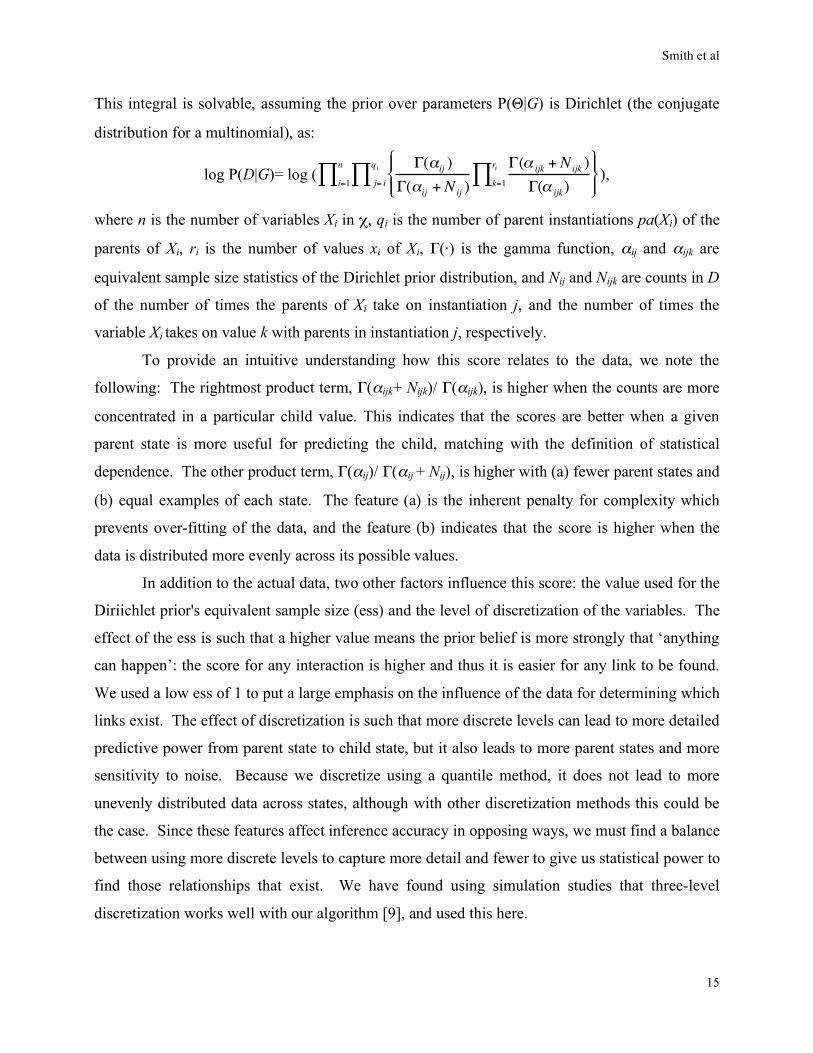
Figure S8. DBN inference algorithm. The algorithm uses a greedy search with random restarts to find a inferred

network with a high score. Then, influence scores are calculated for all links in the inferred network. Numbers

denote order of steps.

iii) Search method

To find the graph G that yields a high score, we used the greedy search heuristic method [7].

Previously, using simulations, we have evaluated three methods from different classes of search

techniques—genetic algorithms, simulated annealing, and greedy search—and found that all

produced comparable results on networks with a small number of nodes, but that greedy search

Smith et al

17

was the fastest computationally [9]. A greedy search begins with a randomly chosen initial

graph. To this graph, addition or deletion of links are evaluated, and the change with the greatest

score increase is performed. This process is repeated iteratively until no change improves the

score. To escape from local maxima, the search restarts again with a new initial random graph.

We used 100 such restarts, and chose the graph with the highest score as the inferred network

(Fig. S8). Overall, this process searches approximately 10 million distinct graphs before

choosing the inferred network.

iv) Influence score

The influence score we developed for DBN algorithms is described in detail elsewhere [9]; the

most precise statement of its calculation can be found in the code for the Banjo software which

implements it (freely available at http://www.cs.duke.edu/~amink/software/banjo/). Briefly, it is

a summarization of the conditional probability relationships in a Bayesian network to

approximate the sign (excitatory or inhibitory in our case) and magnitude of the interaction

between a variable and each of its parents (inputs). This is based on the intuition that if a variable

tends to have a high value when its parent is high and a low value when its parent is low, the

parent is presumably an activator; conversely, if a variable tends to have a low value when its

parent is high and a high value when its parent is low, the parent is presumably a repressor. We

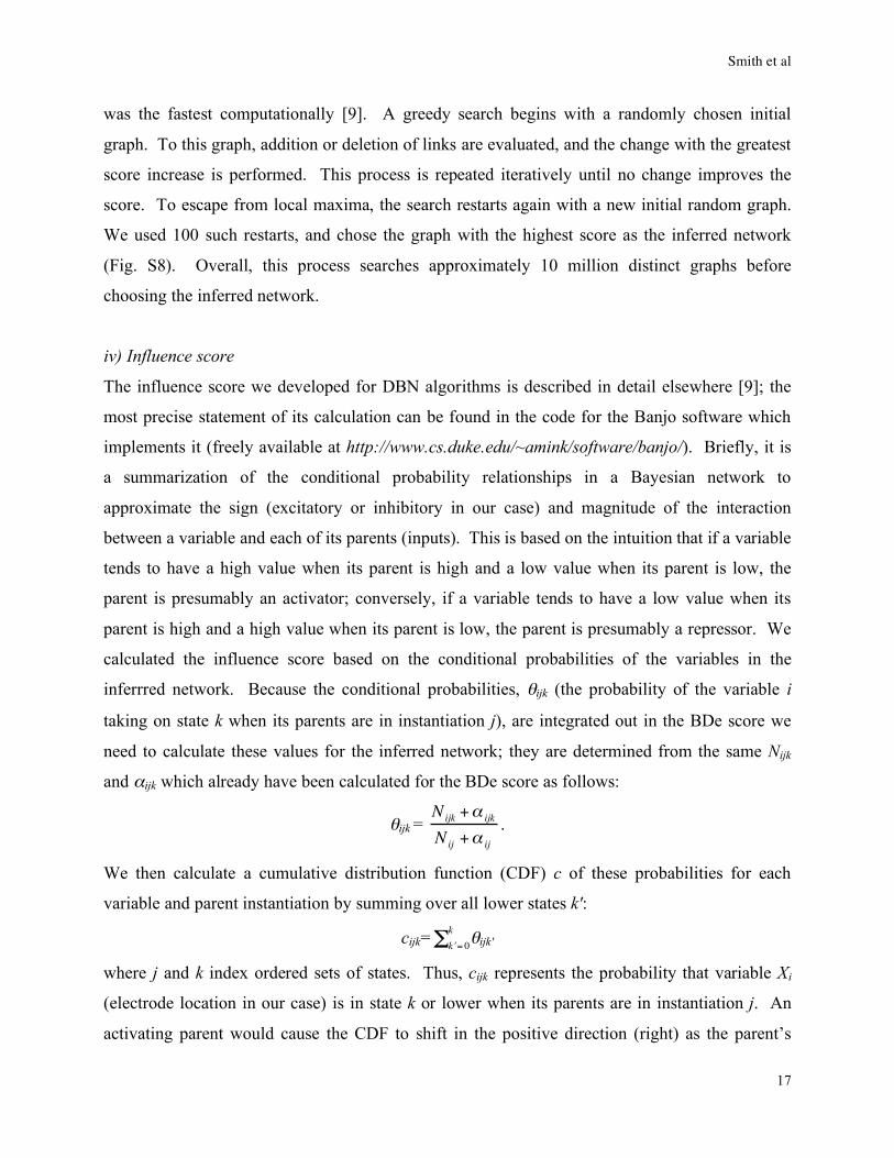
calculated the influence score based on the conditional probabilities of the variables in the

inferrred network. Because the conditional probabilities, ijk (the probability of the variable i

taking on state k when its parents are in instantiation j), are integrated out in the BDe score we

need to calculate these values for the inferred network; they are determined from the same Nijk

and ijk which already have been calculated for the BDe score as follows:

ijk = Nijk + ijk

Nij + ij

.

We then calculate a cumulative distribution function (CDF) c of these probabilities for each

variable and parent instantiation by summing over all lower states k':

cijk= k = 0

kijk'

where j and k index ordered sets of states. Thus, cijk represents the probability that variable Xi

(electrode location in our case) is in state k or lower when its parents are in instantiation j. An

activating parent would cause the CDF to shift in the positive direction (right) as the parent’s

Smith et al

18

value increases; vice versa for repressing parents. We pass these cijk values through a voting

system. Each parent gets one vote for each of the possible configurations of the other parents,

e.g., with three parents each having three states, each parent votes nine times for the nine (3*3)

possible configurations of the other parents. Voting occurs with the other parents held constant

in one of their states, and is based on a comparison of an ordered array of cijk’s such that j-1

indexes the parent state for which the parent in question has a value of one ordered state less than

it does in state j. If all cijk ci(j-1)k (CDF shift positive), the vote is for a positive interaction; if all

cijk ci(j-1)k (CDF shift negative), the vote is for a negative interaction; if neither of these hold, the

vote is neutral. If all of a parent’s votes are positive or positive and neutral, it is considered an

activator and the sign of the influence score is set to be positive (+); if all of a parent’s votes are

negative or negative and neutral, it is considered a repressor and the sign of the influence score is

set to be negative (–); if the votes are both positive and negative, the sign is indeterminate and the

influence score is set to 0. Otherwise, the magnitude of the influence score is equal to the sum of

the non-neutral votes of the difference between cij'k and cij''k, where j' and j'' are the parent

instantiations when this parent is at its lowest and highest values, respectively. The score is then

divided by the total number of votes (including neutral) to scale it between –1 to 1. The greater

the magnitude of the influence score, the more strongly the parent is an activator or repressor (or

in our case, the stronger the net positive or negative interaction between brain regions).

Technical Note

We note that while the networks we infer are referred to as ‘neural information flow networks’,

this terminology does not refer directly to ‘information’ in the information theoretic sense—it is

instead a descriptive term used within neuroscience.

Smith et al

19

REFERENCES

1. DiCarlo JJ, Lane JW, Hsiao SS, Johnson KO (1996) Marking microelectrode penetrations with

fluorescent dyes. J Neurosci Methods 64: 75-81.

2. Naselaris T, Merchant H, Amirikian B, Georgopoulos AP (2005) Spatial reconstruction of

trajectories of an array of recording microelectrodes. J Neurophysiol 93: 2318-2330.

3. Mello CV, Nottebohm F, Clayton D (1995) Repeated exposure to one song leads to a rapid and

persistent decline in an immediate early gene's response to that song in zebra finch

telencephalon. J Neurosci 15: 6919-6925.

4. Jarvis ED, Nottebohm F (1997) Motor-driven gene expression. Proc Natl Acad Sci U S A 94:

4097-4102.

5. Mello CV, Clayton DF (1994) Song-induced ZENK gene expression in auditory pathways of

songbird brain and its relation to the song control system. J Neurosci 14: 6652-6666.

6. Friedman N, Murphy K, Russell S (1998) Learning the structure of dynamic probabilistic

networks. Proceedings of the Fourteenth Conference on Uncertainty in Artificial

Intelligence. San Francisco, CA: Morgan Kaufmann. pp. 139-147.

7. Heckerman D, Geiger D, Chickering DM (1995) Learning Bayesian networks: The

combination of knowledge and statistical data. Mach Learn 20: 197-243.

8. Cowell RG (2001) Conditions under which conditional independence and scoring methods

lead to identical selection of Bayesian network models. Proceedings of the 17th

Conference in Uncertainty in Artificial Intelligence. San Francisco: Morgan Kaufmann

Publishers Inc. pp. 91-97.

9. Yu J, Smith VA, Wang PP, Hartemink AJ, Jarvis ED (2004) Advances to Bayesian network

inference for generating causal networks from observational biological data.

Bioinformatics 20: 3594-3603.

Documents

SUPPORTING RESULTS: Figures S1-S6, Tables S1-S3amink/publications/manuscripts/... · Smith et al 8 SUPPORTING METHODS: Protocol S1, Figures S7 and S8 Electrophysiology Experiments