Supplementary Materials for

Has land use pushed terrestrial biodiversity beyond the planetary boundary? A global assessment

Tim Newbold1,2,*, Lawrence N. Hudson3, Andrew P. Arnell1, Sara Contu3, Adriana De Palma3,4, Simon Ferrier5, Samantha L. L. Hill1,3, Andrew J. Hoskins5, Igor Lysenko4,

Helen R. P. Phillips3,4, Victoria J. Burton3, Charlotte W.T. Chng3, Susan Emerson3, Di Gao3, Gwilym Pask-Hale3, Jon Hutton1,6, Martin Jung7,8, Katia Sanchez-Ortiz3, Benno I. Simmons3, Sarah Whitmee2, Hanbin Zhang3, Jörn P.W. Scharlemann8, Andy Purvis3,4

correspondence to: t.newbold@ucl.ac.uk

This PDF file includes:

Materials and MethodsFigs. S1 to S7Tables S1 to S7

1

12

1

2

3

45

6

7

89

10111213141516171819202122

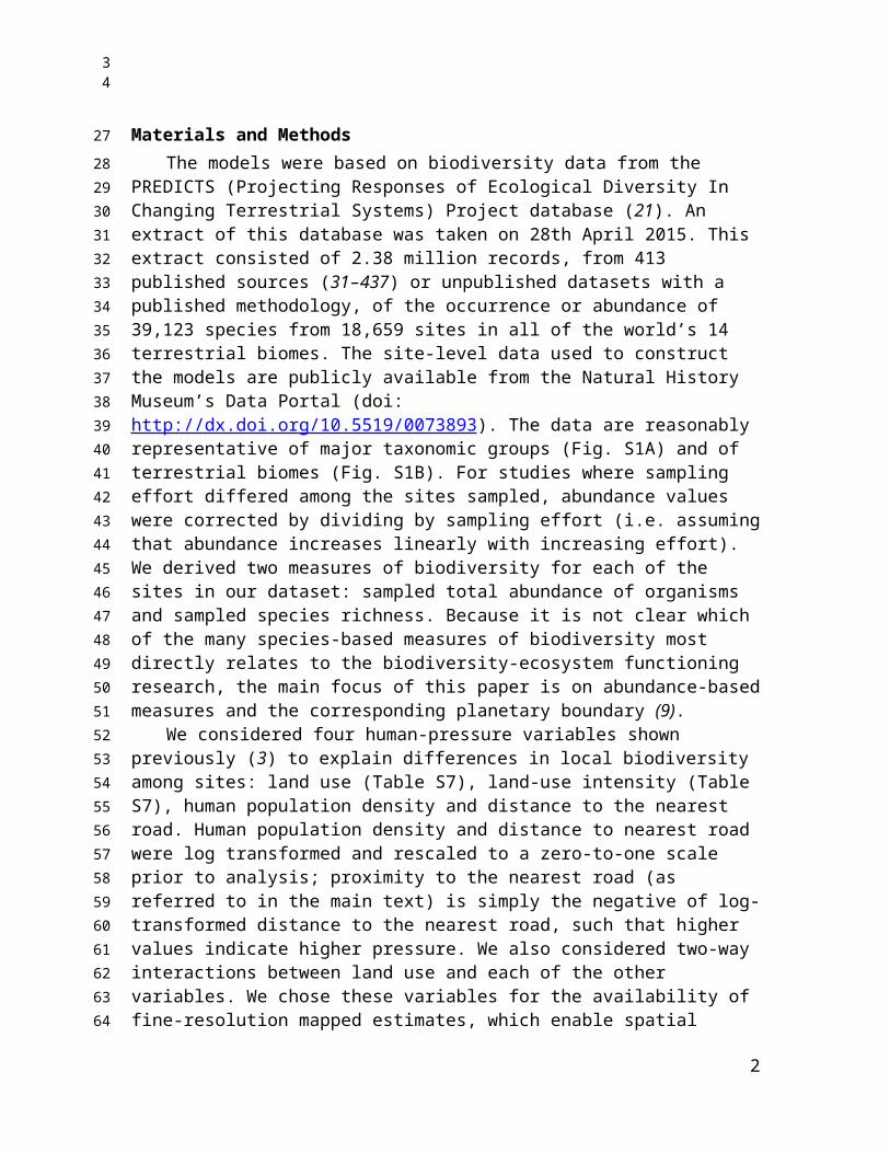
Materials and MethodsThe models were based on biodiversity data from the PREDICTS (Projecting

Responses of Ecological Diversity In Changing Terrestrial Systems) Project database (21). An extract of this database was taken on 28th April 2015. This extract consisted of 2.38 million records, from 413 published sources (31–437) or unpublished datasets with a published methodology, of the occurrence or abundance of 39,123 species from 18,659 sites in all of the world’s 14 terrestrial biomes. The site-level data used to construct the models are publicly available from the Natural History Museum’s Data Portal (doi: http://dx.doi.org/10.5519/0073893). The data are reasonably representative of major taxonomic groups (Fig. S1A) and of terrestrial biomes (Fig. S1B). For studies where sampling effort differed among the sites sampled, abundance values were corrected by dividing by sampling effort (i.e. assuming that abundance increases linearly with increasing effort). We derived two measures of biodiversity for each of the sites in our dataset: sampled total abundance of organisms and sampled species richness. Because it is not clear which of the many species-based measures of biodiversity most directly relates to the biodiversity-ecosystem functioning research, the main focus of this paper is on abundance-based measures and the corresponding planetary boundary (9).

We considered four human-pressure variables shown previously (3) to explain differences in local biodiversity among sites: land use (Table S7), land-use intensity (Table S7), human population density and distance to the nearest road. Human population density and distance to nearest road were log transformed and rescaled to a zero-to-one scale prior to analysis; proximity to the nearest road (as referred to in the main text) is simply the negative of log-transformed distance to the nearest road, such that higher values indicate higher pressure. We also considered two-way interactions between land use and each of the other variables. We chose these variables for the availability of fine-resolution mapped estimates, which enable spatial projections to be made from the models. Responses of biodiversity to these variables were modelled using generalized linear mixed-effects models. For sampled species richness we used a model with Poisson errors and a log link, while for (log-transformed) sampled total abundance we used a model with Gaussian errors and an identity link. A random effect of study identity was used to account for variation among studies in sampling methods and effort, differences in the taxonomic groups sampled, and coarse spatial differences in climate and other aspects of the environment. A random effect of spatial block nested within study, to take account of the spatial design of sampling. Spatial blocks were defined by the data entrants based on the maps and coordinates of sampled sites. A random slope of land use within study accounted for study-level variation in the relationship between land use and sampled biodiversity. Backward stepwise selection of fixed effects was used to select the minimum adequate model (438), with inclusion or exclusion of terms based on likelihood ratio tests (with a threshold P < 0.05). All models were developed using the lme4 Version 1.1-7 package (439) in R Version 3.2.2 (440). Spatial autocorrelation tests, performed as in (3), showed significant spatial autocorrelation in the model residuals for only slightly more of the modelled datasets than expected by chance: 6.1% in the case of species richness, and 5.9% in the case of total abundance.

To project mapped estimates of local biodiversity in the year 2005, we used fine-resolution maps of each of the four human pressure variables. The maps of land use were

2

34

24

2526272829303132333435363738394041424344454647484950515253545556575859606162636465666768

generated by downscaling (23) the harmonized land-use dataset for 2005 (441). The harmonized land-use data describe the proportion of each 0.5° (approximately 50 km2) grid cell in each of five land uses (primary vegetation, secondary vegetation, cropland, pasture and urban). We used generalized additive models (GAM) with quasibinomial errors and a logistic link to relate coarse-scale estimates of each of the five land uses to nine putative explanatory variables at fine resolution (30 arc-seconds; approximately 1 km2): evapotranspiration (442), temperature (443), precipitation (443), topographic wetness (444), slope (444), soil carbon (445), accessibility to humans (446), human population density (24) and principal components of land cover (447). We then took the fine-grained fitted values from the GAMs and rescaled them multiplicatively until the aggregated mean for each 0.5° grid cell matched the estimates from the harmonized land-use data. The rescaled fitted values were then subjected to a constrained optimization algorithm, taking into account error estimates from the GAMs, to generate land-use estimates for all five land uses that summed to 1 within each grid cell. We entered the final estimates back into the GAMs as response variables, and the whole procedure was iterated until the mean inter-iteration difference of predicted values was ≤ 0.001. Grid cells under ice or water (448, 449) were excluded from the analysis, and were masked from the final land-use maps. For full details on downscaling methodology see (23). The land-use data are freely available: http://doi.org/10.4225/08/56DCD9249B224.

In a previous study (3), to estimate spatial patterns of land-use intensity, we used generalized linear models (with binomial errors and a logistic link), for each level of intensity within each land use, to relate the proportion of each 0.5° grid cell under this combination of land use and intensity to three explanatory variables: the proportion of the cell under the land use in question, human population density and United Nations sub-region. Information on land-use intensity was obtained from the Global Land Systems dataset (450); see (3) for the reclassification used. To run these generalized linear models for every 30-arc-second grid cell was computationally infeasible. Therefore, we applied the coarse-resolution models developed for the previous study (3) at the fine resolution used here, assuming that the relationships are the same at both scales. We obtained a gridded map of human population density at 30-arc-second resolution and a vector map of the world’s roads from NASA’s Socioeconomic Data and Applications Centre (24, 25). To calculate a gridded map of distance to nearest road, we used Python code written for the arcpy module of ArcMap Version 10.3 (451), first to project the vector map of roads onto an equal-area (Behrmann) projection, then to calculate the average distance to the nearest road within each 782-m grid cell using the ‘Euclidean Distance’ function, and finally to reproject the resulting map back to a WGS 1984 projection at 30-arc-second resolution. Maximum estimated values across the terrestrial surface of human population density and distance to nearest road in 2005 were 8.3% and 20% higher, respectively, than the maximum values observed in the modelled dataset. To ensure that extrapolating did not create unrealistic projections, we set all grid cells with values higher than the maximum observed to be equal to this maximum observed value (this affected 0.002% of grid cells for human population density and 5.6% of grid cells for distance to nearest road). We could not estimate the expected species richness with absolutely no influence of roads because it is impossible to collect a sample of biodiversity under such a situation in the present day.

3

56

69707172737475767778798081828384858687888990919293949596979899

100101102103104105106107108109110111112113

To generate estimates of the intactness of ecological assemblages in terms of within-sample species richness and abundance, we multiplied the coefficients of the minimum adequate models described above by the proportion of each grid cell under each land-use and use-intensity combination, and by log-transformed and rescaled (using the same rescaling as in the models) human population density or distance to nearest road. We assumed that human population density and distance to nearest road were constant within grid cells. The resulting values were summed across all coefficients and the intercept added to give the model estimate of log-transformed species richness or total abundance within each grid cell. We calculated the exponential of these values to estimate actual species richness and total abundance. Finally, to calculate the relative intactness of assemblages relative to a baseline with no human impacts, we calculated expected species richness and total abundance for a grid cell composed entirely of primary vegetation with minimal human use, with zero human population density, and at a distance to roads equal to the maximum value observed in the modelling data (195 km). Estimating uncertainty analytically for mixed-effects models requires generating an n-by-n matrix, where n is the number of grid cells in the projection; this was computationally intractable. Instead we generated 20 random draws (a greater number would have required a long computer run-time) of values for all of the model coefficients, from a multivariate normal distribution accounting for the covariance among modelled coefficients. These random draws of parameters were used to generate 20 replicate projections, from which 95% confidence limits were calculated for each analysis. All of the calculations described in this paragraph were undertaken using Python code implemented within the arcpy module of ArcMap Version 10.3 (451), using the ‘Raster Calculator’ function; except for the multivariate random draw of coefficient values, which was performed in R Version 3.2.2 using the 'mvrnorm' function in the MASS package Version 7.3-43.

Scholes & Biggs (11) explicitly exclude alien species from the calculation of biodiversity intactness. Because it is not generally known which species are native and which not, we use modelled average compositional similarity between sites in primary vegetation and sites under other land uses as a multiplier on our land-use coefficients (on a 0-1 scale, rescaled such that primary-primary comparisons have a value of 1). To generate these modelled estimates of compositional similarity, we calculated asymmetric pairwise assemblage similarities between all possible pairs of sites within each study in the data set, where one site in the pair was in primary vegetation. Primary vegetation may contain species that are not truly native to an area, especially in landscapes with a long history of human modification; and landscape-level effects of land-use change may have already removed some originally-present species even from sites in primary vegetation. Therefore, our estimates of compositional similarity are likely to be biased upwards. Asymmetric values were used to focus on the probability that a species sampled in non-primary vegetation was also found in primary vegetation. To remove the possibility for pseudo-replication, we selected as independent contrasts all site comparisons on the off-diagonal of a randomized site-by-site matrix (452). Site-by-site matrices were randomised 100 times to generate 100 datasets of independent comparisons. Compositional similarity was measured using an asymmetric version of the Jaccard Index (J) for the projections of species richness, and an asymmetric version of the abundance-based Jaccard Index (Ja) (453) for the projections of total abundance:

4

78

114115116117118119120121122123124125126127128129130131132133134135136137138139140141142143144145146147148149150151152153154155156157158159

J= aa+c

Ja=UVV

where a is the number of species shared between the two sampled sites, c is the number of species only found in the site not in primary vegetation, U is the summed relative abundance in the primary-vegetation site of all species found in both sites, and V is the summed relative abundance in the non-primary site of all species found in both sites.

Assemblage compositional similarities in each of the 100 datasets were modelled as a function of the combination of land uses represented and the distance (geographic, climatic and elevational) between sites. Full details of how assemblage compositional similarity was modelled are given in (22). Average coefficients across the 100 models describing average compositional similarity between primary vegetation and all other land uses (including primary vegetation itself) were rescaled so that comparisons of primary vegetation to itself had a value of 1 (to avoid conflating natural spatial turnover with land-use impact). These rescaled coefficients were then multiplied by the modelled coefficients describing differences in species richness and total abundance among land uses, to estimate the number of species or individuals present in each land use that are also expected to be present in primary vegetation. The rescaled coefficients are publicly available from the Natural History Museum’s Data Portal (doi: http://dx.doi.org/10.5519/0073893).

Although our way of calculating BII differs from that proposed by Scholes & Biggs (11), we also attempt to estimate the “average abundance of a large and diverse set of organisms in an area, relative to their reference populations” (11). If Iijk is the population of species group i in ecosystem j under land use k, relative to a pre-industrial population in the same ecosystem type, then Scholes & Biggs (11) define the biodiversity intactness index (BII) to be:

BII = 100 x (ΣiΣjΣkRijAjkIijk) / (ΣiΣjΣkRijAjk)

where Rij is the species richness of taxon i in ecosystem j and Ajk is the area of ecosystem j under land use k. Scholes & Biggs (11) used expert opinion when estimating average BII for seven southern African countries, in the absence of sufficient primary data. They considered birds, mammals, amphibians, reptiles and angiosperms but not arthropods, again because of a lack of information.

Our implementation of the BII differs in that we have used primary data on sampled local species abundance – for a wide range of animal (vertebrates and invertebrates), plant and fungal taxa – in place of expert opinion, and our statistical models incorporate other pressures as well as land use itself. Rather than weighting by areas of ecosystems and species-richness of taxa, we have collated and analysed a data set that is reasonably representative in terms of biomes (Fig. S1B) and taxa (Fig. S1A). Our data set is not yet adequate to support fitting models for each biome and taxon separately, which may lead

5

910

160

161

162

163

164165166167168169170171172173174175176177178179180181182183184185186187188189190191192193194195196197198199200201202203

to our estimates being biased for some biomes. Despite our very large number of records, hierarchical mixed-effects models for individual biomes or taxa would require data from a larger number of published studies than is available for some taxa and biomes. As in (11), in the absence of pre-industrial data, we have used minimally-impacted sites as the reference condition.

We overlaid our estimates of the intactness of ecological assemblages with global maps describing the distribution of biomes (449), Conservation International’s biodiversity hotspots (28), Conservation International’s High Biodiversity Wilderness Areas (454) and human population density (24). All of these overlays were performed using Python code for ArcMap Version 10.3 (451), using the ‘Zonal Statistics’ functions after first projecting all maps into an equal-area (Behrmann) projection.

6

1112

204205206207208209210211212213214215

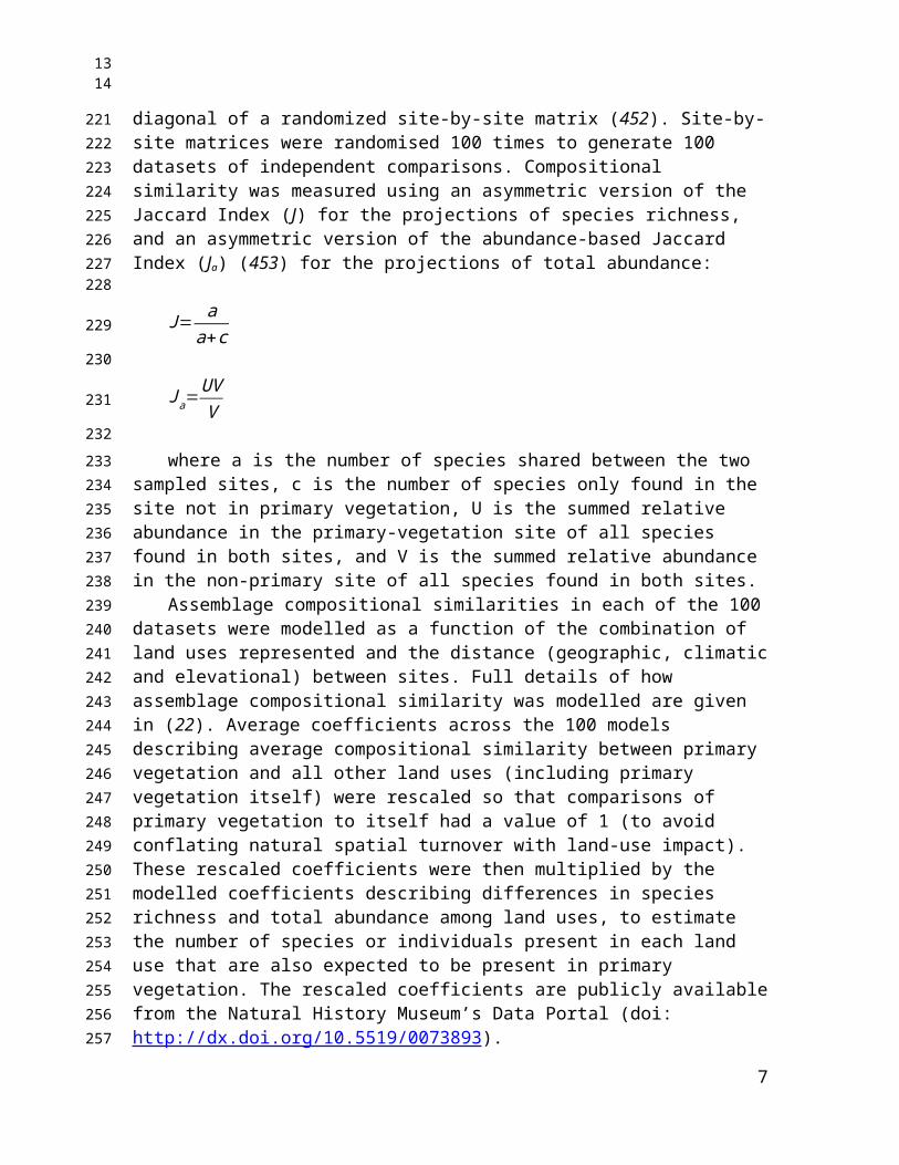
Fig. S1.

Fig. S1. Taxonomic (A) and biogeographic (B) representativeness of the records used to model biodiversity responses to land use. (A) Correlation, for major taxonomic groups (magenta ‒ invertebrates; red‒ vertebrates; green ‒ plants and fungi; grey ‒ other), between the estimated number of described species (455) and the number of species represented in the dataset. (B) Correlation between the percentage of global primary productivity within a biome (449) and the percentage of sites in the dataset within that biome (A: Tundra; B: Boreal forests/taiga; C: Temperate conifer forests; D: Temperate broadleaf and mixed forests; E: Montane grasslands and shrublands; F: Temperate grasslands, savannas and shrublands; G: Mediterranean forests, woodland and scrub; H: Deserts and xeric shrublands; J: Tropical and subtropical grasslands, savannas and shrublands; K: Tropical and subtropical coniferous forests; L: Flooded grasslands and savannas; M: Tropical and subtropical dry broadleaf forests; N: Tropical and subtropical moist broadleaf forests; P: Mangroves).

7

1314

216

217218219220221222223224225226227228229230231

Fig. S2

Fig. S2. Response of sampled total abundance to human pressures: (A) land use, and (B) the interaction between land use and human population density. Human population is shown on a rescaled axis (as fitted in the models). (A) shows total abundance as a percentage of that found in minimally used primary vegetation, with 95% confidence intervals; multiple points within each land-use type show, from left to right, increasing intensity of human use (two classes for secondary vegetation and urban; three classes for all other land uses). B shows absolute mean total abundance for a given combination of pressures, with shading indicating ±0.5 × SEM, for clarity. Land uses in B are shown in the same colours as in A. Mixed-effects models are robust to unbalanced designs (456), such as the data spanning different ranges of human population density for each of the land uses. Dropping all urban sites almost no effect on the other model coefficients (Fig. S6). Full statistical results are given in Table S5.

8

1516

232

233

234235236237238239240241242243244245246247

Fig. S3

Fig. S3. Response of sampled species richness to human pressures: (A) land use, (B) the interaction between land use and human population density, and (C) the interaction between land use and distance to nearest road. Human population and distance to nearest road are shown on rescaled axes (as fitted in the models). (A) shows species richness as a percentage of that found in minimally used primary vegetation, with 95% confidence intervals; multiple points within each land-use type show, from left to right, increasing intensity of human use (two classes for secondary vegetation and urban; three classes for

9

1718

248

249250251252253254255256

all other land uses). B and C show absolute mean species richness for a given combination of pressures, with shading indicating ±0.5 × SEM, for clarity. Land uses in B and C are shown in the same colours as in A. Mixed-effects models are robust to unbalanced designs (456), such as the data spanning different ranges of human population density for each of the land uses. Dropping all urban sites almost no effect on the other model coefficients (Fig. S7). Full statistical results are given in Table S6.

10

1920

257258259260261262263

Fig. S4

Fig. S4. Biodiversity intactness of ecological assemblages in terms of the total abundance of originally occurring species, as a percentage of their total abundance in minimally disturbed primary vegetation (Biodiversity Intactness Index; BII). Blues areas are those within, and red areas those beyond proposed (9) safe limits for biodiversity, in terms of BII. A high-resolution raster of this map can be freely downloaded (doi: http://dx.doi.org/10.5519/0009936).

11

2122

264

265266267268269270271272

Fig. S5

Fig. S5. The proportion of the terrestrial surface exceeding the proposed (9) planetary boundary across the range of uncertainty in the boundary's position. Steffen et al. (9) suggested that the planetary boundary for BII could range anywhere between 30 and 90%, which has a large effect on the proportion of the land surface exceeding the boundary. The dashed grey line indicates the 58.1% of terrestrial area that falls below the precautionary BII threshold of 90%.

12

2324

273

274275276277278279280281

Fig. S6

Fig. S6. In models with no urban sites, the response of sampled total abundance to human pressures: (A) land use, and (B) the interaction between land use and human population density. The modelled coefficients are robust to the exclusion of urban sites, which cause an unbalanced design. All plotting conventions are as in Fig. S2.

13

2526

282

283284285286287288289

291

Fig. S7

Fig. S7. In models with no urban sites, the response of sampled species richness to human pressures: (A) land use, (B) the interaction between land use and human population density, and (C) the interaction between land use and distance to nearest road. The modelled coefficients are robust to the exclusion of urban sites, which cause an unbalanced design. All plotting conventions are as in Fig. S3.

14

2728

292

293294295296297298

Table S1.Table S1. Numbers of species represented in the dataset by major taxonomic group, both for species represented in the complete dataset and species with only abundance data.

Taxon N species (all data) N species (abundance data)Amphibia 415 365Annelida 40 40Arachnida 2288 2288Archaeognatha 11 11Ascomycota 762 613Aves 3232 3033Basidiomycota 514 399Blattodea 33 33Bryophyta 862 694Chilopoda 52 52Coleoptera 6164 5955Collembola 161 155Crustacea 57 52Dermaptera 20 20Diplopoda 89 89Diplura 1 1Diptera 1475 1475Embioptera 4 4Ephemeroptera 4 4Ferns and allies 392 332Fungoid protists 1 1Glomeromycota 31 31Gymnosperms 70 57Hemiptera 1214 1214Hymenoptera 4639 4338Isoptera 154 109Lepidoptera 2911 2849Magnoliophyta 11995 9003Mammalia 547 500Mantodea 5 5Mecoptera 6 6Mollusca 429 378Nematoda 172 172Neuroptera 36 36Odonata 96 96Onychophora 1 1Orthoptera 155 154

15

2930

299

300301302

Pauropoda 6 6Phasmida 2 2Phthiraptera 3 3Platyhelminthes 6 6Protura 5 5Psocoptera 28 28Reptilia 397 335Siphonaptera 4 4Symphyla 5 5Thysanoptera 50 50Thysanura 1 1Trichoptera 17 17Zoraptera 1 1Other 243 192

16

3132

303304

Table S2.Table S2. Biodiversity intactness of the world’s terrestrial biomes (449) in terms of species richness (‘richness’) and total organism abundance (‘abundance’), colour coded according to the status of biodiversity with respect to boundaries proposed as safe limits for ecosystem function (5, 9): red = boundary crossed (> 20% loss of richness; > 10% loss of abundance); orange = boundary approached (>10% loss of richness; > 5% loss of abundance); green = not close to boundary. Values are given as overall net changes including species not found in primary vegetation (‘all species’) and intactness considering only originally present species (‘original species’). Text in parentheses indicates 95% confidence limits.

Biome Intactness (abundance) Intactness (richness)

All species Original species All species Original species

Temperate Grasslands, Savannas and Shrublands 73 (67.3 - 85) 68 (62.8 - 78.3) 67.6 (60.7 - 76.4) 65.2 (61 - 76.9)

Mediterranean Forests, Woodlands and Scrub 83.1 (76.7 - 90.1) 78.3 (73.9 - 87) 71.8 (65 - 82.7) 69.8 (65.5 - 82.7)

Montane Grasslands and Shrublands 82 (73.9 - 93.7) 77.1 (71.4 - 89.1) 72.4 (67.4 - 81.8) 70.2 (66.3 - 81.9)

Tropical and Subtropical Grasslands, Savannas and

Shrublands85.5 (76.5 - 97.9) 80.5 (73.9 - 91.9) 74.1 (68.3 - 85.3) 72 (68 - 84.8)

Flooded Grasslands and Savannas 85.7 (79.1 - 96.2) 81.1 (77 - 90.8) 74.2 (68.4 - 85) 72.2 (68 - 84.8)

Temperate Broadleaf and Mixed Forests 90 (80.2 - 99.5) 85.9 (79.2 - 96.1) 74.8 (67.5 - 86.2) 73.1 (66.6 - 86.3)

Tropical and Subtropical Dry Broadleaf Forests 90.1 (81.1 - 99.9) 86.3 (79.9 - 96.3) 75.9 (69.4 - 87.6) 74.4 (68.4 - 87.5)

Deserts and Xeric Shrublands 82 (75.6 - 93) 78.3 (73.5 - 86.7) 76.2 (71 - 85.1) 74.5 (71.6 - 85.5)

Tropical and Subtropical Coniferous Forests 95 (85.2 - 105.1) 90.9 (84.4 - 102.9) 77.2 (70.5 - 90) 75.6 (68.1 - 89.2)

Mangroves 95.6 (84.8 - 108) 92.2 (84.4 - 104.9) 78.9 (72.5 - 89.9) 77.5 (69.8 - 89.6)

Temperate Conifer Forests 89.2 (84.3 - 94.7) 86.2 (83 - 91.9) 79.2 (73.8 - 89.1) 78 (74.5 - 89)

Tropical and Subtropical Moist Broadleaf Forests 95.9 (89 - 104) 93.2 (88.7 - 101.4) 82.8 (77.4 - 92.8) 81.7 (75.7 - 92.4)

Boreal Forests/Taiga 96.3 (92.7 - 99) 95.5 (92.3 - 98.1) 88.8 (84.1 - 96.9) 88.5 (85.9 - 96.8)

Tundra 99.7 (98.5 - 100.7) 99.5 (98.4 - 100.4) 94.8 (91.8 - 100.1) 94.8 (93.2 - 99.8)

17

3334

305

306307308309310311312313314

Table S3.Table S3. Biodiversity intactness of the world’s terrestrial Biodiversity Hotspots (28) in terms of species richness (‘richness’) and total organism abundance (‘abundance’). Colours and labels are as in Table 1. Text in parentheses indicates 95% confidence limits.

HotspotIntactness (abundance) Intactness (richness)

All species Original species All species Original species

Cape Floristic Region 72.5 (62.9 - 89.3) 66.5 (59 - 80.4) 67.2 (60.2 - 78.7) 64.4 (60 - 78)

Succulent Karoo 64.2 (50.3 - 87) 59.4 (52.8 - 79.6) 67.8 (60.1 - 78.1) 65.2 (58.2 - 82.3)

New Zealand 72.5 (63.7 - 86.2) 68.1 (62.7 - 79.8) 70.2 (63.5 - 79.7) 68 (63.4 - 80.9)

Southwest Australia 73.5 (64.4 - 84.6) 69.8 (63.5 - 79.5) 71.4 (64.1 - 80) 69.6 (64.8 - 81.5)

Maputaland-Pondoland-Albany 82.6 (76.3 - 93) 77.2 (73.1 - 88.8) 71.7 (65.4 - 84.3) 69.3 (65.6 - 83.5)

Mediterranean Basin 87.4 (77.6 - 98.6) 82.1 (74.5 - 95.2) 71.9 (64.4 - 83.9) 69.8 (62.8 - 83.5)

Mountains of Central Asia 86.2 (76.2 - 99.5) 80.7 (73.7 - 94.2) 72.4 (65.7 - 84) 70.1 (63.9 - 83.2)

Cerrado 80.2 (72.2 - 91.7) 75.7 (69.7 - 85.7) 72.9 (67.6 - 82.5) 70.9 (66.8 - 82.4)

Caucasus 90.3 (78.9 - 102.9) 85.3 (76.7 - 99) 73.1 (65.1 - 86.2) 71.1 (63.1 - 84.9)

Madagascar and the Indian Ocean Islands 89.6 (77.6 - 106.2) 83.6 (74.7 - 99) 73.1 (66.2 - 87.5) 70.7 (64.2 - 85.6)

Irano-Anatolian 92.3 (81.2 - 107) 86.7 (78.4 - 102.4) 73.6 (65.9 - 86.9) 71.4 (62.9 - 85.6)

Atlantic Forest 89.8 (79.8 - 102) 84.8 (77.8 - 97.3) 73.8 (66.6 - 86.2) 71.7 (64.3 - 85.2)

Caribbean Islands 92.9 (80.1 - 108.1) 88.1 (77.5 - 104.3) 74.3 (66.8 - 88.1) 72.5 (64.3 - 86.5)

California Floristic Province 83.4 (78.6 - 87.6) 80.1 (75 - 86.5) 74.5 (68.6 - 83.9) 73.1 (69.9 - 84.1)

Mountains of Southwest China 90.4 (80.2 - 103.6) 85.5 (78.6 - 98.4) 74.6 (67.8 - 86.7) 72.5 (65.1 - 85.9)

Horn of Africa 88.3 (76.7 - 103.4) 83.1 (75.1 - 96.1) 74.6 (68.3 - 87.7) 72.4 (67.1 - 86)

Himalaya 90.4 (80.4 - 101.8) 86.2 (78.8 - 99) 74.7 (68.2 - 86.2) 72.9 (66 - 86)

Coastal Forests of Eastern Africa 95.8 (85.2 - 111.9) 90.2 (81.7 - 105.1) 76 (68.8 - 89.9) 73.9 (65.8 - 88.8)

Eastern Afromontane 99.5 (86 - 113.4) 94.1 (84.9 - 112.8) 76.6 (69.5 - 90.6) 74.7 (65.1 - 90.3)

Philippines 94.9 (78 - 114.4) 91.6 (77.7 - 106.5) 76.7 (68.7 - 89.1) 75.5 (66.1 - 88.8)

18

3536

315

316

317318319320

Madrean Pine-Oak Woodlands 91.8 (83 - 102.8) 87.6 (82.4 - 97.4) 76.8 (70.4 - 89) 75.1 (69 - 88.1)

Western Ghats and Sri Lanka 99.1 (79.9 - 122.9) 95.7 (80.4 - 113.9) 77.1 (69 - 90.8) 75.9 (66.4 - 90.5)

Guinean Forests of West Africa 100.9 (87.2 - 114.7) 95.6 (86.9 - 113.8) 77.1 (69.5 - 91.8) 75.2 (66 - 91.6)

Mesoamerica 96.4 (86.3 - 108) 92.1 (85.4 - 104.1) 77.9 (71 - 91.1) 76.2 (68.4 - 90.3)

Tumbes-Choco-Magdalena 93.5 (84.5 - 105.9) 89.3 (83 - 100.1) 78.1 (71.9 - 90) 76.4 (69.2 - 88.9)

Polynesia-Micronesia 91.8 (85 - 99.2) 88.8 (85.2 - 96.5) 78.2 (72.8 - 90) 77 (72.1 - 89.5)

Tropical Andes 91.6 (84.1 - 102.2) 87.9 (83.2 - 96.4) 78.7 (72.8 - 90.9) 77.2 (72 - 90.1)

Japan 100.9 (85.2 - 114.5) 97.7 (85.9 - 114.7) 79.1 (71 - 93.5) 78 (70.3 - 93.5)

Chilean Winter Rainfall and Valdivian Forests 91.2 (84.7 - 100.1) 88.1 (84.4 - 95.6) 79.9 (74.5 - 91.5) 78.6 (74.7 - 90.9)

Indo-Burma 98.3 (83.6 - 112.5) 95.8 (85 - 107.9) 80.6 (72.7 - 93.7) 79.7 (71 - 93.4)

Sundaland 96.5 (86.5 - 106.7) 94.4 (87.5 - 102.5) 82.1 (75.4 - 92.9) 81.3 (74.2 - 92.8)

New Caledonia 97.4 (90.9 - 102.8) 95.5 (91.2 - 102.2) 83.1 (75.5 - 94.7) 82.2 (79.2 - 95.3)

Wallacea 100.5 (88.1 - 111.4) 98.7 (90.3 - 108.6) 83.5 (76 - 96.5) 82.8 (74.8 - 96.3)

East Melanesian Islands 104 (91.3 - 114.1) 103.4 (94.5 - 112.1) 90.5 (83.9 - 101.5) 90.2 (82.2 - 102.5)

19

3738

321322

Table S4.Table S4. Biodiversity intactness of the world’s High Biodiversity Wilderness Areas (454) in terms of species richness (‘richness’) and total organism abundance (‘abundance’). Colours and labels are as in Table 1. Text in parentheses indicates 95% confidence limits.

High Biodiversity Wilderness Area

Intactness (abundance) Intactness (richness)

All species Original species All species Original species

North American Deserts 76.6 (67.1 - 90.9) 72.2 (66.1 - 85.6) 72.5 (66.8 - 82.2) 70.4 (66 - 83.7)

Miombo-Mopane Woodlands and Savannas 90.9 (79.6 - 105.9) 86.6 (77.8 - 97.9) 77.7 (71.8 - 89.5) 76 (70.2 - 89)

Congo Forests 96.5 (86.9 - 107.8) 93.9 (85.3 - 102.3) 83.3 (77.5 - 95.5) 82.3 (76.6 - 95.8)

New Guinea 99 (91.7 - 105.5) 97.8 (93.1 - 102.9) 89.3 (85 - 97) 88.8 (83.5 - 97.5)

Amazonia 94.9 (90.7 - 98.8) 93.6 (90.5 - 97.1) 89.4 (86.3 - 94.8) 88.8 (86.7 - 94.8)

20

3940

323

324325326327

328329

Table S5.Table S5. Results of backward stepwise model selection (457) on model of sampled total abundance. Terms considered were land use (LandUse), land-use intensity (UseIntensity), human population density (HPD), distance to nearest road (DR), and interactions between land use and the other variables. Interaction terms were compared first, and then removed to test main effects. HPD and DR were fitted as quadratic polynomials. We report here chi-square values (2), degrees of freedom (DF) and P-values (P). Variables within significant interactions were retained in the final model, even if the main effect of that variable was not significant.

Term χ2 DF PLandUse 9.42 5, 33 0.093UseIntensity 33.6 2, 28 < 0.001HPD 13.7 1, 28 < 0.001DR 0.382 1, 35 0.54LandUse:UseIntensity 62.2 13, 53 < 0.001LandUse:HPD 21.7 10, 53 0.017LandUse:DR 13.8 10, 63 0.18

21

4142

330

331332333334335336337338

339340

Table S6.Table S6. Results of backward stepwise model selection (457) on model of sampled species richness. Terms considered were land use (LandUse), land-use intensity (UseIntensity), human population density (HPD), distance to nearest road (DR), and interactions between land use and the other variables. Interaction terms were compared first, and then removed to test main effects. HPD and DR were fitted as quadratic polynomials. We report here chi-square values (2), degrees of freedom (DF) and P-values (P). Variables within significant interactions were retained in the final model, even if the main effect of that variable was not significant.

Term χ2 DF PLandUse 429 5, 13 < 0.001UseIntensity 19.0 2, 13 < 0.001HPD 17.6 1, 13 < 0.001DR 0.39 1, 15 0.53LandUse:UseIntensity 408 13, 43 < 0.001LandUse:HPD 41.2 10, 43 < 0.001LandUse:DR 57.2 10, 43 < 0.001

22

4344

341

342343344345346347348349

350351

Table S7.Table S7. Land-use and land-use-intensity classification definitions.

Level 1 Land Use

Predominant Land Use

Minimal use Light use Intense use

No evidence of prior destruction of the vegetation

Primary forest Any disturbances identified are very minor (e.g., a trail or path) or very limited in the scope of their effect (e.g., hunting of a particular species of limited ecological importance).

One or more disturbances of moderate intensity (e.g., selective logging) or breadth of impact (e.g., bushmeat extraction), which are not severe enough to markedly change the nature of the ecosystem. Primary sites in suburban settings are at least Light use.

One or more disturbances that is severe enough to markedly change the nature of the ecosystem; this includes clear-felling of part of the site too recently for much recovery to have occurred. Primary sites in fully urban settings should be classed as Intense use.

Primary Non-Forest

As above As above As above

Recovering after destruction of the vegetation

Mature Secondary Vegetation

As for Primary Vegetation-Minimal use

As for Primary Vegetation-Light use

As for Primary Vegetation-Intense use

Intermediate Secondary Vegetation

As for Primary Vegetation-Minimal use

As for Primary Vegetation-Light use

As for Primary Vegetation-Intense use

Young Secondary Vegetation

As for Primary Vegetation-Minimal use

As for Primary Vegetation-Light use

As for Primary Vegetation-Intense use

Secondary Vegetation (indeterminate age)

As for Primary Vegetation-Minimal use

As for Primary Vegetation-Light use

As for Primary Vegetation-Intense use

Human use (agricultural)

Plantation forest Extensively managed or mixed timber, fruit/coffee, oil-palm or rubber plantations in which native understorey and/or other native tree species are tolerated, which are not treated with pesticide or fertiliser, and which have not been recently (< 20 years) clear-felled.

Monoculture fruit/coffee/rubber plantations with limited pesticide input, or mixed species plantations with significant inputs. Monoculture timber plantations of mixed age with no recent (< 20 years) clear-felling. Monoculture oil-palm plantations with no recent (< 20 years) clear-felling.

Monoculture fruit/coffee/rubber plantations with significant pesticide input.Monoculture timber plantations with similarly aged trees or timber/oil-palm plantations with extensive recent (< 20 years) clear-felling.

23

4546

352

353

Human use (agricultural)

Cropland Low-intensity farms, typically with small fields, mixed crops, crop rotation, little or no inorganic fertiliser use, little or no pesticide use, little or no ploughing, little or no irrigation, little or no mechanisation.

Medium intensity farming, typically showing some but not many of the following: large fields, annual ploughing, inorganic fertiliser application, pesticide application, irrigation, no crop rotation, mechanisation, monoculture crop. Organic farms in developed countries often fall within this category, as may high-intensity farming in developing countries.

High-intensity monoculture farming, typically showing many of the following features: large fields, annual ploughing, inorganic fertiliser application, pesticide application, irrigation, mechanisation, no crop rotation.

Pasture Pasture with minimal input of fertiliser and pesticide, and with low stock density (not high enough to cause significant disturbance or to stop regeneration of vegetation).

Pasture either with significant input of fertiliser or pesticide, or with high stock density (high enough to cause significant disturbance or to stop regeneration of vegetation).

Pasture with significant input of fertiliser or pesticide, and with high stock density (high enough to cause significant disturbance or to stop regeneration of vegetation).

Human use (urban)

Urban Extensive managed green spaces; villages.

Suburban (e.g. gardens), or small managed or unmanaged green spaces in cities.

Fully urban with no significant green spaces.

24

4748

354355