Supporting investments into renewable electricity in ... · Supporting investments into renewable electricity in context of deep market integration of RES-e after 2020: ... Mark Cockburn,

ENER/C1/2015-394

1

Supporting investments into renewable electricity in context

of deep market integration of

RES-e after 2020:

Study on EU-, regional- and national-level options

FINAL REPORT

ENER/C1/2015-394

2

Disclaimer

The information and views set out in this study are those of the authors and do not

necessarily reflect the official opinion of the Commission. The Commission does not

guarantee the accuracy of the data included in this study. Neither the Commission nor

any person acting on the Commission’s behalf may be held responsible for the use,

which may be made of the information contained therein.

ENER/C1/2015-394

3

Prepared by

Attila Hajos, Cambridge Economic Policy Associates

Paget Fulcher, Cambridge Economic Policy Associates

Ian Johnson, Cambridge Economic Policy Associates

Goran Strbac, Imperial College London

Danny Pudjianto, Imperial College London

Acknowledgments

Ian Alexander, Cambridge Economic Policy Associates

Mark Cockburn, Cambridge Economic Policy Associates

Catherine Doulache, Cambridge Economic Policy Associates

Daniel Mitchell, Cambridge Economic Policy Associates

Kaylyn Fraser, Cambridge Economic Policy Associates

Marko Aunedi, Imperial College London

Daniel Dufton, Parsons Brinckerhoff

Kimberley Dewhirst, Parsons Brinckerhoff

Andrew Aldridge

Contact

Attila Hajos

Cambridge Economic Policy Associates

Queens House

55-56 Lincoln's Inn Fields

London WC2A 3LJ

United Kingdom

[email protected]

Tel: +44 1223 533100

mailto:[email protected]

ENER/C1/2015-394

4

Table of contents Prepared by .......................................................................................................... 3 Acknowledgments ................................................................................................. 3 Contact ................................................................................................................ 3 Table of contents .................................................................................................. 4 List of figures ........................................................................................................ 6 List of tables ......................................................................................................... 8 List of acronyms and abbreviations .......................................................................... 9 Executive summary ............................................................................................. 12 Résumé ............................................................................................................. 25 1 Introduction .................................................................................................. 40 2 High-level approach and analytical framework ................................................... 41

2.1 Electricity market modelling 41 2.2 Financial modelling 42

2.2.1 Viability gap ....................................................................................... 43 2.2.2 Investment gap .................................................................................. 44 2.2.3 Funding gap ....................................................................................... 45

2.3 Policy options for RES-e support 46 3 Possible future RES-e and electricity market developments ................................. 47

3.1 Possible future market conditions for RES-e 47 3.1.1 Energy-only market (EOM) .................................................................. 47 3.1.2 Capacity Remuneration Mechanisms ..................................................... 48 3.1.3 EU Emissions Trading System .............................................................. 50 3.1.4 Other possible developments ............................................................... 51

3.2 Modelled scenarios and sensitivities 53 3.2.1 Electricity demand and energy efficiency ............................................... 55 3.2.2 RES-e penetration .............................................................................. 56 3.2.3 Interconnection capacity...................................................................... 57 3.2.4 Demand side flexibility ........................................................................ 57 3.2.5 Capacity remuneration mechanisms ...................................................... 58 3.2.6 Preferential market rules ..................................................................... 59 3.2.7 Investor foresight of carbon prices ........................................................ 60 3.2.8 WACC and offshore sensitivities ............................................................ 60 3.2.9 Cannibalisation effect .......................................................................... 61 3.2.10 The market value of intermittent RES-e ................................................. 61 3.2.11 Empirical results ................................................................................. 62 3.2.12 Summary .......................................................................................... 65

3.3 Potential future scale of the investment challenge 66 3.3.1 Investment challenge .......................................................................... 66 3.3.2 Viability gap ....................................................................................... 68 3.3.3 Investment gap .................................................................................. 86

4 Policy options to address the RES-e investment challenge ................................... 91 4.1 Approach to identifying policy options 91 4.2 Policy option designs chosen for detailed analysis 91

4.2.1 Feedback from the workshop on the proposed option designs .................. 92 4.2.2 Discussion of key design elements ........................................................ 94

5 Quantitative assessment of policy options ....................................................... 104 5.1 Discount rates 104

5.1.1 Discount rates, cost of capital and hurdle rates .................................... 104 5.1.2 Approach ......................................................................................... 105 5.1.3 Structure ......................................................................................... 106 5.1.4 Discount rates under different policy options ........................................ 107

5.2 Estimated cost of RES-e support 109 5.2.1 Approach ......................................................................................... 109

ENER/C1/2015-394

5

5.2.2 Results: National implementation ....................................................... 111 5.2.3 Results: EU-wide and regional implementation ..................................... 125

6 Qualitative assessment of policy options ......................................................... 138 6.1 Methodology 138 6.2 Qualitative assessment of individual policy options 141

6.2.1 Feed-in tariff .................................................................................... 141 6.2.2 Floating feed-in premium (Floating FIP) ............................................... 144 6.2.3 Fixed feed-in premium (Fixed FIP) ...................................................... 145 6.2.4 Quota schemes ................................................................................ 146 6.2.5 Grants ............................................................................................. 147 6.2.6 Development finance ........................................................................ 149 6.2.7 Innovation-focused support ............................................................... 150 6.2.8 Priority dispatch ............................................................................... 150 6.2.9 Exemption from balancing responsibility .............................................. 151 6.2.10 Carbon contracting ........................................................................... 152

6.3 Conclusions from qualitative assessment of options 154 7 Policy recommendations for supporting RES .................................................... 156 ANNEX A Detailed scenario assumptions ........................................................... 164 ANNEX B WeSIM model................................................................................... 184 ANNEX C Discount rates .................................................................................. 189 Annex D Annotated policy options ................................................................... 197 ANNEX E Qualitative assessment of relative risk ................................................ 223 ANNEX F Demand side response and energy storage methodology ....................... 227 ANNEX G Methodology for the CRM Sensitivity ................................................... 241 ANNEX H Market reference price period impact .................................................. 248 References ....................................................................................................... 253

ENER/C1/2015-394

6

List of figures Figure 2.1: High-level financial modelling approach ................................................. 43 Figure 2.2: Approach to the assessment of the viability gap ..................................... 44 Figure 2.3: Investment gap assessment approach ................................................... 44 Figure 2.4: Funding gap assessment approach ........................................................ 45 Figure 3.1: Existing and planned CRMs in the EU and other markets .......................... 49 Figure 3.2: RES-e penetration and curtailment risk.................................................. 52 Figure 3.3: Scenarios and sensitivities ................................................................... 54 Figure 3.4: Final electricity demand plus transmission losses in the EU by scenario ..... 56 Figure 3.5: RES-e share of final electricity demand plus losses in the EU .................... 57 Figure 3.6: Assumed DSR penetration ................................................................... 58 Figure 3.7: The relationship between the value factor and penetration rate of offshore

wind, onshore wind and solar PV in Germany (WeSIM RES27/EE27 scenario) ............. 63 Figure 3.8: The relationship between the value factor and penetration rate of offshore


wind, onshore wind and solar PV in Germany (WeSIM RES27/EE Pessimistic scenario) . 64 Figure 3.10: The relationship between the value factor and penetration rate of offshore


wind, onshore wind and solar PV in Germany (WeSIM Ref scenario) .......................... 65 Figure 3.12: Required annual RES-e capital expenditure in €bn in the EU, by scenario . 67 Figure 3.13: Average EU electricity price – all scenarios (€/MWh, 2015 prices) ........... 68 Figure 3.14: Average EU electricity price – WeSIM RES27/EE27 vs Lower ETS prices (€/

MWh) ................................................................................................................ 69 Figure 3.15: Viability gap in 2020 by scenario for biomass, geothermal, hydro ROR and

hydro reservoir ................................................................................................... 71 Figure 3.16: Viability gap in 2020 by scenario for offshore wind, onshore wind, solar PV

and tidal ............................................................................................................ 72 Figure 3.17: RES-e supply curves in 2020 by scenario ............................................. 73 Figure 3.18: Viability gap in 2030 by scenario for biomass, geothermal, hydro reservoir

and hydro ROR ................................................................................................... 74 Figure 3.19: Viability gap in 2030 by scenario for offshore wind, onshore wind, solar PV

and tidal ............................................................................................................ 75 Figure 3.20: RES-e supply curves in 2030 by scenario ............................................. 76 Figure 3.21: Viability gap in 2050 by scenario for biomass, geothermal, hydro reservoir

and hydro ROR ................................................................................................... 77 Figure 3.22: Viability gap in 2050 by scenario for offshore wind, onshore wind, solar PV

and tidal ............................................................................................................ 78 Figure 3.23: RES-e supply curves in 2050 by scenario ............................................. 79 Figure 3.24: Viability gap in 2030 by sensitivity for biomass, geothermal, hydro reservoir

and hydro ROR ................................................................................................... 80 Figure 3.25: Viability gap in 2030 by sensitivity for offshore wind, onshore wind, solar PV

and tidal ............................................................................................................ 80 Figure 3.26: LCOE in €/MWh by technology over time in France ................................ 82 Figure 3.27: Levelised revenues in €/MWh by technology over time in France ............. 82 Figure 3.28: Viability gaps in €/MWh per technology over time in France ................... 83 Figure 3.29: LCOE in €/MWh by technology over time in EU28 under WeSIM RES27/EE27

scenario ............................................................................................................. 84 Figure 3.30: Levelised revenue in €/MWh by technology over time in EU28 under WeSIM

RES27/EE27 scenario........................................................................................... 85 Figure 3.31: Viability gap in €/MWh by technology over time in EU28 under WeSIM

RES27/EE27 scenario........................................................................................... 86 Figure 3.32: Investment gap by scenario expressed in €bn (2015 prices) ................... 87

ENER/C1/2015-394

7

Figure 3.33: Share of investment challenge that is not viable for all RES-e in the EU by

scenario ............................................................................................................. 88 Figure 3.34: Share of investment challenge that is not viable for all RES-e in the EU by

sensitivity .......................................................................................................... 89 Figure 4.1: Policy options considered for detailed analysis ........................................ 92 Figure 4.2: Characterisation of a Floating FIP .......................................................... 98 Figure 4.3: Hourly versus daily average price, 2030 WeSIM RES27/EE27 scenario..... 101 Figure 4.4: Hourly versus daily average price, 2050 WeSIM RES27/EE27 scenario..... 102 Figure 5.1: Funding gap assessment approach ...................................................... 104 Figure 5.2: Discount rate estimates, UK 2030 (real pre-tax) ................................... 107 Figure 5.3: Development finance impact estimates, UK 2030 (real pre-tax) .............. 108 Figure 5.4: Carbon contracting impact estimates, UK 2030 (real pre-tax) ................. 108 Figure 5.5: EU implementation impact estimates, Cyprus 2020 (real pre-tax) ........... 109 Figure 5.6: RES-e curtailed supply curves under (WeSIM RES27/EE27, 2020) ........... 110 Figure 5.7: Funding gap in €bn (2015 prices) between 2020 and 2030 by scenario ... 113 Figure 5.8: Funding gap in €bn (2015 prices) between 2020 and 2050 by scenario ... 113 Figure 5.9: Funding gap in €bn (2015 prices) between 2020 and 2030 by sensitivity . 115 Figure 5.10: Funding gap in €bn (2015 prices) between 2020 and 2050 by sensitivity 116 Figure 5.11: Funding gap in €bn (2015 prices) between 2020 and 2030 ................... 117 Figure 5.12: Funding gap in €bn (2015 prices) between 2030 and 2050 ................... 118 Figure 5.13: Savings from development finance and carbon contracting on primary

support funding gap between 2020 and 2050 in €bn (2015 prices) .......................... 119 Figure 5.14: Total cost of support in €bn (2015 prices) between 2020 and 2030 by

scenario ........................................................................................................... 120 Figure 5.15: Total cost of support in €bn (2015 prices) between 2020 and 2050 by

scenario ........................................................................................................... 120 Figure 5.16: Total cost of support in €bn (2015 prices) between 2020 and 2030 by

sensitivity (except non-priority dispatch) .............................................................. 121 Figure 5.17: Total cost of support in €bn (2015 prices) between 2020 and 2050 by

sensitivity ........................................................................................................ 122 Figure 5.18: Total cost of support in €bn (2015 prices) between 2020 and 2030 when

removing priority dispatch .................................................................................. 123 Figure 5.19: Total cost of support in €bn (2015 prices) after 2030 when removing

priority dispatch ................................................................................................ 124 Figure 5.20: Savings from development finance and carbon contracting on primary cost

of support between 2020 and 2050 in €bn (2015 prices) ........................................ 125 Figure 5.21: Funding gap in €bn (2015 prices) between 2020 and 2050, EU-wide

implementation ................................................................................................. 126 Figure 5.22: Total cost of support in €bn (2015 prices) between 2020 and 2050, EU-wide

implementation ................................................................................................. 127 Figure 5.23: Illustration of Ontario demand side response zonal auction .................. 129 Figure 6.1: Main objectives and principles and their implications for policy option design

....................................................................................................................... 138 Figure 6.2: Criteria used for qualitative assessment ............................................... 140 Figure 6.3: Scoring used in qualitative assessment ................................................ 141 Figure 6.4: Qualitative assessment summary for primary policy options ................... 155

ENER/C1/2015-394

8

List of tables Table 3.1: Summary of modelled scenarios and sensitivities ..................................... 54 Table 3.2: Common assumptions for all scenarios ................................................... 55 Table 4.1: Common design features of operating aid options .................................... 92 Table 4.2: Averaging options .............................................................................. 100 Table 5.1: WACC elements and dimensions .......................................................... 106 Table 5.2: Simulated Floating FIP auction bids for new generation in 2025 ............... 130 Table 5.3: Simulated Floating FIP auction bids for new generation in 2025, with partial

opening in France .............................................................................................. 131 Table 5.4: Simulated Floating FIP auction bids for new generation in 2025, with partial

opening in France and a cap on participation ........................................................ 132 Table 5.5: Simulated Floating FIP auction bids for new generation in 2025 ............... 134 Table 5.6: Simulated Floating FIP auction bids for new generation in 2025, with partial

opening in Belgium ............................................................................................ 135 Table 5.7: Simulated Floating FIP auction bids for new generation in 2025, with partial

opening in Belgium and a cap on participation ...................................................... 136

ENER/C1/2015-394

9

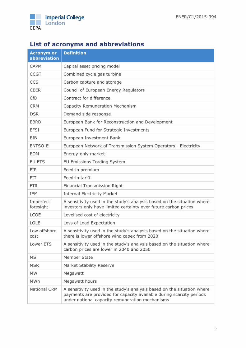
List of acronyms and abbreviations

Acronym or

abbreviation

Definition

CAPM Capital asset pricing model

CCGT Combined cycle gas turbine

CCS Carbon capture and storage

CEER Council of European Energy Regulators

CfD Contract for difference

CRM Capacity Remuneration Mechanism

DSR Demand side response

EBRD European Bank for Reconstruction and Development

EFSI European Fund for Strategic Investments

EIB European Investment Bank

ENTSO-E European Network of Transmission System Operators - Electricity

EOM Energy-only market

EU ETS EU Emissions Trading System

FIP Feed-in premium

FIT Feed-in tariff

FTR Financial Transmission Right

IEM Internal Electricity Market

Imperfect

foresight

A sensitivity used in the study's analysis based on the situation where

investors only have limited certainty over future carbon prices

LCOE Levelised cost of electricity

LOLE Loss of Load Expectation

Low offshore

cost

A sensitivity used in the study's analysis based on the situation where

there is lower offshore wind capex from 2020

Lower ETS A sensitivity used in the study's analysis based on the situation where

carbon prices are lower in 2040 and 2050

MS Member State

MSR Market Stability Reserve

MW Megawatt

MWh Megawatt hours

National CRM A sensitivity used in the study's analysis based on the situation where

payments are provided for capacity available during scarcity periods

under national capacity remuneration mechanisms

ENER/C1/2015-394

10

Acronym or

abbreviation

Definition

No pref rules A sensitivity used in the study's analysis based on the situation where

preferential market rules (e.g., priority dispatch for biomass

generators) are removed after 2020

OCGT Open cycle gas turbine

PCI Project of Common Interest

PHS Pumped hydro storage

PPA Power Purchase Agreement

PRIMES The PRIMES energy model simulates the European energy system and

markets on a country-by-country basis and across Europe for the

entire energy system.

PV Photovoltaics

RES-e Renewable energy sources for electricity

RMP Reference market prices

RO Renewable obligation

ROR Run of river

SOAF Scenario Outlook and Adequacy Forecast

SRMC Short-run marginal cost

TSO Transmission System Operator

TYNDP Ten-Year Network Development Plan

VoLL Value of lost load

WACC Weighted average cost of capital

WACC+ A sensitivity used in the study's analysis based on the situation where

there is a mark-up of 100 and 200 basis points, respectively, on top of

the baseline discount rate for projects

WeSIM The electricity market simulation model used in this study

WeSIM

RES30/EE30

A scenario used in the study's analysis that is based on PRIMES

RES30/30 scenario; and which assumes 30 percent energy efficiency

and 30 percent RES-e penetration by 2030

WeSIM

RES27/EE27

A scenario used in the study's analysis that is based on the PRIMES

EUCO27 scenario, which assumes that the 27 percent energy

efficiency and the 27 percent RES-e targets are met by 2030 This

serves as the baseline scenario.

WeSIM

RES27/EE

Pessimistic

A scenario used in the study's analysis with a combination of lower

levels of demand side response, interconnection, carbon prices and

energy efficiency than the baseline scenario; and the assumption that

the 27 percent RES-e target is still achieved by 2030

ENER/C1/2015-394

11

Acronym or

abbreviation

Definition

WeSIM

RES27/EE30

A scenario used in the study's analysis that is based on the PRIMES

EUCO30 scenario, which assumes that a 30 percent energy efficiency

and a 27 percent RES-e penetration level is achieved by 2030

WeSIM Ref A scenario used in the study's analysis that is based on the EU

Reference Scenario

ENER/C1/2015-394

12

Executive summary

Cambridge Economic Policy Associates (CEPA) was retained by the European Commission

(the Commission) to study EU-, regional- and national-level policy options for supporting

investments into renewable energy sources for electricity (RES-e) in the context of deep

market integration after 2020.

The deployment of new RES-e generating capacity in the EU has traditionally been

supported through measures, such as feed-in tariffs (FITs) and priority dispatch for the

electricity produced from the RES-e installations. These measures have offered high

certainty to investors, and thus lowered the cost of capital required to invest in new

capacity. Overall, this approach provided a combination of an attractive regulatory

framework and appealing RES-e support measures, resulting in a rapid increase in RES-e

capacity across the EU.

Although the support measures have been successful at accelerating RES-e capacity

deployment, their efficiency has been called into question. The scaling-up of RES-e

deployment has brought dramatic cost reductions for some technologies, in particular for

onshore wind and solar photovoltaics (PV). At the same time, some Member States (MS)

have been slow at adjusting their support levels, which has resulted in higher than

necessary costs, and in some cases even abrupt changes to their RES-e support

systems. Furthermore, the increase in the amount of variable RES-e generation has not

been matched with appropriate investments in the transmission grid and measures to

enhance the flexibility of the power system.

The current EU-level framework for supporting new RES-e capacity runs until 2020. It is

characterised by two main elements:

The Renewable Energy Directive 2009/28/EC, which sets binding national targets

for renewable energy, and leaves the MS with discretion in designing and

managing renewable energy support schemes within the boundaries of the EU

State Aid rules.

The Energy and Environment State Aid Guidelines, applicable from 2014 to 2020,

which significantly limit—from a State Aid and internal market perspective—the

design options for national RES-e support schemes. In general and except for

small scale installations, (i) RES-e support levels must be set through competitive

bidding processes; (ii) RES-e producers are increasingly exposed to market prices

and must directly market the electricity they generate; and (iii) RES-e producers

must take on standard balancing responsibilities, unless a liquid intraday market

does not exist.

ENER/C1/2015-394

13

Objectives of the study

Taking into account the above considerations, the objective of this study was to address

the following key questions:

What are the likely paths of EU electricity market developments through 2050,

and how are RES-e shares likely to evolve under those scenarios?

Assuming an energy-only market (EOM) as the only source of revenue, what are

the likely market revenues for each type of RES-e in each MS, assuming no

financial support from public funds?

How sensitive are these estimates to the key variables, including carbon prices,

the amount and design of capacity remuneration mechanisms (CRMs), the

deployment of demand side flexibility, and the degree of interconnectivity?

What is the quantitative range of the investment challenge for RES-e?

What policy options can be employed to mitigate the investment challenge,

focusing on key aspects, such as: (1) the cost of capital, as a function of risk

premiums due to different market and support designs; and (2) the certainty and

magnitude of the different revenue streams for different technologies, as well as

windfall profits?

Approach

The analytical framework applied in this study consists of three core components. First,

RES-e market revenues for a range of future scenarios were estimated using WeSIM, an

hourly simulation model of the European electricity market. These simulation results

served as an input into our financial model where they were used alongside estimates of

generator costs and discount rates to assess the viability and funding gaps of each RES-

e technology under different scenarios and support options. In this context, we defined

the 'viability gap' as the difference (typically a shortfall) between the market revenues

and the levelised cost of a RES-e installation or technology in a MS at a particular point

in time. The 'funding gap' represents a measure of the cost of support required under a

support option, needed to eliminate the viability gap of those RES-e projects that are

required for meeting the decarbonisation targets. These metrics allowed us to identify

which support options might meet the respective investment challenge with the least

amount of support, as well as the relative margins between them. The last component of

the framework consists of a systematic assessment of policy options, using the results

from the quantitative analyses, as well as qualitative reasoning.

Scenarios

Various scenarios were modelled to analyse the financial implications for RES-e of

possible market developments through to 2050. In addition to these possible future

states of the world, several sensitivities were performed around our baseline scenario

(WeSIM RES27/EE27, described below). Key features and assumptions of the modelled

scenarios and sensitivities are summarised in the table below.

Scenario Key features

Main scenarios

1 WeSIM RES27/EE27 Based on the PRIMES EUCO27 scenario, which assumes that the 27 percent energy efficiency and the 27 percent RES-e targets are met by 2030. This serves as the baseline scenario.

2 WeSIM RES27/EE30 Based on the PRIMES EUCO30 scenario, which assumes that a 30 percent energy efficiency and a 27 percent RES-e penetration level is achieved by 2030.

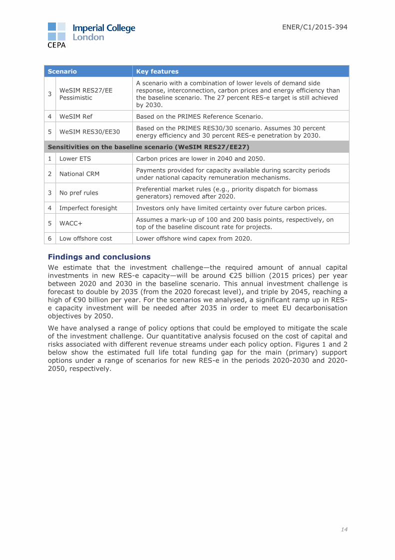
ENER/C1/2015-394

14


3 WeSIM RES27/EE Pessimistic

A scenario with a combination of lower levels of demand side response, interconnection, carbon prices and energy efficiency than the baseline scenario. The 27 percent RES-e target is still achieved by 2030.

4 WeSIM Ref Based on the PRIMES Reference Scenario.

5 WeSIM RES30/EE30 Based on the PRIMES RES30/30 scenario. Assumes 30 percent energy efficiency and 30 percent RES-e penetration by 2030.

Sensitivities on the baseline scenario (WeSIM RES27/EE27)

1 Lower ETS Carbon prices are lower in 2040 and 2050.

2 National CRM Payments provided for capacity available during scarcity periods under national capacity remuneration mechanisms.

3 No pref rules Preferential market rules (e.g., priority dispatch for biomass generators) removed after 2020.

4 Imperfect foresight Investors only have limited certainty over future carbon prices.

5 WACC+ Assumes a mark-up of 100 and 200 basis points, respectively, on top of the baseline discount rate for projects.

6 Low offshore cost Lower offshore wind capex from 2020.

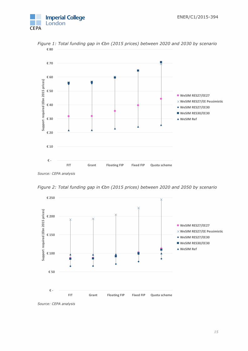
Findings and conclusions

We estimate that the investment challenge—the required amount of annual capital

investments in new RES-e capacity—will be around €25 billion (2015 prices) per year

between 2020 and 2030 in the baseline scenario. This annual investment challenge is

forecast to double by 2035 (from the 2020 forecast level), and triple by 2045, reaching a

high of €90 billion per year. For the scenarios we analysed, a significant ramp up in RES-

e capacity investment will be needed after 2035 in order to meet EU decarbonisation

objectives by 2050.

We have analysed a range of policy options that could be employed to mitigate the scale

of the investment challenge. Our quantitative analysis focused on the cost of capital and

risks associated with different revenue streams under each policy option. Figures 1 and 2

below show the estimated full life total funding gap for the main (primary) support

options under a range of scenarios for new RES-e in the periods 2020-2030 and 2020-

2050, respectively.

ENER/C1/2015-394

15

Figure 1: Total funding gap in €bn (2015 prices) between 2020 and 2030 by scenario

Source: CEPA analysis

Figure 2: Total funding gap in €bn (2015 prices) between 2020 and 2050 by scenario


€ -

€ 10

€ 20

€ 30

€ 40

€ 50

€ 60

€ 70

€ 80

FIT Grant Floating FIP Fixed FIP Quota scheme

Sup

po

rt r

eq

uir

ed

(€

bn

20

15

pri

ces)

WeSIM RES27/EE27

WeSIM RES27/EE Pessimistic

WeSIM RES27/EE30

WeSIM RES30/EE30

WeSIM Ref

€ -

€ 50

€ 100

€ 150

€ 200

€ 250

€ 300


Sup

po

rt r

eq

uir

ed

(€

bn

20

15

pri

ces)

WeSIM RES27/EE27


WeSIM RES27/EE30

WeSIM RES30/EE30

WeSIM Ref

ENER/C1/2015-394

16

While these results suggest that FIT and grant schemes may result in the lowest cost of

support, there is a significant variation in the funding gap between the different

scenarios (e.g., €22 billion to nearly €56 billion in the 2020-2030 period for FIT). Our

qualitative assessment—which considered a broader range of social costs that are

generally more difficult to quantify—concluded that overall social costs would be higher

under a FIT, compared to a Floating feed-in premium (Floating FIP) scheme. Grants, on

the other hand, score lower on implementability criteria. Thus, when all social costs are

considered, Floating FIP schemes are the most likely to meet the RES-e targets at least

(social) cost.

Results from our quantitative analysis also suggest that, in 2020, we may be at the start

of a transition away from having to subsidise several major RES-e technologies. This

transition is being partly driven by technology cost improvements, as well as by a

reduction in investor risk perceptions as several RES-e technologies reach maturity. If

the wholesale electricity markets can deliver the prices that our simulation model

projects, based on the PRIMES scenarios, much of the RES-e capacity needed to meet

the EU decarbonisation goals would receive sufficient remuneration, without public

support, to recover their investment costs.

As noted above, the level of electricity market revenues is crucial for this transition to

materialise. In fact, our analysis shows that increasing electricity market revenues are a

more important factor in improving RES-e viability than technology cost improvements.

Our simulations suggests that electricity market prices would have to more than double

in real terms between 2020 and 2050 for the transition to viability to take place.

Increasing carbon prices, which are based on the assumption that the current EU ETS

system will be credibly reformed, drives much of the projected increase in electricity

prices, especially from 2030 onwards. In particular, if reforms enable ETS and electricity

market prices to rise, and conventional generators start facing a much higher cost of

carbon emissions, many more investors will find that electricity market revenues are

sufficient to remunerate RES-e investments, and we see that materially feeding through

to RES-e viability gaps in our modelling from 2025 and 2030. However, this effect may

be dampened if there are macroeconomics-driven upward shifts in the discount rates, or

if investors do not find, for example, the carbon market reforms sufficiently credible to

be factored into their investment analysis. Thus, policy risk is the key factor that could

endanger the transition to RES-e viability.

The required market reforms will also lead to increases in consumer bills (although they

may be mitigated by lower RES-e support costs), which might be politically challenging,

and could lead to a lower public acceptance of climate and energy policies. This, in turn,

may influence investors’ perception of the credibility of the commitment to the

decarbonisation objectives. Policy options may, to some extent, mitigate investor risk

perception, and therefore the level of support required. However, in the best interest of

electricity customers, the objective of the policy option should be to achieve the lowest-

cost RES-e mix, and to minimise market distortions, whatever the market conditions

turn out to be. Our qualitative assessment focused on identifying such policy options. We

found that increasing the scope of RES-e support auctions across countries and

technologies should lead to the lowest-cost RES-e mix.

Recommendations

In developing our recommendations, we considered that the primary policy objective

should be to meet future (2030) RES-e targets and 2050 decarbonisation

objectives at the least social cost. This should be achieved by providing financial

support to RES-e investments that would not materialise in the absence of such support,

given insufficient electricity market revenues to remunerate for such investments (i.e., a

viability gap exists).

ENER/C1/2015-394

17

Cost effectiveness in this context refers to social costs1, recognising the fact that there

are inherent tensions and trade-offs between costs to investors and costs that accrue to

consumers (e.g., lowering the cost to investors may result in higher cost to consumers if

it is achieved by means that create incentives for the inefficient operation of RES-e

generators).

Since the primary policy objective should be to obtain the least-cost RES-e mix required

to meet the RES-e target, some emerging technologies—at least those that are not

required for meeting the targets—may not receive much support under our proposed

mechanism. Although, we understand that policy makers may wish to pursue other

objectives through energy/ RES policies—such as, resource diversity, domestic job

creation or supporting innovation in emerging RES-e technologies. We note that pursuing

such goals—in addition to meeting the RES-e target—is likely to result in a higher cost of

meeting the primary objective. Our recommended policy option is flexible, and could

allow the incorporation of additional policy objectives—assuming that the additional costs

are acceptable—but without changing the nature of the primary support mechanism. For

example, emerging technologies, those that would likely not succeed in a technology-

neutral auction, could be excluded from the primary support mechanism, and receive

technology-specific support through an auxiliary mechanism. Based on our current

modelling, we expect that many RES-e technologies, including offshore wind, would clear

in the primary support mechanism, while it might take some time for other technologies,

such as tidal range, to fall into this category.

We have factored into our recommendations lessons learned from current and past

support mechanisms implemented in Europe and around the world. These practical

lessons have highlighted the importance of mechanisms that are not just well-designed,

but also politically feasible and implementable.

The market simulations that were performed for this study have also informed our

recommendations. Although they cover a number of future scenarios and a range of

policy options, our recommendations are not dependent on these results nor the

assumptions that underlie them. The recommended support mechanisms are robust to

changing market conditions. This is important, since the future is inherently uncertain,

and thus the support mechanism put in place should be designed to meet the primary

objective under all circumstances.

An important implication of cost efficiency of the chosen support mechanism is that RES-

e generators receiving support are well-integrated into the wholesale market and that

they respond to market signals. Thus, when assessing the policy options, we considered

potential market-distorting behaviour and their associated costs.

Taking into account the above considerations, we have concluded, based on our

qualitative and quantitative assessment, that in terms of economic efficiency, the best

way to achieve the primary objective is to provide RES-e support via a single,

primary support mechanism. This mechanism would:

Be technology-neutral—allowing direct competition among different types of

non-viable RES-e technologies for support to provide the new generation capacity

required to achieve renewables targets.2 This approach is most likely to minimise

the total cost of RES-e support by avoiding deadweight losses created in

technology-specific schemes, given that the asymmetric information problem3

regarding technology costs is likely to persist between investors and regulators.

Technology-neutral mechanisms do not rely on policymakers’ knowledge of

1 Social costs are total costs to society. 2 This could, for example, mean PV and offshore wind competing in the same auction, assuming both are not

viable without support. 3 RES investors have more accurate information about current and future technology costs than policymakers.

ENER/C1/2015-394

18

technology and other costs. Instead, competitive pressure in support auctions will

provide investors with an incentive to reveal these costs in their bids. This

approach would also support innovation, since offering a more cost-effective

technology would put the RES-e investors in that technology at a competitive

advantage in the support auction. RES-e investors would also have an incentive

to efficiently site their generators in locations where the overall (social) cost of

generating clean energy is the lowest. This rests on the assumption that the

charges RES-e generators face, including transmission charges, are cost-

reflective. If they were not, the investors would still factor them into their

investment decision, but the siting of the RES-e generators may not be efficient.

This does not detract from the merits of the proposed support mechanism: the

distortions occur in other parts of market design, not RES-e support, and that is

where they should be remedied. It would not be desirable to attempt to remedy

such imperfections as part of RES-e support mechanism design.

Allocate RES-e support via competitive auctions—these auctions should be

designed in a manner that maximises potential competition. Establishing

competitive allocation mechanisms alone may not be sufficient to achieve efficient

outcomes. The level of potential competition should be continuously monitored,

and safeguards should be put in place to ensure that auction results are truly

competitive. An effective way of increasing competition is to open up RES-e

support auctions to cross-border competition. To achieve this, we make the

following recommendations:

o First-come-first-served and other non-competitive allocation

mechanisms should be phased out—several mechanisms implemented in

the past relied on non-competitive allocation mechanisms (e.g., FIT), which

likely resulted in overall costs that were higher than necessary.

o Auctions in the primary mechanism should not be designed to

distinguish between technologies beyond excluding technologies that

are viable without support (e.g., there should not be technology banding).

All cleared RES-e should receive the uniform auction-clearing prices as RES-e

support.

o If auctions allow for cross-border participation, they should be

designed as locational auctions, whereas RES-e support is dependent on

the auction-clearing price in the market where the RES-e installation is (or will

be) located. This approach recognises that the market price of electricity may

differ between markets, and thus ensures that RES-e generators are not

overcompensated with respect to their viability gap.

o Administrative procedures for determining the level of support should

be used as a last resort—a technology-neutral approach should maximise

the level of competition, especially if it covers a relatively large geographic

area. If, however, potential competition is not sufficient to achieve a

competitive outcome (e.g., concentration of bidders is high) then the reasons

for the lack of competition and potential solutions (e.g., merging a small

national scheme into a larger regional scheme) should be explored,4 before

support levels are set administratively. Support levels should be set in an

administrative manner only as a fall-back option.

o We recommend assessing the level of competition before RES-e

support auctions are cleared. This would involve analysing bids before

each round of competitive allocation to check whether any bidder has the

ability and/or the incentive to distort the auction-clearing price.

4 We understand that these solutions may be politically challenging, but the potential benefits could be significant.

ENER/C1/2015-394

19

The different types of policy options considered in this study do not perform equally.

Auxiliary options (preferential market rules, carbon contracting, and development

finance) would not provide sufficient support for all new RES-e required to achieve

renewable targets, and thus are not suitable as a means of primary RES-e support.

Of the investment aid options, grants in particular could in theory achieve the RES-e

targets cost-efficiently; however large upfront costs, as well as potential defaults by

investors, could make it challenging to implement and maintain such mechanisms on a

large scale. Although this could be mitigated by issuing grant payments tied to the

achievement of specific project milestones, relying on grants as a primary mechanism

for RES-e support is largely uncharted territory in the world of RES-e support. To our

knowledge, grants have only been used for RES-e support on a relatively small scale, at

least compared to the RES-e investment challenges in Europe. Grants would also raise

unique implementation challenges, such as whether support should be provided for MWh

of energy generated or MW of installed capacity. Given the scale of the RES-e

investment challenge in Europe, using grants on a large scale might also be susceptible

to fraud and public acceptance challenges. Grants could be used to meet auxiliary

objectives, such as supporting innovation to develop immature technologies, if it is

desired.

Of the operating aid options, FIT and Fixed FIP are inferior to other options such

as Floating FIP and RO, and should therefore be phased out. FIT heavily relies on

administratively set parameters. Past implementation of FIT has resulted in

overcompensation and abrupt policy changes. Furthermore, FIT offers limited

opportunity for integrating RES-e into the wholesale markets, as generators with a FIT

are shielded from market prices. While the current Renewable Energy Directive allows for

small-scale RES-e to receive FITs, small-scale RES-e installed in large volumes can have

significant negative impacts on the wholesale market, as evidenced by the experience of

some MS. Therefore, we do not recommend allowing FIT to all small-scale RES-e

based on size alone. FIT for small-scale RES-e should only be allowed if total

capacity of small-scale RES-e does not exceed a total capacity threshold, such

that small-scale RES-e in the aggregate does not have a material impact on the

wholesale market. Above this threshold, small-scale RES-e could be supported

via an auxiliary mechanism as described below.

There has been little practical experience with pure Fixed FIP schemes. We consider

them inferior to floating premium schemes. Although the level of support would be set in

competitive auctions, RES-e investors receiving fixed premia would face higher risks and

costs than under a Floating FIP, given the absence of wholesale price risk protection in

the scheme. Also, there is limited practical experience with large-scale Fixed FIP

schemes. For this reason, we do not recommend the implementation of these types of

support mechanisms.

From a theoretical point of view, Renewable obligation (RO, or Quota) schemes could

achieve a similar cost-effective outcome as Floating FIP schemes. In practice, however,

not all RO mechanisms have performed well. While the joint Swedish-Norwegian RO

scheme is generally viewed as reasonably well-functioning, other MS (e.g., UK) have

replaced them with other mechanisms. That should, however, not be a reason to

abandon existing mechanisms in other MS if they perform reasonably well. Therefore,

we recommend assessing whether the current RO schemes are on track to meet

the RES-e targets and whether those targets are being met efficiently.

The primary appeal of Floating FIP schemes is that they best address the main risks

associated with RES-e support: regulatory and policy risk. Unlike other options, Floating

FIP can be tied to a Contract for Differences (CfD), under which RES-e investors have

ENER/C1/2015-394

20

legal recourse in case the government reneges on its commitments.5 Also, because the

strike price of the CfD is fixed and guaranteed, it removes wholesale market and policy

risk related to market design (e.g., ETS).

Therefore, after 2020 we recommend transitioning to a Floating FIP as the

default primary mechanism for RES-e support in those MS that do not currently

have an RO mechanism in place.

MS that currently support RES-e using a mechanism other than Floating FIP or

RO, should converge to Floating FIP (although, some MS could join a neighbour’s

RO to create a joint scheme).

MS that already have a Floating FIP should gradually modify their mechanisms so

that the schemes offered to new capacity converges to the proposed design

described below.

Overall, Floating FIP performed better than RO in our assessment, but the

incremental benefits associated with Floating FIP may not justify transitioning to

it from an existing RO scheme. However, for MS that have neither Floating FIP

nor RO, we recommend to implement a Floating FIP, since that already appears

to be the direction of travel in much of Europe.

Recommended primary option for RES-e support

We note that the choice of scheme design is as important as its implementation—

therefore individual design features should be implemented, at a minimum, to

incorporate the design features (harmonisation, eligibility rules, strike price, reference

market price), described below. We recommend to implement Floating FIP with the

following design features.

Harmonisation

Although not necessarily required for maximum economic efficiency, it would be

preferred that the same or similar option designs are implemented across the MS.

Harmonisation would help investors, and it may also facilitate regional cooperation in the

future. Harmonisation would involve the alignment of:

Eligibility rules—defining what types of RES-e generators and under what terms

are allowed to participate in the RES-e support scheme. With harmonisation, the

same general principles would apply across MS.

Timing of auctions—auctions in each MS should be timed in such a manner that

potential RES-e investors can relatively easily compare the investment

opportunities.

Other key design elements of the auctions—for a future regional cooperation, it

would be desirable to align the key design elements, so that RES-e investors can

easily assess the value of the opportunity of participating in multiple schemes.

Eligibility rules

Eligibility rules establish which RES-e generators are allowed to participate in the support

scheme. It is not just a function of technology type, but also, for example, time and

location. It is not desirable to support RES-e technologies that are viable on their own

(i.e., from market revenues alone). Our modelling shows that in many countries under

the considered scenarios the main RES-e technologies may become viable by 2030.

Thus, these technologies should not be eligible by 2030 to participate in a RES-e support

scheme.

5 This feature may be part of other types of support schemes, depending on the legal system.

ENER/C1/2015-394

21

We recommend assessing technology viability ex-post, using a backward-looking

analysis of a three- to five-year period preceding each RES-e support auction. If a RES-e

technology was viable in each of those years, it should not be eligible for future support.

The viability assessment should be conducted in an independent manner, without any

bias from RES-e investors. The economics of RES-e technologies close to viability is well-

understood; therefore, independent studies—such as those conducted to estimate the

cost of a hypothetical best new entrant in capacity markets—could be relied upon.

We recommend that participation in the primary support mechanism should preclude a

generator from preferential market rules. In line with current State Aid Guidelines, RES-e

that are eligible for the primary support mechanism and receive support through it,

would not qualify for exemption from balancing responsibility. Similarly, to avoid the

potential distortion of wholesale markets identified in our qualitative analysis, we

recommend that they do not qualify for priority dispatch.

Strike price

Strike price is the uniform price received by all RES-e capacity cleared in a RES-e

support auction. The strike price should be set by the bid of the marginal RES-e capacity

cleared in the auction.6

Reference Market Price (RMP)

The choice of the RMP should reflect the available market revenue for producers in a MS.

We recommend that an averaging period of at least a day be used to set the RMP, as

doing so should give generators the incentive to respond to market signals within that

period. Longer reference periods (e.g., monthly or annual) may be beneficial for market

integration, but the marginal benefit from doing so should be weighed up against any

genuine impact of the basis risk that would create on investors’ cost of capital–this might

need to be considered on a case-by-case basis.

We believe that the proposed approach strikes the best balance between achieving

higher levels of market integration and transferring a bearable share of the risks for the

RES-e producers.

Adaptations for political constraints

We recognise that although the proposed primary support option is highly attractive from

an economic point of view, some MS may find it politically challenging to implement in

practice, even if argued for robustly. If political or other constraints make its

implementation infeasible, we propose to implement a version of it with as many of the

proposed features as possible. For example, if technology-neutrality is politically

unacceptable, a version of the Floating FIP scheme could be implemented with

technology-specific features (such as multiple pots or administered technology-specific

caps as applied in the UK CfD), with all other design features as described above.

Although this would not be a scheme that maximises social welfare, it would yield the

best outcome, given the political constraint.

Auxiliary support options

Provision of technology-specific support

If additional RES-e objectives are desired, in addition to meeting the RES-e targets, such

as supporting innovation in emerging RES-e technologies, then auxiliary technology-

specific support mechanisms could be implemented. RES-e technologies eligible for this

6 For clarity, we do not recommend the inclusion of administered technology-specific strike price caps as implemented in the UK CfD auctions to date.

ENER/C1/2015-394

22

type of support should not be viable without support, nor would they be able to obtain

support from the primary mechanism (because their costs are too high to be selected for

support in a competitive mechanism).

These auxiliary mechanisms would be separate from the primary mechanism, and they

should not interfere with the primary mechanism in any way. We consider that the

primary rationale for this mechanism would be to improve dynamic efficiency (i.e.,

reduce the cost of meeting future RES-e targets by supporting innovation today,

resulting in a reduced social cost over the long term). Since potential benefits from

dynamic efficiency are not apparent, and may vary case by case, we would recommend

that a cost-benefit analysis be conducted before a technology-specific, innovation-

focused support mechanism is introduced (or maintained) with the rationale of improving

dynamic efficiency.

There are several options available to provide innovation-focused support, including FIT,

FIP, grants and development finance. We recommend the allocation of FIT, FIP or grant

support, to the extent possible, via competitive mechanisms. By its nature, development

finance is likely to need to be allocated through an administrative process. Given the

relative advantages of Floating FIP over other options, we consider it might be the best

form of support for an auxiliary, technology-specific support scheme.

Development finance

While there is a continuing need for interventions from public finance institutions, based

upon concrete financing issues faced by projects, we understand that in many cases

support is already provided such that further intervention in this area may not be

required today. For instance, the European Investment Bank (EIB) and the Commission

recently established the €21 billion European Fund for Strategic Investments (EFSI)

targeted at lending to riskier technologies, sectors and countries, as well as supporting

the EIB in the provision of subordinated debt and guarantees to boost project credit

ratings.

However, we consider that should concrete cases be identified where there is an unmet

financing gap, we recommend a blended finance approach in which either commercial

financiers or public development finance providers would use budgetary resources to

soften the terms of finance provided.7 The justification for this softening of terms would

be to prevent financial market failures, such as balance sheet limits or the effect of

novelty on investors’ risk aversion, from undermining the viability of projects. It would

be used alongside primary support mechanisms. The focus of this intervention would

therefore be on bridging the financing gap for projects that are close to being

investable/bankable but where specific problems mean that they fail to attract sufficient

finance, even with the support of one of the primary options being available. This would

be targeted at less mature technologies, with either higher costs and/or technology risk–

a current example of such a technology with eligible projects might be offshore wind–or

where there is a lack of investor/lender confidence in government commitment to

support schemes in a particular MS.

Preferential market rules

We focused on two preferential market rules: priority dispatch and exemption from

balancing responsibility.

7 We envisage that this could be achieved in practice through blended finance. For funded products such as subordinated loans, this might involve use of a grant to provide an interest rate subsidy, which would reduce

the risk reflectiveness of pricing relative to prices that the market would charge. For credit or event-specific guarantees the grant might be used to set the guarantee fee at a level that is not fully risk-reflective.

ENER/C1/2015-394

23

We recommend phasing out priority dispatch for all RES-e generators. Our

findings suggest that priority dispatch on its own is detrimental to RES-e market

revenues, and results in significant social (deadweight) cost. Priority dispatch as a

standalone means of RES-e support would be detrimental to RES-e viability because it

inefficiently supresses the electricity price for all RES-e, and thus increases their viability

gap. Furthermore, priority dispatch is not valuable (on its own) to individual RES-e

generators when they do not receive any other form of support except priority dispatch.

This is because most RES-e generators (e.g., wind, solar) have zero- or near-zero

marginal costs and under our proposed mechanism would receive no support when

market prices are negative; thus, priority dispatch would have no impact on them. Under

our proposed mechanism, non-zero marginal cost technologies (e.g., biomass) would

have a reduced incentive to be dispatched during hours when their marginal cost is

above the market price, since they would often suffer losses, unless a separate funding

mechanism were in place to recuperate those losses. Without priority dispatch they

would generate less frequently, but their profits would be higher because they would not

generate in periods when the electricity price is lower than their marginal cost.

In the past, priority dispatch was offered in conjunction with FITs for many RES-e

generators. Since priority dispatch guaranteed maximum generation, and the unit price

paid was not function of the market price, RES-e generators benefited from it.

Exemption from balancing responsibility could be granted in exceptional cases.

Imbalance costs do not feature among the main concerns of RES-e investors in most

MS; however, we recognise the fact that some balancing markets in the EU are less

developed then others. If imbalance prices are not cost-reflective, RES-e generators (as

well as other market participants) may be exposed to inefficiently high balancing costs.

Therefore, on a temporary and case-by-case basis these generators could receive an

exemption from balancing responsibility until the balancing market design and pricing is

improved. This would not be a form of RES-e support to address the RES-e viability gap,

but rather an offset to unreasonably high costs caused by imperfect balancing market

design.

Further recommendations

Regional cooperation

In theory, support mechanisms implemented on a regional- or EU-wide basis could

deliver significant efficiency improvements over national mechanisms. However, an EU-

wide implementation of the proposed primary RES-e support mechanism appears at

present challenging, primarily due to a lack of political feasibility. Our modelling of

partial opening of national schemes has highlighted the potential benefits in terms cost

reductions, but also showed that these benefits will diminish as RES-e viability improves.

Once the majority of RES-e becomes viable, inefficiencies associated with national-only

RES-e schemes also become smaller. These inefficiencies relate only to non-viable RES-

e, since for viable RES-e, investors should have the incentive (based on market signals)

to site their generators at the best locations, and thus avoid any inefficiencies associated

with inefficient siting.

With respect to regional coordination, we recommend:

The long-term objective of regional cooperation should be to have joint schemes

that cover relatively large geographic areas in order to benefit from the best RES-

e potential. We note, however, that in our analysis viability of many technologies

is achieved by 2030, while in other scenarios it takes longer. A faster path to

viability limits the benefits from regional cooperation.

ENER/C1/2015-394

24

Gradual opening of existing Floating FIP and RO mechanisms to neighbouring

markets should therefore be considered, with the longer-term objective of

creating jointly-administered schemes.

Since there may be significant differences in national regulations that affect RES-

e (e.g., taxation, transmission charging regimes), it should be monitored whether

these result in any distortions in RES-e support.

Jointly-administered mechanisms will require a cooperation agreement between

participating MS, including a potential sharing mechanism for efficiency gains

from regional cooperation, which would involve financial transfers between MS

where the efficiency gains are unevenly distributed. The participating MS may

also have to set up a joint entity to implement and manage the joint mechanism.

Transition to the recommended mechanism

We do not recommend replacing all existing support mechanisms immediately. While

some imperfections may currently exist with national mechanisms, any change in policy

and move to a new RES-e mechanism will inherently involve some policy risk. Since

policy risk is one of the main concerns for investors, a higher level of policy risk may

increase the cost of capital, and thus overall system costs, while at the same time

transition to a new RES-e support scheme may deliver only marginal benefits. Therefore,

prior to each transition, it should be assessed whether the benefit of replacing an

existing scheme with a more efficient form of support (as recommended in this report)

outweighs the increased costs, including the impact of higher policy risk on the cost of

capital. We consider that this may not be the case for some of the existing Floating FIP

and RO schemes.

It is critical that the transition to new schemes is performed in a transparent manner and

is communicated to investors in advance. We recommend a two- to three-year transition

from existing schemes to new ones. It is also critical to provide assurance that

retroactive changes will not be made.

Market design and overall energy policy

We consider that our recommended mechanisms are robust to changing market

conditions. For example, if the EU ETS is not reformed in a credible manner that would

result in higher energy market revenues, RES-e investors would, all else equal, increase

their bids in the RES-e support auctions, and thus would likely receive more revenue

through support payments (assuming funding is available). Nevertheless, overall market

design is critical, because imperfections would either result in higher support costs or

lower investments in RES-e.

Therefore, we recommend a periodic review of the performance of EU markets in the

context of RES-e support. This could include, for example, reviewing distortions to cross-

border trade (e.g., due to non-cost reflective transmission charges in one MS) that could

inefficiently distort RES-e investments across multiple countries.

ENER/C1/2015-394

25

Résumé

Cambridge Economic Policy Associates (CEPA) a été retenu par la Commission

Européenne (la Commission) pour étudier les différentes options de politiques au niveau

européen, régional et national pour soutenir les investissements dans les énergies

renouvelables (EnR) dans le contexte d’approfondissement de l’intégration du marché

après 2020.

Le déploiement de nouvelles capacités de génération d’EnR dans l'UE a

traditionnellement été soutenu par des mesures telles que le tarif de rachat (FIT) et le

principe de priorité de distribution en faveur de l’électricité produite par les installations

d’EnR. Ces mesures ont offert un niveau élevé de certitude aux investisseurs, et ont

réduit de cette façon le coût du capital requis pour investir dans une capacité

supplémentaire.

Bien que les mesures de soutien aient réussi à accélérer le déploiement de capacité

renouvelable, leur efficacité a été remise en question. L'intensification du déploiement

des EnR a considérablement réduit les coûts de certaines technologies, en particulier

pour l'éolien terrestre et l'énergie solaire photovoltaïque (PV). Simultanément, certains

Etats membres (EM) ont lentement ajusté leur niveau de soutien, entraînant des coûts

plus élevés que nécessaires, et dans certains cas mêmes, entraînant des changements

abrupts dans les systèmes de soutien aux EnR. De plus, l'augmentation du niveau de

production à partir de sources renouvelables variables n'a pas été suivie par les

investissements adéquats dans le réseau de transmission ou dans l'augmentation de

flexibilité du système électrique.

L'actuel cadre européen pour le soutien à la capacité renouvelable supplémentaire dure

jusqu'à 2020. Il est caractérisé par deux principaux éléments:

Premièrement, la directive relative aux énergies renouvelables 2009/28/EC qui établit

des objectifs nationaux contraignants en matière d'énergie renouvelable, et laisse aux

Etats membres un pouvoir discrétionnaire dans la conception et la gestion des systèmes

de soutien aux énergies renouvelables dans les limites fixées par les règles de l'UE

relatives aux aides d'Etat.

Deuxièmement, les lignes directrices concernant les aides d'Etat à la protection de

l'environnement et à l'énergie, valables de 2014 à 2020, qui limitent significativement

les options pour la conception de systèmes nationaux de soutien aux EnR, d'un point de

vue des aides d'Etat et du marché intérieur. En général, à l'exception des installations de

petite taille: (i) les niveaux de soutien aux EnR doivent être fixés par des mécanismes

concurrentiels contraignants; (ii) les producteurs d'EnR sont exposés de manière

croissante aux prix de marché et doivent directement mettre sur le marché l'électricité

qu'ils produisent; et (iii) les producteurs d'EnR doivent assumer les responsabilités

standards en matière d'équilibrage, à moins qu'il n'existe pas de marché intra journalier

liquide.

Objectifs de l’étude

Prenant en compte les considérations ci-dessus, l’objectif de cette étude était de

répondre aux questions clés suivantes :

Quelles sont les voies probables de développement du marché européen de

l’électricité d’ici 2050, et comment la part d’électricité à partir de sources

renouvelables risque-t-elle d’évoluer selon différents scenarios ?

En supposant que la seule source de revenus soit le marché de l’électricité,

« energy-only market » (EOM), quels sont les revenus de marché probables pour

ENER/C1/2015-394

26

chaque type d’EnR dans chaque EM, en supposant qu’il n’y ait aucun soutien

provenant de fonds publics ?

A quel point ces estimations sont-elles sensibles aux variables clés, incluant le

prix du carbone, le montant et la conception des mécanismes de rémunération de

la capacité, le déploiement de la flexibilité de la demande, et le degré

d’interconnexion ?

Quelle est la fourchette de l’enjeu en termes d’investissements dans les EnR ?

Quelles sont les options de politiques qui peuvent être utilisées pour atténuer

l’enjeu de l’investissement, en se concentrant sur les aspects clés, tels que : (1)

le coût du capital, fonction de la prime de risque due aux différents marchés et

mécanismes de soutien ; et (2) la certitude et l’ampleur des différents flux de

revenus pour différentes technologies, ainsi que les bénéfices inattendus ?

Approche

Le cadre analytique utilisé dans cette étude comprend trois éléments principaux.

Premièrement, les revenus de marché pour les EnR pour une gamme de scénarios futurs

ont été estimés utilisant WeSIM, un modèle de simulation horaire du marché de

l’électricité européen. Ces résultats de simulation servent comme intrants dans notre

modèle financier où ils ont été utilisés avec des estimations de coûts de production et de

taux d’actualisation afin d’évaluer les écarts de viabilité financière et de financement

pour chaque technologie EnR selon différents scénarios et différentes options de soutien.

Dans ce contexte, nous avons défini « l’écart de viabilité » comme la différence

(généralement un déficit) entre les revenus de marché et le coût normalisé d’une

installation EnR ou d’une technologie EnR dans un EM à un point particulier dans le

temps. L’ « écart de financement » représente une mesure du coût de soutien requis

selon une option de soutien, nécessaire pour éliminer l’écart de viabilité des projets EnR

requis pour atteindre les objectifs de décarbonisation. Ces mesures nous ont permis

d’identifier quelles options de soutien pourraient aider à relever l’enjeu d’investissement

respectif avec le moindre niveau de soutien, ainsi que leurs écarts relatifs. Le dernier

élément du cadre analytique comprend une évaluation systématique des options de

politiques, utilisant les résultats de nos analyses quantitatives, ainsi qu’un raisonnement

qualitatif.

Scénarios

Différents scénarios ont été modélisés afin d’analyser les implications financières pour

chaque EnR des développements de marché possibles d’ici 2050. En plus des différents

scénarios futurs possibles, plusieurs sensibilités ont été testées autour de notre scénario

de base (WeSIM RES27/EE27, décrit ci-dessous). Les caractéristiques et les hypothèses

clés de ces scénarios et sensibilités modélisés ont été résumées dans le tableau ci-

dessous.

Scénario Caractéristiques clés

Principaux scénarios

1 WeSIM RES27/EE27

Basé sur le scénario PRIMES EUCO27, qui suppose que les objectifs de 27% d’efficacité énergétique et les 27% de production d’électricité à partir de sources renouvelables seront atteints d’ici 2030. Cela a servi de scénario de base.

2 WeSIM RES27/EE30

Basé sur le scenario PRIMES EUCO30, qui suppose qu’un niveau de

30% d’efficacité énergétique et 27% de pénétration de la production d’électricité à partir de sources renouvelables sera atteint d’ici 2030.

3 WeSIM RES27/EE Un scénario qui allie des niveaux inférieurs de réponse de la

ENER/C1/2015-394

27

Scénario Caractéristiques clés

Pessimiste demande, d’interconnexion, de prix du carbone et d’efficacité énergétique par rapport au scénario de base. L’objectif de 27% d’EnR est toujours atteint d’ici 2030.

4 WeSIM Ref Basé sur le scénario de référence PRIMES.

5 WeSIM RES30/EE30 Basé sur le scénario PRIMES RES30/30. Suppose 30% d’efficacité

énergétique et 30% de pénétration des EnR d’ici 2030.

Sensibilités autour du scénario de base (WeSIM RES27/EE27)

1 Bas ETS Prix du carbone inférieur en 2040 et 2050.

2 CRM nationaux Des rémunérations de capacité sont fournies en échange de la capacité disponible lors de périodes de pénurie selon les mécanismes nationaux de rémunération de capacité.

3 Pas de règles préf. Les règles de marché préférentielles (par exemple la priorité de distribution pour les producteurs de biomasse) ont été retirées après

2020.

4 Prévision imparfaite Suppose que les investisseurs ont une certitude limitée concernant les futurs prix du carbone.

5 WACC+ Suppose une majoration de respectivement 100 et 200 points de base au-dessus du taux d’actualisation de base des projets.

6 Bas coût d’offshore Des coûts en capitaux de l’éolien offshore inférieurs à partir 2020.

Résultats et conclusions

Nous estimons que l’enjeu de l’investissement-le montant requis d’investissements en

capital annuels pour la capacité supplémentaire d’EnR- sera autour de €25 milliards (prix

de 2015) par an entre 2020 et 2030 dans le scénario de base8. Cet enjeu

d’investissement annuel est prévu de doubler d’ici 2035 (à partir du niveau prévu pour

2020), et tripler d’ici 2045, atteignant un pic à €90 milliards par an. Selon les différents

scénarios analysés, une augmentation significative dans l’investissement de la capacité

d’EnR sera nécessaire après 2035 afin d’atteindre les objectifs européens de

décarbonisation d’ici 2050.

Nous avons analysé une gamme d’options de politiques qui pourraient être utilisées afin

d’atténuer l’échelle de l’enjeu de l’investissement. Notre analyse quantitative s’est

concentrée sur le coût du capital et les risques associés aux différents flux de revenus

selon chaque option de politique. Les figures 1 et 2 ci-dessous montrent l’écart estimé de

financement des nouvelles EnR le long de la durée de vie complète des projets pour les

principales options de soutien (primaires) selon une gamme de scénarios,

respectivement durant les périodes 2020-2030 et 2020-2050.

8 Veuillez noter que la modélisation financière effectuée dans le cadre de cette étude a été faite sur une base

annuelle. Ainsi, par souci de clarté, veuillez noter que dans cette étude, la période 2020-2030 dure une décennie et la période 2020-2050 trois décennies.

ENER/C1/2015-394

28

Figure 1: Ecart de financement en €mds (prix de 2015) entre 2020 et 2030 par scénario

Source : Analyse de CEPA

Figure 2 : Ecart de financement en €mds (prix de 2015) entre 2020 et 2050 par scénario

Source: Analyse de CEPA

€ -

€ 10

€ 20

€ 30

€ 40

€ 50

€ 60

€ 70

€ 80


Sup

po

rt r

eq

uir

ed

(€

bn

20

15

pri

ces)

WeSIM RES27/EE27


WeSIM RES27/EE30

WeSIM RES30/EE30

WeSIM Ref

€ -

€ 50

€ 100

€ 150

€ 200

€ 250

€ 300


Sup

po

rt r

eq

uir

ed

(€

bn

20

15

pri

ces)

WeSIM RES27/EE27


WeSIM RES27/EE30

WeSIM RES30/EE30

WeSIM Ref

ENER/C1/2015-394

29

Bien que ces résultats suggèrent que le FIT et les subventions directes reviennent le

moins cher en termes de coûts de soutien, il y a une variation significative dans l'écart

de financement entre les différents scénarios (par exemple, €22 milliards à presque €56

milliards durant la période 2020-2030 pour le FIT). Notre évaluation qualitative, qui a

pris en compte une grande variété de coûts sociaux difficiles à quantifier, a permis de

conclure qu'au global les coûts sociaux seraient supérieurs avec un FIT, comparés à un

mécanisme de complément de rémunération variable "Floating Feed-in-Premium" (FIP).

De l'autre côté, les subventions directes ont un score inférieur pour les critères de mise

en place. Ainsi, lorsque l'on prend en compte tous les coûts sociaux, le FIP variable est le

mécanisme le plus susceptible d'aider à atteindre les objectifs d'EnR avec le moindre

coût (social).

Les résultats de notre analyse quantitative suggèrent également qu'en 2020 nous serons

peut-être au début d'une transition qui permettrait d'éviter de subventionner plusieurs

technologies principales d'EnR. Cette transition est en partie due à l'abaissement des

coûts technologiques, ainsi qu'une réduction de la perception du risque par les

investisseurs à mesure que plusieurs technologies EnR deviennent matures. Si les

marchés d'électricité peuvent donner des prix que notre modèle de simulation projette,

basé sur les scénarios PRIMES, alors la plupart de la capacité d'EnR nécessaire pour

atteindre les objectifs européens de décarbonisation recevrait une rémunération

suffisante pour recouvrir leurs coûts d'investissement sans avoir recours à un soutien.

Comme noté ci-dessus, le niveau des revenus de marché de l'électricité est crucial pour

que cette transition se matérialise. En fait, notre analyse montre que l'augmentation des

revenus de marché de l'électricité est un facteur plus important dans l'amélioration de la

viabilité des EnR que l'abaissement des coûts de technologie. Nos simulations suggèrent

que les prix du marché de l'électricité devraient plus que doubler en termes réels entre

2020 et 2050 pour que la transition vers la viabilité se fasse. L'augmentation du prix du

carbone, basée sur l'hypothèse que le système européen actuel de l'ETS sera réformé de

manière crédible, entraîne principalement l'augmentation projetée des prix de

l'électricité, en particulier à partir de 2030. En particulier, si les réformes permettent à

l'ETS et aux prix du marché de l'électricité d'augmenter, et que donc les producteurs

conventionnels subissent un coût plus élevé d'émissions carbone, alors beaucoup plus

d'investisseurs trouveront que les revenus du marché de l'électricité sont suffisants pour

rémunérer les investissements dans les EnR, et nous voyons ceci se matérialiser dans les

écarts de viabilité des EnR que nous avons modélisés entre 2025 et 2030. Cependant,

cet effet peut être diminué si des changements macroéconomiques entraînent une

hausse des taux d'actualisation ou si les investisseurs ne trouvent pas par exemple les

réformes du marché du carbone suffisamment crédibles pour qu'elles soient prises en

compte dans leur analyse d'investissement. Ainsi, le risque politique est le principal

critère qui pourrait mettre en péril la transition vers la viabilité des EnR.

Les réformes de marché requises entraîneront également une hausse des factures

d'électricité (bien que ceci puisse être atténué par des coûts de soutien aux EnR plus

bas), ce qui pourrait être politiquement délicat, et qui pourrait entraîner une moindre

acceptation des politiques du climat et de l'énergie par l'opinion publique. Ceci, en

retour, peut influencer la perception des investisseurs sur la crédibilité de l'engagement

aux objectifs de décarbonisation. Les options de politiques peuvent jusqu'à un certain

point atténuer la perception du risque par les investisseurs, et donc baisser le coût du

soutien requis. Cependant, dans l'intérêt des consommateurs, l'objectif de la politique

choisie devrait être d'atteindre un mix d'EnR au moindre coût et de minimiser les

distorsions de marché, quel que soient les conditions de marché. Notre évaluation

qualitative s'est concentrée sur l'identification de ces politiques. Nous avons trouvé que

le montant de soutien aux EnR via des enchères à travers les pays et les technologies

devrait amener à un mix d'EnR au moindre coût.

ENER/C1/2015-394

30

Recommandations

En développant nos recommandations, nous avons pris en compte que l'objectif

principal de la politique choisie devrait être d'atteindre les objectifs d'EnR

futurs (2030) et les objectifs de décarbonisation d’ici 2050au moindre coût

social. Ceci devrait être atteint en fournissant un soutien financier aux investissements

dans les EnR qui ne se seraient sinon jamais matérialisés en l'absence d'un tel soutien,

dû au fait que les revenus de marché de l'électricité seraient insuffisants pour rémunérer

ces investissements (c.à.d. qu'un écart de viabilité existe).

L'efficacité des coûts dans ce contexte fait référence aux coûts sociaux9, en admettant le

fait qu'il existe des tensions inhérentes et des compromis entre les coûts pour les

investisseurs et les coûts subis par les consommateurs (par exemple, baisser le coût

pour les investisseurs peut entraîner un coût plus élevé pour les consommateurs s'il est

atteint en créant des incitations à la production inefficace de générateurs EnR).

Etant donné que l'objectif principal de la politique choisie devrait être d'obtenir un mix

d'EnR au moindre coût afin d'atteindre les objectifs d'EnR, certaines technologies EnR, au

moins celles qui ne sont pas requises pour atteindre les objectifs, ne recevront peut-être

pas beaucoup de soutien dans notre proposition de mécanisme. Même si nous

comprenons que certains décideurs politiques puissent désirer poursuivre d'autres

objectifs à travers des politiques énergétiques en faveur du renouvelable, telles que la

diversité des ressources, la création d'emplois locaux, ou bien le soutien à l'innovation

pour les technologies EnR émergentes. Nous notons que la poursuite de ces objectifs, en

plus de l'atteinte des objectifs d'EnR, est susceptible d'entraîner un coût plus élevé dans

l'atteinte de l'objectif principal. Notre recommandation de politique est flexible et

pourrait inclure des objectifs supplémentaires de politiques, en supposant que les coûts

supplémentaires soient acceptables, mais ne changerait pas la nature du mécanisme de

soutien principal. Par exemple, les technologies émergentes, celles qui ne seraient

probablement pas gagnantes dans une enchère à technologie neutre, pourraient être

exclues du mécanisme de soutien principal, et recevraient un soutien technologique

spécifique au travers d'un mécanisme auxiliaire. Basé sur notre modèle actuel, nous

estimons que les technologies comme l'éolien offshore pourraient obtenir un soutien

dans le mécanisme principal, tandis que certaines technologies telles que la technologie

marémotrice prendraient du temps avant de tomber dans cette catégorie.

Nous avons pris en compte dans nos recommandations les leçons apprises des

mécanismes de soutien actuels et passés mis en place en Europe et dans le monde. Ces

leçons pratiques ont mis en lumière l'importance de ces mécanismes qui ne sont pas

uniquement correctement conçus mais également politiquement faisables et applicables.

Les simulations de marché qui ont été effectuées pour cette étude nous ont également

aidés à formuler nos recommandations. Bien qu'elles couvrent un nombre de scénarios

futurs et une diversité de choix politiques, nos recommandations ne sont pas

dépendantes de ces résultats ou des hypothèses sous-jacentes. Les mécanismes de

soutien recommandés sont robustes aux changements de conditions de marché. Ceci est

important, étant donné que le futur est de manière inhérente incertain, et que de ce fait

le mécanisme de soutien mis en place devrait être conçu pour atteindre l'objectif

principal dans toutes les circonstances.

Une conséquence importante de l'efficacité des coûts pour le mécanisme de soutien

choisi est que les producteurs d'EnR recevant un soutien seront effectivement intégrés

au marché de l'électricité et répondront donc aux signaux de marché. Ainsi, quand nous

9 Les coûts sociaux sont les coûts totaux pour la société.

ENER/C1/2015-394

31

avons évalué les choix politiques, nous avons pris en compte les comportements de

distorsion de marché et leurs coûts associés.

En prenant en compte les considérations ci-dessus, nous avons conclu, basé sur notre

évaluation quantitative et qualitative, qu'en termes d'efficacité économique, la

meilleure façon d'atteindre l'objectif principal est de fournir un soutien aux EnR

à travers un mécanisme de soutien principal unique. Le mécanisme serait:

Neutre d'un point de vue des technologies- autorisant une concurrence

directe entre différents types de technologies EnR non-viables, afin d'obtenir un

soutien pour fournir la production incrémentale requise pour atteindre les

objectifs d'énergie à partir de sources renouvelables10. Cette approche est

susceptible de minimiser le coût total du soutien aux EnR en évitant les pertes

sèches créées par les mécanismes de soutien à des technologies spécifiques étant

donné que le problème d'information asymétrique11 concernant les coûts de

technologies est susceptible de perdurer entre les investisseurs et les régulateurs.

Les mécanismes neutres d'un point de vue technologique ne reposent pas sur la

connaissance des décideurs politiques en matière de technologies et d'autres

coûts. A l'inverse, la pression concurrentielle dans les enchères de mécanismes

de soutien fournira aux investisseurs une incitation à révéler leurs coûts dans

leurs offres. Cette approche soutiendrait également l'innovation, étant donné

qu'offrir une technologie plus efficace en termes de coûts placerait les

investisseurs dans les EnR à un avantage compétitif dans les enchères de soutien.

Les investisseurs dans les EnR auraient également une incitation à localiser de

manière efficace leur site de production où le coût global de production d'énergie

propre est le moins cher. Ceci repose sur l'hypothèse que les charges que les

producteurs d'EnR subissent, incluant les coûts de transmission, soient

représentatives des coûts. Si elles ne le sont pas, les investisseurs les incluraient

quand même dans leurs décisions d'investissement, mais le choix de localisation

des générateurs d'EnR ne serait peut-être plus efficace. Ceci ne retire rien au

mérite des mécanismes de soutien proposés: les distorsions apparaissent dans

d'autres parties de la conception de marché, pas dans le soutien aux EnR, et

devraient donc être remédiées à ces endroits-là. Ce ne serait pas souhaitable de

tenter de remédier à ces imperfections dans le cadre de l'élaboration de

mécanismes de soutien aux EnR. Allouer le soutien aux EnR via des enchères compétitives- ces enchères

devraient être conçues d'une manière à maximiser la concurrence potentielle. La

mise en place seule de mécanismes concurrentiels d'allocation ne sera peut-être

pas suffisante pour atteindre des résultats efficaces. Le niveau de concurrence

potentielle devrait être continuellement suivi et des garde-fous devraient être mis

en place pour assurer que les résultats des enchères soient réellement

concurrentiels. Une manière efficace d'augmenter la concurrence est d'ouvrir les

enchères de soutien aux EnR à une concurrence transfrontalière. Pour réussir

cela, nous faisons les recommandations suivantes: o Les principes de premier arrivé-premier servi et d'autres principes

non-concurrentiels d'allocation devraient être retirés de manière

progressive- plusieurs mécanismes mis en place dans le passé

reposaient sur des mécanismes d'allocation non-concurrentiels (par

exemple le FIT), qui ont très probablement entraîné des coûts globaux

plus élevés que nécessaires.

10 Ceci pourrait par exemple impliquer que le PV et l'éolien offshore soient en concurrence dans la même enchère, en supposant que les deux ne soient pas viables sans soutien. 11 Les investisseurs en EnR détiennent des informations plus exactes au sujet des coûts de technologies actuels et futurs que les décideurs politiques.

ENER/C1/2015-394

32

o Les enchères dans le mécanisme principal ne devraient pas être

conçues pour différencier les technologies au-delà de l'exclusion

des technologies qui sont viables sans soutien (par exemple, il ne

devrait pas y avoir des bandes de technologies). Toutes les technologies

EnR compensées devraient recevoir le prix d'équilibre uniforme établi par

les enchères en tant que soutien aux EnR. o Si les enchères autorisent les participations transfrontalières, elles

devraient être conçues comme des enchères locales, où le soutien

aux EnR dépend du prix d'équilibre du marché dans lequel l'installation

EnR est (ou sera) localisée. Cette approche reconnaît que le prix de

marché de l'électricité peut différer entre les marchés, et assure donc que

les producteurs d'EnR ne soient pas surcompensés par rapport à leurs

écarts de viabilité. o Les procédures administratives pour déterminer le niveau de

soutien devraient être utilisées en dernier recours- une approche

neutre d'un point de vue technologique devrait maximiser le niveau de

concurrence, spécialement si elle couvre une partie géographique

relativement large. Si, cependant, la concurrence potentielle n'est pas

suffisante pour atteindre un résultat compétitif (par exemple une

concentration de soumissionnaires élevée) alors les raisons du manque de

concurrence et les solutions potentielles pour y remédier (par exemple,

fusionner un mécanisme national de petite taille avec un plus grand

mécanisme régional) devraient être explorées12, avant de fixer

administrativement les niveaux de soutien. Les niveaux de soutien

devraient être fixés de manière administrative uniquement en derniers

recours. o Nous recommandons d'évaluer le niveau de concurrence avant que

les enchères de soutien aux EnR soient clôturées. Ceci impliquerait

d'analyser les offres avant chaque tour d'allocation concurrentielle afin de

vérifier si chaque offrant a la capacité et/ou l'incitation de déformer le prix

d'équilibre de l'enchère.

Les différents types de choix politiques considérés dans cette étude ne se valent pas

tous. Les options auxiliaires (règles de marchés préférentielles, le contrat pour fixer le

prix du carbone, et l'aide au financement) ne fourniraient pas assez de soutien pour

toutes les nouvelles installations d'EnR requises pour atteindre les objectifs d'énergie

renouvelable, et ne sont donc pas adéquates en tant que moyen de soutien principal aux

EnR.

Parmi les options de soutien à l'investissement, les subventions directes pourraient en

particulier atteindre d'un point de vue théorique les objectifs d'EnR de manière efficace

en termes de coûts; cependant, des larges coûts initiaux ainsi que des défauts potentiels

des investisseurs pourraient rendre cette option difficile à mettre en place et à maintenir

sur une base plus large. Bien que ceci puisse être atténué par la subordination des

paiements de subventions à l'atteinte de certaines étapes clés des projets, s'appuyer sur

les subventions directes pour le mécanisme de soutien principal aux EnR est un territoire

inconnu dans le monde du soutien aux EnR. A notre connaissance, les subventions

directes n’ont été utilisées en tant que soutien aux EnR qu’uniquement à une échelle

relativement petite, du moins comparée aux enjeux d’investissements dans les EnR en

Europe. Les subventions directes soulèveraient également des enjeux de mise en place

uniques, tels que le choix entre un soutien basé sur l’énergie produite en MWh ou alors

12 Nous comprenons que ces solutions soient politiquement délicates, mais les bénéfices potentiels pourraient être significatifs.

ENER/C1/2015-394

33

basé sur la capacité MW installée. Etant donné le niveau de l’enjeu d’investissement

dans les EnR en Europe, utiliser des subventions directes à large échelle pourrait amener

à des fraudes et une moindre acceptation par l’opinion publique. Les subventions

directes pourraient être utilisées pour atteindre des objectifs annexes, tels que le soutien

à l’innovation pour développer des technologies immatures, si cela est souhaitable.

Parmi les options de soutien à l’exploitation, le FIT et le FIP fixe sont inférieurs à

d’autres options telles que le FIP variable et les obligations d’achat de

certificats verts (« Renewables Obligations (RO) »), et devraient donc être

retirés progressivement. Le FIT repose lourdement sur des paramètres fixés de

manière administrative. La mise en place antérieure du FIT a entrainé des

surcompensations et des changements abruptes de politiques. De plus, le FIT offre des

opportunités limitées d’intégrer les EnR aux marchés de l’électricité, étant donné que les

producteurs bénéficiant d’un FIT sont protégés des prix de marché. Même si l’actuelle

directive relative aux énergies renouvelables autorise les installations EnR de petite

échelle à recevoir des FITs, les EnR de petite taille, installées en large proportion,

peuvent avoir des effets négatifs significatifs sur le marché de l’électricité, comme le

montre l’expérience de certains EM. De ce fait, nous ne recommandons pas

d’autoriser le FIT à toutes les EnR de petite taille sur la base unique de leur

taille. Le FIT pour les EnR de petite taille ne devrait être autorisé que si la

capacité totale des EnR de petite taille ne dépasse pas un minimum de capacité

totale, de telle sorte que les EnR de petite taille en cumulé ne puissent pas

avoir d’impact matériel sur le marché de l’électricité. Au-delà de ce palier, les

EnR de petite taille pourraient être soutenues via un mécanisme auxiliaire

comme décrit ci-dessous.

Il y a eu peu d’expérience avec des mécanismes de complément de rémunération fixe

pures. Nous les considérons comme inférieurs aux mécanismes de rémunération

variables. Bien que le niveau de soutien soit fixé par des enchères concurrentielles, les

investisseurs dans les EnR recevant des compléments fixes subiraient des risques et des

coûts plus élevés qu’avec un FIP variable, étant donné l’absence de protection contre le

risque de prix de marché dans ce mécanisme. De plus, il y a peu d’expérience pratique

avec des mécanismes de rémunération fixe à large échelle. Pour cette raison, nous ne

recommandons pas la mise en place de ce type de mécanismes de soutien.

D’un point de vue théorique, les systèmes de RO peuvent permettre d’atteindre un

résultat tout aussi efficace en termes de coûts que les mécanismes de FIP. En pratique,

cependant, tous les systèmes de RO n’ont pas bien fonctionné. Même si le système de

RO conjoint entre la Suède et la Norvège est généralement considéré comme

fonctionnant relativement bien, d’autres EM (par exemple le R-U) les ont remplacés par

d’autres mécanismes. Ceci ne devrait cependant pas être une raison pour abandonner

des mécanismes existants dans d’autres EM si ceux-ci fonctionnent raisonnablement

bien. De ce fait, nous recommandons d’évaluer si les systèmes de RO actuels

sont en accord avec les objectifs EnR à atteindre et si ces objectifs sont atteints

de manière efficace.

L’attrait principal des mécanismes de FIP variable est qu’ils abordent le mieux les

principaux risques associés au soutien aux EnR : le risque lié à la régulation et le risque

politique. Contrairement à d’autres options, le FIP variable peut être lié à un Contrat de

Différence (CfD), dans lequel les investisseurs dans les EnR ont un recours juridique

dans le cas où le gouvernement reviendrait sur ses engagements13. De plus, parce que le

13 Cette caractéristique peut également faire partie d’autres types de mécanismes de soutien, en fonction du système juridique.

ENER/C1/2015-394

34

prix de levée du CfD est fixe et garanti, les risques liés au marché de l’électricité et les

risques politiques liés à la conception du marché sont éliminés (par exemple l’ETS).

Ainsi, après 2020 nous recommandons la transition vers un FIP en tant que

mécanisme de soutien principal par défaut pour le soutien aux EnR dans les EM

qui ne possèdent actuellement pas de systèmes de RO.

Les EM qui soutiennent actuellement les EnR en utilisant un mécanisme autre

qu’un FIP variable ou un système de RO, devraient converger vers un FIP variable

(bien que certains EM puissent rejoindre le système de RO d’un pays voisin afin

de créer un système conjoint).

Les EM qui possèdent déjà un FIP variable devraient progressivement modifier

leurs mécanismes de telle sorte que les mécanismes offerts aux nouvelles

capacités, convergent vers le mécanisme proposé décrit ci-dessous.

En général, le FIP variable a donné de meilleurs résultats que le système de RO

dans notre évaluation, mais les bénéfices incrémentaux associés aux FIP

variables ne justifieront peut-être pas la transition vers ceux-ci à partir d’un

système de RO existant. Cependant, pour les EM qui ne possèdent ni FIP variable

ni système de RO, nous recommandons la mise en place d’un FIP variable, étant

donné que cela semble être la direction prise dans la plupart des pays européens.

Option principale de soutien aux EnR recommandée

Nous notons que le choix de conception du mécanisme est aussi important que sa mise

en place- ainsi les caractéristiques individuelles de conception devraient être mises en

place, de telle sorte qu’elles intègrent au minimum les éléments de conception

(harmonisation, règles d’éligibilité, prix de levée, prix de référence de marché), décrits

ci-dessous. Nous recommandons de mettre en place le FIP variable avec les éléments de

conception suivants:

Harmonisation

Bien que cela ne soit pas nécessaire pour obtenir une efficacité économique maximale, il

serait préférable que les mêmes éléments de conception (ou bien similaires) soient mis

en place à travers les EM. L’harmonisation aiderait les investisseurs, et pourrait

également faciliter la coopération régionale dans le futur. L’harmonisation impliquerait

l’alignement des :

Règles d’éligibilité- en définissant quels types de générateurs EnR et sous quelles

conditions ils seraient autorisés à participer dans le système de soutien aux EnR.

Avec l’harmonisation, les mêmes principes généraux s’appliqueraient à travers les

EM.

Périodes d’enchères- les enchères dans chaque EM devraient être prévues de telle

manière que les investisseurs potentiels dans les EnR puissent comparer

relativement facilement les opportunités d’investissement.

Les autres éléments de conception clés des enchères- pour une coopération

régionale future, il serait souhaitable d’aligner les éléments de conception clés, de

telle sorte que les investisseurs dans les EnR puissent facilement accéder à la

valeur de l’opportunité de participer à de multiples mécanismes.

Les règles d’éligibilité

Les règles d’éligibilité établissent quels producteurs d’EnR peuvent participer au

mécanisme de soutien. Ceci ne dépend pas uniquement du type de technologie, mais

également de la période et du lieu par exemple. Il n’est pas souhaitable de soutenir les

technologies EnR qui sont viables toutes seules (c’est-à-dire via les revenus de marché

uniquement). Notre modèle montre que dans beaucoup de pays, selon les différents

ENER/C1/2015-394

35

scénarios analysés, les principales technologies EnR seront peut-être viables d’ici 2030.

Ainsi, ces technologies ne devraient pas être éligibles au mécanisme de soutien aux EnR.

Nous recommandons d’évaluer la viabilité technologique après coup, utilisant une

analyse rétrospective de 3 à 5 ans précédant chaque enchère de soutien aux EnR. Si la

technologie EnR était viable dans chacune de ces années, elle ne devrait pas être éligible

pour un soutien futur. L’évaluation de la viabilité devrait être menée de manière

indépendante, sans aucun biais de la part des investisseurs dans les EnR. La situation

financière des technologies EnR proches de la viabilité est bien comprise ; ainsi les

études indépendantes telles que celles qui sont conduites pour estimer le coût

hypothétique d’un meilleur nouvel entrant dans les marchés de capacité peuvent être

prises au sérieux.

Nous recommandons que la participation au mécanisme principal de soutien doive

empêcher les producteurs de bénéficier de règles de marché préférentielles. En accord

avec les lignes directrices relatives aux aides d’Etat, les EnR qui sont éligibles au

mécanisme de soutien principal et qui reçoivent un soutien à travers celui-ci, ne

devraient pas bénéficier d’une exemption de responsabilité d’équilibrage. De la même

façon, afin d’éviter toute déformation potentielle des marchés de l’électricité identifiée

dans notre analyse qualitative, nous recommandons qu’elles ne bénéficient pas de la

priorité de distribution.

Prix de levée

Le prix de levée est le prix uniforme reçu par tous les producteurs EnR qui ont gagné un

soutien lors des enchères. Le prix de levée devrait être fixé par l’offre de la capacité

d’EnR marginale qui a obtenu un soutien lors de l’enchère14.

Le prix de référence de marché (PRM)

Le choix du PRM devrait refléter les revenus de marché disponibles pour les producteurs

dans un EM donné. Nous recommandons qu’une période moyenne d’au moins un jour

soit utilisée pour fixer le PRM, étant donné que cela donnera une incitation aux

producteurs de répondre aux signaux de marché durant cette période. Des périodes de

référence plus longues (par exemple mensuelle ou annuelle) pourraient être bénéfiques

pour l’intégration de marché, mais le bénéfice marginal obtenu par cela devrait être

comparé à l’impact sur le risque de base que cela créerait sur le coût du capital des

investisseurs- ceci devrait être pris en compte sur la base du cas par cas.

Nous pensons que l’approche proposée produit le meilleur équilibre entre l’atteinte de

plus hauts niveaux d’intégration de marché et le transfert d’une part supportable des

risques subis par les producteurs d’EnR.

Adaptations pour cause de contraintes politiques

Nous reconnaissons que bien que le mécanisme de soutien principal proposé soit

hautement attractif d’un point de vue économique, certains EM trouveront peut-être que

la mise en place en pratique implique des défis politiques, même si les arguments pour

défendre le mécanisme sont solides. Si des contraintes politiques ou autres rendent la

mise en place infaisable, nous proposons de mettre en place une version du mécanisme

ayant le plus de caractéristiques proposées possibles. Par exemple, si la neutralité d’un

point de vue technologique n’est politiquement pas acceptable, alors une version du FIP

variable pourrait être mis en place avec plus de caractéristiques spécifiques aux

14 Par souci de clarté, nous ne recommandons pas l’inclusion d’un plafond de prix de levée spécifique aux technologies et fixé de manière administrative comme cela est le cas dans le CfD anglais.

ENER/C1/2015-394

36

technologies (telles que différents pots de financement ou des plafonds spécifiques par

technologie comme c’est le cas au R-U), avec toutes les autres caractéristiques de

conception définies comme ci-dessus. Bien que ce mécanisme ne maximise pas le bien-

être social, il entraînerait un résultat meilleur, étant donné les contraintes politiques.

Les options de soutien auxiliaires

Une provision pour un soutien spécifique par technologie

Si des objectifs supplémentaires en termes d’EnR sont souhaités, en plus des objectifs

de renouvelables à atteindre, tels que le soutien à l’innovation pour les technologies EnR

émergentes, alors les mécanismes auxiliaires de soutien spécifique aux technologies

pourraient être mis en place. Les technologies EnR éligibles pour ce type de soutien ne

devraient pas être viables sans soutien, et ne devraient pas recevoir de soutien via le

mécanisme principal (parce que leurs coûts sont trop élevés pour être choisies pour un

soutien dans le cadre d’un mécanisme concurrentiel).

Ces mécanismes auxiliaires seraient séparés du mécanisme principal, et ne devraient

pas interférer avec le mécanisme principal. Nous considérons que la raison principale de

ce mécanisme serait d’améliorer l’efficacité dynamique (c’est-à-dire la réduction du coût

des futurs objectifs d’EnR en soutenant l’innovation aujourd’hui, entraînant une réduction

du coût social sur le long terme). Etant donné que les bénéfices potentiels résultant de

l’efficacité dynamique ne sont pas visibles, et peuvent varier au cas par cas, nous

recommandons qu’une analyse des coûts et bénéfices soit faite avant qu’un mécanisme

de soutien spécifique à chaque technologie et concentré sur l’innovation ne soit introduit

(ou maintenu) avec comme justification l’amélioration de l’efficacité dynamique.

Il existe plusieurs options pour fournir un soutien concentré sur l’innovation, incluant le

FIT, le FIP, les subventions directes et l’aide au financement. Nous recommandons

d’allouer le FIT, le FIP et les subventions directes, dans la mesure du possible, via des

mécanismes concurrentiels. Par sa nature, l’aide au financement est susceptible d’être

alloué de manière administrative. Etant donné les avantages relatifs du FIP par rapport

aux autres options, nous considérons qu’il serait la meilleure forme de soutien pour un

mécanisme de soutien auxiliaire, spécifique à chaque technologie.

Aide au financement

Bien qu’il y ait un besoin continu pour une intervention des institutions de finance

publique, basé sur des problèmes concrets de financement subis par certains projets,

nous comprenons que dans beaucoup de cas un soutien est déjà fourni de telle sorte

qu’une intervention supplémentaire n’est aujourd’hui pas requise. Par exemple la Banque

Européenne d’Investissement (BEI) et la Commission Européenne ont récemment crée

un fond de 21 milliards d’euros appelé le Fond Européen pour les Investissements

Stratégiques (FEIS) avec pour but de prêter de l’argent aux technologies, secteurs et

pays les plus risqués, ainsi que de soutenir la BEI dans la provision de dette

subordonnée et de garanties afin d’améliorer les notations de crédits des projets.

Cependant, nous considérons que si des cas concrets où un écart de financement n’est

pas rempli sont identifiés, une approche de financement mixte dans laquelle soit les

financiers commerciaux ou soit les fournisseurs de financement public pour le

développement utiliseraient des ressources budgétaires pour atténuer les conditions du

financement fourni15. La justification de cet assouplissement des conditions de

15 Nous envisageons qu’en pratique ceci serait atteint à travers un financement mixte. Pour des produits financiers tels que les prêts subordonnés, ceci pourrait inclure l’utilisation d’une subvention directe afin de

ENER/C1/2015-394

37

financement permettrait d’empêcher les défaillances des marchés financiers, telles que

les limites des bilans d’entreprise ou la prime de nouveauté sur l’aversion du risque des

investisseurs, de compromettre la viabilité des projets. Elle serait utilisée avec les

mécanismes de soutien principaux. L’intervention se concentrerait donc sur la réduction

de l’écart de financement pour les projets qui sont proches de la viabilité financière mais

qui à cause de problèmes spécifiques n’arrivent pas à attirer les financements

nécessaires, même avec le soutien d’un des mécanismes principaux déjà disponibles.

Elle serait concentrée sur des technologies moins matures, avec soit des coûts plus

élevés et/ou des risques technologiques- un exemple actuel d’une telle technologie avec

des projets éligibles est l’éolien offshore ; ou soit un manque de confiance des

investisseurs/prêteurs dans l’engagement du gouvernement dans les mécanismes de

soutien dans un EM donné.

Les règles de marché préférentielles

Nous nous sommes concentrés sur deux règles de marché préférentielles : la priorité de

distribution et l’exemption de responsabilité d’équilibrage.

Nous recommandons que la priorité de distribution pour tous les producteurs

soit retirée de manière progressive. Nos résultats suggèrent que la priorité de

distribution seule est préjudiciable pour les revenus de marché des EnR, et entraîne un

coût social significatif (perte sèche). La priorité de distribution en tant que seul moyen

de soutien aux EnR serait préjudiciable à la viabilité des EnR, parce qu’elle supprime de

manière inefficace le prix de l’électricité pour toutes les EnR, et augmente donc leur

écart de viabilité. De plus, la priorité de distribution n’est pas utile (toute seule) aux

producteurs individuels d’EnR s’ils ne reçoivent pas d’autre forme de soutien à part la

priorité de distribution. Ceci est dû au fait que la plupart des producteurs d’EnR (par

exemple l’éolien, le solaire) ont un coût marginal de zéro ou proche de zéro et dans le

cadre de notre mécanisme de soutien proposé ne recevraient aucun soutien quand les

prix du marché sont négatifs ; ainsi la priorité de distribution n’aurait aucun impact pour

eux. Dans le cadre de notre mécanisme de soutien proposé, les technologies à coûts

marginaux positifs (par exemple la biomasse) auraient moins d’incitations à produire

pendant les heures où leur coût marginal est au-dessus du prix de marché, étant donné

qu’elles subiraient souvent des pertes, à moins qu’un mécanisme de financement séparé

soit mis en place pour récupérer ces pertes. Sans la priorité de distribution elles

génèreraient moins fréquemment, mais leurs profits seraient supérieurs parce qu’elles

ne produiraient pas pendant les périodes où le prix de l’électricité est inférieur à leur

coût marginal.

Par le passé, la priorité de distribution a été offerte en plus des FITs pour beaucoup

d’EnR. Etant donné que la priorité de distribution garantissait un maximum de

production, et que le prix unitaire n’était pas en fonction du prix du marché, les

producteurs d’EnR en tiraient un bénéfice.

L’exemption de la responsabilité d’équilibrage pourrait être accordée dans des

cas exceptionnels.

Les coûts de déséquilibre ne figurent pas parmi les principales inquiétudes des

investisseurs en EnR dans la plupart des EM ; cependant, nous reconnaissons le fait que

certains marchés d’équilibrage dans l’UE sont moins développés que d’autres. Si les prix

de déséquilibre ne sont pas représentatifs des coûts, les producteurs d’EnR (ainsi que

d’autres acteurs du marché) pourraient être exposés à des coûts d’équilibrage plus

élevés. Ainsi, sur une base temporaire et au cas par cas, certains producteurs pourraient

subventionner le taux d’intérêt, ce qui réduirait le risque reflété dans le prix par rapport au prix que le marché

donnerait. Pour un crédit ou une garantie pour un évènement particulier, la subvention pourrait être utilisée pour fixer le prix de la garantie à un niveau qui n’est pas complètement représentatif du risque.

ENER/C1/2015-394

38

être exemptés de la responsabilité d’équilibrage jusqu’à ce que la conception du marché

d’équilibrage et les prix de ce marché soient améliorés. Ceci ne serait pas une forme de

soutien aux EnR dans le but de réduire leur écart de viabilité, mais plutôt un moyen de

compenser des coûts déraisonnablement élevés causés par une imperfection de la

conception du marché.

Des recommandations supplémentaires

Coopération régionale

En théorie, les mécanismes de soutien mis en place au niveau régional-ou européen-

pourraient entraîner des améliorations significatives de l’efficacité par rapport aux

mécanismes nationaux. Cependant, une mise en place à l’échelle européenne de notre

mécanisme de soutien aux EnR proposé apparaît pour le moment difficile, principalement

parce qu’il y a un manque de faisabilité politique. Notre modélisation d’une ouverture

partielle des mécanismes nationaux a mis en lumière des bénéfices potentiels en termes

de réduction de coûts, mais a également montré que ces bénéfices diminueraient avec

l’amélioration de la viabilité des EnR. Une fois que la majorité des EnR deviendra viable,

les inefficacités associées aux mécanismes de soutien aux EnR uniquement nationaux se

réduiront. Ces inefficacités s’appliquent uniquement pour les EnR non-viables étant

donné que pour les EnR viables, les investisseurs devraient avoir l’incitation (basé sur les

signaux de marché) de localiser leurs générateurs aux meilleurs endroits, et donc

d’éviter quelconques inefficacités liées à une localisation inefficace.

Concernant la coordination régionale, nous recommandons :

L’objectif à long-terme de la coordination régionale devrait être d’avoir des

mécanismes conjoints qui couvrent des zones géographiques larges dans le but

de bénéficier du meilleur potentiel d’EnR. Nous notons cependant que dans notre

analyse, la viabilité de beaucoup de technologies est atteinte d’ici 2030, alors que

dans d’autres scénarios cela prend plus de temps. Un chemin plus rapide vers la

viabilité limite les bénéfices liés à la coopération régionale.

L’ouverture progressive des mécanismes actuels de FIP et de RO aux marchés

voisins devrait donc être envisagée, avec l’objectif à long-terme de créer des

mécanismes administrés de manière conjointe.

Etant donné qu’il existe peut-être des différences significatives entre les

régulations nationales qui touchent les EnR (par exemple la fiscalité, les régimes

de tarification de la transmission), un contrôle devrait être fait pour identifier si

cela entraîne des distorsions dans le soutien aux EnR.

Les mécanismes de soutien conjointement administrés exigeront un accord de

coopération entre les EM participants, incluant un mécanisme potentiel de

partage des gains d’efficacité réalisés par la coopération régionale, ce qui

impliquerait des transferts financiers entre les EM où les gains d’efficacité sont

distribués de manière inégale. Les EM participants devront peut-être également

établir une entité conjointe pour mettre en place et gérer le mécanisme conjoint.

La transition vers le mécanisme recommandé

Nous ne recommandons pas de remplacer tous les mécanismes de soutien existants

immédiatement. Même si certaines imperfections existent actuellement dans les

mécanismes nationaux, tout changement de politique et de mouvement vers un nouveau

mécanisme de soutien aux EnR impliquera forcément un peu de risque politique. Etant

donné que le risque politique est une des inquiétudes principales des investisseurs, un

niveau plus élevé du risque politique peut augmenter le coût du capital, et de ce fait

augmenter les coûts de système globaux, alors qu'une transition au même moment vers

un nouveau mécanisme de soutien aux EnR ne produirait que des bénéfices marginaux.

ENER/C1/2015-394

39

De ce fait, avant chaque transition, le bénéfice de remplacer le mécanisme actuel par

une forme de soutien plus efficace (comme recommandée dans ce rapport) devrait être

évalué et comparé à l'augmentation des coûts, en incluant l'impact d'une augmentation

du risque politique sur le coût du capital. Nous considérons que ce ne soit pas le cas pour

certains mécanismes de FIP ou de RO existants.

Il est crucial que la transition vers les nouveaux mécanismes s'effectue de manière

transparente et soit communiquée aux investisseurs en avance. Nous recommandons

une transition de deux à trois ans pour passer des mécanismes existants aux nouveaux.

Il est également crucial de fournir la garantie que des changements rétroactifs ne seront

pas appliqués.

La conception de marché et la politique énergétique en général

Nous considérons que nos mécanismes recommandés sont robustes aux changements de

conditions de marché. Par exemple, si le système européen d'ETS n'est pas réformé

d'une manière crédible qui augmentera les revenus de marché, les investisseurs en EnR,

toute chose étant égale par ailleurs, augmenteront leurs offres dans les enchères de

soutien aux EnR et recevraient probablement un revenu supérieur à travers les

paiements de soutien (en supposant que le financement soit disponible). Néanmoins, la

conception de marché globale est cruciale, parce que les imperfections entraîneraient

soit des coûts de soutien supérieurs, soit des investissements dans les EnR inférieurs.

Ainsi, nous recommandons une revue périodique de la performance des marchés

européens dans le contexte du soutien aux EnR. Ceci pourrait inclure, par exemple, la

revue des distorsions du marché transfrontalier (par exemple dû aux coûts de

transmission non représentatifs des coûts dans un EM donné) qui déformeraient de

manière inefficace les investissements dans les EnR à travers les multiples pays.

ENER/C1/2015-394

40

1 Introduction CEPA was retained by the European Commission (the Commission) to study EU-,

regional- and national-level policy options for supporting investments into renewable

energy sources for electricity (RES-e) in the context of deep market integration after

2020. The key questions for this study were:

What are the likely paths of EU electricity market developments through 2050,

and how are RES-e shares likely to evolve under those scenarios?

Assuming an energy-only market as the only source of revenue, what are the

likely market revenues for each type of RES-e in the region, assuming no financial

support from public funds?

How sensitive are these estimates to the key variables, including carbon prices,

the amount and design of capacity remuneration mechanisms, the deployment of

demand side flexibility, and the degree of interconnectivity?

What is the quantitative range of the investment challenge?

What policy options can be employed to mitigate the investment challenge,

focusing on key aspects, such as: (1) the cost of capital, as a function of risk

premiums due to different market and support designs; and (2) the certainty and

magnitude of the different revenue streams for different technologies, as well as

windfall profits?

These questions highlight the importance of low-cost RES-e financing in meeting the

EU’s long-term decarbonisation goals, for which private capital will be needed. Therefore,

issues related to the financing of RES-e were a focal point of this study.

The expected outcome of this study is to help the Commission develop options for the

design of renewable electricity support schemes in the context of deeper electricity

market integration, increased flexibility in the electricity markets and a strengthened EU

Emissions Trading System (EU ETS). It will inform, where appropriate, the impact

assessment of proposals for a reformed Renewable Energy Directive for 2030.

This report is organised as follows. First, in Section 2 we briefly summarise our high-

level approach and analytical framework, including electricity market and financial

modelling, as well as the methodology we used to assess the policy options for RES-e

support. In Section 3, we describe the scenarios and sensitivities for which we model

RES-e revenues. Section 4 provides a summary of the policy options considered for

detailed analysis, including the feedback we received from the workshop with financing

experts and other stakeholders. Section 5 contains results from our quantitative

assessment, while Section 6 summarises our findings from the quantitative assessment

of the option. Section 7 concludes with policy recommendations for RES-e support.

ENER/C1/2015-394

41

2 High-level approach and analytical framework The analytical framework applied in this study consists of three core components. First,

RES-e market revenues for a range of future scenarios, based on outputs from the

PRIMES, were estimated using an hourly simulation model of the European electricity

market. These simulation results served as an input into our financial model, where they

were used alongside estimates of generator costs and discount rates to assess the

viability gap of each RES-e technology in each Member State (MS) by scenario, as well

as the resulting funding gap for each support option affecting the overall cost of support.

The last component of the framework consisted of a systematic assessment of policy

options, using the results from the quantitative analyses, as well as qualitative

reasoning.

2.1 Electricity market modelling

The electricity market simulation model used in this study, WeSIM, is a simplified

representation of the cross-border transmission networks of EU-28, Norway, Switzerland

and other non-EU countries of the Balkans. It has been developed to provide insights,

including on the ability to quantify future requirements for energy interchange from

regions with high RES-e potential to demand centres throughout Europe. Within the

model, the transmission system is represented by 35 regional nodes and 78 cross-border

links. It includes potential interconnections not yet available, such as those contemplated

between France and Ireland or between Denmark and Poland.

WeSIM seeks to minimise the total system costs comprising:

additional generating capacity;

additional inter-regional transmission network capacity; and

annual electricity production cost.

This cost minimisation exercise is performed subject to maintaining the required level of

system reliability, while also respecting all operating constraints. The optimisation

process considers the economic trade-offs between adding new generation and

transmission capacity, renewable energy curtailment, transmission constraint costs and

the cost of exercising load flexibility via load shifting or load curtailment. These trade-

offs are evaluated in WeSIM by comparing the annuitized costs of the various

alternatives: the cost of new generation capacity, the cost of reinforcing or building new

cross-border transmission capacity and the annual incremental operating cost if neither

generation nor transmission capacity is added but, for example, flexible demand is

curtailed.

As the optimisation is carried out across the entire European power system, the model

captures the effect of inter-regional sharing of generation capacity with the objective to

minimise the overall additional infrastructure costs needed to deliver the required level

of reliability. The assumed level of reliability, expressed in terms of the Loss of Load

Expectation (LOLE16), is a uniform LOLE of less than three hours per year in each

country. WeSIM conducts an integrated reliability assessment by assessing whether

adequate generation capacity will be available for each hour of the year to meet

demand. LOLEs are derived based on an array of probabilistic inputs, taking into account

forced outages of generating plants, optimised production schedules from the available

conventional generation capacity, the seasonal availability of hydro power (as well as the

variability of ‘run of river’ and hydro with reservoir) and the likely contribution from RES-

e, as well as short- and long-term correlations with demand. Demand response and

16 LOLE is an internationally accepted statistical measure on the reliability of supply indicating the total duration

for which demand exceeds the available generating capacity, yielding some demand to be curtailed in one year.

ENER/C1/2015-394

42

energy storage resources are both explicitly modelled (including the effects of efficiency

losses) in order to be able to assess their effectiveness in reducing the need for new

generating capacity and inter-regional transmission investments.

WeSIM models multiple operational constraints, including those associated with the

dynamic characteristics of generators (e.g., stable generation levels, ramp rates,

minimum up/down times, etc.), cost parameters of various technologies and the

stochastic behaviour of intermittent generation. In order to deal with the uncertainties

associated with conventional generation availability, demand fluctuations and the

variability in RES-e generation, two types of operating reserves were modelled:

Short-term reserve (deployed for a period from a few seconds to a few minutes

time) for automatic frequency regulation requirements; and

Long-term reserve to mitigate unforeseen imbalances between demand and

supply over longer time horizons (deployed for up to a few hours) in each region.

The key inputs into the investment model included:

hourly electricity demand profiles;

regional hourly profiles for RES-e (wind and solar);

seasonal hydro energy for both ‘run-of-river’ and hydro with reservoir;

installed capacity, operating costs and dynamic characteristics of generation

plants;

carbon prices;

investment cost of additional generating capacity; and

network topology and network reinforcement cost.

The majority of the inputs used for this study were adapted from PRIMES scenarios

developed by European Commission’s contractors in preparation for the 2016 Energy

Union initiatives' Impact Assessments. These scenarios were supplemented with data

from ENTSO-E and WeSIM’s default database compiled by Imperial College London.

The main outputs of the WeSIM model used in this study were:

hourly electricity prices by region;

new generation and transmission capacity added endogenously by the model; and

optimal hourly dispatch for generators, storage and deployment schedules for

flexible demand.

More detail about the WeSIM model can be found in Annex B.

2.2 Financial modelling

We examined the viability of RES-e investments under a set of Energy only Market

(EOM) scenarios developed for this study. These were used to test how different support

options might perform, in terms of their ability to make necessary investment viable,

under variety of potential future states of the world. Associated with each scenario is a

particular investment challenge, which is determined as a function of the least-cost mix

of RES-e installed across the EU from 2020 to 2050 to achieve decarbonisation targets.

We used these estimates as the basis for quantitative analysis of alternative policy

options to address the challenge, as shown in Figure 2.1 below.

ENER/C1/2015-394

43

Figure 2.1: High-level financial modelling approach

As shown in Figure 2.1, we used our financial model to estimate three “gaps” relevant to

our analysis of RES-e support schemes:

the “viability gap” by RES-e technology in each MS;

the aggregate “investment gap” by scenario; and

the resulting annual “funding gap” by option.

We explain each of these concepts in turn.

2.2.1 Viability gap

We assessed technology-level “viability gaps” of RES-e in each MS over time, capturing

variations by market scenario. We identified the viability gaps in cases where RES-e

investment was found to be needed to meet decarbonisation targets, but wholesale

market revenues alone could not generate a sufficiently high financial return for

investors to go ahead. This viability gap can be viewed as a form of a “missing money”

problem associated specifically with RES-e.17

17 “Missing money” refers to the difference in net revenues that needed generators would earn in an efficient market vs net revenues they actually earn. This difference usually arises because of imperfections in market

design. We note that this is not the same concept as the “missing money” problem associated with system reliability and Capacity Remuneration Mechanisms (CRMs).

Output

Calculation

Input

Key

Investment challenge

Scenario

Viability gapby RES and MS

Investment gap

by scenario

Cost of supportby option

Support optionFunding gap

by option

Generator-level viability gap

x technology x country x scenario x point in time

Discount rate

EOM only

MWh

Scenario

Capacity market prices

MW

Costs Revenues

Wholesale market prices

WeSimCapex per MW

Opex per MW

Opex per

MWh

Output

Calculation

Input

Key

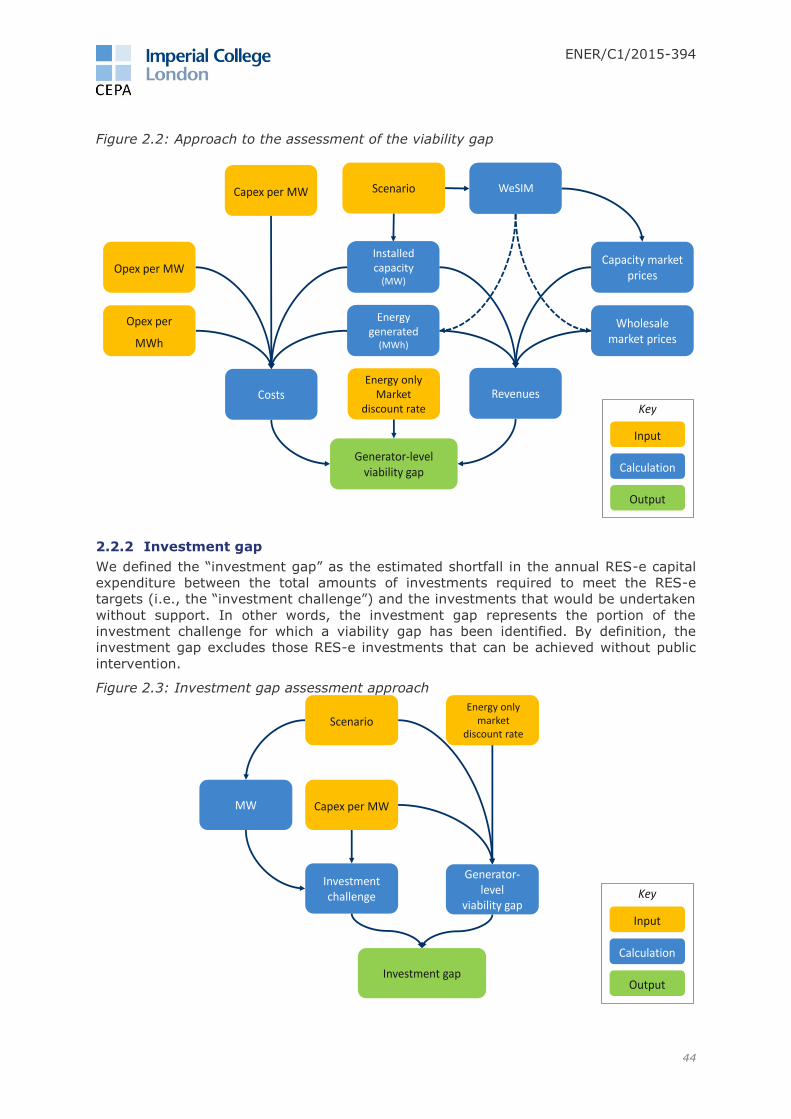
ENER/C1/2015-394

44

Figure 2.2: Approach to the assessment of the viability gap

2.2.2 Investment gap

We defined the “investment gap” as the estimated shortfall in the annual RES-e capital

expenditure between the total amounts of investments required to meet the RES-e

targets (i.e., the “investment challenge”) and the investments that would be undertaken

without support. In other words, the investment gap represents the portion of the

investment challenge for which a viability gap has been identified. By definition, the

investment gap excludes those RES-e investments that can be achieved without public

intervention.

Figure 2.3: Investment gap assessment approach



Discount rate

EOM only

MWh

Scenario


MW

Costs Revenues


WeSimCapex per MW

Opex per MW

Opex per

MWh

Output

Calculation

Input

Key

Installed capacity

(MW)

Energy generated

(MWh)

WeSIM



Discount rate

EOM only

MWh

Scenario


MW

Costs Revenues


WeSimCapex per MW

Opex per MW

Opex per

MWh

Output

Calculation

Input

Key

Energy only Market

discount rate

Discount rate

EOM only

MW Capex per MW

Investment challenge

Investment gap

Scenario

Generator-level

viability gap

Output

Calculation

Input

Key



Discount rate

EOM only

MWh

Scenario


MW

Costs Revenues


WeSimCapex per MW

Opex per MW

Opex per

MWh

Output

Calculation

Input

Key

Energy only market

discount rate

ENER/C1/2015-394

45

2.2.3 Funding gap

We estimate the annual “funding gap” as the cost of support required to bridge the

investment gap for a set of support options. This allows us to identify which options can

meet the respective investment challenge with the least amount of support, as well as

the relative margins between them.

Figure 2.4: Funding gap assessment approach

It is important to note that the findings from the above analysis are the product of the

assumptions made, and incorporate assumptions on the policy reforms that may alter

the functioning of the internal electricity market. All scenarios considered in this study

included some degree of market reform. The purpose of this analysis was not to assess

the relative merits of the alternative scenarios per se, but to analyse RES-e viability

under each scenario. All of our findings of generator viability or funding gaps assume

that the market reforms assumed under each scenario are successfully implemented.

We also note that the generator viability analysis did not include the cost to generators

of accessing the electricity transmission or distribution networks. Where charges for the

use of network infrastructure are recovered directly from generators, they would be an

additional cost, which must be recovered above and beyond the operating and capital

expenditure considered in this study. If transmission and distribution costs were

recovered through cost-reflective charges, investors would factor them into their

investment decisions when considering the viability of a potential project, and would

have an adequate incentive to operate their RES-e projects from locations where they

would impose the lowest cost on the system. Since cost-reflective network charges are

likely to be location- and project-specific, the level of detail incorporated into WeSIM was

insufficient for an explicit modelling of these decisions.

Consistent with the market modelling in WeSIM, many of the key inputs to the model,

such as MW installed, operating costs and capital costs, are adapted from PRIMES, using

guidance from the Commission. Discount rates used to assess viability gaps were

estimated by CEPA, and informed by input from an investor workshop held in Brussels in

June 2016. Further information on this analysis is provided in Section 5.1, with

information regarding the investor workshop provided in Section 4.2.1.

Scenario

Cost of supportby support option

Discount rateby support option

Viability gapby support

option

Marginal RES viability gap

Support level

MWh

Geog. scope

MWh eligible for support

Discount rateEOM only

Viability gapEOM only

Output

Calculation

Input

Key

Energy generated

(MWh)



Discount rate

EOM only

MWh

Scenario


MW

Costs Revenues


WeSimCapex per MW

Opex per MW

Opex per

MWh

Output

Calculation

Input

Key

Energy only market

discount rate

Support option discount rate

Geographical scope

ENER/C1/2015-394

46

2.3 Policy options for RES-e support

If the objective of RES-e targets is to decarbonise the electricity sector, then the

theoretical first best option is to internalise carbon costs into electricity prices using a

single policy instrument, such as the EU ETS. However, given the scale of the investment

challenge and investors’ scepticism regarding the ETS—in particular the perception that

carbon prices will not be sufficiently high to make RES-e viable—we believe that

additional policy instruments will be needed to ensure that the market provides the

necessary investments.

In this study, we applied the following guiding principles for identifying and assessing

policy options for RES-e support:

the option must be capable of attracting the required amount of RES-e

investment to meet decarbonisation goals;

RES-e targets are met at least social cost;

the option must be compatible with EU energy policy up to 2030 and beyond;

simplicity; and

only provide support to RES-e technologies that require financial support because

their market revenues are insufficient.

More detailed discussion of the policy options analysed in this study is contained in

Section 4.

ENER/C1/2015-394

47

3 Possible future RES-e and electricity market developments

In this section of the report, we first discuss possible market developments through

2050 that could have important financial implications for RES-e. These developments

provide the motivation and the rationale for the scenarios that we developed for this

study. In the latter half of the section, we describe our scenarios in more detail,

including the main assumptions behind each of them.

3.1 Possible future market conditions for RES-e

An energy-only market (EOM) is seen by many as the appropriate design for electricity

markets because it could potentially avoid the need for regulatory interventions. In an

EOM, RES-e would primarily rely on energy market revenues to recover their costs, with

a significant portion of annual revenues being earned during a few hours of scarcity.

Therefore, it is crucial to ensure that electricity is priced accurately to reflect the true

value of scarcity when electricity is in short supply. If scarcity is not priced accurately, a

significant portion of market revenues could be at risk.

Some MS have already deviated from the EOM market design by implementing or

planning to implement a Capacity Remuneration Mechanism (CRM). Some view these

developments with concern, arguing that CRMs may negatively impact RES-e.

Other developments, such as the evolution of carbon prices, will also be important for

RES-e. The EU ETS is perceived by many market participants to be a source of

uncertainty, since carbon prices will have to be a key driver of future decarbonisation,

notably via the incentives they will provide through higher electricity prices, and thus

RES-e market revenues.

Furthermore, increasing RES-e penetration will necessitate measures to make the power

system more flexible. This can be done by increasing demand side flexibility (e.g.,

developing demand side response, dynamic pricing, etc.) or adding supply side flexibility

(e.g., installing more flexible conventional generators or adding new technologies, such

as storage devices), or both. On one hand, increasing supply and demand side flexibility

is beneficial for RES-e because it allows the integration of higher amounts of RES-e

capacity. On the other hand, it may have some countervailing effects (e.g., it may

dampen prices during scarcity hours).

Enhancing interconnectivity across the EU is important for RES-e, since a more

interconnected and integrated market allows for a better integration of RES-e. It also

allows for a more efficient allocation of RES-e capacity across the EU, to take advantage

of the best potential sites for RES-e.

Lastly, energy efficiency measures may also impact RES-e market revenues. While

energy efficiency is an important tool to meet decarbonisation targets, all else equal, it

reduces demand and thus market revenues for RES-e.

Next, we discuss these developments in more detail. First, Section 3.1.1 briefly discusses

EOMs. This is followed by a discussion of introducing CRMs, and their implications for

RES-e, in Section 3.1.2. Possible developments related to the EU ETS are described in

Section 3.1.3. Lastly, other possible developments are covered in Section 3.1.4.

3.1.1 Energy-only market (EOM)

In an EOM, generators receive the majority of their revenues from the sale of energy, in

addition to other revenues they may derive from the sale of system services (e.g.,

frequency response), but they are not remunerated through capacity payments. Thus,

generators in an EOM recover their fixed costs primarily through the infra-marginal rents

when the market price exceeds their own variable costs, as well as scarcity rents they

ENER/C1/2015-394

48

receive during hours when prices exceed the variable cost of every generator in the

market, including the marginal generator.

The marginal generator is the most expensive generator in the supply stack. This

generator typically runs for a relatively small number of hours each year, and

recuperates its fixed costs by generating in those hours when market prices rise to

above its marginal cost of generating. In order for such spikes to occur, prices need to

reflect scarcity during periods of low security margins. In theory, if the supply stack is

exhausted, the electricity price should be able to rise up to the value of lost load (VoLL),

which is the value placed on unanticipated demand interruptions by demand. This is

usually estimated to be in the thousands of euros.18

For investment signals to be strong enough to actually deliver new capacity in an EOM,

investors must have confidence in the market to produce infra-marginal rents. For

generators at the top of the supply stack this means producing scarcity rents. From the

perspective of RES-e, scarcity prices lead to higher revenues than would be the case if

scarcity was not reflected in prices. Thus, all else equal, scarcity prices should increase

market revenues. Dispatchability also becomes important in an EOM, since dispatchable

RES-e technologies, such as biomass, have a greater ability to capture scarcity rents

than non-dispatchable generators, which include several RES-e technologies.

3.1.2 Capacity Remuneration Mechanisms

While Capacity Remuneration Mechanisms (CRMs) are currently subject of an intense

debate, it is likely that, at least in the medium term, they are likely to be part of the

European electricity market landscape. Figure 3.1 below summarises the current status

of CRMs in the EU and other markets around the world. There is a clear tendency

towards more, not fewer, capacity markets, therefore it is important to assess the

implications of this trend for RES-e development.

18 For example, recent VOLL estimates for the UK range from about £1,600/MWh to £44,000/MWh. References: London Economics, The Value of Lost Load (VoLL) for electricity in Great Britain (July 2013): https://www.gov.uk/government/uploads/system/uploads/attachment_data/file/224028/value_lost_load_elect

ricty_gb.pdf; RAEng, Counting the cost: the economic and social costs of electricity shortfalls in the UK (November 2014): http://www.raeng.org.uk/publications/reports/counting-the-cost.

https://www.gov.uk/government/uploads/system/uploads/attachment_data/file/224028/value_lost_load_electricty_gb.pdf


http://www.raeng.org.uk/publications/reports/counting-the-cost

ENER/C1/2015-394

49

Figure 3.1: Existing and planned CRMs in the EU and other markets

Source: EY, Utilities Unbundled, Issue 18, February 2015, Figure 1

The concern regarding these developments is that the implementation of CRMs across

the EU in a non-harmonised manner may disrupt the process of creating a competitive,

fully integrated Internal Electricity Market (IEM). Examining these issues was beyond the

scope of our study, but in order to determine the most appropriate forms of renewable

support schemes, we considered it important to study a scenario which includes CRMs.

The main purpose of our CRM sensitivity scenario was to study the potential impacts on

the RES-e viability gap of introducing national and regional/EU-wide capacity

remuneration mechanisms. In all other scenarios, we assumed an EOM where energy

prices are the only source of market revenues for RES-e.

In an EOM, generators’ revenues primarily consist of wholesale market revenues from

the sale of energy, which is a direct function of energy generated. The presence of a

CRM can significantly change the wholesale market revenues and the viability gap of

RES-e because capacity mechanisms reward generators not for energy output, but for

guaranteeing availability (firm capacity) during reliability events, especially during those

periods when generating capacity to serve demand is limited. Since RES-e generators

generally have a lower ability to guarantee firm capacity than conventional generators,

capacity payments as a source of revenue tend to be less significant for RES-e.

Furthermore, capacity payments for RES-e are not likely to offset the decrease in energy

market revenues, and thus the introduction of a CRM may leave them worse off.

In theory, CRMs are not needed to ensure reliability. In an EOM, the wholesale market

price of energy plays a key role in ensuring reliability; by rationing scarce supplies in the

short run, and by incentivising new entry, when needed, in the long run. When supplies

ENER/C1/2015-394

50

are scarce, the wholesale energy price will rise to scarcity price levels. These are prices

that exceed the short-run marginal cost of the highest-cost generation because the

generator supply stack is fully exhausted, and are set by demand that is willing to be

interrupted, based on their willingness to be curtailed, expressed by the VoLL.

In practice, the EOM design may be perceived to be insufficient to ensure the desired

level of reliability because:

Interventions, such as price caps19, prevent market prices from reflecting the full

value of scarcity.

There may be alternating periods of relatively high and relatively low reliability,

due to the nature of investment cycles, which regulators may not find tenable.

Investors may find it too risky to invest in peaking capacity that earns most of its

revenues during a few hours a year, or even less frequently.

Demand side response, which is a crucial element of successful EOM, is currently

not sufficiently developed and its future uptake may be slow.

In light of these problems related to the EOM, some MS may find it more tenable and

appropriate to provide the scarcity rents an EOM would provide in the form of steady and

predictable capacity payments. Our CRM scenarios were developed with these

considerations in mind. More detail on our approach to modelling CRMs can be found in

Annex G.

3.1.3 EU Emissions Trading System

The EU ETS is a major pillar of EU climate policy. Its main goals are to restrict the total

level of emissions across Europe, and to incentivise participants to invest in cleaner

technology. In an EOM, ETS is crucial, as it has a direct impact on wholesale energy

prices, and therefore revenues received by RES-e. If ETS prices are too low, prices and

investment signals for low carbon RES-e technologies will be muted.

The ETS covers power plants, energy-intensive industries and commercial aviation

across the 28 EU MS and three non-EU countries (Iceland, Norway and Liechtenstein).

The cap-and-trade system sets a limit on the overall level of CO2 and other greenhouse

gas emissions. The EU ETS design has evolved since its introduction in 2005. Currently,

EU-wide emissions targets are set by the Commission, and allowances are allocated to

each participating country. Initially, ETS allowances, representing one tonne of CO2

each, were either allocated to companies for free or through a competitive auction. The

default allocation method is now auctioning. After the initial allocation process,

participants can trade their allowances in secondary markets.

The allocation of ETS allowances has been organised into four phases:

Phase 1 – most allowances were allocated freely. The over-provision of

allowances resulted in near zero prices.

Phase 2 – oversupply of credits combined with reduced output from the global

recession led to low carbon prices (persistently below €10/ tonne in 2012).

Phase 3 – the current phase. Current ETS futures contracts for delivery in

December 2016 trade at around €6/ tonne CO2.

Phase 4 – to be implemented from 2020, will reduce the emissions cap and

volume of allowances more rapidly, which should increase carbon prices. This will

be helped by mechanisms implemented in the course of Phase 3, such as the

Market Stability Reserve (MSR).

19 Although the theoretical EOM design does not include price caps, in practice price caps, albeit set at relatively high levels, are often incorporated.

ENER/C1/2015-394

51

It is widely recognised that oversupply of ETS allowances has led to the historically low

ETS prices, which has prompted the development of the MSR and the back-loading of

allowances in Phase 3. Since the supply of allowances is set administratively, there was

an oversupply of allowances such that demand was less than supply for allowances,

resulting in low carbon prices. The historically low ETS prices have meant that the

incentive to invest in low carbon technologies, including RES-e, has been dampened. At

present, ETS remains one of the main sources of uncertainty, since investors may not

perceive commitments to high carbon prices in the future as credible policy.

3.1.4 Other possible developments

As the EU progresses towards its long-term goal of decarbonisation, there are a number

of other possible developments in the electricity system, as well as in the wider

economy, that could influence the attractiveness of RES-e investments. Developments in

system flexibility are one such area, which is considered to be vital for achieving high

levels of RES-e penetration. IRENA (2015) describes four interrelated sources providing

system flexibility:20

1. flexible dispatchable generators (primarily, gas-fired OCGTs and CCGTs, and

hydro generators, including pumped storage);

2. interconnection (i.e., ‘leaning’ on neighbouring systems to manage variable

generation);

3. demand side response (DSR); and

4. new energy storage (both conventional, such as pumped storage, as well as new

types of storage devices, such as batteries).

These sources of flexibility are likely to become more important as the share of

intermittent generation in the system increases. In their 2015 Scenario Outlook and

Adequacy Forecast (SOAF),21 ENTSO-E has identified countries across Europe that are at

risk of having to curtail RES-e generators due to inadequate system flexibility (shown in

the rightmost three columns of Figure 3.2 below).

20 IRENA (2015) 21 ENTSO-E (2015)

ENER/C1/2015-394

52

Figure 3.2: RES-e penetration and curtailment risk

Source: ENTSO-E SOAF 2015, Table 5.4.1

It is apparent that the Commission is prioritising flexibility alongside RES-e integration in

the new energy market design consultation that has a vision to ‘…fully integrate all

market players – including flexible demand, energy service providers and renewables.’

Flexibility through interconnection has also clearly been prioritised by the Commission’s

2030 target to have 15 percent interconnection across Europe, for which they have

recently set up an expert working group.22

New storage technologies, such as electric vehicles and in-home batteries, have the

potential to become more widespread at the distribution level. However, it is currently

difficult to forecast how much distribution-level storage is realisable, given the

uncertainties around future costs. For utility-scale storage, pumped hydro storage (PHS)

22 https://ec.europa.eu/energy/en/news/new-expert-group-electricity-interconnection-targets-call-applications-deadline-extended

https://ec.europa.eu/energy/en/news/new-expert-group-electricity-interconnection-targets-call-applications-deadline-extended

https://ec.europa.eu/energy/en/news/new-expert-group-electricity-interconnection-targets-call-applications-deadline-extended

ENER/C1/2015-394

53

is by far the most mature technology, but its growth is limited by geography,23 and is

thus not expected to significantly enhance system flexibility.

While flexibility is important from a system operations perspective, flexibility can also

both positively and negatively impact individual RES-e generators financially. In

particular, DSR can take the form of peak shaving or demand shifting. Peak shaving

lowers peak prices without affecting off-peak prices, and thus has a negative impact on

RES-e that generate during peak periods. Demand shifting, on the other hand, reduces

demand in peak periods and raises demand in off-peak periods, resulting in, all else

equal, lower prices in peak periods and higher prices in off-peak periods. This may

benefit RES-e that tend to generate mostly in off-peak periods, since higher demand in

those periods will result in higher prices, while they are not affected by the reduction in

peak-period prices. In this respect, storage devices have a similar impact as demand

shifting. Overall, the impact of DSR and storage on individual RES-e revenues depends

on their generation pattern and the net impact of the two countervailing effects

described above.

In terms of achieving decarbonisation targets, energy efficiency investments have also

been prioritised, as embodied in the Commission’s Energy Efficiency Directive. Currently,

energy efficiency targets are set at 27 percent by 2030. For RES-e, higher energy

efficiency would lower overall demand for electricity. So, while energy efficiency is

desirable from a decarbonisation perspective, it could potentially be harmful to RES-e

revenues.

3.2 Modelled scenarios and sensitivities

To assess how different support options are likely to perform under a variety of potential

future states of the world, we developed multiple scenarios, for which RES-e market

revenues were simulated. These scenarios are based on the PRIMES scenarios used by

the Commission in preparation of its 2016's Energy Union-related impact assessments.

They were designed to assess the impact of key drivers on RES-e revenues, namely:

electricity demand;

energy efficiency;

RES-e penetration;

interconnection capacity;

demand side flexibility;

capacity remuneration mechanisms; and

preferential market rules.

The key drivers listed above were incorporated into the five scenarios and six

sensitivities. We define scenarios as those, in which more than one parameter changes

compared to the base case (WeSIM RES27/EE27). In contrast, sensitivities represent a

change in a single parameter, compared to the base case. These are summarised in

Figure 3.3 and Table 3.1 below.

23 The Joint Research Council estimated the greatest potential for PHS in UK, Spain, Italy and Austria. Source: JRC (2013a)

ENER/C1/2015-394

54

Figure 3.3: Scenarios and sensitivities

Source: CEPA

Table 3.1: Summary of modelled scenarios and sensitivities


Main scenarios

1 WeSIM RES27/EE27 Based on the PRIMES EUCO27 scenario, which assumes that the 27 percent energy efficiency and the 27 percent RES-e targets are met by 2030. This serves as the baseline scenario.

2 WeSIM RES27/EE30 Based on the PRIMES EUCO30 scenario, which assumes that a 30 percent energy efficiency and a 27 percent RES-e penetration level is achieved by 2030.

3 WeSIM RES27/EE

Pessimistic

A scenario with a combination of lower levels of demand side response, interconnection, carbon prices and energy efficiency than the baseline scenario. The 27 percent RES-e target is still achieved

by 2030.

4 WeSIM Ref Based on the PRIMES Reference Scenario.

5 WeSIM RES30/EE30 Based on PRIMES RES30/30 scenario. Assumes 30 percent energy

efficiency and 30 percent RES-e penetration by 2030.

Sensitivities on the baseline scenario (WeSIM RES27/EE27)

1 Lower ETS Carbon prices are lower in 2040 and 2050.

2 National CRM Payments provided for capacity available during scarcity periods

under national capacity remuneration mechanisms.

3 No pref rules Preferential market rules (e.g., priority dispatch for biomass generators) removed after 2020.

4 Imperfect foresight Investors only have limited certainty over future carbon prices.

5 WACC+ Assumes a mark-up of 100 and 200 basis points, respectively, on top of the baseline discount rate for projects.

6 Low offshore cost Lower offshore wind capex from 2020.

Next, we discuss each scenario, including the rationale behind them, as well as our key

assumptions.

WeSIM EE27

WeSIM EE27

Pessimistic

WeSIM Ref

WeSIM EE30

WeSIM 30/30

National CRMs

Imperfect foresight of carbon prices

Removal of preferential market

rules

Two WACC sensitivities

Scenarios Sensitivities

Lower ETS

Offshore sensitivity

ENER/C1/2015-394

55

While each scenario differs in at least one material aspect, they all assume a fully-

functioning internal electricity market. All the scenarios, apart from the CRM sensitivity,

share the overarching assumption that RES-e revenues consist purely of EOM revenues.

We describe further below how we relax this assumption to account for the possibility of

introducing CRMs.

Common assumptions for the modelled scenarios are set out in the Table 3.2 below.

Table 3.2: Common assumptions for all scenarios

Assumption Description

Hourly demand profiles Forecasts of hourly demand profiles were taken from ENTSO-E’s

TNYDP 2016, Vision 3, for 2020, 2025 and 2030. We assumed

that hourly demand profiles were unchanged after 2030.

Generation capacity for non-

EU 28 states

Projected installed capacity was taken from ENTSO-E’s Ten-Year

Network Development Plan (TYNDP) 2016 and National Renewable

Energy Action Plans. It was assumed to be unchanged after 2030.

Fuel prices Coal, oil and gas price projections were taken from the analysis

performed in the EU Reference Scenario 2016. Parsons

Brinkerhoff supplied biomass forecasts and uranium prices were

taken from ENTSO-E’s TYNDP 2016.

Technology costs (RES-e and

conventional generation)

Parsons Brinkerhoff provided RES-e variable O&M costs.

Conventional technology variable O&M and fixed costs were

provided by Imperial College London. Capex costs were adapted

from PRIMES for both RES-e and conventional technologies.

DSR supply curves Supply curves for curtailable DSR were developed using the

methodology described in Annex F.

Policy targets to 2020 Each scenario assumes that policy targets for 2020, as set out in

MS NREAPs, are achieved by 2020 (i.e., first year of simulation).

Source: CEPA

Next, we briefly discuss the differences in key parameters across scenarios.

3.2.1 Electricity demand and energy efficiency

Energy efficiency improvements influence the demand for electricity. All else equal,

higher levels of energy efficiency should lead to lower levels of electricity consumption,

and therefore lower wholesale electricity prices. Energy efficiency targets are measured

as a reduction in primary energy demand compared to a ‘business as usual’ scenario,

and are currently set at 20 percent for 2020 and 27 percent for 2030.24 All of our

scenarios assumed that the 2020 energy efficiency targets would be met, but the level of

energy efficiency achieved by 2030 varied by scenario.

In addition to energy efficiency, the PRIMES Reference scenario—used to calibrate the

WeSIM RES27/EE Pessimistic and WeSIM Ref scenarios—included differences in other

factors that affect electricity demand, such as the penetration of electric vehicles.

Greater electric vehicle penetration would increase electricity demand, all else equal,

pushing electricity prices up, while energy efficiency improvements would push prices

down. The impact of energy efficiency and electric vehicles are both reflected in the total

demand for electricity, shown in the figure below. Note that the WeSIM Ref and WeSIM

RES27/EE Pessimistic scenarios have the same level of demand.

24 For related documents see Commission’s 2030 Energy Strategy. (link)

http://ec.europa.eu/energy/en/topics/energy-strategy/2030-energy-strategy

ENER/C1/2015-394

56

Figure 3.4: Final electricity demand plus transmission losses in the EU by scenario

Source: CEPA analysis, based on PRIMES

3.2.2 RES-e penetration

Most renewable generators, except for biomass, have zero (or near-zero) marginal costs,

and are usually “price takers” in the wholesale market. Thus, with higher penetration of

RES-e, we would expect to see average prices, and therefore revenues, decline as they

replace more expensive conventional generators.25 The hypothesis is therefore that

renewables cannibalise their own revenues as deployment increases.

Currently, the EU’s 2030 Energy Strategy sets a target of 27 percent for the share of

primary energy consumption to be supplied by renewable sources. In terms of electricity

demand and RES-e, this has been projected to translate into approximately 48 percent

of electricity demand (plus losses) being supplied by renewable generators across the EU

in the baseline scenario (WeSIM RES27/EE27). Our scenarios flex this assumption,

testing states of the world where (i) RES-e equals, (ii) is less than or (iii) is more than

the amount assumed in the baseline scenario, as summarised in Figure 3.5 below.

WeSIM RES27/EE27 and the WeSIM RES27/EE Pessimistic scenario achieve the same

RES-e penetration rate in all years (by construction).

25 This is referred to as the ‘cannibalisation effect’. We plan to present the Commission the magnitude of this effect for our scenarios and sensitivities in the first draft of our final report.

2,000

2,500

3,000

3,500

4,000

4,500

2015 2020 2025 2030 2035 2040 2045 2050

Fin

al e

lect

rici

ty d

eman

d p

lus

loss

es

(TW

h p

er

an

nu

m)

WeSIM RES27/EE27

WeSIM RES27/EE30


WeSIM Ref

WeSIM RES30/EE30

ENER/C1/2015-394

57

Figure 3.5: RES-e share of final electricity demand plus losses in the EU

Source: CEPA

3.2.3 Interconnection capacity

We assumed the same baseline level of interconnection capacity in all scenarios except

for the WeSIM RES27/EE Pessimistic scenario, which is assumed to have a lower level of

interconnection. As a baseline, we used projections of interconnection capacity from

ENTSO-E’s TYNDP 2016, up to 2030. However, as part of WeSIM’s optimisation process,

the model endogenously adds incremental interconnection capacity, as long as it is

efficient to do so from a whole system cost perspective, taking into account the cost of

all other alternatives. After 2030, we did not assume any new particular interconnectors

would be built, and left WeSIM’s optimisation process to endogenously add capacity.

In the WeSIM RES27/EE Pessimistic scenario, we assumed that the baseline level of

interconnection up to 2030 did not include those ‘Projects of Common Interest’ (PCIs)

identified by ENTSO-E that are expected to become operational between 2020 and

2030.26 For all other scenarios, we assumed that all PCIs would be built. Even though the

WeSIM RES27/EE Pessimistic scenario started with less interconnection capacity than the

other scenarios, WeSIM’s optimisation algorithm yielded additional capacity, with the net

result that the WeSIM RES27/EE Pessimistic scenario had slightly more interconnection

capacity than the other scenarios in 2050.

3.2.4 Demand side flexibility

A key feature of all scenarios is the provision of system flexibility through DSR, which is

part of overall system flexibility also provided from other sources, such as

interconnection, flexible generation and storage. DSR has been identified as a key

feature in the Commission’s Roadmap 2050 and the move towards a decarbonised

economy.

We modelled two types of DSR: shiftable demand and curtailable demand. Our approach

to modelling was informed by what has been observed in markets where demand

resources are much more developed and integrated into the wholesale market (e.g., PJM

26 ENTSO-E (2016)

0%

10%

20%

30%

40%

50%

60%

70%

80%

90%

100%

2015 2020 2025 2030 2035 2040 2045 2050

RE

S-e

gen

erat

ion

(% o

f ele

ctri

city

dem

and

)

WeSIM RES27/EE27

WeSIM RES27/EE30


WeSIM Ref

WeSIM RES30/EE30

ENER/C1/2015-394

58

market in the US), as well as past studies on achievable potential of DSR. We then

disaggregated the total achievable potential into shiftable demand resources and

curtailable demand resources.

Next, we used projections of system flexibility, based on PRIMES, to identify those

countries that would have the greatest need for additional flexibility through DSR in the

future. We assumed that countries with a high need for additional flexibility would

implement policies to encourage the development of DSR to reach the maximum

achievable level of DSR, which we set at ten percent of peak load. Our analysis also

considered the speed at which countries would be able to increase DSR penetration, and

whether DSR penetration would be limited by structural factor—such as the small size of

the industrial sector—given that a large proportion of currently observed DSR has been

achieved to date from industry, manufacturing and mining.

The outcome of our analysis is presented in the map below, which shows the maximum

achievable level of DSR in different MS. More detail on our approach to modelling and

implementing DSR in our electricity market modelling can be found in Annex F.

Figure 3.6: Assumed DSR penetration


3.2.5 Capacity remuneration mechanisms

The purpose of the CRM sensitivity scenario was to study the potential impacts on the

RES-e viability gap of introducing national and regional/ EU-wide CRMs. We consider that

the main rationale for introducing a CRM would be to ensure the same level of reliability

as would be provided by an efficient EOM (i.e., one free of distortions), rather than to

increase the level of reliability (i.e., procure more capacity).

For each MS in each modelled year, we determined the capacity payments for RES-e

according to the following steps:

Legend Shiftable CurtailableNot modelled - -Low DSR penetration 3% 2%Medium DSR penetration 5% 3%High DSR penetration 6% 4%

ENER/C1/2015-394

59

1. Determine scarcity pricing hours from the baseline EOM scenario (WeSIM

RES27/EE27)—these hours are those where loss of load probability (LOLP) is

greater than the assumed security standard (LOLE of 3 hours/year).27

2. Calculate total scarcity rents from the EOM (WeSIM RES27/EE27) scenario—

since the CRM is assumed to transform uncertain scarcity rents into steady

capacity payments, it is assumed that the two will be equal.

3. Determine capacity credit of each capacity resource—for each resource type,

determine the LOLP-weighted capacity factor during scarcity events in the EOM

scenario. Installed capacity of each resources type is de-rated by this factor.

4. Determine capacity price in terms of €/MW-year—this is determined by

dividing the total amount determined in Step 2 by the total de-rated capacity

(available in the national market).

5. Determine capacity revenues of each type of RES-e—capacity revenues are

calculated as the product of capacity price (€/MW-year) and the de-rated

capacity (MW).

6. Recalculate RES-e viability gap.

We assume that only those MS that experience reliability or scarcity events in the EOM

scenario implement a national CRM.

3.2.6 Preferential market rules

Priority dispatch is a market access rule, which places an obligation on Transmission

System Operators (TSOs) to schedule and dispatch RES-e generators ahead of all other

types of generation. In other words, priority dispatch artificially pushes some RES-e

generators down the merit order, displacing other lower-cost conventional generators.

The purpose of priority dispatch is to provide certainty to renewable generators that they

will be able to sell electricity into the grid at all times (thus reducing volume risk), and to

enable a more rapid integration of RES-e generators into the power system.

Currently, priority dispatch is combined with other forms of support (e.g., feed-in tariffs

(FITs) and Contracts for Difference (CfDs) in the UK) that make it profitable to sell

electricity on the wholesale market at any price, even below marginal cost. Although

priority dispatch was implemented for all RES-e generators, it was material only for

those with non-zero marginal costs, namely biomass plants.

The allocation of rights for priority dispatch in the EU has been purely administrative and

is set out by the Renewable Energy Directive, which states:

“Member States shall ensure that when dispatching electricity generating

installations, transmission system operators shall give priority to generating

installations using renewable energy sources.”28

However, it is also clearly set out in the legislation that in the event that renewable

generators participate in wholesale markets, the Directive does not require MS to

provide support, or to make purchase obligations, for renewable electricity.29

The baseline assumption for our scenarios is that priority dispatch for biomass

generators would continue to be implemented across Europe, and would be combined

with the RES-e support options. However, priority dispatch has important implications for

the overall economic efficiency of the electricity system since it distorts the merit order,

and therefore dispatch of generators. Consequently, we tested the impact of removing

priority dispatch on RES-e revenues.

27 LOLP is calculated in WeSIM. 28 2009/28/EC, paragraph 2(c) 29 2009/28/EC, paragraph 61

ENER/C1/2015-394

60

3.2.7 Investor foresight of carbon prices

As we describe in Annex A, WeSIM is a deterministic model that performs a least-cost

dispatch of generators across all of Europe, taking all inputs—including carbon prices—as

given. If investors accepted the prices simulated by WeSIM at face value, they would

effectively assume they have perfect foresight, without any considering any uncertainty

around the price projections. Since our other scenarios assumed that this would be the

case, the levelised cost of electricity (LCOE) estimates, and therefore viability gaps, do

not fully capture the role uncertainty plays in investment decisions.

Assuming perfect foresight of market revenues is not entirely realistic, since investors’

forecasts over long horizons will contain a high degree of uncertainty. Therefore, it is

reasonable to expect investors to be somewhat myopic regarding long-term revenue

forecasts. By this, we mean that investors are likely to be more certain about, and put

more weight on, short-term revenue projections than longer-term projections. This

effect goes beyond the discounting of future revenues.

Our initial modelling results indicated that high ETS prices, projected by PRIMES for 2040

and 2050, were the main drivers of the RES-e viability gaps. While there are other

elements of the wholesale price trajectory predicted by WeSIM (e.g., increased demand

from electric vehicles or changes in fossil fuel prices), we consider that ETS prices are

one of the most material drivers of future prices. ETS prices are also a component of

wholesale prices, which bears a large degree of policy risk, given its recent performance.

Going forward, investors may be sceptical about a dramatic increase in ETS prices, and

not consider ambitious ETS prices projections credible. Therefore, to capture investors’

myopia of long-term energy market revenues, we focused on future carbon prices.

Since WeSIM cannot explicitly capture uncertainty, we implemented investors' imperfect

foresight of carbon prices as a sensitivity scenario in the LCOE model. To do this, we

adjusted the wholesale market revenues received by RES-e generators in such a manner

that the ETS component of prices increases gradually over time, starting from the first

year of operation for any given capacity investment. It is difficult to accurately determine

the contribution of carbon costs to the total wholesale price in every hour. We therefore

used a less granular approach, taking revenues from the WeSIM RES27/EE27 scenario as

a baseline:

1. For each year, in each country, we determined the yearly average wholesale

electricity price;

2. For each year, in each country, we calculated the total carbon costs per MWh

by multiplying total annual emissions times the ETS price, and dividing by total

demand;

3. For an investment in year T, we divided the results of step 2 by the result of

step 1. This gives an approximate value for carbon content of prices in the year

of the initial investment;

4. For all years after T, we subtracted the result of step 2 from step 1, and added

the result of step 3. This strips out the carbon content from future years,

replacing it with the cost of carbon from the year of the initial investment;

5. Lastly, LCOE was recalculated using the new, adjusted, revenue stream.

This approach differentiates between revenues from carbon prices and revenues driven

by other market fundamentals. The imperfect foresight is continuous in the sense that

investors in each year take as given the prevailing ETS price, and assume that it remains

constant over the life of their project.

3.2.8 WACC and offshore sensitivities

Most scenarios and sensitivities in this study seek to examine how changes in wholesale

market revenues affect RES-e viability. However, the discount rates used by investors to

ENER/C1/2015-394

61

assess those revenues, as well as the costs they expect to incur, are also uncertain.

Therefore, we further tested the robustness of our findings by performing three

additional sensitivities on the WeSIM RES27/EE27 baseline scenario:

two alternative discount rate sensitivity scenarios; and

a sensitivity scenario on offshore wind costs.

The discount rate sensitivity scenarios test the impact of assumed discount rate values

on the viability of RES-e technologies. We modelled the impact of a 100 and a 200 basis

point increase in the discount rate across all RES-e technologies. These sensitivities

capture some of the uncertainty around the rate of return required by investors, and also

the extent to which macroeconomic shocks or gradual shifts over time might affect RES-

e.

With the deployment projected to significantly increase over time, offshore wind is one of

the main RES-e technologies that is projected to require support under range of

scenarios. There is, however, a significant degree of uncertainty around the potential for

technology learning and cost reductions in offshore wind. Therefore, we developed a

sensitivity scenario where offshore wind capex is assumed to be nine percent lower in

2020 and 37 percent lower in 2030 than the base case. These assumptions reflect the

cost reduction pathway presented in the recent industry forecast,30 which indicate a 20

percent learning rate resulting in faster costs reductions than in the base case. We

analysed the impact of lower offshore costs on the viability of offshore wind technology.

3.2.9 Cannibalisation effect

Numerous studies31 have found that the presence of a “cannibalisation effect”—which

reduces the market value of RES-e when overall renewable penetration increases—has a

negative impact on RES-e viability. As a result, there is an ongoing conflict between

learning rates reducing the costs of RES-e and the cannibalisation effect reducing the

value of RES-e. Using WeSIM modelling results we calculated the cannibalisation effect

for the three most widely deployed intermittent RES-e: solar, onshore wind and offshore

wind.

3.2.10 The market value of intermittent RES-e

The market value of intermittent RES-e is generally affected by three key technological

properties:

The uncertainty of output in combination with day-ahead trading means that

forecast errors have to be corrected at very short notice, which reduces their

market value.

There are geographic restrictions on where RES-e can be deployed, for example,

where sun and wind are in abundance. Unfortunately, these locations are not

often close to load centres, which reduces their market value.

The intermittency of RES-e generation can have a positive or negative impact on

market value depending on the market price at the time of generation.

Two opposing effects determine the market value of RES-e: the “correlation effect”, and

the cannibalisation effect.

If the generation profile of a RES-e installation is positively correlated with demand, then

it could receive a higher average price compared to, for example, a baseload

conventional generator. This is known as the correlation effect, and has been observed

at low RES-e penetration levels. For example, the average electricity spot price in

30 Wind Europe (2016) 31 Borenstein (2008); Schmalensee (2014); Green and Vasilakos (2012).

ENER/C1/2015-394

62

Germany in 2011 was €51/MWh, while solar power received an average price of

€56/MWh, simply because it often generated at times when demand was high.32

The cannibalisation effect occurs at high levels of low- or zero-marginal cost generation,

which puts downward pressure on the market price of electricity. This is especially the

case for intermittent RES-e, such as solar and wind power, as the output of these

generators is usually correlated within a geographic market. A priori, we would expect

the effect to be greater for solar power, because increasing the installed capacity of solar

is likely to have a greater impact on the solar generation-weighted average price than

adding wind capacity would have on the wind generation-weighted average price. This is

due to the fact that, on average, solar installations tend to generate electricity in a fewer

number of high-demand hours.

Empirical evidence from earlier studies suggests that since intermittent RES-e generation

started playing a significant role in the generation mix, the cannibalisation effect has

begun to dominate the correlation effect.33

To measure the net impact of these two effects on the market value of intermittent RES-

e, we estimated the value factor, defined as the ratio of the average generation-

weighted hourly electricity price for intermittent RES-e and the average hourly electricity

price. The value factor measures the relative price earned by intermittent RES-e to the

average price earned by all generators. The value factor effectively normalises the price

received by intermittent RES-e across all MS with different levels of RES-e penetration.

We can thus collate the value factors of a particular intermittent RES-e across countries

and across years, and analyse the relationship between the value factor and penetration

of intermittent RES-e. In this section we provide a summary of our results for Germany.

3.2.11 Empirical results

In this section we focus on the cannibalisation effect for offshore wind, onshore wind and

solar PV in Germany.

Figure 3.7 presents the relationship between the value factor and penetration rate for

the WeSIM RES27/EE27 scenario. Projections from PRIMES imply that in Germany the

penetration of solar PV34 will be 7.2 percent in 2020. We estimate a corresponding value

factor of 0.98. However, by 2050 Germany's solar PV’s penetration is projected to

increase to 14.6 percent, with the value factor dropping to 0.73. In other words, as the

penetration of solar PV increases by about seven percentage points, its value factor

decreases by approximately 26 percentage points. The negative relationship between the

penetration rate and value factor of offshore wind is also significant, with its value factor

decreasing from 0.92 in 2020 to 0.73 in 2050, as penetration increases from 15.9

percent to 21.9 percent. Overall, the cannibalisation effect is significant for both solar PV

and offshore wind, but appears to be strongest for solar PV. The relationship is the

weakest for onshore wind, with no evidence of the cannibalisation effect. This outcome is

as expected, given the fact that solar tends to generate in fewer hours of the day

compared to onshore and offshore wind.

32 Hirth (2013) 33 Ibid. 34 Measured as total solar generation (GWh) divided by final electricity demand (GWh).

ENER/C1/2015-394

63

Figure 3.7: The relationship between the value factor and penetration rate of offshore wind, onshore wind and solar PV in Germany (WeSIM RES27/EE27 scenario)


Figure 3.8 shows the relationship between the value factor and penetration rate of

offshore wind, onshore wind and solar PV in Germany for the WeSIM RES27/EE30

scenario. The findings are similar to WeSIM RES27/EE27, with the cannibalisation effect

appearing the strongest for solar PV and the weakest for onshore wind. However, the

cannibalisation effect is generally weaker across wind and solar compared to WeSIM

RES27/EE27. The value factor for solar PV decreases from 0.98 to 0.79, as solar

penetration increases from 7.1 percent to 15.4 percent. This rate of decrease in the solar

value factor between 2020 and 2050 is slightly lower than the corresponding figure for

WeSIM RES27/EE27. Similarly, the value factor of offshore wind decreases from 0.92 in

2020 to 0.79 in 2050, as offshore wind penetration increases from 5.6 percent to 20.8

percent. This relationship is significantly weaker than in the WeSIM RES27/EE27

scenario. The cannibalisation effect is the weakest for onshore wind, with no clear

negative relationship between the value factor and RES-e penetration. Overall the

cannibalisation effect remains significant for solar PV and offshore wind, but it is weaker

than in the WeSIM RES27/EE27 scenario.

ENER/C1/2015-394

64



Figure 3.9 presents the relationship between the value factor and penetration rate for

the WeSIM RES27/EE Pessimistic scenario. It is clear that the cannibalisation effect

witnessed in WeSIM RES27/EE27 and WeSIM RES27/EE30 scenarios is substantially

weaker in the WeSIM RES27/EE Pessimistic scenario. In fact, no clear negative

relationship is observable between RES-e penetration and the value factor.

Figure 3.9: The relationship between the value factor and penetration rate of offshore wind, onshore wind and solar PV in Germany (WeSIM RES27/EE Pessimistic scenario)


Figure 3.10 shows the relationship between the value factor and RES-e penetration rate

the WeSIM RES30/EE30 scenario. In this case, evidence of the cannibalisation effect is

very weak, with no clear identifiable relationship between RES-e penetration and the

value factor for solar PV, offshore wind or onshore wind.

ENER/C1/2015-394

65



Lastly, Figure 3.11 presents the relationship between the value factor and penetration

rate of offshore wind, onshore wind and solar PV in Germany for the WeSIM Ref

scenario. The cannibalisation effect for solar PV is significant in this scenario, with the

solar value factor decreasing from 0.99 to 0.84, as its penetration increases from 7.2

percent to 10.0 percent. However, the relationship is weak for offshore and onshore

wind, with no clear negative relationship between penetration rate and the value factor.

Figure 3.11: The relationship between the value factor and penetration rate of offshore wind, onshore wind and solar PV in Germany (WeSIM Ref scenario)


3.2.12 Summary

While some scenarios, such as WeSIM RES27/EE27, provide strong evidence of a

dominating cannibalisation effect, this outcome does not translate across to all scenarios.

ENER/C1/2015-394

66

In particular, the relationship is particularly weak for the WeSIM RES27/EE Pessimistic

scenario. Where evidence of the cannibalisation effect is significant, the effect appears to

be most significant for solar PV, and least significant for onshore wind. This is perhaps

expected, given the fact that solar PV tends to generate in fewer hours of the day,

compared with onshore and offshore wind. The magnitude of the cannibalisation effect

will have an impact on the viability of RES-e technologies, and by extension, on subsidy

requirements. In particular, if the cannibalisation effect outweighs the costs savings from

learning rates, then it may be necessary to increase RES-e support over time in order to

keep them viable.

3.3 Potential future scale of the investment challenge

As described in the previous sections, each scenario is associated with a specific

investment challenge, which corresponds to the total amount of RES-e capital

expenditure that is required to achieve the decarbonisation objectives. Since each

scenario entails different targets, the quantity and the mix of RES-e in each MS will

differ, thus resulting in different magnitudes of the investment challenge.

To give an indication of the extent to which RES-e support might be required under

different scenarios from 2020 to 2050, we summarise our analysis of the overall

investment challenge in absolute terms before presenting generator-level viability gaps.

3.3.1 Investment challenge

Figure 3.12 below presents estimates of the magnitude of the investment challenge, or

put differently, the required amount of annual capital expenditure in RES-e capacity in

billions of euros in the EU as a whole35 under the five scenarios introduced in Section

3.2:36

WeSIM RES27/EE27;

WeSIM RES27/EE30;

WeSIM RES27/EE Pessimistic;

WeSIM Ref; and

WeSIM RES30/EE30.

35 Associated electricity network investment is not included in these numbers. 36 Results for the sensitivities (ETS, Non-Priority Dispatch, Imperfect foresight, WACC sensitivity and Offshore sensitivity) are the same as WeSIM RES27/EE27 scenario.

ENER/C1/2015-394

67

Figure 3.12: Required annual RES-e capital expenditure in €bn in the EU, by scenario


The investment challenge between 2020 and 2030 is estimated to be around €25 billion

annually. This is forecast to double by 2035, and triple by 2045, peaking under the

WeSIM RES27/EE27 scenario at €90 billion per year. This illustrates the significant ramp

up in RES-e investments that will needed to be made after 2035 to achieve the 2050

decarbonisation targets.

The difference in the investment challenge between the scenarios is the most significant

before 2030, which is in line with the underlying definitions of the scenarios that

differentiates them based on the level of RES-e penetration of energy efficiency achieved

by 2030. The WeSIM RES30/EE30 scenario has the highest level of both RES-e

penetration and energy efficiency in 2030 (30 percent for each). Therefore there is a big

push in investment under that scenario before 2030, in particular between 2025 and

2030 when the level of annual investment is around €40 billion, twice as much as under

the WeSIM RES27/EE27 scenario. From 2040, the level of investment under the WeSIM

RES30/EE30 scenario tails off as the majority of the investment has been made before

2040. One of the drivers of this reduction is the decrease in offshore wind investment

from 2040. Net installed capacity in offshore wind under the WeSIM RES30/EE30

scenario is already 26 percent higher in 2040 than under the WeSIM RES27/EE27, and

therefore the level of investment falls in the following decade.

Similarly the level of investment under the WeSIM RES27/EE30 scenario that assumes

30 percent of RES-e penetration in 2030 is the second highest until 2030. The lowest

level of investment before 2030 is under the WeSIM Ref scenario that assumes the

lowest level of RES-e penetration across scenarios.

The investment challenge shown above encompasses all the RES-e projects in the EU

that need to be installed by 2050. Over this period, some projects will be viable based on

electricity market revenues alone. However, in a number of the scenarios that we

examined, many RES-e will continue to require additional support, without which it

would not be possible to meet the investment challenge presented in Figure 3.12.

0

10

20

30

40

50

60

70

80

90

100

2015 2020 2025 2030 2035 2040 2045 2050

Annual capex in €

bn (

2015 p

rices)

WeSIM RES27/EE27 WeSIM RES27/EE30

WeSIM RES27/EE Pessimistic WeSIM Ref

WeSIM RES30/EE30

ENER/C1/2015-394

68

3.3.2 Viability gap

To estimate the potential investment gap, we first examined the forecast revenues and

costs over the expected life of each RES-e technology to identify, in a binary manner,

whether there was a viability gap, such that investments required for meeting the

decarbonisation objectives would not go ahead on the basis of electricity market

revenues alone. We performed this analysis for eight technologies at five different points

in time between 2020 and 2050, using the five scenarios shown in Figure 3.12.

Clearly, a key driver of RES-e viability is the market price of electricity. Electricity prices

are driven by market fundamentals, such as variable operating costs, the generation

capacity mix, the generation profile of intermittent technologies, demand for electricity

and carbon prices. To provide some context to the viability gap results, we show the

estimated progression of average electricity prices across the modelled scenarios in

Figure 3.13 below.

Figure 3.13: Average EU electricity price – all scenarios (€/MWh, 2015 prices)


There is a clear upward trend in electricity prices in all scenarios, with prices between

scenarios starting to diverge only after 2030. This is driven by similar assumptions in the

earlier years across the scenarios, including assumptions about capacity mixes and

carbon prices.37 After 2030, simulated electricity prices significantly diverge, potentially

driven by differences in the following assumptions:

electricity demand;

demand side response;

capacity mix; and

carbon prices.

As we saw in Section 3.2.1, electricity demand is fairly similar across most years and

scenarios, except in the WeSIM Ref scenario and in 2030 for WeSIM RES27/ EE30 and

WeSIM RES30/EE30 scenarios when there is a dip in demand. While demand explains

some of the price differentials observed between scenarios, it is not the largest

contributor. DSR is also quite similar across scenarios, thus it is not a major driver of

price differentials either. Carbon prices, on the other hand, significantly differ in the

37 Generation profiles and variable operating costs do not vary by scenario. See Annex A for more detail on modelling assumptions.

0

20

40

60

80

100

120

140

160

180

200

2020 2025 2030 2040 2050

€ /

MW

h

WeSIM RES27/EE27 WeSIM RES27/EE30 WeSIM RES27/EE Pessimistic

WeSIM Ref WeSIM RES30/EE30

ENER/C1/2015-394

69

WeSIM Ref and WeSIM RES27/EE Pessimistic scenarios, compared to the other

scenarios. ETS prices are factored into wholesale prices by increasing the marginal cost

of carbon-emitting generators. While it is difficult to isolate the exact magnitude of the

impact of ETS prices, our low ETS price scenario sheds some light on it.38 Figure 3.14

below shows the average electricity price in the WeSIM RES27/EE27 and Low ETS

scenarios. In the latter, ETS prices were 36 percent lower in 2040 and 2050, compared

to the WeSIM RES27/EE27 scenario, which is reflected in lower electricity prices.

Figure 3.14: Average EU electricity price – WeSIM RES27/EE27 vs Lower ETS prices (€/

MWh)


ETS prices are thus clearly one of the main contributors to the price differentials, with

lower ETS prices leading to a reduction of between €10-20 per MWh in average prices

between 2040 and 2050. In addition, the capacity mix also plays a significant role in

explaining price differentials, as a result of the following differences between scenarios:

Different penetration and types of RES-e.

Different penetration of carbon emitting technologies (i.e., coal, gas, oil).

Different penetration of carbon capture and storage (CCS) technologies.

All of these factors interact with one another, as well as with the carbon price. Even with

increasing ETS prices it is possible for electricity prices to decrease. This may occur if, for

example, there is a significant increase in the penetration of CCS technology, which are

not impacted by the increase in the carbon price. The same can be said of increased

rates of RES-e penetration, which put a downward pressure on average prices. We

observe this in the WeSIM RES27/EE27 scenario when looking at average prices between

2040 and 2050. When comparing the WeSIM RES27/EE27 and WeSIM RES27/EE30

scenarios, capacity mix also plays a large part, particularly since we see lower

penetration of CCS and RES-e in the WeSIM RES27/EE30 scenario, which contributes to

higher average prices.

The particular set of assumptions made for each scenario determines the electricity

prices, RES-e revenues, and the viability gap. Our estimates of the viability gap for RES-

e under the various scenarios are discussed next.

38 Note that the Lower ETS price scenario can be interpreted as one where investors expect a low ETS price in

the future. In contrast, in the Imperfect foresight regarding ETS price scenario, investors expect that future ETS prices will be in line with current prevailing prices, which may be high, low or in between.

0

20

40

60

80

100

120

140

160

2020 2025 2030 2040 2050

€ /

MW

h

WeSIM RES27/EE27 Lower ETS

ENER/C1/2015-394

70

2020 scenarios

Figure 3.15 and Figure 3.16 below present our findings of the viability gap by

technology, MS and scenario in 2020, expressed as the minimum additional revenue per

MWh needed over the life of the generator to be viable. Each mark plotted on the chart

represents a RES-e technology in a given country.39 Marks above the horizontal axis

indicate a positive viability gap, and therefore represent RES-e in MS where additional

support may be required. Marks below the horizontal axis represent RES-e technologies

and countries where electricity market revenues might be sufficient on their own, and

further intervention may not be necessary.

Across all technologies, the WeSIM RES27/EE Pessimistic scenario results in relatively

higher viability gaps on average, driven mostly by the comparatively low wholesale

prices from 2030 to 2040. These relatively low prices are likely the result of much lower

ETS prices. By comparison, the WeSIM Ref scenario also has low ETS prices (pushing

wholesale prices down), but has lower RES-e penetration, and therefore less

cannibalisation of revenues. Generally speaking, for RES-e projects built in 2020

wholesale market revenues are not yet high enough to support RES-e alone, the notable

exceptions being run-of-river (ROR) hydro, onshore wind and solar PV in some MS.

39 Note that not all RES-e technologies are included for every country, partly because some countries do not have the potential (e.g., landlocked countries cannot have offshore wind), and also because some RES-e

technologies in certain countries are not part of the least-cost RES-e mix required to meet the targets, as projected by PRIMES.

ENER/C1/2015-394

71

Figure 3.15: Viability gap in 2020 by scenario for biomass, geothermal, hydro ROR and

hydro reservoir40


40 Please note that no data points are shown for geothermal in Figure 3.15 as no new geothermal capacity was included in the investment challenge for 2020.

-100

-50

0

50

100

150

200

250

300

WeS

IM R

ES2

7/EE

27

WeS

IM R

ES2

7/EE

30

WeS

IM R

ES2

7/EE

Pes

sim

isti

c

WeS

IM R

ef

WeS

IM R

ES3

0/EE

30

WeS

IM R

ES2

7/EE

27

WeS

IM R

ES2

7/EE

30

WeS

IM R

ES2

7/EE

Pes

sim

isti

c

WeS

IM R

ef

WeS

IM R

ES3

0/EE

30

WeS

IM R

ES2

7/EE

27

WeS

IM R

ES2

7/EE

30

WeS

IM R

ES2

7/EE

Pes

sim

isti

c

WeS

IM R

ef

WeS

IM R

ES3

0/EE

30

WeS

IM R

ES2

7/EE

27

WeS

IM R

ES2

7/EE

30

WeS

IM R

ES2

7/EE

Pes

sim

isti

c

WeS

IM R

ef

WeS

IM R

ES3

0/EE

30

Biomass Geothermal Hydro Reservoir Hydro ROR

€/M

Wh

20

15

pri

ces

ENER/C1/2015-394

72

Figure 3.16: Viability gap in 2020 by scenario for offshore wind, onshore wind, solar PV

and tidal


Combining the individual viability gaps with the first-year generation volumes, we rank

projects from the most to the least viable, thus forming a RES-e supply curve. The

estimated supply curves by scenario for 2020 are presented in Figure 3.17 on the page

overleaf.

While it is important to note that these are not full supply curves, in the sense that it

does not include the cost of network infrastructure and because it only includes RES-e

deployment based on PRIMES, it nevertheless provides an indication of the share of new

generation requiring support, and the potential funding gap that must be bridged to

meet the investment challenge.

One of the most obvious differences across the scenarios is the degree to which supply

curves are shifted horizontally from one another. The reason for this is the differences in

capacity investment, which drives differences in the total output from newly installed

projects, shown along the horizontal-axis. As we can see, the WeSIM Ref scenario

relatively less investment happening, while the WeSIM RES27/EE30 scenarios has

relatively more, particularly more solar PV, onshore and offshore wind. In all the supply

curves there is a spike at the very end, which represents tidal range. In reality, the end

of the supply curve is unlikely to be this steep. We consider it likely that it would be

possible to marginally increase the deployment of another lower-cost technology

marginally, which would avoid the need to install the small amount of tidal range that

appears in the scenarios.

-150

-100

-50

0

50

100

150

200

250

300W

eSIM

RES

27/

EE27

We

SIM

RES

27

/EE3

0

WeS

IM R

ES2

7/EE

Pes

sim

isti

c

We

SIM

Re

f

We

SIM

RES

30

/EE3

0

WeS

IM R

ES2

7/EE

27

We

SIM

RES

27

/EE3

0

WeS

IM R

ES2

7/EE

Pes

sim

isti

c

We

SIM

Re

f

We

SIM

RES

30

/EE3

0

WeS

IM R

ES2

7/EE

27

We

SIM

RES

27

/EE3

0

WeS

IM R

ES2

7/EE

Pes

sim

isti

c

We

SIM

Re

f

WeS

IM R

ES3

0/EE

30

We

SIM

RES

27

/EE2

7

We

SIM

RES

27

/EE3

0

WeS

IM R

ES2

7/EE

Pes

sim

isti

c

We

SIM

Re

f

WeS

IM R

ES3

0/EE

30

Offshore wind Onshore wind Solar Tidal

€/M

Wh

20

15

pri

ces

ENER/C1/2015-394

73

Figure 3.17: RES-e supply curves in 2020 by scenario


In summary, Figure 3.16 and Figure 3.17 demonstrate some key findings on the viability

gap in 2020:

for each technology, there can be a wide range of viability gaps across MS,

highlighting the importance of optimal siting, as well as the potential benefits

from regional cooperation; and

certain RES-e technologies are significantly closer to being viable than others,

with hydro ROR, onshore wind and Solar PV already appearing to be viable in

many locations by 2020.

2030 scenarios

To demonstrate the potential impact of technology cost reductions, and the impact of

RES-e penetration on EOM revenues over time, we present estimates of the viability

gaps and supply curves for 2030 in Figure 3.18, Figure 3.19 and Figure 3.20 overleaf.

Compared to the 2020 viability gaps shown in Figure 3.15 and Figure 3.16, by 2030 all

technologies become more viable on average across all scenarios. This is driven by

higher electricity prices, as well as declining technology capex costs.41 Comparing

scenarios, we see similar trends as in 2020: the WeSIM RES27/EE Pessimistic scenario

has relatively higher viability gaps, driven by its lower electricity and ETS prices. Again,

even though the WeSIM Ref scenario also has lower ETS prices, it also has lower RES-e

penetration, which on average results in higher electricity prices than in the WeSIM

RES27/EE Pessimistic scenario. Across all scenarios, electricity prices over the life of the

RES-e projects are projected to grow sufficiently to allow most technologies to be funded

41 We demonstrate later in the report how the viability gap can be decomposed.

-100

-50

0

50

100

150

200

250

300

0 5 10 15 20 25 30 35 40

€/M

Wh

20

15

pri

ces

Production in TWh

WeSIM RES27/EE27 WeSIM RES27/EE30 WeSIM RES27/EE Pessimistic WeSIM Ref WeSIM RES30/EE30

ENER/C1/2015-394

74

solely on the basis of market revenues. The notable exceptions are offshore wind,

biomass and tidal.

Figure 3.18: Viability gap in 2030 by scenario for biomass, geothermal, hydro reservoir

and hydro ROR


-150

-100

-50

0

50

100

150

200

250

300

WeS

IM R

ES2

7/EE

27

WeS

IM R

ES2

7/E

E30

WeS

IM R

ES2

7/E

E P

essi

mis

tic

WeS

IM R

ef

WeS

IM R

ES3

0/E

E30

WeS

IM R

ES2

7/E

E27

WeS

IM R

ES2

7/E

E30

WeS

IM R

ES2

7/E

E P

essi

mis

tic

WeS

IM R

ef

WeS

IM R

ES3

0/E

E30

WeS

IM R

ES2

7/EE

27

WeS

IM R

ES2

7/EE

30

WeS

IM R

ES2

7/EE

Pes

sim

isti

c

WeS

IM R

ef

WeS

IM R

ES3

0/EE

30

WeS

IM R

ES2

7/E

E27

WeS

IM R

ES2

7/E

E30

WeS

IM R

ES2

7/E

E P

essi

mis

tic

WeS

IM R

ef

WeS

IM R

ES3

0/E

E30


€/M

Wh

20

15

pri

ces

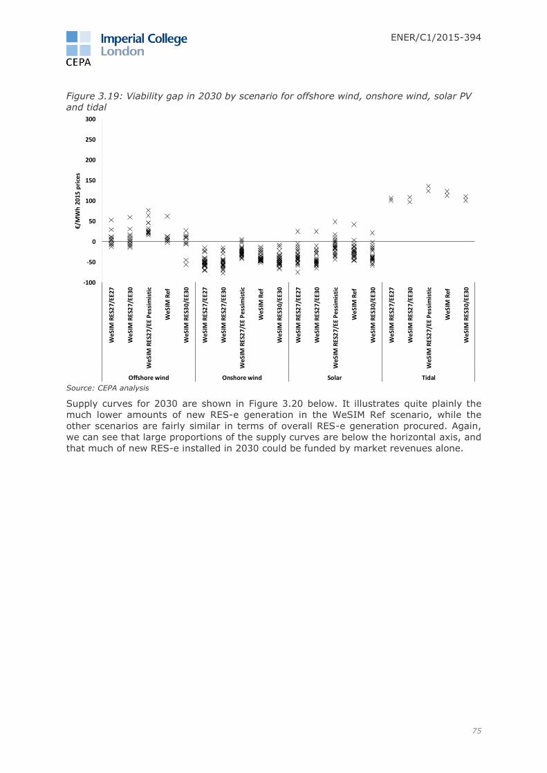
ENER/C1/2015-394

75


and tidal


Supply curves for 2030 are shown in Figure 3.20 below. It illustrates quite plainly the

much lower amounts of new RES-e generation in the WeSIM Ref scenario, while the

other scenarios are fairly similar in terms of overall RES-e generation procured. Again,

we can see that large proportions of the supply curves are below the horizontal axis, and

that much of new RES-e installed in 2030 could be funded by market revenues alone.

-100

-50

0

50

100

150

200

250

300

WeS

IM R

ES2

7/EE

27

We

SIM

RES

27

/EE3

0

We

SIM

RES

27

/EE

Pe

ssim

isti

c

We

SIM

Re

f

We

SIM

RES

30

/EE3

0

We

SIM

RES

27

/EE2

7

We

SIM

RES

27

/EE3

0

We

SIM

RES

27

/EE

Pe

ssim

isti

c

We

SIM

Re

f

We

SIM

RES

30

/EE3

0

WeS

IM R

ES2

7/EE

27

WeS

IM R

ES2

7/EE

30

WeS

IM R

ES2

7/EE

Pes

sim

isti

c

WeS

IM R

ef

WeS

IM R

ES3

0/EE

30

We

SIM

RES

27

/EE2

7

We

SIM

RES

27

/EE3

0

We

SIM

RES

27

/EE

Pe

ssim

isti

c

We

SIM

Re

f

We

SIM

RES

30

/EE3

0


€/M

Wh

20

15

pri

ces

ENER/C1/2015-394

76



Figure 3.20 shows that significant changes in RES-e viability occur between 2020 and

2030:

over the ten-year period, we see a large improvement in viability across the

board; two additional RES-e technologies become fully viable in all locations in

all but one scenario; and

viability gaps primarily remain for offshore wind, biomass, tidal and some less

favourable solar PV locations.

2050 scenarios

Figure 3.21, Figure 3.22 and Figure 3.23 show RES-e viability in 2050. When compared

to the previous figures, one can see the evolution of RES-e viability between 2020 and

2030. In particular, the trend over time is towards increasing viability, with lower

viability gaps, which is consistent with the persistent upwards trend in electricity prices,

shown in Figure 3.13. By 2050, across all scenarios wholesale electricity prices are high

enough to fully fund investments in geothermal and hydro generation technologies

without any additional support.

-150

-100

-50

0

50

100

150

200

0 5 10 15 20 25 30 35 40 45

€/M

Wh

20

15

pri

ces

Production in TWh


ENER/C1/2015-394

77

Figure 3.21: Viability gap in 2050 by scenario for biomass, geothermal, hydro reservoir

and hydro ROR


For wind, solar and tidal technologies the results also show a strong tendency towards

increasing viability by 2050, though in some scenarios there are a few technology and

country pairings that still require additional support (see Figure 3.22). In particular, for

the WeSIM RES27/EE Pessimistic scenario, which has the lowest forecasted average

wholesale price, offshore wind, biomass and tidal range continue still need support in

most countries.

-300

-200

-100

0

100

200

300

WeS

IM R

ES2

7/EE

27

We

SIM

RES

27

/EE3

0

We

SIM

RES

27

/EE

Pe

ssim

isti

c

We

SIM

Re

f

We

SIM

RES

30

/EE3

0

We

SIM

RES

27

/EE2

7

We

SIM

RES

27

/EE3

0

We

SIM

RES

27

/EE

Pe

ssim

isti

c

We

SIM

Re

f

We

SIM

RES

30

/EE3

0

WeS

IM R

ES2

7/EE

27

WeS

IM R

ES2

7/EE

30

WeS

IM R

ES2

7/EE

Pes

sim

isti

c

WeS

IM R

ef

WeS

IM R

ES3

0/EE

30

We

SIM

RES

27

/EE2

7

We

SIM

RES

27

/EE3

0

We

SIM

RES

27

/EE

Pe

ssim

isti

c

We

SIM

Re

f

We

SIM

RES

30

/EE3

0


€/M

Wh

20

15

pri

ces

ENER/C1/2015-394

78


and tidal


The 2050 supply curves below show again that most of the RES-e capacity deployed in

that year is viable without additional support mechanisms. The total amount of capacity

that requires support (i.e., falls in the part of the supply curve above the x-axis), is

relatively small in all scenarios, except the WeSIM RES27/EE Pessimistic scenario. This is

primarily caused by the significant number of non-viable, offshore wind projects. For

example, in the WeSIM RES27/EE27 scenario just over 15 TWh of output per annum

requires support in 2050, almost entirely due to offshore wind not being viable in

Germany.

-200

-150

-100

-50

0

50

100

150

200

250

300

WeS

IM R

ES2

7/EE

27

We

SIM

RES

27

/EE3

0

We

SIM

RES

27

/EE

Pe

ssim

isti

c

We

SIM

Re

f

We

SIM

RES

30

/EE3

0

We

SIM

RES

27

/EE2

7

We

SIM

RES

27

/EE3

0

We

SIM

RES

27

/EE

Pe

ssim

isti

c

We

SIM

Re

f

We

SIM

RES

30

/EE3

0

WeS

IM R

ES2

7/EE

27

WeS

IM R

ES2

7/EE

30

WeS

IM R

ES2

7/EE

Pes

sim

isti

c

WeS

IM R

ef

WeS

IM R

ES3

0/EE

30

We

SIM

RES

27

/EE2

7

We

SIM

RES

27

/EE3

0

We

SIM

RES

27

/EE

Pe

ssim

isti

c

We

SIM

Re

f

We

SIM

RES

30

/EE3

0


€/M

Wh

20

15

pri

ces

ENER/C1/2015-394

79



Between 2030 and 2050 the following trends in RES-e viability are discernible:

there are continued improvements in viability for most RES-e technologies, most

notably for tidal, which significantly closes the gap on offshore wind, though

progress for biomass is limited given its high marginal fuel costs; and

with the increased level of RES-e penetration, differences in scenarios are now

more pronounced than in earlier years. In particular, this is the case in the

WeSIM RES27/EE30 scenario, where we find all RES-e to be fully viable without

support.

2030 sensitivities

In addition to the five main scenarios, we examine how a set of sensitivities on the

WeSIM RES27/EE27 scenario affects the viability gap in 2030. In these cases, certain

market features are flexed, but the overall investment challenge shown above in Figure

3.12 remains unchanged. We present the estimated viability gaps for these sensitivities

in 2030 in Figure 3.24 and Figure 3.25.

-200

-150

-100

-50

0

50

100

0 20 40 60 80 100 120 140 160

€/M

Wh

20

15

pri

ces

Production in TWh


ENER/C1/2015-394

80

Figure 3.24: Viability gap in 2030 by sensitivity for biomass, geothermal, hydro reservoir

and hydro ROR


Figure 3.25: Viability gap in 2030 by sensitivity for offshore wind, onshore wind, solar PV

and tidal


Figure 3.24 and Figure 3.25 highlight important differences between RES-e technologies

under the different sensitivities:

-150

-100

-50

0

50

100

150

200

250

300

We

SIM

RES

27

/EE2

7

Low

er

ETS

No

pre

f ru

les

Low

off

sho

re c

ost

WA

CC

+1

%

WA

CC

+2

%

Imp

erf

ect

fo

resi

ght

Nat

iona

l CR

Ms

WeS

IM R

ES2

7/EE

27

Low

er

ETS

No

pre

f ru

les

Low

off

sho

re c

ost

WA

CC

+1

%

WA

CC

+2

%

Impe

rfec

t fo

resi

ght

Nat

ion

al C

RM

s

We

SIM

RES

27

/EE2

7

Low

er

ETS

No

pre

f ru

les

Low

off

shor

e co

st

WA

CC

+1

%

WA

CC

+2

%

Imp

erf

ect

fo

resi

ght

Nat

ion

al C

RM

s

We

SIM

RES

27

/EE2

7

Low

er

ETS

No

pre

f ru

les

Low

off

sho

re c

ost

WA

CC

+1

%

WA

CC

+2

%

Impe

rfec

t fo

resi

ght

Nat

iona

l CR

Ms


€/M

Wh

20

15

pri

ces

-100

-50

0

50

100

150

200

250

300

We

SIM

RES

27

/EE2

7

Low

er

ETS

No

pre

f ru

les

Low

off

sho

re c

ost

WA

CC

+1

%

WA

CC

+2

%

Imp

erf

ect

fo

resi

ght

Nat

iona

l CR

Ms

WeS

IM R

ES2

7/EE

27

Low

er

ETS

No

pre

f ru

les

Low

off

sho

re c

ost

WA

CC

+1

%

WA

CC

+2

%

Impe

rfec

t fo

resi

ght

Nat

ion

al C

RM

s

We

SIM

RES

27

/EE2

7

Low

er

ETS

No

pre

f ru

les

Low

off

shor

e co

st

WA

CC

+1

%

WA

CC

+2

%

Imp

erf

ect

fo

resi

ght

Nat

ion

al C

RM

s

We

SIM

RES

27

/EE2

7

Low

er

ETS

No

pre

f ru

les

Low

off

sho

re c

ost

WA

CC

+1

%

WA

CC

+2

%

Impe

rfec

t fo

resi

ght

Nat

iona

l CR

Ms


€/M

Wh

20

15

pri

ces

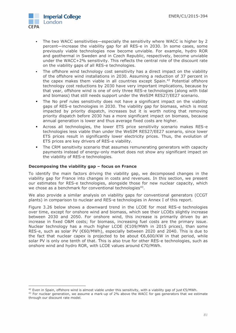
ENER/C1/2015-394

81

The two WACC sensitivities—especially the sensitivity where WACC is higher by 2

percent—increase the viability gap for all RES-e in 2030. In some cases, some

previously viable technologies now become unviable. For example, hydro ROR

and geothermal in Sweden and in Czech Republic, respectively, become unviable

under the WACC+2% sensitivity. This reflects the central role of the discount rate

on the viability gaps of all RES-e technologies.

The offshore wind technology cost sensitivity has a direct impact on the viability

of the offshore wind installations in 2030. Assuming a reduction of 37 percent in

the capex makes them viable in all countries except Spain.42 Potential offshore

technology cost reductions by 2030 have very important implications, because by

that year, offshore wind is one of only three RES-e technologies (along with tidal

and biomass) that still needs support under the WeSIM RES27/EE27 scenario.

The No pref rules sensitivity does not have a significant impact on the viability

gaps of RES-e technologies in 2030. The viability gap for biomass, which is most

impacted by priority dispatch, increases but it is worth noting that removing

priority dispatch before 2030 has a more significant impact on biomass, because

annual generation is lower and thus average fixed costs are higher.

Across all technologies, the lower ETS price sensitivity scenario makes RES-e

technologies less viable than under the WeSIM RES27/EE27 scenario, since lower

ETS prices result in significantly lower electricity prices. Thus, the evolution of

ETS prices are key drivers of RES-e viability.

The CRM sensitivity scenario that assumes remunerating generators with capacity

payments instead of energy-only market does not show any significant impact on

the viability of RES-e technologies.

Decomposing the viability gap – focus on France

To identify the main factors driving the viability gap, we decomposed changes in the

viability gap for France into changes in costs and revenues. In this section, we present

our estimates for RES-e technologies, alongside those for new nuclear capacity, which

we chose as a benchmark for conventional technologies43.

We also provide a similar analysis on viability gaps for conventional generators (CCGT

plants) in comparison to nuclear and RES-e technologies in Annex I of this report.

Figure 3.26 below shows a downward trend in the LCOE for most RES-e technologies

over time, except for onshore wind and biomass, which see their LCOEs slightly increase

between 2030 and 2050. For onshore wind, this increase is primarily driven by an

increase in fixed O&M costs; for biomass, increasing fuel costs are the primary issue.

Nuclear technology has a much higher LCOE (€109/MWh in 2015 prices), than some

RES-e, such as solar PV (€60/MWh), especially between 2020 and 2040. This is due to

the fact that nuclear capex is projected to be about €6,600/KW in that period, while

solar PV is only one tenth of that. This is also true for other RES-e technologies, such as

onshore wind and hydro ROR, with LCOE values around €70/MWh.

42 Even in Spain, offshore wind is almost viable under this sensitivity, with a viability gap of just €5/MWh. 43 For nuclear generation, we assume a mark-up of 2% above the WACC for gas generators that we estimate through our discount rate model.

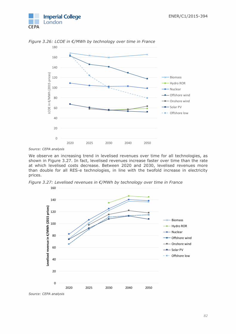
ENER/C1/2015-394

82

Figure 3.26: LCOE in €/MWh by technology over time in France


We observe an increasing trend in levelised revenues over time for all technologies, as

shown in Figure 3.27. In fact, levelised revenues increase faster over time than the rate

at which levelised costs decrease. Between 2020 and 2030, levelised revenues more

than double for all RES-e technologies, in line with the twofold increase in electricity

prices.

Figure 3.27: Levelised revenues in €/MWh by technology over time in France


0

20

40

60

80

100

120

140

160

180

2020 2025 2030 2040 2050

LCO

E in

€/M

Wh

(201

5 p

rice

s)

Biomass

Hydro ROR

Nuclear

Offshore wind

Onshore wind

Solar PV

Offshore low

0

20

40

60

80

100

120

140

160

2020 2025 2030 2040 2050

Leve

lise

d r

eve

nu

e in

€/M

Wh

(2

01

5 p

rice

s)

Biomass

Hydro ROR

Nuclear

Offshore wind

Onshore wind

Solar PV

Offshore low

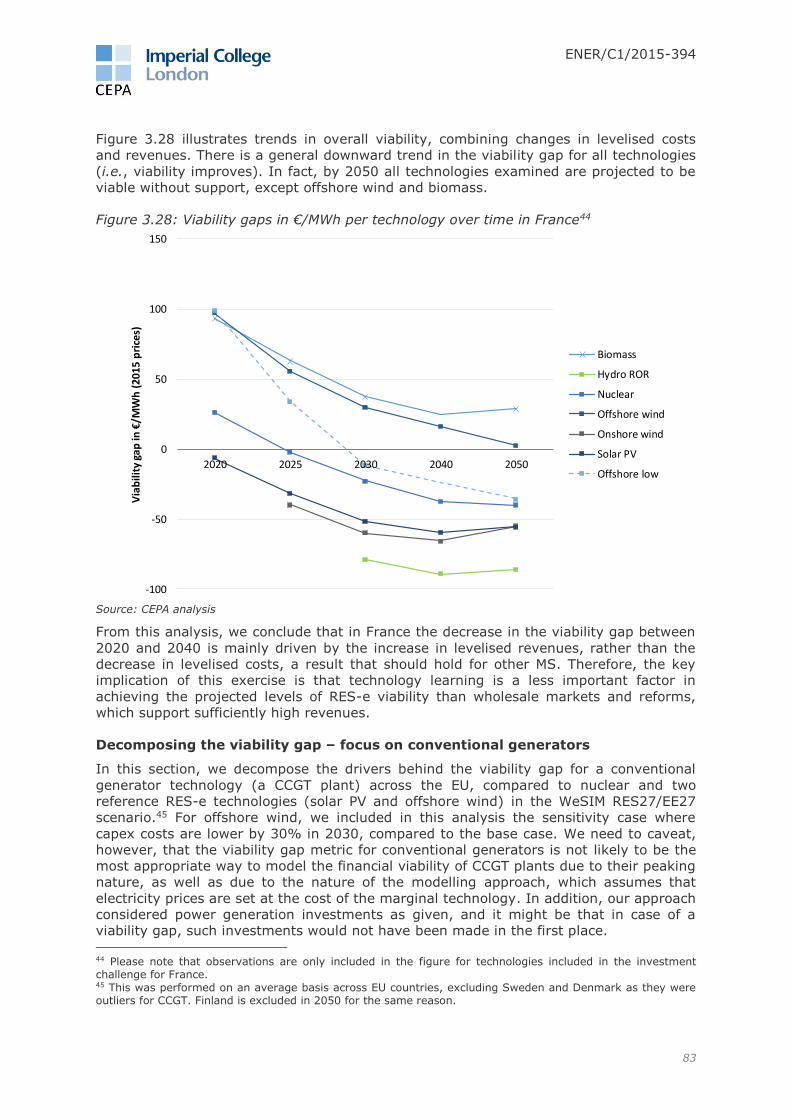
ENER/C1/2015-394

83

Figure 3.28 illustrates trends in overall viability, combining changes in levelised costs

and revenues. There is a general downward trend in the viability gap for all technologies

(i.e., viability improves). In fact, by 2050 all technologies examined are projected to be

viable without support, except offshore wind and biomass.

Figure 3.28: Viability gaps in €/MWh per technology over time in France44


From this analysis, we conclude that in France the decrease in the viability gap between

2020 and 2040 is mainly driven by the increase in levelised revenues, rather than the

decrease in levelised costs, a result that should hold for other MS. Therefore, the key

implication of this exercise is that technology learning is a less important factor in

achieving the projected levels of RES-e viability than wholesale markets and reforms,

which support sufficiently high revenues.

Decomposing the viability gap – focus on conventional generators

In this section, we decompose the drivers behind the viability gap for a conventional

generator technology (a CCGT plant) across the EU, compared to nuclear and two

reference RES-e technologies (solar PV and offshore wind) in the WeSIM RES27/EE27

scenario.45 For offshore wind, we included in this analysis the sensitivity case where

capex costs are lower by 30% in 2030, compared to the base case. We need to caveat,

however, that the viability gap metric for conventional generators is not likely to be the

most appropriate way to model the financial viability of CCGT plants due to their peaking

nature, as well as due to the nature of the modelling approach, which assumes that

electricity prices are set at the cost of the marginal technology. In addition, our approach

considered power generation investments as given, and it might be that in case of a

viability gap, such investments would not have been made in the first place.

44 Please note that observations are only included in the figure for technologies included in the investment challenge for France. 45 This was performed on an average basis across EU countries, excluding Sweden and Denmark as they were outliers for CCGT. Finland is excluded in 2050 for the same reason.

-100

-50

0

50

100

150

2020 2025 2030 2040 2050

Via

bili

ty g

ap in

€/M

Wh

(20

15 p

rice

s)

Biomass

Hydro ROR

Nuclear

Offshore wind

Onshore wind

Solar PV

Offshore low

ENER/C1/2015-394

84

Figure 3.29 compares LCOE for CCGTs to the LCOE of nuclear and RES-e technologies.

Our first observation is that CCGT has the highest LCOE, over €200/MWh, between 2020

and 2025. In contrast, nuclear and the reference RES-e technologies have LCOEs closer

to €100/MWh. This is explained by the fact that between 2020 and 2030 CCGTs are

projected to generate relatively little in the WeSIM RES27/EE27 scenario, which pushes

up their LCOE.

A second observation is that contrary to nuclear and RES-e technologies, the LCOE for

CCGTs sharply increases between 2040 and 2050, directly driven by the increase in

carbon prices, which double in that period.

Figure 3.29: LCOE in €/MWh by technology over time in EU28 under WeSIM RES27/EE27

scenario


Figure 3.30 below compares the levelised revenue for CCGTs under the WeSIM

RES27/EE27 scenario to nuclear and RES-e technologies. Clearly, there is a large

increase in levelised CCGT revenues between 2040 and 2050, in contrast to the other

technologies. The main reason for this is that CCGTs only generate when electricity

prices are high, usually during peak periods, reflecting the fact that they tend to be at

the end of the merit order. This weighted average price received by CCGT generators is

projected to triple between 2040 and 2050, reaching €730/MWh, compared to

€134/MWh for nuclear and €105/MWh for solar PV.

0

200

400

600

800

1,000

1,200

1,400

2020 2025 2030 2040 2050

Ave

rage

LC

OE

in €

/MW

h (

20

15

pri

ces)

CCGT

Nuclear

Offshore wind

Solar PV

Offshore low

ENER/C1/2015-394

85

Figure 3.30: Levelised revenue in €/MWh by technology over time in EU28 under WeSIM

RES27/EE27 scenario


Figure 3.31 below highlights the difference in the viability gap between CCGTs, nuclear

and RES-e technologies. Similarly to nuclear and the RES-e technologies, the CCGT

viability gap follows a downward trend until 2025, but it sharply increases thereafter,

reaching a high of €700/MWh by 2050. This upward trend in CCGT’s viability gap is the

result of the increase in LCOE. The increase in LCOE more than offsets the increase in

levelised revenues for CCGT, thus resulting in a growing viability gap.

0

100

200

300

400

500

600

700

800

2020 2025 2030 2040 2050

Ave

rage

Lev

elis

ed R

even

ue

in €

/MW

h (

20

15

pri

ces)

CCGT

Nuclear

Offshore wind

Solar PV

Offshore low

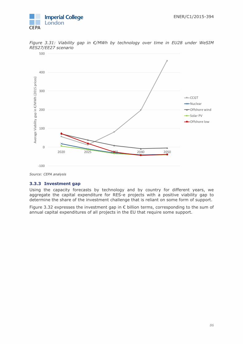
ENER/C1/2015-394

86

Figure 3.31: Viability gap in €/MWh by technology over time in EU28 under WeSIM

RES27/EE27 scenario


3.3.3 Investment gap

Using the capacity forecasts by technology and by country for different years, we

aggregate the capital expenditure for RES-e projects with a positive viability gap to

determine the share of the investment challenge that is reliant on some form of support.

Figure 3.32 expresses the investment gap in € billion terms, corresponding to the sum of

annual capital expenditures of all projects in the EU that require some support.

-100

0

100

200

300

400

500

2020 2025 2030 2040 2050

Ave

rage

Via

bili

ty g

ap in

€/M

Wh

(2

01

5 p

rice

s)

CCGT

Nuclear

Offshore wind

Solar PV

Offshore low

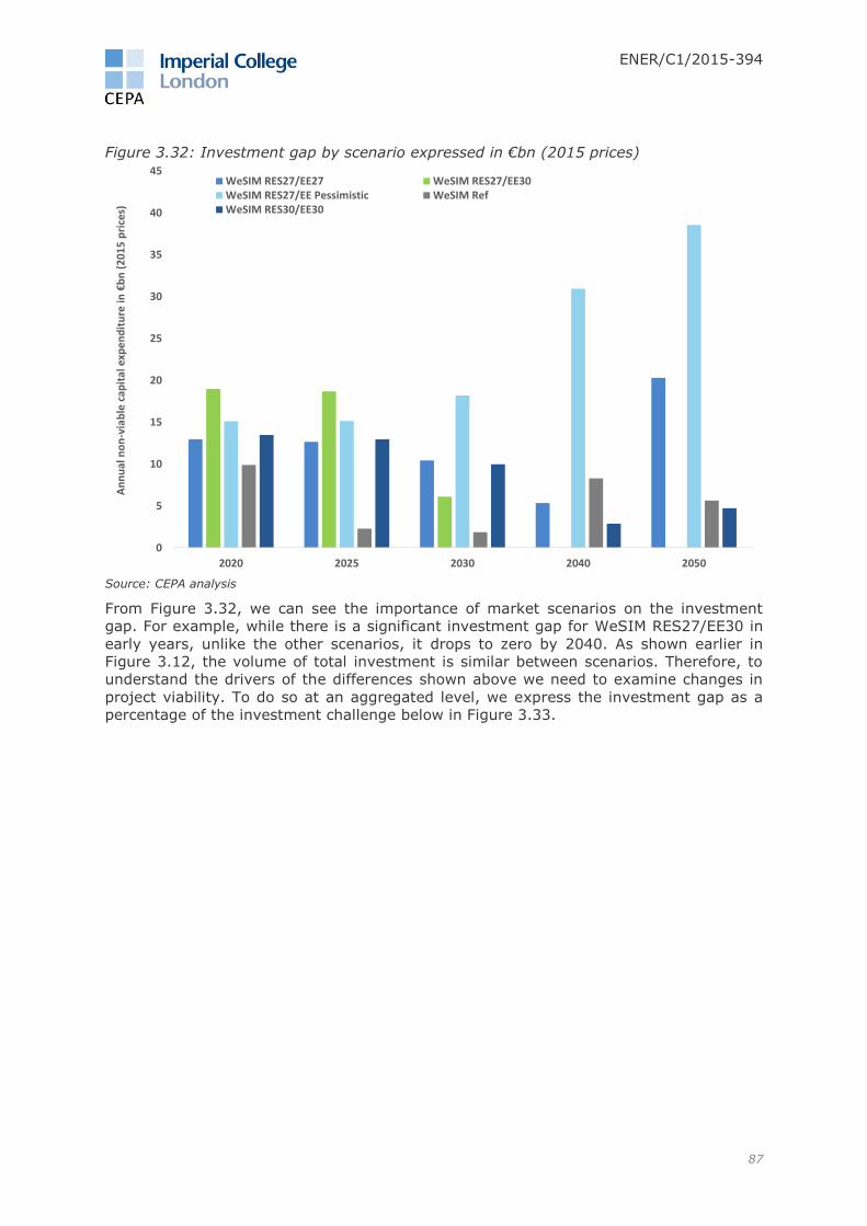
ENER/C1/2015-394

87

Figure 3.32: Investment gap by scenario expressed in €bn (2015 prices)


From Figure 3.32, we can see the importance of market scenarios on the investment

gap. For example, while there is a significant investment gap for WeSIM RES27/EE30 in

early years, unlike the other scenarios, it drops to zero by 2040. As shown earlier in

Figure 3.12, the volume of total investment is similar between scenarios. Therefore, to

understand the drivers of the differences shown above we need to examine changes in

project viability. To do so at an aggregated level, we express the investment gap as a

percentage of the investment challenge below in Figure 3.33.

0

5

10

15

20

25

30

35

40

45

2020 2025 2030 2040 2050

An

nu

al n

on

-via

ble

cap

ital

exp

en

dit

ure

in €

bn

(2

01

5 p

rice

s)

WeSIM RES27/EE27 WeSIM RES27/EE30WeSIM RES27/EE Pessimistic WeSIM RefWeSIM RES30/EE30

ENER/C1/2015-394

88


scenario


Figure 3.33 shows that across all scenarios, around half of the required RES-e

investments in 2020 are not viable based on wholesale market revenues alone, and

therefore require public support. This share decreases rapidly for the WeSIM

RES27/EE27 and WeSIM RES27/EE30 scenarios and the WeSIM Ref scenario, in

particular between 2025 and 2030. Under the WeSIM RES27/EE30 scenario, we see that

no further support is required for investment in new RES-e projects by 2040. This has a

profound impact on our investment gap estimates, for example compared to the WeSIM

RES27/EE Pessimistic scenario where many projects do not become viable until much

later, as it is in the later years that the largest volume of projects needs to be delivered.

The WeSIM Ref scenario shows a relatively low share of projects that are not viable in

2025 and 2030, compared to other scenarios. This can be explained by the projected

RES-e deployment in that scenario, which includes less RES-e penetration, and therefore

a weaker cannibalisation effect, making the individual projects more viable. Also

electricity demand in those two years is higher than in the WeSIM RES27/EE27 and

WeSIM RES27/EE30 scenarios, thus yielding higher electricity prices and revenues.

We follow the same analysis for the sensitivities around the WeSIM RES27/EE27

scenario. As the investment challenge is the same for all the sensitivities, we focus on

the share of capex, which is not viable compared to the investment challenge, rather

than the absolute value of the investment gap.

Figure 3.34 below shows the share of the investment challenge, for all RES-e in the EU,

which will require some public support.

0%

10%

20%

30%

40%

50%

60%

70%

80%

90%

100%

WeS

IM R

ES2

7/E

E27

WeS

IM R

ES2

7/E

E30

WeS

IM R

ES27

/EE2

7 Pe

ssim

isti

c

WeS

IM R

ef

WeS

IM R

ES3

0/E

E30

WeS

IM R

ES2

7/E

E27

WeS

IM R

ES2

7/E

E30

WeS

IM R

ES27

/EE2

7 Pe

ssim

isti

c

WeS

IM R

ef

WeS

IM R

ES3

0/E

E30

WeS

IM R

ES2

7/E

E27

WeS

IM R

ES2

7/E

E30

WeS

IM R

ES27

/EE2

7 Pe

ssim

isti

c

WeS

IM R

ef

WeS

IM R

ES3

0/E

E30

WeS

IM R

ES2

7/E

E27

WeS

IM R

ES2

7/E

E30

WeS

IM R

ES27

/EE2

7 Pe

ssim

isti

c

WeS

IM R

ef

WeS

IM R

ES3

0/E

E30

WeS

IM R

ES2

7/E

E27

WeS

IM R

ES2

7/E

E30

WeS

IM R

ES27

/EE2

7 Pe

ssim

isti

c

WeS

IM R

ef

WeS

IM R

ES3

0/E

E30

2020 2025 2030 2040 2050

Totalcapex

Non-viablecapex

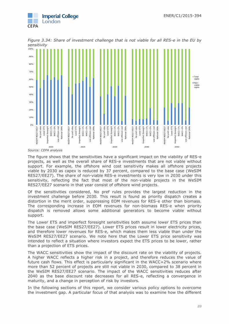
ENER/C1/2015-394

89


sensitivity


The figure shows that the sensitivities have a significant impact on the viability of RES-e

projects, as well as the overall share of RES-e investments that are not viable without

support. For example, the offshore wind cost sensitivity makes all offshore projects

viable by 2030 as capex is reduced by 37 percent, compared to the base case (WeSIM

RES27/EE27). The share of non-viable RES-e investments is very low in 2030 under this

sensitivity, reflecting the fact that most of the non-viable projects in the WeSIM

RES27/EE27 scenario in that year consist of offshore wind projects.

Of the sensitivities considered, No pref rules provides the largest reduction in the

investment challenge before 2030. This result is found as priority dispatch creates a

distortion in the merit order, suppressing EOM revenues for RES-e other than biomass.

The corresponding increase in EOM revenues for non-biomass RES-e when priority

dispatch is removed allows some additional generators to become viable without

support.

The Lower ETS and imperfect foresight sensitivities both assume lower ETS prices than

the base case (WeSIM RES27/EE27). Lower ETS prices result in lower electricity prices,

and therefore lower revenues for RES-e, which makes them less viable than under the

WeSIM RES27/EE27 scenario. We note here that the Lower ETS price sensitivity was

intended to reflect a situation where investors expect the ETS prices to be lower, rather

than a projection of ETS prices.

The WACC sensitivities show the impact of the discount rate on the viability of projects.

A higher WACC reflects a higher risk in a project, and therefore reduces the value of

future cash flows. This effect is particularly significant in the WACC+2% scenario where

more than 52 percent of projects are still not viable in 2030, compared to 38 percent in

the WeSIM RES27/EE27 scenario. The impact of the WACC sensitivities reduces after

2040 as the base discount rate decreases for all RES-e, reflecting a convergence in

maturity, and a change in perception of risk by investors.

In the following sections of this report, we consider various policy options to overcome

the investment gap. A particular focus of that analysis was to examine how the different

0%

10%

20%

30%

40%

50%

60%

70%

80%

90%

100%

WeSIM

RES27/E

E27

No p

ref

rule

s

Low

er

ETS

Imperf

ect

fore

sig

ht

WACC+

1%

WACC+

2%

Low

offshore

cost

National CRM

s

WeSIM

RES27/E

E27

No p

ref

rule

s

Low

er

ETS

Imperf

ect

fore

sig

ht

WACC+

1%

WACC+

2%

Low

offshore

cost

National CRM

s

WeSIM

RES27/E

E27

No p

ref

rule

s

Low

er

ETS

Imperf

ect

fore

sig

ht

WACC+

1%

WACC+

2%

Low

offshore

cost

National CRM

s

WeSIM

RES27/E

E27

No p

ref

rule

s

Low

er

ETS

Imperf

ect

fore

sig

ht

WACC+

1%

WACC+

2%

Low

offshore

cost

National CRM

s

WeSIM

RES27/E

E27

No p

ref

rule

s

Low

er

ETS

Imperf

ect

fore

sig

ht

WACC+

1%

WACC+

2%

Low

offshore

cost

National CRM

s

2020 2025 2030 2040 2050

Totalcapex

Non-viablecapex

ENER/C1/2015-394

90

support options change the risk profile of RES-e investments, and thus potentially reduce

the cost of support.

ENER/C1/2015-394

91

4 Policy options to address the RES-e investment challenge

This section summarises our approach to identifying policy options for RES-e support.

This is followed by a summary of the feedback we received from participants of the June

2016 workshop held in Brussels. At the end of this section, we discuss issues related to

the key design elements of the considered support options. A detailed description of the

policy options considered in this study is contained in Annex D.

4.1 Approach to identifying policy options

The RES-e supply curves presented in Section 3.3 are a function of the assumed cost of

capital, which in turn depends on the underlying risks involved in each policy option.

There is a range of policy options that can potentially reduce the cost of capital, and thus

shift the RES-e supply curves to right, reducing the overall investment challenge.

However, these options involve trade-offs. While providing more certainty to investors

reduces the cost of capital, doing so also shifts some risks and costs to the consumers.

We considered these trade-offs in the process of identifying and assessing the various

policy options.

To identify the detailed policy option designs, we applied the guiding principles listed in

Section 2.3. The implications of these guiding principles on option design are as follows:

options should make investors reasonably confident that the level of support will

fill in their financing gap;

individual MS, regional groupings or the EU are able to make a commitment, and

receive public support, to provide the necessary financial support for the least-

cost mixed of RES-e technologies to meet the RES-e target (i.e., support will not

be reduced at any point due to a lack of funds);

technology neutrality should be implemented in the primary support mechanism

(i.e., all technologies get the same support per MWh);

rely on competitive allocation processes whenever feasible (uniform price

auctions; limited administrative schemes);

we assume that the provisions of State Aid Guidelines will apply beyond 2020

(e.g., no support for food-based biofuel);

the preferred option should be relatively simple and implementable, although

there may be some trade-offs between this and other objectives; and

eligibility is restricted to RES-e technologies that are projected to have a viability

gap.

Taking these principles and implications into account, we applied a best-practices

approach to selecting individual options designs and specific design elements. This

assessment took into account designs and features that have worked well in practice, as

well as those that did not. We have assumed design features that may not have been

implemented in practice, if there was a good reason to do so; for example, if particular

features are likely to achieve a better alignment with our guiding principles than designs,

which have already been implemented in practice. As a result, the designs we analyse

may not reflect precisely any particular support scheme that has already been

implemented in practice.

4.2 Policy option designs chosen for detailed analysis

In this section, we discuss specific policy option designs, summarised in Figure 4.1,

analysed in detail in this study. These options span the range of potential support

mechanisms to include operating and investment aid, market rules and targeted

approaches to address specific market failures.

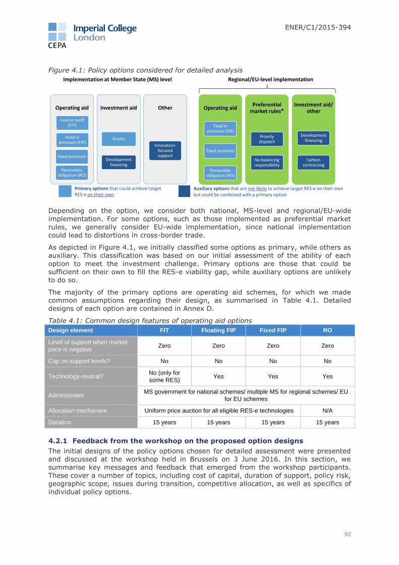
ENER/C1/2015-394

92

Figure 4.1: Policy options considered for detailed analysis

Depending on the option, we consider both national, MS-level and regional/EU-wide

implementation. For some options, such as those implemented as preferential market

rules, we generally consider EU-wide implementation, since national implementation

could lead to distortions in cross-border trade.

As depicted in Figure 4.1, we initially classified some options as primary, while others as

auxiliary. This classification was based on our initial assessment of the ability of each

option to meet the investment challenge. Primary options are those that could be

sufficient on their own to fill the RES-e viability gap, while auxiliary options are unlikely

to do so.

The majority of the primary options are operating aid schemes, for which we made

common assumptions regarding their design, as summarised in Table 4.1. Detailed

designs of each option are contained in Annex D.

Table 4.1: Common design features of operating aid options

Design element FIT Floating FIP Fixed FIP RO

Level of support when market

price is negative Zero Zero Zero Zero

Cap on support levels? No No No No

Technology-neutral? No (only for

some RES) Yes Yes Yes

Administrator MS government for national schemes/ multiple MS for regional schemes/ EU

for EU schemes

Allocation mechanism Uniform price auction for all eligible RES-e technologies N/A

Duration 15 years 15 years 15 years 15 years

4.2.1 Feedback from the workshop on the proposed option designs

The initial designs of the policy options chosen for detailed assessment were presented

and discussed at the workshop held in Brussels on 3 June 2016. In this section, we

summarise key messages and feedback that emerged from the workshop participants.

These cover a number of topics, including cost of capital, duration of support, policy risk,

geographic scope, issues during transition, competitive allocation, as well as specifics of

individual policy options.

Operating aid

Feed in tariff (FIT)

Feed in premium (FIP)

Fixed premium

Renewable obligation (RO)

Investment aid

Grants

Development financing

Other

Innovation-focused support

Operating aid

Feed in premium (FIP)

Fixed premium

Renewable obligation (RO)

Preferential market rules*

Priority dispatch

No balancing responsibility

Investment aid/ other


Carbon contracting

Implementation at Member State (MS) level Regional/EU-level implementation

Primary options that could achieve target RES-e on their own

Auxiliary options that are not likely to achieve target RES-e on their own but could be combined with a primary option

ENER/C1/2015-394

93

Cost of capital estimates

CEPA presented its initial cost of capital estimates by policy option and by RES-e

technology for 2020 and 2030. These estimates were generally seen as appropriate.

Concerning the cost of capital, the following two specific suggestion were made:

biomass should be treated as separate asset class to reflect higher operational

risk, and therefore have a higher cost of capital; and

the estimated spread between hydro ROR and hydro reservoir technologies was

seen to be too wide.

In response to this feedback, we adjusted our cost of capital estimates as follows:

in order to more accurately reflect the higher operational and construction risks

for biomass, we increased its cost of capital, so that the spread between biomass

and solar PV was increased to two percentage points;

we adjusted the cost of capital for hydro reservoir to obtain a spread of 0.7

percentage points between the hydro reservoir and hydro ROR technologies; and

to reflect geological risks associated with geothermal generators, we increased

the spread between geothermal and solar PV to 6 percentage points.

Duration of support

There was a strong reaction to our initial assumption of a 10-year subsidy life.

Participants have expressed concerns that, with the duration of RES-e support being a

crucial parameter for RES-e investors, 10 years may be too short. A relatively short

subsidy life could mean that debt investors would seek returns earlier, deferring returns

to equity holders, and thus potentially increasing the cost of equity and the overall cost

of capital.

Workshop participants also stated that the duration of RES-e support is especially

important for RES-e technologies that face a higher operational, fuel cost and foreign

exchange risks, such as biomass.

Using the feedback from the workshop, we increased our assumption on the duration of

support from 10 years to 15 years for all policy options in the final quantitative analysis.

Policy risk

Policy risk was confirmed by the workshop participants to be the main source of risk in

regard to RES-e support. Workshop participants agreed that some of this risk could be

mitigated through contractual arrangements, but they also pointed out that public

acceptance of RES-e in general, and the willingness to bear the cost of increasing RES-e

generation should also be considered as part of the policy risk.

EU-wide and regional implementation

While they appreciated the potential benefits of RES-e support schemes implemented on

an EU-wide or regional basis, workshop participants do not consider it politically feasible

in the near- to mid-term (i.e., before 2030).

Competitive allocation mechanisms

Some workshop participants were concerned about the impact of competitive allocation

mechanisms on innovation given it may not be possible to recoup innovation-related

expenses within a single tender round. They argued this could be an issue for investors

in innovation if others can free-ride on their learning in future rounds, and therefore

questioned the appropriateness of such mechanisms for emerging technologies in

particular.

ENER/C1/2015-394

94

On the other hand, it was noted that a technology-neutral approach would unlock

opportunities for lower-cost RES-e technologies. Some participants also noted that under

technology-specific allocation mechanisms, investors might be discouraged from other

innovative but non-renewable investments that could help support the achievement of

decarbonisation objectives, such as those to unlock demand side response or storage

technologies.

Transition towards viability

It was argued that investors may find it difficult to transition away from RES-e subsidies;

therefore such transition should be carefully managed.

Development finance

Workshop participants noted that existing development (subsidised) finance from

institutions such as the European Investment Bank (EIB) and the UK Green Investment

Bank, are very important as they provide sufficient funding for RES-e, as well as liquidity

for emerging technologies that are close to being bankable.

Development finance also works well for novel technologies, as well as for large projects.

In that sense, development finance could be considered similar to the “innovation-

focused” support option. Lastly, development finance could also improve the bankability

of RES-e projects if it is based on first loss support.

In response to this feedback, we amended our viability modelling to limit the application

of development finance to technologies that are not yet fully mature, as well as to

offshore wind, due to the size of those projects.


Market participants do not view imbalance costs or priority dispatch as crucial factors for

RES-e investment. They expressed concern about preferential market rules—such as

exemptions from balancing responsibility or priority dispatch—because they could

negatively impact the wholesale electricity market as a whole.

Although preferential market rules do not appear to be suitable as a primary means of

supporting RES-e, we considered them as measures that could address some market

failures.

Carbon contracting

Carbon contracting was recognised as a targeted measure to mitigate policy risk,

specifically risk associated with ETS prices. However, it was seen as too complex and

unlikely to work in practice. A better option would be to reform the EU ETS, so as to

enhance the credibility of the EU carbon pricing policy.

4.2.2 Discussion of key design elements

In this section, we discuss in further detail some of the design elements, including those

that received the most feedback from workshop participants.

Technology neutrality

The main reason for technology neutrality is to allow different RES-e to compete side-by-

side for support in a competitive allocation mechanism. This approach is most likely to

minimise the overall cost of RES-e support because they:

minimise the reliance on administrative parameters (e.g., setting different levels

of support for different types of RES-e), which often turn out to be erroneous and

result in overcompensation;

ENER/C1/2015-394

95

deliver the least-cost mix of RES-e required to meet the target, as long as the

allocation mechanism is competitive; and

some workshop participants have challenged the principle of technology

neutrality, arguing that it could fail to fully account for carbon reductions outside

the electricity sector (e.g., renewable heat, CHP), and that it may not achieve a

desired level of resource diversity.

We note that our modelling relies on PRIMES scenarios, where carbon abatement is

considered (by PRIMES) across all energy uses, not just in the electricity sector. Thus,

the RES-e capacity projections we used are part of the least-cost mix of measures to

achieve the decarbonisation targets. More importantly, we consider that the asymmetric

information problem regarding technology costs between investors and governments will

likely remain. The best way to address it is to award RES-e support in competitive,

technology-neutral mechanisms—truly competitive auctions should provide adequate

incentive to RES-e investors to reflect their true technology costs in their bids. These

bids would also reflect their own best estimate of other costs and revenues going

forward. Many of these costs are specific to the individual projects, and thus it would be

difficult for anyone, but the developer, to accurately estimate them.

Regarding resource diversity, we note that the PRIMES RES-e projections already exhibit

a fair amount of diversity in terms of technology type, hourly generation profile and

location. Further resource diversity could be achieved by an auxiliary, innovation-focused

support mechanism, but there are no compelling reasons to make the primary support

mechanism not a technology-neutral one.

Duration of support

Applying a uniform duration for the support schemes is necessary in order to implement

technology neutrality, especially since the objective is to support RES-e by means of a

relatively simple and transparent mechanism. This implies that some RES-e technologies

would not receive support for their entire economic lives, unless they are allowed to re-

apply for support following the expiration of their initial contract. In our estimates of the

viability gap, we conservatively assumed the position of no support being made available

beyond the initial duration.

Workshop participants indicated that our initial assumption of a ten-year support

duration might be too short. After the workshop, we revised our assumed duration to 15

years. We note, however, that there are some trade-offs between the duration of

support and the potential cost to consumers. In terms of market integration, shorter

durations expose generators to market signals for longer periods, but with a higher

initial level of support required, any short-term distortion created has potential to be

more intense. In terms of discount rates, longer durations may provide benefits such as

an extended period of wholesale market risk protection but that may be counterbalanced

by having to wait longer to realise the full value of the support scheme. The balance

between these considerations may vary based upon how far technologies are from

achieving viability without support.

We do not make any specific recommendations regarding subsidy life in this study.

Although the assumed length of subsidy life may affect our quantitative analyses, the

primary RES-e support mechanism we recommend in this study is not affected by this

assumption.

Eligibility

While we uphold the principle that viable RES-e technologies should not receive support,

we note that the specifics of eligibility rules are important. If eligibility rules are not well

designed, it could give rise to perverse incentives. For example, viability metrics used to

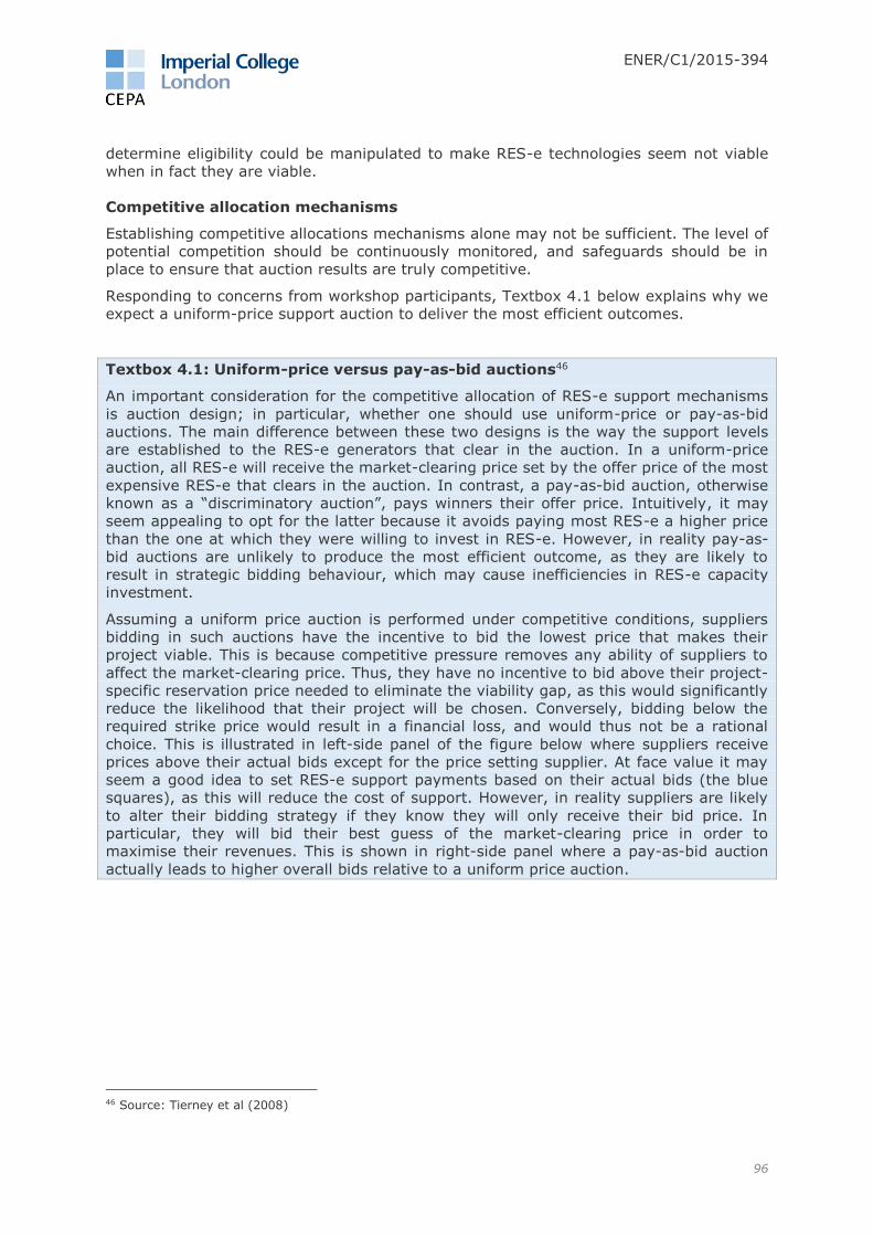
ENER/C1/2015-394

96

determine eligibility could be manipulated to make RES-e technologies seem not viable

when in fact they are viable.

Competitive allocation mechanisms

Establishing competitive allocations mechanisms alone may not be sufficient. The level of

potential competition should be continuously monitored, and safeguards should be in

place to ensure that auction results are truly competitive.

Responding to concerns from workshop participants, Textbox 4.1 below explains why we

expect a uniform-price support auction to deliver the most efficient outcomes.

Textbox 4.1: Uniform-price versus pay-as-bid auctions46

An important consideration for the competitive allocation of RES-e support mechanisms

is auction design; in particular, whether one should use uniform-price or pay-as-bid

auctions. The main difference between these two designs is the way the support levels

are established to the RES-e generators that clear in the auction. In a uniform-price

auction, all RES-e will receive the market-clearing price set by the offer price of the most

expensive RES-e that clears in the auction. In contrast, a pay-as-bid auction, otherwise

known as a “discriminatory auction”, pays winners their offer price. Intuitively, it may

seem appealing to opt for the latter because it avoids paying most RES-e a higher price

than the one at which they were willing to invest in RES-e. However, in reality pay-as-

bid auctions are unlikely to produce the most efficient outcome, as they are likely to

result in strategic bidding behaviour, which may cause inefficiencies in RES-e capacity

investment.

Assuming a uniform price auction is performed under competitive conditions, suppliers

bidding in such auctions have the incentive to bid the lowest price that makes their

project viable. This is because competitive pressure removes any ability of suppliers to

affect the market-clearing price. Thus, they have no incentive to bid above their project-

specific reservation price needed to eliminate the viability gap, as this would significantly

reduce the likelihood that their project will be chosen. Conversely, bidding below the

required strike price would result in a financial loss, and would thus not be a rational

choice. This is illustrated in left-side panel of the figure below where suppliers receive

prices above their actual bids except for the price setting supplier. At face value it may

seem a good idea to set RES-e support payments based on their actual bids (the blue

squares), as this will reduce the cost of support. However, in reality suppliers are likely

to alter their bidding strategy if they know they will only receive their bid price. In

particular, they will bid their best guess of the market-clearing price in order to

maximise their revenues. This is shown in right-side panel where a pay-as-bid auction

actually leads to higher overall bids relative to a uniform price auction.

46 Source: Tierney et al (2008)

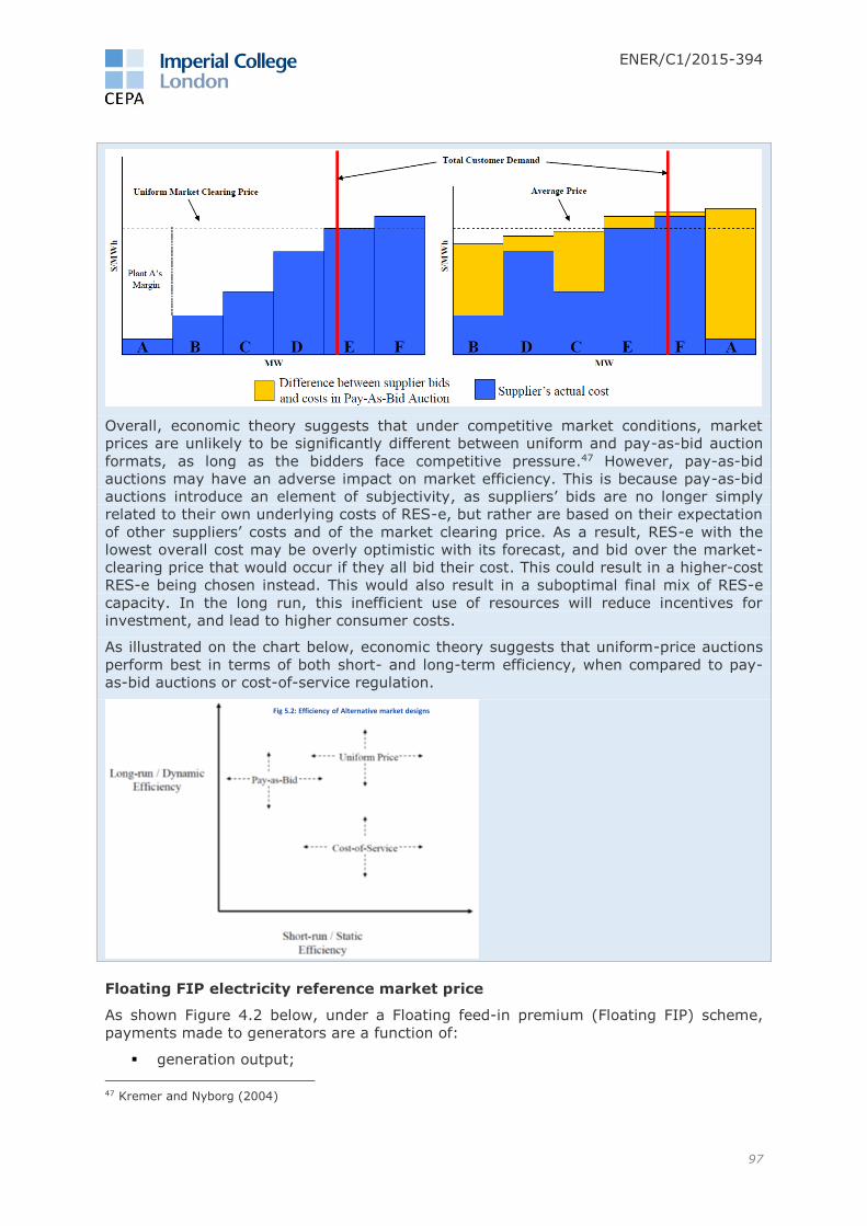
ENER/C1/2015-394

97

Overall, economic theory suggests that under competitive market conditions, market

prices are unlikely to be significantly different between uniform and pay-as-bid auction

formats, as long as the bidders face competitive pressure.47 However, pay-as-bid

auctions may have an adverse impact on market efficiency. This is because pay-as-bid

auctions introduce an element of subjectivity, as suppliers’ bids are no longer simply

related to their own underlying costs of RES-e, but rather are based on their expectation

of other suppliers’ costs and of the market clearing price. As a result, RES-e with the

lowest overall cost may be overly optimistic with its forecast, and bid over the market-

clearing price that would occur if they all bid their cost. This could result in a higher-cost

RES-e being chosen instead. This would also result in a suboptimal final mix of RES-e

capacity. In the long run, this inefficient use of resources will reduce incentives for

investment, and lead to higher consumer costs.

As illustrated on the chart below, economic theory suggests that uniform-price auctions

perform best in terms of both short- and long-term efficiency, when compared to pay-

as-bid auctions or cost-of-service regulation.

Floating FIP electricity reference market price

As shown Figure 4.2 below, under a Floating feed-in premium (Floating FIP) scheme,

payments made to generators are a function of:

generation output;

47 Kremer and Nyborg (2004)

Fig 5.1A: Uniform price auction Fig 5.1B: Pay-as-Bid auction

Fig 5.2: Efficiency of Alternative market designs

ENER/C1/2015-394

98

a strike price;48 and

a market reference price.49

Figure 4.2: Characterisation of a Floating FIP

Source: UK DECC 2011 White Paper, p38 available here

In this section, we consider the impact of choosing reference market prices (RMP) set

over different timescales on the incentives of generators to respond to wholesale market

prices. We examine how different options affect “basis risk,” which arises when the RMP

diverges from the price realised by a generator.50 Lastly, we present out findings of the

potential relative magnitude of impacts on different types of generators using revenues

calculated using WeSIM under the WeSIM RES27/EE27 scenario in 2030. We address

each area in turn.

Incentives

A recent paper by the Council of European Energy Regulators (CEER) argued that:

“the timeframe defined for the reference market price is crucial regarding the

exposure of RES producers to market signals and risks.”51

The issue they raise is that under a Floating FIP with short periodicity for the RMP (e.g.,

hourly reference), generators may not have:

an incentive to schedule their generation to maximise its market value; or

sufficient revenue to cover additional costs related to providing flexibility that

would be valued by the market.52

The latter point may not be relevant from the point of view of an individual generator,

but from a system perspective it may be desirable to encourage more flexible RES-e

technologies, such as those that are dispatchable, or technologies whose generation is

less correlated with other technologies. A more diverse generation mix would help even

out some of the large fluctuations observed when RES-e generation at different

installations is correlated, reducing the need for new peaking capacity.

48 For the purpose of this analysis we assume this is set competitively. 49 For the purpose of this analysis we assume it is possible to identify a single market price in each MS. 50 We do not consider here the case of negative prices. 51 P. 32, CEER (2016) 52 “e.g., adjusted technology, appropriate steering decisions, storage, increased capacity, etc.”, p. 33, CEER (2016)

http://webarchive.nationalarchives.gov.uk/20121025080026/http:/decc.gov.uk/assets/decc/11/policy-legislation/EMR/2210-emr-white-paper-full-version.pdf

ENER/C1/2015-394

99

CEER argue that when hourly indices are used, the market incentives to respond to a

price lower than its strike price are removed, similar to a simple FIT:

“The producer is interested in finding a better price for that given hour but not

interested in scheduling its production according to different prices for different

hours.”53

When indices are instead averaged over a set period, the Floating FIP temporarily

behaves like a Fixed FIP, with a constant subsidy per MWh and full exposure to the

wholesale price. At the end of each period, the reference price is reset, bringing the

generator’s revenues back into line with the strike price, and shielding it from market

movements over a longer period.

A fixed yearly price would incentivise optimisation across months and seasons but

provide protection against year-to-year changes in the market value of electricity. A

fixed daily price would incentivise optimisation between hours in any given day. In

judging the balance between incentive and risk, MS have chosen different periods from

yearly in Netherlands to hourly for some UK RES-e.54

A key question to consider for these options is the extent to which generators can

respond to wholesale market prices. Dispatchable technologies may be able to respond

well to such incentives, justifying a longer averaging period. The opportunities for non-

dispatchable technologies are more limited, suggesting that a shorter period is likely to

be more efficient.55

In effect, by shortening the averaging, one removes the wholesale price risk. In this

sense, it treats each MWh in each hour of the day equally. Lengthening the averaging

period introduces more wholesale risk, which makes projects that generate more often

during periods of low prices less attractive. The converse is that longer averaging periods

make technologies that are less negatively correlated with prices, or dispatchable, more

attractive since they will be able to beat the reference price more often in the wholesale

market. From a system perspective, this may be desirable since these types of

technologies would allow for some smoothing of generation fluctuations from correlated

RES-e producers (i.e., would result in a more diverse generation mix).

Basis risk

The difference between the price realised by the generator and the reference price is

sometimes referred to as “basis risk”. We can deconstruct this into two elements

relevant for project viability:

the expectation of persistent deviations from zero over a given period; and

impact on the cost of capital.

Persistent deviations

Power Purchase Agreement (PPA) discounts56 (in which generators receive less than the

wholesale price in exchange for the counterparty taking on some element of risk, e.g.,

balancing responsibility) may mean that in practice some generators will not realise the

market reference price even on an hourly basis.57 Putting that to one side, however, it

may be the case that on average a generator provides the majority of its production

either above or below the RMP, creating a persistent deviation over time.

53 P. 33, CEER (2016) 54 P. 33, CEER (2016) 55 Generators will have some incentive to optimise for market conditions to reduce reliance on subsidy and for the period after their support expires. 56 Capturing, for example, balancing costs and therefore being larger for generators with unreliable generation

profiles. 57 For discussion of the impact of CfDs on PPA discounts see Section 5 of CEPA (2011).

ENER/C1/2015-394

100

The existence of such effects will depend on:

the existence of market price volatility, a function of overall market flexibility;

and

the generator’s load profile and its correlation with market prices.

We expect that for inflexible markets, the result of longer RMP periodicities will be a

reward for dispatchable technologies and a penalty for non-dispatchable ones, unless

they are able to innovate to become more flexible. This is because inflexible markets will

be less able to deal with high levels of RES-e penetration, which may cause prices to

spike when output from several (correlated) RES-e generators dips (and crash more

severely when generation peaks), meaning that RES-e output could be more negatively

correlated with price than otherwise. In each case, this will directly flow through to the

viability of these types of technologies and therefore the strike price levels bid by them

in any auction.

Cost of capital

Basis risk occurs due to the temporary exposure of generators to wholesale risk, which is

normally a key driver of the cost of capital for generators, and an important

differentiator between different support options. Exposure to the wholesale market price

affects the cost of capital due to its correlation with returns across all investments, and

therefore its partially non-diversifiable nature. The issue is then whether once annual,

monthly, weekly or daily movements have been removed by the periodic resets of the

RMP, whether what remains is highly correlated with the equity market or economy in

general. We expect that what remains is unlikely to be that highly correlated with the

economy. Therefore, we consider that the primary impact of basis risk is likely to be on

the level of revenue received, not the riskiness of it.58 That said, in certain cases where

basis risk introduces significant volatility out of generators’ control, there could be some

prejudicial effect through a reduction in project gearing.

Materiality

We have used a set of outputs from the WeSIM model to investigate whether there is a

material difference between the different Floating FIP RMP periodicities considered

above. We estimate the materiality of the options by estimating the own-generation

weighted average price realised for each technology and MS in 2030 and 2050 under the

WeSIM RES27/EE27 scenario.

For this analysis we compare the own-generation weighted average price received by the

generator to own-generation weighted average reference price (for the weekly, monthly

and annual referencing periods). This is equivalent to comparing the impact of using

hourly reference period vs. weekly/monthly/yearly. For averaging periods longer than

hourly there are different options on how the reference price is calculated, shown in the

table below.

Table 4.2: Averaging options

No. Option Pros Cons

1 Arithmetic average of hourly

prices Simplicity

Does not reflect

commercialisation

opportunities

2 Hourly prices weighted by

total MS hourly generation

Reflect commercialisation

opportunities More complex

58 For further discussion of basis risk see Annex B, NERA (2013).

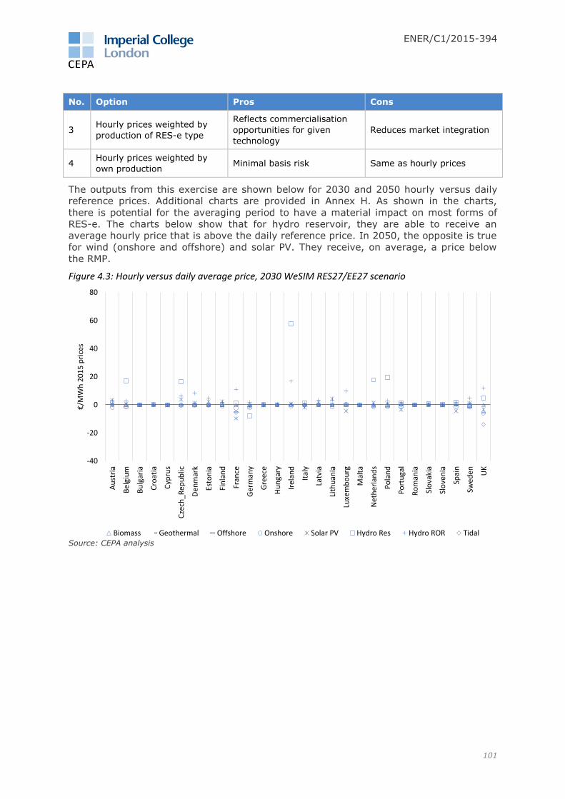
ENER/C1/2015-394

101

No. Option Pros Cons


production of RES-e type

Reflects commercialisation

opportunities for given

technology

Reduces market integration


own production Minimal basis risk Same as hourly prices

The outputs from this exercise are shown below for 2030 and 2050 hourly versus daily

reference prices. Additional charts are provided in Annex H. As shown in the charts,

there is potential for the averaging period to have a material impact on most forms of

RES-e. The charts below show that for hydro reservoir, they are able to receive an

average hourly price that is above the daily reference price. In 2050, the opposite is true

for wind (onshore and offshore) and solar PV. They receive, on average, a price below

the RMP.

Figure 4.3: Hourly versus daily average price, 2030 WeSIM RES27/EE27 scenario


-40

-20

0

20

40

60

80

Au

stri

a

Be

lgiu

m

Bu

lgar

ia

Cro

atia

Cyp

rus

Cze

ch_R

epu

blic

Den

mar

k

Esto

nia

Fin

lan

d

Fran

ce

Ger

man

y

Gre

ece

Hu

nga

ry

Irel

and

Ital

y

Latv

ia

Lith

uan

ia

Luxe

mb

ou

rg

Mal

ta

Net

her

lan

ds

Po

lan

d

Po

rtu

gal

Ro

man

ia

Slo

vaki

a

Slo

ven

ia

Spai

n

Swed

en UK

€/M

Wh

20

15

pri

ces

Biomass Geothermal Offshore Onshore Solar PV Hydro Res Hydro ROR Tidal

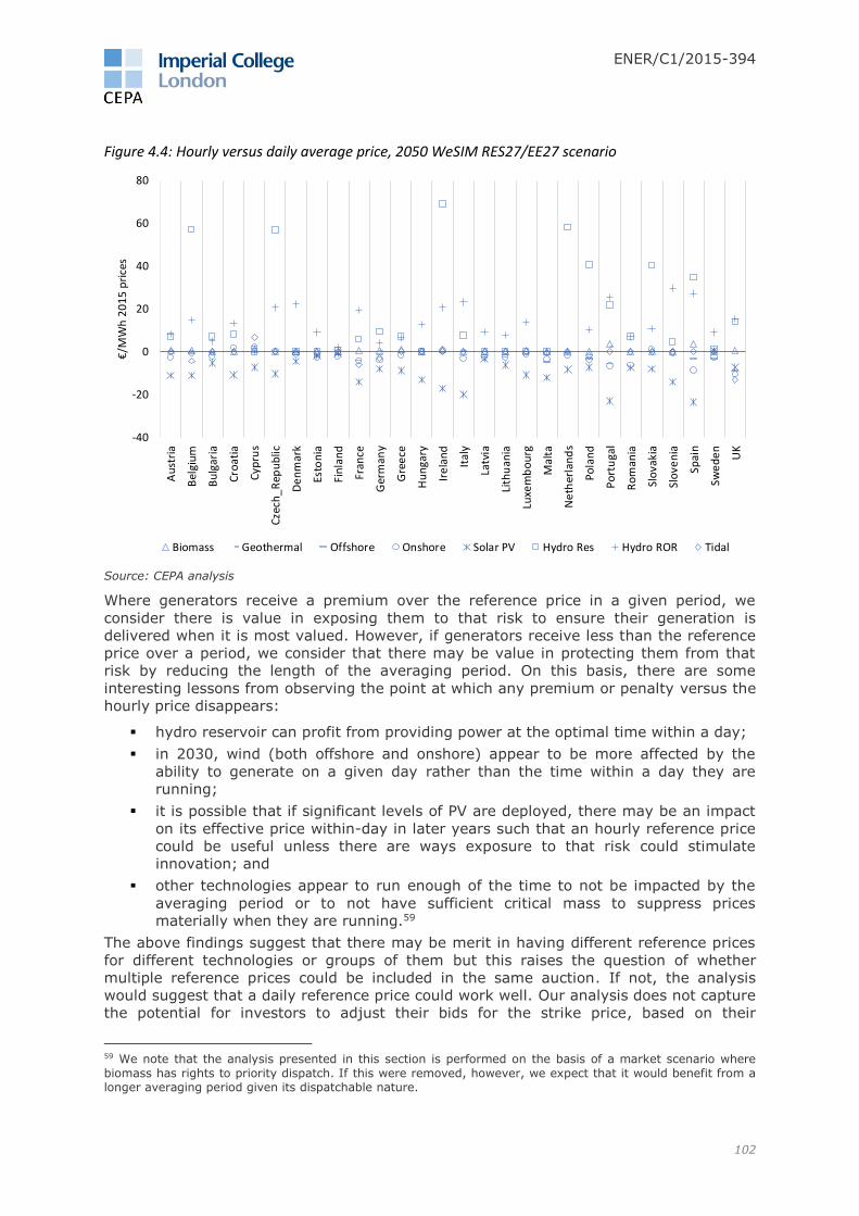
ENER/C1/2015-394

102

Figure 4.4: Hourly versus daily average price, 2050 WeSIM RES27/EE27 scenario


Where generators receive a premium over the reference price in a given period, we

consider there is value in exposing them to that risk to ensure their generation is

delivered when it is most valued. However, if generators receive less than the reference

price over a period, we consider that there may be value in protecting them from that

risk by reducing the length of the averaging period. On this basis, there are some

interesting lessons from observing the point at which any premium or penalty versus the

hourly price disappears:

hydro reservoir can profit from providing power at the optimal time within a day;

in 2030, wind (both offshore and onshore) appear to be more affected by the

ability to generate on a given day rather than the time within a day they are

running;

it is possible that if significant levels of PV are deployed, there may be an impact

on its effective price within-day in later years such that an hourly reference price

could be useful unless there are ways exposure to that risk could stimulate

innovation; and

other technologies appear to run enough of the time to not be impacted by the

averaging period or to not have sufficient critical mass to suppress prices

materially when they are running.59

The above findings suggest that there may be merit in having different reference prices

for different technologies or groups of them but this raises the question of whether

multiple reference prices could be included in the same auction. If not, the analysis

would suggest that a daily reference price could work well. Our analysis does not capture

the potential for investors to adjust their bids for the strike price, based on their

59 We note that the analysis presented in this section is performed on the basis of a market scenario where

biomass has rights to priority dispatch. If this were removed, however, we expect that it would benefit from a longer averaging period given its dispatchable nature.

-40

-20

0

20

40

60

80A

ust

ria

Bel

giu

m

Bu

lgar

ia

Cro

atia

Cyp

rus

Cze

ch_

Rep

ub

lic

De

nm

ark

Esto

nia

Fin

lan

d

Fran

ce

Ger

man

y

Gre

ece

Hu

nga

ry

Ire

lan

d

Ital

y

Latv

ia

Lith

uan

ia

Luxe

mb

ou

rg

Mal

ta

Ne

ther

lan

ds

Po

lan

d

Po

rtu

gal

Ro

man

ia

Slo

vaki

a

Slo

ven

ia

Spai

n

Swe

de

n

UK

€/M

Wh

20

15

pri

ces


ENER/C1/2015-394

103

expectation of earning more or less than the reference price. For example, the potential

to profitably outperform the MRP might allow some generators to reduce their strike

price bids. We could also expect the opposite behaviour from generators that typically

earn prices below the reference price.

It is important to note that the analysis presented above is based on fixed generation

profiles for each hour of the year estimated on the basis of generators responding to

hourly price signals and therefore does not demonstrate the impact of the averaging

period on their decision of when to generate.

ENER/C1/2015-394

104

5 Quantitative assessment of policy options Having established estimates of the investment gap, described in Section 3.3, in this

section we consider the quantitative impact of the policy options presented in Section 4.

First, we summarise, at a high level, the approach to our quantitative assessment of the

RES-e support options. As shown in Figure 5.1, our quantification focuses on establishing

the funding gap and how policy options can influence the cost of support.

Figure 5.1: Funding gap assessment approach

Each support option may result in a different profile of revenues for generators, but also

their overall risk. All else being equal, support options that reduce risk for generators, in

a way that reduces their investors’ discount rates, have the potential to reduce the

overall cost of support.

Next, we set out our approach to estimating discount rates for each support option, and

also present our estimates. Using those estimates, we go on to present the findings

regarding the cost of support for each policy option, which inform our qualitative

assessment of those options.

5.1 Discount rates

In this section, we present our approach to estimating the discount rates used in this

study. We briefly explain their role and the values used, and then identify the

dimensions captured in our analysis, as well as the approach used to capture them.

Further detail on our analysis is provided in Annex C.

5.1.1 Discount rates, cost of capital and hurdle rates

Alongside estimates of capex and wholesale market revenues, discount rates are an

input into our viability gap modelling. In simple terms, the discount rate’s role is to put

cashflows that are earned at different points in time on a comparable basis. This

calculation is performed from the point of view of an investor deciding if it should go

ahead with a new project. For this reason, we use whole-life commercial values.60 As we

forecast cashflows in our viability analysis on a real basis, and since we do not

separately forecast tax, we use real pre-tax discount rates.

60 We do not, for example, consider separate discount rates for the project development and post-construction stages of the project life. For further discussion of this see p7, CEPA (2011).

Discount rateby support option

Scenario

Cost of supportby support option

Discount rateEOM only

MWh eligible for support

Support level

Output

Calculation

Input

Key

Geog. scope

ENER/C1/2015-394

105

The cost of capital is one value that can be used as the discount rate.61 Practitioners

often estimate this using a weighted average cost of capital (WACC) framework, relying

on the capital asset pricing model (CAPM) to estimate the cost of equity component.62

Such models are powerful, but quite focused on the volatility of cashflows, making them

most appropriate when applied to cashflow forecasts based on probability-weighted

estimates. For example, if there were a 99 percent chance that revenue in a given period

could be €100.00 and a 1 percent chance it could be €50.00, the probability-weighted

expected value would be €99.50.

In cases where it is not possible to calculate such rich forecasts as a purist cost of capital

approach might demand, it is reasonable to expect an investor to aim up (or down) from

their cost of capital to capture the expectation of cashflows on balance being worse, or

better, than the cashflows indicate. Such a rate would be considered a “hurdle rate”.

Building on the example in the paragraph above, if the investor was solely to use the

most likely value of €100, they could attempt to capture the downside risk by applying a

higher discount rate. If the revenue were to be received one year in the future, and the

cost of capital were 10.00 percent, an equivalent present value could be achieved by

using a discount rate of 10.55 percent, 55 basis points higher than if the risk had already

been captured in the cashflows. This approach is less elegant but may better reflect how

projects are actually assessed in practice.

While we have a cost of capital methodology at the heart of our analysis, we consider it

most accurate to describe our discount rate estimates as hurdle rates.63 We consider this

to be consistent with our approach to viability modelling, and also with our reading of

the broader literature from which we drew comparator values to inform the analysis.64

5.1.2 Approach

The objective of our discount rate analysis was to produce estimates:

1. based on deployment dates in 2020, 2025, 2030, 2040 and 2050;65

2. for each of the EU 28 MS;

3. for a set of RES-e technologies included in our viability modelling;

4. with wholesale market revenues only and under a set of primary support

mechanisms; and

5. with auxiliary support options.66

Our calculations capture these five dimensions. They are based on a combination of

bottom-up cost of capital estimates, calibrated using structured relative risk analysis and

top-down evidence on hurdle rates. The bottom-up cost of capital analysis allowed us to

produce estimates that capture the variation in the cost of capital over time and by

location. It also allowed for a more targeted approach to quantifying the impact of

61 One alternative option, used for example to assess the value for money of government policy interventions, is the “social” discount rate defined on a non-commercial basis. 62 The WACC is a weighted average of the cost of debt and the cost of equity. While the cost of debt can be observed, the cost of equity cannot, necessitating the use of models such as the CAPM. 63 This approach is in line with similar studies based in the UK. For example, see Section 2.2 of NERA (Dec 2013) “Changes in Hurdle Rates for Low Carbon Generation Technologies due to the Shift from the UK Renewables Obligation to a Contracts for Difference Regime” available on the GOV.UK website here and Sections 2.1 and 2.2. of Oxera (Apr 2011) “Discount rates for low-carbon and renewable generation technologies” available on the CCC website here. 64 We would for example characterise the cost of capital values presented in DiaCore (2016) to be hurdle rates. 65 Note: we use an annual model that assumes that construction is completed in the year stated, with the first year of production being in the following year. 66 We also considered how the cost of capital might vary between the different electricity market scenarios developed in Task 2. We decided, however, to focus on the five dimensions noted above as they were expected

to be more amenable to quantification and potentially of more material impact. This dimension was, however, considered qualitatively in the Task 4 Finance Workshop.

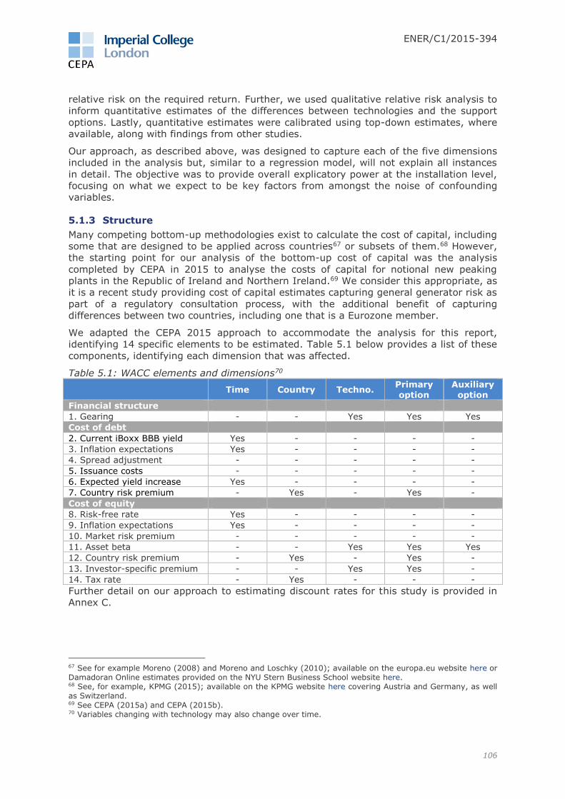
https://www.gov.uk/government/uploads/system/uploads/attachment_data/file/267650/NERA_Report_Assessment_of_Change_in_Hurdle_Rates_-_FINAL.pdf

https://www.theccc.org.uk/archive/aws/Renewables%20Review/Oxera%20low%20carbon%20discount%20rates%20180411.pdf

ENER/C1/2015-394

106

relative risk on the required return. Further, we used qualitative relative risk analysis to

inform quantitative estimates of the differences between technologies and the support

options. Lastly, quantitative estimates were calibrated using top-down estimates, where

available, along with findings from other studies.

Our approach, as described above, was designed to capture each of the five dimensions

included in the analysis but, similar to a regression model, will not explain all instances

in detail. The objective was to provide overall explicatory power at the installation level,

focusing on what we expect to be key factors from amongst the noise of confounding

variables.

5.1.3 Structure

Many competing bottom-up methodologies exist to calculate the cost of capital, including

some that are designed to be applied across countries67 or subsets of them.68 However,

the starting point for our analysis of the bottom-up cost of capital was the analysis

completed by CEPA in 2015 to analyse the costs of capital for notional new peaking

plants in the Republic of Ireland and Northern Ireland.69 We consider this appropriate, as

it is a recent study providing cost of capital estimates capturing general generator risk as

part of a regulatory consultation process, with the additional benefit of capturing

differences between two countries, including one that is a Eurozone member.

We adapted the CEPA 2015 approach to accommodate the analysis for this report,

identifying 14 specific elements to be estimated. Table 5.1 below provides a list of these

components, identifying each dimension that was affected.

Table 5.1: WACC elements and dimensions70

Time Country Techno. Primary

option

Auxiliary

option

Financial structure

1. Gearing - - Yes Yes Yes

Cost of debt

2. Current iBoxx BBB yield Yes - - - -

3. Inflation expectations Yes - - - -

4. Spread adjustment - - - - -

5. Issuance costs - - - - -

6. Expected yield increase Yes - - - -

7. Country risk premium - Yes - Yes -

Cost of equity

8. Risk-free rate Yes - - - -

9. Inflation expectations Yes - - - -

10. Market risk premium - - - - -

11. Asset beta - - Yes Yes Yes

12. Country risk premium - Yes - Yes -

13. Investor-specific premium - - Yes Yes -

14. Tax rate - Yes - - -

Further detail on our approach to estimating discount rates for this study is provided in

Annex C.

67 See for example Moreno (2008) and Moreno and Loschky (2010); available on the europa.eu website here or Damadoran Online estimates provided on the NYU Stern Business School website here. 68 See, for example, KPMG (2015); available on the KPMG website here covering Austria and Germany, as well as Switzerland. 69 See CEPA (2015a) and CEPA (2015b). 70 Variables changing with technology may also change over time.

http://publications.jrc.ec.europa.eu/repository/bitstream/JRC57880/consolidated%20indicator%20-%20final%20-%20version%202010-04-09.pdf

http://people.stern.nyu.edu/adamodar/New_Home_Page/data.html

https://assets.kpmg.com/content/dam/kpmg/pdf/2016/01/kpmg-cost-of-capital-study-2015.pdf

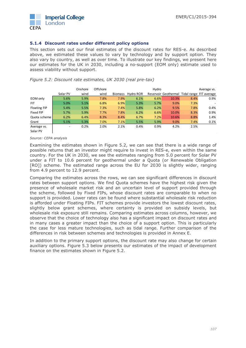
ENER/C1/2015-394

107

5.1.4 Discount rates under different policy options

This section sets out our final estimates of the discount rates for RES-e. As described

above, we estimated these values to vary by technology and by support option. They

also vary by country, as well as over time. To illustrate our key findings, we present here

our estimates for the UK in 2030, including a no-support (EOM only) estimate used to

assess viability without support.

Figure 5.2: Discount rate estimates, UK 2030 (real pre-tax)


Examining the estimates shown in Figure 5.2, we can see that there is a wide range of

possible returns that an investor might require to invest in RES-e, even within the same

country. For the UK in 2030, we see the estimates ranging from 5.0 percent for Solar PV

under a FIT to 10.6 percent for geothermal under a Quota (or Renewable Obligation

[RO]) scheme. The estimated range across the EU for 2030 is slightly wider, ranging

from 4.9 percent to 12.9 percent.

Comparing the estimates across the rows, we can see significant differences in discount

rates between support options. We find Quota schemes have the highest risk given the

presence of wholesale market risk and an uncertain level of support provided through

the scheme, followed by Fixed FIPs, whose discount rates are comparable to when no

support is provided. Lower rates can be found where substantial wholesale risk reduction

is afforded under Floating FIPs. FIT schemes provide investors the lowest discount rates,

slightly below grant schemes, where certainty is provided on subsidy levels, but

wholesale risk exposure still remains. Comparing estimates across columns, however, we

observe that the choice of technology also has a significant impact on discount rates and

in many cases a greater impact than the choice of a support option. This is particularly

the case for less mature technologies, such as tidal range. Further comparison of the

differences in risk between schemes and technologies is provided in Annex E.

In addition to the primary support options, the discount rate may also change for certain

auxiliary options. Figure 5.3 below presents our estimates of the impact of development

finance on the estimates shown in Figure 5.2.

Solar PV

Onshore

wind

Offshore

wind Biomass Hydro ROR

Hydro

Reservoir Geothermal Tidal range

Average vs.

FIT average

EOM only 5.6% 5.9% 7.8% 7.9% 6.1% 6.6% 10.3% 8.4% 0.9%

FIT 5.0% 5.1% 6.8% 6.9% 5.3% 5.7% 9.0% 7.3% -

Floating FIP 5.4% 5.5% 7.3% 7.4% 5.8% 6.2% 9.5% 7.8% 0.4%

Fixed FIP 5.7% 5.9% 7.7% 7.8% 6.2% 6.6% 10.0% 8.3% 0.9%

Quota scheme 6.2% 6.4% 8.3% 8.4% 6.7% 7.2% 10.6% 8.8% 1.4%

Grant 5.1% 5.3% 7.0% 7.1% 5.5% 5.9% 9.0% 7.4% 0.1%

Average vs.

Solar PV

- 0.2% 2.0% 2.1% 0.4% 0.9% 4.2% 2.5%

ENER/C1/2015-394

108

Figure 5.3: Development finance impact estimates, UK 2030 (real pre-tax)

Lower scenario (5 ppt increase in gearing)

Higher scenario (10 ppt increase in gearing)


As evident in Figure 5.3, we have limited our analysis of development finance to cases

where the RES-e technology is large in scale or not yet mature: offshore wind and hydro

reservoir given their scale, and geothermal and tidal range on grounds of maturity.71

Where available, this option has the potential to reduce the discount rate for a

technology substantially. For example, our estimates indicate the potential amounts to

more than half the difference in discount rates between offshore and onshore wind. That

said, this option is likely be of greatest benefit in countries where investment conditions

are less favourable, particularly where the availability of development finance enables

projects to become bankable, rather than simply reducing the cost of finance for projects

that are already able to secure debt.

We find that the ability for development finance to influence the viability of a project is

affected by the adopted primary support scheme. Lower-risk primary support schemes,

such as a Floating FIP, allow greater participation of debt finance. This increases the

base over which development finance can have its effect. Therefore, the impact of

development finance increases as the primary support scheme risk declines.

Figure 5.4 presents the impact of another auxiliary policy option, carbon contracting, on

discount rates, compared to those shown in Figure 5.2.

Figure 5.4: Carbon contracting impact estimates, UK 2030 (real pre-tax)


71 We note that, based on its forecast path to maturity, we permitted development finance in our modelling for biomass in 2020 and 2025 but assumed it would not be necessary from 2030 onwards.

Solar PV

Onshore

wind

Offshore


Hydro


EOM only -0.2% -0.2% -0.3% -0.2%

FIT -0.5% -0.2% -0.6% -0.4%

Floating FIP -0.5% -0.3% -0.6% -0.4%

Fixed FIP -0.4% -0.3% -0.5% -0.4%

Quota scheme -0.4% -0.3% -0.5% -0.4%

Grant -0.8% -0.4% -0.8% -0.6%

Solar PV

Onshore

wind

Offshore


Hydro


EOM only -0.5% -0.3% -0.7% -0.5%

FIT -1.0% -0.5% -1.2% -0.8%

Floating FIP -1.0% -0.5% -1.2% -0.8%

Fixed FIP -0.9% -0.5% -1.1% -0.8%

Quota scheme -0.9% -0.6% -1.1% -0.8%

Grant -1.7% -0.7% -1.7% -1.1%

Solar PV

Onshore

wind

Offshore


Hydro


EOM only -0.21% -0.22% -0.22% -0.22% -0.22% -0.22% -0.23% -0.23%

FIT

Floating FIP

Fixed FIP -0.20% -0.20% -0.20% -0.20% -0.20% -0.21% -0.21% -0.21%

Quota scheme -0.20% -0.20% -0.20% -0.20% -0.20% -0.21% -0.21% -0.21%

Grant -0.18% -0.19% -0.19% -0.19% -0.19% -0.19% -0.20% -0.20%

ENER/C1/2015-394

109

Our analysis of carbon contracting finds that there is a potential to reduce discount

rates, but only in cases where substantial wholesale risk protection is not already

provided, such as with a FIT or Floating FIP. Given the impact of wholesale risk across

the entire capital base, we see only limited variations in impacts across technologies or

support schemes.

Given the relatively low risk profile of the UK, we do not identify a cost of capital benefit

from implementation of a regional or EU-wide support scheme. However, we do find

some impact in countries that investors see to be riskier, with potential benefits

estimated for countries with sovereign ratings of AA or lower from 2020 onwards, which

includes 20 MS. For one of those MS, Cyprus, Figure 5.5 below shows the discount rate

improvement for three support options if implemented on an EU-wide basis.

Figure 5.5: EU implementation impact estimates, Cyprus 2020 (real pre-tax)


As can be seen in Figure 5.5, we find the impact of EU-wide implementation to have an

impact that varies little by technology or support scheme. However, as we expect

current differences in country risk to converge from current to longer-term levels over

the next decade, through deeper financial market integration and resolution of ongoing

financial market stresses affecting certain MS, we expect the benefits to project risk to

diminish over time.

5.2 Estimated cost of RES-e support

In this section, we present our findings on the cost of support, which were used to

inform our qualitative assessment of policy options. First, we briefly set out our approach

to deriving cost estimates. Next, we present values for the funding gap and the total cost

of support for the primary and the auxiliary options, assuming national implementation.

We also present estimates for EU-wide implementation of Floating FIP, Fixed FIP and

Quota schemes, as well as the results for the potential impact of regional cooperation.

5.2.1 Approach

As an illustration of our approach to estimating the cost of support, Figure 5.6 below

presents an adapted version of the WeSIM RES27/EE27 “supply curve” shown as Figure

3.17 earlier in the report.

Solar PV

Onshore

wind

Offshore


Hydro


Floating FIP -0.29% -0.30% -0.30% -0.30% -0.30% -0.30% -0.31% -0.31%

Fixed FIP -0.30% -0.30% -0.31% -0.31% -0.30% -0.31% -0.32% -0.32%

Quota scheme -0.30% -0.30% -0.31% -0.31% -0.31% -0.31% -0.32% -0.32%

ENER/C1/2015-394

110

Figure 5.6: RES-e curtailed supply curves under (WeSIM RES27/EE27, 2020)


Three changes were made to the curves in Figure 3.17 to generate Figure 5.6:

1. projects viable without support were excluded, truncating the original “no

support” curve at the point where it crosses the horizontal axis;

2. for the remaining projects, viability gaps were recalculated using the discount

rate for each support option, resulting in the shifted “Floating FIP” curve shown

above; and

3. the resulting viability gaps were expressed in €/MWh (in 2015 prices) over the

assumed life of the support scheme (15 years), instead of the full technology-

specific asset life; this approximates the way clearing bid prices for support would

be determined in a competitive allocation mechanism.

Following these three steps, the area between each curve and the horizontal axis can be

interpreted as a measure of the total funding gap for the first year of each scheme. This

first-year funding gap is projected over the life of the projects to estimate the overall

“funding gap” and the “total cost of support”.

The “funding gap” represents the cost of support when technology-specific schemes are

implemented in each country, assuming the scheme administrator is able to perfectly

price discriminate between different RES-e technologies. As we do not consider this

feasible on the scale of the investment challenge,72 we adopted a technology-neutral

approach for most options in this study. As such, we estimate the “total cost of support”

72 For example, scheme administrators might attempt to use pay-as-bid auctions to price discriminate;

however, they are likely to lead to strategic bidding, as RES-e investors would have little incentive to reveal their true costs.

-50

0

50

100

150

200

250

300

0 2 4 6 8 10 12 14 16

€/M

Wh

20

15

pri

ces

Production in TWh

Floating FIP No support

ENER/C1/2015-394

111

by first identifying the marginal RES-e within the geographic scope of each scheme to

set the level of support provided to all participating generators.73

The total funding gap is affected primarily by two factors:

Viability gaps of RES-e—only technologies that are not viable without support

will contribute to the funding gap. Individual RES-e viability gaps are determined

by generator-specific revenues and costs. Revenues differ across scenarios due to

differences in wholesale electricity prices and total generation, while costs vary by

scenario (due to total generation) and by support option (due to differences in the

respective discount rates).

Investment volumes—more deployment of non-viable RES-e translates directly

into a larger quantum of MWh that need to be subsidised; thus investment

volumes vary across scenarios.

As discussed earlier, we assumed that uniform-price auctions set the level of support for

most options, and therefore the total cost of support must be at least as large as the

funding gap. The next section presents our results, assuming national implementation of

the support options. As with the funding gap, the total cost of support is affected by

individual RES-e viability gaps and the overall investment challenge. In addition, the

total cost of support also depends on the viability gap of the least-viable RES-e

technology that needed in each country to achieve renewables targets.

5.2.2 Results: National implementation

In this section, we present estimates of the funding gap and the total cost of support,

assuming that support schemes are implemented at the MS level.

With national implementation, we assumed that each MS would hold a competitive

auction for the chosen support mechanism. We modelled these as “closed” auctions,

such that only generators physically located within the borders of the MS could

participate, and technology eligibility determined based on a country-by-country

assessment of viability without support.

The estimates presented are expressed in net present value terms, discounted using the

corresponding discount rates, as described in Section 5.1. For our analysis of the total

cost of support, we assumed that neither tidal range nor biomass would set the subsidy

level. Specifically, it is likely that competitive RES-e auctions would attract additional

lower-cost RES-e capacity, such as solar PV and offshore wind, and relatively expensive

RES-e technologies would only clear if no lower-cost option were available to fulfil the

RES-e targets.74

In the following two sections we present estimates of the funding gap for primary

options and auxiliary options. Note that each figure showing the funding gap for a given

period (e.g., between 2020 and 2030) should be interpreted as the annual funding gap

for RES-e that is installed within that period.75

Funding gap for primary options

For our central scenario, WeSIM RES27/EE27, we estimate that the funding gap between

2020 and 2030 is between €32 billion and €44 billion (2015 prices) depending on the

primary support option chosen, shown in Figure 5.7. Although this a fairly wide range of

73 We assume that technologies viable without support are excluded from the auction. 74 PRIMES scenarios include some relatively expensive RES-e technologies in their deployment projections in order to reflect current Member States' support and policies for a range of RES-e technologies. 75 Please note that the financial modelling conducted as part of this study was conducted at an annual

resolution. Therefore, for clarity, please note that in this study, the period 2020-2030 is one decade long and the period 2020-2050 is three decades long.

ENER/C1/2015-394

112

estimates, the greatest differences are primarily driven by market scenario, not policy

option.

Across the scenarios, we see one of the largest funding gaps emerging in the WeSIM

RES27/EE Pessimistic scenario, which was constructed to represent unfavourable market

conditions for RES-e. The relatively high cost for WeSIM RES27/EE Pessimistic scenario

is therefore to be expected, since, as we discussed in Section 3.3.2, the WeSIM

RES27/EE Pessimistic scenario had relatively low wholesale prices compared to other

scenarios. This in turn, translated into larger viability gaps for RES-e, which directly

increased the overall funding gap.

The WeSIM RES27/EE30 and WeSIM RES30/EE30 scenarios results in funding gaps

similar to that of the WeSIM RES27/EE Pessimistic scenario, and are about double that of

the WeSIM RES27/EE27 scenario. This is in part due to a relatively high volume of

projects being built (i.e., there is a larger investment challenge) between 2020 and 2030

in these scenarios compared with WeSIM RES27/EE27. This is visible in the 2020 supply

curve shown Figure 3.17, which is shifted to the right, compared with the supply curve

for the WeSIM RES27/EE27 scenario. In particular, the WeSIM RES27/EE30 scenario has

more offshore wind and solar PV capacity installed in those years. As a result, the total

volume of RES-e that requires support is higher.

When extending the time horizon to consider the funding gap for all RES-e projects

installed between 2020 and 2050, shown in Figure 5.8, we see the largest deviation from

the other primary options for the WeSIM RES27/EE Pessimistic scenario. This finding is a

product of a number of assumptions used in that scenario to represent unfavourable

market conditions. They include lower ETS prices, reduced interconnection capacity and

lower DSR penetration, and together depress wholesale prices, resulting in larger

viability gaps for RES-e.

ENER/C1/2015-394

113

Figure 5.7: Funding gap in €bn (2015 prices) between 2020 and 2030 by scenario


Figure 5.8: Funding gap in €bn (2015 prices) between 2020 and 2050 by scenario


The results of our sensitivity analysis, in which we varied only one parameter relative to

the WeSIM RES27/EE27 scenario, are shown in the following two charts, Figure 5.9 and

€ -

€ 10

€ 20

€ 30

€ 40

€ 50

€ 60

€ 70

€ 80


Sup

po

rt r

eq

uir

ed

(€

bn

20

15

pri

ces)

WeSIM RES27/EE27


WeSIM RES27/EE30

WeSIM RES30/EE30

WeSIM Ref

€ -

€ 50

€ 100

€ 150

€ 200

€ 250

€ 300


Sup

po

rt r

eq

uir

ed

(€

bn

20

15

pri

ces)

WeSIM RES27/EE27


WeSIM RES27/EE30

WeSIM RES30/EE30

WeSIM Ref

ENER/C1/2015-394

114

Figure 5.10 for the periods 2020-2030 and 2020-2050, respectively.76 Not surprisingly,

sensitivities, which introduce higher costs or lower market revenues, result in a larger

funding gap, due to increased project-level viability gaps. This is the case for the

discount rate based sensitivities, ETS sensitivity and the sensitivity assuming investor

myopia over future ETS prices. In contrast to those cases, the sensitivity with more

aggressive offshore wind cost reductions reduces the viability gaps for that technology,

resulting in correspondingly lower funding gaps.

Comparing Figure 5.9 and Figure 5.10, we can see that the impact of the Lower ETS and

Imperfect foresight scenarios become larger over time. Over the longer period, the

impact of the Lower ETS scenario moves from being comparable to a 100 basis point

increase in discount rates to being the most costly sensitivity. In the earlier period, the

Imperfect foresight scenario has the largest funding gap of the scenarios considered,

highlighting the importance of policy credibility and how it can deliver cost savings to

electricity customers. The relative deterioration in cost over the period, however, is not

as large as for the Lower ETS sensitivity as in the later years, as we assume investors to

have factored prior baseline ETS increases into their forecasts.

To put these sensitivity results in context, comparing Figures 5.8 and5.10, we can see

that the magnitude of impact of the Lower ETS scenario is only exceeded by the WeSIM

RES27/EE Pessimistic scenario, which itself can almost be interpreted as a combined

sensitivity of unfavourable market developments. Ultimately, these findings suggest that

the cost of RES support will be highly influenced by the success (or failure) of other non-

RES policies, but also that improving the credibility of reforms is of significant value to

electricity customers.

76 We note that in addition to the sensitivity analysis presented here, WeSIM RES27/EE Pessimistic scenario presented above could be interpreted as a form of a combined sensitivity.

ENER/C1/2015-394

115

Figure 5.9: Funding gap in €bn (2015 prices) between 2020 and 2030 by sensitivity


€ -

€ 10

€ 20

€ 30

€ 40

€ 50

€ 60

€ 70


Sup

po

rt r

eq

uir

ed

(€b

n 2

01

5 p

rice

s)

WeSIM RES27/EE27

Lower ETS

National CRMs

WACC +1%

WACC +2%

Low offshore costs

Imperfect foresight

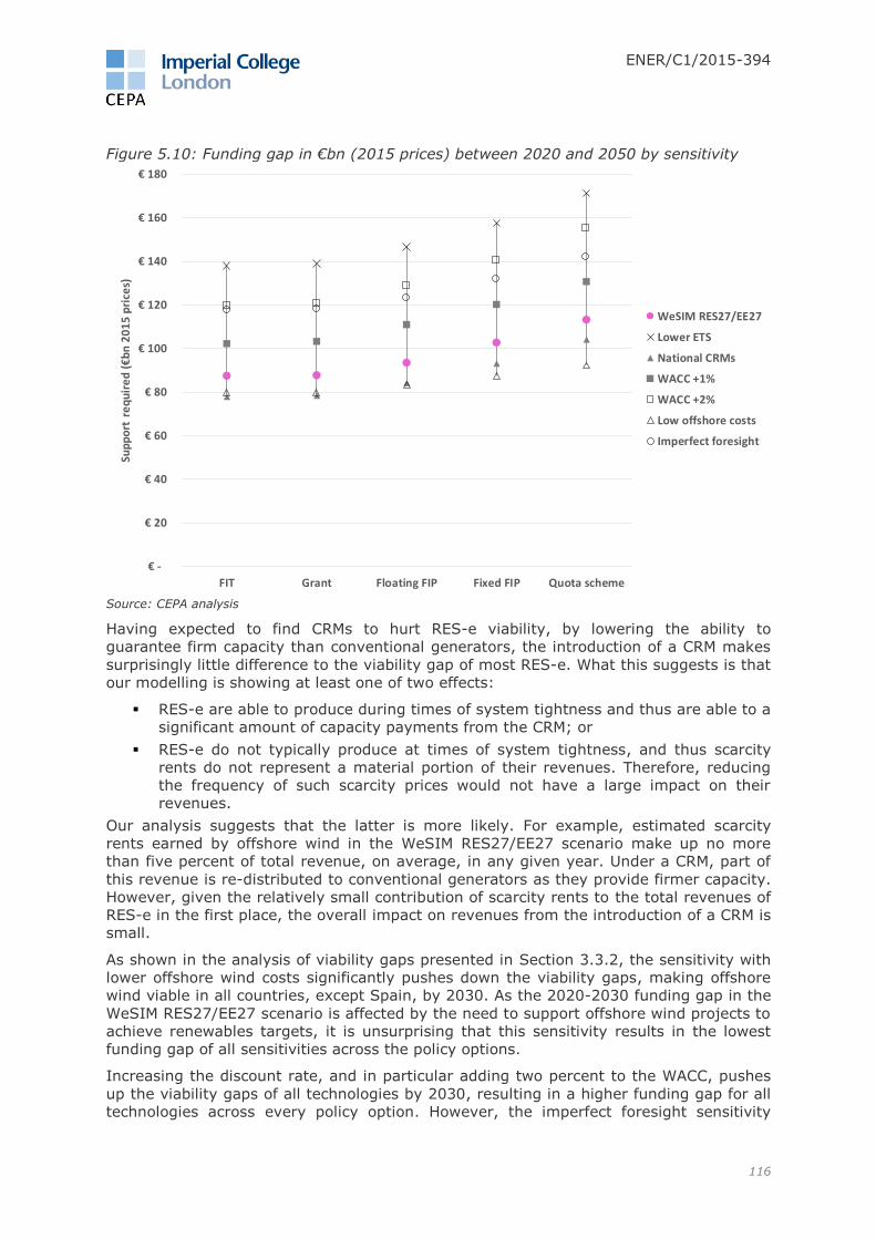
ENER/C1/2015-394

116

Figure 5.10: Funding gap in €bn (2015 prices) between 2020 and 2050 by sensitivity


Having expected to find CRMs to hurt RES-e viability, by lowering the ability to

guarantee firm capacity than conventional generators, the introduction of a CRM makes

surprisingly little difference to the viability gap of most RES-e. What this suggests is that

our modelling is showing at least one of two effects:

RES-e are able to produce during times of system tightness and thus are able to a

significant amount of capacity payments from the CRM; or

RES-e do not typically produce at times of system tightness, and thus scarcity

rents do not represent a material portion of their revenues. Therefore, reducing

the frequency of such scarcity prices would not have a large impact on their

revenues.

Our analysis suggests that the latter is more likely. For example, estimated scarcity

rents earned by offshore wind in the WeSIM RES27/EE27 scenario make up no more

than five percent of total revenue, on average, in any given year. Under a CRM, part of

this revenue is re-distributed to conventional generators as they provide firmer capacity.

However, given the relatively small contribution of scarcity rents to the total revenues of

RES-e in the first place, the overall impact on revenues from the introduction of a CRM is

small.

As shown in the analysis of viability gaps presented in Section 3.3.2, the sensitivity with

lower offshore wind costs significantly pushes down the viability gaps, making offshore

wind viable in all countries, except Spain, by 2030. As the 2020-2030 funding gap in the

WeSIM RES27/EE27 scenario is affected by the need to support offshore wind projects to

achieve renewables targets, it is unsurprising that this sensitivity results in the lowest

funding gap of all sensitivities across the policy options.

Increasing the discount rate, and in particular adding two percent to the WACC, pushes

up the viability gaps of all technologies by 2030, resulting in a higher funding gap for all

technologies across every policy option. However, the imperfect foresight sensitivity

€ -

€ 20

€ 40

€ 60

€ 80

€ 100

€ 120

€ 140

€ 160

€ 180


Sup

po

rt r

eq

uir

ed

(€b

n 2

01

5 p

rice

s)

WeSIM RES27/EE27

Lower ETS

National CRMs

WACC +1%

WACC +2%

Low offshore costs

Imperfect foresight

ENER/C1/2015-394

117

generates the highest funding gap between 2020 and 2030 for certain policy options.

This is consistent with our finding that the principle drivers of changes in the viability gap

are expected revenues rather than the LCOE, and that one of the key drivers of

wholesale prices is the carbon price. Given this scenario assumes investors forecast low

ETS prices, this sensitivity yields lower market prices, a higher viability gap at the

project level, and thus a higher funding gap overall.

These results suggest that the main drivers of the viability gap are the cost of capital

and the evolution of electricity prices. If the discount rates are higher due to an

increased perception of risks by investors, then viability gaps increase, resulting in a

higher funding gap. Similarly, lower expectations regarding future electricity prices

increase the funding gap for all technologies.

We performed an additional sensitivity that assumes the removal of priority dispatch for

all generators. Priority dispatch is a market access rule, which gives priority to energy

generated by RES-e over conventional generation. In our modelling, this was most

relevant for biomass since other RES-e generators are assumed to have zero (or near

zero) marginal costs. Giving biomass priority dispatch effectively pushes down the

electricity price, since biomass becomes a price-taker, replacing other conventional

generators. Therefore, in terms of overall viability, we find that priority dispatch on its

own would be detrimental to RES-e viability. Results for the funding gap are shown in

Figure 5.11 and Figure 5.12. Funding gaps in the WeSIM RES27/EE27 scenario (with

priority dispatch for biomass) were higher, compared to the case where priority dispatch

is removed. The impact of priority dispatch on the total cost of support is not as

straightforward, and is explained below in Section 5.2.2.

Figure 5.11: Funding gap in €bn (2015 prices) between 2020 and 2030


€ -

€ 5

€ 10

€ 15

€ 20

€ 25

€ 30

€ 35

€ 40

€ 45

€ 50


Sup

po

rt r

eq

uir

ed

(€b

n 2

01

5 p

rice

s)

WeSIM RES27/EE27

No pref rules

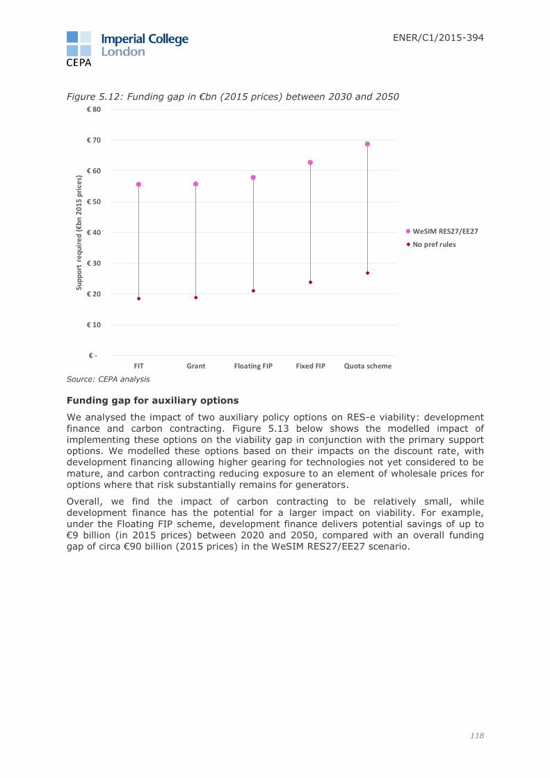
ENER/C1/2015-394

118

Figure 5.12: Funding gap in €bn (2015 prices) between 2030 and 2050


Funding gap for auxiliary options

We analysed the impact of two auxiliary policy options on RES-e viability: development

finance and carbon contracting. Figure 5.13 below shows the modelled impact of

implementing these options on the viability gap in conjunction with the primary support

options. We modelled these options based on their impacts on the discount rate, with

development financing allowing higher gearing for technologies not yet considered to be

mature, and carbon contracting reducing exposure to an element of wholesale prices for

options where that risk substantially remains for generators.

Overall, we find the impact of carbon contracting to be relatively small, while

development finance has the potential for a larger impact on viability. For example,

under the Floating FIP scheme, development finance delivers potential savings of up to

€9 billion (in 2015 prices) between 2020 and 2050, compared with an overall funding

gap of circa €90 billion (2015 prices) in the WeSIM RES27/EE27 scenario.

€ -

€ 10

€ 20

€ 30

€ 40

€ 50

€ 60

€ 70

€ 80


Sup

po

rt r

eq

uir

ed

(€b

n 2

01

5 p

rice

s)

WeSIM RES27/EE27

No pref rules

ENER/C1/2015-394

119

Figure 5.13: Savings from development finance and carbon contracting on primary

support funding gap between 2020 and 2050 in €bn (2015 prices)


Total cost of support for primary options

Total cost of support for the primary policy options are presented for 2020-2030 and

2020-2050 in Figure 5.14 and Figure 5.15, respectively. As was the case for the funding

gap, the total cost of support for projects installed between 2020 and 2030 is the highest

under the WeSIM RES27/EE Pessimistic and WeSIM RES27/EE30 scenarios.

We find that the WeSIM Ref scenario has a relatively low total cost of support, compared

to other scenarios. This is the result of several factors, including the fact that with lower

RES-e penetration there are fewer projects requiring support. Lower RES-e penetration

also means that the cannibalisation effect, discussed in Section 3, is weaker, leading to

relatively high wholesale prices.

€ -

€ 2

€ 4

€ 6

€ 8

€ 10

€ 12

€ 14

€ 16


Re

du

ctio

n i

n s

up

po

rt r

eq

uir

ed

(€b

n 2

01

5 p

rice

s)

Development finance (high)

Development finance (low)

Carbon contracting

ENER/C1/2015-394

120

Figure 5.14: Total cost of support in €bn (2015 prices) between 2020 and 2030 by

scenario



scenario


We observed similar trends in the viability gap under the sensitivity scenarios. Figure

5.16 and Figure 5.17 show the total cost of support by policy option and sensitivity for

€ -

€ 20

€ 40

€ 60

€ 80

€ 100

€ 120


Sup

po

rt r

ece

ive

d (€

bn

20

15

pri

ces)

WeSIM RES27/EE27


WeSIM RES27/EE30

WeSIM RES30/EE30

WeSIM Ref

€ -

€ 50

€ 100

€ 150

€ 200

€ 250

€ 300

€ 350


Sup

po

rt r

ecei

ved

(€

bn

20

15

pri

ces)

WeSIM RES27/EE27


WeSIM RES27/EE30

WeSIM RES30/EE30

WeSIM Ref

ENER/C1/2015-394

121

2020-2030 and 2020-2050, respectively. Again, sensitivities that involve a higher cost of

capital or lower expected future prices lead to higher subsidy requirements due to higher

viability gaps across all RES-e. As for the funding gap, CRMs appear to have little impact

on the total cost of support for the same reasons discussed previously (i.e., scarcity

rents contribute to a relatively small portion of overall RES-e revenues).

WACC sensitivities increase the viability gaps for all technologies, including the viability

gap of the marginal technology that sets the support levels. This explains the large

spread between the WACC+2% sensitivity and the WeSIM RES27/EE27 scenario. As

explained above, lower ETS prices lower the levelised revenues, and therefore increase

the viability gaps for all types of RES-e.

The only sensitivity that has a positive impact on the total cost of support is the offshore

wind sensitivity, reflecting the high share of non-viable offshore projects that require

support between 2020 and 2030. Furthermore, this also tells us that offshore wind sets

the support level in some countries/years, meaning that it is one of the most expensive

technologies installed.


sensitivity (except non-priority dispatch)


€ -

€ 10

€ 20

€ 30

€ 40

€ 50

€ 60

€ 70

€ 80

€ 90


Sup

po

rt r

ece

ive

d (€

bn

20

15

pri

ces)

WeSIM RES27/EE27

Lower ETS

National CRMs

WACC +1%

WACC +2%

Low offshore costs

Imperfect foresight

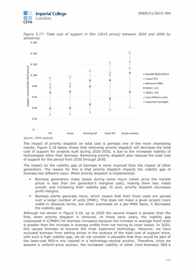
ENER/C1/2015-394

122


sensitivity


The impact of priority dispatch on total cost is perhaps one of the more interesting

results. Figure 5.18 below shows that removing priority dispatch will decrease the total

cost of support for projects built during 2020-2030, a due to the increased viability of

technologies other than biomass. Removing priority dispatch also reduces the total cost

of support for the period from 2030 through 2050.

The impact on the viability gap of biomass is more nuanced than the impact of other

generators. The reason for this is that priority dispatch impacts the viability gap of

biomass two different ways. When priority dispatch is implemented:

Biomass generators make losses during some hours (when price the market

prices is less than the generator’s marginal cost), making them less viable

overall, and increasing their viability gap. In sum, priority dispatch decreases

profit margins.

Biomass plants generate more, which means that their fixed costs are spread

over a larger number of units (MWh). This does not make a given project more

viable in absolute terms, but when expressed on a per-MWh basis, it decreases

the viability gap.

Although not shown in Figure 5.18, up to 2030 the second impact is greater than the

first, when priority dispatch is removed. In these early years, the viability gap

(expressed in €/MWh) for biomass increases because the increase in average fixed costs

is greater than the increase in average profits from not having to cover losses. In 2020,

this causes biomass to become the most expensive technology. However, we have

excluded biomass from setting prices in the analysis of the total cost of support since,

with such a high viability gap, we do not consider it plausible that they would be part of

the least-cost RES-e mix cleared in a technology-neutral auction. Therefore, since we

assume a uniform-price auction, the increased viability of other (non-biomass) RES-e

€ -

€ 20

€ 40

€ 60

€ 80

€ 100

€ 120

€ 140

€ 160


Sup

po

rt r

ece

ive

d (€

bn

20

15

pri

ces)

WeSIM RES27/EE27

Lower ETS

National CRMs

WACC +1%

WACC +2%

Low offshore costs

Imperfect foresight

ENER/C1/2015-394

123

technologies leads to a lower price that is paid to all RES-e, causing the total cost of

support to fall.

Figure 5.19 shows the longer-term impact of removing priority dispatch. As we can see,

removing priority dispatch lowers long-run support payments due to the overall increase

in viability across all technologies. For biomass, the first impact begins to dominate their

viability gap (i.e., reduced financial losses offset higher average fixed costs). This is

because after 2020 the prices estimated in WeSIM are high enough more often to cover

the marginal costs of biomass.

We are sceptical that biomass would in reality be part of the lowest cost mix delivered by

a technology-neutral option, with or without priority dispatch, since their viability gap is

clearly a step above the next cheapest technology. For this reason, as with tidal range,

we have restricted biomass from being the price setting technology. If priority dispatch

was removed after 2020, we would be even more doubtful that biomass installations

would be part of the least-cost RES-e mix. Rather, another cheaper form of RES-e

generation would likely replace them. In making such a change, consideration would

need to be made with regards to the appropriateness of grandfathering priority dispatch

rights to existing generators where investment was made on the assumption of such

rights remaining in place.

Figure 5.18: Total cost of support in €bn (2015 prices) between 2020 and 2030 when

removing priority dispatch


€ -

€ 5

€ 10

€ 15

€ 20

€ 25

€ 30

€ 35

€ 40

€ 45

€ 50


Sup

po

rt r

ece

ive

d (€

bn

20

15

pri

ces)

WeSIM RES27/EE27

No pref rules

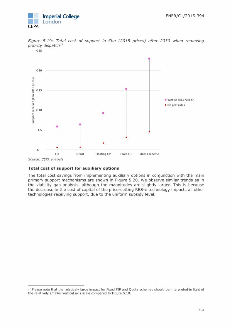
ENER/C1/2015-394

124

Figure 5.19: Total cost of support in €bn (2015 prices) after 2030 when removing

priority dispatch77


Total cost of support for auxiliary options

The total cost savings from implementing auxiliary options in conjunction with the main

primary support mechanisms are shown in Figure 5.20. We observe similar trends as in

the viability gap analysis, although the magnitudes are slightly larger. This is because

the decrease in the cost of capital of the price-setting RES-e technology impacts all other

technologies receiving support, due to the uniform subsidy level.

77 Please note that the relatively large impact for Fixed FIP and Quota schemes should be interpreted in light of the relatively smaller vertical axis scale compared to Figure 5.18.

€ -

€ 5

€ 10

€ 15

€ 20

€ 25


Sup

po

rt r

ece

ive

d (€

bn

20

15

pri

ces)

WeSIM RES27/EE27

No pref rules

ENER/C1/2015-394

125

Figure 5.20: Savings from development finance and carbon contracting on primary cost

of support between 2020 and 2050 in €bn (2015 prices)


5.2.3 Results: EU-wide and regional implementation

In addition to national policy options, we also assessed the funding gap and total cost of

support for a subset of the primary options—Floating FIP, Fixed FIP and Quota scheme—

implemented at the EU level. We also considered a specific example of a partial opening

of a national Floating FIP scheme to regional cross-border competition. Our findings from

these analyses are discussed below.

EU-wide implementation

The funding gap under EU-level schemes, shown in Figure 5.21, is marginally lower than

under national schemes as discussed in Section 5.2.2. This result is driven by a decrease

in discount rates in those MS that benefit from the better credit rating of an EU

institution that is assumed to administer the scheme. For RES-e in those countries, the

lower WACC translates into a reduced individual viability gaps.78

A potentially more significant benefit of EU-wide schemes is that siting of individual RES-

e generators and the overall generation mix would be optimised across the EU, rather

than individually in each MS. However, we cannot observe this impact, because we

adopted the RES-e deployment schedules from PRIMES, which already optimises RES-e

investments at the EU level for the considered scenarios.

In practice, we envisage that an EU-wide option would need to be implemented as a

zonal auction where capacity from certain countries is capped, based on physical

interconnection limits. This could result in multiple strike prices or levels of support

across individual countries or regions resulting in a total level of support that would be

closer to that estimated for MS implementation.

78 The impact of this is slightly different to that of the development finance option discussed above, as that would be more targeted to address financial market failures.

€ -

€ 2

€ 4

€ 6

€ 8

€ 10

€ 12

€ 14

€ 16

€ 18

€ 20


Re

du

ctio

n i

n s

up

po

rt r

ece

ive

d (

€b

n 2

01

5 p

rice

s)

Development finance (high)

Development finance (low)

Carbon contracting

ENER/C1/2015-394

126

It is important to note, however, that the funding gaps of the MS and EU-wide options

are very close to each other (see Figure 5.8 and Figure 5.15), suggesting that if there

was a separate clearing price in each MS, the total cost of support would also be shown

to be very similar.

Figure 5.21: Funding gap in €bn (2015 prices) between 2020 and 2050, EU-wide

implementation


€ -

€ 50

€ 100

€ 150

€ 200

€ 250

€ 300

Floating FIP - EU Fixed FIP - EU Quota scheme - EU

Sup

po

rt r

eq

uir

ed

(€b

n 2

01

5 p

rice

s)

WeSIM RES27/EE27


WeSIM RES27/EE30

WeSIM RES30/EE30

WeSIM Ref

ENER/C1/2015-394

127

Figure 5.22: Total cost of support in €bn (2015 prices) between 2020 and 2050, EU-wide

implementation


Regional implementation

The current Renewable Energy Directive and State Aid guidelines encourage MS to

partially open their operating aid schemes to other EEA countries and Contracting Parties

of the Energy Community.79 In fact, we understand that the Commission is requiring

certain countries to partially open their schemes where they have been judged to be

discriminatory, and providing for statistical transfers for renewable generation in one

country to be attributed to another’s renewables target.80

While there is some precedent for open schemes outside the EU,81,82 it has had limited

interest from MS to date.83

79 See paragraph 122 “Guidelines on State aid for environmental protection and energy 2014-2020” (2014/C 200/01) available on the Europa.eu website here. 80 We understand this to be the case for Germany, Denmark and Estonia. See p6, Ecofys (2016). 81 The New South Wales (NSW) Greenhouse Gas Abatement Scheme (NGAS) starting in 2003 and ending in 2012 functioned similar to a Quota scheme. The scheme was applied only to electricity consumed in NSW but renewable generators outside the state could create qualifying certificates. See Centre for Energy and Environmental Markets (Apr 2005) “The NSW Greenhouse Gas Abatement Scheme: An analysis of the NGAC Registry for the 2003 Compliance Period.” 82 The majority of US states have implemented a Renewable Portfolio Standard (RPS)—an RO-type RES support scheme. These schemes are generally open to out-of-state RES generation, although several states have introduced in-state requirements. Such requirements have raised concerns with respect to the Commerce Clause of the United States Constitution, which prohibits states from favouring local industry to the disadvantage of out-of-state competitors. Requirements that a project be located in a state or region to qualify for the RPS are considered to be discriminatory because they treat in-state and out-of-state projects differently solely for geographic reasons. For more information see Clean Energy States Alliance (2011). 83 Sweden operates a joint RO scheme with non EU-member Norway. We understand that Germany, Netherlands and the UK previously announced that they might partially open schemes but that ambition has

€ -

€ 200

€ 400

€ 600

€ 800

€ 1,000

€ 1,200

Floating FIP (monthly) -EU

Fixed FIP - EU Quota scheme - EU

Sup

po

rt r

ece

ive

d (€

bn

20

15

pri

ces)

WeSIM RES27/EE27


WeSIM RES27/EE30

WeSIM RES30/EE30

WeSIM Ref

http://eur-lex.europa.eu/legal-content/EN/TXT/HTML/?uri=CELEX:52014XC0628(01)&from=EN

http://ec.europa.eu/competition/consultations/2012_state_aid_environment/recs_3_en.pdf

ENER/C1/2015-394

128

In theory, the benefits of regional cooperation come through optimising the generation

mix across a broader geographic area, as opposed to within each county individually.

This would lead to a different mix of technologies across countries and, for Europe as a

whole, should lead to a lower cost mix of RES-e overall. However, we are unable to

capture this theoretical benefit fully because RES-e deployment was an input to the

modelling, adapted from PRIMES (and therefore not re-optimised across Europe).

However, we can observe some benefits, both on in terms of potential impacts on the

funding gap and cost of support, by simulating the partial opening of a national scheme.

In essence, we estimate how support costs would change if a country were able to shift

some of their generation into a neighbouring country with lower viability gaps (i.e.,

where RES-e is more viable).

We have identified an option for how a partially-open Floating FIP scheme could be

structured. Overall, we find that the partial opening of Floating FIP may be an interesting

option for the MS to pursue, despite its inferior performance in some respects, compared

to a fully-joint scheme. Partial opening of national schemes could also be a means of

transitioning to more efficient joint support schemes in the longer term.

Partially-open Floating FIP

We chose the partial opening of a Floating FIP because of its relatively good

performance. The assumed scheme is “open” in the sense that it allows generators in

one country to receive operating aid from the scheme of another country. We assume

that such a process is backed by arrangements for the “off-taker” country offering the

scheme to receive a statistical transfer of renewable generation from the “host” country

where the physical capacity will be located.

We envisage this scheme as being technology-neutral, excluding any technologies

deemed to be viable without support. This is consistent with our assessment of operating

aid schemes in this study.

The scheme we consider is only “partially” open in terms of there being a limit on the

total MWh tendered that generators in the host countries can access. For simplicity, we

consider a cap defined as ten percent of the total physical interconnection capacity

between the off-taker and the host country.

Auction design and incentives

Assuming they do not have access to another partially open scheme themselves,

opening a scheme should retain the same incentives for RES-e generators in the off-

taking country as under a closed scheme. The impact is more profound for the investors

in the host country as they will now face the choice between two support schemes. To

consider the implications of this, we assume that the host country provides a closed

Floating FIP scheme, and that the auctions to determine strike prices in each country are

held simultaneously. Other aspects of the allocation mechanisms would also be

harmonised, so that potential bidders in the host country can decide whether it is more

advantageous for them to participate in their domestic or the cross-border scheme.

In a competitive auction, each bidder would bid their own €/MWh revenue requirement.

To preserve this incentive, it is necessary to establish a reference price for the Floating

FIP that is based on the market where the RES-e generator is located. Thus, the RES-e

generator located in the off-taker country would be settled against the off-taker

country’s market price, and the RES-e generator located in the host country would be

settled against its domestic market price (the two reference prices would be the same if

not yet been implemented. See Klessmann (Nov 2014) “Renewable electricity support schemes in Europe: Trends and perspectives” available on the Axpo website here.

http://www.axpo.com/axpo/no/en/products/feedback_nordic_forum_2014/confirmation/jcr:content/contentPar/downloadtable/linksTop/corinna_klessmann/file.res/Corinna%20Klessmann.pdf

ENER/C1/2015-394

129

the markets are coupled and there is sufficient transmission capacity to allow the

markets to clear at a uniform price).

Under a partially-open Floating FIP, both domestic and cross-border RES-e compete on

an equal basis for support by bidding a €/MWh strike price for the Floating FIP. The

marginal bid required to meet the target will set the strike price for all cleared bids. As

long as the limit on RES-e imports is not reached, both domestic and cross-border RES-e

cleared in the auction will receive the same strike price. If the RES-e import limit is

binding, then the auction-clearing strike prices will separate: RES-e in the off-taker

country will receive a higher strike price than RES-e in the host country.

The tendering process for a partially open Floating FIP would be undertaken as a zonal

auction. This might result in multiple clearing strike prices for each location. There are

several practical examples of such locational auctions, including the locational capacity

auctions in the PJM market in the US, as well as the Zonal Auction used for demand side

response across ten electrical zones in Ontario, Canada. An illustration of this type of

auction is provided below in Figure 5.23.

Figure 5.23: Illustration of Ontario demand side response zonal auction

Source: IESO84

As shown in the figure above, capacity limits (determined based on locational limitations

or regional needs from planning studies) result in multiple clearing prices. We consider a

similar auction type could be used for a partially-open Floating FIP, where the clearing

bid would be the highest accepted bid from each zone. We also note that the

contemplated locational RES-e support auction would be similar in principle to the

market coupling process implemented in EU electricity markets.

To enhance public acceptance in the off-taker country of providing support to cross-

border RES, cleared cross-border RES-e bids could be paired with Financial Transmission

Rights (FTRs). This would guarantee to the consumers in the off-taker country that they

would have access to the RES-e generation they supported at the same price as in their

domestic market.

84 Section 5.2, IESO (Sep 2015).

ENER/C1/2015-394

130

Simulated auction case study: with tidal range

Using results from the WeSIM RES27/EE27 scenario, we simulate the impact of opening

of a Floating FIP scheme to a single neighbouring country.85 We consider the

hypothetical case of France opening its Floating FIP to Germany for projects completing

construction in 2025.86 This case was selected on the basis of outputs from our viability

model that indicated such a case might offer an efficiency improvement, compared to

running two parallel closed schemes.

Table 5.2 below presents the results of simulated auctions with closed, national-only

schemes in France and Germany in 2025 under the WeSIM RES27/EE27 scenario.

Table 5.2: Simulated Floating FIP auction bids for new generation in 2025

Incremental

capacity (MW)

Incremental

annual

generation

(GWh)

Require

support?

Estimated 15-

year strike

price (€/MWh,

2015 prices)

France (closed)

Tidal range 68 169 Yes *254

Offshore wind 129 404 Yes 131

Solar PV 1 2 No -

Onshore wind 11 27 No -

Germany (closed)

Offshore wind 2,476 8,490 Yes *107

Solar PV 2,875 2,168 Yes 88

Onshore wind 782 1,429 No -

Hydro ROR 7 33 No -

Source: CEPA calculations * Auction-clearing price

In the case shown above, France is forecast to see new solar PV and onshore wind

capacity come online in 2025, but as they would be viable without support, they are

excluded from the auction. The closed French auction would therefore be held with

participation from tidal range and offshore wind only. Tidal range capacity would set the

RES-e support auction-clearing price at €254/MWh. In Germany, we see new onshore

wind and hydro ROR generation come online, but also excluded from the auction

because they would be viable based on market revenues alone. The closed German

auction, therefore, would include offshore wind and solar PV only. The auction-clearing

price would be set by offshore wind at €107/MWh.

Now suppose that some additional German RES-e capacity, that was unsuccessful in the

closed German auction, can be offered into the French auction. To determine the impact

on the French auction, we must establish:

whether the ten percent capacity limit would be binding;

what additional German RES-e would participate; and

what strike price the German RES-e might offer.

85 Please note that for simplicity, small quantities of non-viable biomass (10MW for France and 1MW for Germany) have been excluded from this simulation. 86 Given the lead time on projects, we assume that the auction itself would be held multiple years ahead of 2025, potentially as early as 2020.

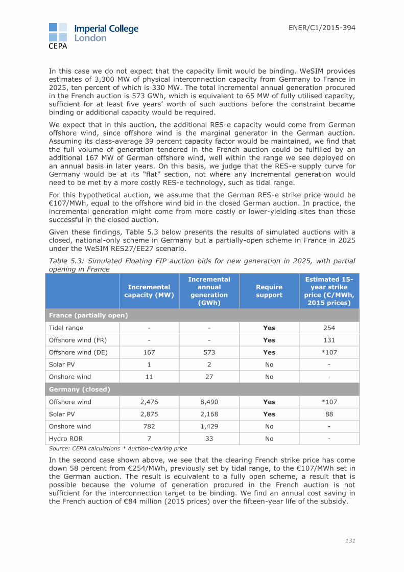
ENER/C1/2015-394

131

In this case we do not expect that the capacity limit would be binding. WeSIM provides

estimates of 3,300 MW of physical interconnection capacity from Germany to France in

2025, ten percent of which is 330 MW. The total incremental annual generation procured

in the French auction is 573 GWh, which is equivalent to 65 MW of fully utilised capacity,

sufficient for at least five years’ worth of such auctions before the constraint became

binding or additional capacity would be required.

We expect that in this auction, the additional RES-e capacity would come from German

offshore wind, since offshore wind is the marginal generator in the German auction.

Assuming its class-average 39 percent capacity factor would be maintained, we find that

the full volume of generation tendered in the French auction could be fulfilled by an

additional 167 MW of German offshore wind, well within the range we see deployed on

an annual basis in later years. On this basis, we judge that the RES-e supply curve for

Germany would be at its “flat” section, not where any incremental generation would

need to be met by a more costly RES-e technology, such as tidal range.

For this hypothetical auction, we assume that the German RES-e strike price would be

€107/MWh, equal to the offshore wind bid in the closed German auction. In practice, the

incremental generation might come from more costly or lower-yielding sites than those

successful in the closed auction.

Given these findings, Table 5.3 below presents the results of simulated auctions with a

closed, national-only scheme in Germany but a partially-open scheme in France in 2025

under the WeSIM RES27/EE27 scenario.

Table 5.3: Simulated Floating FIP auction bids for new generation in 2025, with partial

opening in France

Incremental

capacity (MW)

Incremental

annual

generation

(GWh)

Require

support

Estimated 15-

year strike

price (€/MWh,

2015 prices)

France (partially open)

Tidal range - - Yes 254

Offshore wind (FR) - - Yes 131

Offshore wind (DE) 167 573 Yes *107

Solar PV 1 2 No -


Germany (closed)


Solar PV 2,875 2,168 Yes 88


Hydro ROR 7 33 No -


In the second case shown above, we see that the clearing French strike price has come

down 58 percent from €254/MWh, previously set by tidal range, to the €107/MWh set in

the German auction. The result is equivalent to a fully open scheme, a result that is

possible because the volume of generation procured in the French auction is not

sufficient for the interconnection target to be binding. We find an annual cost saving in

the French auction of €84 million (2015 prices) over the fifteen-year life of the subsidy.

ENER/C1/2015-394

132

We also tested the impact on other system costs in 2025 that would result from the

increase in German offshore wind, and decrease in French offshore/tidal capacity that

occurs from the auction. We found fairly small savings in overall system costs of circa

€2m (compared to total system costs of over €90 billion). This impact is small, even

when comparing to the cost savings for in the French auction. This may be partly due to

the fact that the generation mix, provided by PRIMES, is already optimised on an EU-

wide basis, and so additional system cost savings are limited.

In the example above, we considered a case where the French scheme was partially

open in theory, but in practice it behaved as if it were fully open. To consider a scenario

of where participation might be more restricted, we impose an additional constraint that

no more than ten percent of total generation tendered could come from a host country.

The simulated auction results are provided in Table 5.4 below.


opening in France and a cap on participation

Incremental

capacity (MW)

Incremental annual

generation

(GWh)

Require support

Estimated 15-year strike

price (€/MWh,

2015 prices)

France (partially open)

Tidal range 45 112 Yes *254

Offshore wind (FR) 129 404 Yes 131

Offshore wind (DE) 17 57 Yes *107

Solar PV 1 2 No -


Germany (closed)


Solar PV 2,875 2,168 Yes 88


Hydro ROR 7 33 No -


The results from this third auction show that the French auction-clearing strike price has

not changed, remaining at €254/MWh, as tidal range is not displaced by German

offshore wind, because the limit on cross-border participation is binding. The zonal

nature of the auction results in a separate clearing price for the German offshore wind at

€107/MWh. In this case, therefore, while there is a reduction in the annual cost of

support under the French scheme of €8 million (2015 prices) over the fifteen-year life of

the subsidy, the effective strike price is only six percent below the level in the closed

scheme, a fraction of the level achieved than the case where the generation was able to

optimise deployment across the two countries.

The results from the simulated auctions above show clear cases where regional

cooperation could unlock significant efficiency savings. However, it is important to note

that it is based on highly stylised assumptions that might result in a different outcome in

reality:

ENER/C1/2015-394

133

the RES-e supply curves considered are based on PRIMES projections, with

projected capacity being optimised on a Europe-wide basis;87

estimates do not capture the full “true” supply curves capturing transmission

costs and the full spectrum of opportunities for each technology; and

the analysis does not capture whether there is any internal congestion in

Germany that might be a barrier to participating in the French auction.

It is also important to note the link between technology viability and potential savings

from a regional scheme. The scope of this type of scheme’s impact is limited to

technologies that are not viable without support. However, under the WeSIM

RES27/EE27 scenario, we find that many types of generation will be viable without

support. Given that we expect the viability of technologies to improve over time, we

expect the benefits from partial opening to decline in most scenarios.

That said, the same arguments apply to fully-joint schemes, which may be complex to

establish. Therefore, partial opening might be a relatively easy option to implement,

while being able to deliver much of the potential efficiency gains, as long as restrictions

on participation from other MS are not set too tight.

Simulated case study: RES-e auction without tidal range

As shown in the case study above, the cost savings from partial opening of a support

scheme can be large. However, in the case above, the main benefit comes from the

ability to replace a relatively expensive technology: tidal range. When assessing the

potential benefits of partial opening of national schemes, therefore, it is worth looking at

a case where the gap between technologies is not so large.

To do this, we used the results the from the WeSIM CRA scenario, which differs

significantly from the WeSIM RES27/EE27 scenario, as RES-e deployment is the result of

the assumed continuation of national support policies and of differentiated access to

capital conditions. This is consistent with our simulated case study auction where the

host country would have to increase its generation to both meet its own requirements

but also participate in its neighbour’s auction. Using the results from the CRA scenario

allows us to assess the potential additional capacity that each country might have

available to it.

As previously, we simulate the impact of opening a Floating FIP scheme to a single

neighbouring country. We consider the hypothetical case of Belgium opening its Floating

FIP to Netherlands for projects completing construction in 2025.88 This case was selected

on the basis of outputs from our viability modelling that indicated such a case might

offer an efficiency improvement and given that Belgium does not have tidal range as its

price-setting technology in its national auction for that year.

Table 5.5 below presents the results of simulated auctions with closed, national-only

schemes in Belgium and Netherlands in 2025 under the CRA scenario.

87 We understand that it is for this reason that we for example see a much larger level of deployment in Germany as opposed to France in this example. 88 Please note that as with the example for the partially open scheme with France and Germany, new biomass capacity has not been included in this simulation.

ENER/C1/2015-394

134

Table 5.5: Simulated Floating FIP auction bids for new generation in 2025

Incremental

capacity (MW)

Incremental annual

generation (GWh)

Require support


price (€/MWh, 2015 prices)

Belgium (closed)

Offshore wind 86 307 Yes *103

Solar PV 260 221 Yes 81

Hydro ROR 12 37 No -


Netherlands (closed)



Onshore wind 177.6 400 No -


In the case shown above, the technologies that are not viable in 2025 in Belgium, and

therefore participate in the closed auction, are offshore wind and solar PV. Offshore wind

capacity sets the RES-e support auction-clearing price at €103/MWh. In Netherlands, the

only technologies coming online in 2025 that needs support are offshore wind and solar

PV. Onshore wind is excluded from the auction as it is viable without support. The closed

Dutch auction-clearing price is set by offshore wind at €85/MWh.

For the purpose of this simulation, we suppose that some additional Dutch RES-e

capacity that was unsuccessful in its nation auction could be offered in the Belgian

auction. To determine the impact on the Belgian auction, we must establish:

whether the ten percent assumed interconnection capacity limit would be binding;

what additional Dutch RES-e would participate; and

what strike price the Dutch RES-e might offer.

In this case, we do not expect the capacity limit to be binding. The interconnection

capacity from Netherlands to Belgium in 2025 is 2,400 MW, ten percent of which is 240

MW. The total incremental annual generation procured in the Belgian auction is equal to

528 GWh, which is equivalent to 61 MW of fully utilised capacity. Therefore, the

interconnection limit is equal to at least four years of such auctions and is therefore

assumed not to be binding.

We assume that in this partially open auction, the additional RES-e capacity would come

from Dutch offshore wind, since offshore wind is the marginal generator in the Dutch

auction and assuming a 42 percent capacity factor for Dutch offshore wind, we estimate

that 84MW of additional Dutch offshore wind could be tendered in the Belgian auction,

offsetting the full volume of Belgian offshore wind (but not the full volume of generation

tendered as solar PV in Belgian is cheaper than Dutch offshore wind). For this

hypothetical auction, therefore, we assume that the Dutch RES-e strike price would be

€85/MWh, equal to the offshore wind bid in the closed Dutch auction.

Given these findings, Table 5.6 below presents the results of simulated auctions with a

closed, national-only scheme in the Netherlands but a partially-open scheme in Belgium

in 2025 under the CRA scenario.

ENER/C1/2015-394

135


opening in Belgium

Incremental

capacity (MW)

Incremental annual

generation

(GWh)

Require support


price (€/MWh,

2015 prices)

Belgium (partially open)

Offshore wind (BE) - - Yes 103

Offshore wind (NL) 84 307 Yes *85

Solar PV 260 221 Yes *81








In the second case shown above, we see that the clearing Belgian strike price has come

down to €81/MWh (2015 prices), set by solar PV, compared to the previous €103/MWh

(2015 prices) clearing price set by offshore wind. Given the zonal nature of the auctions,

the clearing strike price for the Dutch offshore wind is separate, set at €85/MWh in the

closed Dutch auction. In this example, Belgian offshore wind is completely offset by the

Dutch offshore wind, a result that is equivalent to a fully open scheme, possible because

the volume of generation procured in the Belgian auction is not sufficient for the

interconnection target to be binding. We find an annual cost saving in the Belgian

auction of €10m (in 2015 prices) over the fifteen-year life of subsidy, representing in

relative terms, a saving of 19 percent of annual support costs.

In the example above, we considered a case where the Belgian scheme was partially

open in theory, but in practice it behaved as if it were fully open. To consider a scenario

of where participation might be more restricted, we impose an additional constraint that

no more than ten percent of total generation tendered could come from a host country.

The simulated auction results are provided in Table 5.7 below.

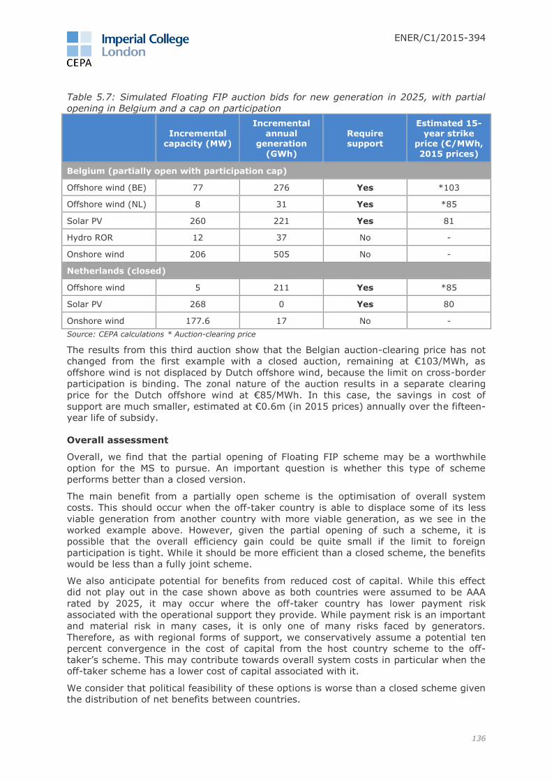
ENER/C1/2015-394

136


opening in Belgium and a cap on participation

Incremental

capacity (MW)

Incremental annual

generation

(GWh)

Require support


price (€/MWh,

2015 prices)

Belgium (partially open with participation cap)

Offshore wind (BE) 77 276 Yes *103

Offshore wind (NL) 8 31 Yes *85









The results from this third auction show that the Belgian auction-clearing price has not

changed from the first example with a closed auction, remaining at €103/MWh, as

offshore wind is not displaced by Dutch offshore wind, because the limit on cross-border

participation is binding. The zonal nature of the auction results in a separate clearing

price for the Dutch offshore wind at €85/MWh. In this case, the savings in cost of

support are much smaller, estimated at €0.6m (in 2015 prices) annually over the fifteen-

year life of subsidy.

Overall assessment

Overall, we find that the partial opening of Floating FIP scheme may be a worthwhile

option for the MS to pursue. An important question is whether this type of scheme

performs better than a closed version.

The main benefit from a partially open scheme is the optimisation of overall system

costs. This should occur when the off-taker country is able to displace some of its less

viable generation from another country with more viable generation, as we see in the

worked example above. However, given the partial opening of such a scheme, it is

possible that the overall efficiency gain could be quite small if the limit to foreign

participation is tight. While it should be more efficient than a closed scheme, the benefits

would be less than a fully joint scheme.

We also anticipate potential for benefits from reduced cost of capital. While this effect

did not play out in the case shown above as both countries were assumed to be AAA

rated by 2025, it may occur where the off-taker country has lower payment risk

associated with the operational support they provide. While payment risk is an important

and material risk in many cases, it is only one of many risks faced by generators.

Therefore, as with regional forms of support, we conservatively assume a potential ten

percent convergence in the cost of capital from the host country scheme to the off-

taker’s scheme. This may contribute towards overall system costs in particular when the

off-taker scheme has a lower cost of capital associated with it.

We consider that political feasibility of these options is worse than a closed scheme given

the distribution of net benefits between countries.

ENER/C1/2015-394

137

Assuming that competition removes any arbitrage opportunities between the two

schemes available for RES-e generators in the host country, the clearing strike

prices would be the same, as long as the RES-e import limit is not binding in the

off-taker country. Even if the clearing strike prices separate, the host country will

face a strike price at least as high as if the off-taker country did not open their

scheme.

By contrast, in the off-taker country the strike price will be no higher than had

the scheme not been opened since bids from the host country would not be

successful. Therefore, a partially open auction will only result in a different

outcome if there is a potential host country available where the clearing strike

price is lower than in the off-taker country (i.e., a country with a lower-cost RES-

e base).

The result is a convergence in strike prices. Assuming that each country is

committed to a fixed renewable MWh target in each year, the off-taker country

will end up with a lower cost of support. The host country, however, will face a

higher cost of support. While some of the RES-e generation in the host country is

paid for by the off-taker, the increased demand for RES-e generation there

pushes them up along their supply curve, needing to fulfil their own renewables

commitments with more expensive technologies.

We assume that some degree of cooperation from the host government might need to

be secured for generators to participate in the off-taker’s support scheme on a large

scale. This is problematic given that the primary benefit of opening is for the off-taker.

However, we expect that there are potential gains from trade that could be unlocked if

governments can negotiate a mutually beneficial deal. Such a negotiation would not

necessarily need to be limited to RES-e support.

It is possible to envisage countries trading access to technology-specific support

schemes where they each have comparative advantages in each technology (e.g., the

host has better insolation but worse wind resource, therefore they open their onshore

wind scheme to the host, and the host reciprocates by opening their solar PV scheme).

This form of trade is not possible when the support scheme is technology-neutral.

However, we do not consider this to be a sufficient justification to go down the route of

technology-specific support mechanisms.

As long as the timing of auctions is aligned, we do not anticipate significant additional

complexity for investors. However, open schemes might be more complex for the MS to

implement than closed schemes. For example, market arrangements and statistical

transfers would also need to be secured, and arrangements would need to be put in

place for generators to participate from multiple countries at a time, when in practice it

is possible that there might not be any successful bids received outside the off-taker

country.

ENER/C1/2015-394

138

6 Qualitative assessment of policy options

Our quantitative assessment of policy options, discussed in the previous section, focused

only on a subset of social costs, primarily the cost of capital. In order to evaluate these

options with respect to all social cost, including those that are more difficult to quantify,

we performed a qualitative assessment against a set of pre-defined evaluation criteria.

In this section, we describe our approach to that assessment, as well as the results for

each considered policy option.

6.1 Methodology

Our methodology to the qualitative assessment consists of three main steps:

1. establishing the key objectives and principles of RES-e support options, including

implications for the design of the options;

2. establishing specific evaluation criteria, based on the objectives and principles

identified in the first step; and

3. assessing each policy option against the pre-defined set of criteria to ensure

consistency.

As shown in Figure 6.1, we identified five main objectives and principles:

1. the ability to attract the required RES-e investments;

2. the ability to meet the RES-e targets at least cost;

3. compatibility with EU energy policy;

4. simplicity; and

5. provision of support only to those RES-e technologies that would not be viable

based on market revenues alone.

Figure 6.1: Main objectives and principles and their implications for policy option design

Each objective and principle has implications for the design of the policy options. The

first objective—the ability to attract the required RES-e investments—implies that the

policy option must be credible, such that investors can be reasonably confident that, with

the support, their investments will be fully remunerated. It also implies that the MS

ENER/C1/2015-394

139

governments or the EU are able to make a credible commitment to meeting the RES-e

targets by providing the required amount of support. Thus, the investors do not face a

significant risk of reduced support levels or retroactive changes in the future, nor that an

MS reneges on its commitment altogether.

We consider that the best way to achieve the second objective—meeting targets at least

cost—is through technology-neutral schemes and competitive allocations mechanisms. In

a technology-neutral scheme the various RES-e technologies are allowed to compete for

support side-by-side on a level playing field. This means that each MWh generated by a

RES-e technology is treated exactly the same as a MWh generated by any other RES-e

technology. When coupled with a competitive allocation mechanism that allocates

support to the most cost-competitive technologies, such schemes are the most likely to

minimise overall social costs89 of meeting the RES-e targets.90 They also have the added

benefit of reducing reliance on administrative parameters (e.g., setting different levels of

support for different types of RES), which often turn out to be erroneous and may result

in overcompensation.

The third objective is to ensure that the policy option is compatible with EU energy policy

up to 2030 and beyond. The current Energy and Environment State Aid Guidelines,

applicable up to 2020, significantly limit the application of some potential policy

options—rendering some of them complements, rather than alternatives of each other.91

For example, the Guidelines stipulate that operating aid recipients must be subject to

standard balancing responsibilities, unless they operate in a region without a liquid

intraday market, or if the RES-e installation is small (3 MW for wind, 500 kW for other

RES) or a demonstration project.92 In addition, RES-e support must generally be

allocated via competitive auctions or other bidding process that are open to all

technologies, except in those cases when technology-specific tenders can be justified, or

when the installations are small. The Guidelines justify technology-specific tenders on

the basis of any of the following reasons:

1. longer-term potential of a new, innovative technology;

2. the need to achieve diversification;

3. network constraints; or

4. grid stability and system integration costs.93

Exemptions are allowed for installations of a certain size, for which it cannot be

presumed that a bidding process would be appropriate or for installations at a

demonstration phase.94 The Guidelines state that RES-e aid schemes will be authorised

for a maximum period of ten years95, but they do not put a limit on the duration of

support that is received under those schemes.

The Guidelines also place some restrictions on the types of RES-e support schemes that

can be applied. They foresee the gradual replacement of FIT schemes with feed-in

premiums, which expose RES-e generators to market signals. Specifically, FIT should

only be used to support new, small-scale installations (3 MW for wind, 500 kW for other

89 We take a broad view to include all system costs, including deadweight costs arising from incentives created by policy options that induce inefficient market behaviour (e.g., distortions to bidding behaviour that result in inefficient dispatch and/or market prices). 90 Note that a non-technology-neutral scheme could potentially result in a lower total cost of support if the government had sufficient information about technology costs and if it were able to effectively price discriminate between technologies. We do not believe that in practice this is possible. 91 EC (2014a) 92 EC (2014a), section 3.3.2.1. (124)(b) 93 Ibid, section 3.3.1.(110) 94 Ibid, section 3.3.1. (109) 95 Ibid, section 3.3.1. (121)

ENER/C1/2015-394

140

RES) or a demonstration project.96 RO (Quota) schemes must not result, in the

aggregate, in overcompensation over time and across technologies, and they must not

dissuade RES-e from becoming more competitive.97 Lastly, all investment aid, where the

support exceeds €15 million, is individually notifiable.98 The MS providing such aid must

justify the need for such aid, for example, by demonstrating that a market failure exists.

When developing and assessing the policy options, we assumed that the principles laid

down in the Guidelines would remain in effect after 2020.

Simplicity of RES-e policy options refers to both the requirement that the support

scheme be relatively simple and easy to understand from the perspective of RES-e

investors, and also that they are implementable and practical. Relatively simple schemes

are not always the ones that are most optimal from a theoretical perspective. Therefore,

there are inherent trade-offs between this and the other objectives.

Lastly, to avoid overcompensation, it is desirable to extend financial support only to

those RES-e technologies that are not viable on market revenues alone. Achieving this

objective requires defining clear eligibility rules, as well as a methodology to periodically

assess the viability of RES-e technologies.

Taking into account these objectives, we established specific evaluation criteria,

summarised by category, in Figure 6.2.

Figure 6.2: Criteria used for qualitative assessment99

The revenue and cost criteria are directly related to the objective to minimise social

costs. Thus, the primary criterion in this category is overall social cost. Other costs and

risks include uncertainty of revenue streams, cost of capital, windfall profits, and

deadweight costs.

Past experience with RES-e support suggests that support schemes that are not robust

to changing market conditions are not likely to be sustainable in the long term, and are

likely to lead to abrupt changes and low confidence in the policy. Thus, the ideal policy

option minimises the risk of future re-design and the risk of errors in setting key

parameters.

We consider the risk of unintended consequences is the key regulatory risk. This includes

a wide range of risk factors, including imperfections in overall energy market design that

may have negative implications on RES-e. Other risks include subsidy risk (i.e., that the

RES-e fails to receive the support that it was promised), policy uncertainty and

credibility, and complexity.

96 Ibid, section 3.3.2.1.(124) 97 Ibid, section 3.3.2.4 (136) 98 Ibid 3.3.2.4.(136) 99 We consider the criteria shown in bold font the most important.

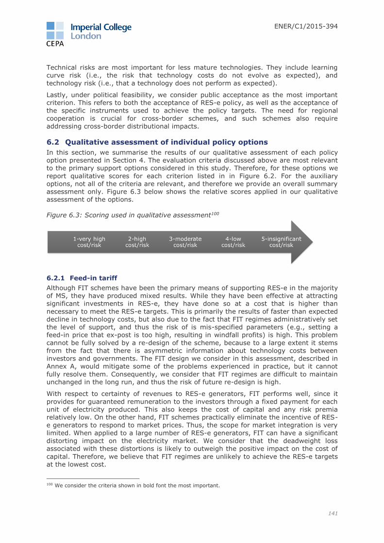
ENER/C1/2015-394

141

Technical risks are most important for less mature technologies. They include learning

curve risk (i.e., the risk that technology costs do not evolve as expected), and

technology risk (i.e., that a technology does not perform as expected).

Lastly, under political feasibility, we consider public acceptance as the most important

criterion. This refers to both the acceptance of RES-e policy, as well as the acceptance of

the specific instruments used to achieve the policy targets. The need for regional

cooperation is crucial for cross-border schemes, and such schemes also require

addressing cross-border distributional impacts.

6.2 Qualitative assessment of individual policy options

In this section, we summarise the results of our qualitative assessment of each policy

option presented in Section 4. The evaluation criteria discussed above are most relevant

to the primary support options considered in this study. Therefore, for these options we

report qualitative scores for each criterion listed in in Figure 6.2. For the auxiliary

options, not all of the criteria are relevant, and therefore we provide an overall summary

assessment only. Figure 6.3 below shows the relative scores applied in our qualitative

assessment of the options.

Figure 6.3: Scoring used in qualitative assessment100

6.2.1 Feed-in tariff

Although FIT schemes have been the primary means of supporting RES-e in the majority

of MS, they have produced mixed results. While they have been effective at attracting

significant investments in RES-e, they have done so at a cost that is higher than

necessary to meet the RES-e targets. This is primarily the results of faster than expected

decline in technology costs, but also due to the fact that FIT regimes administratively set

the level of support, and thus the risk of is mis-specified parameters (e.g., setting a

feed-in price that ex-post is too high, resulting in windfall profits) is high. This problem

cannot be fully solved by a re-design of the scheme, because to a large extent it stems

from the fact that there is asymmetric information about technology costs between

investors and governments. The FIT design we consider in this assessment, described in

Annex A, would mitigate some of the problems experienced in practice, but it cannot

fully resolve them. Consequently, we consider that FIT regimes are difficult to maintain

unchanged in the long run, and thus the risk of future re-design is high.

With respect to certainty of revenues to RES-e generators, FIT performs well, since it

provides for guaranteed remuneration to the investors through a fixed payment for each

unit of electricity produced. This also keeps the cost of capital and any risk premia

relatively low. On the other hand, FIT schemes practically eliminate the incentive of RES-

e generators to respond to market prices. Thus, the scope for market integration is very

limited. When applied to a large number of RES-e generators, FIT can have a significant

distorting impact on the electricity market. We consider that the deadweight loss

associated with these distortions is likely to outweigh the positive impact on the cost of

capital. Therefore, we believe that FIT regimes are unlikely to achieve the RES-e targets

at the lowest cost.

100 We consider the criteria shown in bold font the most important.

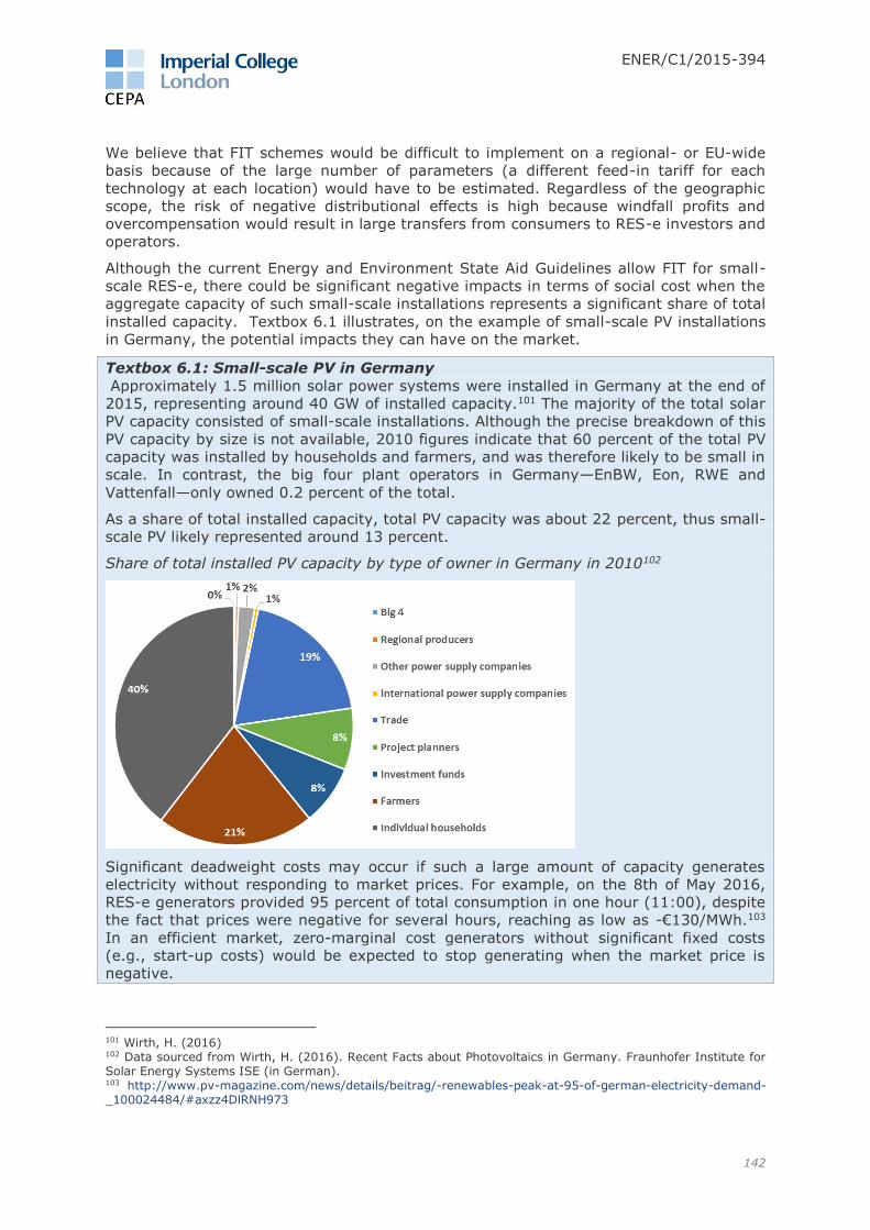
ENER/C1/2015-394

142

We believe that FIT schemes would be difficult to implement on a regional- or EU-wide

basis because of the large number of parameters (a different feed-in tariff for each

technology at each location) would have to be estimated. Regardless of the geographic

scope, the risk of negative distributional effects is high because windfall profits and

overcompensation would result in large transfers from consumers to RES-e investors and

operators.

Although the current Energy and Environment State Aid Guidelines allow FIT for small-

scale RES-e, there could be significant negative impacts in terms of social cost when the

aggregate capacity of such small-scale installations represents a significant share of total

installed capacity. Textbox 6.1 illustrates, on the example of small-scale PV installations

in Germany, the potential impacts they can have on the market.

Textbox 6.1: Small-scale PV in Germany

Approximately 1.5 million solar power systems were installed in Germany at the end of

2015, representing around 40 GW of installed capacity.101 The majority of the total solar

PV capacity consisted of small-scale installations. Although the precise breakdown of this

PV capacity by size is not available, 2010 figures indicate that 60 percent of the total PV

capacity was installed by households and farmers, and was therefore likely to be small in

scale. In contrast, the big four plant operators in Germany—EnBW, Eon, RWE and

Vattenfall—only owned 0.2 percent of the total.

As a share of total installed capacity, total PV capacity was about 22 percent, thus small-

scale PV likely represented around 13 percent.

Share of total installed PV capacity by type of owner in Germany in 2010102

Significant deadweight costs may occur if such a large amount of capacity generates

electricity without responding to market prices. For example, on the 8th of May 2016,

RES-e generators provided 95 percent of total consumption in one hour (11:00), despite

the fact that prices were negative for several hours, reaching as low as -€130/MWh.103

In an efficient market, zero-marginal cost generators without significant fixed costs

(e.g., start-up costs) would be expected to stop generating when the market price is

negative.

101 Wirth, H. (2016) 102 Data sourced from Wirth, H. (2016). Recent Facts about Photovoltaics in Germany. Fraunhofer Institute for Solar Energy Systems ISE (in German). 103 http://www.pv-magazine.com/news/details/beitrag/-renewables-peak-at-95-of-german-electricity-demand-_100024484/#axzz4DlRNH973

http://www.pv-magazine.com/news/details/beitrag/-renewables-peak-at-95-of-german-electricity-demand-_100024484/#axzz4DlRNH973


ENER/C1/2015-394

143

Hourly generation in Germany by generator type on 8 May 2016

Source: Agora Energiewende website, https://www.agora-energiewende.de

In some case, FIT could be justified in some cases on efficiency grounds, including:

Small-scale RES-e that is cost-competitive vis-à-vis large-scale RES-e, but due to

its scale and transaction costs involved, may not be able to participate in the

wholesale markets. This makes other policy options (e.g., feed-in premium

schemes) that provide support only to fill in the viability gap, and expect RES-e to

earn the remaining revenues from the market, infeasible. The justification should

also account for the possibility that aggregators could enable market access to

small RES-e, and explain why such aggregation is not possible (e.g., due to some

barriers). The FIT should be designed in such a manner that small-scale RES-e

generation would not be fed into the system when the market price is below their

marginal cost (i.e., in the case of solar PV, when the market price is negative).

Certain RES-e currently have high costs which means they are not competitive in

a technology-neutral RES-e support mechanism, but they could benefit from

significant learning and cost reductions if more installations were built. Hence, it

may be appropriate to provide support in the short-term via a FIT if this reduces

the overall cost of support in the long term.

Our overall assessment of FIT against the evaluation criteria is summarised below.

Criteria group Criterion Cost/Risk

Revenues and costs

Uncertainty of revenue streams Very low

Cost of capital and risk premiums Very low

Risk of windfall profits Very high

Risk of deadweight costs Very high

Overall system costs High

Flexibility and robustness Risk of mis-specified parameters Very high

Risk of future need for re-design Very high

Regulatory

Subsidy risk Very low

Policy uncertainty /credibility risk High

Complexity Very low

Risk of unintended consequences Very high

https://www.agora-energiewende.de/

ENER/C1/2015-394

144


Technical Learning curve / technology cost risk High

Technology risk High

Political feasibility Need for regional cooperation N/A

Negative distributional impacts High

6.2.2 Floating feed-in premium (Floating FIP)

In a Floating FIP scheme, RES-e producers sell their electricity directly into the wholesale

market, for which they receive the electricity market price and a premium that varies

with the market prices. The premium is calculated as the difference between the RMP

(€/MWh) and the strike price (€/MWh). Compared to FIT, investment risks are higher,

since RES-e has to be marketed. On the other hand, RES-e investors are exposed to less

wholesale market prices risk than under a Fixed FIP scheme.

An important design decision is on the timeframe of the RMP, which could range from an

hourly fixed RMP to a yearly fixed RMP. On one hand, an hourly fixed RMP minimises the

risk for RES-e producers, as it essentially guarantees that the strike price will be paid in

every hour. At the same time, any incentive for market integration would be removed,

since the RES-e generator would have little incentive to respond to the market price.

Conversely, a monthly or longer fixed RMP will lead to greater market integration, as

producers will be incentivised to optimise their output across months/seasons, but it will

also increase the risk for RES-e producers. Thus, setting the reference period involves a

trade-off between achieving higher levels of market integration and transferring a

bearable share of risk to RES-e producers. Our analysis suggests that the greatest

benefits are gained from moving from an hourly RMP to a daily RMP. Thus, we

recommend setting an RMP that is set on a daily or longer basis.

Once the timeframe of the RMP has been chosen a decision also has to be made on

whether the RMP is set ex-ante or ex-post. While an ex-ante RMP, based on forward

prices, provides predictability to producers, it also reduces the incentive to react to

short-term price signals. In contrast, ex-post RMP incentivises producers to optimise the

generation profile, to the extent they are dispatchable.

Overall, the Floating FIP guarantees the long-term revenue of RES-e producers by

removing the wholesale price risk associated with other options, such as Fixed FIP.

Therefore, in terms of certainty of revenues and cost of capital, this options ranks high.

Other advantages associated with the Floating FIP include the alignment of risk level

between RES-e and conventional producers. Through a Floating FIP, RES-e producers

gain skills surrounding market participation, which will be valuable during the transition

to no support. On the other hand, the design of the Floating FIP means that the actual

premium paid depends on the development of the electricity market price. Consequently,

the public bears higher risks in terms of policy costs. Moreover, depending on the RMP

timeframe, the incentive of producers to adjust output to market signals may still be

distorted. For these reasons, we consider that the risk of windfall profits, deadweight

loss and unnecessarily high system costs is moderate.

In terms of flexibility and robustness, we consider a Floating FIP to be a moderate risk

because it locks in a strike price for a relatively long period, leaving room for adjusting

the support mechanism only for RES-e procured in the future. In terms of regulatory

risk, the Floating FIP is low-to-medium risk on most aspects. Subsidy and policy is risk is

relatively low because if a Floating FIP is implemented as private CfD, since the RES-e

investor has a legal recourse in case of non-performance. The mechanism is also

relatively simple. The risk of unintended consequences is relatively moderate. This is

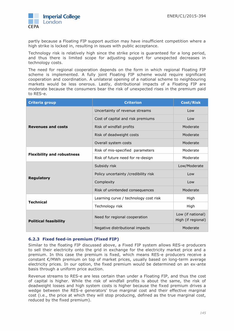
ENER/C1/2015-394

145

partly because a Floating FIP support auction may have insufficient competition where a

high strike is locked in, resulting in issues with public acceptance.

Technology risk is relatively high since the strike price is guaranteed for a long period,

and thus there is limited scope for adjusting support for unexpected decreases in

technology costs.

The need for regional cooperation depends on the form in which regional Floating FIP

scheme is implemented. A fully joint Floating FIP scheme would require significant

cooperation and coordination. A unilateral opening of a national scheme to neighbouring

markets would be less onerous. Lastly, distributional impacts of a Floating FIP are

moderate because the consumers bear the risk of unexpected rises in the premium paid

to RES-e.


Revenues and costs

Uncertainty of revenue streams Low

Cost of capital and risk premiums Low

Risk of windfall profits Moderate

Risk of deadweight costs Moderate

Overall system costs Moderate

Flexibility and robustness Risk of mis-specified parameters Moderate

Risk of future need for re-design Moderate

Regulatory

Subsidy risk Low/Moderate

Policy uncertainty /credibility risk Low

Complexity Low

Risk of unintended consequences Moderate



Political feasibility Need for regional cooperation

Low (if national)

High (if regional)

Negative distributional impacts Moderate

6.2.3 Fixed feed-in premium (Fixed FIP)

Similar to the floating FIP discussed above, a Fixed FIP system allows RES-e producers

to sell their electricity onto the grid in exchange for the electricity market price and a

premium. In this case the premium is fixed, which means RES-e producers receive a

constant €/MWh premium on top of market prices, usually based on long-term average

electricity prices. In our option, the fixed premium would be determined on an ex-ante

basis through a uniform price auction.

Revenue streams to RES-e are less certain than under a Floating FIP, and thus the cost

of capital is higher. While the risk of windfall profits is about the same, the risk of

deadweight losses and high system costs is higher because the fixed premium drives a

wedge between the RES-e generators' true marginal cost and their effective marginal

cost (i.e., the price at which they will stop producing, defined as the true marginal cost,

reduced by the fixed premium).

ENER/C1/2015-394

146

We consider that in terms of flexibility and robustness, Fixed FIP schemes rank the same

as Floating FIP (i.e., moderate risk/cost).

The subsidy risk is relatively low, since the premium is set ex ante, and it is not subject

to any adjustments ex-post. In terms of policy credibility and complexity, we score this

option lower than the Floating FIP because support is determined not in terms of total

price needed for remuneration of RES-e investments, but rather relative to the future

market price, which is inherently uncertain. For the same reason, technical risks are

moderate.

Lastly, on political feasibility criteria, this option scores the same as a Floating FIP.


Revenues and costs

Uncertainty of revenue streams Moderate

Cost of capital and risk premiums Moderate


Risk of deadweight costs High

Overall system costs Moderate/High



Regulatory

Subsidy risk Low

Policy uncertainty /credibility risk Moderate

Complexity Moderate

Risk of unintended consequences High

Technical Learning curve / technology cost risk Moderate

Technology risk Moderate


Low (if national)

High (if regional)


6.2.4 Quota schemes

Quota schemes—also known as, RO schemes—do not guarantee a pre-determined

revenue stream to RES-e investors, and thus the uncertainty of those can be very high if

a MS does not have institutions than can credibly implement such a scheme. This,

therefore, generally results in higher cost of capital and risk premia, relative to a

Floating FIP scheme. We consider that the risk of windfall profits is about the same than

under a Floating FIP. On the other hand, if the RO mechanism accurately internalises

carbon costs not reflected in the ETS price, it is likely to lead to lower deadweight and

system costs than a Floating FIP. In terms of errors in mechanism design, we consider

the risks are roughly the same between RO and Floating FIP. Subsidy risk is very high

since the level of support is a function of RO certificate prices determined by the market,

which is likely to fluctuate. These prices will also be a function of other policy measures

that affect market fundamentals, such as ETS prices, and therefore we believe the

regulatory risks will be somewhat higher than under a Floating FIP. Technical risks are

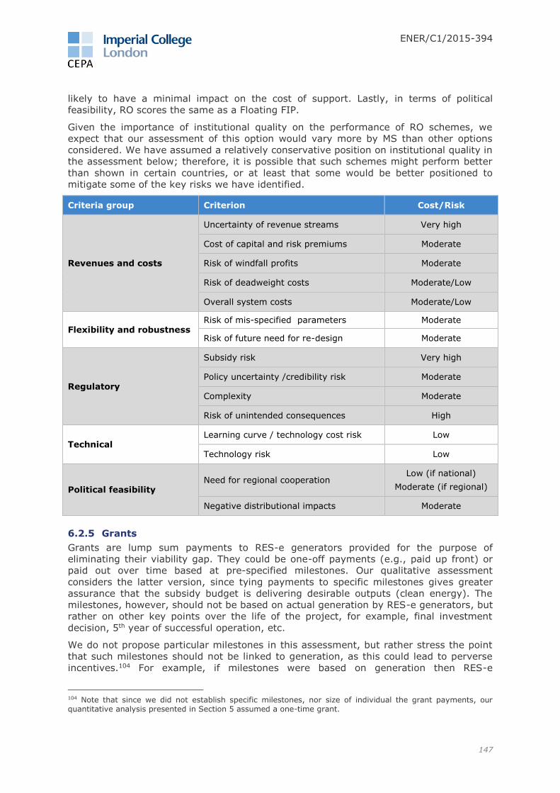
ENER/C1/2015-394

147

likely to have a minimal impact on the cost of support. Lastly, in terms of political

feasibility, RO scores the same as a Floating FIP.

Given the importance of institutional quality on the performance of RO schemes, we

expect that our assessment of this option would vary more by MS than other options

considered. We have assumed a relatively conservative position on institutional quality in

the assessment below; therefore, it is possible that such schemes might perform better

than shown in certain countries, or at least that some would be better positioned to

mitigate some of the key risks we have identified.


Revenues and costs

Uncertainty of revenue streams Very high

Cost of capital and risk premiums Moderate


Risk of deadweight costs Moderate/Low

Overall system costs Moderate/Low



Regulatory

Subsidy risk Very high

Policy uncertainty /credibility risk Moderate

Complexity Moderate

Risk of unintended consequences High

Technical Learning curve / technology cost risk Low

Technology risk Low


Low (if national)

Moderate (if regional)


6.2.5 Grants

Grants are lump sum payments to RES-e generators provided for the purpose of

eliminating their viability gap. They could be one-off payments (e.g., paid up front) or

paid out over time based at pre-specified milestones. Our qualitative assessment

considers the latter version, since tying payments to specific milestones gives greater

assurance that the subsidy budget is delivering desirable outputs (clean energy). The

milestones, however, should not be based on actual generation by RES-e generators, but

rather on other key points over the life of the project, for example, final investment

decision, 5th year of successful operation, etc.

We do not propose particular milestones in this assessment, but rather stress the point

that such milestones should not be linked to generation, as this could lead to perverse

incentives.104 For example, if milestones were based on generation then RES-e

104 Note that since we did not establish specific milestones, nor size of individual the grant payments, our quantitative analysis presented in Section 5 assumed a one-time grant.

ENER/C1/2015-394

148

generators could be incentivised to sell electricity at negative prices, if it allowed them to

unlock a grant payment. Therefore, to avoid potential perversions to bids in the energy

market we propose to delink grant payments from generation. These milestones could

nonetheless guarantee the availability of generators and the provision of clean energy.

Compared to other options, such as FITs or FIPs, grants designed in the proposed

manner could have important efficiency implications as they leave generators fully

exposed to wholesale prices and maintain the incentive for generators to respond to

prices efficiently. Uncertainty of support payments would be very low, resulting in low to

moderate risk premia. On the other hand windfall profits could be high, if despite the

safeguards, RES-e projects do not materialise. Given these risks, grants are deemed

moderate risk in terms deadweight and overall system costs.

The proposed scheme is envisaged to allocate grants through a competitive, technology-

neutral, auction (i.e., via a challenge fund). The auctions would be uniform price

auctions, open to all technologies that would not be viable without support. As with other

options, the uniform-price auction should result in an efficient overall mix of

technologies. These features should keep the risks associated with scheme flexibility and

robustness at a moderate level.

We consider that the policy and credibility risk associated with a grant scheme would be

high because large sums of support payments most likely would have to be funded from

the government budget. This could be further aggravated by potential defaults by

investors. To our knowledge, grants have only been used for RES-e support on a

relatively small scale, at least compared to the investment challenge we estimated.

Grants would also raise unique implementation challenges, for example, whether support

should be provided for MWh generated or MW of installed capacity. Given the scale of

the RES-e investment challenge in Europe, using grants on a large scale would also be

susceptible to fraud and public acceptance challenges. Grants could be used to meet

auxiliary targets (e.g., supporting innovation) if it is desired. Overall, a grant scheme

would be relatively simple, but due to the reasons cited above, subsidy risk and the risk

of unintended consequences is likely to be moderate. We consider that risks associated

with political feasibility are low to moderate.


Revenues and costs

Uncertainty of revenue streams Very low

Cost of capital and risk premiums Low/Moderate

Risk of windfall profits High

Risk of deadweight costs Moderate

Overall system costs Moderate



Regulatory

Subsidy risk Moderate

Policy uncertainty /credibility risk High

Complexity Low

Risk of unintended consequences Moderate


ENER/C1/2015-394

149




Low (if national)

Moderate (if regional)


6.2.6 Development finance

Development finance is an intervention by public sector financial institutions to mobilise

commercial capital and sometimes to reduce financing costs for RES-e projects where

affordability is an issue. This falls into two categories: market-based and concessionary

financing. Irrespective of which category, development finance comes in two forms:

Funded financial products—such as equity, mezzanine finance (such as quasi-

equity and subordinated debt) and senior debt. If provided on a concessionary

basis the return or interest rate on the product is below an equivalent market

rate.

Contingent products—such as credit guarantees and insurance/guarantees

against specific event risks, such government non-performance risks can also be

deployed. These are often unavailable from market sources: concessionary

finance involves a fee that is not fully risk-reflective.

The provision of development finance can be accompanied by provision of grant monies

that can be used to reduce transaction costs.

Development finance has potential to reduce the total cost of support to RES-e but does

come at its own cost as described above. Total cost of support could be reduced if

development finance improved the viability of the marginal RES-e generator at a given

point in time. This would occur not through reducing the volatility of their revenues but

through decreasing their cost of capital, putting greater value on future revenues to

cover upfront capital costs.

Development finance is an effective option for policy makers when it used to target

market failures in the market for financing RES-e. Market failures in the market for

financing RES-e include the impact of technology novelty on investors’ risk preferences

or balance sheet limits that make the financing of larger projects difficult, particularly

during their development and construction phases. These financing market failures have

knock-on effects in the RES-e market as they make projects facing those issues appear

more costly than they would absent those failures. Therefore, financing intervention in

these cases can remove distortions from the RES-e supply curve, potential improving

total system costs if those technologies are part of the lowest cost mix required to meet

decarbonisation objectives.

Care should be taken, however, to reduce the potential for overcompensation.

Development finance, by its nature, is administrated and therefore may not be as

responsive to market conditions as other support options, creating the potential to

provide more support than needed to address the issues it is designed to address.105 The

consequence of this may be the crowding-out of private sector capital and a distortion in

the RES-e supply curve towards these technologies.

Development finance is a relatively practical option but there are issues that need to be

managed. It is a practical option as a number of experienced administrators of

development finance (e.g., EIB, and the European Bank for Reconstruction and

105 For example, administrators may be slow to withdraw support when no longer needed.

ENER/C1/2015-394

150

Development [EBRD]) are already in existence. This demonstrates the political feasibility

of these options and willingness for international cooperation in this area. A particular

strength is the ability of development finance to facilitate technical innovation as

emerging technologies are prime beneficiaries for such finance given the financial market

failures they face around their novelty. That said, the existing level of activity in

development finance may mean that the justification for further intervention in this area

is limited or non-existent. The important factor is that it does not go so far as to create

distortions itself. If applied well, risk of unintended consequences and distributional

impacts are low. If applied poorly there may be issues around:

hostility regarding perception of double subsidising RES-e;

co-investors free-riding or overly relying on the administrator’s due diligence;

bias in favour of larger projects, more able to navigate the process to secure

development finance.

Overall, we find that development finance can be a useful option for policymakers to

pursue if used with restraint in a targeted manner.

6.2.7 Innovation-focused support

Innovation-focused support would be a technology-specific form of RES-e support.

Therefore, we consider that it could be an auxiliary support mechanisms for those RES-e

technologies that are not able to obtain support in a competitively-allocated, technology-

neutral primary support mechanism. The main rationale for implementing such

mechanisms would be that by providing support, technology learning could be

accelerated, and overall dynamic (long-term) efficiency could be improved upon. We

consider that it would be most efficient to provide such support outside the primary RES-

e support mechanism. Regarding the form of support, theoretically all options considered

for primary support could also work as innovation-focused support. Therefore, the same

advantages and disadvantages apply as discussed above for each of those options.

In Section 7, we discussed how an auxiliary innovation-focused support mechanism

could work alongside the primary support mechanism.

6.2.8 Priority dispatch

Priority dispatch is a market access rule, which places an obligation on the TSOs to

schedule and dispatch RES-e generators ahead of all other generation types. Thus,

priority dispatch artificially pushes some RES-e generators down the merit order,

displacing other lower cost conventional generators. This means that generators

receiving priority dispatch will at time sell electricity below their short-run marginal cost

(SRMC).

The purpose of priority dispatch is to provide certainty to renewable generators that they

can maximise their output, and thus increase their support payments (i.e., to reduce

volume risk). It was also seen as a tool to enable a more rapid integration of RES-e

generators into the power system. Historically, priority dispatch has been offered in

combination with other schemes, such as FIT.

In this assessment, we consider priority dispatch as a standalone policy option. For a

rational generator, priority dispatch would not be a credible form of support in-and-of

itself, since routinely selling electricity below SRMC would create financial losses. Priority

dispatch would, therefore, only be effective if combined with other forms of operational

support, which would not be desirable from an efficiency point of view.

Thus, we consider that priority dispatch would be a very ineffective and inefficient RES-e

support option. Our findings suggest that priority dispatch on its own is detrimental to

RES-e market revenues, and results in significant social (deadweight) cost.

ENER/C1/2015-394

151

6.2.9 Exemption from balancing responsibility

A unique feature of electricity is that it cannot be stored on a large scale, and therefore

ensuring the security of the electricity system requires maintaining a constant balance

between production and consumption. In EU electricity markets, market participants

have the primary responsibility for maintaining balanced schedules, while residual

balancing is carried out in real time by the TSOs. A Balancing Responsible Entity, which

represents one or more generators, suppliers and consumers, is usually in charge of

balancing contractual positions by transacting in intraday markets.

Market participants that have a disparity between their notified contractual positions and

their actual metered positions are subject to imbalance charges determined as follows:

If a participant is long, meaning they generate more than their contractual

position, they get a payment which is usually no higher than the weighted

average price for activated negative balancing energy for frequency restoration

reserves and replacement reserves; and

If a participant is short, meaning they have a deficit in relation to their

contractual positions, they are charged a penalty, which is typically no less than

the weighted average price for activated positive balancing energy for frequency

restoration reserves and replacement reserves.

Intermittent generators with limited capability to control their output face potentially

persistent imbalances, and thus balancing responsibility may expose them to significant

costs. The rationale for providing an exemption from balancing responsibility to RES-e is

that these generators are more likely to be exposed to net imbalance costs than

conventional generators. In effect, this policy option could decrease their operational

costs.

We consider this an auxiliary option, because on its own it would be insufficient to

ensure RES-e viability. Imbalance charges are not a significant source of the observed

RES-e viability gap, and they are not a major consideration when making RES-e

investment decisions.106 Since, balancing responsibility does not change the relative risk

assessment of a project, it does not have an impact on the cost of capital either.

We did not explicitly model balancing responsibility in WeSIM, because it does not have

the capability to capture all relevant trading timeframes. Thus, our conclusions are based

primarily on this qualitative assessment, supplemented with market data and secondary

sources. Given that in most MS, wind generators are already subject to balancing

responsibility under the same terms as conventional generators, it would not be

appropriate to re-introduce an exemption from balancing responsibility in those markets.

As long as liquid intraday markets exist, and imbalance prices reflect the actual cost of

balancing the system, RES-e generators should be able to minimise their exposure to

imbalance costs. An exemption from balancing responsibility would weaken the incentive

of RES-e to accurately forecast their output and could thus potentially distort the day-

ahead market. Therefore, the only justification for this policy option providing an

exemption from balancing responsibility is if the intraday and balancing markets are

illiquid and inefficient in the sense that the imbalance prices are not cost-reflective. The

objective of the policy option is therefore to compensate for a market failure rather than

making RES-e viable.

It has been reported that imbalance costs in some MS appear to be disproportionally

high.107 We examined imbalance costs faced by a typical wind generator in Austria. Our

findings are summarised in Textbox 6.2.

106 This assessment was confirmed during our June workshop with finance experts in Brussels. 107 EWEA (2015)

ENER/C1/2015-394

152

Textbox 6.2: Balancing costs for wind generators in Austria

Balancing mechanism in Austria is an example of a balancing market that displays

relatively high imbalance prices. In 2015:

Downward activation (i.e., system was long) weighted average prices were

negative: -59.7€/MWh108

Upward activation (i.e., system was short) weighted average prices were

76.1€/MWh109

These average prices are relatively high and the spread between downward and

upward activation prices is large (135€/MWh). A potential sign of inefficiency is the

fact that downward regulation prices are negative. Those negatives prices mean that

generators are systematically remunerated for reducing their production or increasing

their consumption. It could also be an indication that the system is inflexible.

In 2015, we estimated that a typical wind generator would have paid on average

15€/MWh110 in imbalance costs. These high imbalance costs can be explained by very

high imbalance prices when the system is very long. In just 27 hours during the year,

wind generators paid the equivalent of 12 percent of the annual imbalance costs. The

weighted average imbalance price during those hours when the system was very long

was negative: -265€/MWh.

The viability gap for onshore wind generators in Austria in 2015 under no support is

estimated to be 75€/MWh.111 While imbalance charges faced by wind are significant,

removing this obligation would not fill the wind generator’s viability gap. Therefore, it

is not suitable as a primary option for RES-e support. However, it could be applied as

an auxiliary option to mitigate the relatively high imbalance costs.

This policy option is easy to implement as balancing markets are usually national

markets, and therefore do not require regional cooperation. However, a national

implementation of preferential market rules could lead to distortions in the internal

market in electricity, resulting in distortions in cross-border trade. We consider that any

implementation of this option should be temporary, to be eliminated once the underlying

distortions in the balancing markets are resolved.

6.2.10 Carbon contracting

The EU ETS is a major pillar of EU climate policy and provides a platform for pricing

carbon emissions through its cap-and-trade system. Its main goals are to restrict the

total level of emissions across Europe and to incentivise participants to invest in cleaner

technology. Market participants also perceive ETS as a major source of policy risk. As

Newbery (2010) discusses, the risk associated with carbon prices is largely policy and

political, and impacts investors whose portfolios are much more focussed on renewable

electricity generation rather than those investors with a more balanced portfolio that

includes conventional generation. This is because conventional (price-setting) generators

are already hedged to some extent against carbon price volatility, as they can pass their

costs through to consumers through wholesale electricity prices.

Carbon contracting would provide eligible participants with a hedging product that

mitigates the risk of low future ETS prices caused by a failure to follow through with the

108 ENTSO-E data, 2015 109 Ibid 110 Ibid 111 CEPA analysis, 2016

ENER/C1/2015-394

153

declared carbon policy. The goal of such a product would be to address the failure of the

ETS at producing relevant carbon prices by:

Making future EU policy commitments (e.g., ETS Phase 4) more credible, by

acting as the counterparty to the contract. The EU would be at risk of paying out

large sums of money for not delivering an efficient and effective ETS.

Providing downside protection to RES-e generators: contracts would provide

insurance and increase certainty over one element of future wholesale prices.

The ability of carbon prices to drive low-carbon investments depends on the predicted

levels of ETS prices and investors' confidence that the prices will not fall below the point

at which investments become unprofitable. Carbon contracting could be set up as a CfD

on future carbon prices, either as a:

Two-sided CfD: where generators would be entitled to receive the difference

between the strike price and the spot price; or

One-sided CfD: where generators receive the difference between the strike price

and spot price only when the spot price falls below the strike price. This

essentially sets a price floor.

To achieve efficient and market driven pricing of contracts, the CfDs would be allocated

through an auction process. All parameters, apart from the price of the contract itself

(e.g., strike price, contract length, volume of contracts), would be specified

administratively.

The contract would specify a strike price, specifying a particular level of carbon price. We

envisage the contract as being purely a financial contract (i.e., not linked to generation),

with contracts specified in terms of tonnes of CO2. Therefore, investors that are bidding

for carbon contracts would need to calculate their exposure to carbon through wholesale

prices.

We consider that a one-sided CfD would likely more attractive because under a two-

sided CfD generators could be at risk of paying (if ETS prices are higher than the strike

price) even if they are not generating, since the contract is not linked to generation.

However, valuing such carbon contracts is complicated, which is likely to limit potential

interest for such a product.112

In terms of efficiency, the question is whether such a product, underwritten by the EU,

would be filling a gap in the market. Currently, one is able to purchase futures contracts

and options on ETS allowances, for example on the ICE exchange. While this does allow

market participants to hedge some volatility in prices it does not directly deal with the

root cause of the risk—policy/political risk. The benefit of carbon contracts underwritten

by the EU would be to increase the credibility of future EU policy and increase the

certainty that investors may have around the ability of the EU to reform the ETS. It may

be the case that by providing even a small number of contracts, EU ETS policies may be

seen to be more credible and reduce the perceived risk of investors who do not have a

carbon contract. However, this then raises concerns of free riding by investors. In this

case, investors who do not bid for contracts benefit from increased commitment to policy

provided by contracts bought by others.

This option would not be useful for supporting RES-e generators if they also have access

to other instruments that guarantee the wholesale price (e.g., a CfD or a FIT). However,

it may be desirable to those RES-e generators once their existing support mechanisms

come to an end, and also to generators that are not eligible for other support

mechanisms. It therefore may be useful as a means of transitioning out such a

112 This was confirmed by feedback received from the workshop held in Brussels in June.

ENER/C1/2015-394

154

mechanism and increasing the exposure of RES-e to market prices more gradually than

simply cutting off support.

Overall, this option would be a targeted measure to address one of the main sources of

policy risk. However, we consider that it is too complex, and most likely would not be

effective in practice.

6.3 Conclusions from qualitative assessment of options

Our qualitative assessment of the primary options is summarised in Figure 6.4. Overall,

we believe that Floating FIP performs best against the assessment criteria. It performs

better than FIT, Fixed FIP or RO schemes against most of the criteria. Although FIT

schemes provide more revenues certainty, and thus lower cost of capital, and they are

also relatively simple, they score much worse against other criteria, especially overall

system costs. Similarly, Fixed FIP scores better only with respect to subsidy risk, while it

ranks worse against all other criteria. RO schemes score worse, compared to FIP, with

respect to uncertainty of revenues, cost of capital, subsidy and policy uncertainty risk.

Lastly, although grants score better than FIP against some of the criteria, as discussed

earlier, given the scale of the RES-e investment challenge in Europe, using grants on a

large scale would be, politically, extremely challenging to implement. Therefore, we

believe that the primary option for RES-e support should be FIP schemes.

Nevertheless, as already discussed, policy risk is a major consideration for investors. Any

change of RES-e support policy is likely to involve significant risks, therefore the costs

and benefits of a transition to the proposed FIP should be carefully evaluated. Some

existing schemes may already deliver much the benefits are proposed FIT would;

therefore it may not be desirable to the proposed FIT, or such transition should be

managed gradually.

In addition to a primary support mechanism, auxiliary support options could also be

implemented, as long as they can be justified on ground of overall efficiency, and they

do not interfere with the primary policy options. Our recommendations are discussed in

detail in the next section.

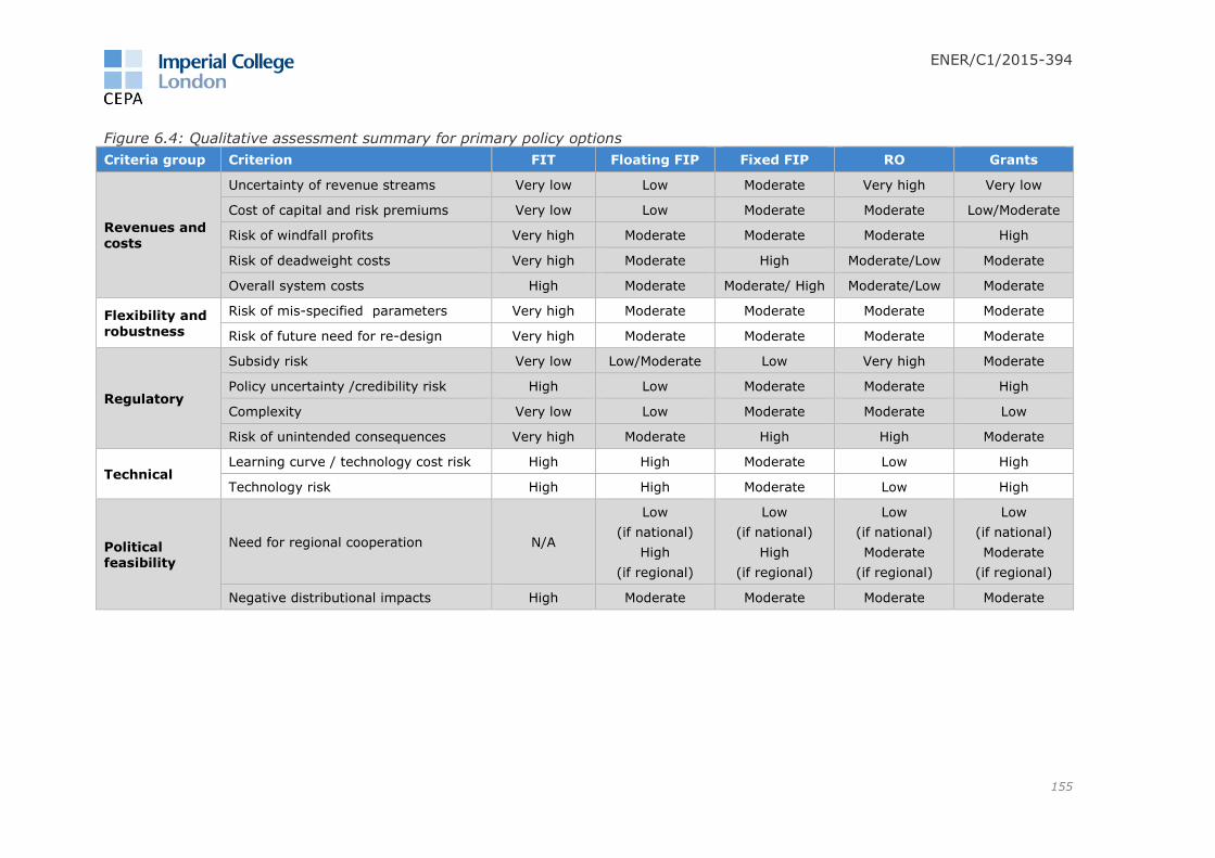
ENER/C1/2015-394

155

Figure 6.4: Qualitative assessment summary for primary policy options

Criteria group Criterion FIT Floating FIP Fixed FIP RO Grants

Revenues and

costs

Uncertainty of revenue streams Very low Low Moderate Very high Very low

Cost of capital and risk premiums Very low Low Moderate Moderate Low/Moderate

Risk of windfall profits Very high Moderate Moderate Moderate High

Risk of deadweight costs Very high Moderate High Moderate/Low Moderate

Overall system costs High Moderate Moderate/ High Moderate/Low Moderate

Flexibility and

robustness

Risk of mis-specified parameters Very high Moderate Moderate Moderate Moderate

Risk of future need for re-design Very high Moderate Moderate Moderate Moderate

Regulatory

Subsidy risk Very low Low/Moderate Low Very high Moderate

Policy uncertainty /credibility risk High Low Moderate Moderate High

Complexity Very low Low Moderate Moderate Low

Risk of unintended consequences Very high Moderate High High Moderate

Technical Learning curve / technology cost risk High High Moderate Low High

Technology risk High High Moderate Low High

Political feasibility

Need for regional cooperation N/A

Low

(if national)

High

(if regional)

Low

(if national)

High

(if regional)

Low

(if national)

Moderate

(if regional)

Low

(if national)

Moderate

(if regional)

Negative distributional impacts High Moderate Moderate Moderate Moderate

ENER/C1/2015-394

156

7 Policy recommendations for supporting RES In developing our recommendations, we considered that the primary policy objective

should be to meet future (2030) RES-e targets and 2050 decarbonisation

objectives at least cost. This should be achieved by providing financial support to

RES-e investments that would not materialise in the absence of such support, given

insufficient electricity market revenues to remunerate for such investments (i.e., a

viability gap exists).

Cost effectiveness in this context refers to social costs,113 recognising the fact that there

are inherent tensions and trade-offs between costs to investors and costs that accrue to

consumers (e.g., lowering the cost to investors may result in higher cost to consumers if

it is achieved by means that create incentives for the inefficient operation of RES-e

generators).

Since the primary policy objective should be to obtain the least-cost RES-e mix required

to meet the RES-e target, some emerging technologies—at least those that are not

required for meeting the targets—may not receive much support under our proposed

mechanism. Although, we understand that policy makers may wish to pursue other

objectives through energy/ RES-e policies—such as, resource diversity, domestic job

creation, or supporting innovation in emerging RES-e technologies. We note that

pursuing such goals—in addition to meeting the RES-e target—is likely to result in a

higher cost of meeting the primary objective. Our recommended policy option is flexible

and could allow the incorporation of additional policy objectives—assuming that the

additional costs are acceptable—but without changing the nature of the primary support

mechanism.

For example, emerging technologies, those that would likely not succeed in a

technology-neutral auction, could be excluded from the primary support mechanism, and

receive technology-specific support through an auxiliary mechanism. Based on our

current modelling, we expect that technologies including offshore wind would clear in the

primary support mechanism, while it might take some time for other technologies, such

as tidal range to fall into this category.

We have factored into our recommendations lessons learned from current and past

support mechanisms implemented in Europe and around the world. These practical

lessons have highlighted the importance of mechanisms that are not just well-designed,

but also politically feasible and implementable.

The market simulations that were performed for this study have also informed our

recommendations. Although they cover a number of future scenarios and a range of

policy options, our recommendations are not dependent on these results nor the

assumptions that underlie them. The recommended support mechanisms are robust to

changing market conditions. This is important, since the future is inherently uncertain,

and thus the support mechanism put in place should be designed to meet the primary

objective under all circumstances.

An important implication of cost efficiency of the chosen support mechanism is that RES-

e generators receiving support are well-integrated into the wholesale market and that

they respond to market signals. Thus, when assessing the policy options, we considered

potential market-distorting behaviour and their associated costs.

Taking into account the above considerations, we have concluded, based on our

qualitative and quantitative assessment, that in terms of economic efficiency, the best

113 Social costs are total costs to society.

ENER/C1/2015-394

157

way to achieve the primary objective is to provide RES-e support via a single,

primary support mechanism. This mechanism would:

Be technology-neutral—allowing direct competition among different types of

non-viable RES-e technologies for support to provide the new generation capacity

required to achieve renewables targets.114 This approach is most likely to

minimise the total cost of RES-e support by avoiding deadweight losses created in

technology-specific schemes, given that the asymmetric information problem115

regarding technology costs is likely to persist between investors and regulators.

Technology-neutral mechanisms do not rely on policymakers’ knowledge of

technology and other costs. Instead, competitive pressure in support auctions will

provide investors with an incentive to reveal these costs in their bids. This

approach would also support innovation, since offering a more cost-effective

technology would put the RES-e investors in that technology at a competitive

advantage in the support auction. RES-e investors would also have an incentive

to efficiently site their generators in locations where the overall (social) cost of

generating clean energy is the lowest.

This rests on the assumption that the charges RES-e generators face, including

transmission charges, are cost-reflective. If they were not, the investors would

still factor them into their investment decision, but the siting of the RES-e

generators may not be efficient. This does not detract from the merits of the

proposed support mechanism: the distortions occur in other parts of market

design, not RES-e support, and that is where they should be remedied. It would

not be desirable to attempt to remedy such imperfections as part of RES-e

support mechanism design.

Allocate RES-e support via competitive auctions—these auctions should be

designed in a manner that maximises potential competition. Establishing

competitive allocation mechanisms alone may not be sufficient to achieve efficient

outcomes. The level of potential competition should be continuously monitored,

and safeguards should be put in place to ensure that auction results are truly

competitive. An effective way of increasing competition is to open up RES-e

support auctions to cross-border competition. To achieve this, we make the

following recommendations:

o First-come-first-served and other non-competitive allocation

mechanisms should be phased out—several mechanisms implemented in

the past relied on non-competitive allocation mechanisms (e.g., FIT), which

likely resulted in overall costs that were higher than necessary.

o Auctions in the primary mechanism should not be designed to

distinguish between technologies beyond excluding technologies that

are viable without support (e.g., there should not be technology banding).

All cleared RES-e should receive the uniform auctioning clearing prices as

RES-e support.

o If auctions allow for cross-border participation, they should be

designed as locational auctions, whereas RES-e support is dependent on

the auction-clearing price in the market where the RES-e installation is (or will

be) located. This approach recognises that the market price of electricity may

differ between markets, and thus ensures that RES-e generators are not

overcompensated with respect to their viability gap.

114 This could, for example, mean PV and offshore wind competing in the same auction, assuming both are not viable without support. 115 RES investors have more accurate information about current and future technology costs than policymakers.

ENER/C1/2015-394

158

o Administrative procedures for determining the level of support should

be used as a last resort—a technology-neutral approach should maximise

the level of competition, especially if it covers a relatively large geographic

area. If, however, potential competition is not sufficient to achieve a

competitive outcome (e.g., concentration of bidders is high) then the reasons

for the lack of competition and potential solutions (e.g., merging a small

national scheme into a larger regional scheme) should be explored116 before

support levels are set administratively. Support levels should be set in an

administrative manner only as a fall-back option.

o We recommend assessing the level of competition before RES-e

support auctions are cleared. This would involve analysing bids before

each round of competitive allocation to check whether any bidder has the

ability and/or the incentive to distort the auction-clearing price.

The different types of policy options considered in this study do not perform equally.

Auxiliary options (preferential market rules, carbon contracting, and development

finance) would not provide sufficient support for all new RES-e required to achieve

renewables targets, and thus are not suitable as a means of primary RES-e support.

Of the investment aid options, grants in particular, could in theory achieve the RES-e

targets cost-efficiently; however large upfront costs, as well as potential defaults by

investors, could make it challenging to implement and maintain such mechanisms on a

large scale. Although this could be mitigated by issuing grant payments tied to the

achievement of specific project milestones, relying on grants as a primary mechanism

for RES-e support is largely uncharted territory in the world of RES-e support. To our

knowledge, grants have only been used for RES-e support on a relatively small scale, at

least compared to the RES-e investment challenges in Europe. Grants would also raise

unique implementation challenges, such as whether support should be provided for MWh

of energy generated or MW of installed capacity). Given the scale of the RES-e

investment challenge in Europe, using grants on a large scale might also be susceptible

to fraud and public acceptance challenges. Grants could be used to meet auxiliary

objectives, such as supporting innovation to develop immature technologies, if it is

desired.

Of the operating aid options, FIT and Fixed FIP are inferior to other options such

as Floating FIP and RO, and should therefore be phased out. FIT heavily relies on

administratively set parameters. Past implementation of FIT has resulted in

overcompensation and abrupt policy changes. Furthermore, FIT offers limited

opportunity for integrating RES-e into the wholesale markets, as generators with a FIT

are shielded from market prices. While the current Renewable Energy Directive allows for

small-scale RES-e to receive FITs, small-scale RES-e installed in large volumes can have

significant negative impacts on the wholesale market, as evidenced by the experience of

some MS. Therefore, we do not recommend allowing FIT to all small-scale RES-e

based on size alone. FIT for small-scale RES-e should only be allowed if total

capacity of small-scale RES-e does not exceed a total capacity capacity

threshold, such that small-scale RES-e in the aggregate does not have a

material impact on the wholesale market. Above this threshold, small-scale

RES-e could be supported via an auxiliary mechanism as described below.

There has been little practical experience with pure Fixed FIP schemes. We consider

them inferior to floating premium schemes. Although the level of support would be set in

competitive auctions, RES-e investors receiving fixed premia would face higher risks and

costs than under a Floating FIP given the absence of wholesale price risk protection in

116 We understand that these solutions may be politically challenging, but the potential benefits could be significant.

ENER/C1/2015-394

159

the scheme. Also, there is limited practical experience with large-scale Fixed FIP

schemes. For this reason, we do not recommend the implementation of these types of

support mechanisms.

From a theoretical point of view, RO schemes could achieve a similar cost-effective

outcome as Floating FIP schemes. In practice, however, not all RO mechanisms have

performed well. While the joint Swedish-Norwegian RO scheme is generally viewed as

reasonably well-functioning, other MS (e.g., UK) have replaced them with other

mechanisms. That should, however, not be a reason to abandon existing mechanisms in

other MS if they perform reasonably well. Therefore, we recommend assessing

whether the current RO schemes are on track to meet the RES-e targets and

whether those targets are being met efficiently.

The primary appeal of Floating FIP schemes is that they best address the main risk

associated with RES-e support: regulatory and policy risk. Unlike other options, Floating

FIP can be tied to a CfD, under which RES-e investors have legal recourse in case the

government reneges on its commitments.117 Also, because the strike price of the CfD is

fixed and guaranteed, it removes wholesale market and policy risk related to market

design (e.g., ETS).

Therefore, after 2020 we recommend transitioning to a Floating FIP as the

default primary mechanism for RES-e support in those MS that do not currently

have an RO mechanism in place.

MS that currently support RES-e using a mechanism other than Floating FIP or

RO, should converge to Floating FIP (although, some MS could join a neighbour’s

RO to create a joint scheme).

MS that already have a Floating FIP should gradually modify their mechanisms so

that the schemes offered to new capacity converges to the proposed design

described below.

Overall, Floating FIP performed better than RO in our assessment, but the

incremental benefits associated with Floating FIP may not justify transitioning to

it from an existing RO scheme. However, for MS that have neither Floating FIP

nor RO, we recommend to implement a Floating FIP, since that already appears

to be the direction of travel in much of Europe.

Recommended primary option for RES-e support

We note that the choice of scheme design is as important as its implementation.

Therefore, the individual design features should be implemented, at a minimum, to

incorporate the design features (harmonisation, eligibility rules, strike price, reference

market price), described below. We recommend to implement Floating FIP with the

following design features.

Harmonisation

Although not necessarily required for maximum economic efficiency, it would be

preferred that the same or similar option designs are implemented across the MS.

Harmonisation would help investors, and it may also facilitate regional cooperation in the

future. Harmonisation would involve the alignment of:

Eligibility rules—defining what types of RES-e generators and under what terms

are allowed to participate in the RES-e support scheme. With harmonisation, the

same general principles would apply across MS.

117 This feature may be part of other types of support schemes, depending on the legal system.

ENER/C1/2015-394

160

Timing of auctions—auctions in each MS should be timed in such a manner that

potential RES-e investors can relatively easily compare the investment

opportunities.

Other key design elements of the auctions—for a future regional cooperation, it

would be desirable to align the key design elements, so that RES-e investors can

easily assess the value of the opportunity of participating in multiple schemes.

Eligibility rules

Eligibility rules establish which RES-e generators are allowed to participate in the support

scheme. It is not just a function of technology type, but also, for example, time and

location. It is not desirable to support RES-e technologies that are viable on their own

(i.e., from market revenues alone). Our modelling shows that in many countries under

the considered scenarios the main RES-e technologies may become viable by 2030.

Thus, these technologies should not to participate in a RES-e support scheme.

We recommend assessing technology viability ex-post, using a backward-looking

analysis of a three- to five-year period preceding each RES-e support auction. If a RES-e

technology was viable in each of those years, it should not be eligible for future support.

The viability assessment should be conducted in an independent manner, without any

bias from RES-e investors. The economics of RES-e technologies close to viability is well-

understood; therefore, independent studies—such as those conducted to estimate the

cost of a hypothetical best new entrant in capacity markets—could be relied upon.

We recommend that participation in the primary support mechanism should preclude a

generator from preferential market rules. In line with current State Aid Guidelines, RES-e

that are eligible for the primary support mechanism and receive support through it,

would not qualify for exemption from balancing responsibility. Similarly, to avoid the

potential distortion of wholesale markets identified in our qualitative analysis, we

recommend that they do not qualify for priority dispatch.

Strike price

Strike price is the uniform price received by all RES-e capacity cleared in a RES-e

support auction. The strike price should be set by the bid of the marginal RES-e capacity

cleared in the auction.118

Reference Market Price (RMP)

The choice of the RMP should reflect the available market revenue for producers in a MS.

We recommend that an averaging period of at least a day be used to set the RMP, as

doing so should give generators the incentive to respond to market signals within that

period. Longer reference periods (e.g., monthly or annual) may be beneficial for market

integration, but the marginal benefit from doing so should be weighed up against any

genuine impact of the basis risk that would create on investors’ cost of capital–this might

need to be considered on a case-by-case basis.

We believe that the proposed approach strikes the best balance between achieving

higher levels of market integration and transferring a bearable share of the risks for the

RES-e producers.

Adaptations for political constraints

We recognise that although the proposed primary support option is highly attractive from

an economic point of view, some MS may find it politically challenging to implement in

118 For clarity, we do not recommend the inclusion of administered technology-specific strike price caps as implemented in the UK CfD auctions to date.

ENER/C1/2015-394

161

practice, even if argued for robustly. If political or other constraints make its

implementation infeasible, we propose to implement a version of it with as many of the

proposed features as possible. For example, if technology-neutrality is politically

unacceptable, a version of the Floating FIP scheme could be implemented with more

technology-specific features (such as multiple pots or administered technology-specific

caps as applied in the UK CfD), with all other design features as described above.

Although this would not be a scheme that maximises social welfare, it would yield the

best outcome, given the political constraint.

Auxiliary support options

Provision of technology-specific support

If additional RES-e objectives are desired, in addition to meeting the RES-e targets, such

as supporting innovation in emerging RES-e technologies, then auxiliary technology-

specific support mechanisms could be implemented. RES-e technologies eligible for this

type of support should not be viable without support, nor would they be able to obtain

support from the primary mechanism (because their costs are too high to be selected for

support in a competitive mechanism).

These auxiliary mechanisms would be separate from the primary mechanism, and they

should not interfere with the primary mechanism in any way. We consider that the

primary rationale for this mechanism would be to improve dynamic efficiency (i.e.,

reduce the cost of meeting future RES-e targets by supporting innovation today,

resulting in a reduced social cost over the long term). Since potential benefits from

dynamic efficiency are not apparent, and may vary case-by-case, we would recommend

that a cost-benefit analysis be conducted before a technology-specific, innovation-

focused support mechanism is introduced (or maintained) with the rationale of improving

dynamic efficiency.

There are several options available to provide innovation-focused support, including FIT,

FIP, grants and development finance. We recommend to allocate FIT, FIP or grant

support, to the extent possible, via competitive mechanisms. By its nature, development

finance is likely to need to be allocated through an administrative process. Given the

relative advantages of Floating FIP over other options, we consider it might be the best

form of support for an auxiliary, technology-specific support scheme.

Development finance

While there is a continuing need for interventions from public finance institutions, based

upon concrete financing issues faced by projects, we understand that in many cases

support is already provided such that further intervention in this area may not be

required today. For instance, the European Investment Bank (EIB) and the Commission

recently established the €21 billion European Fund for Strategic Investments (EFSI)

targeted at lending to riskier technologies, sectors and countries, as well as supporting

the EIB in the provision of subordinated debt and guarantees to boost project credit

ratings.

However, we consider that should concrete cases be identified where there is an unmet

financing gap, we recommend a blended finance approach in which either commercial

financiers or public development finance providers would use budgetary resources to

soften the terms of finance provided.119 The justification for this softening of terms would

be to prevent financial market failures, such as balance sheet limits or the effect of

119 We envisage that this could be achieved in practice through blended finance. For funded products such as subordinated loans, this might involve use of a grant to provide an interest rate subsidy, which would reduce

the risk reflectiveness of pricing relative to prices that the market would charge. For credit or event-specific guarantees the grant might be used to set the guarantee fee at a level that is not fully risk-reflective.

ENER/C1/2015-394

162

novelty on investors’ risk aversion, from undermining the viability of projects. It would

be used alongside primary support mechanisms. The focus of this intervention would

therefore be on bridging the financing gap for projects that are close to being

investable/bankable but where specific problems mean that they fail to attract sufficient

finance, even with the support of one of the primary options being available. This would

be targeted on less mature technologies, with either higher costs and / or technology

risk–a current example of such a technology with eligible projects might be offshore

wind, or where there is a lack of investor/lender confidence in government commitment

to support schemes in a particular MS.


We focused on two preferential market rules: priority dispatch and exemption from

balancing responsibility.

We recommend phasing out priority dispatch for all RES-e generators. Our

findings suggest that priority dispatch on its own is detrimental to RES-e market

revenues, and results in significant social (deadweight) cost. Priority dispatch as a

standalone means of RES-e support would be detrimental to RES-e viability, because it

inefficiently supresses the electricity price for all RES-e, and thus increases their viability

gap. Furthermore, priority dispatch is not valuable (on its own) to individual RES-e

generators when they do not receive any other form of support except priority dispatch.

This is because most RES-e generators (e.g., wind, solar) have zero- or near-zero

marginal costs and under our proposed mechanism would receive no support when

market prices are negative; thus, priority dispatch would have no impact on them. Under

our proposed mechanism, non-zero marginal cost technologies (e.g., biomass) would not

have an incentive to be dispatched during hours when their marginal cost is above the

market price, since they would suffer losses, unless a separate funding mechanism were

in place to recuperate those losses. Without priority dispatch they would generate less

frequently, but their profits would be higher because they would not generate in periods

when the electricity price is lower than their marginal cost.

In the past, priority dispatch was offered in conjunction with FITs for many RES-e

generators. Since priority dispatch guaranteed maximum generation, and the unit price

paid was not function of the market price, RES-e generators benefitted from it.

Exemption from balancing responsibility could be granted in exceptional cases.

Imbalance costs do not feature among the main concerns of RES-e investors in most

MS; however, we recognise the fact that some balancing markets in the EU are less

developed then others. If imbalance prices are not cost-reflective, RES-e generators (as

well as other market participants) may be exposed to inefficiently high balancing costs.

Therefore, on a temporary and case-by-case basis these generators could receive an

exemption from balancing responsibility until the balancing market design and pricing is

improved. This would not be a form of RES-e support to address the RES-e viability gap,

but rather an offset to unreasonably high costs caused by imperfect balancing market

design.

Further recommendations

Regional cooperation

In theory, support mechanisms implemented on a regional- or EU-wide basis could

deliver significant efficiency improvements over national mechanisms. However, an EU-

wide implementation of the proposed primary RES-e support mechanism appears at

present challenging, primarily due to a lack of political feasibility. Our modelling of

partial opening of national schemes has highlighted the potential benefits in terms cost

reductions, but also showed that these benefits will diminish as RES-e viability improves.

Once the majority of RES-e becomes viable, inefficiencies associated with national-only

ENER/C1/2015-394

163

RES-e schemes also become smaller. These inefficiencies relate only to non-viable RES-

e, since for viable RES-e, investors should have the incentive (based on market signals)

to site their generators at the best locations, and thus avoid any inefficiencies associated

with inefficient siting.

With respect to regional coordination, we recommend:

The long-term objective of regional cooperation should be to have joint schemes

that cover relatively large geographic areas in order to benefit from the best RES-

e potential. We note, however, that in our analysis viability of many technologies

is achieved by 2030, while in other scenarios it takes longer. A faster path to

viability limits the benefits from regional cooperation.

Gradual opening of existing Floating FIP and RO mechanisms to neighbouring

markets should therefore be considered, with the longer-term objective of

creating jointly-administered schemes.

Since there may be significant differences in national regulations that affect RES-

e (e.g., taxation, transmission charging regimes), it should be monitored whether

these result in any distortions in RES-e support.

Jointly-administered mechanisms will require a cooperation agreement between

participating MS, including a potential sharing mechanism for efficiency gains

from regional cooperation, which would involve financial transfers between MS

where the efficiency gains are unevenly distributed. The participating MS may

also have to set up a joint entity to implement and manage the joint mechanism.

Transition to the recommended mechanism

We do not recommend replacing all existing support mechanisms immediately. While

some imperfections may currently exist with national mechanisms, any change in policy

and move to a new RES-e mechanism will inherently involve some policy risk. Since

policy risk is one of the main concerns for investors, a higher level of policy risk may

increase the cost of capital, and thus overall system costs, while at the same time

transition to a new RES-e support scheme may deliver only marginal benefits. Therefore,

prior to each transition, it should be assessed whether the benefit of replacing an

existing scheme with a more efficient form of support (as recommended in this report)

outweighs the increased costs, including the impact of higher policy risk on the cost of

capital. We consider that this may not be the case for some of the existing Floating FIP

and RO schemes.

It is critical that the transition to new schemes is performed in a transparent manner and

is communicated to investors in advance. We recommend a two- to three-year transition

from existing to new schemes. It is also critical to provide assurance that retroactive

changes will not be made.

Market design and overall energy policy

We consider that our recommended mechanisms are robust to changing market

conditions. For example, if the EU ETS is not reformed in a credible manner that would

result in higher energy market revenues, RES-e investors would, all else equal, increase

their bids in the RES-e support auctions, and thus would likely receive more revenue

through support payments (assuming funding is available). Nevertheless, overall market

design is critical, because imperfections would either result in higher support costs or

lower investments in RES-e.

Therefore, we recommend the periodic review of the performance of EU markets in the

context of RES-e support. This could include, for example, reviewing distortions to cross-

border trade (e.g., due to non-cost reflective transmission charges in one MS) that could

inefficiently distort RES-e investments across multiple countries.

ENER/C1/2015-394

164

ANNEX A Detailed scenario assumptions

Common assumptions

We modelled hourly electricity prices for five separate years: 2020, 2025, 2030, 2040

and 2050. The scenarios we modelled used a number of common assumptions, as

presented in the Table A.1 below.

Table A.1: Common assumptions


Price base Monetary values are in Euros and were converted to 2015 price base.

Modelling Years 2020, 2025, 2030, 2040, 2050

Countries modelled All EU MS (28 countries)

Non-EU countries: Switzerland, Norway, Albania, Serbia, Montenegro, Bosnia, Macedonia.

Hourly demand profiles

Hourly demand was derived, adapting PRIMES electricity demand projections in combination with hourly demand profiles taken from ENTSO-E’s TYNDP 2016.120 The following demand profiles were used:

2020: ENTSO-E’s ‘Expected 2020’ hourly demand profiles by country.

2025: Apply the average of 2020 and 2030 hourly profiles, i.e., if the weighting of hour one in 2020 was 1% and the weighting of hour one in 2030 was 2%, we would use a weighting of 1.5% for hour one in 2025.

2030: ENTSO-E’s ‘Vision 3’ hourly demand profiles.

2040/2050: Assume no change in demand profile after 2030.

Peak demand was calculated as the maximum hourly demand (GW) for a given country in a given year.

Fuel prices Coal, oil and gas prices were taken from EU Reference Scenario 2016 results and converted to constant 2015 prices. Biomass fuel cost forecasts were supplied by Parsons Brinkerhoff and uranium prices from ENTSO-E’s TYNDP 2016. We set these out in more detail below.

Technology costs (RES-e)

Fixed and variable O&M costs: adjusted from PRIMES.

Capex costs: adjusted from PRIMES. We set these out in more detail below.

Lifetime assumptions for each technology: provided by Parson Brinkerhoff.

Biomass efficiency of 30%, provided by Parson Brinkerhoff.

Technology costs

(Conventional technologies)

Fixed and variable O&M: adjusted from PRIMES.

Capex costs: adjusted from PRIMES. We set these out in more detail below.

Carbon prices: based on PRIMES.

Lifetime assumption of 35 (CCGT) and 50 (nuclear) years taken from PRIMES.

RES-e generation profiles

Country- and technology-specific generation profiles were used to capture intermittent RES-e generation. These were based on profiles used for the Commission’s Roadmap 2050 study.

120 Malta is not a member of ENTSO-E. However, we received 2015 hourly electricity demand data from the

Maltese energy regulator, and following an assessment of the similarities in the load profile between Malta and Cyprus we opted to use the ENTSO-E load profile for Cyprus, as a proxy for Malta’s projected load profile.

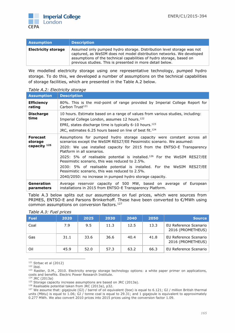
ENER/C1/2015-394

165


Electricity storage Assumed only pumped hydro storage. Distribution level storage was not captured, as WeSIM does not model distribution networks. We developed assumptions of the technical capabilities of hydro storage, based on previous studies. This is presented in more detail below.

We modelled electricity storage using one representative technology, pumped hydro

storage. To do this, we developed a number of assumptions on the technical capabilities

of storage facilities, which are presented in the Table A.2 below.

Table A.2: Electricity storage


Efficiency rating

80%. This is the mid-point of range provided by Imperial College Report for Carbon Trust121

Discharge time

10 hours. Estimate based on a range of values from various studies, including:

Imperial College London, assumes 12 hours.122

EPRI, states discharge time is typically 6-10 hours.123

JRC, estimates 6.25 hours based on line of best fit.124

Forecast storage capacity 125

Assumptions for pumped hydro storage capacity were constant across all scenarios except the WeSIM RES27/EE Pessimistic scenario. We assumed:

2020: We use installed capacity for 2015 from the ENTSO-E Transparency Platform in all scenarios.

2025: 5% of realisable potential is installed.126 For the WeSIM RES27/EE Pessimistic scenario, this was reduced to 2.5%.

2030: 5% of realisable potential is installed. For the WeSIM RES27/EE Pessimistic scenario, this was reduced to 2.5%.

2040/2050: no increase in pumped hydro storage capacity.

Generation parameters

Average reservoir capacity of 500 MW, based on average of European installations in 2015 from ENTSO-E Transparency Platform.

Table A.3 below splits out our assumptions on fuel prices, which were sources from

PRIMES, ENTSO-E and Parsons Brinkerhoff. These have been converted to €/MWh using

common assumptions on conversion factors.127

Table A.3: Fuel prices

Fuel 2020 2025 2030 2040 2050 Source

Coal 7.9 9.5 11.3 12.5 13.3 EU Reference Scenario

2016 (PROMETHEUS)

Gas 31.1 33.6 36.6 40.4 41.8 EU Reference Scenario

2016 (PROMETHEUS)

Oil 45.9 52.0 57.3 63.2 66.3 EU Reference Scenario

121 Strbac et al (2012) 122 Ibid. 123 Rastler, D.M., 2010. Electricity energy storage technology options: a white paper primer on applications, costs and benefits. Electric Power Research Institute. 124 JRC (2013a) 125 Storage capacity increase assumptions are based on JRC (2013a). 126 Realisable potential taken from JRC (2013a), p32. 127 We assume that: gigajoule (GJ) / barrel of oil equivalent (boe) is equal to 6.121; GJ / million British thermal

units (Mbtu) is equal to 1.06; GJ / tonne coal is equal to 29.31; and 1 gigajoule is equivalent to approximately 0.277 MWh. We also convert 2010 prices into 2015 prices using the conversion factor 1.09.

ENER/C1/2015-394

166

Fuel 2020 2025 2030 2040 2050 Source

2016 (PROMETHEUS)

Nuclear 1.7 1.7 1.7 1.7 1.7 ENTSO-E

Biomass 30.5 31.7 32.9 34.5 36.4 Parsons Brinkerhoff

Geothermal 0 0 0 0 0 ENTSO-E

Table A.4 below sets out our assumptions on technology costs (O&M and capex) for RES-

e and conventional generators that was assumed in our modelling. The only caveat to

this table is that we ran a sensitivity on offshore wind capex costs in which cost

reductions were projected to be much more rapid than in the baseline scenario.

Table A.4: Technology costs

2020 2025 2030 2040 2050

Variable O&M (2015 €/kWh)

Solar PV 0 0 0 0 0

Onshore wind 0.0005 0.0005 0.0005 0.0005 0.0005

Offshore wind 0.0005 0.0005 0.0005 0.0005 0.0005

Offshore wind sensitivity 0 0 0 0 0

Biomass 0.004 0.004 0.004 0.004 0.004

Hydro ROR 0 0 0 0 0

Hydro reservoir 0.0003 0.0003 0.0003 0.0003 0.0003

Geothermal 0.0003 0.0003 0.0003 0.0003 0.0003

Wave 0.0001 0.0001 0.0001 0.0001 0.0001

Tidal range 0.0001 0.0001 0.0001 0.0001 0.0001

Nuclear 0.006 0.006 0.007 0.008 0.008

CCGT 0.002 0.002 0.002 0.002 0.002

OCGT 0.002 0.002 0.002 0.002 0.002

Fixed O&M (2015 €/kW)

Solar PV 13.6 12.9 11.9 11.5 10.8

Onshore wind 18.1 18.1 18.1 16.7 18.3

Offshore wind 52.4 49.4 46.3 43.3 41.4


Biomass 47.7 44.0 40.3 39.4 38.6

Hydro ROR 8.9 8.6 8.2 8.2 8.1

Hydro reservoir 25.6 25.6 25.6 25.6 25.6

Geothermal 110.6 110.6 110.6 115.5 120.6

Wave 39.8 36.6 33.5 28.1 23.6

Tidal range 39.8 36.6 33.5 28.1 23.6

Nuclear 120.6 118.0 115.5 108.5 105.5

ENER/C1/2015-394

167

2020 2025 2030 2040 2050

CCGT 22.6 22.2 21.9 21.4 19.4

OCGT 0.002 0.002 0.002 0.002 0.002

Capex costs (2015 €/kW)

Solar PV 845.9 783.6 721.3 668.1 616.2

Onshore wind 1406.4 1381.3 1356.2 1306.0 1285.9

Offshore wind 3495.0 3290.1 3085.1 2888.0 2762.5


Biomass 2662.2 2310.6 1959.0 1808.3 1808.3

Hydro ROR 2461.3 2436.2 2411.0 2360.8 2310.6

Hydro reservoir 3013.8 3013.8 3013.8 3013.8 3013.8

Geothermal 5394.7 5143.6 4892.4 4440.3 4028.5

Wave 6128.1 5475.1 4822.1 3214.7 3114.4

Tidal range 6128.1 5475.1 4822.1 3214.7 3114.3

Nuclear 6831.3 6680.6 6529.9 6529.9 6529.9

CCGT 803.7 803.7 803.7 783.6 783.6

OCGT 1004.6 1004.6 1004.6 1004.6 1004.6

Deployment scenarios

We used PRIMES to calibrate the deployment mix for both renewable and conventional

technologies in EU MS. There were five different deployment scenarios that were used

across our scenarios, as summarised in Table A.5 below and presented in subsequent

charts.

Table A.5: Deployment scenarios

Scenario Deployment scenario

1 WeSIM RES27/EE27 Based on PRIMES EUCO27

2 WeSIM RES27/EE30 Based on PRIMES EUCO30

3 WeSIM RES27/EE Pessimistic Based on PRIMES Reference scenario,

adjusted for increased RES-e penetration

4 WeSIM Ref Based on PRIMES Reference Scenario

5 Lower ETS prices Based on PRIMES EUCO27

6 National CRMs Based on PRIMES EUCO27

7 Removal of preferential market rules Based on PRIMES EUCO27

8 WeSIM RES30/EE30 Based on PRIMES RES3030

9 Imperfect foresight of carbon prices Based on PRIMES EUCO27

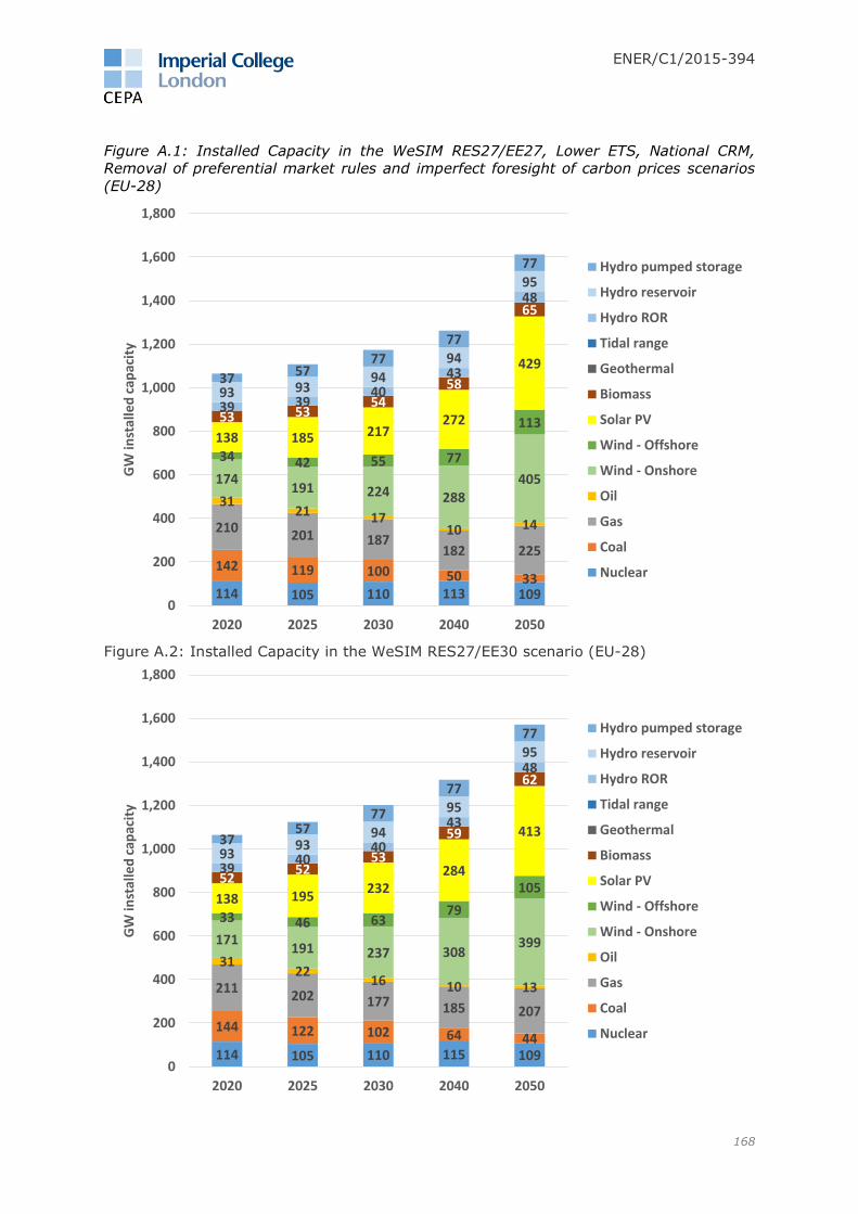
ENER/C1/2015-394

168

Figure A.1: Installed Capacity in the WeSIM RES27/EE27, Lower ETS, National CRM,

Removal of preferential market rules and imperfect foresight of carbon prices scenarios

(EU-28)

Figure A.2: Installed Capacity in the WeSIM RES27/EE30 scenario (EU-28)

114 105 110 113 109

142 119 100 50 33

210201 187

182 225

3121 17

10 14

174191 224 288

405

34 42 55 77

113138 185 217

272

429

53 5354

58

65

39 3940

43

48

93 9394

94

95

37 5777

77

77

0

200

400

600

800

1,000

1,200

1,400

1,600

1,800

2020 2025 2030 2040 2050

GW

inst

alle

d c

apac

ity

Hydro pumped storage

Hydro reservoir

Hydro ROR

Tidal range

Geothermal

Biomass

Solar PV

Wind - Offshore

Wind - Onshore

Oil

Gas

Coal

Nuclear

114 105 110 115 109

144 122 102 64 44

211202 177 185 207

3122

16 10 13

171191 237 308

399

33 46 6379

105138 195

232284

413

5252

53

59

62

3940

40

43

48

9393

94

95

95

3757

77

77

77

0

200

400

600

800

1,000

1,200

1,400

1,600

1,800

2020 2025 2030 2040 2050

GW

inst

alle

d c

apac

ity


Hydro reservoir

Hydro ROR

Tidal range

Geothermal

Biomass

Solar PV

Wind - Offshore

Wind - Onshore

Oil

Gas

Coal

Nuclear

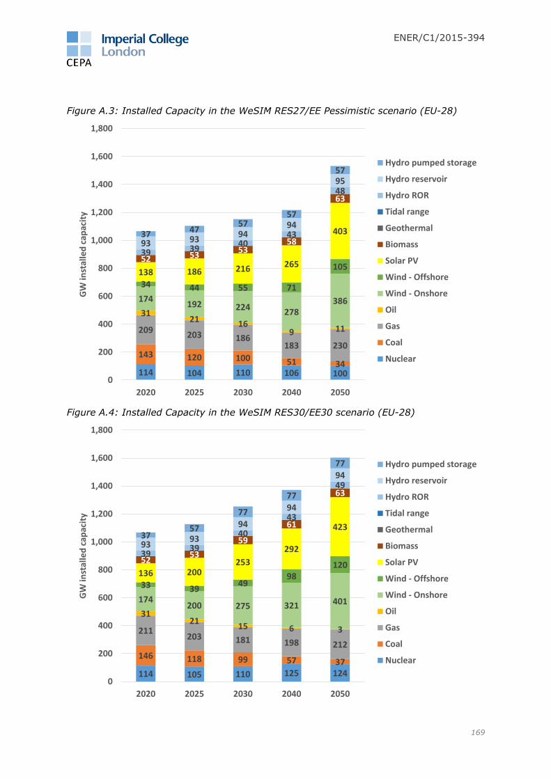
ENER/C1/2015-394

169

Figure A.3: Installed Capacity in the WeSIM RES27/EE Pessimistic scenario (EU-28)

Figure A.4: Installed Capacity in the WeSIM RES30/EE30 scenario (EU-28)

114 104 110 106 100

143 120 100 51 34

209203 186

183 230

3121 16

9 11

174192 224

278386

34 44 55 71

105138 186 216 265

403

52 5353

58

63

39 3940

43

48

93 9394

94

95

37 4757

57

57

0

200

400

600

800

1,000

1,200

1,400

1,600

1,800

2020 2025 2030 2040 2050

GW

inst

alle

d c

apac

ity


Hydro reservoir

Hydro ROR

Tidal range

Geothermal

Biomass

Solar PV

Wind - Offshore

Wind - Onshore

Oil

Gas

Coal

Nuclear

114 105 110 125 124

146 118 99 57 37

211203 181 198 212

3121

15 6 3

174200 275 321 401

33 3949

98120

136 200253

292

423

5253

59

61

63

3939

40

43

49

9393

94

94

94

3757

77

77

77

0

200

400

600

800

1,000

1,200

1,400

1,600

1,800

2020 2025 2030 2040 2050

GW

inst

alle

d c

apac

ity


Hydro reservoir

Hydro ROR

Tidal range

Geothermal

Biomass

Solar PV

Wind - Offshore

Wind - Onshore

Oil

Gas

Coal

Nuclear

ENER/C1/2015-394

170

Figure A.5: Installed Capacity in the WeSIM Ref scenario (EU-28)

For non-EU countries, we developed deployment scenarios based on ENTSO-E TYNDP

2016 forecasts where possible, supplemented by forecasts from National Renewable

Electricity Action Plans (primarily for the Balkan countries). We did not assume any

change in capacity mix after 2030 for these countries. Assumptions on capacity mix for

non-EU countries are set out in the Table A.6 below, and capacity values are shown in

the subsequent chart.

Table A.6: Deployment scenarios

Country Primary data source Additional assumptions

Norway ENTSO-E TYNDP 2016 Assume no offshore wind (based on NREAP).

Switzerland ENTSO-E TYNDP 2016 40% of ‘Other RES’ from ENTSO-E TYNDP2016 is

geothermal (based on current split from Swiss Federal Office of Energy).

60% of ‘Other RES’ from ENTSO-E TYNDP 2016 is biomass (based on current split from Swiss Federal Office of Energy).

All nuclear is decommissioned post-2030 (Swiss policy statement).

Albania ENTSO-E TYNDP 2016 Assume 25% of wind capacity is offshore (based on NREAP).

Bosnia ENTSO-E TYNDP 2016

114 105 110 97 88

144 122 10454 50

210207 192

210 258

3122

179

12

171186

205231

317

3338 38 40

44138 160 179 206

28052 52 53 55

58

39 39 40 42

47

93 93 94 94

94

37 57 77 77

77

0

200

400

600

800

1,000

1,200

1,400

2020 2025 2030 2040 2050

GW

inst

alle

d c

apac

ity


Hydro reservoir

Hydro ROR

Tidal range

Geothermal

Biomass

Solar PV

Wind - Offshore

Wind - Onshore

Oil

Gas

Coal

Nuclear

ENER/C1/2015-394

171

Country Primary data source Additional assumptions

Macedonia ENTSO-E TYNDP 2016 Assume 10 MW of geothermal and 25 MW of biomass in all years (NREAP target).

Montenegro ENTSO-E TYNDP 2016 Assume no offshore wind (based on NREAP).

Serbia ENTSO-E TYNDP 2016

Figure A.6: Installed Capacity for non-EU countries

3 2 1

9 9 9 9 9

1 2 3 3 33 5 6 6 6

2 3 5 5 51 1 1

34

4 4 4

6366

68 68 68

5

5

5 5 5

0

20

40

60

80

100

120

2020 2025 2030 2040 2050

GW

inst

alle

d c

apac

ity


Hydro reservoir

Hydro ROR

Tidal range

Geothermal

Biomass

Solar PV

Wind - Offshore

Wind - Onshore

Oil

Gas

Coal

Nuclear

ENER/C1/2015-394

172

RES-e share of electricity generation in 2030

The PRIMES results used to calibrate our model captured different levels of RES-e and RES-e penetration, as shown in Table A.7 below.

The RES-e penetration was based on estimated generation from PRIMES as a percentage of final energy demand, plus transmission and

distribution losses.

Table A.7: RES target and RES-e penetration across EU28

Scenario 2030 RES target

(% of EU28 primary energy consumption from RES)

Equivalent 2030 RES-e target

(% of EU28 final electricity demand (+ losses) from RES-e)

Source

1 WeSIM RES27/EE27 27% 48%

CEPA – based on PRIMES EUCO27

2 WeSIM RES27/EE30 27% 54%


3 WeSIM RES27/EE Pessimistic 27% 48%

CEPA – based on PRIMES Reference Scenario

4 WeSIM Ref 24% 43%


5 Lower ETS prices 27% 48%


6 National CRMs 27%

48% CEPA – based on PRIMES

EUCO27

7 Removal of preferential market rules 27%

48% CEPA – based on PRIMES EUCO27

8 WeSIM RES30/EE30 30% 57%

CEPA – based on PRIMES RES3030

9 Imperfect foresight of carbon prices 27% 48%


ENER/C1/2015-394

173

Electricity demand

Various PRIMES scenarios were used to calibrate our model for each MS’s annual electricity demand. As an input, WeSIM used data on

final energy demand, plus transmission and distribution losses as a measure for annual electricity demand.

For non-EU states, we used projections from ENTSO-E’s TYNDP 2016, Vision 3. We did not assume any change in annual electricity

demand for non-EU countries after 2030.

Table A.8: Annual electricity demand assumptions

EU 28 Electricity demand (TWh) 2020 2025 2030 2040 2050 Source

1 WeSIM RES27/EE27 3107 3148 3292 3622 3989

CEPA – based on PRIMES

EUCO27

2 WeSIM RES27/EE30 3131 3168 3139 3659 3931 CEPA – based on PRIMES

EUCO30

3 WeSIM RES27/EE Pessimistic 3115 3203 3298 3535 3796

CEPA – based on PRIMES

Reference Scenario

4 WeSIM Ref 3115 3203 3298 3535 3796


5 Lower ETS prices 3107 3148 3292 3622 3989


6 National CRMs 3107 3148 3292 3622 3989


7 Removal of preferential market rules 3107 3148 3292 3622 3989


8 WeSIM RES30/EE30 3138 3212 3143 3714 4022

CEPA – based on PRIMES RES3030

9 Imperfect foresight of carbon prices 3107 3148 3292 3622 3989


Non-EU countries 275 279 282 282 282 ENTSO-E TYNDP 2016

ENER/C1/2015-394

174

Energy Efficiency

Energy efficiency represents changes in total electricity demand versus a pre-defined baseline from 2007 energy consumption statistics.

In WeSIM, difference in energy efficiency flow through to the results by impacting the level of electricity demand. Energy efficiency

assumptions were embedded into the electricity demand values, taken from various PRIMES scenarios (shown in the previous section).

Each PRIMES scenario also captures a variety of other features that influence electricity demand, such as the penetration of electric

vehicles. Therefore, isolating the impact of energy efficiency on electricity demand is difficult. Nonetheless, the levels of energy efficiency

achieved by 2030 in each scenario are as follows:

Table A.9: Energy efficiency by scenario/ sensitivity by 2030

EU 28 Electricity demand (GWh) Energy efficiency achieved by 2030 Source

1 WeSIM RES27/EE27 27% CEPA – based on PRIMES EUCO27

2 WeSIM RES27/EE30 30% CEPA – based on PRIMES EUCO30

3 WeSIM RES27/EE Pessimistic 24% CEPA – based on PRIMES Reference Scenario

4 WeSIM Ref 24%


5 Lower ETS prices 27% CEPA – based on PRIMES EUCO27

6 National CRMs 27% CEPA – based on PRIMES EUCO27

7 Removal of preferential market rules 27% CEPA – based on PRIMES EUCO27

8 WeSIM RES30/EE30 30% CEPA – based on PRIMES RES3030

9 Imperfect foresight of carbon prices 27% CEPA – based on PRIMES EUCO27

Interconnection capacity128

We calibrated interconnection capacity in WeSIM using ENTSO-E’s TYNDP 2016. Assumptions on transmission capacity were equivalent

across scenarios/ sensitivities, apart from the WeSIM RES27/EE Pessimistic scenario in which we assumed no new interconnection in

128 WeSIM endogenously adds additional interconnection capacity, on top of the interconnection capacity assumed by ENTSO-E, for all scenarios and years modelled if it is efficient to do so.

ENER/C1/2015-394

175

2025. As part of WeSIM’s cost minimisation algorithm, WeSIM also endogenously adds additional interconnection capacity if it was

efficient to do so.

We made the following assumptions:

2020: Used ENTSO-E reference interconnection capacities for 2020 as an input into WeSIM.

2025: Transmission capacity of projects of common interest (PCIs) with a commissioning date on or before 2025 were added to

the 2020 capacity values. Capacity and commissioning dates for PCIs were taken from ENTSO-E TYNDP 2016. The WeSIM

RES27/EE Pessimistic scenario assumed no new interconnection.

2030: Used ENTSO-E interconnection capacities for 2030 as an input into WeSIM.

2040/50: Assumed no additional interconnection capacity was assumed to have been installed after 2030. We relied purely on

WeSIM’s optimisation process to forecast additions to interconnection capacity.

The interconnection inputs to WeSIM are presented in Table A.10 below. Another important input into WeSIM is the assumed distances

between nodes (countries) in its network and the cost of new interconnection. Distances were estimated "as the crow flies" between two

locations in each country, typically a middle point within the country). Costs of new interconnection were based on previous Commission

studies and were provided by Imperial College London. We cross-checked these values by comparing them to a selection of projects in

ENTSO-E’s TYNDP2014.

Table A.10: Interconnection capacity assumptions

Total

interconnection

capacity (MW)

2020 2025 2030 2040 2050

Austria 10655 14255 14255 14255 14255

Belgium 8280 8280 8280 8280 8280

Bulgaria 4258 4258 4258 4258 4258

Croatia 5912 5912 6412 6412 6412

Cyprus 2000 2000 2000 2000 2000

Czech Republic 5900 6200 6400 6400 6400

Denmark 10180 10180 10180 10180 10180

Estonia 2616 2616 2616 2616 2616

ENER/C1/2015-394

176

Total

interconnection

capacity (MW)

2020 2025 2030 2040 2050

Finland 3300 3800 3800 3800 3800

France 20730 23730 26230 26230 26230

Germany 28551 32251 34601 34601 34601

Greece 4132 4132 4132 4132 4132

Hungary 8400 8400 8400 8400 8400

Ireland 5980 7100 7100 7100 7100

Italy 9685 10685 10685 10685 10685

Latvia 2800 3400 3400 3400 3400

Lithuania 3200 3800 3800 3800 3800

Luxembourg 3000 3000 3000 3000 3000

Malta 200 200 200 200 200

Netherlands 9250 9250 9800 9800 9800

Poland 6190 6190 6190 6190 6190

Portugal 3500 3500 3500 3500 3500

Romania 4350 4350 4350 4350 4350

Slovakia 4090 4090 4090 4090 4090

Slovenia 6730 6730 6730 6730 6730

Spain 9200 11200 12200 12200 12200

Sweden 10290 11790 11790 11790 11790

UK 11200 11200 11200 11200 11200

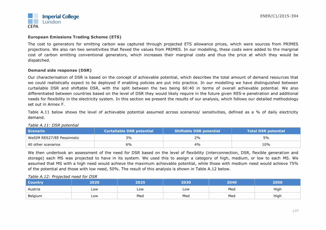
ENER/C1/2015-394

177

European Emissions Trading Scheme (ETS)

The cost to generators for emitting carbon was captured through projected ETS allowance prices, which were sources from PRIMES

projections. We also ran two sensitivities that flexed the values from PRIMES. In our modelling, these costs were added to the marginal

cost of carbon emitting conventional generators, which increases their marginal costs and thus the price at which they would be

dispatched.

Demand side response (DSR)

Our characterisation of DSR is based on the concept of achievable potential, which describes the total amount of demand resources that

we could realistically expect to be deployed if enabling policies are put into practice. In our modelling we have distinguished between

curtailable DSR and shiftable DSR, with the split between the two being 60:40 in terms of overall achievable potential. We also

differentiated between countries based on the level of DSR they would likely require in the future given RES-e penetration and additional

needs for flexibility in the electricity system. In this section we present the results of our analysis, which follows our detailed methodology

set out in Annex F.

Table A.11 below shows the level of achievable potential assumed across scenarios/ sensitivities, defined as a % of daily electricity

demand.

Table A.11: DSR potential

Scenario Curtailable DSR potential Shiftable DSR potential Total DSR potential

WeSIM RES27/EE Pessimistic 3% 2% 5%

All other scenarios 6% 4% 10%

We then undertook an assessment of the need for DSR based on the level of flexibility (interconnection, DSR, flexible generation and

storage) each MS was projected to have in its system. We used this to assign a category of high, medium, or low to each MS. We

assumed that MS with a high need would achieve the maximum achievable potential, while those with medium need would achieve 75%

of the potential and those with low need, 50%. The result of this analysis is shown in Table A.12 below.

Table A.12: Projected need for DSR

Country 2020 2025 2030 2040 2050

Austria Low Low Low Med High

Belgium Low Med Med Med High

ENER/C1/2015-394

178

Country 2020 2025 2030 2040 2050

Bulgaria Low Med Med High High

Cyprus Low Low Low Low High

Czech Republic Low Low Low Low Med

Denmark Low Med Med Med High

Estonia Low Low Low Med High

Finland Low Low Low Low Med

France Med Med Med High High

Germany High High High High High

Greece Low Med High High High

Croatia Low Low Low Low Med

Hungary Low Low Low Low Low

Ireland High High High High High

Italy Low Med Med High High

Latvia Low Low Low Low Med

Luxembourg Low Low Low Low Low

Malta Low Low Low Med High

Lithuania Low Low Low Low High

Netherlands High High High High High

Poland Med Med Med High High

Portugal Low Med Med High High

Romania Low Low Med High High

Slovakia Low Low Low Low Low

Slovenia Low Low Low Low Low

ENER/C1/2015-394

179

Country 2020 2025 2030 2040 2050

Spain Med High High High High

Sweden Low Low Low Low Med

UK High High High High High

We then took into account the speed at which countries would be able to implement policies that promote DSR as well as whether each

country’s industrial sector (a large contributor to DSR) was large enough to support material volumes of DSR. The results of our analysis

are a set of percentages (of daily demand) representing an estimate of the DSR potential achieved by each country. The results for the

WeSIM RES27/EE27 scenario are shown in Table A.13 below (WeSIM RES27/EE Pessimistic scenario values are half of those presented

below).

Table A.13: DSR resources deployed (% of daily load) by MS

Country 2020 2025 2030 2040 2050

Austria 5% 5% 5% 8% 10%

Belgium 5% 8% 8% 8% 10%

Bulgaria 3% 8% 8% 10% 10%

Cyprus 1% 5% 5% 5% 5%

Czech Republic 5% 5% 5% 5% 8%

Denmark 3% 8% 8% 8% 10%

Estonia 5% 5% 5% 8% 10%

Finland 5% 5% 5% 5% 8%

France 5% 8% 8% 10% 10%

Germany 3% 10% 10% 10% 10%

Greece 3% 8% 10% 10% 10%

Croatia 3% 5% 5% 5% 5%

Hungary 5% 5% 5% 5% 5%

ENER/C1/2015-394

180

Country 2020 2025 2030 2040 2050

Ireland 5% 10% 10% 10% 10%

Italy 3% 8% 8% 10% 10%

Latvia 5% 5% 5% 5% 8%

Luxembourg 5% 5% 5% 5% 5%

Malta 3% 5% 5% 5% 5%

Lithuania 5% 5% 5% 5% 10%

Netherlands 5% 10% 10% 10% 10%

Poland 3% 8% 8% 10% 10%

Portugal 5% 8% 8% 10% 10%

Romania 5% 5% 8% 10% 10%

Slovakia 3% 5% 5% 5% 5%

Slovenia 3% 5% 5% 5% 5%

Spain 3% 10% 10% 10% 10%

Sweden 5% 5% 5% 5% 8%

UK 5% 10% 10% 10% 10%

Capacity remuneration markets (CRM)

Capacity remuneration mechanisms are mechanisms that allow generators to make revenues for being available to generate. They are

used as a way to procure capacity and allow generators to recover fixed costs through a more reliable stream of payments than would be

the case with energy only markets. This helps to avoid times of tightness in the electricity system, which would otherwise produce

scarcity prices (i.e., prices that exceed the marginal cost of the most expensive generator).

We modelled CRMs as a sensitivity to the WeSIM RES27/EE27 scenario. From this scenario we repackage revenues from times of scarcity

and redistribute them based on generators’ contribution to capacity during those times. We therefore only model national CRMs in

countries, which exhibit periods of scarcity throughout the year (in the WeSIM RES27/EE27 scenario). Table A.14 below provides a list of

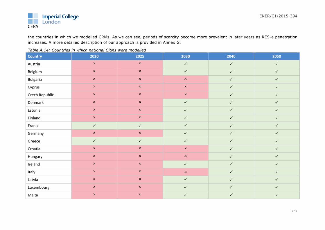
ENER/C1/2015-394

181

the countries in which we modelled CRMs. As we can see, periods of scarcity become more prevalent in later years as RES-e penetration

increases. A more detailed description of our approach is provided in Annex G.

Table A.14: Countries in which national CRMs were modelled

Country 2020 2025 2030 2040 2050

Austria

Belgium

Bulgaria

Cyprus

Czech Republic

Denmark

Estonia

Finland

France

Germany

Greece

Croatia

Hungary

Ireland

Italy

Latvia

Luxembourg

Malta

ENER/C1/2015-394

182

Country 2020 2025 2030 2040 2050

Lithuania

Netherlands

Poland

Portugal

Romania

Slovakia

Slovenia

Spain

Sweden

UK

ENER/C1/2015-394

183


Priority dispatch is a market access rule, which places an obligation on TSOs to schedule

and dispatch RES-e generators ahead of all other types of generation. The purpose of

priority dispatch is to provide certainty to renewable generators that they will be able to

sell electricity into the grid at all times (reducing volume risk) and to enable a more

rapid integration of RES-e generators into the power system.

Currently, priority dispatch is being combined with other forms of support (e.g., FITs &

CfDs in UK) that make it profitable to sell electricity on the wholesale market at any price

(even below marginal cost). It is implemented for renewable electricity generators, but is

relevant only for those with non-zero marginal costs, namely biomass.

As a baseline assumption we assumed that renewable would continue to receive priority

dispatch indefinitely. Using the WeSIM RES27/EE27 scenario as a baseline, we then

conducted a sensitivity in which we removed priority dispatch for all renewables from

2020 onwards. This was done only for one sensitivity, all other scenarios/sensitivities

assumed priority dispatch continued.

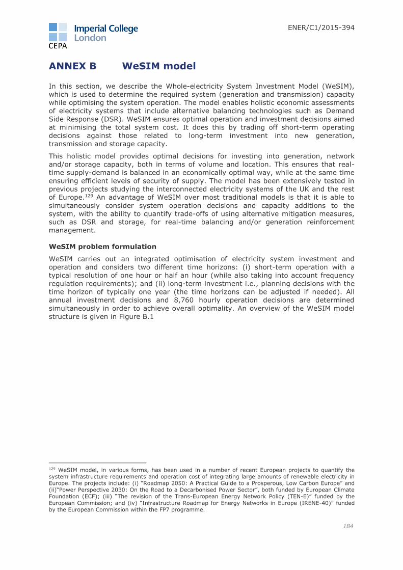
ENER/C1/2015-394

184

ANNEX B WeSIM model

In this section, we describe the Whole-electricity System Investment Model (WeSIM),

which is used to determine the required system (generation and transmission) capacity

while optimising the system operation. The model enables holistic economic assessments

of electricity systems that include alternative balancing technologies such as Demand

Side Response (DSR). WeSIM ensures optimal operation and investment decisions aimed

at minimising the total system cost. It does this by trading off short-term operating

decisions against those related to long-term investment into new generation,

transmission and storage capacity.

This holistic model provides optimal decisions for investing into generation, network

and/or storage capacity, both in terms of volume and location. This ensures that real-

time supply-demand is balanced in an economically optimal way, while at the same time

ensuring efficient levels of security of supply. The model has been extensively tested in

previous projects studying the interconnected electricity systems of the UK and the rest

of Europe.129 An advantage of WeSIM over most traditional models is that it is able to

simultaneously consider system operation decisions and capacity additions to the

system, with the ability to quantify trade-offs of using alternative mitigation measures,

such as DSR and storage, for real-time balancing and/or generation reinforcement

management.

WeSIM problem formulation

WeSIM carries out an integrated optimisation of electricity system investment and

operation and considers two different time horizons: (i) short-term operation with a

typical resolution of one hour or half an hour (while also taking into account frequency

regulation requirements); and (ii) long-term investment i.e., planning decisions with the

time horizon of typically one year (the time horizons can be adjusted if needed). All

annual investment decisions and 8,760 hourly operation decisions are determined

simultaneously in order to achieve overall optimality. An overview of the WeSIM model

structure is given in Figure B.1

129 WeSIM model, in various forms, has been used in a number of recent European projects to quantify the system infrastructure requirements and operation cost of integrating large amounts of renewable electricity in Europe. The projects include: (i) “Roadmap 2050: A Practical Guide to a Prosperous, Low Carbon Europe” and (ii)“Power Perspective 2030: On the Road to a Decarbonised Power Sector”, both funded by European Climate Foundation (ECF); (iii) “The revision of the Trans-European Energy Network Policy (TEN-E)” funded by the

European Commission; and (iv) “Infrastructure Roadmap for Energy Networks in Europe (IRENE-40)” funded by the European Commission within the FP7 programme.

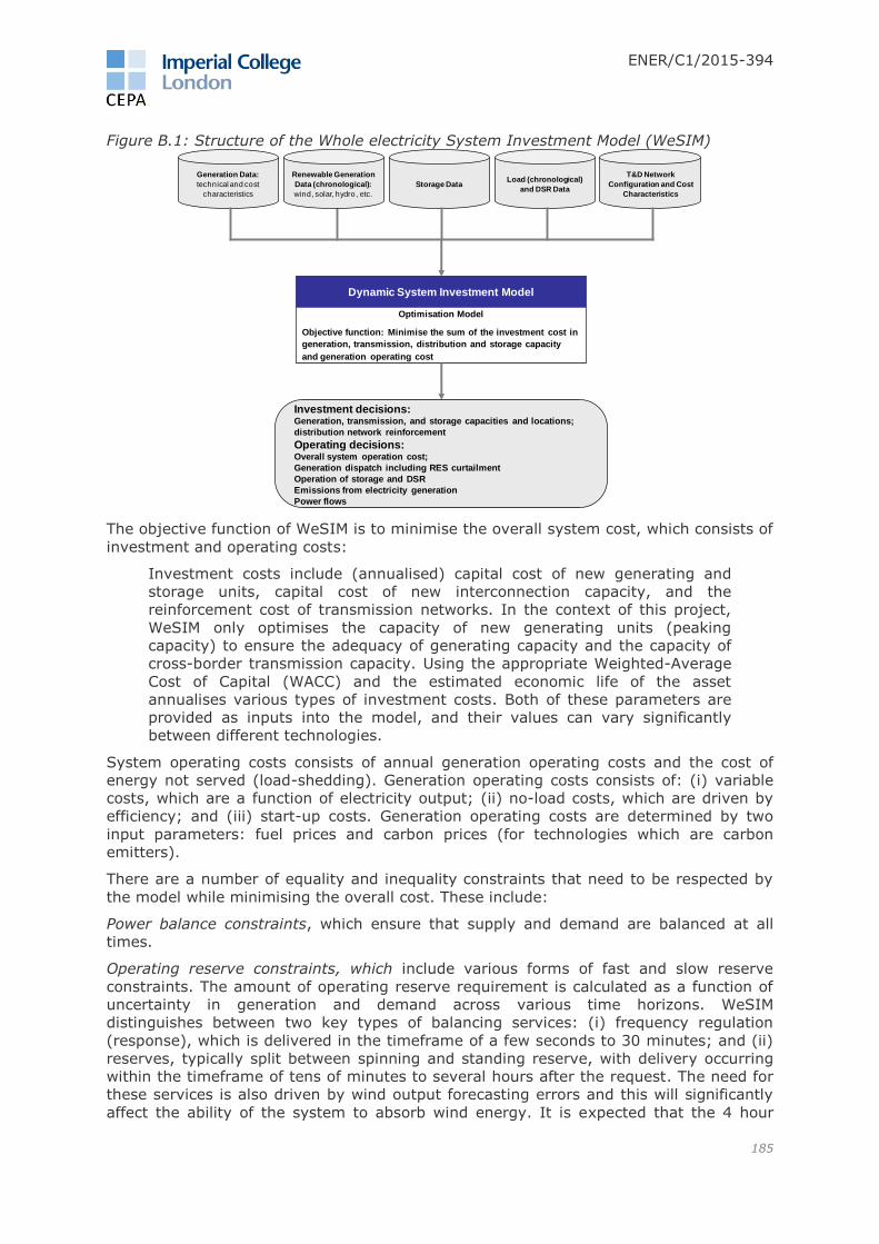
ENER/C1/2015-394

185

Figure B.1: Structure of the Whole electricity System Investment Model (WeSIM)

The objective function of WeSIM is to minimise the overall system cost, which consists of

investment and operating costs:

Investment costs include (annualised) capital cost of new generating and

storage units, capital cost of new interconnection capacity, and the

reinforcement cost of transmission networks. In the context of this project,

WeSIM only optimises the capacity of new generating units (peaking

capacity) to ensure the adequacy of generating capacity and the capacity of

cross-border transmission capacity. Using the appropriate Weighted-Average

Cost of Capital (WACC) and the estimated economic life of the asset

annualises various types of investment costs. Both of these parameters are

provided as inputs into the model, and their values can vary significantly

between different technologies.

System operating costs consists of annual generation operating costs and the cost of

energy not served (load-shedding). Generation operating costs consists of: (i) variable

costs, which are a function of electricity output; (ii) no-load costs, which are driven by

efficiency; and (iii) start-up costs. Generation operating costs are determined by two

input parameters: fuel prices and carbon prices (for technologies which are carbon

emitters).

There are a number of equality and inequality constraints that need to be respected by

the model while minimising the overall cost. These include:

Power balance constraints, which ensure that supply and demand are balanced at all

times.

Operating reserve constraints, which include various forms of fast and slow reserve

constraints. The amount of operating reserve requirement is calculated as a function of

uncertainty in generation and demand across various time horizons. WeSIM

distinguishes between two key types of balancing services: (i) frequency regulation

(response), which is delivered in the timeframe of a few seconds to 30 minutes; and (ii)

reserves, typically split between spinning and standing reserve, with delivery occurring

within the timeframe of tens of minutes to several hours after the request. The need for

these services is also driven by wind output forecasting errors and this will significantly

affect the ability of the system to absorb wind energy. It is expected that the 4 hour

Generation Data:

technical and cost

characteristics

Renewable Generation

Data (chronological):

wind, solar, hydro , etc.

Storage DataLoad (chronological)

and DSR Data

T&D Network

Configuration and Cost

Characteristics

Dynamic System Investment Model

Optimisation Model

Objective function: Minimise the sum of the investment cost in

generation, transmission, distribution and storage capacity

and generation operating cost

Investment decisions: Generation, transmission, and storage capacities and locations;

distribution network reinforcement

Operating decisions:Overall system operation cost;

Generation dispatch including RES curtailment

Operation of storage and DSR

Emissions from electricity generation

Power flows

ENER/C1/2015-394

186

ahead130 forecasting error of wind, being at present at about 15% of installed wind

capacity, may reduce to 10% post-2020 and then further to less than 6%. This may

have a material impact on the value of flexibility options. Calculation of reserve and

response requirements for a given level of intermittent renewable generation is carried

out exogenously and provided as an input into the model. WeSIM then schedules the

optimal provision of reserve and response services, taking into account the capabilities

and costs of potential providers of these services (response slopes, efficiency losses of

part loaded plant etc.). Following on, WeSIM finds the optimal trade-off between the cost

of generating electricity to supply a given demand profile, and the cost of procuring

sufficient levels of reserve and response (this also includes alternative balancing

technologies such as storage and DSR as appropriate).

In WeSIM, frequency response can be provided by:

Synchronised part-loaded generating units;

Interruptible charging of electric vehicles;

A proportion of wind power being curtailed;

Electricity storage; and

Flexible and controllable demand such as Electric Vehicles and smart appliances.

While reserve services can be provided by:

Synchronised generators;

Wind power or solar power being curtailed;

Stand-by fast generating units (OCGT);

Electricity storage; and

Flexible demand.

The amount of spinning and standing reserve and response is optimised ex-ante to

minimise the expected cost of providing these services, and we use our advanced

stochastic generation scheduling models to calibrate the amount of reserve and response

scheduled in WeSIM.131,132 These models find the cost-optimal levels of reserve and

response by performing a probabilistic simulation of the actual utilisation of these

services. Stochastic scheduling is particularly important when allocating storage

resources between energy arbitrage and reserve as this may vary dynamically depending

on the system conditions.

Generator operating constraints include:

(i) Minimum Stable Generation (MSG) and maximum output constraints;

(ii) ramp-up and ramp-down constraints;

(iii) minimum up and down time constraints; and

(iv) available frequency response and reserve constraints.

In order to keep the size of the problem manageable, we group generators according to

technologies, and assume a generic size of a thermal unit of 500 MW (the model can

however commit response services to deal with larger losses, e.g., 1,800 MW as used in

the model). The model captures the fact that the provision of frequency response is

more demanding than providing operating reserve. Only a proportion of the headroom

created by part-loaded operation, as indicated in Figure B.2.

Given that the functional relationship between the available response and the reduced

generation output has a slope with an absolute value considerably lower than 1, the

130 4 hours is generally the maximum time needed to synchronize a large CCGT plant. 131 Sturt and Strbac (2012a) 132 Sturt and Strbac (2012b)

ENER/C1/2015-394

187

maximum amount of frequency regulation that a generator can provide (Rmax) is

generally lower than the headroom created from part-loaded operation (Pmax – MSG).

Figure B.2: Provision of frequency regulation from conventional generation

Generation: WeSIM optimises the investment in new generation capacity while

considering the generators’ operation costs and CO2 emission constraints, and

maintaining the required levels of security of supply. WeSIM optimises both the quantity

and the location of new generation capacity as part of the overall cost minimisation. If

required, the model can limit the investment in particular generation technologies at

given locations.

Annual load factor constraints can be used to limit the utilisation level of thermal

generating units, e.g., to account for the effect of planned annual maintenance on plant

utilisation.

For wind, solar, marine, and hydro ROR generators, the maximum electricity production

is limited by the available energy profile, which is specified as part of the input data. The

model will maximise the utilisation of these units (given zero or low marginal cost). In

certain conditions when there is oversupply of electricity in the system or

reserve/response requirements limit the amount of renewable generation that can be

accommodated, it might become necessary to curtail their electricity output in order to

balance the system.

For hydro generators with reservoirs and pumped-storage units, the electricity

production is limited not only by their maximum power output, but also by the energy

available in the reservoir at a particular time (while optimising the operation of storage).

The amount of energy in the reservoir at any given time is limited by the size of the

reservoir. It is also possible to apply minimum energy constraints in WeSIM to ensure

that a minimum amount of energy is maintained in the reservoir, for example to ensure

the stability of the plant. For storage technologies, WeSIM takes into account efficiency

losses.

Demand side response constraints include constraints for various specific types of loads.

Different demand categories can be modelled with different levels of flexibility, which can

be regional/country and technology specific. Flexibility parameters associated with

various forms of DSR are obtained using detailed bottom-up modelling of different types

of flexible demand. The flexibility of demand is presented in two ways: (i) load-shifting

capability where part of the load during peak hours can be shifted to off-peak hours.

Losses due to temporal shifting of demand are modelled as appropriate, (ii) load

curtailment where some load can be curtailed if it is economic to do so. The cost of load

curtailment becomes part of the system operation cost which is minimised by the model.

Power flow constraints limit the energy flowing through the lines between the areas in

the system, respecting the installed capacity of network as the upper bound. The model

can also invest in enhancing network capacity if this is cost efficient. Expanding

transmission and interconnection capacity is generally found to be vital for facilitating

efficient integration of large intermittent renewable resources, given their location.

ENER/C1/2015-394

188

Interconnectors provide access to renewable energy and improve the diversity of

demand and renewable output on both sides of the interconnector, thus reducing the

short-term reserve requirement. Interconnection also allows for sharing of reserves,

which reduces the long-term capacity requirements.

Security constraints ensure that there is sufficient generating capacity in the system to

supply the demand with a given level of security.133 If there is storage in the system,

WeSIM may use its capacity for security purposes if it can contribute to reducing peak

demand.

WeSIM allows for the security-related benefits of interconnection to be adequately

quantified.134 Conversely, it is possible to specify in WeSIM that no contribution to

security is allowed from other regions. This will clearly increase the system cost but will

also provide an estimate of the value of allowing the interconnection to be used for

sharing security between regions.

133 Historical level of security supply are achieved by setting VOLL at around 10,000£/MWh. 134 Castro et al (2011)

ENER/C1/2015-394

189

ANNEX C Discount rates To conduct the viability analysis used in this study we generated discount rate estimates

for each combination of support option, technology, country and year included in our

analysis.

We anchored our discount rate estimates on the core case of a generic conventional

generator in a AAA-rated country without financial support. We used a pre-tax real

weighted average cost of capital (WACC) framework to structure these estimates and the

capital asset pricing model (CAPM) to estimate the cost of equity portion of it. This

approach provided a clear basis to make adjustments to capture:

the dimension of time; and

differences between countries.

We made further discretionary adjustments to the core estimates to capture the relative

risk of RES-e technologies and support options.

Cost of debt

Contemporary estimates of the cost of debt were generated using the average nominal

yield on iBoxx benchmark euro-denominated BBB 10yr+ non-financial corporate yields

for December 2015 (3.20%),135 supplemented by a 125 basis point spread to produce

estimates approximately in line with a BB rating.

To generate estimates of the cost of debt for the future dates considered in this study, a

further adjustment was made using forward rates calculated from the EC AAA-rated Euro area yield curve (e.g., 3.20% + 1.45% = 4.65% for 2030).136 Figure C.1 below illustrates

how nominal and real forward rates were constructed for this purpose.

Figure C.1: Eurozone AAA sovereign yield curve analysis

Source: CEPA analysis of iBoxx and ECB data

To make country-specific adjustments, a simple country risk premium was added to the

cost of debt using Damadoran 2016 estimates based on local sovereign credit ratings

135 iBoxx benchmark indices were accessed through Markit at https://www.markit.com/Product/IBoxx. 136 Euro area yield curves were accessed from the ECB at https://www.ecb.europa.eu/stats/money/yc/html/index.en.html.

-2.5%

-2.0%

-1.5%

-1.0%

-0.5%

0.0%

0.5%

1.0%

1.5%

2.0%

2.5%

Nominal forward Nominal 1yr Nominal 10yr

Real forward Real 1yr% Real 10yr

Infl. Exp 1yr Infl. Exp 10yr

https://www.markit.com/Product/IBoxx

https://www.markit.com/Product/IBoxx

https://www.ecb.europa.eu/stats/money/yc/html/index.en.html

ENER/C1/2015-394

190

(e.g., 3.20% + 1.45% + 0.55% = 5.12% for France in 2030).137 Given the long time

horizon considered, we made adjustments to taper out the effect of any ongoing or

recent crises. To do so, we made the assumption that by 2025 countries’ credit ratings

would have gradually converged to their median level observed since 2000. A further 20

basis point adjustment was added to capture cost of raising debt finance.

To generate an estimate in real terms, all nominal values were deflated using 10-year

forward inflation expectations constructed from ECB 2016 Q1 consensus inflation forecasts (e.g., 1.80% inflation expectations in 2030, resulting in a 3.26% real cost of debt for

France in 2030).138

Adjustments for technology and support schemes were made through the gearing

assumption set at the maximum level consistent with the assumed credit rating. Where

development finance was modelled, we fixed the equity beta used in the CAPM cost of

equity estimate and considered the impact of a five percentage point increase in gearing

as a lower scenario and a ten percentage point increase as a higher scenario.

Cost of equity

A long-term CAPM-based estimate formed the core cost of equity for our analysis using

a:

long-term real risk-free rate (1.36%) set using ten-year average of 20-year AAA-

rated EU sovereign debt (3.39%) deflated using the ECB inflation target (2.00%);

market risk premium (4.5%) set consistent with the 2015 Dimson Marsh and

Staunton estimate of the long-term arithmetic mean of world real equity premia

over bonds;

midpoint CEPA estimate of conventional generator asset beta (0.55) used as a

reference; and

country risk premium as per the cost of debt.

A post-tax unlevered specific risk adjustment determined as part of a separate

calibration process was added to the CAPM-based estimate. The combined real post-tax

cost of equity was converted to nominal terms before grossing-up for country-specific

tax rates (EC 2014 effective tax rates values). Adjustments for technology and support

were made through the beta (for non-diversifiable risks) and the specific risk adjustment

(for diversifiable investor-specific risks).

When carbon contracting was modelled, we made a reduction to the asset beta based on

20 percent of the difference between the value for Fixed FIP and FIT, where 20 percent

is an approximation of the share of revenue related to the carbon price.

Relative risk analysis

To inform our estimates for different combinations of technologies and support options

we conducted qualitative relative risk analysis for each technology (cf. the core

conventional generator assumed) and support option (cf. FIT). As shown in Figure C.2

below, we performed relative risk analysis along three dimensions that would fed

through to specific cost of capital parameters and constraining where adjustments could

be made. This analysis included consideration of how factors such as investor

perceptions of technology maturity might change over time.

137 Damodaran estimates are accessed through Damodaran Online at http://pages.stern.nyu.edu/~adamodar/. 138 ECB consensus forecasts were accessed from the ECB at http://www.ecb.europa.eu/stats/prices/indic/forecast/html/table_3_2016q1.en.html

http://pages.stern.nyu.edu/~adamodar/

http://www.ecb.europa.eu/stats/prices/indic/forecast/html/table_3_2016q1.en.html

ENER/C1/2015-394

191

Figure C.2: Relative risk analysis approach

Further detail on our relative risk analysis is provided in Annex E.

Calibration of quantitative estimates

Qualitative relative risk analysis provided a framework within which it was possible to

estimate quantitative differences in discount rates between different technologies and

support options. Use of external top-down estimates of discount rates provided

important reference points to attribute quantitative estimates in this exercise.

As shown in Figure C.3 below, as part of this process separate risk scores and

coefficients were calculated for the dimensions of technology and support option.

Together, these produced a structured set of estimates that could be calibrated against

other sources while allowing some explanatory power for cases where comparators were

not available.

Figure C.3: Discount rate calibration

A set of discount rate outputs generated using this approach were presented at the

finance workshop held as part of this study, leading to a small number of adjustments as

described in Section 4.2.1. Also, as described in Section 3.2.8, we developed two

1. Cost of debt• Assessment based on Moody’s

power generation rating methodology capturing:• Predictability of cashflows• Regulatory support• Technology and operating

risks

2. Non-diversifiable risk• Focus on risks captured in the

CAPM framework and the degree to which expected to be correlated with overall market.

• Assume differences are permanent.

3. Diversifiable risk• Capture risks that do not fit into

CAPM but literature suggests feature in hurdle rates in practice.

• Key element is technology maturity.

• A more complex approach might reflect these in cashflow scenarios.

Gearing Asset beta Investor premium

Qualitative overall scoring converted to scorese.g. = -1, = +2.5

Relative coefficient e.g. 5% gearing or 0.1 on asset

beta

Estimated component value

NERA (2013) IJGlobal database

Our relative risk analysis was directionalwith limited ability to assess magnitudes

Diacore (2016)

Oxera (2011)

x =

CEPA (2011)

Updated discount rateCalibration gives

the relative analysis quantitative impact

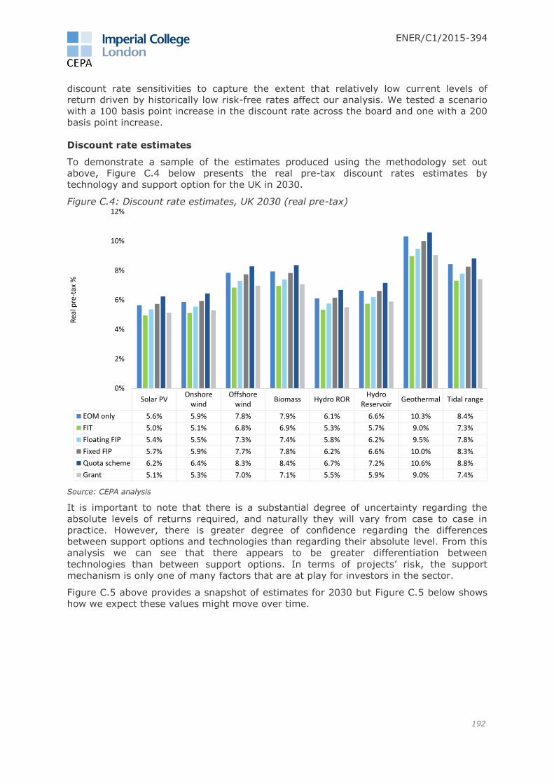
ENER/C1/2015-394

192

discount rate sensitivities to capture the extent that relatively low current levels of

return driven by historically low risk-free rates affect our analysis. We tested a scenario

with a 100 basis point increase in the discount rate across the board and one with a 200

basis point increase.

Discount rate estimates

To demonstrate a sample of the estimates produced using the methodology set out

above, Figure C.4 below presents the real pre-tax discount rates estimates by

technology and support option for the UK in 2030.

Figure C.4: Discount rate estimates, UK 2030 (real pre-tax)


It is important to note that there is a substantial degree of uncertainty regarding the

absolute levels of returns required, and naturally they will vary from case to case in

practice. However, there is greater degree of confidence regarding the differences

between support options and technologies than regarding their absolute level. From this

analysis we can see that there appears to be greater differentiation between

technologies than between support options. In terms of projects’ risk, the support

mechanism is only one of many factors that are at play for investors in the sector.

Figure C.5 above provides a snapshot of estimates for 2030 but Figure C.5 below shows

how we expect these values might move over time.

Solar PVOnshore

windOffshore

windBiomass Hydro ROR

HydroReservoir

Geothermal Tidal range

EOM only 5.6% 5.9% 7.8% 7.9% 6.1% 6.6% 10.3% 8.4%

FIT 5.0% 5.1% 6.8% 6.9% 5.3% 5.7% 9.0% 7.3%

Floating FIP 5.4% 5.5% 7.3% 7.4% 5.8% 6.2% 9.5% 7.8%

Fixed FIP 5.7% 5.9% 7.7% 7.8% 6.2% 6.6% 10.0% 8.3%

Quota scheme 6.2% 6.4% 8.3% 8.4% 6.7% 7.2% 10.6% 8.8%

Grant 5.1% 5.3% 7.0% 7.1% 5.5% 5.9% 9.0% 7.4%

0%

2%

4%

6%

8%

10%

12%

Rea

l pre

-tax

%

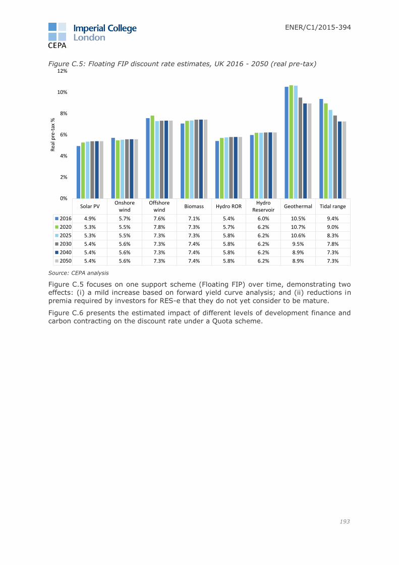
ENER/C1/2015-394

193

Figure C.5: Floating FIP discount rate estimates, UK 2016 - 2050 (real pre-tax)


Figure C.5 focuses on one support scheme (Floating FIP) over time, demonstrating two

effects: (i) a mild increase based on forward yield curve analysis; and (ii) reductions in

premia required by investors for RES-e that they do not yet consider to be mature.

Figure C.6 presents the estimated impact of different levels of development finance and

carbon contracting on the discount rate under a Quota scheme.

Solar PVOnshore

windOffshore


HydroReservoir


2016 4.9% 5.7% 7.6% 7.1% 5.4% 6.0% 10.5% 9.4%

2020 5.3% 5.5% 7.8% 7.3% 5.7% 6.2% 10.7% 9.0%

2025 5.3% 5.5% 7.3% 7.3% 5.8% 6.2% 10.6% 8.3%

2030 5.4% 5.6% 7.3% 7.4% 5.8% 6.2% 9.5% 7.8%

2040 5.4% 5.6% 7.3% 7.4% 5.8% 6.2% 8.9% 7.3%

2050 5.4% 5.6% 7.3% 7.4% 5.8% 6.2% 8.9% 7.3%

0%

2%

4%

6%

8%

10%

12%

Rea

l pre

-tax

%

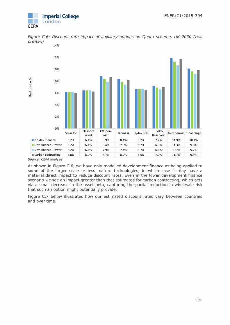
ENER/C1/2015-394

194

Figure C.6: Discount rate impact of auxiliary options on Quota scheme, UK 2030 (real

pre-tax)


As shown in Figure C.6, we have only modelled development finance as being applied to

some of the larger scale or less mature technologies, in which case it may have a

material direct impact to reduce discount rates. Even in the lower development finance

scenario we see an impact greater than that estimated for carbon contracting, which acts

via a small decrease in the asset beta, capturing the partial reduction in wholesale risk

that such an option might potentially provide.

Figure C.7 below illustrates how our estimated discount rates vary between countries

and over time.

Solar PVOnshore

windOffshore


HydroReservoir


No dev. finance 6.2% 6.4% 8.9% 8.4% 6.7% 7.2% 11.9% 10.1%

Dev. finance - lower 6.2% 6.4% 8.4% 7.9% 6.7% 6.9% 11.3% 9.6%

Dev. finance - lower 6.2% 6.4% 7.9% 7.4% 6.7% 6.6% 10.7% 9.2%

Carbon contracting 6.0% 6.2% 8.7% 8.2% 6.5% 7.0% 11.7% 9.9%

0%

2%

4%

6%

8%

10%

12%

14%

Rea

l pre

-tax

%

ENER/C1/2015-394

195

Figure C.7: Onshore wind Floating FIP discount 2016 - 2050, selected countries (real

pre-tax)


In our estimates, differences between countries were driven by corporate tax levels and

country risk premia based on sovereign default risk. Some countries currently have

relatively high sovereign risk captured in their discount rates. However, analysis of

sovereign ratings over time and the long time horizon of this study suggested that it

may not be reasonable to assume that current issues will persist until 2050. As such, we

have modelled current premia to converge to longer-term levels within the next ten

years.

Figure C.8 presents a comparison of discount rates between a national (MS) and EU-wide

(EU) version of three support options in Cyprus in 2020.

Germany Ireland Greece Portugal Spain

2016 5.4% 6.9% 17.3% 8.4% 8.0%

2020 5.3% 6.3% 12.3% 7.4% 7.0%

2025 5.6% 5.9% 6.5% 6.5% 6.4%

2030 5.7% 6.0% 6.6% 6.5% 6.4%

2040 5.7% 6.0% 6.6% 6.5% 6.4%

2050 5.7% 6.0% 6.6% 6.5% 6.4%

0%

2%

4%

6%

8%

10%

12%

14%

16%

18%

20%

Rea

l pre

-tax

%

ENER/C1/2015-394

196

Figure C.8: Discount rate comparison of national and EU-wide schemes, Cyprus 2020

(real pre-tax)


In this study we modelled the impact of EU-wide schemes on discount rates as partial

convergence towards an EU-wide risk-free rate. This again recognised that while the

identity of the counterparty offering a support scheme does matter, it is just one of

many local factors that may affect project risk. The discount rate benefit of an EU-wide

scheme is therefore shown to be larger for countries for with higher associated risk but

may result in a higher rate for those countries with country risk below that of EU

institutions.

Solar PVOnshore

windOffshore


HydroReservoir


Floating FIP (MS) 8.1% 8.3% 10.5% 10.1% 8.5% 9.0% 13.2% 11.6%

Floating FIP (EU) 7.8% 8.0% 10.2% 9.8% 8.2% 8.7% 12.9% 11.3%

Fixed FIP (MS) 8.5% 8.7% 11.0% 10.5% 8.9% 9.4% 13.7% 12.1%

Fixed FIP (EU) 8.2% 8.4% 10.7% 10.2% 8.6% 9.1% 13.4% 11.8%

Quota scheme (MS) 9.0% 9.2% 11.5% 11.1% 9.4% 9.9% 14.3% 12.6%

Quota scheme (EU) 8.7% 8.9% 11.2% 10.7% 9.1% 9.6% 14.0% 12.3%

0%

2%

4%

6%

8%

10%

12%

14%

16%

Rea

l pre

-tax

%

ENER/C1/2015-394

197

Annex D Annotated policy options This annex sets out annotated policy option descriptions:

i. Feed-in tariff (FIT)

ii. Floating feed-in premium (Floating FIP)

iii. Fixed feed-in premium (Fixed FIP)

iv. Quota schemes/Renewable obligations (RO)

v. Grants

vi. Development financing

vii. Priority dispatch

viii. Carbon contracting

ix. No balancing responsibility

ENER/C1/2015-394

198

Feed-in tariff (FIT)

Description & rationale

To date, FIT has been the primary means of supporting RES-e in many MS. Although historically FIT has been perceived to be effective at attracting investments in RES-e, it has not been efficient (i.e., it did not attract the least-cost mix of RES-e in many countries) because tariffs are difficult to set at efficient levels (due to asymmetric information about technology costs between investors and governments, and also due to imperfect information about potential for technology cost

declines). The proposed option incorporates the main lessons learned and best practices from FIT implementations in various MS, and thus may not reflect a FIT that has been implemented by any MS.

RES-e eligible for FIT would not be directly exposed to the wholesale market price (with the

exceptions noted below). FIT would be designed to provide full remuneration by guaranteeing RES-e owners a fixed payment for each unit of electricity produced (as in FIT schemes

implemented to date). However, this option would not apply to all RES-e, but rather participation would be restricted to RES-e generators that, due certain barriers or market failures, cannot be supported through other options (see examples below).

Price-based support mechanism – FIT guarantees a price for energy produced—but it does not guarantee a volume—the price is set at a level that eliminates the eligible RES-e technologies’ expected viability gap during the duration of the support.

For the eligible RES-e technologies, FIT would be an exclusive route to obtaining

renewable support – In order to keep overall RES-e support at a minimum, no RES-e generator would be eligible for support from any other scheme (i.e., RES-e would not be given the option to participate in multiple schemes). Since the FIT would have restricted participation, it would be implemented concurrently with another (primary) RES-e support scheme (e.g., feed-in premium). Therefore, it would have to be closely aligned with those

other schemes to ensure that no distortions occur and overall targets are met at the lowest possible social cost. This will require some view from the scheme administrator on how to

align/split funding between the different support schemes.

Introducing/maintaining a FIT should be justified on efficiency grounds; for example:

o Small-scale RES-e that is cost-competitive vis-à-vis large-scale RES-e, but due to its scale and transaction costs involved, may not be able to participate in the wholesale markets. This makes other policy options (e.g., feed-in premium schemes) that provide

support only to fill in the viability gap, and expect RES-e to earn the remaining revenues from the market, infeasible. The justification should also account for the possibility that aggregators could enable market access to small RES-e, and explain why such aggregation is not possible (e.g., due to some barriers). The FIT should be designed in such a manner that small-scale RES-e generation would not be fed into the system when the market price is below their marginal cost (i.e., in the case of solar PV, when the

market price is negative).

o Dynamic efficiency argument – RES-e that would not be competitive in a technology-neutral RES-e support mechanism, because of their currently high cost, but could benefit from significant learning and cost reductions if more installations are built. Providing support to (currently) out-of-merit RES-e would result in such significant cost reductions, that the overall cost of supporting RES-e in the longer term (e.g., through 2030 or 2050) would be lower than it would be otherwise (taking into account that supporting some higher cost RES-e technologies today will displace investment in lower

cost technologies).

RES-e is subject to balancing responsibility – Assuming that RES-e operates in a MS with a functional (i.e., a sufficiently liquid and transparent market with cost-reflective pricing) intraday and balancing market, a condition for receiving FIT support (consistent with State Aid Guidelines) would be that it be responsible for managing its imbalances. If short-term markets were not functional, the first best option would be to address the underlying causes

(i.e., market re-design); therefore any exemption from balancing responsibility should be temporary. On an interim basis, while the underlying causes are addressed, RES-e receiving FIT could receive an exemption from balancing responsibility.

Although not directly exposed to the wholesale market, support would be set to zero whenever the reference market (e.g., day-ahead) price is negative – Support

ENER/C1/2015-394

199

should be set to zero whenever the reference market (e.g., day-ahead) price is negative—this removes the incentive to generate when market price is lower than SRMC—it is not socially optimal for a RES-e generator to generate when its short-run marginal cost (SRMC) exceeds the market price (in the case of many RES-e, SRMC is zero, thus they should curtail their production when prices are negative) – In order to reduce volume risk face by RES-e, it may be desirable to compensate them for their lost/potential output/profit without requiring them

to generate to receive support.

No priority dispatch – this is important in order to preserve the incentive to respond to market prices (i.e., not to generate when market price is below the RES-e generator’s SRMC). As noted above, volume risk (e.g., risk of curtailment due to a transmission constraint) could be addressed by providing compensation to RES-e generators for the lost/potential (not actual) output.

Key parameter(s) and design elements

Feed-in price – determined either based on LCOE for each eligible RES-e technology or through a competitive allocation mechanism (as discussed below). Fixed price for each MWh generated (plus potential output, as discussed above) is determined ex ante and remains constant for the duration of the support.

Technology banding – If multiple technologies are eligible and competitive allocation is not feasible, a separate (administratively-determined) feed-in price may be needed, depending on the justification for the FIT.

Degression rate – If learning rates can be reliably estimated ex ante (main justification under dynamic efficiency), then it would be desirable to adjust the guaranteed FIT price as the deployment of RES-e increases. Available options include: (1) predetermined and fixed degression rate; (2) adjustment after periodic reviews; (3) predetermined, capacity-dependent (i.e., based on actual RES-e deployment) degression rate. Degression rates determined ex ante are preferred to all other options.

Level of support

Primary means of determining the level of support: Two options for determining the level of support:

o Option 1: Administrative procedure – this is the traditional approach based on estimating technology costs (LCOE) and the viability gap of eligible technologies. If FIT is determined to be suitable for different types of RES-e, a technology-specific FIT may be necessary. This will involve the difficulties experienced with many current and past FIT schemes (e.g., difficulty estimating technology costs and future market revenues.

This option may be most suitable if a single RES-e type is eligible for FIT.

o Option 2: Competitive allocation (auction or tender) – support levels would be determined in a competitive mechanisms where various eligible RES-e technologies would compete on an equal footing for support – the uniform clearing price would be the

guaranteed price paid to all RES-e that clear in the auction.

o Option 2 should be preferred to Option 1, whenever feasible, because it relies on a smaller number of administrative determinations. An important prerequisite for Option 2

is that there is sufficient competition to generate efficient support levels.

o Option 1 would be more complex if FIT is implemented at a regional- or EU-wide level.

Seasonal/time-of-day variation – If wholesale market prices exhibit strong seasonality and/or time-of-day variation, then seasonal and/or time-of-day feed-in prices should be set (ex ante).

Eligibility

Eligibility to participate in FIT would be restricted based on the justification for introducing the

scheme (as discussed above):

Unless the justification pertains to a specific technology (e.g., a particular RES-e technology is expected to yield a much more significant increase in dynamic efficiency than other

technologies), the criteria for participation should be technology-neutral.

Participation by technologies other than RES-e electricity (e.g., renewable heat), should be allowed if they can contribute to the achievement of the same policy goals.

Cross-border participation should be allowed – e.g., if achieving dynamic efficiency and

ENER/C1/2015-394

200

promoting learning is the primary objective, this should not require the RES-e installation to be sited only in the supporting country; thus RES-e in other MS should be allowed to participate, with the generation of the RES-e counted towards the supporting country’s targets.

Allocation mechanism

In accordance with State Aid Guidelines, participation is restricted

If level of support is determined under Option 2 above, then the allocation of support will be implicit within the allocation mechanisms (i.e., the auction will determine the level of support, as well as its recipients).

Under Option 1, FIT support would be allocated on a first-come-first-served basis, subject to volume caps, according to a pre-determined schedule.

Administrator

National implementation – the scheme would be administered by MS governments, including the setting of key parameters.

Regional/EU-wide implementation – the scheme could be managed jointly by MS governments or a regional transnational entity set up for this purpose. If the primary purpose is to support innovation and learning in emerging RES-e technologies, then EU-wide

implementation and administration would be preferred.

Budget control measures

The primary means of budget control would be a pre-determined feed-in tariff, volume caps and pre-determined allocation schedule.

Duration

In order to ensure comparability with other options:

15 years

Advantages Disadvantages

Well understood, with widespread implementation across the EU

Provides high degree of certainty to RES-e, thus lower cost of capital

Lack of incentives for RES-e to respond to wholesale market prices

Administratively set parameters can easily lead to overcompensation

ENER/C1/2015-394

201

Floating feed-in premium (Floating FIP)


In a feed-in-premium (FIP) system, renewable power producers sell their electricity directly on the

power market, for which they get the electricity market price and a premium as a support element

on top of it.

The market orientation of the system is one of the major differences with a Feed-in-tariff (FIT)

regime. There are different design options possible for a FIP system, including a fixed premium, a

floating premium and a premium with a cap and floor. The proposed design here is the Floating FIP

regime.

Contrary to the fixed premium, the Floating FIP is a varying €/MWh premium that depends on the

level of electricity prices. A strike price (€/MWh) is set, and the premium is the difference between

the reference market price (RMP) (€/MWh) and the strike price. In this way, contrary to the fixed

premium, the RES-e generator is not exposed to the overall electricity market price risk. However,

compared to FIT, investment risks are still higher since renewable electricity has to be marketed.

The strike price can be set administratively as in a fixed FIT, or determined in auction procedures.

Whenever the RMP is above the strike price, RES-e generators can either pay back the difference

as is the case in the UK Contract for Differences (CfD), or the premium can be set to zero, as is

the case in Germany. The introduction of negative premiums, meaning that generators pay back

the premium when market price is higher than the strike price, can reduce the needed support

when using it for technologies close to market parity (strike price is close to the expected market

price), or if market prices go up unexpectedly. Therefore a two-sided Floating FIP is the preferred

option.

The choice of the RMP should reflect the available market revenue for producers. The timeframe

defined for the RMP is crucial regarding the exposure of RES-e producers to market signals and

risks:

Hourly fixed RMP: incentive for market integration is basically removed. Producer is interested in finding a better price for that given hour, but is not incentivised to schedule its production according to different prices for different hours.

Monthly (or longer) fixed RMP: producers are incentivised to perform better than the average market outcome. The longer the fixed period, the greater the incentive for market integration. If fixed for a year, producers are incentivised to optimise their output across months and seasons. However the lengthier the timeframe, the higher the risks for RES-e producers.

Setting the reference period is a trade-off between achieving higher levels of market integration

and transferring a bearable share of risks for the RES-e producers.

The RMP can be set ex ante or ex-post. An ex-ante RMP is based on forward prices, while an ex-

post RMP is based on averaged, historical, hourly spot prices. An ex-ante RMP has the advantage

of providing predictability to producers but reduces incentive to react to short-term market signals.

On the contrary, an ex-post RMP incentives producers to sell their electricity as best as possible in

the day-ahead and intraday markets. RES-e producers would therefore be subject to balancing

responsibility and receive no priority dispatch.

The rationale for a Floating FIP is that the long-term revenue of RES-e producers is guaranteed,

removing the wholesale price risk (although depending on the timeframe of the RMP there could

be some basis risk). As the floating premium depends on the development of electricity market

price, the public bear higher risks in terms of policy costs. Although this might be seen as a

political issue, Floating FIP are increasingly used in the MS.

Examples of Floating FIP in the EU:

Floating premium in Germany: introduced on an optional basis in 2012. Mandatory since 2014 for all RES-e producers with capacity above 500 kW. The objectives of the FIP scheme

are to endow RES-e producers with an active role in markets, bearing the same risks and

responsibilities as conventional generators, and to increase the cost-efficiency of RES-e generation by linking revenues to market signals. The market premium is calculated ex-post, on a monthly basis as the difference between an installation-specific reference value (equivalent to the strike price) and the average technology-specific monthly market value. The average market value will be calculated on an arithmetic average basis for non-

ENER/C1/2015-394

202

intermittent technologies, and on a production-weighted monthly average for wind and solar PV. The reference value is set administratively based on market studies and is technology specific. It is adapted on a regular basis. From 2017, it is envisaged to determine the reference values through tendering procedures.

UK CfD: introduced under the Energy Market Reform in 2013. Acts as a contractual agreement between the generator and a government owned counterparty. The agreement

guarantees the generator the strike price for 15 years. The strike price is bid for a specified capacity in a competitive auction, with cheapest strike price bids always accepted first. Two main funding pots are available, one for established technologies and one for less established ones. The reference market price is averaged on a six-month period for baseload generation and an hourly basis for intermittent generation.

o Our design of a Floating FIP differs from the German option, as it is a two sided-

mechanism where generators pay back when premium is negative, and also the strike

price is determined through a technology-neutral competitive process rather than administratively set by technology. Finally the RMP is calculated on a daily average of spot prices rather than on a monthly average of technology specific market value.

o Our design differs from the UK CfD as the strike price will be determined in a uniform price auction and the RMP will be averaged on a daily basis.


Strike price €/MWh: set through competitive procedure via a uniform price auction. The

clearing price would reflect the LCOE of the marginal technology cleared in the auction. The strike price is set for the duration of the contract (15 years).

Reference market price (RMP) €/MWh: The choice of the RMP should reflect the available market revenue for producers; the RPM in €/MWh should be determined ex-post. Of the four main options (hourly, daily, monthly and yearly), we recommend that a reference period of at

least one day is used to ensure that generators have the incentive to respond to market

signals within that period. Longer reference periods may be beneficial for market integration but the marginal benefit from doing so should be weighed up against any genuine impact on investors’ cost of capital – might need to be considered on a case-by-case basis.

Length of contract: length will be determined by the duration of support (15 years) in the contract.

Number of contracts: volume of contracts auctioned will be administratively set.

Level of support

Level of support is determined by the strike price set through the competitive procedure, and

the RMP. Floating premium has the risk that the amount of support can be higher than expected if market prices tend to be low. Risk can be shared with RES-e producer by applying a floor for the market price. A cap for the RMP can also be used so that producers do not have to pay back if market price is higher than the strike price. We chose to apply a floor of

zero, meaning that RES-e producers do not receive a premium when RMP is negative to avoid perverse incentive to generate. We also do not apply a cap on the RMP.

A two-sided mechanism reduces the level of support as negative premiums are introduced.

Volume of contracts awarded will also determine the amount of support.

Eligibility

All non-viable RES-e generators are eligible.


The allocation of contracts would be through a competitive auction.

Administrator

National implementation: as with CfD, contract between generator and government owned

counterparty.

Regional/EU implementation: contract between generator and new regional/EU entity.


The level at which the strike price is set, the volume of contracts auctioned and whether or not the

ENER/C1/2015-394

203

contract is one-sided or two-sided will influence the budget impact.

One-sided contracts could potentially be more expensive since generators would keep upside

benefits. However, depending on the strike price they may be valued higher and generate more

auction proceeds.

Duration

15 years


High level of certainty guarantees the strike price

RES-e producers gain skills for market

participation, valuable for transition to no support

Alignment of risk level between RES-e and conventional producers

Emergence of new trading products on the

spot market

Incentives for adjusting production to market signals still distorted

Risk of high level of support as depends on

the development of electricity market price

ENER/C1/2015-394

204

Fixed feed-in premium (Fixed FIP)


In a Fixed feed-in premium (FIP) system, renewable power producers sell their electricity directly in the power market, for which they get the electricity market price and a premium as an

additional support payment.

The Fixed FIP is the basic form of FIP where RES-e producers receive a constant €/MWh premium on top of market prices. The premium is usually calculated considering long-term average electricity prices, but does not take into account short-term variations on monthly, daily or hourly basis. Given that the determination of the premium level requires a good knowledge of future market development, it is therefore rather complex.

Since RES-e faces market risk, there is an incentive, especially for non-intermittent RES-e

(biomass, hydro) to react to short-term market signals, and to link their generation pattern to market prices. This is one of the major differences compared to the “produce & forget” approach under the Feed-in tariffs (FIT) regime. The main advantage of a FIP system is therefore its market orientation provided by the fact that the electricity price is part of the overall remuneration.

RES-e producers remain subject to market risks and to balancing responsibility, aligning them with conventional generators and increasing market integration.

The rationale for this type of support is that the amount of public support is highly certain and locked in for multiple years in the contract. However, since the premium is independent of the market price, and is a constant payment in addition to the market revenues, variation in returns will be strongly dependent on market price variations. Therefore revenues are less certain and stable compared to a FIT regime, for example, and extreme fluctuations of revenues might occur (extremely high profits and low losses values). Consequently, the WACC of RES-e projects under this support option will be substantially higher than under a FIT system, and would lead to higher

financing costs.

This form of support is not common in the EU, and has been used in only a few MS:

Czech Republic: introduced a premium option called green bonus as an alternative to the FIT. In order to encourage participation in the market, the level of premium is chosen in a way that overall remuneration is higher than in the case of the FIT option. The Energy Regulation Office, taking into account the development of different technologies, adjusts premium annually. The

premium is capped and set for 20 years. However, since 2013, support to solar PV and other types of RES-e (wind, hydro, and biomass) have been suspended.

Slovenia: introduced a Fixed FIP called ‘operational support’. For smaller plants, generators can choose between FIT and the fixed premium. For plants with a capacity of more than 1 MW and less than 10 MW, only the fixed premium is available. Premium is calculated annually using a predefined reference market price, a technology-specific reference costs and a factor that differentiates between plant sizes.

Estonia: a Fixed FIP is offered to all RES-e, with a maximum limit of 600 GWh of wind energy supported. The amount of the payment is the same for all technologies, and is limited to 12 years.

The option we propose would be different from the ones previously applied in the MS, as the fixed premium would not be set administratively nor adjusted by a government entity, but instead would be determined through a uniform price auction. Therefore, our approach is technology-neutral, and awards a fixed payment for all eligible technologies for the whole life of the support.

Also, we do not apply a cap on the level of support nor on the volume of generation supported.


Fixed premium in €/MWh: value of the premium on top of the market price, which is guaranteed in the contract for the lifetime of the contract. Value of the premium is determined in a uniform price auction for all eligible RES-e, meaning that all generators will

receive the same fixed payment, which corresponds to the clearing price of the marginal technology.

Length of contract: set administratively. Length of support is set in advance for 15 years.

Number of contracts: the volume of contracts auctioned would be set administratively.

Level of support

Level of support is determined by the fixed premium competitively set.

ENER/C1/2015-394

205

No support is provided when the market price is negative, in order to remove the incentive to generate.

The level of support might be higher than needed for a reasonable return if future market prices are higher than expected, which would be unfavourable for rate-payers. Applying a cap on the agreed premium could mitigate this risk. However, one of the main challenges of this design is to set the cap for a long period of time. It can also cause difficulties when applying

it with auctions, as there are more parameters to consider. Therefore we do not propose a cap on the fixed premium.

Eligibility

All RES-e generators that have a viability gap would be eligible for support.


The allocation of the number of contracts would be set administratively.

Administrator

National implementation: MS government manages the allocation and the amount of support available.

Regional/EU implementation: regional or EU entity will manage the allocation and amount of support.


The level at which the fixed premium is set through the auction process as well as the volume of contracts auctioned will influence the budget impact.

Duration

15 years


Good predictability of policy costs

Market orientation and integration

High level of certainty regarding the

amount of support

Volatility of returns imply higher financing costs

Potential windfall profits for RES-e

producers if higher than expected electricity prices; risk of over-compensation

Difficulty in determining an appropriate premium for a long period of time

ENER/C1/2015-394

206

Quota schemes/Renewable obligations (RO)


Quota schemes—also referred to as RO schemes—is a quantity-based RES-e support mechanism,

which is usually based on a system of tradable certificates that are used by retail suppliers to

demonstrate that they have met the government-set RES-e targets (typically set as a percentage

of electricity consumption) within a certain period. The certificates are issued for each MWh

generated by RES-e generators. In periods/years with high RES-e generation and/or low demand

(assuming the RES-e target is pegged to actual consumption), the value of certificates will be low,

and vice versa.

Thus, the value of RO certificates tends to fluctuate with the changes of market fundamentals.

While these changes in certificate prices may reflect the volatility of the underlying market

fundamentals, it also exposes potential RES-e investors to considerable uncertainty. The risk and

the degree of this uncertainty may result in increased borrowing costs for investors to fund RES-e

project, which may ultimately be passed onto the consumers.

RO schemes have been implemented in several EU MS (Belgium, Poland, Romania, Sweden, and

the UK) as well as in other markets (e.g., in the majority of the US states). However, some MS

(UK, Poland) have abandoned their RO schemes, in part because they concluded that ROs were

not the most effective way of achieving decarbonisation goals, and also because of concerns about

investment uncertainty.

The joint RO scheme of Sweden and Norway is currently the only RES-e support scheme that

spans national boundaries.


RES-e target volume – determined ex ante by the government/administrator. The target is

set for the entire duration of support. It could be set as a fixed volume (GWh) or as a

percentage of demand (which would be riskier for RES-e since future demand levels are unknown). Thus, the preferred option would be the set a fixed target, as is done in the joint Swedish-Norwegian RO scheme.

Level of support

Although the target amount of RES-e generation is known ex ante, the price/level of support is determined ex-post by supply of and demand for RES-e certificates. Thus support levels are variable, determined ex-post by supply of and demand for renewable certificates.

Eligibility

All RES-e generators that have a viability gap would be eligible for support. The scheme would be technology-neutral.


All RES-e generators would be issued with a certificate for each MWh generated.

Administrator

National implementation: MS

EU-wide/regional implementation: EU/regional entity – would be responsible for verifying eligibility, issuance of certificate, and the verification of compliance with the targets.


N/A

Duration

15 years—unlike with some of the other options, there are no formal contracts for RES-e support. We do however assume that the RO scheme would remain operational for 15 years.


Limited need for administrative parameters that rely on technology cost

Although theoretically a good option, in practice ROs have tended to yield volatile

ENER/C1/2015-394

207

estimates

Market determines the least-cost mix of RES-e to meet the targets

support levels (certificate prices) and/or failed to meet RES-e targets

Uncertainty about level of support may result in a higher cost of capital

ENER/C1/2015-394

208

Grants


Grants are lump sum payments to RES-e generators and can be considered as either one-off payments (e.g., up-front) or can be paid out over time based on project milestones. Our

qualitative assessment considers the latter version, since milestones give greater assurance that the subsidy budget is delivering desirable outputs (clean energy). The milestones, however, should not be based on actual generation by RES-e generators, but rather to other key points over the life of the project, for example:

final investment decision;

commercial operation;

5th year of operation, etc.

We do not propose particular milestones in this assessment, but rather stress the point that such milestones should not be linked to generation, as this could lead to perverse incentives for generators. For example, if milestones were based on generation then RES-e generators could be incentivised to sell electricity at negative prices, if this allowed them to unlock a grant payment. This would, in an extreme sense, mimic a Fixed FIP that is payable when prices are negative. Therefore, to avoid potential perversions to bids in the energy market we propose to delink grant

payments from generation. These milestones could nonetheless guarantee the availability of generators and the provision of clean energy.

Compared to other options, such as FITs or FIPs, grants designed this way have important efficiency implications as they leave generators fully exposed to wholesale prices and maintain the incentive for generators to respond to prices efficiently.

We envision the allocation of grants through a competitive, technology-neutral, auction, i.e., a challenge fund. The auctions would be uniform price auctions, open to all technologies that would

not be viable without support. As with other options, the single price auction could to windfall

profits for but will result in an efficient overall mix of technologies.


Total output to be procured – the level of potential RES-e generation to be procured through

the auction. This level would be consistent with the 27% RES target for 2030, and subsequent decarbonisation policy.

Milestones - the milestones at which grant payments are unlocked would be set administratively in advance of the auction.

Level of support

The level of support received by generators would be set through the auction process, with a single price (e.g., for each MWh of potential generation).

Eligibility

Auctions would be technology-neutral, and would be open to all technologies that are not viable

without support.


Grants would be allocated through a competitive auction.

Administrator

European implementation – the scheme could be implemented at the EU level through a single EU-wide auction.

National implementation is also feasible, and would result in the efficient RES-e generation mix at the national level. This may be different from the efficient mix from an EU perspective.


It would be possible to set a cap on the total overall budget for grants. However, if the budget is too small then it may be unable to procure sufficient RES-e capacity to meet the targets.

Duration

ENER/C1/2015-394

209

The duration of the grant is linked to the milestones selected for unlocking grant payments.


Does not distort RES-e operational

decisions and thus wholesale markets

Requires large amounts of funds up front

Public acceptance may be challenging, especially if grants are abused and/or supported projects fail

ENER/C1/2015-394

210



Description

Development finance is an intervention by public sector financial institutions to mobilise

commercial capital and sometimes to reduce financing costs for RES-e projects where affordability is an issue. This falls into two categories: market-based and concessionary financing.

Irrespective of which category, development finance comes in two forms:

Funded financial products—such as equity, mezzanine finance (such as quasi-equity and subordinated debt) and senior debt. If provided on a concessionary basis, the return or interest rate on the product is below an equivalent market rate.

Contingent products—such as credit guarantees and insurance/guarantees against specific

event risks, such government non-performance risks can also be deployed. These are often unavailable from market sources: concessionary finance involves a fee that is not fully risk- reflective.

The provision of development finance can be accompanied by provision of grant monies that can be used to reduce transaction costs.

Unlike funding subsidies, such as FITs and the other support options considered, the level and

form of support through development finance cannot so easily be bid, and at least in terms of its pricing, is determined administratively. It is also more difficult to make it performance-based: it is committed at financial close with its disbursement being linked to the meeting of financing covenants rather than performance measures such as, say, meeting generation targets.

What is the rationale for intervention?

The rationale for development financing interventions depends upon the problems that are being addressed. Where finance is being provided on market terms, this is typically due to an absence of

commercial providers being willing to provide such finance in a given context on reasonable terms. However, the presence of a major public financial institution in a financing can also create confidence amongst commercial finance providers. This can be particularly the case with very large financings where the role of public financing institutions can be paramount, where commercial lenders hit balance sheet lending limits. It should be noted, however, that in some instances commercially provided finance will still not be available, with financings being wholly dependent on

sources of development finance.

Providing finance on market terms reduces the risk of public financial institutions crowding out private ones. Thus, the principle aim of market-based finance provided by public financial institutions is to address an absence of liquidity in a given country and/or project context, or to address a financing life-cycle gap (such as, long-ended tenors). Although not necessarily a subsidy, the provision of long-tenor debt will reduce tariff levels, and hence improve project affordability.

As regards provision of subsidy, in principle subsidies can be delivered “above the line” in the form

of funding (whether this be of long or short duration), or “below the line” in the form of financing. Forms of the latter include blended financing approaches, which involve combing subsidy with market-based financing in order to soften the terms, such as where interest rate subsidies are provided.

From a financing perspective, financing subsidies can have the advantage of being committed at financial close. Where these are effectively front end loaded, they reduce payment and/or counter-

party risks to lenders and investors (that is the risk that for whatever reason the subsidy is not paid). From a risk perspective, this has the same impact as a capital grant, committed early on in the life of a project. This runs counter to the policy and budgetary/affordability perspectives, in which funding subsidies can be made to be performance-based (such as being tied to the provision of power), and spread over a number of years, with a given annual subsidy budget supporting more revenues, and the level of subsidy being potentially more acceptable from a customer

perspective.

A case for financing subsidies can also be made where there is a uniform level of support. If

financing subsidies are tied to particular technologies, this can be a means through which to channel additional support. A way in which this may occur is through the provision of subordinated debt at sub-market rates, which improves bankability for lenders, but without diluting excessively equity returns. Alternatively, first loss guarantees on senior debt can achieve the same result where the guarantee fee is not fully risk reflective.

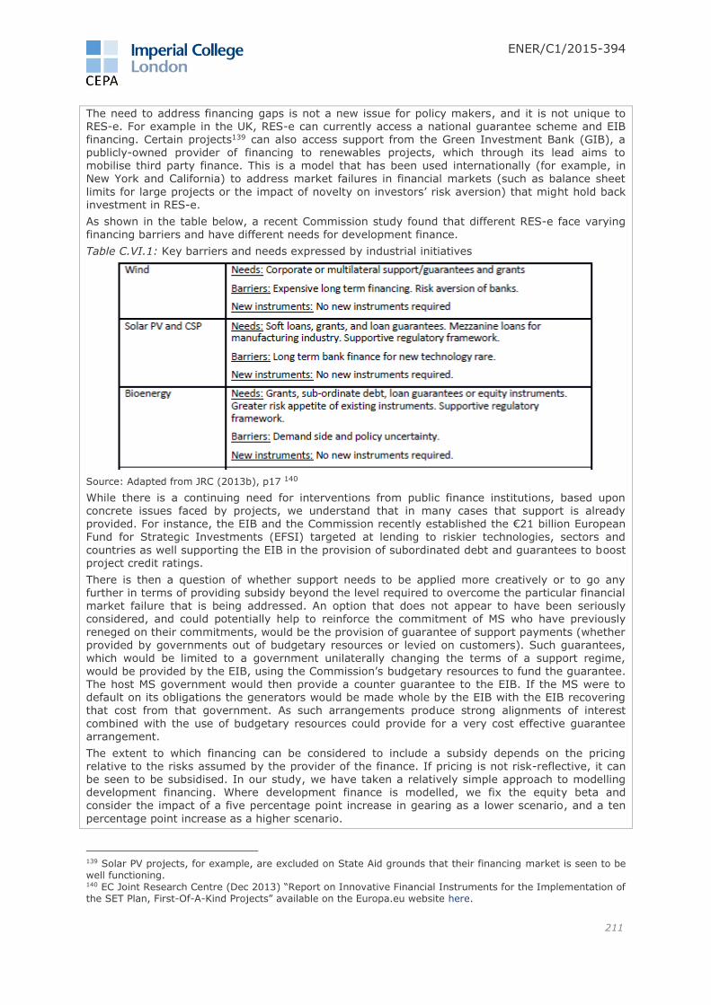
ENER/C1/2015-394

211

The need to address financing gaps is not a new issue for policy makers, and it is not unique to RES-e. For example in the UK, RES-e can currently access a national guarantee scheme and EIB financing. Certain projects139 can also access support from the Green Investment Bank (GIB), a publicly-owned provider of financing to renewables projects, which through its lead aims to mobilise third party finance. This is a model that has been used internationally (for example, in New York and California) to address market failures in financial markets (such as balance sheet

limits for large projects or the impact of novelty on investors’ risk aversion) that might hold back investment in RES-e.

As shown in the table below, a recent Commission study found that different RES-e face varying financing barriers and have different needs for development finance.

Table C.VI.1: Key barriers and needs expressed by industrial initiatives

Source: Adapted from JRC (2013b), p17 140

While there is a continuing need for interventions from public finance institutions, based upon concrete issues faced by projects, we understand that in many cases that support is already provided. For instance, the EIB and the Commission recently established the €21 billion European Fund for Strategic Investments (EFSI) targeted at lending to riskier technologies, sectors and

countries as well supporting the EIB in the provision of subordinated debt and guarantees to boost project credit ratings.

There is then a question of whether support needs to be applied more creatively or to go any further in terms of providing subsidy beyond the level required to overcome the particular financial market failure that is being addressed. An option that does not appear to have been seriously considered, and could potentially help to reinforce the commitment of MS who have previously

reneged on their commitments, would be the provision of guarantee of support payments (whether provided by governments out of budgetary resources or levied on customers). Such guarantees, which would be limited to a government unilaterally changing the terms of a support regime,

would be provided by the EIB, using the Commission’s budgetary resources to fund the guarantee. The host MS government would then provide a counter guarantee to the EIB. If the MS were to default on its obligations the generators would be made whole by the EIB with the EIB recovering that cost from that government. As such arrangements produce strong alignments of interest

combined with the use of budgetary resources could provide for a very cost effective guarantee arrangement.

The extent to which financing can be considered to include a subsidy depends on the pricing relative to the risks assumed by the provider of the finance. If pricing is not risk-reflective, it can be seen to be subsidised. In our study, we have taken a relatively simple approach to modelling development financing. Where development finance is modelled, we fix the equity beta and consider the impact of a five percentage point increase in gearing as a lower scenario, and a ten

percentage point increase as a higher scenario.

139 Solar PV projects, for example, are excluded on State Aid grounds that their financing market is seen to be well functioning. 140 EC Joint Research Centre (Dec 2013) “Report on Innovative Financial Instruments for the Implementation of the SET Plan, First-Of-A-Kind Projects” available on the Europa.eu website here.

http://publications.jrc.ec.europa.eu/repository/bitstream/JRC83675/ldna26058enn_002.pdf

ENER/C1/2015-394

212


This support mechanism would be a blended finance approach in which either commercial financiers or public development finance providers would use budgetary resources to soften the terms of finance provided. The justification for this softening of terms would be to prevent market-based pricing undermining the viability of projects. It would be used alongside primary support

mechanisms.

The focus of this intervention would therefore be on bridging the financing gap for projects, which are close to being investable/ bankable, but where specific problems means that they fail to attract sufficient finance, even with the support of a primary option. This would be targeted on less mature technologies with either higher costs and/or technology risk or; or where there is a lack of investor / lender confidence in government commitment to support

schemes.

Level of support

A variable subsidy element would be calibrated to bring down risk premia to affordable levels. Grants would be blended with:

Funded products such as subordinated loans will involve an interest rate subsidy, which will

reduce the risk reflectiveness of pricing relative to prices that the market would charge.

Credit or event specific guarantees (such as any issued in support of a MS payment commitments), in which the guarantee fee would not be fully risk reflective.

Eligibility

Only those projects which were close to bankability (assuming a primary support regime), but which needed additional assistance to attract finance.

Only where there is a demonstrable market or government failure (in the case of a given

MS’s previous history).


Allocation would be through an administrative process subject to State Aid clearance, if implemented on a national basis.

Administrator / Provider

Subsidies should be funded through a central budget, which has strict rules on eligibility, linked to

observed financing gaps either for specific technologies or at the country level. Including in the case of blending with commercial finance, grants would be administered by:

MS finance ministries (e.g., UK HM Treasury)

Multilateral development banks (e.g., EIB or EBRD)

National development banks (e.g., KfW)

Public entities established specifically to facilitate private investment into low carbon infrastructure (e.g., UK Green Investment Bank)


Unlike primary support options, the level of support cannot exceed the cost of finance

Credit analysis of projects by administrator’s staff ahead of providing loan

Duration

Grants would need to cover the life of the underlying instrument (although these can be front-loaded).


The subsidy can help leverage additional private finance flows for projects, which

are close to bankable.

Event specific guarantees could help government commitment to support regimes more credible.

Difficult to determine the appropriate level of grant support required (particularly

given greater difficulties in competing the subsidy).

Difficult to accurately target where it would be most additional: may not be sufficient

to attract commercial finance for more

ENER/C1/2015-394

213

Does not directly distort the wholesale market.

marginal projects, but greater danger of crowding out commercial finance where projects are less marginal.

ENER/C1/2015-394

214

Priority dispatch


Priority dispatch is a market access rule, which places an obligation on transmission system operators to schedule and dispatch RES-e generators ahead of all other types of generation. In

other words, priority dispatch artificially pushes some RES-e generators down the merit order, displacing other lower-cost conventional generators. The purpose of priority dispatch is to provide certainty to renewable generators that they will be able to sell electricity into the grid at all times (reducing volume risk), and to enable a more rapid integration of RES-e generators into the power system.

This means that priority generators will sometimes be selling electricity below their short-run

marginal cost (SRMC). For a rational generator, priority dispatch would not be a credible form of

support in-and-of itself, since routinely selling electricity below SRMC creates financial losses.141 Priority dispatch is therefore only effective if combined with other forms of operational support that increase the price received by the generator above the market clearing price.

Currently, priority dispatch is being combined with other forms of support (e.g., FITs & CfDs in UK) that make it profitable to sell electricity in the wholesale market at any price (even below marginal

cost). It is implemented for renewable electricity generators, but is relevant only for those with non-zero marginal costs, namely biomass.

The allocation of rights for priority dispatch has been purely administrative and is set out by Renewable Energy Directive, which states:

“Member States shall ensure that when dispatching electricity generating installations, transmission system operators shall give priority to generating installations using renewable energy sources” (2009/28/EC, paragraph 2(c))

However, it is also clearly set out in the legislation that in the event that renewable generators

participate in wholesale markets, the Directive does not require MS to provide support, or to make purchase obligations, for renewable electricity (2009/28/EC, paragraph 61). Overall, priority dispatch would seem to be targeted more at situations where renewable generators do not participate in wholesale markets, or where markets are underdeveloped.

The European Wind Energy Association (EWEA) recognises that the benefits of priority dispatch

(for wind) are more relevant when wind energy does not participate on equal footing to other types of generation in wholesale markets. They envision that priority dispatch should be phased out as markets continue to develop. They argue the following conditions should be met before removing priority dispatch:142

Existence of a fully functioning intraday and balancing market;

A satisfactory level of market transparency and proper market monitoring;

Priority dispatch for conventional generation and all other forms of non-RES-e power are

removed;

The requisite transmission and distribution infrastructure is in place;

Efficient system operation: best use of sophisticated forecasts and operational routines.

Efficiency implications:

While priority dispatch is designed to provide certainty to renewable generators, ensuring that they will be able to get their electricity to grid, it distorts the merit order and leads to a less efficient system overall.

Generators receiving priority dispatch (plus other forms of operational support) therefore do not respond efficiently to price signals in wholesale markets.

In an open letter to the Commission, a group of leading European economists argued that priority dispatch is a driving factors behind negative prices143 and that its short-term

distortive effects are greater even than a FIT (without priority dispatch).144

141 In some cases it may be rational to sell electricity below marginal costs if the cost of curtailing output (e.g., from shutting down) are greater than the lost revenue from selling below marginal cost. 142 EWEA (2014) 143 Though this is also attributable in part to the inflexibility of conventional generators. 144 Link here.

http://www.renewablesinternational.net/negative-prices-from-priority-for-renewables/150/537/81835/

ENER/C1/2015-394

215

o With evolving wholesale power markets, they argue that priority dispatch becomes less relevant and that good market design (without priority dispatch) is key to achieve good market outcomes, regardless of the form of operational support for renewables.

Other impacts/ Alternatives

Priority dispatch also indirectly addresses the failure of the ETS to produce sufficiently high carbon prices, which has led to conventional, carbon-producing, generators to be lower in the

merit order than they would have been with a well-functioning carbon market.

Alternative mechanisms to mimic the benefits of priority dispatch (in conjunction with other operational support) have been proposed that are less distortive to the merit order and result in overall efficiency savings compared to priority dispatch.

o Volume risk (e.g., risk of curtailment due to a transmission constraint) could be addressed by providing compensation to RES-e generators for the lost/potential (not

actual) output. In this situation, RES-e generators would not produce if they were not in merit, but would receive payments equal to their lost profits, had they been producing.

Overall, there seems to be consensus that priority dispatch has distortive effects on the wholesale markets by artificially re-configuring the merit order. However, it has been a useful tool to encourage integration of renewables into the European power system.


Eligibility of generators – currently only applicable to RES-e generators. Eligibility should be based on whether or not generators are able to participate on an equal footing in the wholesale markets. However, less distortive mechanisms that achieve equivalent outcomes are possible.

Length of eligibility – Only relevant if generators receive additional support so that the

price they receive is greater than SRMC. Therefore, length of eligibility should be linked to length of other support mechanisms.

Level of support

No direct payments made under a pure priority dispatch approach, as is being implemented currently in the EU.

Eligibility

Eligibility should be based on whether or not generators are able to participate on an equal footing in the wholesale markets. However, less distortive mechanisms that achieve equivalent outcomes are possible.


Administratively set by the Commission and enshrined in legislation, e.g., the Renewable Energy Directive (2009/28/EC).

Administrator

National implementation – priority dispatch is managed by transmission system operators that schedule and dispatch generators. This is only possible at the national level, or sub-national level in the case of multiple TSOs in a single MS (e.g., Germany or UK). However, national-only implementation could lead to distortions in the cross-border trade in electricity.

Regional/EU-wide implementation – not possible without regional cooperation of TSOs.


Priority dispatch, on its own, does not require any direct payments, and therefore has no material budgetary impacts.

Duration

Duration of priority dispatch should coincide with the duration of other support mechanisms that make priority dispatch financially viable for RES-e generators. It should also only persist if RES-e

generators are not able to participate on equal footing in wholesale markets.


Relatively simple to implement Lack of incentives for RES-e to respond to

ENER/C1/2015-394

216

wholesale market price

Causes inefficiencies in dispatch and deadweight loss

ENER/C1/2015-394

217

Exemption from balancing responsibility


The balancing mechanism is managed by the TSO, to ensure that supply and demand is continuously matched or balanced in real time. This entails the management of any residual

demand/supply disequilibrium unresolved by participants’ forward contracting activity. In a liberalised market, the market players have a responsibility to balance the system through the Balancing Responsible Parties (BRP). BRPs are legal entities that take on responsibility to compose a balanced portfolio. A BRP may represent one or more generators, suppliers and industrial consumers.

In the day-ahead market, the BRP’s portfolio must be balanced, meaning scheduled generation

equals forecasted demand. In the intraday market, the BRP can add intraday nominations to their

day-ahead nominations to correct their positions, following better output forecasts or unexpected outages. After clearing of the intraday market, the BRP’s portfolio can be in imbalance, which will be settled in the balancing market as explained below.

Market participants inform the TSO of their Final Physical Notifications (intended physical position) after gate closure, which informs the TSO of any actions it needs to engage to maintain the system in balance. The sum of the differences between market participants notified contractual positions

and their physical delivered or off-taken electricity indicates the level of energy imbalance on the system. The Net Imbalance Volume (NIV) is the net MWh value of all actions taken by the TSO in the settlement period. It is used to derive the main imbalance price in each period:

Positive NIV: corresponds to an upward regulation, meaning that the TSO has to increase injections in the grid or lower consumption in order to maintain balance;

Negative NIV: corresponds to a downward regulation, meaning that the TSO has to decrease injections in the grid or increase grid off-takes.

An imbalance price is usually calculated for each direction, these prices may however be the same,

allowing the possibility of both single pricing and dual pricing. Participants are exposed to their contractual disparity at a level determined by one of the two imbalance prices derived in each settlement period:

Market participants’ short position: if a participant has a shortage of supply vis-à-vis their nominations, they are charged a penalty which is no less than the weighted average

price for activated positive Balancing Energy for Frequency Restoration Reserves and Replacement Reserves;

Market participants’ long position: if a participant has a surplus of supply vis-à-vis their nominations, they get a payment, which is no more than the weighted average price for activated negative Balancing Energy for Frequency Restoration Reserves and Replacement Reserves.

Imbalance prices are intended to be reflective of the cost incurred by the TSO in its role of

managing system imbalance and should provide a disincentive for the market participants to aggravate the system imbalances.

For example, if a BRP’s position is long, the imbalance spread (imbalance price vs day-ahead price) should be negative if the system is long, to create a disincentive to produce when there is oversupply. Similarly, if the system is short, then the imbalance spread should be positive. Perverse incentives may exist when imbalance prices are constantly lower than the day-ahead market prices, meaning that BRPs are systematically rewarded for being short.

Under the State Aid Guidelines, support to RES-e generators is conditional on having a balancing responsibility. However, smaller RES-e installations (less than 3 MW for wind or below 500 kW for other sources) are exempt. In most MS with significant wind penetration (with the exception of Germany), wind is subject to balancing responsibilities, similar to conventional generators.

RES-e exposure to balancing responsibility usually results in a net cost, as prices tend to be low when they generate a surplus, and high when they are short.

Exempting RES-e from balancing responsibility weakens the incentives for RES-e to accurately forecast their output, which may result in a higher price volatility and a higher frequency of

negative prices.

We consider that the only rationale for justifying an exemption from balancing responsibility is if a RES-e generator does not have access to a well-functioning intraday and balancing market. If those markets are illiquid and/or imbalance prices not cost-reflective then the RES-e generator can

ENER/C1/2015-394

218

be exempt from balancing responsibility on a temporary basis.


Liquidity of national balancing market and cost-reflectivity of imbalance prices will determine

if the option is available in a country or region;

Temporary option that only addresses the market failure problem of national balancing markets that are inefficient and/or not cost-reflective.

Level of support

Determined by the BRP imbalance position during the settlement period and the system’s

position. The level of support corresponds to the avoided net imbalance costs that RES-e would pay to the TSOs if they had the financial responsibility of their position after gate closure.

Eligibility

Option only available for non-dispatchable energies that cannot control their generation and manage their imbalances.

Option available to RES-e generators in countries where national balancing and intraday markets are illiquid and where imbalance costs are not cost-reflective.


The allocation of this market preferential rule would be administratively decided at the national level, or at a regional level if regional balancing markets exist.

Administrator

National implementation: the option is implemented selectively by market in the event that

the national market is illiquid;

Regional/ EU implementation: only possible if a regional balancing market.


The primary means to control the budget for this support option is for policy makers to focus on creating liquidity in intraday markets ahead of balancing responsibility for RES-e generators.

Integration of cross-border intraday markets with continuous trading would also increase the accuracy of forecasts.

Duration

Limited; support should be progressively phased out when intraday and balancing markets become

efficient and imbalance prices cost-effective.


Increases RES-e participation in market without similar obligations as conventional generators

Distorts the day-ahead market as there are no incentives to forecast output correctly

ENER/C1/2015-394

219

Carbon contracting


The EU Emissions Trading System (ETS) is a major pillar of the EU climate policy and provides a platform for pricing carbon emissions through its cap-and-trade system. Its main goals are to

restrict the total level of emissions across Europe and to incentivise participants to invest in cleaner technology. Carbon contracting would provide eligible participants with a hedging product that mitigates the risk of low future ETS prices caused by a failure to follow through with the declared carbon policy.

The ETS covers power plants, energy intensive industries (e.g., steel manufacturing) and commercial aviation across the 28 EU MS and three non-EU countries (Iceland, Norway and

Liechtenstein). The ETS sets a limit (cap) on the overall level of CO2 emissions (and other

measurable greenhouse gases), and its design has evolved since its introduction in 2005. Currently, EU-wide emissions targets are set by the Commission and allocated to each participating country. Previously, ETS allowances (representing one tonne of CO2 each) were either allocated to companies for free or through a competitive auction. The default allocation method is now auctioning. After the auction/allocation process, participants can trade their allowances in secondary markets. ETS allowances may be traded internationally.

The allocation of ETS allowances has been organised into four ‘Phases’:

Phase 1 – most allowances were allocated freely. Over provision of allowances resulted in near zero prices.

Phase 2 – oversupply of credits combined with reduced output from the global recession led to low carbon prices (persistently below €10/ tonne in 2012).

Phase 3 – the current phase. Current ETS futures contracts for delivery in December 2016 trade at around €6/ tonne CO2.

Phase 4 – to be implemented from 2020, will reduce the emissions cap (and volume of

allowances) more rapidly which should increase carbon prices. This will be helped by mechanisms implemented in the course of Phase 3, such as the MSR.

It is widely recognised that oversupply of ETS allowances has led to the historically low ETS prices,145 which has prompted the development of the MSR and back-loading of allowances in Phase 3. This is because the supply of allowances is set administratively. Too many allowances

being disbursed meant that the total demand for allowances was less than supply, resulting in low carbon prices and dampened abatement efforts.

This is relevant for RES-e generators, since carbon prices filter through into wholesale electricity prices when conventional, carbon-emitting generators set prices. Therefore, with depressed ETS prices, RES-e generators have suffered due to lower wholesale prices than they otherwise would have. Since the ETS price is directly influenced by European policy (through the setting of the carbon cap), the failure of the ETS to price carbon accurately is directly related to policy. Our

analysis shows that by 2030 carbon costs could account for approximately 20% of the electricity price earned by RES-e generators, and therefore will represent component of the overall market

revenues.

Carbon contracts would provide eligible participants with a product that guarantees a certain level of carbon price (strike price), thereby providing a partial guarantee on one part of the wholesale price. The goal of such a product would be to address the failure of the ETS at producing relevant carbon prices by:

Making EU policy commitments (e.g., Phase 4) more credible – by being the counterparty to the contract, the EU would be at risk of paying out large sums of money for not delivering an efficient and effective ETS.

Providing downside protection to RES-e generators – contracts would provide insurance and increase certainty over one element of future wholesale prices.

As Newbery (2010) discusses,146 the risk associated with carbon prices is largely policy and

political, and impacts investors whose portfolios are much more focused on RES-e than investors with a more balanced portfolio that includes conventional generation. This is because conventional,

145 The Commission’s structural reform of the EU ETS is designed to deal with this surplus, and is described on

their website (link). 146 Newbery (2010)

http://ec.europa.eu/clima/policies/ets/reform/index_en.htm

ENER/C1/2015-394

220

price-setting generators are already hedged, to some extent, against carbon price volatility, since they can pass on their carbon costs to the consumers through wholesale electricity prices. The ability of carbon prices to drive low-carbon investments will depend on the predicted levels of ETS prices, as well as on investors' confidence that the prices will not fall below the point at which investments are unprofitable. Newbery describes the potential for carbon contracting to be set up as a contract for difference (CfD) on future carbon prices, either:

Two-sided – where generators would be entitled to receive the difference between the strike price and the spot price; or

One-sided – where generators receive the difference between the strike price and spot price only when the spot price falls below the strike price. This essentially sets a price floor. Another version of this would be to a put option on ETS prices.

To achieve efficient and market-driven pricing of contracts, the CfDs would be allocated through an

auction process. All parameters, apart from the price of the contract itself (e.g., contract length, volume of contracts), would be specified administratively.

The contract would specify a strike price, including a particular level of carbon price. We envision the contract as being purely a financial contract (i.e., not linked to generation), with contracts specified in terms of tonnes of CO2. Therefore, investors that are bidding for carbon contracts would need to calculate their exposure to carbon cost that are incorporate into wholesale electricity prices. Calculating the exposure to carbon is potentially complicated, which makes the

pricing of such a contract difficult, and thus may limit the interest of bidders. We consider that a one-sided CfD is likely to be more attractive, because under a two-sided CfD generators could be at a risk of paying (if ETS prices are higher than the strike price), even if they are not generating, given that the contract is not linked to generation.

In terms of efficiency, the question is whether such a product, underwritten by the EU, is filling a gap in the market. Currently, one is able to purchase futures contracts and options on ETS allowances, for example on the ICE exchange. While this does allow market participants to hedge

some of the volatility in carbon costs, it does not directly deal with the root cause of the risk—policy/political risk. The benefit of carbon contracts underwritten by the EU would be to increase the credibility of future EU policy, and to increase the certainty that investors may have regarding the ability of the EU to reform the ETS. It may be the case that providing even a small number of contracts, EU ETS policies may be seen to be more credible, and reduce the perceived risk even for investors who do not have a carbon contract. This, on the other hand, raises concerns of free-

riding by investors. In this case, investors who do not bid for carbon contracts benefit from the increased commitment to the declared policy provided by contracts bought by others.

This option would not be useful for RES-e support if investors also have access to other instruments that guarantee the wholesale price (e.g., a CfD or a FIT). However, it may be desirable to those RES-e generators if their existing support mechanisms are phased out, or to generators that are not eligible for other forms of support. Therefore, carbon contracting may be useful as a means of transitioning out of existing mechanisms.

In our study, we have taken a relatively simple approach to modelling carbon contracting. We

capture it through a reduction to the asset beta based on 20 percent of the difference between the value for Fixed FIP (with full wholesale risk) and FIT (with no wholesale risk), where 20 percent is our estimated share of wholesale market revenues related to the carbon price.


Strike price – the value of future ETS price that is guaranteed in the contract, determined administratively, and consistent with carbon policy.

Length of contract – determined administratively. Longer-term contracts would make them more useful as a hedge against long-term policy risk.

Number of contracts – the number of contracts auctioned should be limited in order to create scarcity and reasonable price signals. This total number of contracts auctioned would

be determined administratively, and should be sufficient to support all new RES-e installations that are required to meet the RES-e target (which is specified in terms of MWh).

Level of support

We would envision the contract being a one-sided CfD, providing protection against downside risk and allowing the owner of the CfD to capture upside benefits.

The contract is similar to traditional insurance, protecting against potentially unlikely

ENER/C1/2015-394

221

downside events. The downside event, in this case, is a weak regulatory commitment to delivering sufficiently high ETS prices. The attractiveness of the contract is, therefore, influenced by how strong the commitment made in the contract is, which is reflected in level of the strike price and length of the contract.

Carbon contracts are potentially difficult for investors to value, since the exposure to ETS prices, which form part of the wholesale electricity price, depends on the type of technology

setting prices at each hour of the day during the life of the plant.

Eligibility

Eligibility to participate in carbon contracts would be open to all types of generators and other interested parties. This includes, for example, DSR, industry and other businesses that may

invest in energy efficiency products. Carbon contracting should encourage investment in low-carbon technologies. Different participants are expected to value these contracts, including:

o RES-e generators that would have an incentive to bid for carbon contracts that lock-in high ETS prices and provide greater certainty over an element of wholesale revenues.

o DSR and industry can use carbon contracts to lock-in efficiency benefits of energy efficiency investments. Therefore, they are expected to value such contracts.

While conventional carbon-emitting generators may prefer lower carbon prices, they are

already hedged to some extent, as they are able to pass on increased carbon costs to consumers whenever they are in merit. They could use carbon contracts to lock-in benefits from investments in low carbon technologies such as CCS, as well as energy efficiency investments. Therefore, conventional generators may value such contracts, but probably to a lesser extent, than other participants.


The allocation of carbon contracts would be through a competitive auction. Contracts of different

lengths could also be auctioned in a given year, but longer-term contracts are likely to be more useful as a hedge against policy risk.

Administrator

European implementation – the scheme would be administered by the Commission, including the setting of key parameters. Newbery (2010) also advocates that price stability should be pursued at the EU level.

National implementation could be feasible, but is less likely to be effective, since MS do not directly control ETS policy. In this case, the hedge against policy risk would be less effective,

therefore we did not consider national implementation as part of our assessment.


The primary means of budget control would be the ability of the EU to deliver ETS prices that are at least as high as those contained in the carbon contract.

Also, the level at which the strike price is set, the volume of contracts auctioned, and whether

or not the CfD contract is one-sided or two-sided will influence the budget impact.

o One-sided contracts could potentially be more expensive since generators would keep any upside benefits. However, depending on the strike price, they may be valued higher, and generate more auction proceeds.

Duration

The duration of the carbon contracting programme should coincide with the length of the ETS Phase in which ETS contracts are relevant, but could also span across different Phases of the ETS to provide longer-term policy commitment.

We do not consider that the 10-year maximum duration for RES-e support schemes, as described under State Aid Guidelines (3.3.1. (121)) would apply, as carbon contracts would be open to all generation technologies, industry and DSR.


Addresses main risk (policy) associated with ETS

Increases credibility of policy and reduces

Pricing potentially complicated (since calculating individual generator’s exposure to carbon, through wholesale price is

ENER/C1/2015-394

222

volatility of ETS revenues

Encourages investment in low-carbon technologies

difficult)

Potential for free-riding by RES-e generators (i.e., generators benefit from increased policy credibility without buying the product)

Limited interest from investors is likely

ENER/C1/2015-394

223

ANNEX E Qualitative assessment of relative risk As part of our analysis of discount rates, we completed a qualitative relative risk

exercise, allowing us to adopt an approach capable of attributing quantitative

adjustments to the cost of capital for combinations of technologies and support schemes

where comparator values were not available. This annex provides a summary of our

findings.

In this analysis, we adopted a structured approach to compare the risk exposure of RES-

e technologies with those of a conventional generator, and to compare the risk exposure

of the primary support options considered in this report with those under a FIT.

To allow us to use this qualitative analysis to attribute quantitative values to particular

technologies and support schemes, we conducted our risk analysis for technologies and

support schemes along three dimensions:

1. cost of debt;

2. CAPM asset beta; and

3. project-specific risk

We present our findings for each dimension in turn, noting how these how each was

used in our discount rate analysis.

Cost of debt

To consider how relative risk might affect the cost of debt, we assumed a fixed credit

rating for generators (approximately AA) and used our qualitative analysis to determine

the maximum gearing level at which a generator might be able to achieve that cost of

debt. Therefore, to consider how relative risk might affect the level of gearing a debt

investor might permit in a RES-e project, we analysed technologies and support schemes

in a framework based on Moody’s ratings methodology for power generation. Within this

framework, we considered risks in three categories:

1. Predictability of cashflows: risks affecting the quality and diversity of

cashflows, including conditions for contractual payments. This category included

capex risk, opex risk, fuel risk (biomass only), revenue risk (P90 confidence

level), and counterparty/payment risk once operational.

2. Regulatory support: risks related to the support provided at the national,

regional or EU level (for support schemes only).

3. Technology and Operating risks: risks related to renewable technology

compared to conventional energy, including changes in maturity of technology

over time and size of construction programme.147

Tables E.1 and E.2 below present our findings from relative risk analysis on the cost of

debt dimension by technology and by support scheme. In each case, an upward arrow

was assigned to cases considered higher risk than the reference point. Downward arrows

were assigned to note lower risk. The output of the analysis was a set of overall relative

risk judgements, which in the case of technologies were allowed to vary over time as

technologies mature.

As can be seen in the tables, we found Solar PV to be the least risky technology from a

debt investor perspective, followed by onshore wind; we found geothermal and tidal

range to be the riskiest. In terms of support schemes, we found grants to be the most

favourable for debt investors; we found Fixed FIP and RO schemes to be the riskiest.

147 The size of a project may affect risks due to complexity. The scalability of a plant can on the other hand reduce risks related to the size of a construction programme.

ENER/C1/2015-394

224

We used the summary findings from this relative risk analysis as an ordinal restriction on

the gearing parameter values used in our discount rates analysis such that, for example,

a solar PV project with a grant would have a higher gearing level in our discount rate

calculations than a geothermal plant with a Fixed FIP. The precise quantitative margin

between each case was determined through calibration against external sources.

Table E.1: Relative risk analysis on the cost of debt dimension for RES-e technologies

Table E.2: Relative risk analysis on the cost of debt dimension for support options

CAPM approach

Given its forward-looking nature, estimation of the cost of equity is more challenging

than the cost of debt. Therefore, to adjust the cost of equity for technology and support

schemes, we captured relative risk differences through the asset beta used in our CAPM

framework.

The key difference between the CAPM approach and the cost of debt dimension is that

for equity investors, certain risks may not affect their returns so long as they can be

diversified away across a portfolio. Therefore, while in the analysis of relative risk in this

dimension, we considered capex risk, opex risk and fuel risk (biomass only) in a manner

similar to the cost of debt dimension. We additionally considered financing risk, inflation

risk, and split revenue risk into wholesale risk and volume risk (P50 level of confidence).

COST OF DEBT Solar PV Onshore wind

Offshore wind

Biomass Hydro ROR Hydro Reservoir


Factor 1: Predictability of cashflows

Internal - Cost risks

Capex risk =

Opex risk =/

Fuel risk =

Internal - Revenue risk

Volume risk (P90 assumption) =

Price risk = = = = = = = =

Counterparty/ payment risk = = = = = = = =

Factor 2: Regulatory support

Stability and predictability

Factor 3: Tech and Operating Risks

Maturity of technology 2016 = = =/ = =

Maturity of technology 2020 = = =/ =/ = =

Maturity of technology 2025 = = = =/ = =

Maturity of techno 2030 = = = = = = /

Maturity of techno 2040 = = = = = =

Maturity of techno 2050 = = = = = = /

Size of construction programme =/

OVERALL (2016) = =/ =/

OVERALL (2020) = =/ =/

OVERALL (2025) = =/ =/ =/

OVERALL (2030) = =/ = =/ /

OVERALL (2040) = =/ = =/

OVERALL (2050) = =/ = =/ /

COST OF DEBT Floating FIP Fixed FIP Quota scheme Grant

Factor 1: Predictability of cashflows

Internal - Cost risks

Capex risk = = =

Opex risk = = = =

Fuel risk

Internal - Revenue risk

Revenue risk =/

Counterparty/ payment risk =/ =/ =/

Factor 2: Regulatory support

Stability and predictability = =

Factor 3: Tech and Operating Risks

Maturity of technology

Size of construction programme

OVERALL =/

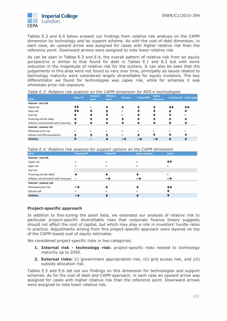
ENER/C1/2015-394

225

Tables E.3 and E.4 below present our findings from relative risk analysis on the CAPM

dimension by technology and by support scheme. As with the cost of debt dimension, in

each case, an upward arrow was assigned for cases with higher relative risk than the

reference point. Downward arrows were assigned to note lower relative risk.

As can be seen in Tables E.3 and E.4, the overall pattern of relative risk from an equity

perspective is similar to that found for debt in Tables E.1 and E.2 but with some

reduction in the magnitude of relative risk for the outliers. It can also be seen that the

judgements in this area were not found to vary over time, principally as issues related to

technology maturity were considered largely diversifiable for equity investors. The key

differentiator we found for technologies was capex risk, while for schemes it was

wholesale price risk exposure.

Table E.3: Relative risk analysis on the CAPM dimension for RES-e technologies

Table E.4: Relative risk analysis for support options on the CAPM dimension

Project-specific approach

In addition to fine-tuning the asset beta, we extended our analysis of relative risk to

particular project-specific diversifiable risks that corporate finance theory suggests

should not affect the cost of capital, but which may play a role in investors’ hurdle rates

in practice. Adjustments arising from this project-specific approach were layered on top

of the CAPM-based cost of equity estimates.

We considered project-specific risks in two categories:

1. Internal risk - technology risk: project-specific risks related to technology

maturity up to 2050.

2. External risks: (i) government appropriation risk, (ii) grid access risk, and (iii)

subsidy allocation risk.

Tables E.5 and E.6 set out our findings on this dimension for technologies and support

schemes. As for the cost of debt and CAPM approach, in each case an upward arrow was

assigned for cases with higher relative risk than the reference point. Downward arrows

were assigned to note lower relative risk.

BETA Solar PV

Onshore wind

Offshore wind



Internal - cost risk

Capex risk =

Opex risk =

Fuel risk = =

Financing risk (for debt)

Inflation risk (mismatch with revenues)

Internal - revenue risk

Wholesale price risk = = = = = = = =

Volume risk (P50 assumption) =

OVERALL = =/ =/ =/

BETA Floating FIP Fixed FIP Quota scheme Grant

Internal - cost risk

Capex risk = = =

Opex risk = = = =

Fuel risk

Financing risk (for debt) =

Inflation risk (mismatch with revenues) = =/ =/ =/

Internal - revenue risk

Wholesale price risk =/

Volume risk = = =

OVERALL =/

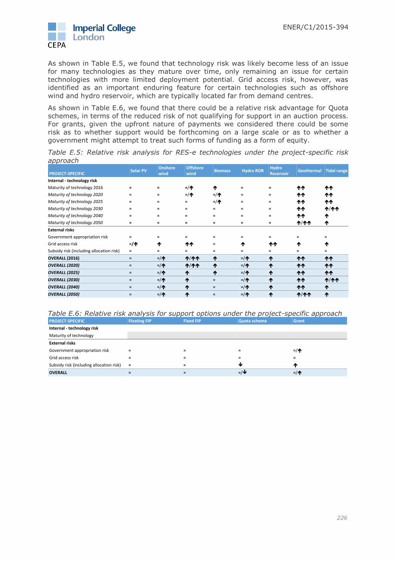
ENER/C1/2015-394

226

As shown in Table E.5, we found that technology risk was likely become less of an issue

for many technologies as they mature over time, only remaining an issue for certain

technologies with more limited deployment potential. Grid access risk, however, was

identified as an important enduring feature for certain technologies such as offshore

wind and hydro reservoir, which are typically located far from demand centres.

As shown in Table E.6, we found that there could be a relative risk advantage for Quota

schemes, in terms of the reduced risk of not qualifying for support in an auction process.

For grants, given the upfront nature of payments we considered there could be some

risk as to whether support would be forthcoming on a large scale or as to whether a

government might attempt to treat such forms of funding as a form of equity.

Table E.5: Relative risk analysis for RES-e technologies under the project-specific risk

approach

Table E.6: Relative risk analysis for support options under the project-specific approach

PROJECT-SPECIFIC Solar PV

Onshore wind

Offshore wind



Internal - technology risk

Maturity of technology 2016 = = =/ = =

Maturity of technology 2020 = = =/ =/ = =

Maturity of technology 2025 = = = =/ = =

Maturity of technology 2030 = = = = = = /

Maturity of technology 2040 = = = = = =

Maturity of technology 2050 = = = = = = /

External risks

Government appropriation risk = = = = = = = =

Grid access risk =/ =

Subsidy risk (including allocation risk) = = = = = = = =

OVERALL (2016) = =/ / =/

OVERALL (2020) = =/ / =/

OVERALL (2025) = =/ =/

OVERALL (2030) = =/ = =/ /

OVERALL (2040) = =/ = =/

OVERALL (2050) = =/ = =/ /

PROJECT-SPECIFIC Floating FIP Fixed FIP Quota scheme Grant

Internal - technology risk

Maturity of technology

External risks

Government appropriation risk = = = =/

Grid access risk = = = =

Subsidy risk (including allocation risk) = =

OVERALL = = =/ =/

ENER/C1/2015-394

227

ANNEX F Demand side response and energy storage methodology The purpose of this Annex is to describe how we: (1) developed demand side response

and storage capacity estimates; and (2) incorporated these estimates into our energy

market simulations.

It is well understood that as the proportion of variable generation from renewables in the

generation mix increases, so does the need for flexibility in an electricity network as

supply and demand for electricity must match at all times. Indeed, this is apparent in the

Commission’s new market design consultation that has a vision to ‘…fully integrate all

market players – including flexible demand, energy service providers and renewables.’148

IRENA (2015) describes how four interrelated sources provide system flexibility:149

flexible dispatchable generators (primarily, gas-fired—OCGTs and CCGTs,

and hydro generators, including pumped storage);

interconnection (i.e., ‘leaning’ on neighbouring systems to manage variable

generation);

demand side response; and

new energy storage (both conventional, e.g., pumped storage, as well as

new storage devices, e.g., batteries).

The most important aspect of the flexibility challenge is that newly constructed,

conventional flexible capacity is unlikely to replace the decline in existing, flexible

conventional capacity. Although interconnection capacity is likely to grow between MS,

those increases may not be sufficient to meet flexibility needs of many MS in the future.

Thus, we expect that, in order to meet their flexibility challenge, many MS will tap into

their DSR potential and/or develop new energy storage capacity.

Graphically, the availability of different sources of system flexibility, and their possible

evolution over time, is illustrated in a stylized example in Figure F.1 below.

Figure F.1: The role of flexibility in the context of variable generation

Source: CEPA

While most MS will face the flexibility challenge to accommodate high(er) levels of

renewable generation, they will have varying degrees of ability to deploy these sources

of flexibility. For example, some MS may be weakly interconnected with other markets

and constructing new interconnectors may not be cost-effective. Similarly, the ability of

some MS to construct new pumped storage plants may be limited by their geography.

148 https://ec.europa.eu/energy/en/consultations/public-consultation-new-energy-market-design 149 IRENA (2015)

Flexibility

RES-e penetration

Existing

flexibility

DSM

Storage

Interconnection

Dispatchable

supply

Flexibility need

https://ec.europa.eu/energy/en/consultations/public-consultation-new-energy-market-design

ENER/C1/2015-394

228

Our working assumption was that each MS will find the least-cost mix of meeting the

flexibility challenge best suited to its unique circumstances. Thus, each of the flexibility

sources shown above will be competing against one another in terms of cost-

effectiveness. In the context of the Commission’s new market design in which market

participants, including flexible demand, are integrated and have access to wholesale

markets, the lowest-cost source of flexibility should prevail. Ability to provide system

flexibility is just one feature of conventional generators (i.e., in addition to generating

electricity); thus:

In developing our DSR assumptions we took PRIMES projections of flexible

capacity, from the EUCO27 scenario as given.

Similarly, EU targets largely drive increases in interconnection capacity. We assume that

no significant interconnection will be built once targets are met (though WeSIM

endogenously adds capacity if it is efficient to do so), because such capacity is relatively

expensive, although new interconnection has desirable roles beyond flexibility (e.g.,

security of supply).

Therefore, we took ENTSO-E’s interconnection projections between MS pairs as

given. In a number of MS, especially in continental Europe, interconnection is

relatively developed, and thus served as a significant source of system flexibility.

Any flexibility need not met by conventional generation and interconnection will have to

be met by DSR and new energy storage. Presently, large-scale storage technologies are

relatively expensive, and in some cases limited by geography (e.g., pumped storage). In

contrast, DSR is a relatively untapped resource in Europe that offers a potentially

attractive and cost-effective solution (compared to other capital-intensive solutions) to

fulfilling the flexibility needs of MS, and forms part of the overall package of flexibility.

As noted below, experience of some markets suggests that significant DSR penetration

can realistically be achieved, and much of that DSR can be provided at a relatively low

cost.

Demand Side Response

DSR in this section refers to changes in consumption patterns can help provide system

flexibility. In simple terms, DSR can be defined as a change in the level and pattern of

electricity demand in response to price or other incentives. In the context of the

Commission’s new market design, we assume that the DSR will primarily occur in

response to market prices, and that system flexibility needs will be appropriately

reflected in those prices.

DSR can generally come in several different forms:

Load reduction. This represents a permanent reduction in load (i.e., load

that is curtailed and not shifted to another time of day). This effect will

come from different types of end use demand. For example, a large

supermarket may dim their lights in response to high prices, or an industrial

process may be suspended temporarily/ be switched over to backup

generators during periods of high prices.

Load shifting. This represents a temporal shift in load (i.e., a reduction in

one period and an increase during another period), which can occur across

different demand types. For domestic load, an example would be pre-

cooling a building before higher-priced hours, or using appliances only at

times with low prices.

Load increase. For example, power plants have minimum sustainable

generation levels, and at night this is often a binding constraint. Some loads

(e.g., street lighting) may be used to manage this constraint. Growing wind

penetration will make this problem worse on windy nights—however, since

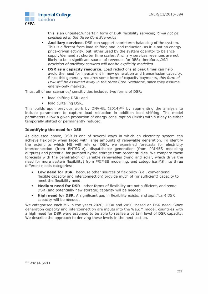
ENER/C1/2015-394

229

this is an untested/uncertain form of DSR flexibility services; it will not be

considered in the three Core Scenarios.

Ancillary services. DSR can support short-term balancing of the system.

This is different from load shifting and load reduction, as it is not an energy

price-driven activity, but rather used by the system operator to balance

supply/demand at shorter time scales. Ancillary services revenues are not

likely to be a significant source of revenues for RES; therefore, DSR

provision of ancillary services will not be explicitly modelled.

DSR as a capacity resource. Load reductions at peak times can help

avoid the need for investment in new generation and transmission capacity.

Since this generally requires some form of capacity payments, this form of

DSR will be assumed away in the three Core Scenarios, since they assume

energy-only markets.

Thus, all of our scenarios/ sensitivities included two forms of DSR:

load shifting DSR; and

load curtailing DSR.

This builds upon previous work by DNV-GL (2014)150 by augmenting the analysis to

include parameters to capture load reduction in addition load shifting. The model

parameters allow a given proportion of energy consumption (MWh) within a day to either

temporally shifted or permanently reduced.

Identifying the need for DSR

As discussed above, DSR is one of several ways in which an electricity system can

achieve flexibility when faced with large amounts of renewable generation. To identify

the extent to which MS will rely on DSR, we examined forecasts for electricity

interconnection (from ENTSO-e), dispatchable generation (from PRIMES modelling

outputs) and potential for pumped hydro storage from recent studies. We compare these

forecasts with the penetration of variable renewables (wind and solar, which drive the

need for more system flexibility) from PRIMES modelling, and categorise MS into three

different needs categories:

Low need for DSR—because other sources of flexibility (i.e., conventional

flexible capacity and interconnection) provide much of (or sufficient) capacity to

meet the flexibility need.

Medium need for DSR—other forms of flexibility are not sufficient, and some

DSR (and potentially new storage) capacity will be needed

High need for DSR. A significant gap in flexibility exists, and significant DSR

capacity will be needed.

We categorised each MS in the years 2020, 2030 and 2050, based on DSR need. Since

generation capacity and interconnection are inputs into the WeSIM model, countries with

a high need for DSR were assumed to be able to realise a certain level of DSR capacity.

We describe the approach to deriving these levels in the next section.

150 DNV-GL (2014

ENER/C1/2015-394

230

Figure F.2: Stylised representation of identified need for DSR

Source: CEPA

Quantifying total DSR

For each MS, the penetration of DSR was built up based on the notion of ‘achievable

potential’, which represents the maximum amount of load shifting/curtailment that can

be realised.

A large number of studies have been carried out that examine the amount of peak

shaving that can be achieved through DSR. CEPA (2014) conducted a literature review of

the potential impact of DSR and found that estimates of potential peak clipping range

from 10-20%. These findings are supported by the fact that DSR in some markets in the

USA (e.g., PJM) has already grown to 10% of peak demand. A summary of some of the

results is shown in Table F.1 below.

Table F.1: Summary of DSR potential studies

Study Estimated peak

load reduction Notes

Empower

Demand

(2011)151

10-13% Based on 15 real-time pricing (RTP) trials (3 in Europe and

12 in the USA). Did not differentiate by peak/off-peak ratio.

Faruqui

(2013)152 15-25%

Based on a meta-analysis of studies that show the impact

based on the peak/off-peak price ratio. The range is

presented for the main clustering of price ratios from

studies, which is around 8 (peak/off-peak).

EC (2014b)153 1-10%

Relates to peak shifting and includes impact from greater

awareness of consumption. This range is based on the

results of EC SWD (2014) 188 & 189, which focussed on the

roll-out of smart metering. The percentage represents

percent of total consumption, and results varied by country.

Also considered the time required to roll-out smart metering

programmes, which by country and level of penetration, but

were on average 6 years.

EWI (2012)154 10% Potential size of DSR resource by 2050. The 10% is intended

to be achievable based on a potential level of 18%. The

151 Empower Demand (2011) 152 Faruqui (2013) 153 EC (2014b) 154 EWI (2012)

Flexibility

without

DSR

RES-e penetration

Low DSR

need

Medium DSR

need

High DSR

need

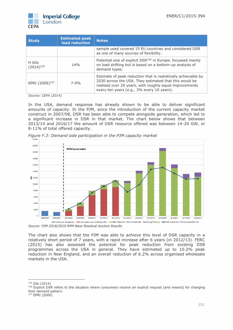
ENER/C1/2015-394

231

Study Estimated peak

load reduction Notes

sample used covered 15 EU countries and considered DSR

as one of many sources of flexibility.

H Gils

(2014)155 14%

Potential size of explicit DSR156 in Europe, focussed mainly

on load shifting but is based on a bottom-up analysis of

demand types.

EPRI (2009)157 7-9%

Estimate of peak reduction that is realistically achievable by

2030 across the USA. They estimated that this would be

realised over 20 years, with roughly equal improvements

every ten years (e.g., 3% every 10 years).

Source: CEPA (2014)

In the USA, demand response has already shown to be able to deliver significant

amounts of capacity. In the PJM, since the introduction of the current capacity market

construct in 2007/08, DSR has been able to compete alongside generation, which led to

a significant increase in DSR in that market. The chart below shows that between

2013/14 and 2016/17 the amount of DSR resource offered was between 14-20 GW, or

8-11% of total offered capacity.

Figure F.3: Demand side participation in the PJM capacity market

Source: PJM 2018/2019 RPM Base Residual Auction Results

The chart also shows that the PJM was able to achieve this level of DSR capacity in a

relatively short period of 7 years, with a rapid increase after 6 years (in 2012/13). FERC

(2015) has also assessed the potential for peak reduction from existing DSR

programmes across the USA in general. They have estimated up to 10.2% peak

reduction in New England, and an overall reduction of 6.2% across organised wholesale

markets in the USA.

155 Gils (2014) 156 Explicit DSR refers to the situation where consumers receive an explicit request (and reward) for changing

their demand pattern. 157 EPRI (2009)

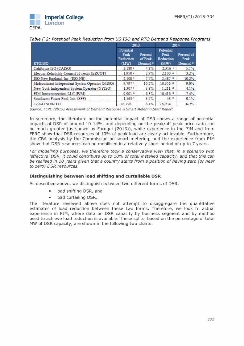
ENER/C1/2015-394

232

Table F.2: Potential Peak Reduction from US ISO and RTO Demand Response Programs

Source: FERC (2015) Assessment of Demand Response & Smart Metering Staff Report

In summary, the literature on the potential impact of DSR shows a range of potential

impacts of DSR of around 10-14%, and depending on the peak/off-peak price ratio can

be much greater (as shown by Faruqui (2013)), while experience in the PJM and from

FERC show that DSR resources of 10% of peak load are clearly achievable. Furthermore,

the CBA analysis by the Commission on smart metering, and the experience from PJM

show that DSR resources can be mobilised in a relatively short period of up to 7 years.

For modelling purposes, we therefore took a conservative view that, in a scenario with

‘effective’ DSR, it could contribute up to 10% of total installed capacity, and that this can

be realised in 10 years given that a country starts from a position of having zero (or near

to zero) DSR resources.

Distinguishing between load shifting and curtailable DSR

As described above, we distinguish between two different forms of DSR:

load shifting DSR, and

load curtailing DSR.

The literature reviewed above does not attempt to disaggregate the quantitative

estimates of load reduction between these two forms. Therefore, we look to actual

experience in PJM, where data on DSR capacity by business segment and by method

used to achieve load reduction is available. These splits, based on the percentage of total

MW of DSR capacity, are shown in the following two charts.

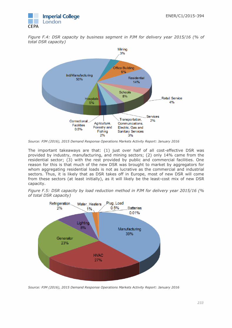
ENER/C1/2015-394

233

Figure F.4: DSR capacity by business segment in PJM for delivery year 2015/16 (% of

total DSR capacity)

Source: PJM (2016), 2015 Demand Response Operations Markets Activity Report: January 2016

The important takeaways are that: (1) just over half of all cost-effective DSR was

provided by industry, manufacturing, and mining sectors; (2) only 14% came from the

residential sector; (3) with the rest provided by public and commercial facilities. One

reason for this is that much of the new DSR was brought to market by aggregators for

whom aggregating residential loads is not as lucrative as the commercial and industrial

sectors. Thus, it is likely that as DSR takes off in Europe, most of new DSR will come

from these sectors (at least initially), as it will likely be the least-cost mix of new DSR

capacity.

Figure F.5: DSR capacity by load reduction method in PJM for delivery year 2015/16 (%

of total DSR capacity)


ENER/C1/2015-394

234

In Figure F.5, we see the methods used to achieve the level of DSR capacity in the PJM.

Broadly speaking, these will cover both shiftable and curtailable load, and will span the

different business segments covered in Figure F.4. Based on this information, we have

done a qualitative assessment of potential for the various types of DSR resources in the

PJM to provide shiftable/curtailable capacity (refer to F.10). Based on this, we

constructed an assumption of the percentage of total achievable DSR potential that

constitutes shiftable vs. curtailable load.

Table F.3: Assumed shiftable and curtailable DSR proportions

% of total achievable DSR potential

Shiftable potential 40%

Curtailable potential 60%

As a cross-check to this assumption we also conducted a high-level analysis of the

demand mix for each MS and made a qualitative judgement as to whether they will be

able to reach the achievable potential of DSR. For example, evidence from the PJM

suggests that a large proportion of achievable DSR can come from

Industry/Manufacturing (see Figure F.4). Some countries, such as Cyprus, have little

manufacturing, in which case it is less likely that they will be able to realise the

achievable potential of DSR. In such a case, we reduced the achievable level of DSR in

that MS by 50%. We based our assessment of the level of manufacturing/industry on

Eurostat’s published energy balances for 2014.

Enabling policy cross-check

In practice the penetration of DSR will vary by MS and will be either

hindered/encouraged by national policies. The main enabling policies at the European

level are the RES Directive (2009/28CE) and Energy Efficiency Directive (2012/27/EU),

but there still exists some disparity in the adoption of enabling policies at the national

level. The rate at which countries will be able to realise DSR is also dependent on the

level of need (i.e., the level of DSR we assume will be realised). While we consider that it

is appropriate to assume that enabling policies will be in place in the future to allow

countries to have sufficient DSR, we use the current state of play as an indicator of

whether this is a realistic expectation in the near future (e.g., within the next decade).

This led, in some cases, to adjusting the year in which the full level DSR needed is

realised.

The SEDC (2015)158 assessed the current state of play for DSR policies across 16 MS in

2015, focussing primarily on explicit DSR defined as “…the control of aggregated

changes in load are traded in electricity markets, providing comparable services to

supply side resources, and receiving the same prices for those services.” They based

their analysis on four criteria:

1. Enabling consumer participation and aggregation.

2. Appropriate programme requirements.

3. Fair and standardised measurement and verification requirements.

4. Equitable payment and risk structures.

They found that Ireland, UK, France, Switzerland and Finland have commercially active

explicit DSR already, while other countries are less well developed. This is shown in the

map below.

158 SEDC (2015)

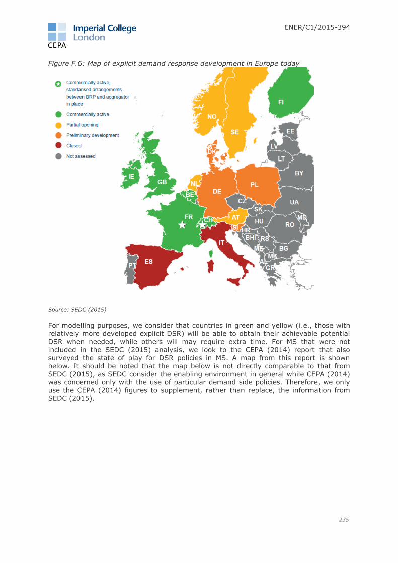
ENER/C1/2015-394

235

Figure F.6: Map of explicit demand response development in Europe today

Source: SEDC (2015)

For modelling purposes, we consider that countries in green and yellow (i.e., those with

relatively more developed explicit DSR) will be able to obtain their achievable potential

DSR when needed, while others will may require extra time. For MS that were not

included in the SEDC (2015) analysis, we look to the CEPA (2014) report that also

surveyed the state of play for DSR policies in MS. A map from this report is shown

below. It should be noted that the map below is not directly comparable to that from

SEDC (2015), as SEDC consider the enabling environment in general while CEPA (2014)

was concerned only with the use of particular demand side policies. Therefore, we only

use the CEPA (2014) figures to supplement, rather than replace, the information from

SEDC (2015).

ENER/C1/2015-394

236

Figure F.7: Time-based electricity supply tariffs by customer group

Source: CEPA (2014), The Potential Benefits and State of Play in the European Union.

Modelling load shifting DSR

The WeSIM model uses a single parameter for modelling load shifting DSR: the

percentage of daily peak demand that is shiftable. The general logic is shown in the

stylised figure below.

Figure F.8: Stylised representation of demand shifting

For the modelled scenarios, we base this percentage on our notion of achievable

potential, which has been split by shiftable/curtailable DSR. Each MS has also been

placed in a category for their need for DSR, which we use to scale the achievable

potential.

MS with a high DSR need will get the full achievable potential

MS with medium DSR need will het half of the achievable potential

MS with low DSR need will get a quarter of the achievable potential

With consideration to both the rate at which achievable potential can be realised, the

level of DSR needed and the enabling policies of MS, we also set a year in which we

Malta

Cyprus

Malta

Cyprus

Demand

Time

Residential customers

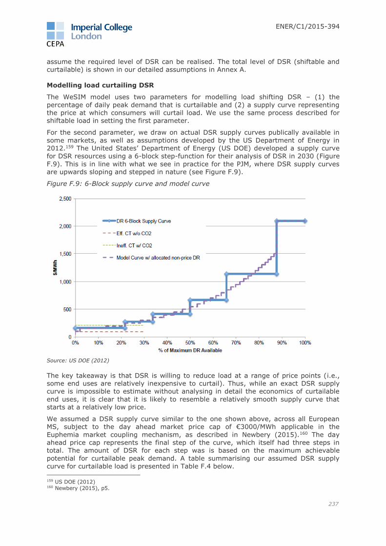
ENER/C1/2015-394

237

assume the required level of DSR can be realised. The total level of DSR (shiftable and

curtailable) is shown in our detailed assumptions in Annex A.

Modelling load curtailing DSR

The WeSIM model uses two parameters for modelling load shifting DSR – (1) the

percentage of daily peak demand that is curtailable and (2) a supply curve representing

the price at which consumers will curtail load. We use the same process described for

shiftable load in setting the first parameter.

For the second parameter, we draw on actual DSR supply curves publically available in

some markets, as well as assumptions developed by the US Department of Energy in

2012.159 The United States’ Department of Energy (US DOE) developed a supply curve

for DSR resources using a 6-block step-function for their analysis of DSR in 2030 (Figure

F.9). This is in line with what we see in practice for the PJM, where DSR supply curves

are upwards sloping and stepped in nature (see Figure F.9).

Figure F.9: 6-Block supply curve and model curve

Source: US DOE (2012)

The key takeaway is that DSR is willing to reduce load at a range of price points (i.e.,

some end uses are relatively inexpensive to curtail). Thus, while an exact DSR supply

curve is impossible to estimate without analysing in detail the economics of curtailable

end uses, it is clear that it is likely to resemble a relatively smooth supply curve that

starts at a relatively low price.

We assumed a DSR supply curve similar to the one shown above, across all European

MS, subject to the day ahead market price cap of €3000/MWh applicable in the

Euphemia market coupling mechanism, as described in Newbery (2015).160 The day

ahead price cap represents the final step of the curve, which itself had three steps in

total. The amount of DSR for each step was is based on the maximum achievable

potential for curtailable peak demand. A table summarising our assumed DSR supply

curve for curtailable load is presented in Table F.4 below.

159 US DOE (2012) 160 Newbery (2015), p5.

ENER/C1/2015-394

238

Table F.4: Curtailable load supply curve

% of maximum curtailable peak load Price (€/MWh)

0-33% 250

34-66% 1500

>66% 3000

Source: CEPA

The total level of DSR (shiftable and curtailable) is shown in our detailed assumptions in

Annex A.

Non-conventional storage

Given the total amount of flexibility provided by DSR, interconnection and dispatchable

generation, there may still be a need for additional flexibility in MS. We assume that

adding additional DSR in excess of the achievable potential is not feasible. Therefore, if

more flexibility is needed, it would have to come from more/new dispatchable

generation, interconnection, or non-conventional storage.

Grid-scale storage technology, which has traditionally been restricted to pumped hydro

storage (PHS) for utility scale applications, has the potential to become more widespread

at the distribution level through, for example, electric vehicles and in-home batteries.

However, it is difficult to forecast how much distribution-level storage is realisable given

the uncertainties around future cost reductions. For utility scale storage, PHS is by far

the most mature but is limited by the geography, while other technologies, such as flow-

batteries and flywheels, suffer from the same uncertain future cost reduction as

distribution level storage. We therefore did not consider it appropriate to assume any

particular trajectory for the deployment of alternative storage technologies (apart from

PHS, which we describe in Annex A). We instead relied on WeSIM’s inbuilt capability that

allows it to endogenously add additional units of gas-fired generation (OCGT) as well as

new interconnection if more flexibility is required.

ENER/C1/2015-394

239

Further detail on PJM DSR resources

Table F.5: High level assessment of shiftable/curtailable load in the PJM DSR resources

DSR capacity (% of total)

Justification Total Shiftable Curtailable

Manufacturing 39% 20% 19%

Industrial/manufacturing processes vary widely and so does the potential for demand response. For example, some industrial processes are able to

be stopped for short amounts of time (curtailable) while others can be shifted

entirely to other times of the day.

Given that it is highly uncertain and dependent on particular industrial processes, we simply split the total DSR capacity evenly between the two

categories.

HVAC 27% 18% 9%

HVAC demand is weather dependent and will encompass both load shifting (e.g., through pre-cooling of buildings) and curtailment (e.g., through minor changes to interior temperatures).

Katipamula & Lu (2006)161 note that curtailment strategies offer relatively

higher benefit than load shifting strategies, but can only be used for short periods (<1hr) before compromising occupant comfort. They

suggest that load shifting strategies are better suited to situations where demand relief is needed for several hours.

We therefore give 2/3 weight to shifting.

Generator 23% - 23% Backup generators replace imports from the grid.

Lighting 8% - 8% Activities such as dimming lights are

not shiftable.

Refrigeration 2% - 2%

Refrigeration units are likely able to retain cold air for limited periods and may not require additional cooling after brief periods of interruption.

Water heater 1% - 1% Same reasoning as refrigeration. Hot water heaters likely able to retain heat

for brief periods of interruption.

Plug load 0.5% 0.5% -

It is uncertain what exactly this category covers, but is likely to be a combination of various appliances. These may be a combination of

shifting/curtailable, but the impact is

marginal due to the relatively small

161 Katipamula and Lu (2006).

ENER/C1/2015-394

240

DSR capacity (% of total)

Justification Total Shiftable Curtailable

size. We allocate it to shiftable demand.

Batteries 0.01% 0.01% - The charging of batteries can be shifted to off-peak times.

Total 100% 38.5% 62%

Note: numbers add to more than 100% due to rounding.

PJM DSR Supply Curves

Figure F.10: DY 15/16 Confirmed Load Management Full DR Registrations Energy Supply

Curve


ENER/C1/2015-394

241

ANNEX G Methodology for the CRM Sensitivity One of main objectives of this study is to estimate the viability gap (i.e., the difference

between the levelised cost of electricity, or LCOE, and the expected market revenues) for

RES-e generators through 2050. Our baseline scenario (WeSIM RES27/EE27) assumed

an EOM, where energy prices are the only source of market revenues for RES. The

purpose of the CRM sensitivity is to study the potential impacts on the RES-e viability

gap of introducing national capacity remuneration mechanisms.

In an EOM, generators’ revenues primarily consist of wholesale market revenues from

the sale of energy, which is a direct function of energy generated. The presence of a

CRM can significantly change the wholesale market revenues and the viability gap of

RES-e because capacity mechanisms reward generators not for energy output, but for

guaranteeing availability (firm capacity) during reliability events (i.e., when generating

capacity to serve demand is limited). Since RES-e generators generally have a lower

ability to guarantee firm capacity than conventional generators, CRMs as a source of

revenue tend to be less significant for RES. For RES, capacity payments are not likely to

offset the decrease in energy market revenues, and thus the introduction of a CRM may

leave RES-e generators worse off.

Studying a future with CRMs is relevant, not only because several MS have already

introduced one, but also because growing concerns about the reliability162 of their energy

systems may drive other MS to introduce new CRMs.163

Assumed CRM design

As ACER (2013) describes, there are several possibilities for the design of a CRM, which

can be either volume- or price-based (Figure G.1 below). While some mechanisms are

potentially subject to a higher degree of competition (e.g., reliability options, capacity

auctions), they all rely on a pre-defined security margin target that is set by an

independent body (e.g., regulator or TSO).

Figure G.1: Taxonomy of CRMs

Source: ACER (2013)

For our CRM Scenario, we will assume an efficient, volume-based, market-wide,

technology-neutral mechanism. As the Commission’s interim report on CRMs points out,

alternative volume-based mechanisms, such as strategic reserves, are most appropriate

162 Reliability is a broad notion that includes security of fuel supply, security of system operations and resource adequacy (i.e., ensuring sufficient capacity is available to meet demand at all times). The CRM sensitivity in this study focuses on the latter. 163 The Commission’s sector inquiry on CRM’s has found: “that a clear majority of public authorities expect

reliability problems in the future even though today such problems occur only very rarely”—Commission interim report p.11

ENER/C1/2015-394

242

to address transitional reliability problems (e.g., prevent some existing generators from

closing), and thus should not be considered as a long-term solution to security of supply

problems. Price-mechanisms are not considered because they are likely to be less

efficient than volume-based mechanisms.164

Regarding the subtype of volume-based CRMs, we make no further assumptions; our

methodology could be equally applied to either of them. The key principles behind the

assumed CRM design are the following:

1. Technology neutrality—Efficient CRMs (i.e., those that achieve the desired level

of reliability at least cost) allow all capacity resources to participate. This includes

demand side response and interconnector capacity.

2. No “double dipping”—A well-designed CRM should not overcompensate

resources for ensuring the desired level of reliability. This means that the

marginal capacity resource should earn just enough revenues from the capacity

and other wholesale markets to recover its fixed and variable costs when the

market is in equilibrium. In practice this means that in a competitive capacity

market offers would reflect all other revenues earned by market participants

(including potential scarcity rents). For simplicity, we assume that a CRM will not

be implemented concurrently with an administered scarcity pricing mechanisms

(our methodology, by design, transforms all potential scarcity rents into capacity

market revenues; thus there are no scarcity rents in the CRM Scenario).

Regarding the key design elements of CRMs, we make the following assumptions:

1. Eligibility—Based on the principle of technology neutrality, we assume that all

types of capacity resources (all types of generators, DSR, interconnectors and/or

cross-border capacity, existing and new capacity, electricity storage etc.) would

be eligible to participate.

2. Allocation—We do not make specific assumptions about the CRM allocation

mechanism (e.g., whether capacity obligations are allocated by an auction or

other means), but we assume that a mechanism would be in place, which results

in an optimal selection of capacity providers. This mechanism would determine

the capacity price based on the offer of the marginal capacity resource (taking

into account all other market revenues, e.g., energy, ancillary services, etc.).

3. Capacity product—We assume that the capacity product would be defined in

such a manner that capacity providers are rewarded for being available during

reliability/scarcity events (defined as the same set of hours when the scarcity

premium in an EOM is positive). Thus, generators would be able offer a de-rated

portion of their installed capacity, which is expected to be available during

reliability/scarcity events. This is particularly relevant for RES-e generators,

which, because of their intermittent nature, have a lower ability to guarantee

availability in any hour than conventional generators, and thus potentially face

the risk of penalties if they cannot deliver. For example, a wind generator that

has on average only 10% of its installed capacity available during scarcity periods

would receive capacity credit for only that portion of its installed capacity. It is

assumed that an effective penalty mechanisms would be in place to incentivise

good availability.

4. Reliability requirement—A key element of CRM designs is the total amount of

capacity to be procured. Regardless of the design, the impact of a CRM would be

to guarantee an administratively-determined minimum level of capacity (set by

164 As the Commission’s interim report on CRM’s points out, price-based mechanisms “risk over-compensating

capacity providers because they rely on administrative price setting rather than competitive allocation procedures.”

ENER/C1/2015-394

243

the regulator), which would in turn reduce price volatility and the frequency of

scarcity price spikes. The concern with many existing CRMs is that they over

procure reliability. For the CRM scenario, we assume that the same level of

reliability is provided as would be the case under a pure EOM (i.e., the same

capacity mix will be procured under CRM than what was assumed in the EOM

scenario).165

It is not an objective of this CRM sensitivity scenario to evaluate the impact of various

CRM designs, but rather to assess the impact of a generic CRM—adopted on a national

basis—that is efficient from theoretical point of view, and is also consistent with EU

energy policy. In this respect, we have taken into account the Commission’s on-going

work, including the consultations on CRMs and the new energy market design.

Resource adequacy in an EOM

In theory, CRMs are not needed to ensure reliability. In an EOM, the wholesale market

price of energy plays a key role in ensuring reliability (i.e., rationing scarce supplies in

the short run, and incentivising new entry, when needed, in the long run). When

supplies are scarce, the wholesale energy price will rise to scarcity price levels. These

are prices that exceed the short-run marginal cost of the highest-cost generation unit

(because the generator supply stack is fully exhausted), and are set by demand that is

willing to be interrupted, based on their willingness to be curtailed, expressed by the

Value of Lost Load (VOLL).

In the short run, scarcity prices ensure reliability by incentivising demand response and

generators to be available when most needed.166 By cutting back their consumption in

response to the market price, some demand effectively chooses its own reliability. In

fact, in order for EOMs and scarcity pricing to ensure a desired (average) level of

reliability, there must be sufficient demand response when prices are high.167

Scarcity pricing should also ensure long-run reliability by attracting new entry when

needed. During periods of scarcity, a competitive EOM that is free of distortions would

produce sufficiently high and frequent price spikes to incentivise new entry. When prices

rise, flexible generators (e.g., OCGTs) will respond quickly to alleviate market tightness

and earn inframarginal rents. Although price spikes may be infrequent, the inframarginal

rents earned during those times allow the generators to recover their fixed (capital and

operational) costs over the life of the plant.

In practice, EOM design may, or may not, be perceived to be insufficient to ensure the

desired level of reliability:

Interventions (e.g., price caps) may prevent market prices from reflecting the full

value of scarcity. For example, the Euphemia algorithm used for day-ahead

market coupling currently applies a €3,000/MWh price cap, which is significantly

below the estimates of VOLL. Such interventions are often driven by concerns

about market power or the unwillingness of regulators/ MS to accept occasional

price spikes.

165 A pure (EOM) would deliver a level of reliability that fully accounts for the trade-off between the value of reliability (expressed by VOLL) and the cost of providing it. We will assume that the reliability requirement will be set, so that the same level of reliability is achieved. In practice, CRMs have to potential to change the capacity mix, but that effect should be limited if the assumed CRM design were implemented. 166 This is especially true for peakers, such as OCGTs, which are likely to earn most of their market revenues during these periods. 167 For example, if the desired level of reliability is the loss of load expectation (LOLE) of 3 hours per year, then under an EOM there may be some periods/years when LOLE is above this standard (i.e., there is less reliability

than desired) and other periods/years when it is below (i.e., there is more reliability than desired), but on average (over a longer period) the standard is met.

ENER/C1/2015-394

244

Due to investment cycles, in an EOM there may be alternating periods of

relatively high and relatively low reliability, which regulators may not find tenable.

This may lead to interventions (including the introduction of a CRM), which can

weaken the effectiveness of scarcity pricing.

Investors may find it too risky to invest in peaking capacity that earns most of its

revenues during a few hours a year (or even less frequently). Such risk aversion

may lead to suboptimal levels of investment in new capacity.

Demand side response is currently not sufficiently developed, and its uptake may

be slow.168

In light of these issues, some MS may find it more tenable and appropriate to provide

the scarcity rents an EOM would provide in the form of (steady and predictable) capacity

payments. We assumed for the CRM scenario that the main rationale for introducing a

CRM is not to increase the level of reliability (i.e., procure more capacity), but to ensure

the same level of reliability an efficient EOM (i.e., one free of distortions) would provide.

How we modelled scarcity prices in EOM using WeSIM

WeSIM performs a simultaneous least-cost dispatch of available generators in the 28 MS

on an hourly basis. For each hour, WeSIM calculates the LOLP based on the capacity

margin (available capacity in excess of demand) for that hour. To determine which hours

constitute scarcity periods, we compare the hourly LOLP to an assumed desired level of

reliability. In the baseline (EOM) scenario, we assumed that the desired level of reliability

is the LOLE169 of 3 hours per year (0.034%). Thus the energy prices were calculated as

follows:

Energy price = SRMCh + Scarcity premium

where SRMCh is the short-run marginal cost of the highest cost available generator. The

Scarcity premium is determined as follows:

If LOLP < 0.03% the Scarcity premium = 0

If LOLP >= 0.03% the Scarcity premium = LOLP x (VOLL – SMRCh)

Thus, the scarcity premium is a function of the likelihood of a blackout (involuntary

curtailment), with scarcity prices being the highest when involuntary load curtailment is

imminent. The amount of scarcity rent (i.e., revenue from the scarcity premium) a RES-

e generator is able to capture is primarily a function of its capacity factor during scarcity

periods and the LOLP. Consider the following simple example:

1. Suppose the highest-cost generator dispatched in a given hour has an SRMC of

€300/MWh. Given available capacity margins, the LOLP is 50%, and VOLL is

€50,000/MWh.170 Therefore the scarcity rent is determined as follows:

2. Scarcity rent = 50% (€50,000/MWh - €300/MWh) = €24,850/MWh; resulting in a

market price of €24,850/MWh + €300/MWh = €25,150/MWh

168 Scarcity pricing could be introduced in the form of an administrative scarcity pricing mechanism, but such a mechanism cannot possibly reflect the VOLL of all consumers. 169 LOLE is defined as the expected number of hours in a specified period during which available generating capacity is insufficient to meet demand. 170 We assumed a VOLL of €50,000/MWh. This is based on recent VOLL estimates for the UK, which range from about £1,600/MWh to £44,000/MWh. Given the inherent uncertainties in VOLL estimates, we assumed a VOLL value in the upper end of the range (about £40,000), which corresponds to roughly €50,000/MWh. References: London Economics, The Value of Lost Load (VoLL) for Electricity in Great Britain (July 2013): https://www.gov.uk/government/uploads/system/uploads/attachment_data/file/224028/value_lost_load_electricty_gb.pdf; RAEng, Counting the cost: the economic and social costs of electricity shortfalls in the UK (November 2014): http://www.raeng.org.uk/publications/reports/counting-the-cost.



http://www.raeng.org.uk/publications/reports/counting-the-cost

ENER/C1/2015-394

245

3. However, a notional RES-e generator with 1 MW of installed capacity can only

capture a fraction of this amount. For example, if its capacity factor during the

scarcity hour is 20%, it will earn €5,030/MWh during the scarcity period.

In an EOM without distortions (e.g., price caps), the above pricing should ensure that an

efficient level of capacity is maintained. Note, that in our scenarios most capacity is

assumed to be exogenous (e.g., we do not model exit), and was directly adapted from

the PRIMES scenarios (described in Annex A).

Detailed steps in modelling national CRMs

For each MS in each modelled year, we determined capacity payments for RES-e

according to the following steps:

1. Determine scarcity pricing hours from the EOM scenario—these hours were those

where LOLP > greater than the assumed security standard (LOLE of 3

hours/year).

2. Calculate total scarcity rents from the EOM (WeSIM RES27/EE27) scenario—since

the CRM is assumed to be designed to transform uncertain scarcity rents into

steady capacity payments, it is assumed that the two will be equal.

3. Determine capacity credit of each capacity resource—For each resource type,

determine the LOLP-weighted capacity factor during scarcity events in the EOM

scenario. Installed capacity of each resources type was de-rated by this factor.

4. Determine capacity price in terms of €/MW-year—this was determined by dividing

the total amount determined in Step 2 by the total de-rated capacity (available in

the national market).

5. Determine capacity revenues of each type of RES—Capacity revenues are

calculated as the product of capacity price (€/MW-year) and the de-rated capacity

(MW).

6. Recalculate RES-e viability gap.

Potential impact of a CRM on RES-e revenues

As described in the previous section, the amount of capacity that intermittent RES-e

generators will be able to sell in the capacity market will depend upon their availability

during scarcity periods. This availability may be lower than their average capacity factor,

since in some instances decreased RES-e output rather than demand peaks may drive

scarcity. Whether or not RES-e generators are worse off under a CRM than in an EOM

will therefore depend on their availability during scarcity periods and overall existing

capacity in the system. If a RES-e generator’s available capacity as a proportion of total

available capacity (under CRM) is:

The same as its proportion of scarcity rents to total scarcity rents (under EOM)

then its total revenues will be equivalent under CRM and EOM.

Less than its proportion of scarcity rents to total scarcity rents (under EOM) then

its total revenues will be less under CRM than EOM.

Greater than its proportion of scarcity rents to total scarcity rents (under EOM)

then its total revenues will be greater under CRM than EOM.

A worked example for wind and solar PV below illustrates this point.

Example:

Consider a country with three types of generators, wind, PV and ‘other’ thermal

generators. In the first instance, the country does not have a CRM and so experiences

price spikes due to scarcity (i.e., LOLP > 0.03%). For example, say scarcity occurs

during three hours in a given year. Given the LOLP, scarcity premium and total demand

ENER/C1/2015-394

246

in these hours we can calculate total scarcity rents accruing across all generators. This is

shown in Table G.1 below.

Table G.1: Example of scarcity rents under EOM

Demand (GW)

Scarcity

premium

(€/MWh)

LOLP Total scarcity

rents (€000)

Scarcity hour 1 90 1,500 10% 135,000

Scarcity hour 2 90 6,000 20% 540,000

Scarcity hour 3 90 10,000 30% 900,000

Total - - 60% 1,575,000

Now, consider the two types of renewable generators, wind and PV, whose generation

will vary from hour-to-hour (the scarcity hours are not necessarily one after the other).

By assuming a given capacity factor during each scarcity hour we can calculate the total

annual scarcity rents per MW of installed capacity under EOM - €1,955/ MW-year and

€660/MW-year for wind and PV respectively.

This is shown in Table G.2 below, along with the weighted average capacity factors

(weighted by LOLP).

Table G.2: Example of capacity factors and scarcity rents under EOM

Wind capacity

factor

PV capacity

factor

Wind scarcity

rents (€/ MW-

year)

PV scarcity

rents (€/ MW-

year)

Scarcity hour 1 9% 8% 135 120

Scarcity hour 2 12% 4% 720 240

Scarcity hour 3 11% 3% 1,100 300

Total - - 1,955 660

Weighted average

(by LOLP) 11% 4% - -

Next, consider the reallocation of scarcity rents that would occur under a CRM. As we

described in previous sections, intermittent RES-e generation should not be able to bid

their full rated capacity into a CRM. Following our methodology, we would allow them to

sell capacity equal to their rated capacity multiplied by their weighted average (by LOLP)

capacity factor during scarcity periods. This is 11% and 4% for wind and PV

respectively; for other thermal generators we assign a 90% availability factor to account

for outages etc.

Let us assume there are 20GW each of wind and PV capacity, plus 100GW of other

thermal. We can then calculate the total capacity sold in the capacity market, as well as

the total scarcity rents under EOM for each generator (as a benchmark). The clearing

price for the capacity market would then be the total scarcity rents divided by total

available capacity in CRM. This is shown in Table G.3 below.

ENER/C1/2015-394

247

Table G.3: Example of capacity price under CRM

Installed

capacity (GW)

Total scarcity

rents in EOM

(€000)

Availability

factor

Available

capacity in CRM

Wind 20 39,100 11% 2.20

PV 20 13,200 4% 0.83

Other thermal 100 1,522,700 90% 90.00

Total 140 1,575,000 93.03

Capacity price

(€/ MW-year)

€1,575,000,000/ 93GW =

€16,929.50/ MW-year

Then we can calculate the total capacity market revenues received by each type of

generator and compare this to the scarcity rents per MW under the EOM. As we can see

in Table G.4 below, wind receives €1,862/MW-year under the CRM which is lower than

the €1,955/MW-year it would have earned under EOM. Wind is therefore worse off under

the CRM. Conversely, PV receives €705/MW-year under the CRM which is higher than the

€660/MW-year it received under EOM. PV is therefore better off under the CRM.

Table G.4: Example of CRM revenues compared to EOM scarcity rents

Capacity market

revenue (€)

Capacity market

revenue (€/MW-year)

CRM - EOM scarcity

revenues (€/MW-

year)

Wind 37,245 1,862 -93

PV 14,108 705 45

Other thermal 1,523,647 15,236 Not calculated

This example is only a stylised version of the calculations based on our methodology

above. What this shows is that renewables could be made better or worse off under the

CRM, depending on their generation at times of scarcity. Whether intermittent RES-e are

made better or worse off will also depend on other factors such as LOLP, scarcity

premium and total installed capacity (i.e., other generation types).

In practice, one would expect to see that most intermitted generators will earn less

under a CRM than EOM, but it is possible that some will earn more. Thermal generators

(including biomass) should earn more under the CRM as their availability factors are

predictable, though this is not presented here.

ENER/C1/2015-394

248

ANNEX H Market reference price period impact Based on our market modelling, we have calculated the reference price for the Floating

FIP option based on various averaging periods. This annex shows how in our modelling

of the WeSIM RES27/EE27 scenario some generators are able to take advantage, or not,

of a longer averaging period by beating the market reference price.

The charts below show the difference between each generator’s own-generation

weighted price versus their own-generation weighted reference price. Data points above

zero indicate that the generator is able to earn a price in the wholesale market that

exceeds the reference price. Similarly, a data point below zero indicates generators that

on average earn a wholesale price below the market reference.

We present our analysis below for each MS and RES-e technology in 2030 and 2050, for

the WeSIM RES27/EE27 scenario.

Figure H.1: Hourly vs. annual average price, 2030 WeSIM RES27/EE27 scenario

-40

-20

0

20

40

60

80

Au

stri

a

Be

lgiu

m

Bu

lgar

ia

Cro

atia

Cyp

rus

Cze

ch_R

epu

blic

Den

mar

k

Esto

nia

Fin

lan

d

Fran

ce

Ger

man

y

Gre

ece

Hu

nga

ry

Irel

and

Ital

y

Latv

ia

Lith

uan

ia

Luxe

mb

ou

rg

Mal

ta

Net

her

lan

ds

Po

lan

d

Po

rtu

gal

Ro

man

ia

Slo

vaki

a

Slo

ven

ia

Spai

n

Swed

en UK

€/M

Wh

20

15

pri

ces


ENER/C1/2015-394

249

Figure H.2: Hourly vs. monthly average price, 2030 WeSIM RES27/EE27 scenario

Figure H.3: Hourly vs. weekly average price, 2030 WeSIM RES27/EE27 scenario

-40

-20

0

20

40

60

80A

ust

ria

Be

lgiu

m

Bu

lgar

ia

Cro

atia

Cyp

rus

Cze

ch_R

epu

blic

Den

mar

k

Esto

nia

Fin

lan

d

Fran

ce

Ger

man

y

Gre

ece

Hu

nga

ry

Irel

and

Ital

y

Latv

ia

Lith

uan

ia

Luxe

mb

ou

rg

Mal

ta

Net

her

lan

ds

Po

lan

d

Po

rtu

gal

Ro

man

ia

Slo

vaki

a

Slo

ven

ia

Spai

n

Swed

en UK

€/M

Wh

20

15

pri

ces


-40

-20

0

20

40

60

80

Au

stri

a

Be

lgiu

m

Bu

lgar

ia

Cro

atia

Cyp

rus

Cze

ch_R

epu

blic

Den

mar

k

Esto

nia

Fin

lan

d

Fran

ce

Ger

man

y

Gre

ece

Hu

nga

ry

Irel

and

Ital

y

Latv

ia

Lith

uan

ia

Luxe

mb

ou

rg

Mal

ta

Net

her

lan

ds

Po

lan

d

Po

rtu

gal

Ro

man

ia

Slo

vaki

a

Slo

ven

ia

Spai

n

Swed

en UK

€/M

Wh

20

15

pri

ces


ENER/C1/2015-394

250

Figure H.4: Hourly vs. daily average price, 2030 WeSIM RES27/EE27 scenario

Figure H.5: Hourly vs. annual average price, 2050 WeSIM RES27/EE27 scenario

-40

-20

0

20

40

60

80A

ust

ria

Be

lgiu

m

Bu

lgar

ia

Cro

atia

Cyp

rus

Cze

ch_R

epu

blic

Den

mar

k

Esto

nia

Fin

lan

d

Fran

ce

Ger

man

y

Gre

ece

Hu

nga

ry

Irel

and

Ital

y

Latv

ia

Lith

uan

ia

Luxe

mb

ou

rg

Mal

ta

Net

her

lan

ds

Po

lan

d

Po

rtu

gal

Ro

man

ia

Slo

vaki

a

Slo

ven

ia

Spai

n

Swed

en UK

€/M

Wh

20

15

pri

ces


-50

-30

-10

10

30

50

70

90

110

130

Au

stri

a

Be

lgiu

m

Bu

lgar

ia

Cro

atia

Cyp

rus

Cze

ch_R

epu

blic

Den

mar

k

Esto

nia

Fin

lan

d

Fran

ce

Ger

man

y

Gre

ece

Hu

nga

ry

Irel

and

Ital

y

Latv

ia

Lith

uan

ia

Luxe

mb

ou

rg

Mal

ta

Net

her

lan

ds

Po

lan

d

Po

rtu

gal

Ro

man

ia

Slo

vaki

a

Slo

ven

ia

Spai

n

Swed

en UK

€/M

Wh

20

15

pri

ces


ENER/C1/2015-394

251

Figure H.6: Hourly vs. monthly average price, 2050 WeSIM RES27/EE27 scenario

Figure H.7: Hourly vs. weekly average price, 2050 WeSIM RES27/EE27 scenario

-50

-30

-10

10

30

50

70

90

110

130A

ust

ria

Be

lgiu

m

Bu

lgar

ia

Cro

atia

Cyp

rus

Cze

ch_R

epu

blic

Den

mar

k

Esto

nia

Fin

lan

d

Fran

ce

Ger

man

y

Gre

ece

Hu

nga

ry

Irel

and

Ital

y

Latv

ia

Lith

uan

ia

Luxe

mb

ou

rg

Mal

ta

Net

her

lan

ds

Po

lan

d

Po

rtu

gal

Ro

man

ia

Slo

vaki

a

Slo

ven

ia

Spai

n

Swed

en UK

€/M

Wh

20

15

pri

ces


-50

-30

-10

10

30

50

70

90

110

130

Au

stri

a

Be

lgiu

m

Bu

lgar

ia

Cro

atia

Cyp

rus

Cze

ch_R

epu

blic

Den

mar

k

Esto

nia

Fin

lan

d

Fran

ce

Ger

man

y

Gre

ece

Hu

nga

ry

Irel

and

Ital

y

Latv

ia

Lith

uan

ia

Luxe

mb

ou

rg

Mal

ta

Net

her

lan

ds

Po

lan

d

Po

rtu

gal

Ro

man

ia

Slo

vaki

a

Slo

ven

ia

Spai

n

Swed

en UK

€/M

Wh

20

15

pri

ces


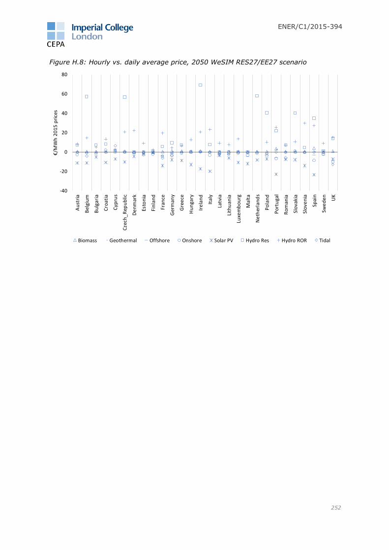
ENER/C1/2015-394

252

Figure H.8: Hourly vs. daily average price, 2050 WeSIM RES27/EE27 scenario

-40

-20

0

20

40

60

80A

ust

ria

Bel

giu

m

Bu

lgar

ia

Cro

atia

Cyp

rus

Cze

ch_

Rep

ub

lic

De

nm

ark

Esto

nia

Fin

lan

d

Fran

ce

Ger

man

y

Gre

ece

Hu

nga

ry

Ire

lan

d

Ital

y

Latv

ia

Lith

uan

ia

Luxe

mb

ou

rg

Mal

ta

Ne

ther

lan

ds

Po

lan

d

Po

rtu

gal

Ro

man

ia

Slo

vaki

a

Slo

ven

ia

Spai

n

Swe

de

n

UK

€/M

Wh

20

15

pri

ces


ENER/C1/2015-394

253

References ACER (2013), Capacity Remuneration Mechanisms and the Internal Market for Electricity,

Agency for the Cooperation of Energy Regulators, July 2013

http://www.acer.europa.eu/official_documents/acts_of_the_agency/publication/crms%2

0and%20the%20iem%20report%20130730.pdf

Borenstein (2008), The market value and cost of solar photovoltaic electricity

production, Borenstein, S., Center for the Study of Energy Markets Working Paper #176,

University of California Energy Institute, January 2008

Castro et al (2011), Reliability-driven transmission investment in systems with wind

generation, M. Castro, D. Pudjianto, P. Djapic, G. Strbac, IET Generation Transmission &

Distribution, Vol: 5, pp. 850-859, August 2011

CEER (2016), Key support elements of RES in Europe: moving towards market

integration, Council of European Energy Regulators, January 2016

http://www.ceer.eu/portal/page/portal/EER_HOME/EER_PUBLICATIONS/CEER_PAPERS/E

lectricity/2016/C15_SDE-49-

03%20CEER%20report%20on%20key%20support%20elements_26_January_2016.pdf

CEPA (2011), Note on impacts of the CfD FIT support package on costs and availability

of capital and on existing discounts in power purchase agreements, Cambridge Economic

Policy Associates, June 2011

https://www.gov.uk/government/uploads/system/uploads/attachment_data/file/48136/2

174-cepa-paper.pdf

CEPA (2015a), Costs of a best new entrant peaking plan for the calendar year 2016,

Cambridge Economic Policy Associates, May 2015

http://www.cepa.co.uk/corelibs/download.class.php?source=PB&fileName=sysimgdocs/d

ocs/CER-NIAUR-Fixed-Cost-of-a-Best-New-Entrant-Peaking-Plant-

2015_pb141_1.pdf&file=CER%20NIAUR%20Fixed%20Cost%20of%20a%20Best%20Ne

w%20Entrant%20Peaking%20Plant%202015.pdf

CEPA (2015b), The Cost of Capital for the 2016 BNE peaking plant, Cambridge Economic

Policy Associates, September 2015

http://www.cepa.co.uk/corelibs/download.class.php?source=PB&fileName=sysimgdocs/d

ocs/CER-NIAUR-Final-Report-WACC-

2015_pb141_2.pdf&file=CER%20NIAUR%20Final%20Report%20WACC%202015.pdf

DiaCore (2016), The impact of risks in renewable energy investments and the role of

smart policies, Paul Noothout, David de Jager, Lucie Tesnière, Sascha van Rooijen and

Nikolaos Karypidis (Ecofys) Robert Brückmann and Filip Jirouš (eclareon) Barbara

Breitschopf (Fraunhofer ISI) Dimitrios Angelopoulos and Haris Doukas (EPU-NTUA) Inga

Konstantinavičiūtė (LEI) Gustav Resch (TU Wien), February 2016

http://www.ecofys.com/files/files/diacore-2016-impact-of-risk-in-res-investments.pdf

DNV-GL (2014), Integration of Renewable Energy in Europe, Report No. 9011-700, June

2014

https://ec.europa.eu/energy/sites/ener/files/documents/201406_report_renewables_inte

gration_europe.pdf

Empower Demand (2011), The potential of smart meter enabled programs to increase

energy and systems efficiency: a mass pilot comparison, Stromback J., Dromacque C.,

Yassin M.H., VaasaETT, Global Energy Think Tank, 2011

http://esmig.eu/sites/default/files/2011.10.12_empower_demand_report_final.pdf

http://www.acer.europa.eu/official_documents/acts_of_the_agency/publication/crms%20and%20the%20iem%20report%20130730.pdf

http://www.acer.europa.eu/official_documents/acts_of_the_agency/publication/crms%20and%20the%20iem%20report%20130730.pdf

http://www.ceer.eu/portal/page/portal/EER_HOME/EER_PUBLICATIONS/CEER_PAPERS/Electricity/2016/C15_SDE-49-03%20CEER%20report%20on%20key%20support%20elements_26_January_2016.pdf



https://www.gov.uk/government/uploads/system/uploads/attachment_data/file/48136/2174-cepa-paper.pdf

https://www.gov.uk/government/uploads/system/uploads/attachment_data/file/48136/2174-cepa-paper.pdf

http://www.cepa.co.uk/corelibs/download.class.php?source=PB&fileName=sysimgdocs/docs/CER-NIAUR-Fixed-Cost-of-a-Best-New-Entrant-Peaking-Plant-2015_pb141_1.pdf&file=CER%20NIAUR%20Fixed%20Cost%20of%20a%20Best%20New%20Entrant%20Peaking%20Plant%202015.pdf




http://www.cepa.co.uk/corelibs/download.class.php?source=PB&fileName=sysimgdocs/docs/CER-NIAUR-Final-Report-WACC-2015_pb141_2.pdf&file=CER%20NIAUR%20Final%20Report%20WACC%202015.pdf



http://www.ecofys.com/files/files/diacore-2016-impact-of-risk-in-res-investments.pdf

https://ec.europa.eu/energy/sites/ener/files/documents/201406_report_renewables_integration_europe.pdf

https://ec.europa.eu/energy/sites/ener/files/documents/201406_report_renewables_integration_europe.pdf

http://esmig.eu/sites/default/files/2011.10.12_empower_demand_report_final.pdf

ENER/C1/2015-394

254

EC (2014), Communication from the Commission, Guidelines on State aid for

environmental protection and energy 2014-2020, 2014/C 200/01

EC (2014b) 356, Benchmarking smart metering deployment in the EU-27 with a focus on

electricity, COM/2014/0356

Ecofys (2016), European outlook - Trends in support systems for renewable electricity,

Dr. Klessmann D., Dansk Energi Workshop

http://www.danskenergi.dk/~/media/Uddannelse/1057/Corinna_Klessman.ashx

ENTSO-E (2015), 2015 Scenario Outlook & Adequacy Forecast, ENTSO-E, June 2015

https://www.entsoe.eu/Documents/SDC%20documents/SOAF/150630_SOAF_2015_publ

ication_wcover.pdf

ENTSO-E (2016), Project list TYNDP2016 for assessment,

https://www.entsoe.eu/Documents/TYNDP%20documents/TYNDP%202016/rgips/Project

%20list%20TYNDP2016%20assessments.xlsx?Web=1

EPRI (2009), Assessment of Achievable Potential from Energy Efficiency and Demand

Response Programs in the U.S. (2010-2030), Electric Power Research Institute, January

2009

http://www.edisonfoundation.net/iee/Documents/EPRI_SummaryAssessmentAchievable

EEPotential0109.pdf

EWEA (2014), EWEA Position paper on priority dispatch of wind power, EWEA Position

paper on priority dispatch of wind power, EWEA, 2014

EWEA (2015), Balancing responsibility and costs of wind power plants, European Wind

Energy Association, September 2015

EWI (2012), Flexibility options in European electricity markets in high RES-E scenarios,

Study on behalf of the International Energy Agency (IEA), October 2012

http://www.ewi.uni-

koeln.de/fileadmin/user_upload/Publikationen/Studien/Politik_und_Gesellschaft/2012/Fle

xibility_options_in_the_European_electricity_markets.pdf

Faruqui (2013), Dynamic Pricing – The bridge to a smart energy future, Faruqui A, The

Brattle Group, September 2013

Gils (2014), Assessment of the theoretical demand response potential in Europe, Gils H.,

Energy 67 (2014) 1-18.

Green and Vasilakos (2012), Storing Wind for a Rainy Day: What kind of electricity does

Denmark export? Green, R., Vasilakos, N.V., Energy Journal, Volume 33, Issue 3,

January 2012

Hirth (2013), The market value of variable renewables: The effect of solar wind power

variability on their relative price, Hirth, L., Energy Economics, 38, pp. 218-236, July

2013

IESO (Sep 2015), Part 12.0: Demand Response Auction, September 2015

http://www.ieso.ca/Documents/imowebpub/201509%20DRA/MAN-44_v0.2.pdf

IRENA (2015), Battery storage for renewables: market status and technology outlook,

http://www.danskenergi.dk/~/media/Uddannelse/1057/Corinna_Klessman.ashx

https://www.entsoe.eu/Documents/SDC%20documents/SOAF/150630_SOAF_2015_publication_wcover.pdf

https://www.entsoe.eu/Documents/SDC%20documents/SOAF/150630_SOAF_2015_publication_wcover.pdf

https://www.entsoe.eu/Documents/TYNDP%20documents/TYNDP%202016/rgips/Project%20list%20TYNDP2016%20assessments.xlsx?Web=1

https://www.entsoe.eu/Documents/TYNDP%20documents/TYNDP%202016/rgips/Project%20list%20TYNDP2016%20assessments.xlsx?Web=1

http://www.edisonfoundation.net/iee/Documents/EPRI_SummaryAssessmentAchievableEEPotential0109.pdf

http://www.edisonfoundation.net/iee/Documents/EPRI_SummaryAssessmentAchievableEEPotential0109.pdf

http://www.ewi.uni-koeln.de/fileadmin/user_upload/Publikationen/Studien/Politik_und_Gesellschaft/2012/Flexibility_options_in_the_European_electricity_markets.pdf



http://www.ieso.ca/Documents/imowebpub/201509%20DRA/MAN-44_v0.2.pdf

ENER/C1/2015-394

255

Technical Report January, International Renewable Energy Agency (IRENA), January

2015,

http://www.irena.org/documentdownloads/publications/irena_battery_storage_report_2

015.pdf

JRC (2013a), Assessment of the European potential for pumped hydropower energy

storage, A GIS-based assessment of pumped hydropower storage potential, Gimeno-

Gutiérrez M, Lacal-Arántegui R., 2013

https://ec.europa.eu/jrc/sites/jrcsh/files/jrc_20130503_assessment_european_phs_pote

ntial.pdf

JRC (2013b), Report on Innovative Financial Instruments for the Implementation of the

SET Plan, First-Of-A-Kind Projects”, J. Burnham, O. Debande, O. Jones, C. Mihai, J.

Moore, I. Temperton, 2013

https://setis.ec.europa.eu/sites/default/files/reports/Set-Plan-Financial-Instruments.pdf

Katipamula and Lu (2006), Evaluation of Residential HVAC Control Strategies for

Demand Response Programs (SYMPOSIUM PAPERS - CH06-7 Demand Response

Strategies for Building Systems), Katipamula L, Lu N., ASHRAE Transactions 112:535-

546, February 2006

KPMG (2015), Cost of Capital Study 2015 Value enhancement in the interplay of risks

and returns, https://assets.kpmg.com/content/dam/kpmg/pdf/2016/01/kpmg-cost-of-

capital-study-2015.pdf

Kremer and Nyborg (2004), Underpricing and Market Power in Uniform Price Auctions,

Kremer, I., & Nyborg, K.G., The Review of Financial Studies 17(3): pp.849-877, 2004.

Moreno (2008), Cost of capital indicator for EU member states – methodology, Moreno

G. D., Joint Research Centre, 2008

http://publications.jrc.ec.europa.eu/repository/bitstream/JRC49398/reqno_jrc49398_cos

t_of_capital_-_methodology_final.doc_1_%5B1%5D.pdf

Moreno and Loschky (2010), Cost of Capital Indicator for EU Member States, Moreno G.,

Loschky A., 2010

http://bookshop.europa.eu/en/cost-of-capital-indicator-for-eu-member-states-

pbLBNA24322/

NERA (2013), Changes in Hurdle Rates for Low Carbon

Generation Technologies due to the Shift from the UK Renewables Obligation to a

Contracts for Difference Regime, December 2013

https://www.gov.uk/government/uploads/system/uploads/attachment_data/file/267606/

NERA_Report_Assessment_of_Change_in_Hurdle_Rates_-_FINAL.pdf

Newbery (2015), Security of Supply, Capacity Auctions and Interconnectors, Newbery

N., EPRG Working Paper, Cambridge Working Paper 1508, University of Cambridge,

February 2015

http://www.eprg.group.cam.ac.uk/wp-content/uploads/2015/03/EPRG-WP-1508.pdf

Newbery (2010), The role of carbon markets in preventing dangerous climate change,

Environmental Audit Committee, Memorandum submitted by David Newbery.

http://www.publications.parliament.uk/pa/cm200910/cmselect/cmenvaud/290/290we33

.htm

http://www.irena.org/documentdownloads/publications/irena_battery_storage_report_2015.pdf

http://www.irena.org/documentdownloads/publications/irena_battery_storage_report_2015.pdf

https://ec.europa.eu/jrc/sites/jrcsh/files/jrc_20130503_assessment_european_phs_potential.pdf

https://ec.europa.eu/jrc/sites/jrcsh/files/jrc_20130503_assessment_european_phs_potential.pdf

https://setis.ec.europa.eu/sites/default/files/reports/Set-Plan-Financial-Instruments.pdf



http://publications.jrc.ec.europa.eu/repository/bitstream/JRC49398/reqno_jrc49398_cost_of_capital_-_methodology_final.doc_1_%5B1%5D.pdf

http://publications.jrc.ec.europa.eu/repository/bitstream/JRC49398/reqno_jrc49398_cost_of_capital_-_methodology_final.doc_1_%5B1%5D.pdf

http://bookshop.europa.eu/en/cost-of-capital-indicator-for-eu-member-states-pbLBNA24322/

http://bookshop.europa.eu/en/cost-of-capital-indicator-for-eu-member-states-pbLBNA24322/



http://www.eprg.group.cam.ac.uk/wp-content/uploads/2015/03/EPRG-WP-1508.pdf

http://www.publications.parliament.uk/pa/cm200910/cmselect/cmenvaud/290/290we33.htm

http://www.publications.parliament.uk/pa/cm200910/cmselect/cmenvaud/290/290we33.htm

ENER/C1/2015-394

256

Schmalensee (2014), The Performance of US Wind and Solar Generating Plants,

Schmalensee, R., Sloan School of Management, Massachusetts Institute of Technology,

August 2014

https://www.hks.harvard.edu/hepg/Papers/2014/Schmalensee%20%20--

%20%20Wind%20%20Solar%20--%20final.pdf

SEDC (2015), Mapping Demand Response in Europe Today 2015, Smart Energy Demand

Coalition, 2015

http://www.smartenergydemand.eu/wp-content/uploads/2015/09/Mapping-Demand-

Response-in-Europe-Today-2015.pdf

Strbac et al (2012), Strategic assessment of the role and value of energy storage

systems in the UK low carbon energy future, Strbac, G., Aunedi, M., Pudjianto, D.,

Djapic, P., Teng, F., Sturt, A., Jackravut, D., Sansom, R., Yufit, V. and Brandon, N.,

Report for Carbon Trust, June 2012

https://www.carbontrust.com/media/129310/energy-storage-systems-role-value-

strategic-assessment.pdf

Sturt and Srbac (2012a), Efficient Stochastic Scheduling for Simulation of Wind-

Integrated Power Systems, A. Sturt, G. Strbac , IEEE Transactions on Power Systems,

Vol: 27, pp. 323-334, February 2012.

Sturt and Srbac (2012b), Value of stochastic reserve policies in low-carbon power

systems”, A. Sturt, G. Strbac, Proceedings of the Institution of Mechanical Engineers:

Part O-Journal of Risk and Reliability, Vol: 226, pp. 51-64, February 2012.

Rastler (2010), Electricity energy storage technology options: a white paper primer on

applications, costs and benefits, Rastler, D.M., Electric Power Research Institute,

December 2010

http://large.stanford.edu/courses/2012/ph240/doshay1/docs/EPRI.pdf

Tierny et al. (2008), Uniform-Pricing versus Pay-as-Bid in Wholesale Electricity Markets:

Does it Make a Difference? Tierney, S.F., Schatski, T., Mukerji, R, March 2008

http://www.nyiso.com/public/webdocs/media_room/current_issues/uniformpricing_v_pa

yasbid_tierneyschatzkimukerji_2008.pdf

US DOE (2012), Demand Response Assessment for Eastern Interconnection, Oak Ridge

National Laboratory, US Department of Energy, September 2012

http://energy.gov/sites/prod/files/2013/05/f1/2012LAAR-Baek.pdf

Wind Europe (2016), Offshore wind post-2020 cost reductions, presentation provided by

the Commission, Wind Europe, 2016

Wirth (2016), Recent Facts about Photovoltaics in Germany, Fraunhofer Institute for

Solar Energy Systems ISE (in German), Wirth, H., May 2016

http://www.pv-magazine.com/news/details/beitrag/-renewables-peak-at-95-of-german-

electricity-demand-_100024484/#axzz4DlRNH973

https://www.hks.harvard.edu/hepg/Papers/2014/Schmalensee%20%20--%20%20Wind%20%20Solar%20--%20final.pdf

https://www.hks.harvard.edu/hepg/Papers/2014/Schmalensee%20%20--%20%20Wind%20%20Solar%20--%20final.pdf

http://www.smartenergydemand.eu/wp-content/uploads/2015/09/Mapping-Demand-Response-in-Europe-Today-2015.pdf

http://www.smartenergydemand.eu/wp-content/uploads/2015/09/Mapping-Demand-Response-in-Europe-Today-2015.pdf

https://www.carbontrust.com/media/129310/energy-storage-systems-role-value-strategic-assessment.pdf

https://www.carbontrust.com/media/129310/energy-storage-systems-role-value-strategic-assessment.pdf

http://large.stanford.edu/courses/2012/ph240/doshay1/docs/EPRI.pdf

http://www.nyiso.com/public/webdocs/media_room/current_issues/uniformpricing_v_payasbid_tierneyschatzkimukerji_2008.pdf

http://www.nyiso.com/public/webdocs/media_room/current_issues/uniformpricing_v_payasbid_tierneyschatzkimukerji_2008.pdf

http://energy.gov/sites/prod/files/2013/05/f1/2012LAAR-Baek.pdf

