1

Supporting Information:

A Highly Sensitive Graphene Woven Fabric Strain Sensor for Wearable Wireless

Musical Instrument

Xu Liu1, Chen Tang1, Xiaohan Du1, Shuai Xiong1, Siyuan Xi1, Yuefeng Liu1, Xi Shen1, Qingbin Zheng1,2,*, Zhenyu Wang1, Ying Wu1, Andrew Horner3, and Jang-Kyo Kim1,*

1 Department of Mechanical and Aerospace Engineering, The Hong Kong University of Science and Technology, Clear Water Bay, Kowloon, Hong Kong

2 Institute for Advanced Study, The Hong Kong University of Science and Technology, Clear Water Bay, Hong Kong

3 Department of Computer Science and Engineering, The Hong Kong University of Science and Technology, Clear Water Bay, Hong Kong

*Corresponding author: Fax: +852 2358 1543; email: mezheng@ust.hk (QB Zheng)

mejkkim@ust.hk (J-K Kim)

Electronic Supplementary Material (ESI) for Materials Horizons.This journal is © The Royal Society of Chemistry 2017

2

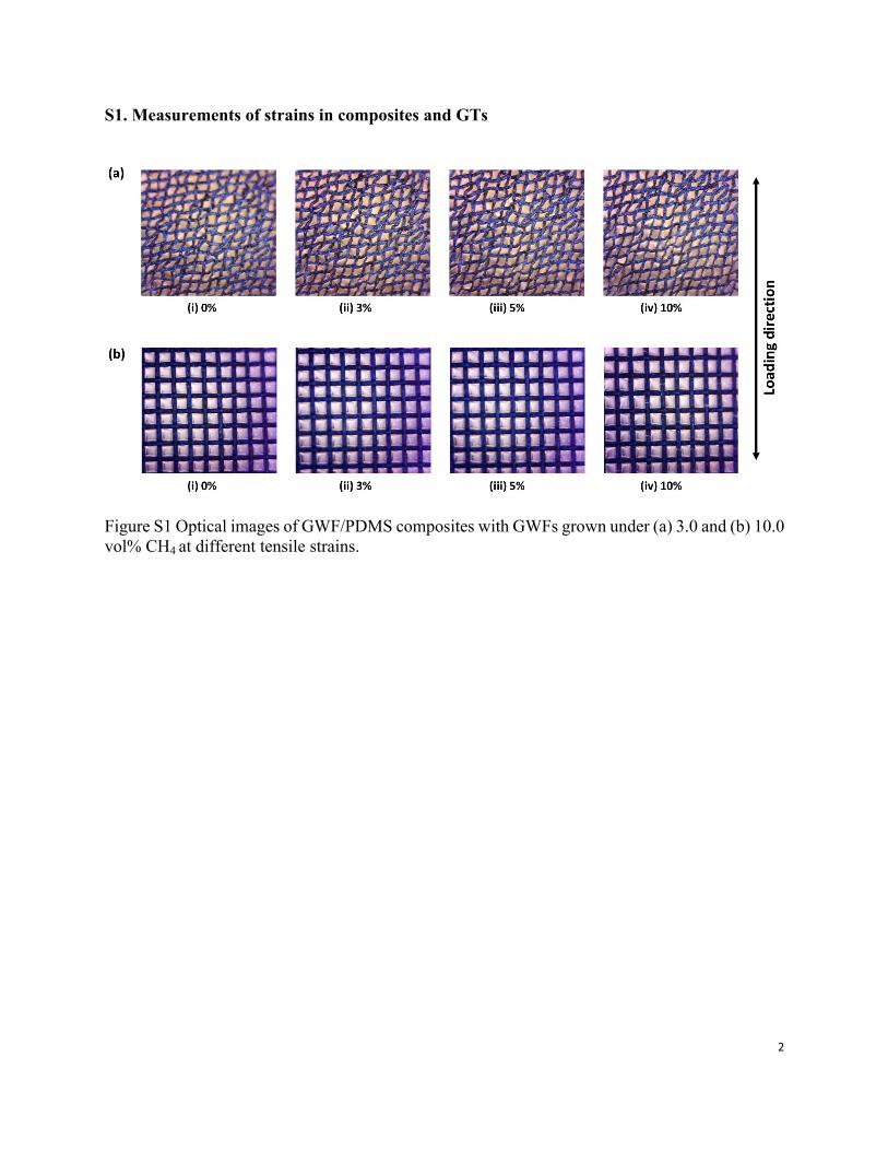
S1. Measurements of strains in composites and GTs

Figure S1 Optical images of GWF/PDMS composites with GWFs grown under (a) 3.0 and (b) 10.0 vol% CH4 at different tensile strains.

3

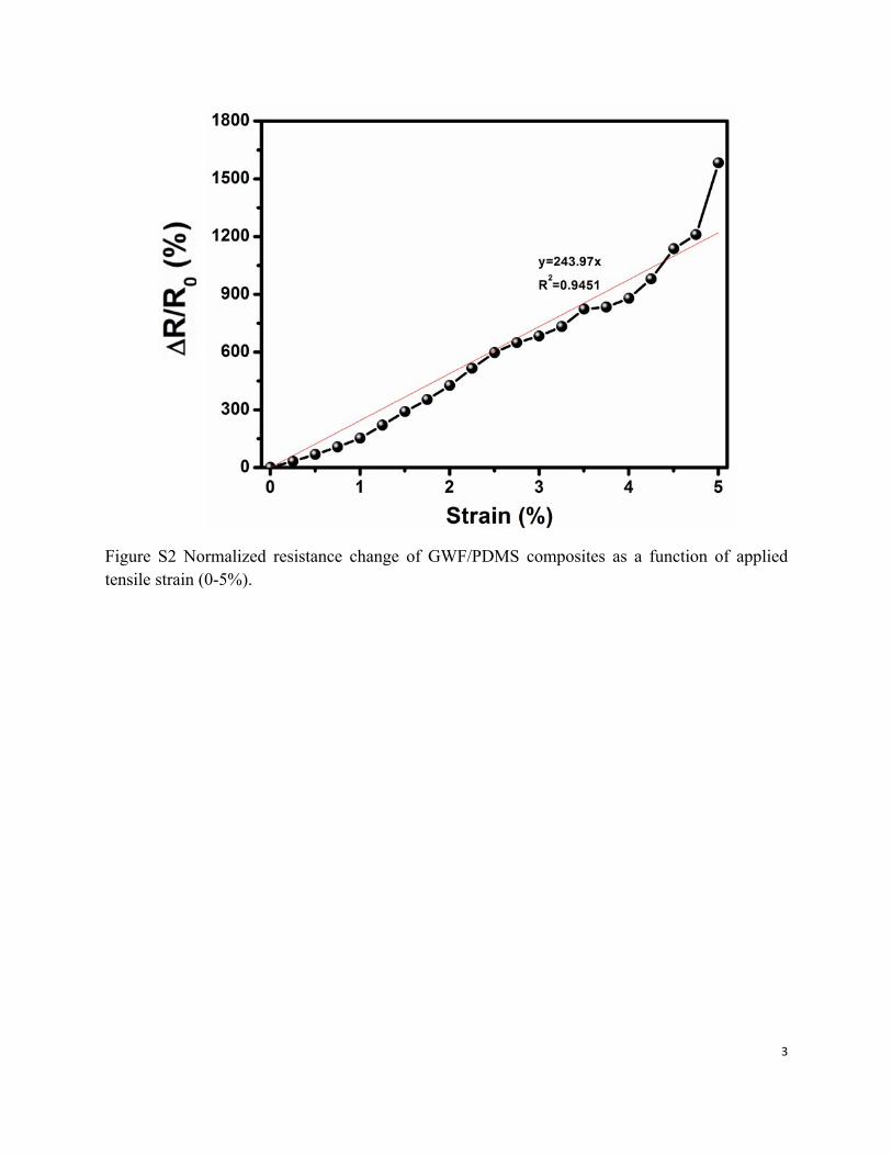
Figure S2 Normalized resistance change of GWF/PDMS composites as a function of applied tensile strain (0-5%).

4

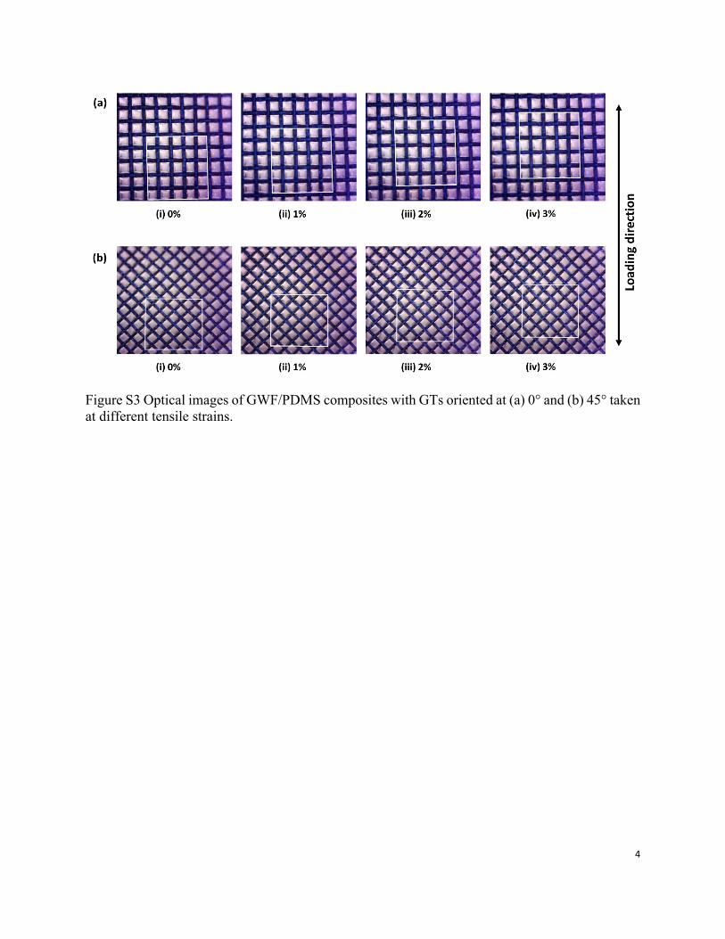
Figure S3 Optical images of GWF/PDMS composites with GTs oriented at (a) 0° and (b) 45° taken at different tensile strains.

5

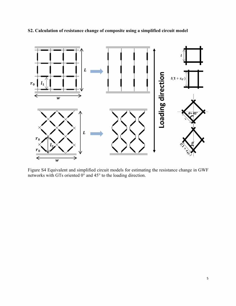
S2. Calculation of resistance change of composite using a simplified circuit model

Figure S4 Equivalent and simplified circuit models for estimating the resistance change in GWF networks with GTs oriented 0° and 45° to the loading direction.

6

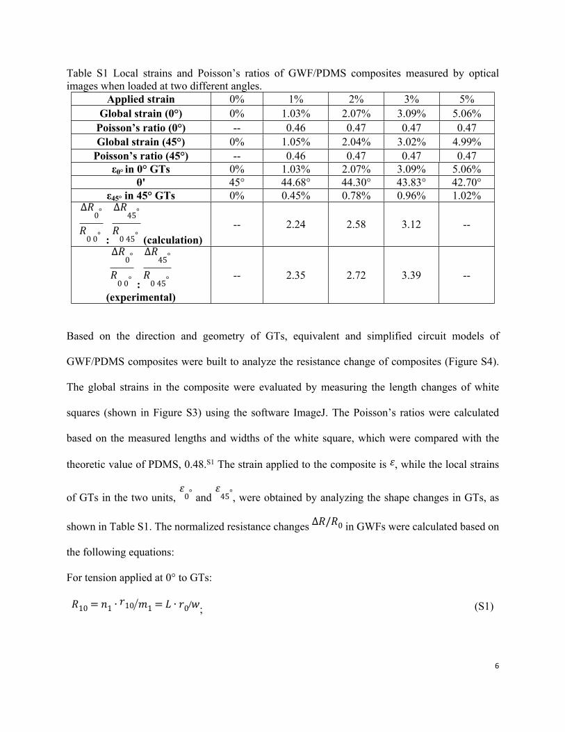
Table S1 Local strains and Poisson’s ratios of GWF/PDMS composites measured by optical images when loaded at two different angles.

Applied strain 0% 1% 2% 3% 5%Global strain (0°) 0% 1.03% 2.07% 3.09% 5.06%

Poisson’s ratio (0°) -- 0.46 0.47 0.47 0.47Global strain (45°) 0% 1.05% 2.04% 3.02% 4.99%

Poisson’s ratio (45°) -- 0.46 0.47 0.47 0.47ε0° in 0° GTs 0% 1.03% 2.07% 3.09% 5.06%

θ' 45° 44.68° 44.30° 43.83° 42.70°ε45° in 45° GTs 0% 0.45% 0.78% 0.96% 1.02%

: (calculation)

∆𝑅0°

𝑅0 0°

∆𝑅45°

𝑅0 45°

-- 2.24 2.58 3.12 --

:

∆𝑅0°

𝑅0 0°

∆𝑅45°

𝑅0 45°

(experimental)

-- 2.35 2.72 3.39 --

Based on the direction and geometry of GTs, equivalent and simplified circuit models of

GWF/PDMS composites were built to analyze the resistance change of composites (Figure S4).

The global strains in the composite were evaluated by measuring the length changes of white

squares (shown in Figure S3) using the software ImageJ. The Poisson’s ratios were calculated

based on the measured lengths and widths of the white square, which were compared with the

theoretic value of PDMS, 0.48.S1 The strain applied to the composite is , while the local strains 𝜀

of GTs in the two units, and , were obtained by analyzing the shape changes in GTs, as 𝜀

0° 𝜀45°

shown in Table S1. The normalized resistance changes in GWFs were calculated based on ∆𝑅/𝑅0

the following equations:

For tension applied at 0° to GTs:

;𝑅10 = 𝑛1 ∙ 𝑟10 𝑚1 = 𝐿 ∙ 𝑟0 𝑤 (S1)

7

;𝑟1𝑠 = 𝑟0 + 𝑘 ∙ 𝜀

0° (S2)

;𝑅1𝑠 = 𝑛1 ∙ 𝑟1𝑠 𝑚1 = 𝐿 ∙ 𝑟1𝑠 𝑤 (S3)

.

∆𝑅0°

𝑅0 0°

= ∆𝑅1 𝑅10 = (𝑅1𝑠 ‒ 𝑅10) 𝑅10 = (𝑟1𝑠 ‒ 𝑟0) 𝑟0 = ∆𝑟1 𝑟0 = 𝑘 ∙ 𝜀0° (S4)

For tension applied at 45° to GTs:

;𝑅20 = 𝑛2 ∙ 𝑟0 𝑚2 = 𝐿 ∙ 𝑟0 𝑤 (S5)

;𝑟2𝑠 = 𝑟0 + 𝑘 ∙ 𝜀

45° (S6)

;𝑅2𝑠 = 𝑛2 ∙ 𝑟2𝑠 𝑚2 = 𝐿 ∙ 𝑟2𝑠 𝑤 (S7)

.

∆𝑅45°

𝑅0 45°

= ∆𝑅2 𝑅20 = (𝑅2𝑠 ‒ 𝑅20) 𝑅20 = (𝑟2𝑠 ‒ 𝑟0) 𝑟0 = ∆𝑟2 𝑟0 = 𝑘 ∙ 𝜀45° (S8)

where are the resistances before and after tension, and resistance change of 𝑅0, 𝑅𝑠, ∆𝑅

GWF/PDMS composites; are the resistances before and after tension, and resistance 𝑟0, 𝑟𝑠, ∆𝑟

change of GTs, respectively; and are the length and width of GWFs; and are the numbers 𝐿 𝑤 𝑛 𝑚

of the units in the length and width directions, respectively. According to the calculation, the

normalized resistance changes of GWF/PDMS composites with different GT orientations depend

on local strains of GTs arising from the deformation in the composite.

S3. Calculation of the local strain in GTs with different orientations

The relationship between the strain applied to the composite, , and the local strains in GTs were 𝜀

established using the strain transformation equation:

8

,𝜀𝜃 =

𝜀𝑥 + 𝜀𝑦

2+ (𝜀𝑥 ‒ 𝜀𝑦

2 )cos 2𝜃 +𝜀𝑥𝑦

2sin 2𝜃 (S9)

where and are strains along the x- and y-directions, respectively, and is the shear strain. 𝜀𝑥 𝜀𝑦 𝜀𝑥𝑦

Under uniaxial tension,

,𝜀𝑥 = 𝜀 (S10)

,𝜀𝑦 =‒ 𝑣𝜀 (S11)

, 𝜀𝑥𝑦 = 0 (S12)

When the loading direction is the same as the GT direction, the local strain in GTs is given by:

.𝜀

0° = 𝜀𝑥 = 𝜀 (S13)

When the loading direction is 45 to the GTs, the local strain in GTs is given by:

= , 𝜀

45° =𝜀 ‒ 𝑣𝜀

2+ (𝜀 + 𝑣𝜀

2 )cos 2𝜃' (1 ‒ 𝑣

2+

1 + 𝑣2

cos 2𝜃')𝜀 (S14)

where is the angle between the GTs and the loading direction after loading. The external load 𝜃'

induced the shape change of the orthogonal structure of GTs, leading to the change of angle

between GTs, as shown in Figure S3. The angle between the GT and the loading direction after

loading is obtained by the geometric relationship:

. tan 𝜃' =

1 ‒ 𝑣𝜀1 + 𝜀 (S15)

S4. Cyclic performance of GWF/PDMS composites

9

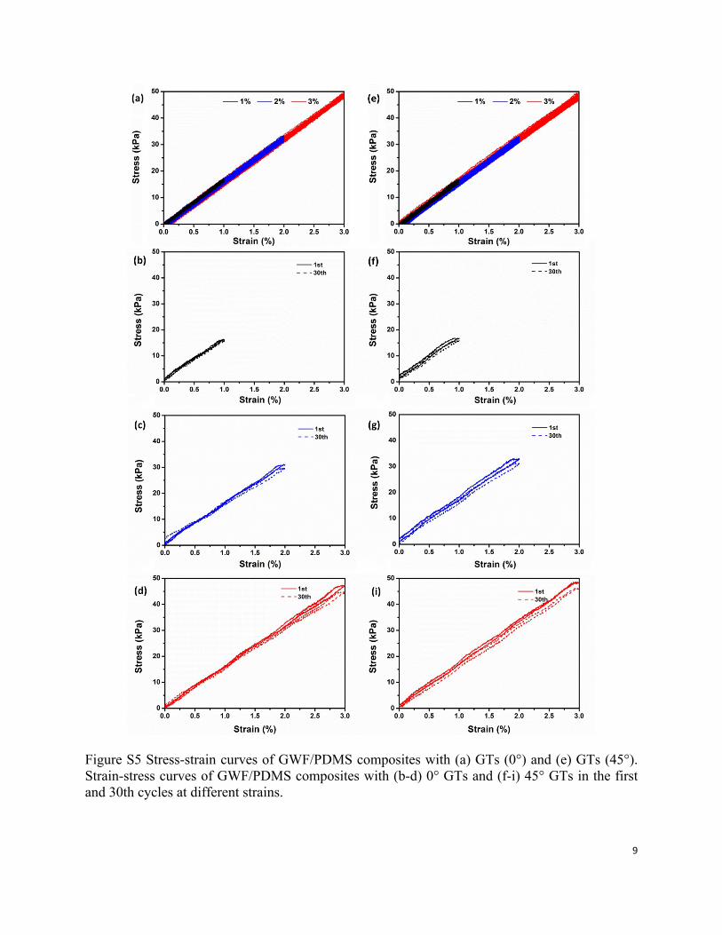
Figure S5 Stress-strain curves of GWF/PDMS composites with (a) GTs (0°) and (e) GTs (45°). Strain-stress curves of GWF/PDMS composites with (b-d) 0° GTs and (f-i) 45° GTs in the first and 30th cycles at different strains.

10

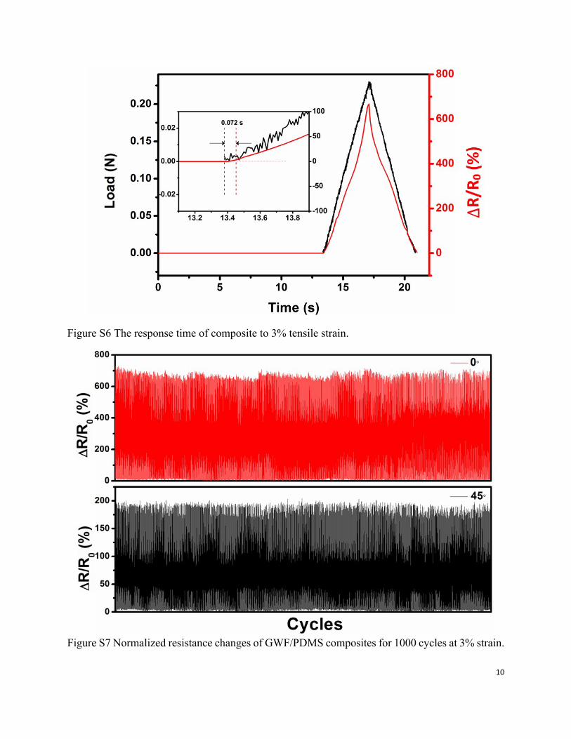
Figure S6 The response time of composite to 3% tensile strain.

Figure S7 Normalized resistance changes of GWF/PDMS composites for 1000 cycles at 3% strain.

11

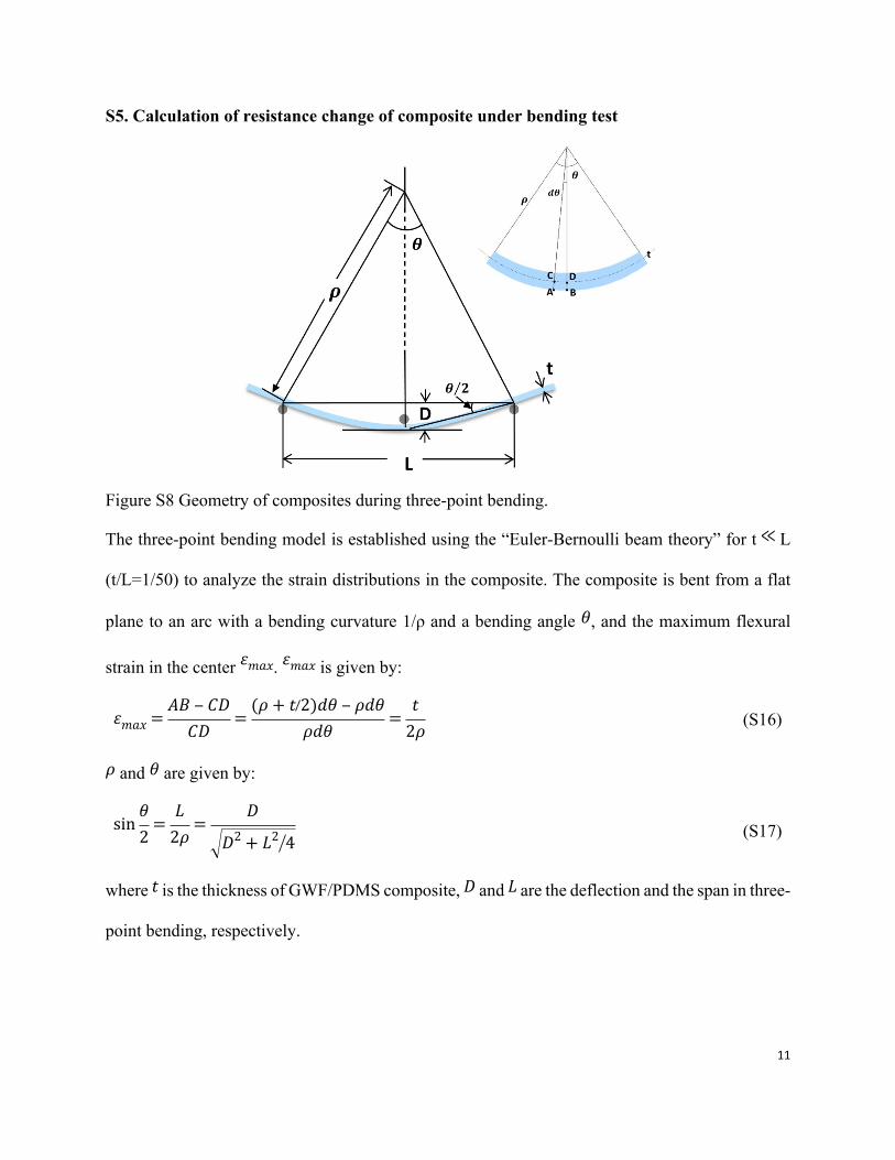
S5. Calculation of resistance change of composite under bending test

Figure S8 Geometry of composites during three-point bending.

The three-point bending model is established using the “Euler-Bernoulli beam theory” for t L ≪

(t/L=1/50) to analyze the strain distributions in the composite. The composite is bent from a flat

plane to an arc with a bending curvature 1/ρ and a bending angle , and the maximum flexural 𝜃

strain in the center . is given by:𝜀𝑚𝑎𝑥 𝜀𝑚𝑎𝑥

𝜀𝑚𝑎𝑥 =

𝐴𝐵 ‒ 𝐶𝐷𝐶𝐷

=(𝜌 + 𝑡 2)𝑑𝜃 ‒ 𝜌𝑑𝜃

𝜌𝑑𝜃=

𝑡2𝜌

(S16)

and are given by: 𝜌 𝜃

sin

𝜃2

=𝐿

2𝜌=

𝐷

𝐷2 + 𝐿2 4(S17)

where is the thickness of GWF/PDMS composite, and are the deflection and the span in three-𝑡 𝐷 𝐿

point bending, respectively.

12

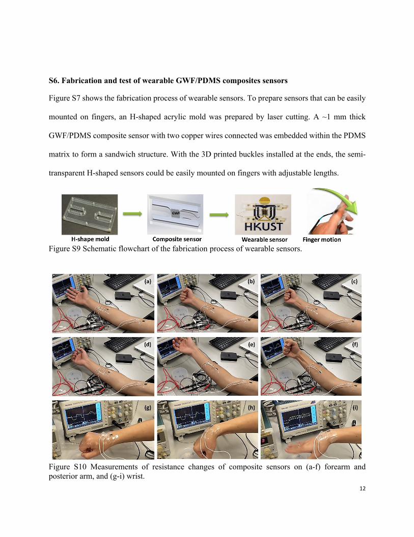
S6. Fabrication and test of wearable GWF/PDMS composites sensors

Figure S7 shows the fabrication process of wearable sensors. To prepare sensors that can be easily

mounted on fingers, an H-shaped acrylic mold was prepared by laser cutting. A ~1 mm thick

GWF/PDMS composite sensor with two copper wires connected was embedded within the PDMS

matrix to form a sandwich structure. With the 3D printed buckles installed at the ends, the semi-

transparent H-shaped sensors could be easily mounted on fingers with adjustable lengths.

Figure S9 Schematic flowchart of the fabrication process of wearable sensors.

Figure S10 Measurements of resistance changes of composite sensors on (a-f) forearm and posterior arm, and (g-i) wrist.

13

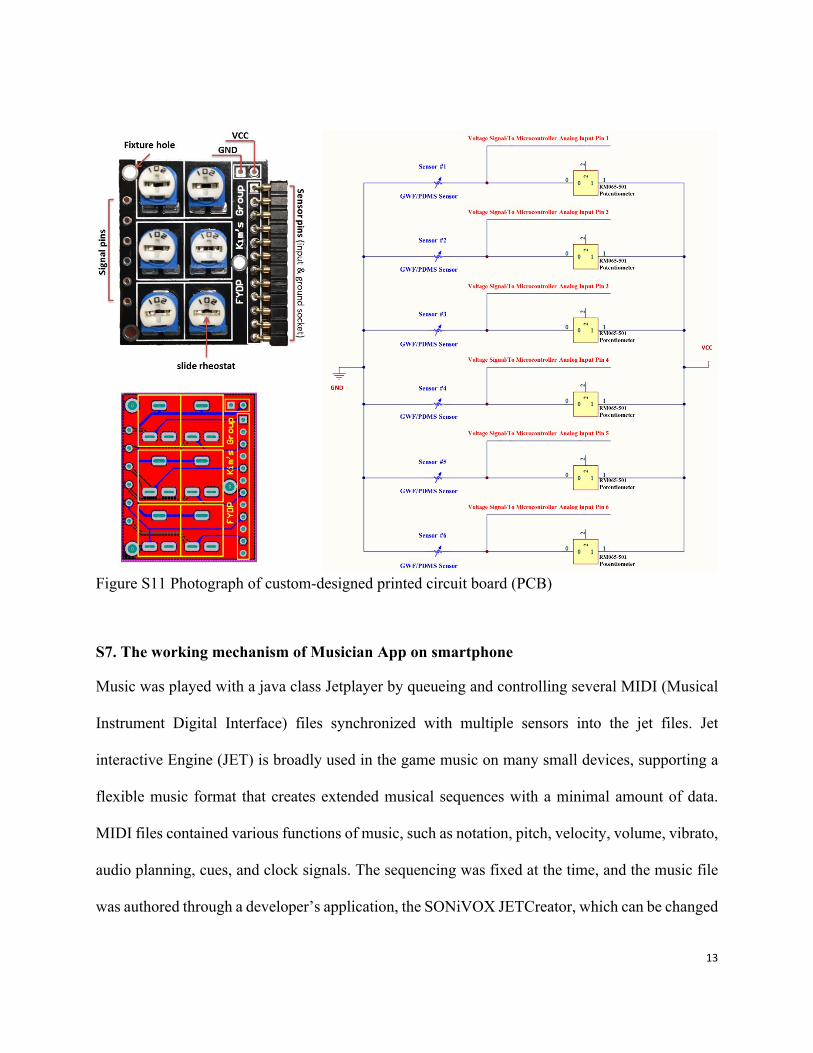
Figure S11 Photograph of custom-designed printed circuit board (PCB)

S7. The working mechanism of Musician App on smartphone

Music was played with a java class Jetplayer by queueing and controlling several MIDI (Musical

Instrument Digital Interface) files synchronized with multiple sensors into the jet files. Jet

interactive Engine (JET) is broadly used in the game music on many small devices, supporting a

flexible music format that creates extended musical sequences with a minimal amount of data.

MIDI files contained various functions of music, such as notation, pitch, velocity, volume, vibrato,

audio planning, cues, and clock signals. The sequencing was fixed at the time, and the music file

was authored through a developer’s application, the SONiVOX JETCreator, which can be changed

14

dynamically under the program controlled by the output signals arising from the body motion

sensors.

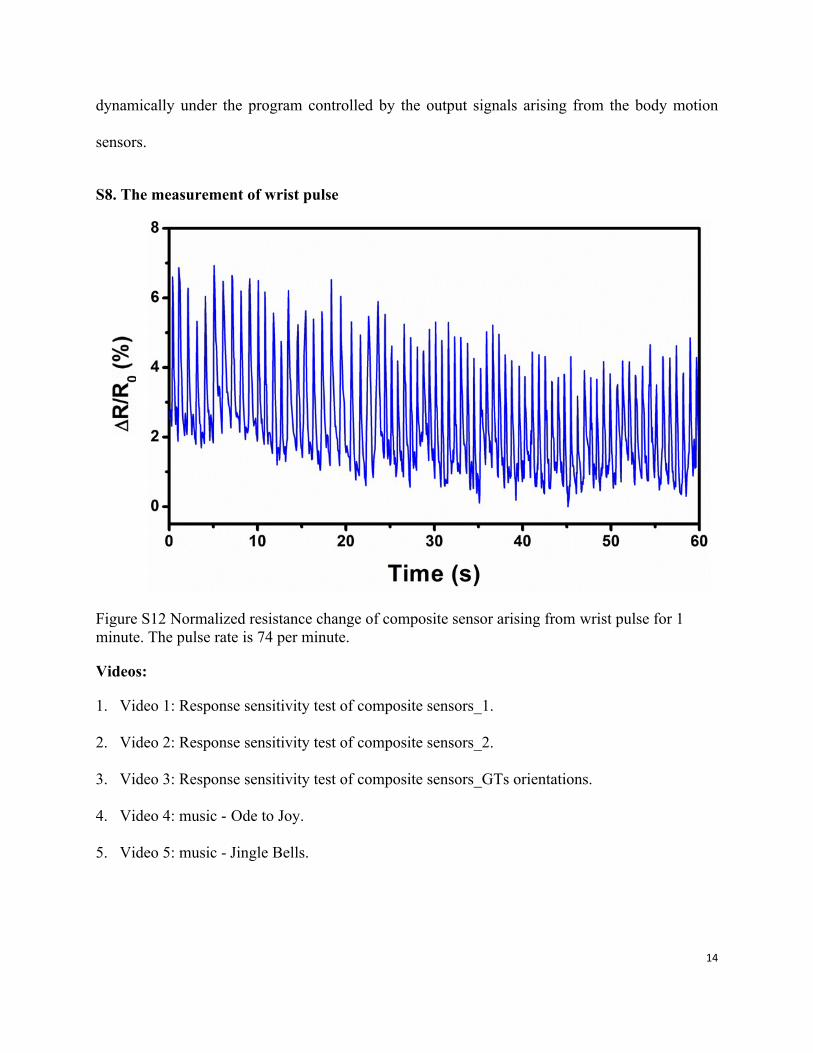
S8. The measurement of wrist pulse

Figure S12 Normalized resistance change of composite sensor arising from wrist pulse for 1 minute. The pulse rate is 74 per minute.

Videos:

1. Video 1: Response sensitivity test of composite sensors_1.

2. Video 2: Response sensitivity test of composite sensors_2.

3. Video 3: Response sensitivity test of composite sensors_GTs orientations.

4. Video 4: music - Ode to Joy.

5. Video 5: music - Jingle Bells.

15

[S1] N. Bowden, S. Brittain, A. G. Evans, J. Hutchinson and G. M. Whitesides, Nature, 1998,

393, 146-149.