Supporting Information

Examining the impacts of ethanol (E85) versus gasoline photochemical production of

smog in a fog using near-explicit gas- and aqueous-chemistry mechanisms

Diana L. Ginnebaugh, Mark Z. Jacobson

Atmosphere/Energy Program, Department of Civil and Environmental Engineering, Jerry Yang & Akiko Yamazaki Environment & Energy Building, 473 Via Ortega, MC 4020, Stanford University, Stanford, CA 94305, USA moongdes@stanford.edu, Jacobson@stanford.edu

Corresponding Author: Diana L Ginnebaugh, 473 Via Ortega, MC 4020, Stanford University, Stanford, CA 94305, moongdes@stanford.edu, Phone: (650) 721-2730, Fax: (650) 721-2730

Summary The supporting information document includes 1) a detailed description of the model used for this study, 2) additional model setup information including the tables of emissions, 3) discussion of the time-series results not included in the main paper, and 4) more sensitivity results.

1

1. Model Description This air pollution box model combines a near-explicit chemical mechanism with a sparse-matrix ordinary differential equation solver. 1A. Gas-Phase Chemical Mechanism Master Chemical Mechanism version 3.1 (MCM) The Master Chemical Mechanism (MCM) version 3.1 was chosen for this study because it is a near-explicit chemical mechanism that has been evaluated previously. MCM v. 3.1 (updated 2005) describes the tropospheric degradation of 135 commonly-emitted volatile organic compounds (VOCs) (Jenkin et al. 1997; MCM 2002; Jenkin et al. 2003; Saunders et al. 2003; Bloss et al. 2005b). It currently incorporates over 13,500 chemical reactions and over 4,600 species.

A number of studies have looked at the accuracy of the MCM v. 3 and v. 3.1 by comparing the model results with smog chamber data, including for the species examined here (Wagner et al. 2002; Bloss et al. 2005a; Bloss et al. 2005b; Hynes et al. 2005; Pinho et al. 2005; Pinho et al. 2006a; Pinho et al. 2006b; Pinho et al. 2007). The mechanism has also been used in a number of field studies, often in conjunction with a photochemical trajectory model (PTM), to assess ozone formation in the atmosphere (Derwent et al. 2003; Derwent et al. 2005; Derwent et al. 2007; Evtyugina et al. 2007) and to look at secondary organic aerosol formation (Jenkin 2004; Johnson et al. 2004; 2005; Johnson et al. 2006a; Johnson et al. 2006b). The uncertainties associated with the MCM have also been investigated (Zador et al. 2005). 1B. Aqueous-Phase Chemical Mechanism Chemical Aqueous Phase Radical Mechanism version 3.0i (CAPRAM) Chemical Aqueous Phase Radical Mechanism (CAPRAM) is a chemical mechanism that includes the aqueous reactions of inorganic and organic species that are present in the atmosphere. It is available on the internet: http://projects.tropos.de/capram/. CAPRAM 3.0i has been expanded from version 2.4 (Ervens et al. 2003) to include organic species with two to six carbon atoms (Herrmann et al. 2005). The original CAPRAM was developed in 1999 to work in conjunction with RADM2 to provide a more detailed mechanism that included aqueous reactions (Herrmann et al. 1999). Today’s CAPRAM 3.0i is coupled with RACM by the authors for a mechanism that deals with gas-phase and aqueous-phase reactions (Herrmann et al. 2005). We coupled CAPRAM 3.0i with MCM v. 3.1 instead of RACM because MCM is a more complete gas-phase chemistry mechanism and our ODE solver, SMVGEAR, is efficient enough to make it practical to use two large mechanisms.

CAPRAM 3.0i has the aqueous phase chemical reactions for 34 species – 13 monocarboxylic and dicarboxylic acids, 10 carbonyl compounds, 5 alcohols, 4 polyfunctional compounds, 1 ester and 1 heterocyclic compound (Tilgner and Herrmann 2007). It treats the aqueous chemistry among 390 species and 829 reactions, including 51 gas-to-aqueous phase reactions. One of the interesting results found by Hermann et al. (2005) was that the degradation of aldehydes and ketone in both the gas-phase and the aqueous-phase forms monocarboxylic and dicarboxylic compounds which build up in the aqueous phase. These results, and others, were not apparent with the previous version of CAPRAM because the chemicals dealt with in the aqueous phase were not extensive enough (Herrmann et al. 2005). CAPRAM is the most extensive aqueous phase mechanism available (Pilling 2007) and is therefore ideal for our study.

2

1C. Ordinary Differential Equation Solver Sparse-Matrix Vectorized Gear Solver (SMVGEAR II) To solve the large set of chemical equations in the MCM, we use SMVGEAR II, a sparse-matrix ordinary differential equation (ODE) solver (Jacobson and Turco 1994; Jacobson 1995; 1998). It was chosen for several reasons. First, it uses the Gear solution mechanism, which is considered a benchmark for accuracy. Second, it uses a sparse-matrix technique during matrix decomposition and backsubstitution that dramatically decreases the run times. Jacobson (1995; 1998) also describes other measures that SMVGEAR employs to decrease run time for 3D modeling, including grouping and reordering of cells. The speed of the ODE solver is very important for allowing a large mechanism such as MCM and CAPRAM to be used in urban, regional, and global 3-D models. 2. Model Setup for E85 versus Gasoline Comparisons In this section, the setup of the box model for comparing the effect of E85 versus gasoline is described. Since the emissions data were based on data from Jacobson’s study (2007), summarized in Table S1, the first step was to determine the emissions from gasoline and E85 with more explicit treatment than has been used previously. To do this, we used data from Black (1995-1997), which gives the speciated exhaust emissions for reformulated gasoline (RFG) in a Ford Taurus and for ethanol (E85) in a Ford Lumina Flex Fuel Vehicle (FFV) during the first 124 seconds of cold start. The data are summarized in Table S2.

We assumed that the speciation during a cold start is similar to that during the whole vehicle cycle, but the emission amounts differ because larger amounts of unburned emissions occur during cold start than during the whole driving cycle. The actual emissions are based on emissions data for current gasoline vehicles for the South Coast Air Basin (SCAB), moved forward to the year 2020, shown in Table S1. We assume that all of the vehicles change from gasoline to E85. The results can then be applied proportionally to any situation where a change is being made from gasoline to E85. To start separating the emissions data from Table S1 into more explicit species, we first used the Black emissions data for RFG and E85 to determine the percent of total organic gases (TOG) for each emitted species in the Black data, shown in Table S2. Unfortunately, there were many species measured whose chemical nature was not discernable. These species were lumped together and assumed to be unreactive. There were also some species in the Black data not included in the MCM, but this was a small fraction of the total amount of species in the emissions. Even though the MCM is a near-explicit chemical mechanism, it does not describe the degradation of all organic species (that would be impractical) – it concentrates on commonly-emitted species. For the ethanol (E85) emissions, the known species from Black’s data that also existed in the MCM made up a large portion (over 95%) of the TOG measured. For RFG, the known species from the data that were in the MCM made up about 75% of the TOG measured. To include more of the known species in the MCM model, information about the reactivity of species from Carter’s carbon bond mechanism was used (Carter 2008).

3

Table S1: Emissions Data for Gasoline and E85 (Jacobson 2007)

Note: The gasoline emissions data was brought forward to the year 2020 by calculating it as 40% of the 2002 emissions for the South Coast Air Basin, (EPA 2006; Jacobson 2007). The percent change between gasoline

and E85 (where a positive change means an increase in emissions for E85) are compiled results of 12 different studies on emissions from E85 (Jacobson 2007).

109,728 89,909 Total organic gas908 -80%4,540 Unreactive13 -80%65 ISOPIsoprene bond group

2,320 -80%11,600 XYLXylene bond group1,252 -80%6,260 TOLToluene bond group

267 -79%1,270 C6H6Benzene-0%-Acetone -0%-Acetic acid-0%-Formic Acid

6,256 1940%3,692 CH3CHOAcetaldehyde plus higher1,384 -60%3,460 Higher Aldehydes4,872 2000%232 Acetaldehyde1,040 60%650 HCHOFormaldehyde

69,800 0%-C2H5OHEthanol-0%-CH3OHMethanol

788 -17%949 OLEOlefin bond group1,251 -10%1,390 C4H61,3 Butadiene

346 -65%988 C3H6Propene2,963 -17%3,570 C2H4Ethene8,944 -80%44,720 PARParaffin bond group

163 -65%465 C3H8Propane1,220 0%1,220 C2H6Ethane

12,198 43%8,530 CH4Methane4,341 6,201 NONO

43,407 62,010 NO2NO248,230 -30%68,900 NOx

821,100 5%782,000 COCO

E-85 Replacing All

Gasoline% ChangeGasolineIn ModelSpecies

Emissions Data (tonnes/yr)

109,728 89,909 Total organic gas908 -80%4,540 Unreactive13 -80%65 ISOPIsoprene bond group

2,320 -80%11,600 XYLXylene bond group1,252 -80%6,260 TOLToluene bond group

267 -79%1,270 C6H6Benzene-0%-Acetone -0%-Acetic acid-0%-Formic Acid

6,256 1940%3,692 CH3CHOAcetaldehyde plus higher1,384 -60%3,460 Higher Aldehydes4,872 2000%232 Acetaldehyde1,040 60%650 HCHOFormaldehyde

69,800 0%-C2H5OHEthanol-0%-CH3OHMethanol

788 -17%949 OLEOlefin bond group1,251 -10%1,390 C4H61,3 Butadiene

346 -65%988 C3H6Propene2,963 -17%3,570 C2H4Ethene8,944 -80%44,720 PARParaffin bond group

163 -65%465 C3H8Propane1,220 0%1,220 C2H6Ethane

12,198 43%8,530 CH4Methane4,341 6,201 NONO

43,407 62,010 NO2NO248,230 -30%68,900 NOx

821,100 5%782,000 COCO

E-85 Replacing All

Gasoline% ChangeGasolineIn ModelSpecies

Emissions Data (tonnes/yr)

4

CompoundTaurus RFG

(ppmC)Lumina FFV E85

(ppmC)

Taurus RFG (% of total NMOG)

Lumina FFV E85 (% of total NMOG)

Taurus RFG (% of TOG)

Lumina FFV E85 (% of TOG )

MCM species name

NMOGAlkanes 33.446 13.222 37% 10% 35% 9%Alkenes 17.281 15.07 19% 12% 18% 11%Aromatics 29.666 7.929 33% 6% 31% 6%Alkynes 3.588 2.142 4% 2% 4% 1%Unknowns 0.338 0.077 0% 0% 0% 0%Alcohols/Ethers 3.627 74.956 4% 59% 4% 52%Aldehydes/Ketones 2.683 14.414 3% 11% 3% 10%Total NMOG 90.628 127.81 100% 100% 95% 89%Methane 5.025 15.708 5% 11%CO 393.7 510.117TOG 95.653 143.518 100% 100%TOG in MCM 71.816 136.447 75.08% 95.07%TOG not in MCM 23.837 7.071Methane 5.025 15.708 5.25% 10.94% CH4Ethylene (ethene) 4.991 10.799 5.51% 8.45% 5.22% 7.52% C2H4Ethane 1.26 2.255 1.39% 1.76% 1.32% 1.57% C2H6Acetylene 3.103 1.936 3.42% 1.51% 3.24% 1.35% C2H2Propylene 3.284 1.046 3.62% 0.82% 3.43% 0.73% C3H6Iso-butane 0.022 0.02 0.02% 0.02% 0.02% 0.01% IC4H101-Butene 0 0.294 0.00% 0.23% 0.00% 0.20% BUT1ENEIso-Butylene 4.313 0.548 4.76% 0.43% 4.51% 0.38% MEPROPENE1,3 Butadiene 0.507 0.067 0.56% 0.05% 0.53% 0.05% C4H6N-Butane 0.338 0.969 0.37% 0.76% 0.35% 0.68% NC4H10Trans-2-Butene 0.335 0.156 0.37% 0.12% 0.35% 0.11% TBUT2ENECis-2-Butene 0.246 0.681 0.27% 0.53% 0.26% 0.47% CBUT2ENE3-Methyl-1-Butene 0.114 0.03 0.13% 0.02% 0.12% 0.02% ME3BUT1ENEIso-Pentane 4.658 1.434 5.14% 1.12% 4.87% 1.00% IC5H121-Pentene 0.135 0.044 0.15% 0.03% 0.14% 0.03% PENT1ENE2-Methyl-1-butene 0.203 0.067 0.22% 0.05% 0.21% 0.05% ME2BUT1ENEN-pentane 0.817 0.639 0.90% 0.50% 0.85% 0.45% NC5H12C5H8 TOTAL 0.147 0.044 0.16% 0.03% 0.15% 0.05% C5H8

isoprene 0.122 0.022 0.13% 0.02% 0.13% 0.03%C5H8 0.01 0.006 0.01% 0.00% 0.01% 0.00%c5h8 0.015 0.016 0.02% 0.01% 0.02% 0.01%

trans-2-pentene 0.235 0.064 0.26% 0.05% 0.25% 0.04% TPENT2ENEcis-2-pentene 0.123 0.037 0.14% 0.03% 0.13% 0.03% CPENT2ENE2-methyl-2-butene 0.103 0.063 0.11% 0.05% 0.11% 0.04% ME2BUT2ENE 2,2-dimethylbutane 0.307 0.111 0.34% 0.09% 0.32% 0.08% M22C42,3-dimethylbutane 0.882 0.28 0.97% 0.22% 0.92% 0.20% M23C42-methylpentane 2.179 0.766 2.40% 0.60% 2.28% 0.53% M2PE3-methylpentane 1.252 0.353 1.38% 0.28% 1.31% 0.25% M3PE1-Hexene 0.081 0.036 0.09% 0.03% 0.08% 0.03% HEX1ENE N-Hexane 0.64 0.386 0.71% 0.30% 0.67% 0.27% NC6H14trans-2-hexene 0.104 0.039 0.11% 0.03% 0.11% 0.03% THEX2ENE cis-2-hexene 0.049 0.019 0.05% 0.01% 0.05% 0.01% CHEX2ENE 2,3-dimethyl-2-butene 0.028 0.009 0.03% 0.01% 0.03% 0.01% DM23BU2ENE benzene 3.229 1.071 3.56% 0.84% 3.38% 0.75% BENZENEcyclohexane 0 0.023 0.00% 0.02% 0.00% 0.02% CHEX2-methylhexane 1.065 0.233 1.18% 0.18% 1.11% 0.16% M2HEX3-methylhexane 1.146 0.251 1.26% 0.20% 1.20% 0.17% M3HEXn-heptane 0.668 0.165 0.74% 0.13% 0.70% 0.11% NC7H16toluene 7.688 2.273 8.48% 1.78% 8.04% 1.58% TOLUENEn-octane 0.276 0.091 0.30% 0.07% 0.29% 0.06% NC8H18ethylbenzene 2.412 0.731 2.66% 0.57% 2.52% 0.51% EBENZ M&P-Xylene 5.868 1.621 6.47% 1.27% 6.13% 1.13% MXYL, PXYLstyrene 0.455 0.079 0.50% 0.06% 0.48% 0.06% STYRENEo-xylene 2.15 0.518 2.37% 0.41% 2.25% 0.36% OXYLn-nonane 0.105 0.023 0.12% 0.02% 0.11% 0.02% NC9H20isopropylbenzene 0.108 0.031 0.12% 0.02% 0.11% 0.02% IPBENZ n-propylbenzene 0.386 0.066 0.43% 0.05% 0.40% 0.05% PBENZ 1-methyl-3-ethylbenzene 1.474 0.298 1.63% 0.23% 1.54% 0.21% METHTOL 1-methyl-4-ethylbenzene 0.661 0.131 0.73% 0.10% 0.69% 0.09% PETHTOL1,3,5-trimethylbenzene 0.739 0.193 0.82% 0.15% 0.77% 0.13% TM135B 1-methyl-2-ethylbenzene 0.476 0.094 0.53% 0.07% 0.50% 0.07% OETHTOL 1,2,4-trimethylbenzene 1.658 0.337 1.83% 0.26% 1.73% 0.23% TM124B n-decane 0.037 0.007 0.04% 0.01% 0.04% 0.00% NC10H221,2,3-trimethylbenzene 0.008 0.063 0.01% 0.05% 0.01% 0.04% TM123B 1,3-dimethyl-5-ethylbenzene 0.056 0.002 0.06% 0.00% 0.06% 0.00% DIME35EBn-undecane 0.012 0.004 0.01% 0.00% 0.01% 0.00% NC11H24n-dodecane 0.007 0.001 0.01% 0.00% 0.01% 0.00% NC12H26mtbe 3.06 0.922 3.38% 0.72% 3.20% 0.64% MTBE

5

Compound (continued)Taurus RFG

(ppmC)Lumina FFV E85

(ppmC)

Taurus RFG (% of total NMOG)

Lumina FFV E85 (% of total NMOG)

Taurus RFG (% of TOG)

Lumina FFV E85 (% of TOG )

MCM species name

methanol 0.229 6.684 0.25% 5.23% 0.24% 4.66% CH3OHethanol 0.026 67.309 0.03% 52.66% 0.03% 46.90% C2H5OH2-propanol 0.312 0.04 0.34% 0.03% 0.33% 0.03% IPROPOLformaldehyde 0.605 1.528 0.67% 1.20% 0.63% 1.06% HCHOacetaldehyde 0.389 12.447 0.43% 9.74% 0.41% 8.67% CH3CHOacetone 0.461 0.121 0.51% 0.09% 0.48% 0.08% CH3COCH3propionaldehyde 0.095 0.064 0.10% 0.05% 0.10% 0.04% C2H5CHObutyraldehyde 0.063 0 0.07% 0.00% 0.07% 0.00% C3H7CHObenzaldehyde 0.255 0.088 0.28% 0.07% 0.27% 0.06% BENZALx-butyraldehyde 0.044 0 0.05% 0.00% 0.05% 0.00% IPRCHOx-valeraldehyde 0.047 0.007 0.05% 0.01% 0.05% 0.00% C4H9CHO2-butanone 0.065 0.031 0.07% 0.02% 0.07% 0.02% MEK2,4-dimethylpentane 1.374 0.416 1.52% 0.33% 1.44% 0.29%2,3-dimethylpentane 2.844 0.74 3.14% 0.58% 2.97% 0.52%iso-octane 5.026 1.561 5.55% 1.22% 5.25% 1.09%methylcyclopentane 0.54 0.193 0.60% 0.15% 0.56% 0.13%2,3,4-trimethylpentane 1.459 0.4 1.61% 0.31% 1.53% 0.28%Propadiene 0.055 0.019 0.06% 0.01% 0.06% 0.01%Methylacetylene 0.29 0.038 0.32% 0.03% 0.30% 0.03%1-Buten-3-yne 0.126 0 0.14% 0.00% 0.13% 0.00%1-Butyne 0.021 0.105 0.02% 0.08% 0.02% 0.07%1,3-Butadiyne 0.028 0.003 0.03% 0.00% 0.03% 0.00%1,2-Butadiene 0.024 0.002 0.03% 0.00% 0.03% 0.00%1,4-Pentadiene 0.006 0.118 0.01% 0.09% 0.01% 0.08%2-Butyne 0.013 0.057 0.01% 0.04% 0.01% 0.04%2-Methyl-1-buten-3-yne 0.008 0.003 0.01% 0.00% 0.01% 0.00%3,3-dimethyl-1-butene 0.015 0.009 0.02% 0.01% 0.02% 0.01%trans-1,3-pentadiene 0.034 0.008 0.04% 0.01% 0.04% 0.01%cyclopentadiene 0.003 0.005 0.00% 0.00% 0.00% 0.00%cis-1,3-pentadiene 0.002 0.018 0.00% 0.01% 0.00% 0.01%cyclopentene 0.048 0.035 0.05% 0.03% 0.05% 0.02%3-methyl-1-pentene 0.167 0.065 0.18% 0.05% 0.17% 0.05%cyclopentane 0.072 0.043 0.08% 0.03% 0.08% 0.03%4-methyl-cis-2-pentene 0 0.007 0.00% 0.01% 0.00% 0.00%4-methyl-trans-2-pentene 0.104 0.043 0.11% 0.03% 0.11% 0.03%2-methyl-1-pentene 0.05 0.022 0.06% 0.02% 0.05% 0.02%2-Ethyl-1-Butene 0.002 0.001 0.00% 0.00% 0.00% 0.00%Cis-3-hexene 0.05 0.018 0.06% 0.01% 0.05% 0.01%trans-3-hexene 0.013 0.004 0.01% 0.00% 0.01% 0.00%2-methyl-2-pentene 0.056 0.034 0.06% 0.03% 0.06% 0.02%3-methylcyclopentene 0.034 0.014 0.04% 0.01% 0.04% 0.01%cis-3-methyl-2-pentene 0.035 0.021 0.04% 0.02% 0.04% 0.01%4-methylcyclopentene 0.018 0.009 0.02% 0.01% 0.02% 0.01%trans-3-methyl-2-pentene 0.053 0.031 0.06% 0.02% 0.06% 0.02%2,2-dimethylpentane 0.087 0.021 0.10% 0.02% 0.09% 0.01%2,2,3-trimethylbutane 0.041 0.023 0.05% 0.02% 0.04% 0.02%2,4-dimethyl-1-pentene 0.034 0.01 0.04% 0.01% 0.04% 0.01%1-methylcyclopentene 0.037 0.029 0.04% 0.02% 0.04% 0.02%4,4-dimethyl-2-pentene 0.056 0.018 0.06% 0.01% 0.06% 0.01%3,3-dimethylpentane 0.092 0.02 0.10% 0.02% 0.10% 0.01%trans-2-methyl-3-hexene 0.029 0.005 0.03% 0.00% 0.03% 0.00%4-methyl-1-hexene 0.019 0.006 0.02% 0.00% 0.02% 0.00%1,1-dimethylcyclopentane 0.039 0.024 0.04% 0.02% 0.04% 0.02%trans-5-methyl-2-hexene 0.024 0.008 0.03% 0.01% 0.03% 0.01%cis-1,3-dimethylcyclopentane 0.167 0.041 0.18% 0.03% 0.17% 0.03%trans-1,3-dimethylcyclopentane 0.282 0.067 0.31% 0.05% 0.29% 0.05%3-methyl-trans-3-hexene 0.013 0.006 0.01% 0.00% 0.01% 0.00%trans-3-heptene 0.042 0.014 0.05% 0.01% 0.04% 0.01%cis-3-methyl-3-hexene 0.097 0.037 0.11% 0.03% 0.10% 0.03%trans-2-heptene 0.042 0.014 0.05% 0.01% 0.04% 0.01%3-ethyl-2-pentene 0.041 0.007 0.05% 0.01% 0.04% 0.00%2-methyl-2-hexene 0.034 0.029 0.04% 0.02% 0.04% 0.02%1,5-dimethylcycleopentene 0.049 0.021 0.05% 0.02% 0.05% 0.01%2,3-dimethyl-2-pentene 0.014 0.001 0.02% 0.00% 0.01% 0.00%3-ethyl cyclopentene 0.006 0.003 0.01% 0.00% 0.01% 0.00%4-ethyl cyclopentene 0.01 0.004 0.01% 0.00% 0.01% 0.00%1-cis-2-dimethylcyclopentane 0.104 0.033 0.11% 0.03% 0.11% 0.02%methylcyclohexane 0.217 0.068 0.24% 0.05% 0.23% 0.05%1,1,3-trimethylcyclopentane 0.02 0.011 0.02% 0.01% 0.02% 0.01%2,5-dimethylhexane 0.4 0.124 0.44% 0.10% 0.42% 0.09%2,4-dimethylhexane 0.757 0.196 0.84% 0.15% 0.79% 0.14% c8h182,2,3-trimethylpentane 0.008 0.036 0.01% 0.03% 0.01% 0.03%3-methylcyclohexene 0.015 0.007 0.02% 0.01% 0.02% 0.00%4-methylcyclohexene 0.005 0.003 0.01% 0.00% 0.01% 0.00%1,2,4-trimethylcyclopentane 0.073 0.027 0.08% 0.02% 0.08% 0.02%c,t,c-1,2,3-trimethylcyclopentane 0.025 0.01 0.03% 0.01% 0.03% 0.01%1-ethylcyclopentene 0 0.008 0.00% 0.01% 0.00% 0.01%

6

Compound (continued)Taurus RFG

(ppmC)Lumina FFV E85

(ppmC)

Taurus RFG (% of total NMOG)

Lumina FFV E85 (% of total NMOG)

Taurus RFG (% of TOG)

Lumina FFV E85 (% of TOG )

MCM species name

2,3-dimethylhexane 0.502 0.149 0.55% 0.12% 0.52% 0.10% c8h182-methylheptane 0.339 0.111 0.37% 0.09% 0.35% 0.08%4-methylheptane 0.158 0.055 0.17% 0.04% 0.17% 0.04%3,4-dimethylhexane 0.129 0.046 0.14% 0.04% 0.13% 0.03%3-methylheptane 0.383 0.127 0.42% 0.10% 0.40% 0.09%3-ethylhexane 0.074 0.027 0.08% 0.02% 0.08% 0.02%1,2,4-trimethylcyclopentane 0.031 0.01 0.03% 0.01% 0.03% 0.01%trans-1,4-dimethylcyclohexane 0.089 0.022 0.10% 0.02% 0.09% 0.02%2,2,5-trimethylhexane 0.551 0.205 0.61% 0.16% 0.58% 0.14% C9H201-octene 0.022 0.01 0.02% 0.01% 0.02% 0.01%trans-1-ethyl-3-methylcyclopentane 0.009 0.002 0.01% 0.00% 0.01% 0.00%cis-1-ethyl-3-methylcyclopentane 0.056 0.016 0.06% 0.01% 0.06% 0.01%1,1,2-trimethylcyclopentane 0.021 0.007 0.02% 0.01% 0.02% 0.00%1,2,3-trimethylcyclopentane 0.017 0.006 0.02% 0.00% 0.02% 0.00%2-octene 0 0.003 0.00% 0.00% 0.00% 0.00%isopropylcyclopentane 0.091 0.011 0.10% 0.01% 0.10% 0.01%2,3,5-trimethylhexane 0.107 0.04 0.12% 0.03% 0.11% 0.03%2,4-dimethylheptane 0.063 0.018 0.07% 0.01% 0.07% 0.01%2,6-dimethylheptane 0.067 0.019 0.07% 0.01% 0.07% 0.01%2,5-dimethylheptane 0.14 0.04 0.15% 0.03% 0.15% 0.03%3,5-dimethylheptane 0.064 0.021 0.07% 0.02% 0.07% 0.01%1,1,4-trimethylcyclohexane 0.009 0 0.01% 0.00% 0.01% 0.00%3,4-dimethylheptane 0.069 0.017 0.08% 0.01% 0.07% 0.01%3-methyloctane 0.179 0.045 0.20% 0.04% 0.19% 0.03%1-nonene 0 0.007 0.00% 0.01% 0.00% 0.00%n-butylcyclopentane 0 0.001 0.00% 0.00% 0.00% 0.00%o-methylstyrene 0.172 0.021 0.19% 0.02% 0.18% 0.01%2-methylpropylbenzene 0.034 0.008 0.04% 0.01% 0.04% 0.01%1-methylprobylbenzene 0.023 0.007 0.03% 0.01% 0.02% 0.00%1-methyl-3-isopropylbenzene 0.038 0.009 0.04% 0.01% 0.04% 0.01%p-methylstyrene 0.223 0 0.25% 0.00% 0.23% 0.00%2,3-dihydroindene(indan) 0.081 0.043 0.09% 0.03% 0.08% 0.03%1,3-diethylbenzene 0.15 0.04 0.17% 0.03% 0.16% 0.03%1-methyl-3-n-propylbenzene 0.33 0.034 0.36% 0.03% 0.34% 0.02%1,2-diethylbenzene 0.055 0.069 0.06% 0.05% 0.06% 0.05%1-methyl-2-n-propylbenzene 0.006 0.011 0.01% 0.01% 0.01% 0.01%1,4-dimethyl-2-ethylbenzene 0.059 0 0.07% 0.00% 0.06% 0.00%1,3-dimethyl-4-ethylbenzene 0.09 0.02 0.10% 0.02% 0.09% 0.01%1,2-dimethyl-4-ethylbenzene 0.116 0.02 0.13% 0.02% 0.12% 0.01%o-ethylstyrene 0.065 0.001 0.07% 0.00% 0.07% 0.00%1,3-dimethyl-2-ethylbenzene 0.051 0.035 0.06% 0.03% 0.05% 0.02%m-ethylstyrene 0.073 0 0.08% 0.00% 0.08% 0.00%1,2-dimethyl-3-ethylbenzene 0.005 0.006 0.01% 0.00% 0.01% 0.00%1,2,4,5-tetramethylbenzene 0.095 0.011 0.10% 0.01% 0.10% 0.01%1,2,3,5-tetramethylbenzene 0.025 0.016 0.03% 0.01% 0.03% 0.01%1-methyl-1h-idene 0.039 0 0.04% 0.00% 0.04% 0.00%naphthalene 0.135 0.021 0.15% 0.02% 0.14% 0.01%acrolein 0.04 0.013 0.04% 0.01% 0.04% 0.01%crotonaldehyde 0.022 0 0.02% 0.00% 0.02% 0.00%o-tolualdehyde 0.076 0 0.08% 0.00% 0.08% 0.00%m-tolualdehyde 0.173 0.029 0.19% 0.02% 0.18% 0.02%p-tolualdehyde 0.093 0 0.10% 0.00% 0.10% 0.00%2,5-dmbenzaldehyde 0.01 0 0.01% 0.00% 0.01% 0.00%x-dmbenzaldehyde 0.038 0 0.04% 0.00% 0.04% 0.00%x-acrolein 0.091 0.057 0.10% 0.04% 0.10% 0.04%methacrolein 0.118 0.031 0.13% 0.02% 0.12% 0.02%c6h10 0.01 0.005 0.01% 0.00% 0.01% 0.00%c6h8 0.004 0.002 0.00% 0.00% 0.00% 0.00%C7H12 TOTAL 0.035 0.008 0.04% 0.01% 0.04% 0.01%

c7h12 0.014 0.005 0.02% 0.00% 0.01% 0.00%c7h12 0.021 0.003 0.02% 0.00% 0.02% 0.00%

c7h14 0.105 0.066 0.12% 0.05% 0.11% 0.05%C8H14 TOTAL 0.108 0.041 0.12% 0.03% 0.11% 0.03%

c8h14 0.018 0.01 0.02% 0.01% 0.02% 0.01%c8h14 0.046 0.018 0.05% 0.01% 0.05% 0.01%c8h14 0.012 0.004 0.01% 0.00% 0.01% 0.00%c8h14 0.032 0.009 0.04% 0.01% 0.03% 0.01%

C8H16 TOTAL 0.254 0.07 0.28% 0.05% 0.27% 0.05%c8h16 0.013 0.004 0.01% 0.00% 0.01% 0.00%c8h16 0.072 0.018 0.08% 0.01% 0.08% 0.01%c8h16 0.067 0.02 0.07% 0.02% 0.07% 0.01%c8h16 0.021 0.006 0.02% 0.00% 0.02% 0.00%c8h16 0.081 0.022 0.09% 0.02% 0.08% 0.02%

7

Table S2: Average Composition of Exhaust Emissions, First 124s of Cold Start (Black 1995-1997)

Compound (continued)Taurus RFG

(ppmC)Lumina FFV E85

(ppmC)

Taurus RFG (% of total NMOG)

Lumina FFV E85 (% of total NMOG)

Taurus RFG (% of TOG)

Lumina FFV E85 (% of TOG )

MCM species name

C9H18 TOTAL 0.454 0.115 0.50% 0.09% 0.47% 0.08%c9h18 0.021 0.006 0.02% 0.00% 0.02% 0.00%c9h18 0.041 0.01 0.05% 0.01% 0.04% 0.01%c9h18 0.018 0.003 0.02% 0.00% 0.02% 0.00%c9h18 0.047 0.013 0.05% 0.01% 0.05% 0.01%c9h18 0.004 0 0.00% 0.00% 0.00% 0.00%c9h18 0.105 0.037 0.12% 0.03% 0.11% 0.03%c9h18 0.019 0.001 0.02% 0.00% 0.02% 0.00%c9h18 0.014 0.002 0.02% 0.00% 0.01% 0.00%c9h18 0.057 0.012 0.06% 0.01% 0.06% 0.01%c9h18 0.061 0.02 0.07% 0.02% 0.06% 0.01%c9h18 0.037 0.007 0.04% 0.01% 0.04% 0.00%c9h18 0.03 0.004 0.03% 0.00% 0.03% 0.00%

c9h16 0.033 0.008 0.04% 0.01% 0.03% 0.01%C10H22 TOTAL 0.37 0.084 0.41% 0.07% 0.39% 0.06%

c10h22 0.102 0.034 0.11% 0.03% 0.11% 0.02%c10h22 ? 0.03 0.006 0.03% 0.00% 0.03% 0.00%c10h22 ? 0.038 0.005 0.04% 0.00% 0.04% 0.00%c10h22 ? 0.015 0.003 0.02% 0.00% 0.02% 0.00%c10h22 ? 0.05 0.014 0.06% 0.01% 0.05% 0.01%c10h22 ? 0.026 0.005 0.03% 0.00% 0.03% 0.00%c10h22 0.045 0.007 0.05% 0.01% 0.05% 0.00%c10h22 0.064 0.01 0.07% 0.01% 0.07% 0.01%

C10H20 TOTAL 0.186 0.055 0.21% 0.04% 0.19% 0.04%c10h20 0.013 0.001 0.01% 0.00% 0.01% 0.00%c10h20 0.025 0.012 0.03% 0.01% 0.03% 0.01%c10h20 0.01 0.021 0.01% 0.02% 0.01% 0.01%c10h20 0.008 0.005 0.01% 0.00% 0.01% 0.00%c10h20 0.015 0.004 0.02% 0.00% 0.02% 0.00%c10h20 0.024 0.01 0.03% 0.01% 0.03% 0.01%c10h20 0.016 0.002 0.02% 0.00% 0.02% 0.00%c10h20 0.075 0 0.08% 0.00% 0.08% 0.00%

C11H24 TOTAL 0.316 0.014 0.35% 0.01% 0.33% 0.01%c11h24 0.011 0.002 0.01% 0.00% 0.01% 0.00%c11h24 0.016 0 0.02% 0.00% 0.02% 0.00%c11h24 0.06 0.005 0.07% 0.00% 0.06% 0.00%c11h24 0.129 0 0.14% 0.00% 0.13% 0.00%c11h24 0.087 0.002 0.10% 0.00% 0.09% 0.00%c11h24 0.013 0.005 0.01% 0.00% 0.01% 0.00%

C10H12 TOTAL 0.099 0.037 0.11% 0.03% 0.10% 0.03%c10h12 0.018 0.008 0.02% 0.01% 0.02% 0.01%c10h12 0.023 0.001 0.03% 0.00% 0.02% 0.00%c10h12 0.018 0.01 0.02% 0.01% 0.02% 0.01%c10h12 0.028 0.018 0.03% 0.01% 0.03% 0.01%c10h12 0.012 0 0.01% 0.00% 0.01% 0.00%

C11H16 TOTAL 0.306 0.012 0.34% 0.01% 0.32% 0.01%c11h16 0.007 0.001 0.01% 0.00% 0.01% 0.00%c11h16 0.036 0.001 0.04% 0.00% 0.04% 0.00%c11h16 0.01 0.003 0.01% 0.00% 0.01% 0.00%c11h16 0.031 0.002 0.03% 0.00% 0.03% 0.00%c11h16 0.038 0.001 0.04% 0.00% 0.04% 0.00%c11h16 0.119 0.001 0.13% 0.00% 0.12% 0.00%c11h16 0.04 0.001 0.04% 0.00% 0.04% 0.00%c11h16 0.009 0.001 0.01% 0.00% 0.01% 0.00%c11h16 0.003 0.001 0.00% 0.00% 0.00% 0.00%c11h16 0.013 0 0.01% 0.00% 0.01% 0.00%

C11H14 TOTAL 0.036 0.001 0.04% 0.00% 0.04% 0.00%c11h14 0.002 0 0.00% 0.00% 0.00% 0.00%c11h14 0.031 0.001 0.03% 0.00% 0.03% 0.00%c11h14 0.003 0 0.00% 0.00% 0.00% 0.00%

c12h26 0.068 0 0.08% 0.00% 0.07% 0.00%UNKNOWN TOTAL 0.339 0.079 0.37% 0.06% 0.35% 0.06%

***Unknown*** 0.027 0.02 0.03% 0.02% 0.03% 0.01%***Unknown*** 0.042 0.013 0.05% 0.01% 0.04% 0.01% ---unknown--- 0 0.001 0.00% 0.00% 0.00% 0.00% ---unknown--- 0 0.003 0.00% 0.00% 0.00% 0.00% ---unknown--- 0.004 0.001 0.00% 0.00% 0.00% 0.00%***Unknown*** 0 0.001 0.00% 0.00% 0.00% 0.00% ---unknown--- 0 0.001 0.00% 0.00% 0.00% 0.00%***Unknown*** 0.006 0.001 0.01% 0.00% 0.01% 0.00% ---unknown--- 0.029 0.01 0.03% 0.01% 0.03% 0.01%***Unknown*** 0.084 0.015 0.09% 0.01% 0.09% 0.01% ---unknown--- 0.002 0.001 0.00% 0.00% 0.00% 0.00% ---unknown--- 0.013 0.007 0.01% 0.01% 0.01% 0.00% ---unknown--- 0.017 0.005 0.02% 0.00% 0.02% 0.00%***Unknown*** 0.115 0 0.13% 0.00% 0.12% 0.00%

CO 393.7 510.117

8

The Carter carbon bond characterization was determined for all of the measured reactive species that were not included in the MCM. Most of these species were then added to species that did exist in the MCM that had similar or the same reactivity. The list of the species with the Carter break-ups is shown in Table S3. The advantage of this method was to increase the amount of known species to be included in the MCM to 96% of TOG for RFG and to 99% of TOG for E85. The species used in the MCM are summarized in Table S4; the highlighted species are ones that were treated as lumped due to the addition of emission mass to them based on Carter speciation of chemicals not included in the MCM. Including these species makes modeling of secondary species like ozone more accurate without compromising the explicitness of the majority of the species. The emissions from Table S1 were then partitioned among the individual species according to their percent of TOG from the combined Black/Carter emissions profile, for both gasoline and E85, using the TOG for each fuel from the Jacobson (2007). That study assumed the TOG emissions increase by ~22% when using E85 instead of gasoline. The TOG was then partitioned using the Black/Carter data for gasoline and E85, respectively. An alternate method would have been to split up the gasoline TOG, then use the percent change between the E85 data and the gasoline data for each species to determine the E85 emissions. This method was not used for two reasons. First, the gasoline and E85 emissions data from the Black study were taken from two different cars, which makes a percent change in emissions less useful than if the same cars were used. Also, since these data were taken from cold start emissions only and not the full cycle, emissions were higher than during the driving cycle; therefore, it only makes sense to assume the mix of organics is similar for cold start and for full cycle (full cycle includes cold start) and not the amount of emissions.

9

Compound

Taurus RFG

(ppmC)

Lumina FFV E85 (ppmC) Formula PAR OLE TOL XYL FORM ALD2 ETH ISOP MEOH ETOH UNR

Taurus RFG

(ppmC)

Lumina FFV E85 (ppmC)

n-dodecane 0.007 0.001 C12H26 9 3 0.075 0.001c12h26 0.068 0 C12H26n-undecane 0.012 0.004 C11H24 8 3 0.328 0.018C11H24 TOTAL 0.316 0.014 C11H24n-decane 0.037 0.007 C10H22 8 2 0.407 0.091C10H22 TOTAL 0.37 0.084 C10H22n-nonane 0.105 0.023 C9H20 7 2 1.354 0.4292,2,5-trimethylhexane 0.551 0.205 C9H20 7 22,3,5-trimethylhexane 0.107 0.04 C9H20 7 22,4-dimethylheptane 0.063 0.018 C9H20 7 22,5-dimethylheptane 0.14 0.04 C9H20 7 22,6-dimethylheptane 0.067 0.019 C9H20 7 23,4-dimethylheptane 0.069 0.017 C9H20 7 23,5-dimethylheptane 0.064 0.021 C9H20 7 21,1,4-trimethylcyclohexane 0.009 0 C9H18 7 23-methyloctane 0.179 0.045 C9H20 7 2n-butylcyclopentane 0 0.001 C9H18 7 2n-octane 0.276 0.091 C8H18 7 1 4.764 1.3932,3,4-trimethylpentane 1.459 0.4 C8H18 7 12,3-dimethylhexane 0.502 0.149 C8H18 7 12,4-dimethylhexane 0.757 0.196 C8H18 7 12,5-dimethylhexane 0.4 0.124 C8H18 7 13,4-dimethylhexane 0.129 0.046 C8H18 7 12-methylheptane 0.339 0.111 C8H18 7 13-ethylhexane 0.074 0.027 C8H18 7 13-methylheptane 0.383 0.127 C8H18 7 14-methylheptane 0.158 0.055 C8H18 7 1cis-1-ethyl-3-methylcyclopentane 0.056 0.016 C8H16 7 1trans-1,4-dimethylcyclohexane 0.089 0.022 C8H16 7 1trans-1-ethyl-3-methylcyclopentane 0.009 0.002 C8H16 7 1isopropylcyclopentane 0.091 0.011 C8H16 7 11,2,3-trimethylcyclopentane 0.017 0.006 C8H16 6.5 1.5c,t,c-1,2,3-trimethylcyclopentane 0.025 0.01 C8H16 6.5 1.52-methylhexane 1.065 0.233 C7H16 6 1 4.506 1.2563-methylhexane 1.146 0.251 C7H16 6 1 4.587 1.274n-heptane 0.668 0.165 C7H16 6 1 4.109 1.1882,2,3-trimethylbutane 0.041 0.023 C7H16 6 12,2-dimethylpentane 0.087 0.021 C7H16 6 12,3-dimethylpentane 2.844 0.74 C7H16 6 12,4-dimethylpentane 1.374 0.416 C7H16 6 13,3-dimethylpentane 0.092 0.02 C7H16 6 11,1-dimethylcyclopentane 0.039 0.024 C7H14 6 11-cis-2-dimethylcyclopentane 0.104 0.033 C7H14 6 1cis-1,3-dimethylcyclopentane 0.167 0.041 C7H14 6 1trans-1,3-dimethylcyclopentane 0.282 0.067 C7H14 6 1methylcyclohexane 0.217 0.068 C7H14 6 12,2,3-trimethylpentane 0.008 0.036 C8H18 6 22,2,4-trimethylpentane 5.026 1.561 C8H18 6 21,1,2-trimethylcyclopentane 0.021 0.007 C8H16 6 21,1,3-trimethylcyclopentane 0.02 0.011 C8H16 6 2

10.322 3.0682,3-dimethylbutane 0.882 0.28 C6H14 6 0.99 0.31862-methylpentane 2.179 0.766 C6H14 6 2.287 0.80463-methylpentane 1.252 0.353 C6H14 6 1.36 0.3916N-Hexane 0.64 0.386 C6H14 6 0.748 0.4246cyclohexane 0 0.023 C6H12 6 0.108 0.0616methylcyclopentane 0.54 0.193 C6H12 62,2-dimethylbutane 0.307 0.111 C6H14 5 1 0.307 0.111Iso-Pentane 4.658 1.434 C5H12 5 4.694 1.4555N-pentane 0.817 0.639 C5H12 5 0.853 0.6605cyclopentane 0.072 0.043 C5H10 51-Hexene 0.081 0.036 C6H12 4 1 0.263 0.113,3-dimethyl-1-butene 0.015 0.009 C6H12 4 13-methyl-1-pentene 0.167 0.065 C6H12 4 11,2,4-trimethylbenzene 1.658 0.337 C9H12 4 1 1.658 0.3371,3,5-trimethylbenzene 0.739 0.193 C9H12 4 1 0.739 0.1932-Methyl-1-butene 0.203 0.067 C5H10 4 1 0.203 0.067mtbe 3.06 0.922 C5H12O 4 1 3.06 0.922Iso-butane 0.022 0.02 C4H10 4 0.022 0.02N-Butane 0.338 0.969 C4H10 4 0.338 0.969

Exhaust Data from Black; Bold Species are in MCM Modified DataCarter Split for CB4

10

Table S3: Species from Black Exhaust Data Added to MCM Species Using Carter’s CB4 Reactivity Ratings

(Black 1995-1997; Carter 2008)

Compound (continued)

Taurus RFG

(ppmC)

Lumina FFV E85 (ppmC) Formula PAR OLE TOL XYL FORM ALD2 ETH ISOP MEOH ETOH UNR

Taurus RFG

(ppmC)

Lumina FFV E85 (ppmC)

2,3-dimethyl-2-butene 0.028 0.009 C6H12 3.5 0.5 1 0.028 0.0092-methyl-2-butene 0.103 0.063 C5H10 3 1 0.103 0.063x-valeraldehyde 0.047 0.007 C5H10O 3 1 0.047 0.0073-Methyl-1-Butene 0.114 0.03 C5H10 3 1 0.114 0.031-Pentene 0.135 0.044 C5H10 3 1 0.135 0.0442-butanone 0.065 0.031 C4H8O 3 1 0.065 0.0312-propanol 0.312 0.04 C3H8O 3 0.312 0.04acetone 0.461 0.121 C3H6O 3 0.461 0.1211-Butene 0 0.294 C4H8 2 1 0.154 0.2971-Buten-3-yne 0.126 0 C4H4 2 11,3-Butadiyne 0.028 0.003 C4H2 2 1cis-2-hexene 0.049 0.019 C6H12 2 2 0.1995 0.094trans-2-hexene 0.104 0.039 C6H12 2 2 0.2545 0.1144-methyl-cis-2-pentene 0 0.007 C6H12 2 24-methyl-trans-2-pentene 0.104 0.043 C6H12 2 2cis-3-methyl-2-pentene 0.035 0.021 C6H12 2 2Cis-3-hexene 0.05 0.018 C6H12 2 2trans-3-hexene 0.013 0.004 C6H12 2 21-methylcyclopentene 0.037 0.029 C6H10 2 23-methylcyclopentene 0.034 0.014 C6H10 2 24-methylcyclopentene 0.018 0.009 C6H10 2 2c6h10 0.01 0.005 C6H10

0.301 0.15butyraldehyde 0.063 0 C4H8O 2 1 0.08 0.081x-butyraldehyde 0.044 0 C4H8O 2 1 0.061 0.0811-Butyne 0.021 0.105 C4H6 2 12-Butyne 0.013 0.057 C4H6 2 1

0.034 0.162isopropylbenzene 0.108 0.031 C9H12 2 1 0.108 0.031n-propylbenzene 0.386 0.066 C9H12 2 1 0.386 0.0661,3-dimethyl-5-ethylbenzene 0.056 0.002 C10H14 2 1 1.211 0.294naphthalene 0.135 0.021 C10H8 2 11,2-diethylbenzene 0.055 0.069 C10H18 2 11,3-diethylbenzene 0.15 0.04 C10H18 2 11,2,3,5-tetramethylbenzene 0.025 0.016 C10H14 2 11,2,4,5-tetramethylbenzene 0.095 0.011 C10H14 2 11,2-dimethyl-3-ethylbenzene 0.005 0.006 C10H14 2 11,2-dimethyl-4-ethylbenzene 0.116 0.02 C10H14 2 11,3-dimethyl-2-ethylbenzene 0.051 0.035 C10H14 2 11,3-dimethyl-4-ethylbenzene 0.09 0.02 C10H14 2 11,4-dimethyl-2-ethylbenzene 0.059 0 C10H14 2 11-methyl-2-n-propylbenzene 0.006 0.011 C10H14 2 11-methyl-3-isopropylbenzene 0.038 0.009 C10H14 2 11-methyl-3-n-propylbenzene 0.33 0.034 C10H14 2 1Propylene 3.284 1.046 C3H6 1 1 3.308 1.0481,2-Butadiene 0.024 0.002 C4H6 1 1.5cis-2-pentene 0.123 0.037 C5H10 1 2 0.147 0.0545trans-2-pentene 0.235 0.064 C5H10 1 2 0.259 0.0815cyclopentene 0.048 0.035 C5H8 1 2propionaldehyde 0.095 0.064 C3H6O 1 1 0.385 0.102Methylacetylene 0.29 0.038 C3H5 1 11,2,3-trimethylbenzene 0.008 0.063 C9H12 1 1 0.008 0.0631-methyl-2-ethylbenzene 0.476 0.094 C9H12 1 1 0.476 0.0941-methyl-3-ethylbenzene 1.474 0.298 C9H12 1 1 1.474 0.2981-methyl-4-ethylbenzene 0.661 0.131 C9H12 1 1 0.661 0.131ethylbenzene 2.412 0.731 C8H10 1 1 2.412 0.731benzene 3.229 1.071 C6H6 1 5 3.229 1.071Acetylene 3.103 1.936 C2H2 1 1 3.103 1.936Ethane 1.26 2.255 C2H6 0.4 1.6 1.26 2.255Methane 5.025 15.708 CH4 0.01 0.99 5.025 15.7081,3 Butadiene 0.507 0.067 C4H6 2 0.507 0.067toluene 7.688 2.273 C7H8 1 7.688 2.273M&P-Xylene 5.868 1.621 C8H10 1 5.868 1.621o-xylene 2.15 0.518 C8H10 1 2.15 0.518formaldehyde 0.605 1.528 CH2O 1 0.605 1.528Cis-2-Butene 0.246 0.681 C4H8 2 0.246 0.681Trans-2-Butene 0.335 0.156 C4H8 2 0.335 0.156acetaldehyde 0.389 12.447 C2H4O 1 0.389 12.447Ethylene 4.991 10.799 C2H4 1 4.991 10.799Isoprene 0.147 0.044 C5H8 1 0.147 0.044

Exhaust Data from Black; Bold Species are in MCM Carter Split for CB4 Modified Data

11

Table S4: Summary of Species from Exhaust Emissions from Black Data for MCM

Note: Highlighted Species Include Species not in the MCM (Black 1995-1997; Carter 2008)

CompoundTaurus RFG

(ppmC)Lumina FFV E85

(ppmC)Taurus RFG (% of TOG)

Lumina FFV E85 (% of TOG)

MCM species name

TOG 95.653 143.518 100% 100%TOG in MCM 91.47 142.32 96% 99%Methane 5.025 15.708 5.25% 10.94% CH4Ethylene (ethene) 4.991 10.799 5.22% 7.52% C2H4Ethane 1.26 2.255 1.32% 1.57% C2H6Acetylene 3.103 1.936 3.24% 1.35% C2H2Propylene 3.308 1.048 3.46% 0.73% C3H6Iso-butane 0.022 0.02 0.02% 0.01% IC4H101-Butene 0.154 0.297 0.16% 0.21% BUT1ENEIso-Butylene 4.313 0.548 4.51% 0.38% MEPROPENE1,3 Butadiene 0.507 0.067 0.53% 0.05% C4H6N-Butane 0.338 0.969 0.35% 0.68% NC4H10Trans-2-Butene 0.335 0.156 0.35% 0.11% TBUT2ENECis-2-Butene 0.246 0.681 0.26% 0.47% CBUT2ENE3-Methyl-1-Butene 0.114 0.03 0.12% 0.02% ME3BUT1ENEIso-Pentane 4.694 1.4555 4.91% 1.01% IC5H121-Pentene 0.135 0.044 0.14% 0.03% PENT1ENE2-Methyl-1-butene 0.203 0.067 0.21% 0.05% ME2BUT1ENEN-pentane 0.853 0.6605 0.89% 0.46% NC5H12isoprene 0.147 0.044 0.15% 0.03% C5H8trans-2-pentene 0.259 0.0815 0.27% 0.06% TPENT2ENEcis-2-pentene 0.147 0.0545 0.15% 0.04% CPENT2ENE2-methyl-2-butene 0.103 0.063 0.11% 0.04% ME2BUT2ENE 2,2-dimethylbutane 0.307 0.111 0.32% 0.08% M22C42,3-dimethylbutane 0.99 0.3186 1.03% 0.22% M23C42-methylpentane 2.287 0.8046 2.39% 0.56% M2PE3-methylpentane 1.36 0.3916 1.42% 0.27% M3PE1-Hexene 0.263 0.11 0.27% 0.08% HEX1ENE N-Hexane 0.748 0.4246 0.78% 0.30% NC6H14trans-2-hexene 0.2545 0.114 0.27% 0.08% THEX2ENE cis-2-hexene 0.1995 0.094 0.21% 0.07% CHEX2ENE 2,3-dimethyl-2-butene 0.028 0.009 0.03% 0.01% DM23BU2ENE benzene 3.229 1.071 3.38% 0.75% BENZENEcyclohexane 0.108 0.0616 0.11% 0.04% CHEX2-methylhexane 4.506 1.256 4.71% 0.87% M2HEX3-methylhexane 4.587 1.274 4.80% 0.89% M3HEXn-heptane 4.109 1.188 4.30% 0.83% NC7H16toluene 7.688 2.273 8.04% 1.58% TOLUENEn-octane 4.764 1.393 4.98% 0.97% NC8H18ethylbenzene 2.412 0.731 2.52% 0.51% EBENZ M&P-Xylene 5.868 1.621 6.13% 1.13% MXYL, PXYLstyrene 0.455 0.079 0.48% 0.06% STYRENEo-xylene 2.15 0.518 2.25% 0.36% OXYLn-nonane 1.354 0.429 1.42% 0.30% NC9H20isopropylbenzene 0.108 0.031 0.11% 0.02% IPBENZ n-propylbenzene 0.386 0.066 0.40% 0.05% PBENZ 1-methyl-3-ethylbenzene 1.474 0.298 1.54% 0.21% METHTOL 1-methyl-4-ethylbenzene 0.661 0.131 0.69% 0.09% PETHTOL1,3,5-trimethylbenzene 0.739 0.193 0.77% 0.13% TM135B 1-methyl-2-ethylbenzene 0.476 0.094 0.50% 0.07% OETHTOL 1,2,4-trimethylbenzene 1.658 0.337 1.73% 0.23% TM124B n-decane 0.407 0.091 0.43% 0.06% NC10H221,2,3-trimethylbenzene 0.008 0.063 0.01% 0.04% TM123B 1,3-dimethyl-5-ethylbenzene 1.211 0.294 1.27% 0.20% DIME35EBn-undecane 0.328 0.018 0.34% 0.01% NC11H24n-dodecane 0.075 0.001 0.08% 0.00% NC12H26mtbe 3.06 0.922 3.20% 0.64% MTBEmethanol 0.229 6.684 0.24% 4.66% CH3OHethanol 0.026 67.309 0.03% 46.90% C2H5OH2-propanol 0.312 0.04 0.33% 0.03% IPROPOLformaldehyde 0.605 1.528 0.63% 1.06% HCHOacetaldehyde 0.389 12.447 0.41% 8.67% CH3CHOacetone 0.461 0.121 0.48% 0.08% CH3COCH3propionaldehyde 0.385 0.102 0.40% 0.07% C2H5CHObutyraldehyde 0.08 0.081 0.08% 0.06% C3H7CHObenzaldehyde 0.255 0.088 0.27% 0.06% BENZALx-butyraldehyde 0.061 0.081 0.06% 0.06% IPRCHOx-valeraldehyde 0.047 0.007 0.05% 0.00% C4H9CHO2-butanone 0.065 0.031 0.07% 0.02% MEKdimethyl ether 0.041 0.007 0.04% 0.00% CH3OCH31,3-diethyl 5-methylbenzene 0.306 0.012 0.32% 0.01% DIET35TOL

12

The emissions we have discussed so far were all measured under standard conditions (24 to 25 C). Two studies have measured emissions under both warm (22 C) and cold (-7 C) ambient temperatures (Whitney and Fernandez 2007; Westerholm et al. 2008). Westerholm et al. (2008) measured the emissions from two different flex-fuel vehicles (Saab and Volvo), for gasoline (E5, 5% ethanol, 95% gasoline), E70 (70% ethanol, 30% gasoline) and E85. Whitney and Fernandez (2007) measured the emissions from three different flex-fuel vehicles (Chevrolet, Lincoln, and Dodge) for gasoline (E0), E70, and E85. The vehicles differed in type and fuel economy, as shown in Table S5. However, much of the emissions results for both warm and cold ambient temperatures were similar between the different vehicles.

Table S5: Vehicles Used for Emissions Studies of Ethanol Fuels at Warm and cold Temperatures.

NOTE: Fuel economy measurements are from (West et al. 2007) for the Saab, http://www.whatgreencar.com/view-car/21310/volvo-v50-1_8F_Flexifuel_2009 for the Volvo, and

www.fueleconomy.gov for the Chevrolet, Lincoln, and Dodge

The emissions results are shown in Table S7 and Table S6. The actual emissions amounts differ, but the % change from gasoline to ethanol fuel are generally in the same direction and of similar magnitude. Hydrocarbons, formaldehyde, acetaldehyde, and ethanol all increased from gasoline to E70 and from gasoline to E85 for both warm and cold ambient temperatures with only a couple of exceptions (Whitney and Fernandez 2007; Westerholm et al. 2008). Hydrocarbons decreased for the Chevrolet Silverado from gasoline to E85, for the Lincoln Town Car from gasoline to E70 and for the Volvo V50 from gasoline to E85, all at the warm ambient temperature (Table S6). Another exception was the decrease in formaldehyde emission from the Lincoln Town Car for E70 at 22 C. The results for 1,3-butadiene and benzene were more mixed. For -7 C, 1,3-butadiene increased for the Chevrolet and the Volvo by 20% to 59%. It decreased for the Lincoln and Dodge by -14% and -7%, respectively (Table S7). 1,3-Butadiene decreased for all vehicles except the Volvo at 22 C by -71% to -43%. It increased by only 8% for the Volvo. At -7 C, benzene decreased for E70 for the Chevrolet, the Lincoln, and the Volvo. Surprisingly, it actually increased for E70 for the Dodge and for E85 for the Volvo (Table S7). The benzene should only be present in the gasoline portion of the fuel, so any increase in benzene emissions when switching from gasoline to ethanol fuels is unexpected. The warm temperature emissions of benzene decreased for all vehicles from gasoline to ethanol fuel, as expected (Table S6).

For the application of our model, we use the Volvo emissions data set to examine how colder ambient temperatures might impact air pollution. The Saab and Volvo vehicles were the only ones measured at -7C for E85, and the Saab has a lot of missing values in its data set. The Volvo is the most complete data set and therefore is best suited for use in our study. The complete data set for the Saab and the Volvo is shown in Table S8 (Westerholm et al. 2008).

Study Vehicles Year Type Engine type E85 GasolineWesterholm (2008) Saab 9-5 Biopower 2005 Wagon L4 19 25Westerholm (2008) Volvo V50 1.8 F 2005 Wagon L4 26.5

Whitney (2007) Chevrolet Silverado 2007 Pickup Truck 5.3L V8 12 16Whitney (2007) Lincoln Town Car 2006 Car 4.6L V8 13 18Whitney (2007) Dodge Stratus 2006 Car 2.7L V6 16 21

Fuel Economy (mpg)*

13

Em

issi

ons

(g/k

m)

Tem

p =

-7C

Spec

ies

Gas

olin

e (E

0)E7

0%

C

hang

eG

asol

ine

(E0)

E70

%

Cha

nge

Gas

olin

e (E

0)E7

0%

C

hang

eG

asol

ine

(E5)

E70

%

Cha

nge

E85

%

Cha

nge

Gas

olin

e (E

5)E7

0%

C

hang

eE8

5%

C

hang

eH

C*

0.30

1.20

300%

1.77

490%

0.43

1.14

165%

1.25

191%

NM

HC

**0.

300.

5896

%0.

370.

7610

7%0.

260.

7719

5%Fo

rmal

dehy

de0.

0004

20.

0017

300%

0.00

039

0.00

081

108%

0.00

0093

m.v

.m

.v.

m.v

.0.

0091

0.00

080.

0036

350%

0.00

3230

0%A

ceta

ldeh

yde

0.00

031

0.02

683

00%

0.00

031

0.02

581

00%

m.v

.m

.v.

m.v

.m

.v.

0.12

290.

0066

0.12

1702

%0.

093

1314

%E

than

ol0

0.28

60

0.57

2m

.v.

m.v

.m

.v.

m.v

.1.

441

0.02

41.

2149

29%

1.22

4996

%1,

3-B

utad

iene

0.00

057

0.00

068

20%

0.00

045

0.00

039

-14%

0.00

046

0.00

043

-7%

m.v

.m

.v.

0.00

210.

0007

80.

0009

826

%0.

0012

59%

Ben

zene

0.00

810.

0056

-31%

0.01

10.

0078

-31%

0.00

610.

0071

18%

m.v

.m

.v.

0.01

60.

013

0.01

-19%

0.01

49%

2007

Che

vrol

et S

ilver

ado

2006

Lin

coln

Tow

n C

ar20

06 D

odge

Str

atus

2005

Saa

b 9-

5 B

iopo

wer

Whi

tney

et a

l. (2

007)

Wes

terh

olm

et a

l. (2

008)

2005

Vol

vo V

50

Emis

sion

s (g

/km

)Te

mp

= 22

C

Spec

ies

Gas

olin

e (E

0)E7

0%

C

hang

eE8

5%

C

hang

eG

asol

ine

(E0)

E70

%

Cha

nge

E85

%

Cha

nge

Gas

olin

e (E

0)E7

0%

C

hang

eE8

5%

C

hang

eG

asol

ine

(E5)

E85

%

Cha

nge

Gas

olin

e (E

5)E8

5%

C

hang

eH

C*

0.06

0.08

33%

0.07

0.05

-29%

NM

HC

**0.

027

0.03

631

%0.

023

-14%

0.02

60.

024

-9%

0.03

326

%0.

022

0.02

618

%0.

028

29%

Form

alde

hyde

0.00

022

0.00

041

83%

0.00

055

147%

0.00

015

0.00

012

-21%

0.00

0310

4%0.

0002

05m

.v.

m.v

.0.

0007

0.00

2120

0%0.

0006

0.00

1616

7%A

ceta

ldeh

yde

0.00

0093

0.00

3132

33%

0.00

2525

33%

0.00

0062

0.00

1929

00%

0.00

464

00%

0.00

0062

m.v

.m

.v.

0.00

120.

018

1367

%0.

0013

0.01

0369

2%Et

hano

l0

0.01

0.01

60

0.00

700.

011

0m

.v.

m.v

.0.

006

0.07

812

00%

0.00

10.

068

6700

%1,

3-Bu

tadi

ene

0.00

0065

0.00

003

-54%

0.00

0021

-67%

0.00

0048

0.00

0014

-71%

0.00

0016

-67%

0.00

0072

0.00

0041

-43%

0.00

0025

-65%

0.00

051

0.00

02-6

1%0.

0003

70.

0004

8%B

enze

ne0.

0001

10.

0001

-9%

0.00

0043

-59%

0.00

014

0.00

0062

-56%

0.00

004

-71%

0.00

012

m.v

.m

.v.

0.00

220.

001

-55%

0.00

230.

0002

-91%

Wes

terh

olm

et a

l. (2

008)

Whi

tney

et a

l. (2

007)

2007

Che

vrol

et S

ilver

ado

2006

Lin

coln

Tow

n C

ar20

06 D

odge

Str

atus

2005

Saa

b 9-

5 B

iopo

wer

2005

Vol

vo V

50

Tab

le S

6: V

ehic

le E

mis

sion

s Com

pari

son

for

War

m A

mbi

ent T

empe

ratu

res (

T =

22C

) (37

,38)

NO

TE

: *H

C =

Hyd

roca

rbon

s cal

cula

ted

base

d on

ave

rage

gas

olin

e ca

rbon

/hyd

roge

n ra

tio a

nd w

as n

ot a

djus

ted

for

etha

nol f

uels

. **

NM

HC

=

non-

met

hane

hyd

roca

rbon

s wer

e co

rrec

ted

for

etha

nol.

Tab

le S

7: V

ehic

le E

mis

sion

s Com

pari

son

for

Col

d A

mbi

ent T

empe

ratu

res (

T =

-7C

) (37

,38)

NO

TE

: *H

C =

Hyd

roca

rbon

s cal

cula

ted

base

d on

ave

rage

gas

olin

e ca

rbon

/hyd

roge

n ra

tio a

nd w

as n

ot a

djus

ted

for

etha

nol f

uels

. **

NM

HC

=

non-

met

hane

hyd

roca

rbon

s wer

e co

rrec

ted

for

etha

nol.

14

Table S8: The Tailpipe Emissions for the Saab 9-5 Biopower and the Volvo V50 flex-fuel vehicle for Ambient

Temperatures 22 C (71.6 F) and -7 C (19.4 F) (Westerholm et al. 2008)

Note: *HC - Hydrocarbon data was calculated based on average gasoline carbon/hydrogen ratio and was not adjusted for ethanol fuels.

To determine the emissions data at -7 C, we first assumed the current data we have represents the emissions data at 22 C, which is a good assumption since most of the data were taken at an ambient temperature of around 24 C. We then use these data to determine the % change from gasoline (E5) at 22 C to gasoline (E5) at -7 C for the Volvo, as shown in Table S8. This % change was then applied to the gasoline emissions data for each species measured by Westerholm et al (2008). The remaining hydrocarbon emissions were calculated by breaking up the remaining % change in total hydrocarbons (not including alcohols) over the rest of the species. For example, for gasoline (E5), the following species were measured explicitly by Westerholm et al. (2008) and their % change from 22 C to -7 C can be applied directly: carbon monoxide (CO), methane, formaldehyde, acetaldehyde, ethanol, ethane, propene, 1,3-butadiene, benzene, and toluene. For CO, the Volvo % change of gasoline (E5) emissions from 22 C to -7 C was 418%. To calculate the new tonnes/year for CO emissions for -7 C in the LA area, the emissions from Jacobson (2007) for CO = 782,000 tonnes/year was multiplied by the % change,

E5 E85 E5 E85 % Change E5 % Change E85 % Change 22 C % Change -7 CSaab - CO 0.58 1.02 1.73 4.45 198% 336% 76% 157%Volvo - CO 0.89 0.23 4.61 6.07 418% 2539% -74% 32%Avg CO 308% 1438% 1% 94%Saab - HC* 0.06 0.08 0.3 1.77 400% 2113% 33% 490%Volvo - HC* 0.07 0.05 0.43 1.25 514% 2400% -29% 191%Avg HC 457% 2256% 2% 340%Saab - NOx 0.02 0.01 0.7 0.078 3400% 680% -50% -89%Volvo - NOx 0.04 0.03 0.034 0.05 -15% 67% -25% 47%Avg NOx 1693% 373% -38% -21%Saab - PM 0.0001 0.0002 0.004 0.0047 3900% 2250% 100% 18%Volvo - PM 0.0004 0.0002 0.0031 0.0046 675% 2200% -50% 48%Avg PM 2288% 2225% 25% 33%Saab - CH4 0.008 0.019 0.022 0.13 175% 584% 138% 491%Volvo - CH4 0.005 0.008 0.02 0.087 300% 988% 60% 335%Avg CH4 238% 786% 99% 413%Saab - HCHO 0.0007 0.0021 0.0091 333% 200%Volvo - HCHO 0.0006 0.0016 0.0008 0.0032 33% 100% 167% 300%Avg HCHO 33% 217% 183% 300%Saab - CH3CHO 0.0012 0.0176 0.1229 598% 1367%Volvo - CH3CHO 0.0013 0.0103 0.0066 0.0933 408% 806% 692% 1314%Avg CH3CHO 408% 702% 1029% 1314%Saab - C2H5OH 0.006 0.078 1.441 1747% 1200%Volvo - C2H5OH 0.001 0.068 0.024 1.223 2300% 1699% 6700% 4996%Avg C2H5OH 2300% 1723% 3950% 4996%Saab - NH3 0 0 0Volvo - NH3 0 0 0.018 0.017 -6%Avg NH3 -6%Saab - ethene 0.004 0.01 0.038 280% 150%Volvo - ethene 0.004 0.003 0.017 0.056 325% 1767% -25% 229%Avg ethene 325% 1023% 63% 229%Saab - propene 0.0028 0.0012 0.0138 1050% -57%Volvo - propene 0.0038 0.0007 0.0132 0.0159 247% 2171% -82% 20%Avg propene 247% 1611% -69% 20%Saab - 1,3 butadiene 0.00051 0.0002 0.00214 970% -61%Volvo - 1,3 butadiene 0.00037 0.0004 0.00078 0.00124 111% 8% 59%Avg 1,3 butadiene 111% 970% -26% 59%Saab - benzene 0.0022 0.001 0.0159 1490% -55%Volvo - benzene 0.0023 0.0002 0.0126 0.0137 448% -91% 9%Avg benzene 448% 1490% -73% 9%Saab - toluene 0.006 0.003 0.056 1767% -50%Volvo - toluene 0.007 0.001 0.056 0.052 700% 5100% -86% -7%Avg toluene 700% 3433% -68% -7%

NEDC (22 C) (g/km) NEDC (-7 C) (g/km) From 22 C to -7 C From E5 to E85

15

418%, and added to the emissions from Jacobson (2007), to give 4,050,584 tonnes/year of CO at -7 C ambient temperature. To determine the % change for the hydrocarbons that were not explicitly measured by Westerholm et al. (2008), the total hydrocarbons minus the alcohols were summed for the Black/Carter emissions data, giving 85,732 tonnes/year of hydrocarbons for gasoline. The Volvo % change, 514%, of the total hydrocarbons from 22 C to -7 C from Westerholm et al. (2008) was then applied to this number, to give 526,639 tonnes/year of hydrocarbons at -7 C. The sum of the explicit hydrocarbons (methane, formaldehyde, acetaldehyde, ethane, propene, 1,3-butadiene, benzene, and toluene, which was 24,196 tonnes/year for 22 C and 127,689 tonnes/year for -7 C) was then subtracted from the total hydrocarbons. The remaining hydrocarbons were 61,536 tonnes/year for 22 C and 398,950 tonnes/year for -7 C. The % change for these remaining hydrocarbons was then calculated by dividing 398,950 by 61,536 and subtracting 1 to give 548%. This % change was then applied to all of the remaining hydrocarbons. Since methanol and 2-propanol, both alcohols, were not included in the explicit measurements and not included in the total hydrocarbons, their emissions were assumed to stay the same when the temperature decreased from 22 C to -7 C. This is a conservative assumption because the alcohol emissions likely increased substantially under colder conditions, similar to the increase seen for ethanol (2300%).

Once the emissions were known for gasoline at -7 C, the % change between gasoline and E85 at -7 C for Volvo could be used to calculate the E85 emissions at -7 C for all of the explicitly measured species. A similar system as described above was used to calculate the change in emissions for the remaining hydrocarbons. Again, methanol and 2-propanol emissions were assumed to remain the same when the temperature changed from 22 C to -7 C for E85 because there was no measured data for these alcohols. The results are shown in Table S9. The total % changes from gasoline to E85 for the different scenarios are summarized in Table S10, where a positive % means there is an increase in the emissions of that species when using E85 instead of gasoline.

16

Table S9: The Total Emissions for Gasoline and E85 for the SCAB in 2020 for 24 C and -7 C Emissions Sets

Note: 24 C Emissions set: Jacobson (2007), Black (1995-1997) and Carter (2008); -7 C Emissions Set: Jacobson (2007), and Westerholm et al. (2008); The alcohol emissions do not change except for ethanol

because the alcohols were not measured in the Westerholm et al. data (2008)

Species Name 24 C Emissions Set -7 C Emissions Set 24 C Emissions Set -7 C Emissions SetCO 782,000 4,050,584 821,100 5,333,416 NOx 68,900 58,565 48,230 86,125 NO2 62,010 52,709 43,407 77,513 NO 6,890 5,857 4,823 8,613 Methane 4,723 18,893 12,010 82,184 Ethylene (ethene) 4,691 19,938 8,256 65,678 Ethane 1,184 7,678 1,724 122,358 Acetylene 2,917 18,909 1,480 105,049 Propylene (propene) 3,109 10,801 801 13,010 Iso-butane 21 134 15 1,085 1-Butene 145 938 227 16,115 Iso-Butylene 4,054 26,283 419 29,735 1,3 Butadiene 477 1,005 51 1,597 N-Butane 318 2,060 741 52,579 Trans-2-Butene 315 2,041 119 8,465 Cis-2-Butene 231 1,499 521 36,952 3-Methyl-1-Butene 107 695 23 1,628 Iso-Pentane 4,412 28,605 1,113 78,976 1-Pentene 127 823 34 2,387 2-Methyl-1-butene 191 1,237 51 3,635 N-pentane 802 5,198 505 35,839 isoprene 138 896 34 2,387 trans-2-pentene 243 1,578 62 4,422 cis-2-pentene 138 896 42 2,957 2-methyl-2-butene 97 628 48 3,418 2,2-dimethylbutane 289 1,871 85 6,023 2,3-dimethylbutane 931 6,033 244 17,287 2-methylpentane 2,150 13,937 615 43,658 3-methylpentane 1,278 8,288 299 21,248 1-Hexene 247 1,603 84 5,969 N-Hexane 703 4,558 325 23,039 trans-2-hexene 239 1,551 87 6,186 cis-2-hexene 188 1,216 72 5,101 2,3-dimethyl-2-butene 26 171 7 488 benzene 3,035 16,627 819 18,079 cyclohexane 102 658 47 3,342 2-methylhexane 4,235 27,457 960 68,133 3-methylhexane 4,311 27,951 974 69,110 n-heptane 3,862 25,038 908 64,444 toluene 7,226 57,811 1,738 53,681 n-octane 4,478 29,031 1,065 75,585 ethylbenzene 2,267 14,699 559 39,665 M&P-Xylene 5,516 35,759 1,239 87,957 styrene 428 2,773 60 4,287 o-xylene 2,021 13,102 396 28,107 n-nonane 1,273 8,251 328 23,278 isopropylbenzene 102 658 24 1,682 n-propylbenzene 363 2,352 50 3,581 1-methyl-3-ethylbenzene 1,385 8,982 228 16,170 1-methyl-4-ethylbenzene 621 4,028 100 7,108 1,3,5-trimethylbenzene 695 4,503 148 10,472 1-methyl-2-ethylbenzene 447 2,901 72 5,101 1,2,4-trimethylbenzene 1,558 10,104 258 18,286 n-decane 383 2,480 70 4,938 1,2,3-trimethylbenzene 8 49 48 3,418 1,3-dimethyl-5-ethylbenzene 1,138 7,380 225 15,953 n-undecane 308 1,999 14 977 n-dodecane 70 457 1 54 mtbe 2,876 18,647 705 50,028 methanol 215 215 5,110 5,110 ethanol 24 587 51,462 29,889 2-propanol 293 293 31 31 formaldehyde 569 758 1,168 3,033 acetaldehyde 366 1,856 9,516 26,242 acetone 433 2,809 93 6,566 propionaldehyde 362 2,346 78 5,535 butyraldehyde 75 488 62 4,395 benzaldehyde 240 1,554 67 4,775 x-butyraldehyde 57 372 62 4,395 x-valeraldehyde 44 286 5 380 2-butanone 61 396 24 1,682 dimethyl ether 39 250 5 380 1,3-diethyl 5-methylbenzene 288 1,865 9 651

Gasoline (tonnes/yr) E85 (tonnes/year)

17

Table S10: % Change in Emissions from Gasoline to E85 for Each Species

Species MCM Species Jacobson (2007) 24 C Emissions Set -7 C Emissions SetCO CO 5% 32%CO2 CO2NOx -30% 47%Methane CH4 43% 154% 335%Ethylene (ethene) C2H4 -17% 76% 229%Ethane C2H6 0% 46% 1494%Acetylene C2H2 -49% 456%Propylene (propene) C3H6 -65% -74% 20%Iso-butane IC4H10 -26% 709%1-Butene BUT1ENE 57% 1617%Iso-Butylene MEPROPENE -90% 13%1,3 Butadiene C4H6 -10% -89% 59%N-Butane NC4H10 133% 2453%Trans-2-Butene TBUT2ENE -62% 315%Cis-2-Butene CBUT2ENE 125% 2365%3-Methyl-1-Butene ME3BUT1ENE -79% 134%Iso-Pentane IC5H12 -75% 176%1-Pentene PENT1ENE -73% 190%2-Methyl-1-butene ME2BUT1ENE -73% 194%N-pentane NC5H12 -37% 589%C5H8 TOTAL C5H8 -80% -76% 167%trans-2-pentene TPENT2ENE -74% 180%cis-2-pentene CPENT2ENE -70% 230%2-methyl-2-butene ME2BUT2ENE -50% 445%2,2-dimethylbutane M22C4 -71% 222%2,3-dimethylbutane M23C4 -74% 187%2-methylpentane M2PE -71% 213%3-methylpentane M3PE -77% 156%1-Hexene HEX1ENE -66% 272%N-Hexane NC6H14 -54% 405%trans-2-hexene THEX2ENE -64% 299%cis-2-hexene CHEX2ENE -62% 320%2,3-dimethyl-2-butene DM23BU2ENE -74% 186%benzene BENZENE -79% -73% 9%cyclohexane CHEX -54% 408%2-methylhexane M2HEX -77% 148%3-methylhexane M3HEX -77% 147%n-heptane NC7H16 -76% 157%toluene TOLUENE -80% -76% -7%n-octane NC8H18 -76% 160%ethylbenzene EBENZ -75% 170%M&P-Xylene MXYL, PXYL -80% -78% 146%styrene STYRENE -86% 55%o-xylene OXYL -80% -80% 115%n-nonane NC9H20 -74% 182%isopropylbenzene IPBENZ -77% 156%n-propylbenzene PBENZ -86% 52%1-methyl-3-ethylbenzene METHTOL -84% 80%1-methyl-4-ethylbenzene PETHTOL -84% 76%1,3,5-trimethylbenzene TM135B -79% 133%1-methyl-2-ethylbenzene OETHTOL -84% 76%1,2,4-trimethylbenzene TM124B -83% 81%n-decane NC10H22 -82% 99%1,2,3-trimethylbenzene TM123B 541% 6912%1,3-dimethyl-5-ethylbenzene DIME35EB -80% 116%n-undecane NC11H24 -96% -51%n-dodecane NC12H26 -99% -88%mtbe MTBE -75% 168%methanol CH3OH 2274% 2274%ethanol C2H5OH increase 210475% 4996%2-propanol IPROPOL -90% -90%formaldehyde HCHO 60% 105% 300%acetaldehyde CH3CHO 2000% 2503% 1314%acetone CH3COCH3 0% -79% 134%propionaldehyde C2H5CHO -78% 136%butyraldehyde C3H7CHO -18% 802%benzaldehyde BENZAL -72% 207%x-butyraldehyde IPRCHO 8% 1082%x-valeraldehyde C4H9CHO -88% 33%2-butanone MEK -61% 325%dimethyl ether CH3OCH3 -86% 52%1,3-diethyl 5-methylbenzene DIET35TOL -97% -65%Propane -65%Paraffin bond group (PAR) -80%Olefin bond group (OLE) -17%Higher Aldehydes -60%

18

Now we have two sets of emissions for gasoline and E85 – at 24 C and at -7 C. These emissions sets were then investigated over a range of temperatures – above zero degrees C for the 24 C emissions set, and below zero degrees C for the -7 C emissions set. Since the below zero temperatures would be more likely to occur in the winter, the solar profile for the model was modified for the model runs at low temperature. The January solar profile for the Los Angeles area was chosen as the model solar profile for these low temperature emissions. Even though the Los Angeles area does not regularly get down to these low temperatures, even in winter, the results will demonstrate how the air pollution in cold areas with sparse vegetation and large vehicle fleets is likely to change when gasoline is replaced with E85-powered flex-fuel vehicles. The sunrise was changed from 6 am to 7 am and the sunset from 6 pm to 5 pm, shortening the solar radiation over the day, as shown in Figure S1. The insolation is also decreased in the winter – in addition to the shortened day. The insolation in the Los Angeles area on a clear day in the summer is about 980 W/m2. The insolation for a clear day in January is about 630 W/m2, only about 64% of a clear summer day. Also, clouds are more prevalent in the winter in L.A. To account for this, the max photolysis rates were decreased by half for the winter model run, to account for lower insolation and cloud cover. This is represented by the lower insolation in Figure S1. Not unexpectedly, reducing the insolation dramatically decreases the amount of ozone produced, especially for E85.

Figure S1: Representation of the Solar Intensity for 24 C Emissions (Default, or Summer, Sunshine) and -7 C

Emissions (Winter Sunshine)

The ambient temperature followed a sine profile in the daytime, increasing in the morning and decreasing in the afternoon, and was constant at night. This profile was chosen based on temperature data from CARB for the SCAB (CARB 2008). The temperature was measured for many different cities/towns in the SCAB – so a representative profile was chosen

0

0.2

0.4

0.6

0.8

1

1.2

6 7 8 9 10 11 12 13 14 15 16 17 18 19

Time of Day

Sola

r Fac

tor

Default SunshineWinter Sunshine

19

by comparing the profile of all of these different areas for a day in July, shown in Figure S2, and a day in August, shown in Figure S3. A few days in February were also examined to make sure the profile is similar in winter even though the temperatures are cooler, as shown in Figure S4.

Figure S2: July 10th, 2008 Temperature Profiles for Cities in the SCAB with the Model Temperature Profiles

in Bold (CARB 2008)

0

20

40

60

80

100

120

0 5 10 15 20

Time of Day

Tem

pera

ture

(F)

Temperature Profiles Used in Model

Average

20

Figure S3: August 10th, 2008 Temperature Profiles for Cities in the SCAB with the Model Temperature

Profiles in Bold (CARB 2008)

0

20

40

60

80

100

120

0 5 10 15 20Time of Day

Tem

pera

ture

(F)

Temperature Profiles Used in Model

Average

21

Figure S4: February 14th and 15th, 2008 Temperature Profiles for Cities in the SCAB with the Model

Temperature Profiles in Bold (CARB 2008)

The temperature profile was calculated as follows. First, an average temperature profile was calculated from the temperature data for a day in July (Figure S2) and a day in August (Figure S3). The peak of this average temperature profile was 2 pm, so this was chosen as the peak for all of the temperature profiles used in the SCAB modeling study (tpeak = 28,000 s). A factor was chosen by trying to match the average profile (9.705555). Therefore, the temperature profile for the SCAB modeling was:

T = Ti + 9.705555*sin((t*(pi/2))/28800) To look at the sensitivity of the system to temperature for the system without a fog (reported in Ginnebaugh et al. (2010)), the initial temperature was changed to target different peak temperatures (35 C, 41 C, etc) as shown in Figure S5. The temperature profile will be referred to by its peak temperature in this report.

0

20

40

60

80

100

120

6 8 10 12 14 16 18

Time of Day

Tem

pera

ture

(F)

Temperature Profiles Used in Model

22

Figure S5: Temperature Profiles Used in the Model for Each Day, Labeled by their Peak Temperature, for

the no fog case reported in Ginnebaugh et al. (2010). The 24 C and -4 C Temperature Profiles are used here.

Two of these temperature profiles were chosen for the fog and no fog comparison cases.

For the summer scenario, the 24C temperature profile was chosen, and for the winter scenario, the -4C temperature profile was chosen. These were chosen because they are close to the ambient temperatures the two data sets were taken at.

The box model was sized to match the SCAB to make these emissions appropriate. The area of the SCAB is 6,745 mi2 and is shown in Figure S6 (AQMD 2008). The area used for this box model was 1.5 degrees latitude by 1.1 degrees longitude, which is 6,751 mi2, approximately the same as the SCAB. The baseline height of the box was 500 m. The sensitivity of the results to the mixing height for the no fog case was investigated by examining the results for 300 m and 1 km.

-50

-40

-30

-20

-10

0

10

20

30

40

50

6:00 AM 9:00 AM 12:00 PM 3:00 PM 6:00 PM 9:00 PM 12:00 AM 3:00 AM 6:00 AMTime of Day

Tem

pera

ture

(C)

41 C35 C29 C24 C18 C13 C7 C2 C -4 C -9 C -15 C -21 C -26 C -32 C -37 C

23

Figure S6: Map of the South Coast Air Basin (SCAB) (AQMD 2008)

The next step was to determine the emission rate for gasoline and E85 for the SCAB for each day. The vehicle emissions profile, shown in Figure S7 for a few species, describes what might happen on a typical weekday in Los Angeles. The profile is based on the diurnal profile for urban vehicles from the Emissions Modeling Clearinghouse Temporal Allocation by the U.S. Environmental Protection Agency (USEPA 2000).

South Coast Air Basin

24

Figure S7: The Vehicle Emissions Profile for All Emitted Species, Shown for Three Example Species

In addition to vehicle emissions, the model needs the background emissions in order to more accurately calculate ozone levels. The background emissions were the same for the gasoline scenario and the E85 scenario and are listed in Table S11 (Jacobson 2007). The background emissions include point, fugitive, area, non-road non-gasoline, and on-road non-gasoline emissions. The background emissions are from Jacobson (2007) and were used in an adjusted carbon bond mechanism (ACBM), so some of the groups of species/bonds (PAR, OLE, ALD2) had to be split up and assigned to individual species in order to fit the MCM. This was done again using the Carter method for breaking up species according to their carbon bond – only this time it was done in the reverse (Carter 2008). The species that were used in place of these carbon bond categories were chosen by three criteria: 1) they did not already have background emissions listed; 2) they existed in the MCM; and 3) they were the simplest species that fit the requirements. For the Olefin bond group (OLE), 1-butene (PAR = 2, OLE =1) was used to represent all of the olefins because propene (PAR =1, OLE = 1) already was listed for background emissions. Dimethyl ether (PAR = 5, ALD2 = 1) was used to represent the higher aldehyde species (ALD2). The remaining portion of the paraffin bond group (after 1-butene and dimethyl ether were subtracted from it) was represented by an even split between iso-pentane (PAR=5) and n-pentane (PAR=5). The toluene bond group and isoprene bond group were represented by toluene and isoprene, respectively. The xylene bond group was broken up evenly and represented by m-xylene, o-xylene, and p-xylene in the MCM. The background emissions were assumed to be constant throughout the day and night.

0.0E+00

5.0E+10

1.0E+11

1.5E+11

2.0E+11

2.5E+11

3.0E+11

3.5E+11

4.0E+11

4.5E+11

5.0E+11

12:00 AM 6:00 AM 12:00 PM 6:00 PM 12:00 AM

Time of Day

Vehi

cle

emis

sion

s (m

olec

/cm

2 s)

NONO2Benzene

MorningTraffic

AfternoonTraffic

25

Table S11: Background Emission for SCAB for ACBM and MCM from Jacobson (2007) and using Carter

(2008)

Data was taken from the California Air Resources Board (CARB) to determine what the initialized background concentrations should be for the baseline case (CARB 2008). The sensitivity to this parameter was investigated by examining a range of initial conditions because it is difficult to predict what the concentrations of these species will be in 2020, when this simulation is taking place. Looking at the sensitivity of the results to background initial conditions also provides a clue to how the results would differ in different urban areas. The data at 6 am for a week in July and a week in August in 2008 was taken from the CARB database, shown in Table S12 (CARB 2008).

Species Name ACBM

(Jacobson 2007) MCM

(Carter 2008) Carbon Monoxide 285,000 285,000 Nitrogen Dioxide 170,100 170,100 Nitric Oxide 17,010 17,010 Methane 198,000 198,000 Ethane 17,200 17,200 Propane 4,890 4,890 Paraffin bond group (PAR) 115,000 Iso-Pentane 9,016 N-pentane (pentane) 9,016 Ethene 10,100 10,100 Propene 1,680 1,680 1,3 Butadiene 718 718 Olefin bond group (OLE) 2,220 1-Butene 2,220 Methanol 550 550 Ethanol 4,720 4,720 Formaldehyde 2,380 2,380 Acetaldehyde 631 631 Higher Aldehydes (ALD2) 4,080 dimethyl ether 4,080 Formic Acid 139 139 Acetic acid 246 246 Acetone 2,920 2,920 Benzene 2,550 2,550 Toluene bond group 26,800 Toluene 26,800 Xylene bond group 12,400 m-Xylene 4,133 o-Xylene 4,133 p-Xylene 4,133 Isoprene bond group 134 Isoperene 134 Unreactive 28,600 28,600 Sulfur Oxides as SO2 22,700 22,700 Ammonia 28,900 28,900

Background Emissions (tonnes/yr)

26

Table S12: Data from CARB on the Ambient Concentration of Select Species at 6 am for the SCAB (CARB

2008)

The average concentration, in ppbv, for those two weeks was used for the baseline for the species that are measured: carbon monoxide (CO) ~ 440 ppbv, ozone (O3) ~ 10 ppbv, sulfur dioxide (SO2) ~ 2 ppbv, nitric oxide (NO) ~ 20 ppbv, nitrogen dioxide (NO2) ~ 20 ppbv (see Table S14). Unfortunately, the organic species were not measured for the SCAB. To estimate the amount of methane and non-methane organic gases in the SCAB at 6 am, we used the data from the San Francisco and San Jose areas in July and August at 6 am instead, as shown in Table S13: methane (CH4) ~ 2000 ppb, non-methane organic gases (NMOG) ~ 80 ppb. The non-methane organic gases were then broken up according to the median value from Table 3.3 in Jacobson (2005), which lists the background concentrations of different species in the polluted urban troposphere. Thus, we initialized the following NMOGs at the start of our model runs: methane (CH4) ~ 2000 ppbv, Ethane (C2H6) = 11.83 ppbv, Ethene (C2H4) = 7.19 ppbv, formaldehyde (HCHO) = 46.61 ppbv, toluene = 7.19 ppbv, m-xylene = 2.4 ppbv, o-xylene = 2.4 ppbv, p-xylene = 2.4 ppbv. The sensitivity of the system to these parameters was investigated as discussed in detail in Ginnebaugh et al. (2010). The summary of the initial conditions are shown in Table S14.

Table S13: Data from CARB on the Ambient Concentration of Select Species at 6 am for San Jose and San

Francisco (CARB 2008)

Day Date Max Min Avg Max Min Avg Max Min Avg Max Min Avg Max Min AvgTh 7/10/2008 1000 200 430.4 32 4 21.6 58 1 21.0 58 1 12.9 3 1 2.00F 7/11/2008 1200 200 486.4 38 0 22.5 64 0 20.0 41 2 10.9 4 1 2.00S 7/12/2008 1100 100 404.3 32 3 16.4 49 2 14.1 42 3 10.6 4 0 2.29Sun 7/13/2008 1000 100 362.5 28 3 13.9 46 0 10.7 52 4 14.3 3 0 1.86M 7/14/2008 1000 200 480.0 39 7 21.0 97 2 23.9 31 1 10.3 4 1 2.43T 7/15/2008 1000 200 508.0 45 8 25.4 99 3 29.5 25 1 9.7 5 1 2.57

Average 445.3 20.1 19.9 11.4 2.19Sun 8/10/2008 1000 100 412 31 1 17.1 48 1 13.6 42 5 12.4 6 0 1.71M 8/11/2008 1000 100 464 36 5 20.4 70 0 26.0 33 1 10.2 5 0 2.14Tu 8/12/2008 1100 100 432 43 2 22.9 107 0 21.5 38 2 10.4 5 0 1.86W 8/13/2008 1000 100 476 35 8 23.3 71 2 23.8 32 1 9.8 6 0 1.71Th 8/14/2008 800 0 384 36 7 22.0 50 1 15.5 33 2 10.0 7 0 2.14F 8/15/2008 900 100 452 51 2 24.0 105 0 26.1 36 1 9.8 6 0 2.00

Average 436.7 21.6 21.1 10.4 1.93

Carbon monoxide Nitrogen Dioxide Nitric Oxide Ozone Sulfur DioxideSouth Coast Air Basin at 6 am (ppb)

San Francisco (ppb)Day Date NMHC CH4 CO NO NO2 NMHCW 8/1/2007 30 1940 300 5 14 120Th 8/2/2007 80 2020 400 10 19 80F 8/3/2007 100S 8/4/2007 230 2240 500 26 17 80Sun 8/5/2007 0 1860 100 1 4 50M 8/6/2007 10 1840 200 2 8 80Tu 8/7/2007 10 1870 200 2 9 80W 8/8/2007 80 1960 400 8 20 70Th 8/9/2007 60 2050 300 5 16 90F 8/10/2008 110 2190 400 27 20 90S 8/11/2008 140 2490 400 22 18 60Sun 8/12/2008 100 2070 300 3 12 50

77.3 2048.2 318.2 10.1 14.3 79.2

San Jose (ppb)

Average

At 6 am

27

Table S14: The Initial Concentrations for the Model – Baseline and Variations On the Baseline Used to Test

the Sensitivity of the Model Results to Initial Conditions

The fog parameters were chosen based on typical fog attributes from Jacobson (2005). The baseline fog diameter was 20 micron, with a liquid water content of 3.0 x 10-7 cm3-water/cm3-air. This corresponds to 72 droplets/cm3 of air and 3.0 x 105 ug water/m3 air. The fog duration is typical for Los Angeles (Waldman et al. 1982; Munger et al. 1983; Jacob et al. 1985; Munger et al. 1990), lasting from 10 pm the first day to 10 am the second day. The photolysis is decreased by 30% during the fog and is based on measurements of a Los Angeles fog by Lurmann et al. (1997). The fog was initialized with chlorine, iron, manganese and copper ions, as shown in Table S15, based on measurements from fogs in Los Angeles (Brewer et al. 1983; Munger et al. 1983; Jacob et al. 1985).

Initial Conditions for the Fog

SpeciesInitial

Concentration (M) Cl- 2.23x10-4

Fe3+ 7.9x10-6 Mn3+ 7x10-7 Cu+ 5x10-7

Table S15: Initial Species Concentrations in the Fog based on Measured Values for Los Angeles Fogs (Brewer et al. 1983; Munger et al. 1983; Jacob et al. 1985)

When the fog dissipates, aerosols are left behind with very small liquid water content (1x10-15 cm3 water/cm3 air). A small amount of ventilation is added for the winter scenario to account for faster winds and less stagnant air in the winter. The concentrations of all species are reduced by 0.8% every 15 minutes for the ventilation.

Species -20% -10% Baseline +10% +20%Carbon Monoxide 440Ozone 10Sulfur Dioxide 2Nitric Oxide 16 18 20 22 24Nitrogen Dioxide 16 18 20 22 24NMOG 64 72 80 88 96Methane 2000Ethane 9.46 10.6 11.83 13.0 14.2Ethene 5.75 6.47 7.19 7.91 8.63Formaldehyde 37.3 41.9 46.61 51.3 55.9Toluene 5.75 6.47 7.19 7.91 8.63o-Xylene 1.92 2.16 2.40 2.64 2.88m-Xylene 1.92 2.16 2.40 2.64 2.88p-Xylene 1.92 2.16 2.40 2.64 2.88

Initial concentrations (ppb)

28

Depositions for select species were included (Ervens et al. 2003; Herrmann et al. 2005). Their rates are listed in Table S16.

Species Urban Depositions

(1/s) NO2 4.00E-06

HNO3 2.00E-05 N2O5 2.00E-05 H2O2 1.00E-05 CO 1.00E-06 O3 4.00E-06

HCL 1.00E-05 NH3 1.00E-05 SO2 1.00E-05

H2SO4 2.00E-05 HCHO 1.00E-05

CH3OOH 5.00E-06 HCOOH 1.00E-05 CH3OH 1.00E-05 C2H5OH 5.00E-06 HOBR 2.00E-06 HOCL 2.00E-06

Table S16: Deposition Rates for Select Species

3. Results

The model was run for two ambient temperature profiles, 24C (summer scenario) and -4C (winter scenario), as shown in Figure S5, for two days for all four emissions sets (gasoline and E85, both taken at 24 C and -7 C) without a fog and with a fog. Figure S8, Figure S9, Figure S10, and Figure S11 show results from the two day model runs for a few select species for the summer scenario and the 24 C data sets. Figure S12, Figure S13, Figure S14, and Figure S15 show the same for the winter scenario and the -7 C data sets.

There are a few general conclusions to take from these time series. One is that the concentration of carboxylic acids are highly impacted by the fog (usually increased, at least after the fog). Peroxy radical concentrations also differ significantly with the fog verses no fog. Aldehydes and alcohols are not impacted as strongly by the fog as peroxy radicals and carboxylic acids.

29

Figure S8: Two Day Model Results for Gasoline vs E85 Emissions (24 C) without a Fog and With a Fog for

the Summer Scenario for Select Species (1)

0.0

0.1

0.2

0.3

0.4

0.5

0.6

6:00 AM 6:00 PM 6:00 AM 6:00 PM 6:00 

Total A

cetic

 Acid (g + a) (pp

b)

Time of Day

0.0

0.5

1.0

1.5

2.0

2.5

3.0

Total A

cetaldehyde (g + a) (pp

b)

0.0000.0020.0040.0060.0080.0100.0120.0140.0160.0180.020

Total RO

2(g) (pp

b)

0.0

0.1

0.2

0.3

0.4

0.5

0.6

0.7

6:00 AM 6:00 PM 6:00 AM 6:00 PM 6:00 

Total Formic Acid (g + a) (pp

b)

Time of Day

012345678910

Total Ethan

ol (g

 + a) (pp

b)012345678910

Total Formalde

hyde

 (g + a) (pp

b)

0

1

2

3

4

5

6

7

8

Total N

itric Oxide

 (g + a) (pp

b)

Gasoline (no fog) Gasoline (fog) E85 (no fog)E85 (fog)

Fog 

Summer Scenario

0

5

10

15

20

25

30

Total N

itrogen

 Dioxide

 (g + a) (pp

b)

Fog 

NO

NO2

RO2

HCHO

CH3CHO C2H5OH

CH3COOHHCOOH

30

Figure S9: Two Day Model Results for Gasoline vs E85 Emissions (24 C) without a Fog and With a Fog for

the Summer Scenario for Select Species (2)

0.00

0.02

0.04

0.06

0.08

0.10

0.12

0.14

0.16

0.18

6:00 AM 6:00 PM 6:00 AM 6:00 PM 6:00 A

Prop

anal (g + a) (pp

b)

Time of Day

0

1

2

3

4

5

6

7

8

6:00 AM 6:00 PM 6:00 AM 6:00 PM 6:00 

PAN (gas only) (p

pb)

Time of Day

0.0

0.2

0.4

0.6

0.8

1.0

1.2

1.4

1.6

Total M

ethylglyoxal (g

 + a) (pp

b)

0.0

0.1

0.2

0.3

0.4

0.5

0.6

0.7

Total N

itrou

s Acid (g + a) (pp

b)

0.0

0.1

0.2

0.3

0.4

0.5

0.6

0.7

Total G

lyoxylic Acid (g + a) (pp

b)

0.00

0.02

0.04

0.06

0.08

0.10

0.12

0.14

0.16

0.18

Total G

lycolic Acid (g + a) (pp

b)

Fog 0

1

2

3

4

5

6

7

8

9Total N

2O5(g + a)(p

pb)

Gasoline (no fog) Gasoline (fog) E85 (no fog)E85 (fog)

0.0

0.2

0.4

0.6

0.8

1.0

1.2

1.4

1.6

Total G

lyoxal (g

 + a) (pp

b)

Fog 

Summer ScenarioN2O5

OCHCHO

HOCH2COOH

HCOCOOH

HONO CH3COCHO

PAN C2H5CHO

31

Figure S10: Two Day Model Results for Gasoline vs E85 Emissions (24 C) without a Fog and With a Fog for

the Summer Scenario for Select Species (3)

0.00

0.05

0.10

0.15

0.20

0.25

0.30

6:00 AM 6:00 PM 6:00 AM 6:00 PM 6:00 

Total N

itrate (g + a) (pp

b)

Time of Day

0

10

20

30

40

50

60

70

6:00 AM 6:00 PM 6:00 AM 6:00 PM 6:00 A

Total N

itric Acid (g + a) (pp

b)

Time of Day

0.000.010.020.030.040.050.060.070.080.090.10

Total CH3O

OH (g

 + a)(pp

b)

0.0000

0.0005

0.0010

0.0015

0.0020

0.0025

0.0030

0.0035

Total M

ethyldioxy (g

 + a) (pp

b)

0.0

0.1

0.2

0.3

0.4

0.5

0.6

0.7

0.8

Total H

ydrogen Peroxide

 (g + a) (pp

b)0.0

0.1

0.2

0.3

0.4

0.5

0.6

Total G

lycol A

ldehyde (g + a) (pp

b)

0.000

0.005

0.010

0.015

0.020

0.025Total H

ydrope

rxyl (g

 + a) (pp

b)Gasoline (no fog) Gasoline (fog) E85 (no fog)E85 (fog)

Fog 

0.0E+00

5.0E‐05

1.0E‐04

1.5E‐04

2.0E‐04

2.5E‐04

3.0E‐04

3.5E‐04

4.0E‐04

Total H

ydroxy (g

 + a) (pp

b)

Fog 

Summer Scenario

HO2

OH

HOCH2CHO

H2O2

CH3O2CH3OOH

HNO3NO3

32

Figure S11: Two Day Model Results for Gasoline vs E85 Emissions (24 C) without a Fog and With a Fog for

the Summer Scenario for Select Species (4)

0.E+00

5.E‐07

1.E‐06

2.E‐06

2.E‐06

3.E‐06

3.E‐06

4.E‐06

4.E‐06

6:00 AM 6:00 PM 6:00 AM 6:00 PM 6:00 

O(3P) (g) (pp

b)

Time of Day

0.E+00

1.E‐12

2.E‐12

3.E‐12

4.E‐12

5.E‐12

6.E‐12

7.E‐12

6:00 AM 6:00 PM 6:00 AM 6:00 PM 6:00 

O(1D) (g) (pp

b)

Time of Day

0.00

0.01

0.02

0.03

0.04

0.05

0.06

0.07

0.08

0.09Peroxy Nitric Acid (g + a) (pp

b)

0.0000

0.0002

0.0004

0.0006

0.0008

0.0010

0.0012

0.0014

0.0016

Ethylene

 Glycol  (g + a) (pp

b)

0.00

0.01

0.02

0.03

0.04

0.05

0.06

0.07

Peroxy Acetic

 Acid (g + a) (pp

b)

Fog 

0.00000.00010.00020.00030.00040.00050.00060.00070.00080.00090.0010

CH3CO

3(g + a) (pp

b) Fog 

0.000

0.005

0.010

0.015

0.020

0.025Bu

tana

l (g + a) (p

pb)

Gasoline (no fog) Gasoline (fog) E85 (no fog)E85 (fog)

0.00000

0.00005

0.00010

0.00015

0.00020

0.00025

0.00030

0.00035

0.00040

Ethyldioxy (g

 + a) (pp

b) Summer ScenarioC3H7CHO C2H5O2

CH3CO3

CH3COOOH

HOCH2CH2OH

HO2NO2

O(1D) O(3P)

33

Figure S12: Two Day Model Results for Gasoline vs E85 Emissions (-7 C) without a Fog and With a Fog for

the Winter Scenario for Select Species (1)

0.00

0.05

0.10

0.15

0.20

0.25

0.30

0.35

0.40

0.45

6:00 AM 6:00 PM 6:00 AM 6:00 PM 6:00 

Total Formic Acid (g + a) (pp

b)

Time of Day

0.0

0.1

0.2

0.3

0.4

0.5

0.6

6:00 AM 6:00 PM 6:00 AM 6:00 PM 6:00 

Total A

cetic

 Acid (g + a) (pp

b)

Time of Day

0.00.51.01.52.02.53.03.54.04.55.0

Total Ethan

ol (g

 + a) (pp

b)

0

2

4

6

8

10

12

14

Total A

cetaldehyde (g + a) (pp

b)

0

5

10

15

20

25

30

35

40

Total Formalde

hyde

 (g + a) (pp

b)

0.00

0.01

0.02

0.03

0.04

0.05

0.06

0.07

Total RO

2(g) (pp

b)

Fog 

0

5

10

15

20

25

30

35

40

45

Total N

itrogen

 Dioxide

 (g + a) (pp

b)

Fog 

0

5

10

15

20

25Total N

itric Oxide

 (g + a) (pp

b)Gasoline (no fog) Gasoline no fog E85 (no fog)E85 (fog)

Winter Scenario

NO

NO2

RO2HCHO

CH3CHO C2H5OH

CH3COOH HCOOH

34

Figure S13: Two Day Model Results for Gasoline vs E85 Emissions (-7 C) without a Fog and With a Fog for

the Winter Scenario for Select Species (2)

0.00.20.40.60.81.01.21.41.61.82.0

6:00 AM 6:00 PM 6:00 AM 6:00 PM 6:00 A

Prop

anal (g + a) (pp

b)

Time of Day

0

1

2

3

4

5

6

7

8

9

6:00 AM 6:00 PM 6:00 AM 6:00 PM 6:00 

PAN (gas only) (p

pb)

Time of Day

0.00.20.40.60.81.01.21.41.61.82.0

Total M

ethylglyoxal (g

 + a) (pp

b)

0.0

0.1

0.2

0.3

0.4

0.5

0.6

0.7

Total N

itrou

s Acid (g+a) (pp

b)

Fog 

0.00

0.02

0.04

0.06

0.08

0.10

0.12

0.14

0.16

Total G

lyoxylic Acid (g + a) (pp

b)

0.00

0.01

0.02

0.03

0.04

0.05

0.06

0.07

Total G

lycolic Acid (g + a) (pp

b)

0.0

0.2

0.4

0.6

0.8

1.0

1.2

1.4

1.6

1.8

Total G

lyoxal (g+a) (pp

b) Fog 

0.0

0.5

1.0

1.5

2.0

2.5

3.0

3.5

4.0Total N

2O5(g + a) (pp

b)Gasoline (no fog) Gasoline no fog E85 (no fog)E85 (fog)

Winter ScenarioN2O5

OCHCHO

HOCH2COOH

HCOCOOH

HONO

CH3COCHO

PAN C2H5CHO

35

Figure S14: Two Day Model Results for Gasoline vs E85 Emissions (-7 C) without a Fog and With a Fog for

the Winter Scenario for Select Species (3)

0.0000

0.0002

0.0004

0.0006

0.0008

0.0010

0.0012

0.0014

0.0016

0.0018

6:00 AM 6:00 PM 6:00 AM 6:00 PM 6:00 

Total N

itrate (g + a) (pp

b)

Time of Day

0

2

4

6

8

10

12

14

16

18

6:00 AM 6:00 PM 6:00 AM 6:00 PM 6:00 

Total N

itric Acid (g + a) (pp

b)

Time of Day

0.00

0.05

0.10

0.15

0.20

0.25

0.30

Total CH3O

OH (g

 + a)(p

pb)

0.0000

0.0005

0.0010

0.0015

0.0020

0.0025

0.0030

0.0035

Total M

ethyldioxy (g

 + a) (pp

b)

0.00

0.05

0.10

0.15

0.20

0.25

0.30

0.35

0.40

Total H

ydrogen Peroxide

 (g + a) (pp

b)

0.0

0.5

1.0

1.5

2.0

2.5

Total G

lycol A

ldehyde(g + a)(ppb

)

0.E+001.E‐052.E‐053.E‐054.E‐055.E‐056.E‐057.E‐058.E‐059.E‐051.E‐04

Total H

ydroxy (g

 + a) (pp

b)

Fog 

0.00000.00020.00040.00060.00080.00100.00120.00140.00160.00180.0020

Total H

ydrope

rxyl (g

 + a) (pp

b)Gasoline (no fog) Gasoline no fog E85 (no fog)E85 (fog)

Fog 

Winter ScenarioHO2

OH

HOCH2CHO H2O2

CH3O2 CH3OOH

HNO3 NO3

36

Figure S15: Two Day Model Results for Gasoline vs E85 Emissions (-7 C) without a Fog and With a Fog for

the Winter Scenario for Select Species (4)

The average concentration for select species and the difference between the E85 and the gasoline case, shown in Figure S16 and Figure S17, is discussed in detail in the main paper. Figure S18 is also discussed in the main paper with the summer scenario Figure 2.

0.E+00

2.E‐07

4.E‐07

6.E‐07

8.E‐07

1.E‐06

1.E‐06

6:00 AM 6:00 PM 6:00 AM 6:00 PM 6:00 A

O (3P) (g) (pp

b)

Time of Day

0.E+00

2.E‐13

4.E‐13

6.E‐13

8.E‐13

1.E‐12

1.E‐12

1.E‐12

6:00 AM 6:00 PM 6:00 AM 6:00 PM 6:00 A

O(1D) (g) (p

pb)

Time of Day

0.0

0.5

1.0

1.5

2.0

2.5

3.0Peroxy Nitric Acid (g + a) (pp

b)

0.000

0.001

0.002

0.003

0.004

0.005

0.006

0.007

0.008

Ethylene

 Glycol  (g + a) (pp

b)

0.0000

0.0001

0.0002

0.0003

0.0004

0.0005

0.0006

Peroxy Acetic

 Acid (g + a) (pp

b)0.0E+00

5.0E‐06

1.0E‐05

1.5E‐05

2.0E‐05

2.5E‐05

3.0E‐05

3.5E‐05

4.0E‐05

4.5E‐05

CH3CO

3(g + a) (pp

b)

0.0000

0.0005

0.0010

0.0015

0.0020

0.0025

0.0030

0.0035

Ethyldioxy (g

 + a) (pp

b) Fog 

0.0

0.1

0.2

0.3

0.4

0.5

0.6

0.7

0.8

Butana

l (g + a) (p

pb)

Gasoline (no fog) Gasoline no fog E85 (no fog)E85 (fog)

Fog 

Winter Scenario

C3H7CHO C2H5O2

CH3CO3

CH3COOOH

HOCH2CH2OHHO2NO2

O(1D) O(3P)

37

Figure S16: Difference in Two Day Average Concentration (E85 – Gasoline) (top figure) and Two Day Average Concentration (gas + aqueous) for E85 and Gasoline (bottom figure) for Select Species for the

Summer Scenario

‐3

‐1

1

3

5

7

9Differen

ce (E85

 ‐Ga

soline) (pp

b)

0

10

20

30

40

50

60

70

80

90

100

No Fog

Fog No Fog

Fog No Fog

Fog No Fog

Fog No Fog

Fog No Fog

Fog No Fog

Fog No Fog

Fog

O3 PAN  NO  NO2 HCHO CH3CHO CH3COOH C2H5OH

Two Da

y Av

erage Co

ncen

ratio

n (gas + aqu

eous) (ppb

)

Gasoline

E85

Summer Scenario

9%

6%

20% 19%

‐8% ‐6%

‐13%

‐11%

2% 1%101%104%

‐9%20%

1167%1176%

O3 NO2 CH3CHO CH3COOH C2H5OH

38

Figure S17: Difference in Two Day Average Concentration (E85 – Gasoline) (top figure) and Two Day Average Concentration (gas + aqueous) for E85 and Gasoline (bottom figure) for Select Species for the

Winter Scenario

0

5

10

15

20

25

30

35

No Fog

Fog No Fog

Fog No Fog

Fog No Fog

Fog No Fog

Fog No Fog

Fog No Fog

Fog No Fog

Fog

O3 PAN  NO  NO2 HCHO CH3CHO CH3COOH C2H5OH

Two Da

y Av

erage Co

ncen

rattion (gas + aqu

eous, p

pb) 

GasolineE85

‐5

0

5

10

15

20Differen

ce (E85

 ‐Ga

soline) (pp

b)

144%

114%

191%168%

‐52%‐57%

‐13%

‐3%

33% 35%

504%

472%468%

591% 592%

O3 NO2 CH3CHO CH3COOH C2H5OH

Winter Scenario

533%

39

Figure S18: Difference (Fog – No Fog) and Percent Change ((Fog – No Fog)/No Fog) of Two Day Average

Concentration (gas + aqueous) for Select Species for Gasoline and E85 with the Winter Scenario

Table S17 and Table S18 show the average concentration of select species during the time before the fog, during the night fog, during the day fog, during the day after the fog, and during the night after the fog. Table S17 suggests that the peroxy radical (RO2) concentrations are the important factor in ozone production, causing ozone concentrations to actually be higher in the afternoon after the fog than in the afternoon without a fog for the summer scenario. Temperatures and photolysis are not high enough in the winter scenario for the same to occur there (Table S18).

‐7

‐6

‐5

‐4

‐3

‐2

‐1

0

1

2

3

O3 PAN NO NO2 HCHO CH3CHO CH3OOH C2H5OH

Differen

ce (Fog

 ‐No Fog) of Two Da

y Av

g Co

nc (p

pb)

Gasoline 

E85 ‐12%

‐23%

‐2%

‐4%

169%

15%

‐174%

22% 11%

36%

‐1% 1% 0%0% 0% .1%

Winter Scenario

O3 NO2 CH3CHO CH3COOH C2H5OH

40

Time Summer Scenario Average Concentration (ppb)

Species Description Before

fog Night

fog Morning

fog After fog,

day After fog, night

NO

Gasoline with fog 5.6 0.0 1.3 1.2 0.0 Gasoline no fog 5.6 0.0 4.5 3.5 0.0 E85 with fog 5.4 0.0 1.1 0.9 0.0 E85 no fog 5.4 0.0 3.8 2.8 0.0

NO2

Gasoline with fog 18.5 7.9 9.0 9.6 11.2 Gasoline no fog 18.5 14.0 26.5 24.3 17.9 E85 with fog 17.1 6.9 8.0 8.0 9.6 E85 no fog 17.1 12.3 24.0 20.5 14.2

O3

Gasoline with fog 81.7 73.6 58.5 124.7 103.9 Gasoline no fog 81.7 74.6 71.7 111.2 76.4 E85 with fog 84.4 80.3 64.4 131.2 112.6 E85 no fog 84.4 81.1 77.4 120.6 89.7

OH

Gasoline with fog 1.3E-04 3.0E-07 8.2E-05 2.5E-04 4.7E-06 Gasoline no fog 1.3E-04 3.9E-06 7.9E-05 1.3E-04 3.5E-06 E85 with fog 1.3E-04 2.7E-07 8.2E-05 2.8E-04 5.0E-06 E85 no fog 1.3E-04 4.1E-06 8.7E-05 1.5E-04 4.2E-06

HO2

Gasoline with fog 3.5E-03 1.5E-04 3.0E-03 1.2E-02 3.1E-03 Gasoline no fog 3.5E-03 3.0E-03 1.2E-03 2.6E-03 2.9E-03 E85 with fog 4.0E-03 1.6E-04 3.4E-03 1.6E-02 3.1E-03 E85 no fog 4.0E-03 2.9E-03 1.5E-03 3.8E-03 2.9E-03

RO2

Gasoline with fog 3.3E-03 3.0E-03 2.0E-03 6.1E-03 6.2E-03 Gasoline no fog 3.3E-03 4.2E-03 6.6E-04 1.4E-03 4.9E-03 E85 with fog 3.2E-03 2.3E-03 2.2E-03 7.2E-03 5.3E-03 E85 no fog 3.2E-03 3.6E-03 7.5E-04 1.8E-03 4.0E-03

PAN

Gasoline with fog 2.6 4.1 3.9 4.4 5.1 Gasoline no fog 2.6 4.4 4.5 3.4 3.6 E85 with fog 2.8 4.6 4.4 5.5 6.4 E85 no fog 2.8 5.1 5.3 4.2 4.8

Table S17: Average Concentration of Select Species During Day and Night, Fog and No Fog Segments for the

Summer Scenario

41

Time Winter Scenario Average Concentration (ppb)

Species Description Before fog

Night fog

Morning fog

After fog, day After fog, night

NO

Gasoline with fog 8.3 1.8 15.6 15.7 14.5 Gasoline no fog 8.3 1.1 14.4 12.1 7.9 E85 with fog 7.7 0.2 10.6 7.1 0.1 E85 no fog 7.7 0.1 7.7 4.7 0.0

NO2

Gasoline with fog 25.8 30.5 21.2 24.2 29.4 Gasoline no fog 25.8 32.4 24.2 27.0 34.2 E85 with fog 25.1 27.1 21.8 24.4 29.7 E85 no fog 25.1 27.8 26.6 24.7 24.7

O3

Gasoline with fog 21.9 3.0 4.7 12.3 0.0 Gasoline no fog 21.9 3.3 8.1 18.5 0.5 E85 with fog 31.0 9.8 6.6 36.3 12.8 E85 no fog 31.0 10.8 15.8 54.5 23.0

OH

Gasoline with fog 3.1E-05 5.0E-08 4.4E-06 2.1E-05 5.0E-08 Gasoline no fog 3.1E-05 5.6E-07 1.4E-05 2.3E-05 1.5E-07 E85 with fog 3.1E-05 2.9E-07 7.0E-06 3.0E-05 6.7E-07 E85 no fog 3.1E-05 4.7E-07 2.4E-05 3.2E-05 5.6E-07

HO2

Gasoline with fog 4.2E-04 1.6E-06 2.5E-05 1.5E-04 1.3E-06 Gasoline no fog 4.2E-04 9.9E-05 9.8E-05 2.1E-04 1.6E-05 E85 with fog 9.1E-04 2.3E-05 8.9E-05 1.0E-03 6.9E-04 E85 no fog 9.1E-04 6.4E-04 5.9E-04 1.5E-03 9.7E-04

RO2

Gasoline with fog 3.6E-03 2.5E-04 1.9E-05 1.0E-04 9.6E-07 Gasoline no fog 3.7E-03 3.9E-04 5.4E-05 1.3E-04 3.4E-05 E85 with fog 1.1E-02 4.0E-03 7.6E-05 8.1E-04 1.5E-02 E85 no fog 1.1E-02 7.1E-03 3.9E-04 1.2E-03 2.4E-02

PAN

Gasoline with fog 1.1 1.5 1.3 1.6 1.3 Gasoline no fog 1.1 1.5 1.4 2.0 1.7 E85 with fog 2.1 3.2 2.7 4.8 5.0 E85 no fog 2.1 3.2 3.2 6.7 6.7

Table S18: Average Concentration of Select Species During Day and Night, Fog and No Fog Segments for the

Winter Scenario

Some aqueous species remain on the particulate matter (PM) after the fog evaporates while other species transfer into the gas phase. The aqueous species are summarized in Table S19 for the summer scenario and Table S20 for the winter scenario both during and after the fog. These tables are discussed in the main paper along with Figure 2 and Figure S19, which show the top aqueous species during the fog in the summer and winter scenarios for both gasoline and E85. Figure S20 and Figure S21 show the top aqueous species in the particulate matter after the fog.

42

Summer Scenario Average During Fog Average After Fog Gasoline E85 Gasoline E85

No. of Species Species μg/m3

% of total μg/m3

% of total μg/m3

% of total μg/m3

% of total

C1 1.3 0.9% 1.4 0.9% 0.5 0.5% 0.5 0.5% 26 C2 2.9 2.0% 2.7 1.9% 2.4 2.3% 2.0 2.1% 57 C3 0.2 0.1% 0.2 0.1% 0.2 0.2% 0.2 0.2% 104 C4 0.07 0.05% 0.06 0.04% 0.1 0.1% 0.1 0.1% 91 C5 1E-17 0.0% 8E-19 0.0% 9E-15 0.0% 3E-15 0.0% 14 C6 2E-06 0.0% 2E-06 0.0% 6E-08 0.0% 2E-08 0.0% 15

Total Carbon 4.5 3.1% 4.3 3.0% 3.2 3.1% 2.8 2.9% 307 Total Chlorine 2.3 1.5% 2.3 1.6% 0.4 0.4% 0.4 0.5% 11

Total Sulfur 3.9 2.6% 4.1 2.9% 9.6 9.4% 10.2 10.5% 15 Total Copper 0.009 0.006% 0.009 0.006% 0.009 0.009% 0.009 0.01% 3

Total Mn 0.01 0.008% 0.01 0.008% 0.002 0.002% 0.005 0.005% 8 Total Iron 0.008 0.006% 0.008 0.006% 0.0002 0.0002% 0.0002 0.0002% 8

Total Nitrogen 130.7 88.8% 123.2 85.4% 88.9 87.0% 83.0 86.1% 14 Total Other Inorganics 10.3 7.0% 10.4 7.2% 0.00000002 0.0% 0.00000003 0.0% 24

Total Aqueous 147.3 144.3 102.2 96.4 375 pH 2.69 2.71 6.75 6.75

Water Ratio 3E-07 3E-07 1E-15 1E-15 Table S19: Summary of Aqueous Species During and After the Fog for the Summer Scenario

Note: There is some double counting in the inorganic categories due to multiple elements in a single species. However, the organic and inorganic species are counted separately.

43

Winter Scenario

Average During Fog Average After Fog Gasoline E85 Gasoline E85 No. of

Species Species μg/m3 % of total μg/m3 % of total μg/m3 % of total μg/m3 % of total C1 13.2 30.8% 16.2 17.9% 6.9 39.12% 9.5 31.5% 26 C2 5.2 12.2% 7.6 8.4% 2.6 14.78% 4.7 15.6% 57 C3 1.8 4.3% 2.6 2.9% 0.8 4.52% 1.3 4.4% 104 C4 0.03 0.08% 0.06 0.07% 0.003 0.017% 0.02 0.06% 91 C5 5E-23 0.0% 3E-18 0.0% 2E-16 0.0% 2E-15 0.0% 14 C6 2E-07 0.0% 9E-07 0.0% 2E-09 0.0% 7E-08 0.0% 15

Total Carbon 20.3 47.3% 26.5 29.2% 10.3 58.45% 15.5 51.5% 307 Total Chlorine 1.9 4.4% 1.9 2.1% 0.02 0.10% 0.03 0.1% 11

Total Sulfur 2.9 6.8% 8.1 9.0% 4.4 24.91% 7.2 23.8% 15 Total Copper 0.008 0.02% 0.008 0.008% 0.005 0.0259% 0.005 0.02% 2

Total Mn 0.01 0.03% 0.009 0.01% 0.009 0.0508% 0.004 0.01% 8 Total Iron 0.12 0.3% 0.09 0.1% 0.06 0.35752% 0.007 0.02% 8

Total Nitrogen 26.6 62.0% 42.5 46.9% 2.8 16.10% 7.4 24.5% 14 Total Other Inorganics 11.4 26.5% 11.5 12.7% 0.0001 0.0% 0.00007 0.0% 24

Total Aqueous 43.0 90.7 17.6 30.1 374 pH 4.82 3.23 4.13 4.45

Water Ratio 3E-07 3E-07 1E-15 1E-15

Table S20: Summary of Aqueous Species During and After the Fog for the Winter Scenario Note: There is some double counting in the inorganic categories due to multiple elements in a single species.

However, the organic and inorganic species are counted separately.

44

Figure S19: Average Concentration of the Top Ten Highest Concentration Aqueous Species During the Fog for the Winter Scenario

0

5

10

15

20

25

30

35

40

45

NO3m

aCH2

OH2

SO4m

m

NH4

p

aO2

aCHO

H2CH

OH2

HMSm

aOH2

CHCH

2OH

aCH3

COCH

OH2 CLm

Average Co

ncen

tration Du

ring the Fog (μg/m

3 )

Gasoline

E85

HNO3(aq)Dissocaition

NH3 (aq)+ H+ O2 (aq) HCl (aq)

Dissociation

Second Dissociation 

of H2SO4(aq)

Glyoxal (aq)+ H2O

HCHO (aq)+ H2O

Glycoaldehyde (aq)+ H2O

Methylglyoxal (aq)+ H2O

HSO3‐

+ HCHO (aq)

Winter ScenarioNO

3‐

NH4+

SO42‐

O2(aq)

CL‐

CHOH2CHOH2 (aq)

CH2OH2 (aq)

OH2CHCH

2OH(aq)

CH3COCH

OH2(aq)

HMS‐

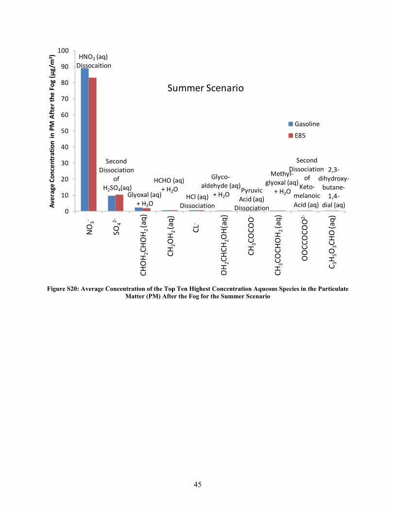
45

Figure S20: Average Concentration of the Top Ten Highest Concentration Aqueous Species in the Particulate

Matter (PM) After the Fog for the Summer Scenario

0

10

20

30

40

50

60

70

80

90

100

NO3m

SO4m

m

aCHO

H2CH

OH2

aCH2

OH2 CLm

aOH2

CHCH

2OH

CH3C

OCO

Om

aCH3

COCH

OH2

OOCC

OCO

Omm

aC3H

5O3C

HO

Average Co

ncen

tration in PM After th

e Fog (μg/m

3 )

Gasoline

E85

HNO3 (aq)Dissocaition

HCl (aq)Dissociation

Second Dissociation 

of H2SO4(aq)

Glyoxal (aq)+ H2O

HCHO (aq)+ H2O

SecondDissociation 

ofKeto‐

melanoicAcid (aq) 

2,3‐dihydroxy‐butane‐1,4‐

dial (aq)

Glyco‐aldehyde (aq)

+ H2O

Methyl‐glyoxal (aq)

+ H2OPyruvicAcid (aq)

Dissociation

Summer ScenarioNO

3‐

SO42‐

CL‐

CHOH2CHOH2 (aq)

CH2OH2 (aq)

OH2CHCH

2OH(aq)

CH3COCO

O‐

CH3COCH

OH2 (aq)

OOCC

OCO

O2‐

C 3H5O

3CHO(aq)

46

Figure S21: Average Concentration of the Top Ten Highest Concentration Aqueous Species in the Particulate

Matter (PM) After the Fog for the Winter Scenario

4. Model Sensitivity The sensitivity of the model results without a fog are discussed in Ginnebaugh et al. (2010). The sensitivity of the results to fog parameters is described in the main paper along with results for the summer scenario. The remaining results for the summer scenario and all results for the winter scenario are shown here (Figure S22, Figure S23, and Figure S24).

0

1

2

3

4

5

6

7

8

9

10

aCH2

OH2

NO3m

SO4m

m

aCHO

H2CH

OH2

aOH2

CHCH

2OH

aCH3

COCH

OH2

HMSm

HSO3m

CH3C

OCO

Om

aCH3

CHOH2

Average Co

ncen

tration in PM After th

e Fog (μg/m

3 )

Gasoline

E85

HNO3(aq)Dissocaition

SO2 (aq)+ H2O

PyruvicAcid (aq)

Dissociation

Second Dissociation 

of H2SO4(aq)

Glyoxal (aq)+ H2O

HCHO (aq)+ H2O

Glycoaldehyde (aq)+ H2O

Methylglyoxal (aq)+ H2O HSO3

‐

+ HCHO (aq) CH3CHO (aq)+ H2O

Winter Scenario

NO

3‐

SO42‐

CHOH2CHOH2 (aq)

CH2OH2 (aq)

OH2CHCH

2OH(aq)

CH3COCH

OH2(aq)

HMS‐

HSO

3‐

CH3COCO

O‐

CH3CHOH2 (aq)

47

Figure S22: Difference in Two Day Average Ozone Concentration (E85 – Gasoline) (top figure) and Two Day

Average Ozone Concentration for E85 and Gasoline (bottom figure) to Test the Model’s Sensitivity to Fog Parameters for the Summer Scenario

0

20

40

60

80

100

120

Fog

Smaller D

rop

Aerosol

Lower LW

C

Higher LW

C

Longer Duration Fog

Decreased Ph

otolysis

No Ph

otolysis Redu

ction (Fog)

No Ph

otolysis Redu

ction (Aerosol)

2 Da

y Av

g Ozone

 (g + a)  (ppb

)

GasolineE85

0

2

4

6

8Differen

ce (E85

 ‐Ga

soline) (pp

b)

Sensitivities

Summer Scenario

48

Figure S23: Difference in Two Day Average Ozone Concentration (E85 – Gasoline) (top figure) and Two Day

Average Ozone Concentration for E85 and Gasoline (bottom figure) to Test the Model’s Sensitivity to Fog Parameters for the Winter Scenario

0

5

10

15

Differen

ce (E85

 ‐Ga

soline) (pp

b)

0

5

10

15

20

25

30

Fog

Smaller D

rop

Aerosol

Lower LW

C

Higher LW

C

Longer Duration Fog

Decreased Ph

otolysis

No Ph

otolysis Redu

ction (Fog)

No Ph

otolysis Redu

ction (Aerosol)

2 Da

y Av

g Ozone

 (g+aq)  (pp

b)

Gasoline

E85

Sensitivities

Winter Scenario

49

Figure S24: Difference in Two Day Average Ozone (gas + aqueous) Concentration (Sensitivity – Baseline Fog Case) and Percent Change ((Sensitivity – Baseline Fog)/Baseline Fog) to Test the Model’s Sensitivity to Fog

Parameters for the Winter Scenario

5. Summary In this Supplemental Information, we have provided information on the emissions and model used for this study beyond that described in the main paper. We have shown that E85 may increase urban ozone over gasoline in a variety of scenarios. The increase is significantly greater at colder temperatures, implying a significant impact on human health during the winter when using E85. We also found that, under certain warm, summer conditions, a morning fog can increase afternoon ozone for both gasoline and E85.

‐6

‐4

‐2

0

2

4

6

8

Smaller Drop

Aerosol Lower LWC Higher LWC Longer Duration 

Fog

Decreased Photolysis

No Photolysis Reduction (Fog)

No Photolysis Reduction (Aerosol)

Differen

ce (Sen

sitivity

 ‐Ba

seline Fog) in

 Avg O

3Co

nc (p

pb)

Gasoilne

E85

Winter Scenario

0% 0%7%

23%

4%

17%

‐1% ‐2% ‐7%

‐24%

‐2%‐2% 2%3%

10%

29%

50

References AQMD. (2008). South Coast Air Basin Map. from http://www.aqmd.gov/map/MapAQMD1.pdf. Black, F (1995-1997). Characterization of Alternative Fuel Vehicle Emssions Composition and

Ozone Potential. EPA No. RW89936763 Annual Reports to the Department of Energy. Bloss, C, V Wagner, A Bonzanini, M E Jenkin, K Wirtz, M Martin-Reviejo and M J Pilling

(2005a). Evaluation of detailed aromatic mechanisms (MCMv3 and MCMv3.1) against environmental chamber data. Atmos. Chem. Phys. 5(3): 623-639.

Bloss, C, V Wagner, M E Jenkin, R Volkamer, W J Bloss, J D Lee, D E Heard, K Wirtz, M Martin-Reviejo, G Rea, J C Wenger and M J Pilling (2005b). Development of a detailed chemical mechanism (MCMv3.1) for the atmospheric oxidation of aromatic hydrocarbons. Atmos. Chem. Phys. 5(3): 641-664.

Brewer, R L, R J Gordon, L S Shepard and E C Ellis (1983). Chemistry of mist and fog from the Los Angeles urban area. Atmospheric Environment (1967) 17(11): 2267-2270. DOI: 10.1016/0004-6981(83)90224-x.

CARB. (2008). California Environmental Protection Agency Air Resources Board Real-Time Query Tool AQ2MIS. from http://www.arb.ca.gov/aqmis2/paqdselect.php.

Carter, W P L (2008). Development of an Improved Chemical Speciation Database for Processing Emissions of Volatile Organic Compounds for Air Quality Models, College of Engineering, Center for Environmental Research and Technology (CE-CERT), University of California, Riverside.

Derwent, R G, M E Jenkin, N R Passant and M J Pilling (2007). Photochemical ozone creation potentials (POCPs) for different emission sources of organic compounds under European conditions estimated with a Master Chemical Mechanism. Atmos. Environ. 41(12): 2570-2579.

Derwent, R G, M E Jenkin, S M Saunders, M J Pilling and N R Passant (2005). Multi-day ozone formation for alkenes and carbonyls investigated with a master chemical mechanism under European conditions. Atmos. Environ. 39(4): 627-635.

Derwent, R G, M E Jenkin, S M Saunders, M J Pilling, P G Simmonds, N R Passant, G J Dollard, P Dumitrean and A Kent (2003). Photochemical ozone formation in north west Europe and its control. Atmos. Environ. 37(14): 1983-1991.

EPA (2006). Clearinghouse for Inventories and Emission Factors, United States Environmental Protection Agency, Washington, D.C.

Ervens, B, C George, J E Williams, G V Buxton, G A Salmon, M Bydder, F Wilkinson, F Dentener, P Mirabel, R Wolke and H Herrmann (2003). CAPRAM 2.4 (MODAC mechanism): An extended and condensed tropospheric aqueous phase mechanism and its application. J. Geophys. Res. 108(D14). DOI: 10.1029/2002JD002202.

Evtyugina, M G, C Pio, T Nunes, P G Pinho and C S Costa (2007). Photochemical ozone formation at Portugal West Coast under sea breeze conditions as assessed by master chemical mechanism model. Atmos. Environ.

Ginnebaugh, D L, J Liang and M Z Jacobson (2010). Examining the temperature dependence of ethanol (E85) versus gasoline emissions on air pollution with a largely-explicit chemical mechanism. Atmos. Environ. 44: 1192-1199. DOI: 10.1016/j.atmosenv.2009.12.024.

Herrmann, H, B Ervens, P Nowacki, R Wolke and R Zellner (1999). A chemical aqueous phase radical mechanism for tropospheric chemistry. Chemosphere 38(6): 1223-1232.

51

Herrmann, H, A Tilgner, P Barzaghi, Z Majdik, S Gligorovski, L Poulain and A Monod (2005). Towards a more detailed description of tropospheric aqueous phase organic chemistry: CAPRAM 3.0. Atmos. Environ. 39(23-24): 4351-4363.

Hynes, R G, D E Angove, S M Saunders, V Haverd and M Azzi (2005). Evaluation of two MCM v3.1 alkene mechanisms using indoor environmental chamber data. Atmos. Environ. 39: 7251–7262.

Jacob, D J, J M Waldman, J W Munger and M R Hoffmann (1985). Chemical composition of fogwater collected along the California coast. Environ. Sci. Technol. 19(8): 730-736. DOI: 10.1021/es00138a013.

Jacobson, M Z (1995). Computation of Global Photochemistry with SMVGEAR II. Atmos. Environ. 29(18): 2541-2546.

Jacobson, M Z (1998). Improvement of SMVGEAR II on vector and scalar machines through absolute error tolerance control. Atmos. Environ. 32(4): 791-796.

Jacobson, M Z (2005). Fundamentals of Atmospheric Modeling. New York, Cambridge University Press. Second Edition.

Jacobson, M Z (2007). Effects of ethanol (E85) versus gasoline vehicles on cancer and mortality in the United States. Environ. Sci. Technol. 41(11): 4150-4157.

Jacobson, M Z and R P Turco (1994). SMVGEAR: A Sparse-Matrix, Vectorized Gear Code for Atmospheric Models. Atmos. Environ. 28(2): 273-284.

Jenkin, M E (2004). Modelling the formation and composition of secondary organic aerosol from a- and b-pinene ozonolysis using MCM v3. Atmos. Chem. Phys. Disscusions 4: 2905–2948.

Jenkin, M E, S M Saunders and M J Pilling (1997). The tropospheric degradation of volatile organic compounds: a protocol for mechanism development. Atmos. Environ. 31(1): 81-104.

Jenkin, M E, S M Saunders, V Wagner and M J Pilling (2003). Protocol for the development of the Master Chemical Mechanism, MCM v3 (Part B): tropospheric degradation of aromatic volatile organic compounds. Atmos. Chem. Phys. Disscusions 2: 1905–1938.

Johnson, D, M E Jenkin, K Wirtz and M Martin-Reviejo (2004). Simulating the Formation of Secondary Organic Aerosol from the Photooxidation of Toluene. Environ. Chem. 1(3): 150-165.

Johnson, D, M E Jenkin, K Wirtz and M Martin-Reviejo (2005). Simulating the Formation of Secondary Organic Aerosol from the Photooxidation of Aromatic Hydrocarbons. Environ. Chem. 2(1): 35-48.

Johnson, D, S R Utembe and M E Jenkin (2006a). Simulating the detailed chemical composition of secondary organic aerosol formed on a regional scale during the TORCH 2003 campaign in the southern UK. Atmos. Chem. Phys. 6(2): 419-431.

Johnson, D, S R Utembe, M E Jenkin, R G Derwent, G D Hayman, M R Alfarra, H Coe and G McFiggans (2006b). Simulating regional scale secondary organic aerosol formation during the TORCH 2003 campaign in the southern UK. Atmos. Chem. Phys. 6(2): 403-418.

Lurmann, F W, A S Wexler, S N Pandis, S Musarra, N Kumar and J H Seinfeld (1997). Modelling urban and regional aerosols—II. Application to California's South Coast Air Basin. Atmos. Environ. 31(17): 2695-2715. DOI: 10.1016/s1352-2310(97)00100-3.

MCM. University of LEEDS. (2002). Master Chemical Mechanism v. 3.1. from http://mcm.leeds.ac.uk/MCMv3.1/.

52

Munger, J W, J Collett Jr, B Daube Jr and M R Hoffmann (1990). Fogwater chemistry at Riverside, California. Atmospheric Environment. Part B. Urban Atmosphere 24(2): 185-205. DOI: 10.1016/0957-1272(90)90025-p.

Munger, J W, D J Jacob, J M Waldman and M R Hoffmann (1983). Fogwater chemistry in an urban atmosphere. J. Geophys. Res. 88(C9): 5109-5121. DOI: 10.1029/JC088iC09p05109.

Pilling, M J (2007). Representation of Chemical Detail in Atmospheric Models. Regional Climate Variability and its Impacts in The Mediterranean Area, Springer Netherlands. 79: 207-218.

Pinho, P, C Pio, W Carter and M Jenkin (2006a). Evaluation of alkene degradation in the detailed tropospheric chemistry mechanism, MCM v3, using environmental chamber data. J. Atmos. Chem. 55(1): 55-79.

Pinho, P G, C A Pio, W P L Carter and M E Jenkin (2007). Evaluation of α- and β-pinene degradation in the detailed tropospheric chemistry mechanism, MCM v3.1, using environmental chamber data. J. Atmos. Chem. 57(2): 171-202. DOI: 10.1007/s10874-007-9071-0.

Pinho, P G, C A Pio and M E Jenkin (2005). Evaluation of isoprene degradation in the detailed tropospheric chemical mechanism, MCM v3, using environmental chamber data. Atmos. Environ. 39(7): 1303-1322.

Pinho, P G, C A Pio and M E Jenkin (2006b). Evaluation of the Detailed Tropospheric Chemical Mechanism, MCM v3, Using Environmental Chamber Data: Butane and Its Degradation Products. Environmental Simulation Chambers: Application to Atmospheric Chemical Processes, Springer Netherlands. 62: 241-252.

Saunders, S M, M E Jenkin, R G Derwent and M J Pilling (2003). Protocol for the development of the Master Chemical Mechanism, MCM v3 (Part A): tropospheric degradation of non-aromatic volatile organic compounds. Atmos. Chem. Phys. 3: 161–180.

Tilgner, A and H Herrmann. Tilgner, A. and H. Herrmann. (2007). CAPRAM (= Chemical Aqueous Phase RAdical Mechanism). from http://projects.tropos.de/capram/index.html.

USEPA. (2000). Diurnal Profile File for CAIR - Emissions Modeling Clearinghouse Temporal Allocation. from http://www.epa.gov/ttn/chief/emch/temporal/.

Wagner, V, M E Jenkin, S M Saunders, J Stanton, K Wirtz and M J Pilling (2002). Modelling of the photooxidation of toluene: conceptual ideas for validating detailed mechanisms. Atmos. Chem. Phys. Disscusions 2: 1217–1259.

Waldman, J M, J W Munger, D J Jacob, R C Flagan, J J Morgan and M R Hoffmann (1982). Chemical composition of acid fog. Science 218(4573): 677-680. DOI: 10.1126/science.218.4573.677.

West, B H, A J López, T J Theiss, R L Graves, J M Storey and S A Lewis (2007). Fuel Economy and Emissions of the Ethanol-Optimized Saab 9-5 Biopower. 2007-01-3994 Oak Ridge National Laboratory.

Westerholm, R, P Ahlvik and H L Karlsson (2008). An exhaust characterisation study based on regulated and unregulated tailpipe and evaporative emissions from bi-fuel and flex-fuel light-duty passenger cars fuelled by petrol (E5), bioethanol (E70, E85) and biogas tested at ambient tempeatures of + 22C and -7C. Swedish Road Administration.

Whitney, K and T Fernandez (2007). Characterization of cold temperature VOC and PM emissions from flex fuel vehicles operating on ethanol blends. 17th CRC On-Road Vehicle Emissions Workshop.

53

Zador, J, V Wagner, K Wirtz and M J Pilling (2005). Quantitative assessment of uncertainties for a model of tropospheric ethene oxidation using the European Photoreactor (EUPHORE). Atmos. Environ. 39(15): 2805-2817.