Embed Size (px)
Citation preview
1
Supporting Information
Equation-free Mechanistic Ecosystem Forecasting Using Empirical Dynamic
Modeling
Hao Ye1, Richard J. Beamish2, Sarah M. Glaser3, Sue. C.H. Grant4, Chih-hao Hsieh5, Laura J.
Richards2, Jon T. Schnute2, and George Sugihara1 1 Scripps Institution of Oceanography, University of California, San Diego, La Jolla, CA 92093 2 Pacific Biological Station, Fisheries and Oceans Canada, Nanaimo, BC V9T 6N7, Canada 3 Joseph S. Korbel School of International Studies, University of Denver, Denver, CO 80210 4 Fisheries and Oceans Canada, Delta, BC V3M 6A2, Canada 5 Institute of Oceanography and Institute of Ecology and Evolutionary Biology, National Taiwan
University, Taipei, Taiwan, 10617
Corresponding Authors:
Hao Ye and George Sugihara
9500 Gilman Drive MC0208
La Jolla, CA, USA 92093-0208
(858) - 534 - 5582
2
Supplementary Text
Attractor Reconstruction from Time Series
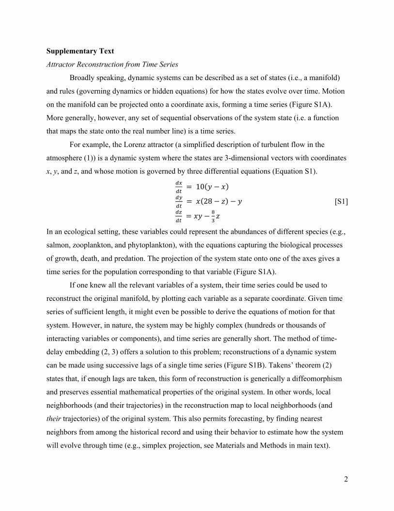
Broadly speaking, dynamic systems can be described as a set of states (i.e., a manifold)
and rules (governing dynamics or hidden equations) for how the states evolve over time. Motion
on the manifold can be projected onto a coordinate axis, forming a time series (Figure S1A).
More generally, however, any set of sequential observations of the system state (i.e. a function
that maps the state onto the real number line) is a time series.
For example, the Lorenz attractor (a simplified description of turbulent flow in the
atmosphere (1)) is a dynamic system where the states are 3-dimensional vectors with coordinates
x, y, and z, and whose motion is governed by three differential equations (Equation S1).
!"!" != !10 ! − !!"!" != !! 28− ! − !!"!" != !" − !
! ! [S1]
In an ecological setting, these variables could represent the abundances of different species (e.g.,
salmon, zooplankton, and phytoplankton), with the equations capturing the biological processes
of growth, death, and predation. The projection of the system state onto one of the axes gives a
time series for the population corresponding to that variable (Figure S1A).
If one knew all the relevant variables of a system, their time series could be used to
reconstruct the original manifold, by plotting each variable as a separate coordinate. Given time
series of sufficient length, it might even be possible to derive the equations of motion for that
system. However, in nature, the system may be highly complex (hundreds or thousands of
interacting variables or components), and time series are generally short. The method of time-
delay embedding (2, 3) offers a solution to this problem; reconstructions of a dynamic system
can be made using successive lags of a single time series (Figure S1B). Takens’ theorem (2)
states that, if enough lags are taken, this form of reconstruction is generically a diffeomorphism
and preserves essential mathematical properties of the original system. In other words, local
neighborhoods (and their trajectories) in the reconstruction map to local neighborhoods (and
their trajectories) of the original system. This also permits forecasting, by finding nearest
neighbors from among the historical record and using their behavior to estimate how the system
will evolve through time (e.g., simplex projection, see Materials and Methods in main text).

3
Identifying Nonlinearity in Sockeye Salmon Dynamics
One application of EDM is to identify nonlinear dynamics in time series. For the Fraser
River system, we first consider the 9 stocks in aggregate. Following (4), each time series of
returns is linearly transformed to have mean = 0 and variance = 1. This preserves the quasicyclic
behavior of each stock, but corrects for the relative magnitude across different stocks. The
normalized time series are joined together end-to-end, in effect treating them as 9 instances of a
single time series. Using simplex projection with τ = 1 and predicting 1 year into the future,
forecast skill (ρ) is maximized when 4 successive lags are used (Figure S2A). This is somewhat
expected, because the quasi-cyclic nature of these returns has a 4 year periodicity: knowing the
previous 4 years is sufficient to identify the current phase and estimate the current magnitude of
returns.
Next, we employ the S-map procedure (5), which compares equivalent linear and
nonlinear models (adjusting a tuning parameter, θ) to test for nonlinear dynamics. When θ = 0,
all points are weighted equally, and the model reduces to an autoregressive model of order E. For
θ > 0, nearby points are given stronger weighting, allowing the model to be adaptive to local
influences and therefore, nonlinear. If the behavior of sockeye returns is purely periodic, then the
linear model should have the highest forecast skill, because it can smooth out errors over the
entire data set. However, Figure S2B shows that forecast skill peaks when θ is ~ 2, which is
evidence for nonlinearity in the aggregate time series. Using the randomization test of (6, 7), this
improvement in forecast skill (decrease in MAE) is significant with P = 0.002.
As noted in (4), nonlinearity may appear as an artifact when aggregating linear time
series with somewhat different dynamics. Therefore, to confirm the presence of nonlinearity, we
also apply the S-map to each stock individually, using the same randomization test for whether
the improvement in forecast error (MAE) is significant at the α = 0.10 level (Table S1). Overall,
these results are encouraging: we find 6 of the 9 stocks to be significantly nonlinear. We note,
however, that the lack of significant nonlinearity in the Birkenhead, Seymour, and Weaver stocks
may not necessarily indicate that these stocks are linear, as the S-map test can require lengthy
time series for accurate discrimination.
Convergent Cross Mapping
If salmon mortality is strongly influenced by the environment, then the time series of
salmon recruitment will contain information about past environmental states. This means that it

4
is possible to estimate past environmental conditions from salmon abundances. To the extent that
this is true, the ability to recover past environmental states from the salmon time series is
evidence for causal influence by the environment. This criterion for causation (convergent cross
mapping, CCM) can be used to identify key variables and operates in nonlinear systems whereas
linear correlation does not (8, 9).
CCM operates on much the same principle as generalized simplex projection in Equation
2 (see Materials and Methods in main text). Here, the notion is that if variable y has a causal
influence on x, then the system state (represented using only lags of x) will contain an imprint of
y. Thus, it should be possible to map between states of the system (the univariate reconstruction
based on x) and the value of y. Cross mapping strength can be assessed by the correlation
between the estimated values of y and the corresponding observed values. In a fully deterministic
system with no noise, we expect this cross mapping correlation to approach 1 as time series
length increases and the reconstruction becomes denser. As a practical indicator of causal
influence, here we test whether the correlation is significantly positive when using the whole
time series.
It is important to note that if a variable y is stochastic and influences x with a time lag,
then cross mapping from x to y may show evidence of a causal interaction only if the
appropriately lagged value of y is estimated. Here, we are interested in testing for the influence
of the environment on juvenile salmon, which occurs when the salmon are 2 years old. Thus, a
reconstruction based on salmon abundance for brood year t should be informative about the
environment in calendar year t+2. Moreover, because it is only the 2-year old salmon that are
affected by this early oceanic environment, it would not make sense to include measures of
salmon abundance from multiple spawning broods (i.e., only salmon from brood year t should
have information about the environment in year t+2). Therefore, we use multivariate CCM, cross
mapping from the reconstruction !! = !!!,!!! (where !!! and !!! are the cycle-line normalized
spawner and recruit abundances of brood year t, respectively, to account for the effect of cyclic
dominance) to yt = Ut+2 (where Ut+2 is an environmental variable measured in calendar year t+2),
to estimate the environmental effect that would have influenced that brood of salmon.
Table S3 shows the cross mapping results for each combination of the 9 stocks and 12
environmental time series considered in this work. Only some of the relationships appear
significant, with most of the significant cross mapping occurring between temperature and the

5
Chilko, Early Stuart, Late Stuart, and Quesnel stocks. Surprisingly, this did not seem to match
well with the identification of environmental variables using multivariate EDM (SST does not
appear to be a necessary variable to achieve skillful forecasts for Chilko, Early Stuart, or Late
Stuart). Moreover, for some stocks, river discharge or the PDO appeared to be important (EDM
models excluding those variables produced substantially less accurate forecasts). Overall, this
suggests that the effects of these environmental variables on recruitment may be more complex
than can be captured with our CCM analysis. For instance, it could be the case that knowing the
spawner abundance and river discharge can predict recruitment, but that this function may not be
one-to-one, and so it is difficult to cross map the historical river discharge from the spawner and
recruit data of a specific brood year.
In other systems, we could resolve such singularities in the cross mapping relationship by
including more coordinates (i.e., using additional time series lags) in the reconstruction.
However, here we are limited by the fact that our data (generally) record only 2 measurements of
abundance for each spawning brood (spawner abundance and recruitment). Such is not the case
for other marine species that are sampled in annual surveys, where an external influence that has
occurred at a particular life stage will leave a record multiple times in the data (because the
affected organisms will be recorded in many consecutive data points).
Determining Causal Environmental Variables
In addition to improving forecasts, an important application of EDM is to identify
informative environmental variables and elucidate potential mechanisms. Here, an environmental
variable is deemed causal if including that variable into a multivariate EDM model improves
forecast skill. Thus, we use multivariate EDM to determine if the environment has any causal
influence on sockeye salmon recruitment, by testing different combinations of environmental
variables (Table S4). As noted above, data limitations mean that the CCM analysis (Table S3)
may not be sensitive enough to identify environmental drivers for this system.
The results of multivariate EDM (Table S4) reveal which specific variables may be
uniquely informative for particular stocks, or whether some variables may actually be
interchangeable. When interpreting Table S4, it is important to keep in mind the nonuniqueness
property of EDM models (i.e., there is no “true” model, but many combinations of variables that
can give similarly good performance). Thus, the inclusion of a variable in multivariate EDM
does not imply a direct causal link, as the variable could be an indirect observation of the true

6
mechanism. Furthermore, the exclusion of a variable does not mean that said variable has no
effect, either. It could be the case that multiple stochastic drivers interact to affect recruitment,
such that an incomplete set of observations on those drivers do not improve forecasts. In such
cases, extending the set of tested variables may reveal causal mechanisms that were previously
hidden.
In addition, because EDM operates in a nonlinear (non-additive) framework, we note that
it is not possible to partition a model’s performance (i.e., variance explained) in terms of
individual variables. Nonlinear state-dependence necessarily implies that the effect of one
variable may depend on another. For example, in a model that includes temperature and river
discharge, the addition of temperature may improve forecasts only under certain conditions of
river discharge (e.g., low temperatures are better for recruitment, but only when river discharge
is high). Including temperature by itself may not improve forecasts at all, and so the “variance
explained” by temperature necessarily depends on the other variables of the EDM model, thus
making it impossible to assign independent r2 (variance explained) values for each variable in the
model.
Possible Causal Mechanisms for SST, River Discharge, and the PDO
The tested variables (river discharge, sea-surface temperature, the Pacific Decadal
Oscillation) have been thought to influence sockeye salmon recruitment by being indicative of
juvenile mortality in the early marine period (i.e., the first year of ocean residence) (10). For
example, river discharge may improve multivariate EDM forecasts because of its effect on food
availability, which is believed to play a role in determining this mortality (11). By affecting
estuarine circulation in the Strait of Georgia, freshwater input (from the Fraser River and other
riverine sources) can influence ocean productivity (12); indeed, river discharge, in combination
with wind and other factors, has been linked to low oceanic productivity in the Strait of Georgia
that may have contributed to poor returns of sockeye salmon in 2009 (11, 13).
Using multivariate EDM, we do find support for river discharge as an informative
variable, with the best EDM model for 4 of the 9 stocks containing river discharge as a
coordinate (Table 1). Furthermore, for these 4 stocks (Early Stuart, Late Shuswap, Late Stuart,
and Weaver), nearly all of the top-ranking EDM models include river discharge as a coordinate
(i.e., Table S4). However, other than Late Stuart, there are EDM models excluding river
discharge that have similar performance, suggesting that for Early Stuart, Late Shuswap, and

7
Weaver, river discharge may be redundant if other observations of the environmental are
available. Thus, while river discharge may be an informative variable, it does not appear to be
strictly necessary for skillful predictions, except in the case of Late Stuart.
Pine Island SST also appears to be an important variable, and is included in the best
multivariate model for 4 of the 9 stocks (Table 1). With Pine Island lighthouse located at the
boundary between Queen Charlotte Strait and Queen Charlotte Sound (Figure 3), the measured
SST could be informative about the conditions that juvenile sockeye salmon experience after
exiting the Strait of Georgia. That Pine Island SST can be informative about recruitment
resonates with evidence that anomalous conditions in this area during 2007 were associated with
low returns 2 years later (2009), while favorable conditions (low freshwater runoff and moderate
northerly winds) in 2008 were associated with record high returns in 2010 (13). Here, only the
Quesnel stock seems to require Pine Island SST for skillful forecasts, as the best model for
Quesnel excluding this variable is much less skillful. For the remaining 3 stocks where the best
EDM model included Pine Island SST, there were alternative multivariate EDM models
including only other variables that showed very similar performance (Table S4). This suggests
that the information in Pine Island SST relevant for predicting recruitment in these stocks may be
duplicated in other environmental variables (see discussion in main text on non-uniqueness).
Lastly, although many studies (14-16) have found that decadal-scale climate and oceanic
indicators, such as the PDO, are predictive of regional productivity for Pacific salmon, one
important question is whether this relationship holds at the individual stock level (i.e., do all
stocks rise and fall in sync with one another). Among the Fraser River sockeye salmon, at least,
there do not appear to be consistent patterns: there has been an overall decline since the early
1990s, but productivity for some stocks (e.g., Early Stuart) has been declining since the 1960s,
while others (e.g., Late Shuswap, Weaver) have not exhibited a declining trend at all (17). Our
results similarly show no uniform effect of the PDO, as the best EDM model only includes the
PDO as a coordinate for 2 of 9 stocks. In both cases (Stellako and Quesnel), however,
performance is substantially improved when other variables are included compared to the model
that includes just the PDO (Table S4). Thus, while the PDO may be informative for overall
productivity of the Fraser River system, individual stocks appear to be sensitive to more
localized environmental conditions; thus including additional (local) environmental variables is
essential for improving forecasts for those stocks.

8
Including Smolt Data into EDM Models
For the Chilko stock, even an exhaustive search for the best possible multivariate EDM
model did not produce very accurate forecasts (ρ < 0.4, Figure S4). One possible explanation is
that the relationship between spawner abundance and recruits is complex, such that a
reconstruction using spawning stock and the tested environmental variables does not uniquely
determine recruitment. In such cases, additional observations, such as other environmental
factors or measures of salmon abundance at different ages, could resolve singularities in the
reconstruction, thereby improving forecasts. For the Chilko stock, a long time series of smolt
abundance is available, allowing us to include this variable as an additional coordinate in the
multivariate EDM model (Equation S2, !!! is smolt abundance normalized to the current cycle
line). Testing this model, we found improvements in both accuracy and error (Figure S4).
!! = !!!, !!!,ET!!!,May,PDO!!! [S2]
Although the added expense of collecting this kind of data many not be reasonable for all
stocks (particularly those that are already very predictable using the tested variables), these
observations of sockeye at different ages are additional sources of information that could
potentially improve forecasts, giving managers the ability to make trade-offs between data
collection and predictability.
Estimating Uncertainty for Simplex Projection Forecasts
We note that the EDM models presented here produce point estimates for the number of
returning sockeye salmon. However, fisheries management protocols often require an estimate of
the uncertainty surrounding each forecast (i.e. confidence intervals) in order to evaluate the risks
associated with management actions. Within the EDM framework, this uncertainty can be
addressed in several ways. For example, the relative divergence of nearby trajectories in the
reconstructed state space measures how sensitive the future will be to the current state, and is
therefore directly indicative of forecast uncertainty. Here we demonstrate a simple
implementation of this idea, by noting that the simplex projection method produces forecasts by
computing a weighted average of the target variable, y (equation 2 from the main text):
!!!! =!!(!)!! !,! !!
!!!!
!!(!)!!!!
[S3]
In effect, the values of yn(s,i)+h can be thought of as the sample space for the desired prediction,
where each value has probability !! ! = !! !!! !!
!!!. Equation S3 computes a forecast as the

9
expected value of this probability mass function. This idea can then be extended to the second
moment of this function in order to compute a variance:
Var !!!! = E (!! !,! !! − !!!!)! = !! ! !! !,! !!!!!!!!!
!!!!!(!)!
!!! [S3]
Note that as the difference between each neighbor’s forecast and the weighted average increases,
variance will also increase, thus tracking the divergence of the nearest neighbors.
Because simplex projection is used to forecast relative age 4 and age 5 recruits, which are
linearly combined to forecast returns (see Materials and Methods), we can similarly compute the
variance of returns:
Var !! = Var !!,!!! + Var !!,!!! + Cov(!!,!!!,!!,!!!)
Var !!.! = Var !!,!! ∙ !! !!! [S4]
Here, because the age 4 and age 5 recruits are computed from separate data, we can assume that
the covariance is 0 (because the selection of nearest neighbors used to compute !!,!!! are
independent of those used to compute !!,!!!).
This is demonstrated in Figure S5 for the best multivariate EDM model of the Late
Shuswap stock. Plotting the EDM forecasts along with standard errors, it is clear that there is
good correspondence: variability is higher for the dominant cycle line (as would be expected)
and forecasts are generally within 1 standard error of the realized returns.

10
SI References
1. Lorenz EN (1963) Deterministic nonperiodic flow. Journal of the Atmospheric Sciences
20: 130-141.
2. Takens F (1981) Detecting strange attractors in turbulence. Dynamical Systems and
Turbulence, Lecture Notes in Mathematics 898: 366–381.
3. Crutchfield JP, McNamara BS (1987) Equations of motion from a data series. Complex
Systems 1: 417-52.
4. Hsieh CH, Anderson C, Sugihara G (2008) Extending nonlinear analysis to short
ecological time series. The American Naturalist 171:71-80.
5. Sugihara G (1994) Nonlinear forecasting for the classification of natural time series.
Philosophical Transactions: Physical Sciences and Engineering 348: 477–495.
6. Hsieh CH, Ohman MD (2006) Biological responses to environmental forcing: The linear
tracking window hypothesis. Ecology 87: 1932-1938.
7. Glaser SM, Fogarty MJ, Liu H, Hsieh CH, Kaufman L, et al. (2014) Complex dynamics
may limit prediction in marine fisheries. Fish and Fisheries 15: 616-33.
8. Sugihara G, May R, Ye H, Hsieh CH, Deyle E, et al. (2012) Detecting causality in
complex ecosystems. Science 338: 496-500.
9. Deyle ER, Fogarty M, Hsieh CH, Kaufman L, MacCall AD, et al. (2013) Predicting
climate effects on Pacific sardine. Proceedings of the National Academy of Sciences 110:
6430-6435.
10. Beamish RJ, Mahnken C, Neville CM (2004) Evidence that reduced early marine growth
is associated with lower marine survival of coho salmon. Transactions of the American
Fisheries Society 133: 26-33.
11. Beamish RJ, Neville C, Sweeting R, Lange K (2012) The synchronous failure of juvenile
Pacific salmon and herring production in the Strait of Georgia in 2007 and the poor return
of sockeye salmon to the Fraser River in 2009. Marine and Coastal Fisheries: Dynamics,
Management, and Ecosystem Science 4: 403-414.
12. Beamish RJ, Neville CEM, Thomson BL, Harrison PJ, John MS (1994) A relationship
between Fraser River discharge and interannual production of Pacific salmon
(Oncorhynchus spp.) and Pacific herring (Clupea pallasi) in the Strait of Georgia.
Canadian Journal of Fisheries and Aquatic Sciences 51: 2843-2855.

11
13. Thomson RE, Beamish RJ, Beacham TD, Trudel M, Whitfield PH, et al. (2012)
Anomalous ocean conditions may explain the recent extreme variability in Fraser River
sockeye salmon production. Marine and Coastal Fisheries: Dynamics, Management, and
Ecosystem Science 4: 415-437.
14. Mantua N, Hare S, Zhang Y, Wallace J (1997) A Pacific interdecadal climate oscillation
with impacts on salmon production. Bulletin of the American Meteorological Society 78:
1069–1079.
15. Beamish RJ, Neville CEM, Cass AJ (1997) Production of Fraser River sockeye salmon
(Oncorhynchus nerka) in relation to decadal-scale changes in the climate and the ocean.
Canadian Journal of Fisheries and Aquatic Sciences 54: 543-554.
16. Beamish RJ, Schnute JT, Cass AJ, Neville CM, Sweeting RM (2004) The influence of
climate on the stock and recruitment of pink and sockeye salmon from the Fraser River,
British Columbia, Canada. Transactions of the American Fisheries Society 133: 1395-
1412.
17. Grant SCH, Michielsens CGJ, Porszt EJ, Cass A (2010) Pre-season run size forecasts for
Fraser River sockeye salmon (Oncorhynchus nerka) 2010. DFO Canadian Science
Advisory Secretariat Research Document 2010/042.

12
Movie S1 (legend only)
This movie describes the essential mechanics of Empirical Dynamic Modeling, demonstrating the relationship between time series and dynamic attractors and illustrating how Takens’ Theorem (23) can be used to reconstruct a shadow manifold.

13
Figure S1. Reconstruction of System Dynamics from a Time Series
A Projecting the motion of the canonical Lorenz attractor onto the x-axis yields a time series for
variable x. B Successive lags (with time step τ) of the time series xt are plotted as separate
coordinates to form a reconstructed “shadow” manifold that preserves essential mathematical
properties of the original system (and is visually similar).
time
X
YZ
Xt
Xt-Ѭ
Xt-2Ѭ
IJ
2IJ
time
xt
Xt-2Ѭ
Xt
Xt-Ѭ
A
B
t

14
Figure S2. Nonlinearity in Fraser River Sockeye Salmon.
Following (36), we concatenate time series of returns for 9 stocks. A Forecasting returns using
simplex projection, 4 is identified as the optimal embedding dimension. B Using the S-map
procedure, forecast skill is highest for θ ~ 2 (P = 0.002), which demonstrates nonlinear state
dependence in salmon dynamics.
1 2 3 4 5 6
0.0
0.2
0.4
0.6
E
Fore
cast
Acc
urac
y (ѩ
)
Fore
cast
Pre
cisi
on (1
- M
AE)
A B
ѡ0 1 2 3 4
0.44
0.46
0.48
15
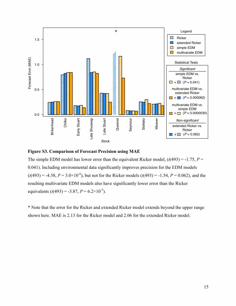
Figure S3. Comparison of Forecast Precision using MAE
The simple EDM model has lower error than the equivalent Ricker model, (t(493) = -1.75, P =
0.041). Including environmental data significantly improves precision for the EDM models
(t(493) = -4.58, P = 3.0×10⁻⁶), but not for the Ricker models (t(493) = -1.54, P = 0.062), and the
resulting multivariate EDM models also have significantly lower error than the Ricker
equivalents (t(493) = -3.87, P = 6.2×10⁻⁵).
* Note that the error for the Ricker and extended Ricker model extends beyond the upper range
shown here. MAE is 2.13 for the Ricker model and 2.06 for the extended Ricker model.
Birk
enhe
ad
Chi
lko
Early
Stu
art
Late
Shu
swap
Late
Stu
art
Que
snel
Seym
our
Stel
lako
Wea
ver
Fore
cast
Erro
r (M
AE)
Rickerextended Rickersimple EDMmultivariate EDM
Legend
Stock
Statistical Tests
multivariate EDM vs. extended Ricker
simple EDM vs. Ricker
multivariate EDM vs. simple EDM
extended Ricker vs. Ricker
Significant
Non-significant
< (P = 0.041)
≮ (P = 0.062)
< (P = 0.000062)
< (P = 0.0000030)0.0
0.5
1.0
1.5
�

16
Figure S4. Including Smolt Data into the Chilko EDM Model
For the Chilko stock, adding smolt time series as a coordinate in the best environmental EDM
model (spawners & May Entrance Island SST & the PDO) improves both accuracy and error.
0.0
0.1
0.2
0.3
0.4
0.5sp
awne
rs
+ en
viro
nmen
t
+ en
viro
nmen
t &
smol
ts
Data Usage
Fore
cast
Acc
urDF\��ѩ�
0.5
0.6
0.7
0.8
0.9
spaw
ners
+ en
viro
nmen
t
+ en
viro
nmen
t &
smol
ts
Fore
cast
Erro
r (M
AE, x
106 �

17
Figure S5. Standard Errors for EDM Forecasts of Late Shuswap Returns.
Extending the simplex projection algorithm, standard errors for each forecast can be computed.
Here, the predictions of the multivariate EDM model are plotted against observations for the
Late Shuswap stock.
1950 1960 1970 1980 1990 2000 2010
05
1015
Year
Retu
rns
(milli
ons
of fi
sh)
●
●
●
●●
●
●
●●
●
●
●●
●
●
●●
●
●
●●
●
●
●●
●
●●●
●
●
●●
●
●
●●
●
●
●●
●
●
●●
●
●
●●
●
●
●●
●
●
●●
●
ObservedPredicted (+/− 1 SE)

18
Table S1. Nonlinearity Tests for Individual Stocks
stock E θ ΔMAE P value significantly nonlinear?
Birkenhead 5 0 0 0.494 no Chilko 6 2 -0.070 *0.024 yes Early Stuart 6 4 -0.023 *0.050 yes Late Shuswap 4 2 -0.389 *0.014 yes Late Stuart 8 3 -0.054 *0.060 yes Quesnel 7 4 -0.298 *0.008 yes Seymour 8 0.5 -0.002 0.162 no Stellako 7 2 -0.025 *0.014 yes Weaver 1 0 0 0.496 no
E is embedding dimension, θ is the optimal value of the nonlinear tuning parameter, ΔMAE is
the difference in error between the model at the optimal value of θ and the model at θ = 0
(negative values indicate a decrease in error, or improvement with θ > 0), P value is for a
randomization test with 500 iterations (* indicates significance at the α = 0.10 level).

19
Table S2. Comparison of Model Performance
comparison performance measure
test type test statistic
df P value
simple EDM vs. Ricker
ρ t 1.77 492 *0.039 MAE t -1.75 493 *0.041
multivariate EDM vs. extended Ricker
ρ t 2.20 492 *0.014 MAE t -3.87 493 *6.2×10-5
extended Ricker vs. Ricker
ρ t 1.26 492 0.10 MAE t -1.54 493 0.062
multivariate EDM vs. simple EDM
ρ t 2.83 492 *0.0024 MAE t -4.58 493 *3.0×10-6
* indicates significance at the α = 0.05 level

20
Table S3. Results of Cross Mapping
N is the number of predictions, 95% ρ is the critical value for significance at the α = 0.05 level, “xmap {VAR}” columns are the cross
mapping correlations for {VAR}, where ET is Entrance Island SST, PT is Pine Island SST, D is Fraser River discharge, and PDO is
Pacific Decadal Oscillation. Highlighted cells indicate significant cross mapping at the α = 0.05 level.
stock N 95% ρ xmap Dmax
xmap Dapr
xmap Dmay
xmap Djun
xmap ETapr
xmap ETmay
xmap ETjun
xmap PTapr
xmap PTmay
xmap PTjun
xmap PTjul
xmap PDO
Birkenhead 58 0.218 0.108 -0.294 0.105 0.182 0.141 -0.122 0.046 -0.13 -0.003 0.029 -0.024 -0.151 Chilko 58 0.218 -0.197 0.045 0.172 -0.085 0.161 -0.024 0.215 0.244 0.194 0.288 0.211 0.042 Early Stuart 58 0.218 -0.005 -0.015 0.166 0.054 0.468 0.459 0.107 0.276 0.300 0.275 0.255 -0.079 Late Shuswap 58 0.218 -0.3 0.034 -0.178 -0.178 -0.081 0.309 0.011 0.024 0.018 0.166 0.199 0.192 Late Stuart 57 0.220 0.007 0.036 -0.058 -0.023 0.481 0.512 0.442 0.313 0.377 0.313 0.242 0.182 Quesnel 58 0.218 0.107 0.443 -0.033 0.087 0.599 0.371 0.243 0.523 0.611 0.562 0.532 0.2 Seymour 58 0.218 -0.326 0.006 0.157 -0.212 0.057 -0.185 -0.279 0.093 -0.073 0.069 0.219 0.230 Stellako 58 0.218 -0.063 0.085 -0.017 0.032 0.207 0.033 -0.298 0.101 0.032 0.123 0.081 -0.055 Weaver 40 0.264 -0.076 0.122 -0.285 0.044 -0.116 -0.213 -0.067 -0.286 -0.085 -0.068 0.043 -0.125

21
Table S4. Results of Multivariate EDM
stock predictors # predictions ρ MAE
Birkenhead
S 57 0.156 0.259 S, PTjul 57 0.125 0.26 S, Dmay 57 0.088 0.234 S, ETmay 57 0.005 0.282 S, PDO 57 0.005 0.293 S, PTmay 57 -0.022 0.319 S, Dmax 57 -0.034 0.303 S, ETjun 57 -0.108 0.287 S, PTjun 57 -0.119 0.324 S, Dapr 57 -0.144 0.306 S, Djun 57 -0.154 0.324 S, PTapr 57 -0.166 0.329 S, ETapr 57 -0.244 0.312
Chilko
S 57 0.264 0.839 S, PTjul 57 0.25 0.853 S, ETjun 57 0.221 1.006 S, Dmax 57 0.221 0.914 S, ETmay 57 0.208 0.942 S, PTmay 57 0.203 0.918 S, ETapr 57 0.199 0.934 S, PTapr 57 0.184 0.879 S, Dmay 57 0.177 0.839 S, PTjun 57 0.173 0.921 S, Dapr 57 0.153 0.896 S, PDO 57 0.065 1.014 S, Djun 57 -0.017 1.118
ET = Entrance Island SST, PT = Pine Island SST,
D = Fraser River discharge, PDO = Pacific Decadal Oscillation

22
Table S4. Results of Multivariate EDM (continued)
stock predictors # predictions
ρ MAE
Early Stuart
S, Dapr, Djun 57 0.878 0.140 S, Dmay, Djun 57 0.876 0.132 S, Djun, ETmay
57 0.858 0.132
S, Djun, PTjul 57 0.838 0.127 S, Djun, ETapr 57 0.837 0.131 S, Dmax, Djun 57 0.831 0.147 S, Djun, PTmay 57 0.830 0.144 S, Djun 57 0.830 0.134 S, ETapr 57 0.827 0.130 S, ETmay 57 0.824 0.137 S, Dmax 57 0.809 0.159 S, Djun, PTapr 57 0.803 0.156 S, Dmay 57 0.801 0.154 S, Djun, PDO 57 0.801 0.143 S, Djun, ETjun 57 0.794 0.159 S, Djun, PTjun 57 0.790 0.158 S, PTapr 57 0.789 0.157 S, ETjun 57 0.788 0.155 S, PTmay 57 0.787 0.165 S, PDO 57 0.783 0.151 S, PTjun 57 0.781 0.167 S, PTjul 57 0.749 0.172 S, Dapr 57 0.718 0.175 S 57 0.685 0.182
ET = Entrance Island SST, PT = Pine Island SST,
D = Fraser River discharge, PDO = Pacific Decadal Oscillation

23
Table S4. Results of Multivariate EDM (continued)
stock predictors # predictions ρ MAE
Late Shuswap
S, Dmay, PTjul 57 0.923 0.821 S, Dmay 57 0.912 0.807 S 57 0.900 0.852 S, Dmay, ETapr 57 0.892 0.918 S, Dmay, ETjun 57 0.862 0.968 S, Dmax 57 0.840 1.000 S, Dmay, PTmay 57 0.831 1.065 S, Dmay, ETmay 57 0.831 0.887 S, Dmay, Djun 57 0.819 1.079 S, Dapr 57 0.816 1.106 S, Dmay, PDO 57 0.801 1.161 S, PTjul 57 0.800 1.059 S, Dmax, Dmay 57 0.799 1.098 S, PDO 57 0.799 1.049 S, PTjun 57 0.795 1.197 S, PTmay 57 0.795 1.200 S, Dmay, PTapr 57 0.793 1.114 S, Dapr, Dmay 57 0.792 1.201 S, ETapr 57 0.784 1.115 S, ETmay 57 0.775 1.021 S, Dmay, PTjun 57 0.772 1.224 S, ETjun 57 0.764 1.203 S, PTapr 57 0.753 1.206 S, Djun 57 0.739 1.200
ET = Entrance Island SST, PT = Pine Island SST,
D = Fraser River discharge, PDO = Pacific Decadal Oscillation

24
Table S4. Results of Multivariate EDM (continued)
stock predictors # predictions ρ MAE
Late Stuart
S, Djun, ETapr 56 0.783 0.250 S, Dmay, Djun 56 0.752 0.305 S, Dapr, Djun 56 0.733 0.300 S, Djun, PTjul 56 0.708 0.316 S, Djun 56 0.706 0.319 S, ETmay 56 0.675 0.344 S, Dmax, Djun 56 0.667 0.343 S, Djun, PDO 56 0.644 0.338 S, ETapr 56 0.638 0.336 S, Djun, PTmay 56 0.625 0.348 S, Djun, ETjun 56 0.625 0.362 S, Djun, ETmay 56 0.621 0.365 S, Djun, PTapr 56 0.618 0.352 S, PTjun 56 0.602 0.403 S, Dmay 56 0.590 0.376 S, Dapr 56 0.588 0.409 S 56 0.550 0.422 S, PTmay 56 0.548 0.414 S, Djun, PTjun 56 0.548 0.394 S, PTapr 56 0.545 0.430 S, PDO 56 0.545 0.368 S, PTjul 56 0.518 0.418 S, ETjun 56 0.509 0.428 S, Dmax 56 0.469 0.478
ET = Entrance Island SST, PT = Pine Island SST,
D = Fraser River discharge, PDO = Pacific Decadal Oscillation

25
Table S4. Results of Multivariate EDM (continued)
stock predictors # predictions ρ MAE
Quesnel
S, PTmay, PDO 57 0.861 0.729 S, ETjun, PTmay 57 0.787 0.871 S, PTapr, PTmay 57 0.770 0.894 S, Djun, PTmay 57 0.768 0.895 S, Dmax, PTmay 57 0.756 0.884 S, ETapr, PTmay 57 0.754 0.922 S, PTmay 57 0.753 0.889 S, PTmay, PTjul 57 0.739 0.905 S, PTapr 57 0.729 0.969 S, PTmay, PTjun 57 0.726 0.945 S, Djun 57 0.724 0.927 S, Dmax 57 0.705 0.942 S, PDO 57 0.697 0.950 S, ETjun 57 0.674 1.133 S, Dmay, PTmay 57 0.651 1.048 S, ETmay, PTmay 57 0.642 1.071 S, ETapr 57 0.616 1.121 S, Dapr, PTmay 57 0.589 1.068 S, PTjun 57 0.571 1.087 S, PTjul 57 0.569 1.164 S 57 0.569 1.168 S, Dapr 57 0.500 1.297 S, ETmay 57 0.476 1.358 S, Dmay 57 0.459 1.311
ET = Entrance Island SST, PT = Pine Island SST,
D = Fraser River discharge, PDO = Pacific Decadal Oscillation

26
Table S4. Results of Multivariate EDM (continued)
ET = Entrance Island SST, PT = Pine Island SST,
D = Fraser River discharge, PDO = Pacific Decadal Oscillation
stock predictors # predictions ρ MAE
Seymour
S, PTjul 57 0.734 0.065 S, PTjul, PDO 57 0.695 0.062 S, PDO 57 0.690 0.063 S, Dapr, PTjul 57 0.671 0.083 S 57 0.666 0.073 S, Dapr 57 0.647 0.087 S, ETjun 57 0.627 0.071 S, ETjun, PTjul 57 0.617 0.073 S, Djun, PTjul 57 0.601 0.072 S, Djun 57 0.582 0.076 S, PTjun, PTjul 57 0.581 0.079 S, Dmax, PTjul 57 0.570 0.076 S, Dmay, PTjul 57 0.570 0.069 S, PTjun 57 0.563 0.080 S, PTmay, PTjul 57 0.561 0.083 S, ETmay 57 0.561 0.080 S, Dmax 57 0.557 0.075 S, PTmay 57 0.556 0.085 S, ETmay, PTjul 57 0.555 0.081 S, PTapr, PTjul 57 0.554 0.081 S, Dmay 57 0.533 0.074 S, PTapr 57 0.529 0.083 S, ETapr, PTjul 57 0.458 0.094 S, ETapr 57 0.415 0.100

27
Table S4. Results of Multivariate EDM (continued)
stock predictors # predictions ρ MAE
Stellako
S, PTapr, PDO 57 0.531 0.217 S, Dapr, PDO 57 0.517 0.209 S, ETjun, PDO 57 0.486 0.218 S, PDO 57 0.440 0.231 S, ETmay, PDO 57 0.437 0.231 S, PTjul, PDO 57 0.420 0.236 S, ETmay 57 0.400 0.265 S, ETapr, PDO 57 0.360 0.209 S, ETjun 57 0.320 0.263 S, Dmax, PDO 57 0.318 0.238 S, Dmay, PDO 57 0.315 0.241 S, Dmax 57 0.307 0.257 S, PTmay, PDO 57 0.286 0.248 S, PTapr 57 0.281 0.253 S, Dapr 57 0.280 0.241 S, PTjun, PDO 57 0.267 0.243 S 57 0.216 0.297 S, PTmay 57 0.212 0.271 S, PTjul 57 0.210 0.279 S, Djun, PDO 57 0.204 0.262 S, Djun 57 0.186 0.268 S, PTjun 57 0.152 0.279 S, Dmay 57 0.072 0.275 S, ETapr 57 0.062 0.280
ET = Entrance Island SST, PT = Pine Island SST,
D = Fraser River discharge, PDO = Pacific Decadal Oscillation
28
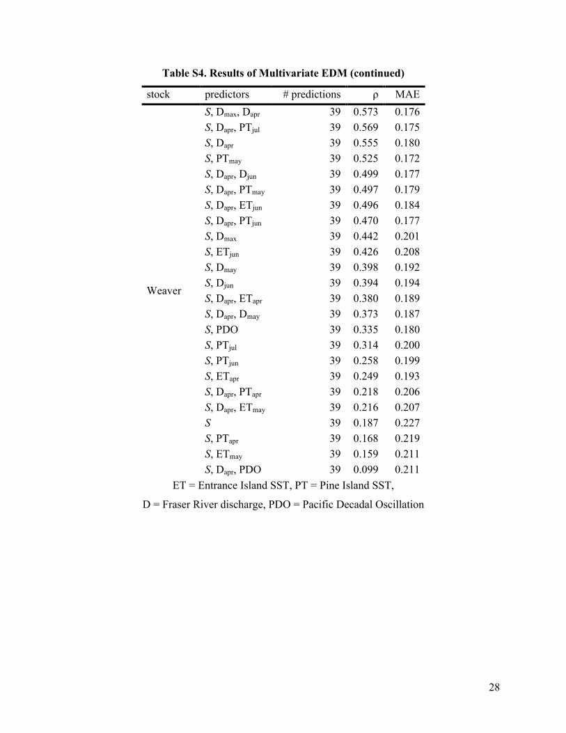
Table S4. Results of Multivariate EDM (continued)
stock predictors # predictions ρ MAE
Weaver
S, Dmax, Dapr 39 0.573 0.176 S, Dapr, PTjul 39 0.569 0.175 S, Dapr 39 0.555 0.180 S, PTmay 39 0.525 0.172 S, Dapr, Djun 39 0.499 0.177 S, Dapr, PTmay 39 0.497 0.179 S, Dapr, ETjun 39 0.496 0.184 S, Dapr, PTjun 39 0.470 0.177 S, Dmax 39 0.442 0.201 S, ETjun 39 0.426 0.208 S, Dmay 39 0.398 0.192 S, Djun 39 0.394 0.194 S, Dapr, ETapr 39 0.380 0.189 S, Dapr, Dmay 39 0.373 0.187 S, PDO 39 0.335 0.180 S, PTjul 39 0.314 0.200 S, PTjun 39 0.258 0.199 S, ETapr 39 0.249 0.193 S, Dapr, PTapr 39 0.218 0.206 S, Dapr, ETmay 39 0.216 0.207 S 39 0.187 0.227 S, PTapr 39 0.168 0.219 S, ETmay 39 0.159 0.211 S, Dapr, PDO 39 0.099 0.211
ET = Entrance Island SST, PT = Pine Island SST,
D = Fraser River discharge, PDO = Pacific Decadal Oscillation