Embed Size (px)
Citation preview

Support Vector Machines 支持向量机

Supervised learning Supervised learning
– An agent or machine is given N sensory inputs D = {x1, x2 . . . , xN}, as well as the desired outputs y1, y2, . . . yN, its goal is to learn to produce the correct output given a new input.
– Given D what can we say about xN+1?
Classification: y1, y2, . . . yN are discrete class labels, learn a labeling
function – Naïve bayes – Decision tree – K nearest neighbor – Least squares classification
( )f yx
2

Classification
Classification = learning from labeled data. Dominant problem in
Machine Learning
+
3

Linear Classifiers
4
Binary classification can be viewed as the task of separating classes in feature space(特征空间):
wTx + b = 0
wTx + b < 0 wTx + b > 0
h(x) = sign(wTx + b)
Decide if wTx + b > 0, otherwise

Linear Classification Which of the linear separators is optimal?
5

Classification Margin(间距)
• Geometry of linear classification • Discriminant function
• Important: the distance does not change if we scale
6

Classification Margin(间距) Distance from example xi to the separator is
Define the margin of a linear classifier as the width that the boundary could be increased by before hitting a data point
Examples closest to the hyperplane(超平面) are support vectors (支持向量). Margin m of the separator is the distance between support vectors.
wxw || br i
T +=
r
m
7

Maximum Margin Classification 最大间距分类
Maximizing the margin is good according to intuition and PAC theory.
Implies that only support vectors matter; other training examples are ignorable.
8

Maximum Margin Classification 最大间距分类
Maximizing the margin is good according to intuition and PAC theory.
Implies that only support vectors matter; other training examples are ignorable.
m
9
How do we compute m in term of w and b?

Maximum Margin Classification Mathematically
Let training set {(xi, yi)}i=1..N, xi∈Rd, yi ∈ {-1, 1} be separated by a hyperplane with margin m. Then for each training example (xi, yi):
For every support vector xs the above inequality is an equality. ys(wTxs + b) = c In the equality, we obtain that distance between each xs and the hyperplane is
wTxi + b ≤ - c if yi = -1 wTxi + b ≥ c if yi = 1
wwxw
wxw cbbr s
Tss
T
=+
=+
=)(y||
yi(wTxi + b) ≥ c ⇔
r
m
10

Maximum Margin Classification Mathematically
Then the margin can be expressed through w and b: Here is our Maximum Margin Classification problem: Note that the magnitude(大小) of c merely scales w and b, and does not
change the classification boundary at all! So we have a cleaner problem: This leads to the famous Support Vector Machines 支持向量机 — believed by
many to be the best "off-the-shelf" supervised learning algorithm
11

Learning as Optimization
12
Objective Function
Optimization Algorithm
Parameter Learning

Support Vector Machine • A convex quadratic programming(凸二次规划) problem with linear constraints:
– The attained margin is now given by – Only a few of the classification constraints are relevant support vectors
• Constrained optimization(约束优化)
– We can directly solve this using commercial quadratic programming (QP) code
– But we want to take a more careful investigation of Lagrange duality(对偶性), and the solution of the above in its dual form.
– deeper insight: support vectors, kernels(核) …
+ +
+
13

Quadratic Programming
Minimize (with respect to x) Subject to one or more constraints of the form: If , then g(x) is a convex function(凸函数): In this case
the quadratic program has a global minimizer Quadratic program of support vector machine:
0 Q
14

Solving Maximum Margin Classifier
Our optimization problem:
The Lagrangian:
Consider each constraint:
15

Solving Maximum Margin Classifier
Our optimization problem:
The Lagrangian:
Lemma:
(1) can be reformulated as The dual problem(对偶问题): 16

The Dual Problem(对偶问题) We minimize L with respect to w and b first:
Note that the bias term b dropped out but had produced a
“global” constraint on
Note: d(Ax+b)T(Ax+b) = (2(Ax+b)TA) dx d(xTa) = d(aTx) = aT dx
17

The Dual Problem(对偶问题)
We minimize L with respect to w and b first:
Note that (2) implies
Plug (4) back to L, and using (3), we have
18

The Dual Problem(对偶问题) Now we have the following dual optimization problem: This is a quadratic programming problem again
– A global maximum can always be found But what’s the big deal?
1. w can be recovered by 2. b can be recovered by 3. The “kernel”—核 more later…
19

Support Vectors
If a point xi satisfies
Due to the fact that
We have w is decided by the points with non-zero α’s
20

Support Vectors
only a few αi's can be nonzero!!
21

Support Vector Machines
Once we have the Lagrange multipliers αi, we can reconstruct the parameter vector w as a weighted combination of the training examples:
For testing with a new data x’ Compute and classify x’ as class 1 if the sum is positive, and class 2
otherwise Note: w need not be formed explicitly
22

Interpretation(解释) of support vector machines
• The optimal w is a linear combination of a small number of data points. This “sparse稀疏” representation can be viewed as data compression(数据压缩) as in the construction of kNN classifier
• To compute the weights αi, and to use support vector machines we need to specify only the inner products内积 (or kernel) between the examples
• We make decisions by comparing each new example x’ with only the support vectors:
23

Soft Margin Classification
What if the training set is not linearly separable? Slack variables(松弛变量) ξi can be added to allow
misclassification of difficult or noisy examples, resulting margin called soft.
ξi
ξi
24

Soft Margin Classification Mathematically
“Hard” margin QP: Soft margin QP: Note that ξi=0 if there is no error for xi ξi is an upper bound of the number of errors Parameter C can be viewed as a way to control “softness”: it
“trades off(折衷,权衡)” the relative importance of maximizing the margin and fitting the training data (minimizing the error). – Larger C more reluctant to make mistakes
25

The Optimization Problem
The dual of this new constrained optimization problem is
This is very similar to the optimization problem in the linear separable case, except that there is an upper bound C on αi now
Once again, a QP solver can be used to find αi
27

Roadmap
28
SVM Prediction
Loss Minimization
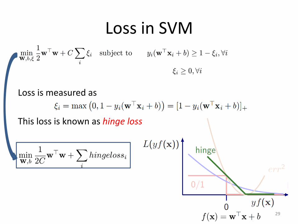
Loss in SVM
Loss is measured as
This loss is known as hinge loss
29

Loss functions
• Regression – Squared loss L2 – Absolute loss L1
• Binary classification
– Zero/one loss L0/1 (no good algorithm) – Squared loss L2 – Absolute loss L1 – Hinge loss (Support vector machines) – Logistic loss (Logistic regression)
31

Linear SVMs: Overview The classifier is a separating hyperplane.
Most “important” training points are support vectors; they define the
hyperplane.
Quadratic optimization algorithms can identify which training points xi are support vectors with non-zero Lagrangian multipliers αi.
Both in the dual formulation of the problem and in the solution training points appear only inside inner products: Find α1…αN such that Q(α) =Σαi - ½ΣΣαiαjyiyjxi
Txj is maximized and (1) Σαiyi = 0 (2) 0 ≤ αi ≤ C for all αi
f(x) = ΣαiyixiTx + b
32

Non-linearity: example
• Input x: – Patient information and vital signs
• Output y: – Health (positive is good)
33

Features in linear space
• Philosophy: extract any features that might be relevant.
• Features for medical diagnosis: height, weight, body temperature, blood pressure, etc.
• Three problems: non-monotonicity, non-linearity, interactions between features
34

Non-monotonicity
• Features: φ(x) = (1; temperature(x))
• Output: health y
• Problem: favor extremes; true relationship is non-monotonic
35

Non-monotonicity
• Solution: transform inputs
• φ(x) = (1; (temperature(x)-37)2)
• Disadvantage: requires manually-specied domain knowledge
36

Non-monotonicity
• φ(x) = (1; temperature(x); temperature(x)2)
• General: features should be simple building blocks to be pieced together
37

Interaction between features
• φ(x) = (height(x); weight(x))
• Output: health y
• Problem: can't capture relationship between height and weight
38

Interaction between features
• φ(x) = (height(x)-weight(x))2
• Solution: define features that combine inputs
• Disadvantage: requires manually-specified
domain knowledge
39

Interaction between features
• φ(x)=[height(x)2;weight(x)2; height(x)weight(x)] cross term
• Solution: add features involving multiple
measurements
40

Linear in what?
Prediction driven by score: w · φ(x) – Linear in w? Yes – Linear in φ(x)? Yes – Linear in x? No!
Key idea: non-linearity
– Predictors fw(x) can be expressive non-linear functions and decision boundaries of x.
– Score w · φ(x) is linear function of w and φ(x)
41

Non-linear SVMs Datasets that are linearly separable with some noise work out great:
But what are we going to do if the dataset is just too hard?
How about… mapping data to a higher-dimensional space:
0
0
0
x2
x
x
x
42
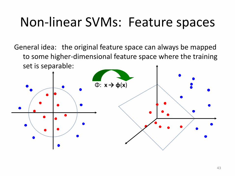
Non-linear SVMs: Feature spaces
General idea: the original feature space can always be mapped to some higher-dimensional feature space where the training set is separable:
Φ: x → φ(x)
43

The “Kernel Trick” Recall the SVM optimization problem
The data points only appear as inner product • As long as we can calculate the inner product in the feature
space, we do not need the mapping explicitly • Many common geometric operations (angles, distances) can
be expressed by inner products Define the kernel function K by K(xi,xj)= φ(xi)
T φ(xj)
44

Kernel methods
• Features viewpoint: construct and work with φ(x) (think in terms of properties of inputs)
• Kernel viewpoint: construct and work with K(xi,xj) (think in terms of similarity between inputs)
45

An Example for feature mapping and kernels
46

More Examples of Kernel Functions • Linear: K(xi,xj)= xi
Txj – Mapping Φ: x → φ(x), where φ(x) is x itself
• Polynomial(多项式) of power p: K(xi,xj)= (1+ xi
Txj)p
• Gaussian (radial-basis function径向基函数): K(xi,xj) = – Mapping Φ: x → φ(x), where φ(x) is infinite-dimensional
• Higher-dimensional space still has intrinsic dimensionality d,
but linear separators in it correspond to non-linear separators in original space.
2
2 i j
e σ
−−
x x
47

Kernel matrix
Suppose for now that K is indeed a valid kernel corresponding to some feature mapping φ, then for x1, …, xn, we can compute an n×n matrix {Ki,j} where Ki,j = φ(xi)
Tφ(xj) This is called a kernel matrix! Now, if a kernel function is indeed a valid kernel, and its
elements are dot-product in the transformed feature space, it must satisfy: – Symmetry K=KT
– Positive-semidefinite(半正定)
48

Matrix formulation
49

Nonlinear SVMs – RBF Kernel
50

Summary: Support Vector Machines
Linearly separable case Hard margin SVM – Primal quadratic programming – Dual quadratic programming
Not linearly separable? Soft margin SVM Non-linear SVMs
– Kernel trick
51

Summary: Support Vector Machines
SVM training: build a kernel matrix K using training data – Linear: K(xi,xj)= xi
Txj
– Gaussian (radial-basis function径向基函数): K(xi,xj) =
solve the following quadratic program SVM testing: now with αi, recover b,
we can predict new data points by:
2
2
σ
ji
exx −
−
52

作业
• 已知正例点 , 负例点 ,试求Hard Margin
SVM的最大间隔分离超平面和分类决策函数,
并在图上画出分离超平面、间隔边界及支持向量。
53
ΤΤΤ === )3,3(,)3,2(,)2,1( 321 xxxΤΤ == )2,3(,)1,2( 54 xx