Support Vector Machines for Analog Circuit PerformanceRepresentation

F. De Bernardinis†§

fdb@eecs.berkeley.edu

M. I. Jordan†

jordan@cs.berkeley.edu

A.SangiovanniVincentelli†

alberto@eecs.berkeley.edu†Department of Electrical Engineering §Dipartimento di Ingegneria

and Computer Science dell’InformazioneUniversity of California, Berkeley Universita di Pisa, Italy

ABSTRACTThe use of Support Vector Machines (SVMs) to representthe performance space of analog circuits is explored. In ab-stract terms, an analog circuit maps a set of input designparameters to a set of performance figures. This functionis usually evaluated through simulations and its range de-fines the feasible performance space of the circuit. In thispaper, we directly model performance spaces as mathemati-cal relations. We study approximation approaches based ontwo-class and one-class SVMs, the latter providing a bettertradeoff between accuracy and complexity avoiding “curseof dimensionality” issues with 2-class SVMs. We proposetwo improvements of the basic one-class SVM performances:conformal mapping and active learning. Finally we developan efficient algorithm to compute projections, so that top-down methodologies can be easily supported.

Categories and Subject DescriptorsB.7.2 [Integrated Circuits]: Design Aids-Verification

General TermsAlgorithms

1. INTRODUCTIONAnalog design has been traditionally a difficult discipline

of IC design. While in digital designs functionality dependson discrete sequences of discrete (binary) signals, continu-ous sequences (waveforms) of continuous values encode theinformation we need to manipulate and use in the analogcase. For this reason, any second-order physical effect mayhave a significant impact on function and performance ofan analog circuit. The effect of the choice of design param-eters such as transistor size and layout on performance isusually computed by simulation. Since simulations requirecompletely specified circuits to compute performances, thecomplexity of setting up simulations for system level explo-

Permission to make digital or hard copies of all or part of this work forpersonal or classroom use is granted without fee provided that copies arenot made or distributed for profit or commercial advantage and that copiesbear this notice and the full citation on the first page. To copy otherwise, torepublish, to post on servers or to redistribute to lists, requires prior specificpermission and/or a fee.DAC 2003,June 2–6, 2003, Anaheim, California, USA.Copyright 2003 ACM 1-58113-688-9/03/0006 ...$5.00.

ration is daunting even if we do not consider its computa-tional cost and the size of the search space. For this rea-son, behavioral models are currently used at the first stagesof designs to partition heuristically system constraints onindividual blocks. However, this is carried out in a purefunctional way, without any notion of the underlying feasi-ble performance space and tradeoffs. Building an approx-imate representation of the performance space is of greatinterest for providing behavioral models with architecturalconstraints that can fully enable top-down design method-ologies [1]. In the 70s and early 80s, a number of approaches[2] have been proposed to approximate the relation betweencircuit performance and parameters in explicit form. In par-ticular, the design problem tackled was to identify the valueof the design parameters that would yield a point in the per-formance space meeting a set of requirements expressed asinequalities. Assuming that the region of points satisfyingthe requirements is convex, the boundaries of the region wereapproximated by a set of hyperplanes (simplicial approxima-tion [3]) or by quadratic functions. If the exploration of thefeasible region was part of an optimization procedure, thesimplicial or quadratic approximation was refined locally toobtain a smaller error and yield an optimization procedurethat would eventually converge to an optimal point.

In this paper, we take a slightly different view of the prob-lem by directly modeling performances themselves in placeof parameter-performance relations. We improve upon theexisting techniques by exploiting recent results on learningand approximation techniques. In particular, we want todirectly represent the feasibility of achieving particular per-formances for a given topology of a circuit. This can beviewed as the problem of estimating the support of a set,and treated statistically as a quantile estimation problem.

2. BACKGROUNDSystem level analog design is a process largely dominated

by heuristics. Given a set of specifications/requirementsthat describe the system to be realized, the selection of anoptimal implementation architecture comes mainly out ofexperience. Usually, what is achieved is just a feasible pointat the system level, while optimality is sought locally atthe circuit level. The reason for this is the difficulty in theanalog world of knowing if something is realizable withoutactually attempting to design the circuit. The number of ef-fects to consider and their complex interrelations make thisproblem approachable only through the experience comingfrom past designs. System level optimization is extremely

hard because of the difficulties that hierchical designs face inabstracting single block behaviors and establishing cost andfeasibility without further knowledge of the implementationarchitecture and topology.

To cope with these problems, the Analog Platform con-cept has been proposed in [4] extending the one developedfor the digital world. The term Analog Platform (AP) indi-cates an architectural resource to map analog functionalitiesduring early system level exploration phases and constrainexploration to the feasible space of the considered imple-mentation (or set of implementations). Therefore, an APconsists of a set of behavioral models and of matching perfor-mance models. Behavioral models are parameterized mathe-matical models of the analog functionality that introduce atthe functional level a number of non-idealities attributableto the implementation and not intrinsic in the functionalityitself, such as distortion, bandwidth limitations, and noise.Non-ideal effects, as well as the principal performance fig-ures of the functionality (e.g. gain, power consumption andarea) are embedded in the behavioral models in the form ofparameters. Performance models constrain these parame-ters to satisfy a mathematical relation so that only feasibleinstances of the behavioral model (models with a completeset of parameter values) can be selected with respect of theconsidered architecture. In this paper we provide the detailsof the performance representation mechanism presented in[4], showing how they can be derived from sample data.

Other methods for building analog models from simula-tion data are mostly based on regression mechanisms. Agiven performance figure is fit on a set of regressors that arefunction of physical parameters of the circuit. An interest-ing model based on boosting methods has been recently pro-posed [5]. However, regression approaches are not suited totop-down methodologies where abstraction levels introduceopaqueness in the system hierarchy that hides the imple-mentation details needed for regression. Furthermore, eachperformance figure is fitted independently from the others,so that errors in capturing relations among different feasibleperformances may cumulate. An approach to model the fea-sible space has been proposed in [6]. In this paper we presenta novel approach to directly model performances that allowscapturing high dimensional performance spaces with effi-cient representations and provides the necessary means tosupport the multiple levels of abstraction required in top-down flows. Furthermore, it does not require that designersgenerate explicit models for their circuits, nor it asks them tocast their problems into specific mathematical frameworks.

3. PROBLEM FORMULATIONTop-down flows incrementally process designs through a

sequence of abstraction levels until final implementation isachieved. At each level of abstraction top-down methodolo-gies only deal with parameters present at the current levelto transform a given set of requirements into next-level con-straints. For example, if we are exploring the use of anamplifier at a given point in a design, our main interest isin selecting the optimal amplifier instance with respect to agiven set of performance figures, such as gain, power, noise,etc. Looking at the next (more detailed) level of abstraction,gain, power and noise can be placed in effect/cause relationwith a given amplifier topology, bias point and device siz-ing, which should not be considered at the current level ofabstraction. This implies that classic regression schemes for

Ld

Ibias

LsLs

Lg LgM2M1

M3 M4

Vbias

VoutLd

Figure 1: Schematic of the LNA modeled in this paper.Throughout the modeling process, the input impedance ismatched to 50Ω and the differential pair is assumed with 2%maximum mismatch.

representing analog circuit performances are not the mostsuitable means of performance representation in top-downflows. Therefore, we propose modeling the performancesthemselves as mathematical relations on performance fig-ures (effects), discarding the information on the relative pa-rameters (causes) as not pertinent at the current level ofabstraction. To approach the problem quantitatively, weintroduce the following definitions:

1. Input space I - Given a circuit C and m parameterscontrolling its instances, IC ⊆ Rm is the set of m-tuples(parameter values) over which we want to characterizeC.

2. Output space O - Given a circuit C and n performancefigures completely characterizing its behavioral model,OC ⊆ Rn is the set of m-tuples (performance values)that are achievable by C.

3. Evaluation function φ - Given a circuit C, IC and OC,φC : I → O allows translating a parameter m-tupleset into a performance n-tuple set.

4. Performance relation P - Given a circuit C, IC, OCand φC, we define the performance relation of C givenIC and φC to be PC on Rn that hold only for pointso ∈ OC. With a little abuse in notation, we will denoteboth the performance relation characteristic functionχP(x) : Rn → 0, 1 and the relation itself with PC(x).

Unfortunately, very little is known a priori about φC; cir-cuits are nonlinear systems so complex that it is difficult toderive any strong property concerning OC or PC. However,it is usually the case that the control set IC of interest is aregion of Rm where φC can be assumed to be continuous. Ifwe also assume I to be a connected set (or a union of con-nected sets), then O will be a (union of) connected set aswell, which is the only property we will exploit for buildingthe approximation of PC.

Even when the continuity assumption does not strictlyhold in I, the set of performances that we are interestedin modeling usually relates to circuits with well determinedoperating characteristics (performance invariant µ(x) = 1).For example, when we look at an oscillator we are not con-cerned in modeling points where it does not oscillate andthat would introduce an abrupt discontinuity in its perfor-mance figures. As long as the circuit remains in that op-erating mode, we can assume its performance to vary with

continuity when we span I. Therefore, we are actually in-terested in an effective I∗ = φ−1(x ∈ O s.t. µ(x) = 1),which makes the continuity assumption true.

In this paper we use the Low Noise Amplifier (LNA) forwireless applications shown in Figure 1 as a case study. Forsimplicity, ILNA has been taken as a hypercube in R7, and alarge number of simulations randomly spanning this hyper-cube were run to collect data for the experiments. ILNA

includes the sizes of M1-M2 and M3-M4 (2% maximummismatch), the bias current, the output load and the cur-rent mirror size. OLNA also lies in R7 and includes gain,noise, power, second and third order harmonic distortion,bandwidth and ripple in frequency response. Therefore,φLNA : R7 → R7 and PLNA : R7 → 0, 1.

4. SUPPORT VECTOR MACHINESSupport Vector Machines were first proposed in 1992 [7]

to solve machine learning problems. Machine learning con-sists in classifying points in a large input space as satisfyinga potentially complex unknown relation given a set of ex-periments that answer the question for a training set in theinput space. The training set populates the “performance”function space with points that are either satisfying or notthe relation. The task is to approximate the performancefunction based on the knowledge of the training set, so thata point in the input space not part of the training set could becorrectly classified. A general principle to select an approx-imant that is consistent with the training set and has goodproperties in classifying inputs, is the so called Occam’s ra-zor that can be used to set up an appropriate optimizationproblem.

A most important characteristic of an approximation sche-me is the choice of the basis functions, i.e., of those buildingblocks that can be chosen to optimize the likelihood of beingcorrect on the inputs not in the training set. We proposeSupport Vector Machines (SVMs) as a way of approximatingthe performance relation P. These approximating functionsare of the form

f(x) = sign(∑

i

αie−γ|x−xi|2 − ρ) (1)

where xi are input samples, αis are weighting multipliers,ρ is a constant, γ is a parameter controlling the fit of theapproximation and the sum is over a proper set of samples(support vector set).

SVMs belong to the class of hyper-plane classifiers thatseparate data points according to which side of a hyper-plane they fall. Non-linear mappings ψ(·) of the input sam-ples into a high dimensional feature space are exploited so toincrease data separability through hyperplanes. More specif-ically, SVMs exploit mapping to Hilbert spaces through ker-nel functions, so that a kernel k(x, ·) is associated at eachpoint x. In this paper, because of the weak properties thatwe have on P, the Gaussian (Radial Basis Function - RBF)kernel is chosen,

k(x, x′) = e−γ·‖x−x′‖2 (2)

where γ is a parameter of the kernel and controls the “width”of the kernel function around x. In paragraph 5.3 we show amethod to modify the kernel function to improve the approx-imation accuracy. The optimal hyperplane is representedby a small fraction of the original training data and can be

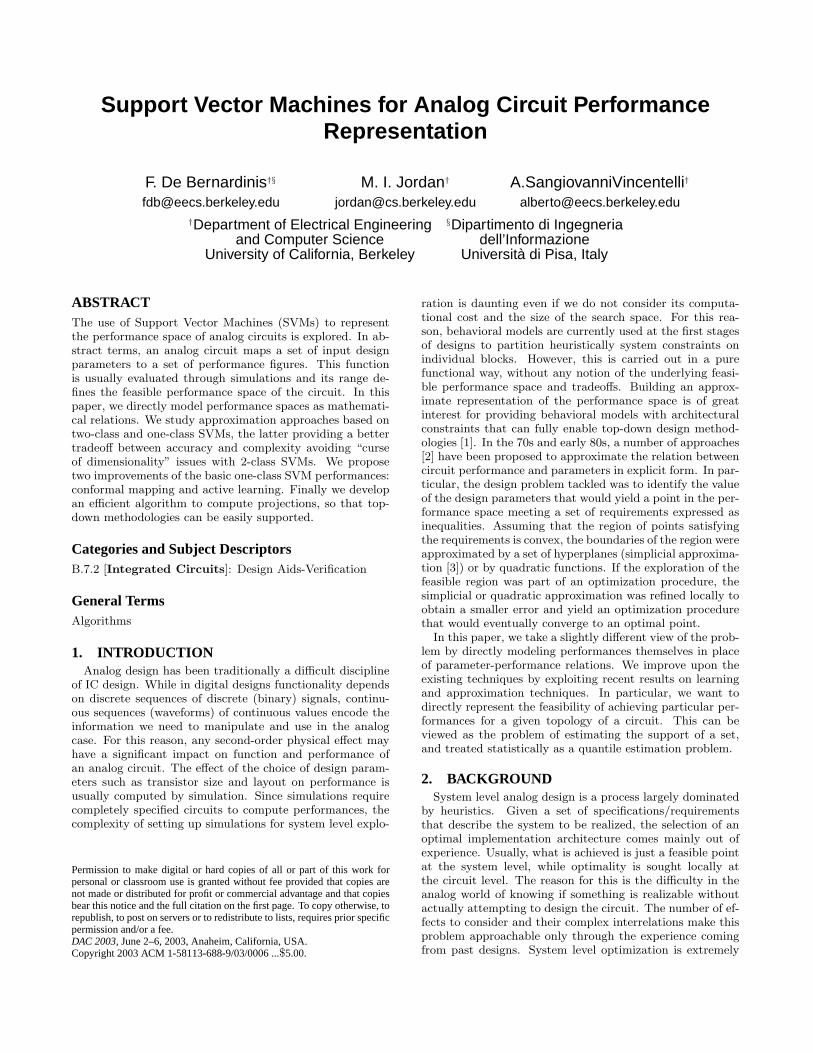
Figure 2: Plots of HD3 vs HD2 used as a reference patternfor the visual inspection for false positives. The projections havebeen obtained from 4-dimensional SVMs trained using mixturesof pcompl(·) and pWN (·) to generate −1 samples.

computed very efficiently through the following optimizationproblem:

minw,ξ,ρ,b

1

2‖w‖2 +

1

m

∑i

ξi − νρ (3)

s.t. yi(w · xi + b) ≥ ρ− ξi, ρ, ξi ≥ 0

where xi = ψ(xi) are the training samples, yi are the train-

ing labels, m is the number of samples, w =∑nSV

i=1 yiαixi

defines the optimal hyperplane in terms of a linear combina-tion of samples and nSV is the number of support vectors.The parameter ν provides an intuitively appealing control onsome of properties of the SVM; most importantly ν providesan upper bound on the fraction of false negatives (outliers).

In Section 5.1 we rely on a standard two-class SVM clas-sifiers to build an approximation for P. A more direct ap-proach, however, is to make use of the so-called “one-classSVM” [8]. Since the characteristic functions of the perfor-mance relations being considered are deterministic, the sup-port regions show sharp boundaries. The SVM approachalso holds open the promise of obtaining representations ofthe performance space at varying levels of abstraction, pro-viding needed flexibility for the design process. In Section 6,we investigate an approach for achieving such abstractionthat makes use of the computational properties of the SVMapproach.

5. SVM APPROXIMATIONS OF PThe accuracy of an approximation P is ideally assessed

by two quantities: the rate of false negatives and the rateof false positives. In our problem, false positives representa more serious problem than false negatives. In fact, top-down methodologies rely on predicted performances beingachievable when partitioning constraints over all the blocksin the system; therefore, a false positive would make theresulting design not feasible. On the other hand, false nega-tives may prevent us to achieve a better point but the designwould still be feasible. Although false positives are of greatinterest, they are also problematic to measure—since we usesimulation to generate samples, there is no constructive wayof generating points in Rn \ O.

In the attempt of gaining some initial insight into the rateof occurrence of false positives, we generated plots of some

Number of -1 #SV %Train %Test FP with 40krandom samples noise samples

20,000 2,164 98.76 93.55 74830,000 2,626 97.08 92.07 52240,000 3,056 93.70 90.11 335

Table 1: Performance of two-class (γ = 20, ν = 0.05, 5,000+1 samples). Large negative sets decrease the number of falsepositives, but for sets larger than 30,000 samples the false negativerates become significantly worse.

characteristic 2-D and 3-D projections of PLNA(·). Examplesof such plots are reported in Figure 2, where we show theprojection on a plane representing second-order harmonicdistortion (HD2) and third-order (HD3) for four differentestimators to be described in the following section. Esti-mators that place the estimated boundary around regionsthat contain few data points are oversmoothed, and pro-vide visual evidence of the need to choose smaller values ofregularization parameters.

We have also explored a more quantitative approach, ba-sed on the following intuition. Since O generally lies in alow-dimensional manifold in the ambient Euclidean space, ifdata are sampled throughout Rn, the number of true posi-tives (nTP ) is expected to be small relative to the number offalse positives (nFP ). Also, for reasonable values of the SVMparameters (γ — controls the width of the kernel around theith support vector—, and ν — controls false positives), suchthat the performance space is approximated as a connectedset, it is reasonable to expect that nTP should be nearlyindependent of the SVM parameters. This suggests that wemay be able to partition the number of positives, nP (γ, ν),from samples in Rn as follows:

nP (γ, ν) = nTP + nFP (γ, ν). (4)

Thus, based on the rate of variation of nP (γ, ν) with γ and ν,we can obtain a more quantitative basis for setting optimalvalues for γ and ν and thereby controlling the problematicfalse positive rate.

5.1 Two-class SVMOne approach to finding an approximation of O is to at-

tempt to use the powerful tools of two-class SVMs to forma discriminant boundary that separates O from its com-plement. This requires generating artificial “negative-class”data from the complement, and given that we are unable togenerate data from the complement set algorithmically (thesimulator only generates “positive-class” data), we must de-velop heuristics for generating such data. We have stud-ied three different heuristics for specifying suitable densityfunctions p(x), (x ∈ [−1, 1]7) that can be used to generate“negative-class” data:

• pWN (x) = constant ;

• pdata(x) =∏

i pi(xi), where pi(xi) is the empirical

marginal density function of points in O on the ith

dimension;

• pcompl(x) =∏

i qi(xi), where qi(xi) = pmax−pi(xi)pmax∆xi−1

,

∆xi = range of variable xi, is a complementary densityfunction of pi(xi) (in the sense that argmaxpi(xi) ≡argminqi(xi)).

The first approach places negative points independently ofthe actual O so that the number of points near the bound-

y = 0.0075x + 0.0278

y = 6.2076x-2.0934

0.00%

5.00%

10.00%

15.00%

20.00%

25.00%

30.00%

35.00%

40.00%

45.00%

0 5 10 15 20 25 30 35 40 45 50

Random Positives Test Error

Figure 3: Test error rates (false negatives) and random positiverates achieved by a one-class SVM trained with 5,000 samples andν = 0.05 as a function of γ. False negative rates are computedpresenting the SVM with 10,000 fresh samples, while randompositives with 80,000 random samples.

ary of P tends to be too small unless a very large numberof samples is used. The second approach approximates theregion where O is located to reduce the number of samplesneeded but tends to blur the region. The third approachplaces most points out of O, but tends to make the twoclasses “too separable” and overestimates P. All the ap-proaches have been experimentally evaluated and mixtureshave been considered as well. The color gradients in Fig-ure 2 show the effects of different complement generationheuristics on the projection accuracy. The color scale showsthat increasing the percentage of pdata(·) noise decreases theeffect of the positive pattern. Even though the region con-tour seems acceptable, the margins of the prediction (colorshades in the picture) are not as sharp as in the case obtainedwith pconst(·). Analogous plots obtained with pcompl(·) (notincluded) show regions that are too smooth.

Unfortunately, there is an intrinsic problem with 2-classSVM when applied to high dimensional problems relatedto curse-of-dimensionality issues. Considering a reducedO ∈ R4 for the LNA, a ratio of 5,000/30,000 positive-to-negative points is needed to provide a reasonable tradeoffbetween FP and FN rates (cf. Table 1). Given that O is amanifold of low-dimension, we expect this imbalance to beexponentially worse for higher dimensionality of O. More-over, the imbalance in number of data skews the classifica-tion boundary in ways that are difficult to predict. In gen-eral, none of the heuristics for generating “negative-class”data provide intuitive, effective general parameters for con-trolling performance tradeoffs, and are subject to possiblylarge, ill-defined biases.

5.2 One-class SVMOne-class SVMs were originally introduced as a means of

estimating quantiles of a probability density function [8].One-class SVMs require samples from only one class of data(positive class) (assuming negative class elsewhere) and com-pute the optimal hyperplane maximizing the separation ofdata from the origin. As a consequence, even if minimumsupport estimation is attempted through the training pro-cess, there is no explicit penalty in having a large supportregions in O. In fact, all the bounds available for one-classSVM predictors concern the probability of false negatives,i.e. that a sample drawn from p(x) might be misclassifiedby the machine.

Training of one-class SVMs is achieved by solving a qua-dratic optimization problem whose structure is analogous to

that of two-class SVMs:

minw,ξ,ρ

1

2‖w‖2 +

1

νm

∑i

ξi − ρ (5)

s.t. w · xi ≥ ρ− ξi, ξi ≥ 0

As with two-class SVMs, there are efficient algorithms tosolve this quadratic programming problem that exploit struc-tural properties of SVMs, e.g. [9] [10]. We based our imple-mentation on libsvm [11], and we trained SVMs with up to50,000 samples in very reasonable time (10’s of minutes).

Differently from the two class formulation (3), there is noexplicit penalties for false positives in (5) — all yis are +1.As a consequence, larger values of γ in the RBF kernel are re-quired to achieve tight approximations for the performanceregion. In our case, for moderate values of γ (< 5 ≈ 8), thenumber of positives (eqn. 4) represents a major problem, ascan be seen from Figure 3. Increasing γ reduces the numberof positives. However, the performance in terms of general-ization becomes worse than in the two-class case, as reportedin Table 2 (false negatives are about 8% higher than com-parable two-class SVMs). Finally, SVMs tend to degenerateinto Parzer window estimators as larger and larger valuesfor γ are used.

5.3 Improving accuracyThe accuracy of the estimator can be improved by en-

hancing the resolution in the support region boundaries.Since the underlying problem is deterministic, the transitionacross the boundary should be sharp. One way to achieveimproved resolution is via conformal transformation. Thisapproach was described in the context of the two-class SVMby [12] and [13], but the basic idea is also applicable tothe one-class SVM. In particular, an initial estimate of theboundary is provided by prior training of an SVM. Since sup-port vectors are located on the boundary of the hyperplanein feature space, they provide information about the regionthat is to undergo expansion. This expansion is achieved viaa conformal transformation:

k(x, x′) = c(x) · k(x, x′) · c(x′). (6)

Possible conformal transformations include:

c1(x) =∑

i

αi · e−γ‖x−xi‖2 , c2(x) =∑

i

e−ζi‖x−xi‖2 (7)

where ζi = 1M

∑j ‖xη|j − xj‖2, and where xη|j is the jth

nearest neighbor of xi. αi and xi refer to an SVM previ-ously trained on the same dataset. Our results with bothconformal transformations show significant performance im-provements (see Table 2), with c1(x) performing slightlybetter than c2(x). However, the results achievable with ac-tive learning schemes (sec.5.4) and the complexity of pro-jections over transformed kernels (sec.6) make their use lessattractive.

5.4 Active learningBecause one-class SVMs estimate the degree of novelty of

a given vector, it is possible to exploit misclassified samplesas seeds for further sample generation, thus forcing the sam-pling scheme to place more points where fewer are present[2]. Ideally, all the training samples should be correctly clas-sified, but the need to regularize forces a fraction of thetraining samples to be misclassified (controlled via the pa-rameter ν). We can exploit such false negatives as follows.

−0.3

−0.25

−0.2

−0.15

−0.1

−0.05

0

0.05

5 10 15 20 25 30

5

10

15

20

25

30Number of samples: 1224

−0.25

−0.2

−0.15

−0.1

−0.05

0

0.05

5 10 15 20 25 30

5

10

15

20

25

30Number of samples: 1704

−0.25

−0.2

−0.15

−0.1

−0.05

0

0.05

5 10 15 20 25 30

5

10

15

20

25

30Number of samples: 2322

−0.25

−0.2

−0.15

−0.1

−0.05

0

0.05

5 10 15 20 25 30

5

10

15

20

25

30Number of samples: 3065

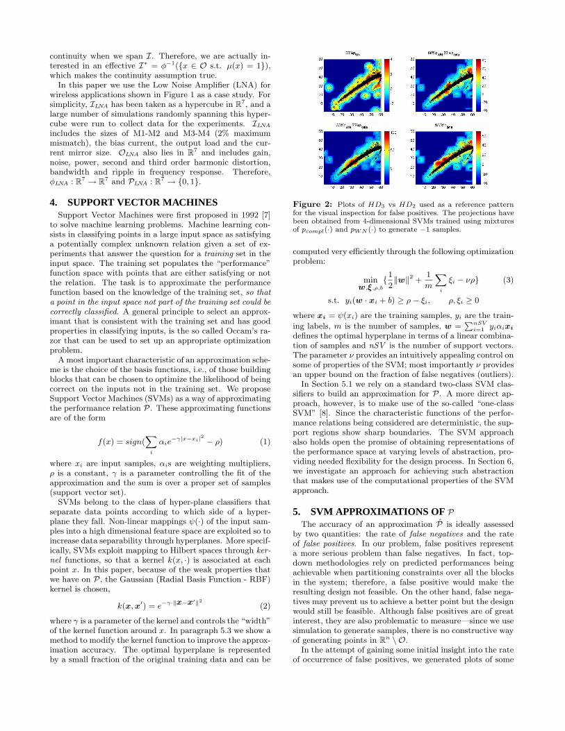
Figure 4: Results achieved interleaving training with gen-eration of new data samples. Starting from 1,000 pointsrandomly sampled, 4 iterations were completed with ν =0.1, 0.08, 0.06, 0.04 and γ = 10, 15, 20, 25. The final SVMemphasizes a complex pattern in the performance space that wasnot present in SVMs obtained from a larger number of randomsamples.

For each such false negative os, we can reinforce the informa-tion content of the data point (i.e. its novelty) by generatingnew samples on, in the neighborhood of os. One way toachieve this is by applying small random perturbations tothe input vector is. Even if the simulation function φC is notbijective, we can store the mapping it → ot to get is.The set in is then simulated to generate a new sample O′.A new SVM is then trained on O∪O′ and the process is iter-ated. As a consequence, the accuracy of the approximationP of P is increased.

We tested the approach by running five simulation/trainiterations, starting from a data set consisting of 1,000 sam-ples and selecting 5% more samples each time. We startedwith relatively small values of γ and relatively large valuesfor ν because these combinations of parameters produce verysmooth support regions that allow to better isolate “novel”points. In successive iterations, γ was increased while ν de-creased using a sort of annealing schedule leading to thefinal SVM reported in Figure 4. For each selected sample avariable number of new simulation points was generated de-pending on the value of the decision function (the more neg-

ative, the more simulations). The resulting PLNA,5 (trainedon 3,065 samples, Figure 4) yields excellent performance,displaying features that were not present in SVMs trainedwith uniformly sampled datasets containing 5,000 samples.

6. PROJECTIONS ONPGiven the nature of top-down flows, the same circuit may

be considered at different levels of abstraction in the designprocess. As a consequence, given an analog circuit C andits performance relation PC(x), x ∈ Rn, it is often the casethat at a high level of abstraction we are interested in a

lower-dimensional relation P ′C(x′) with x′ ∈ Rn′ , n′ < n.x′ is a projection of x that refers to a more abstract viewof the circuit. For example, x = [gain, bandwidth, noise,distortion], x′ = [gain, bandwidth]. The formal definition ofP ′(x′) is:

P ′(x′) =

1 if ∃x′′ s.t. P([x′x′′]) = 10 otherwise

Support Vector Machine %Train %Test O ν γ #SVTwo-Class pn(·) 97.08 92.07 R4 0.05 20 2,626Two-Class 0.66 pn(·) 0.33 pc(·) 95.66 93.06 R4 0.05 20 2,346Two-Class 0.66 pn(·) 0.33 pd(·) 71.12 60.58 R4 0.05 20 4,873Two-Class 0.6 pn(·) 0.2 pd(·) 0.2 pc(·). 97.84 91.81 R4 0.05 20 2,859One-Class 95.72 85.11 R4 0.05 20 764One-Class 95.20 79.67 R7 0.04 20 929One-Class prior c1(·) 96.15 84.57 R7 0.04 20 791One-Class prior c2(·) 95.97 84.39 R7 0.04 20 819

Table 2: Summary of SVM performance. The false negative rate on the training set is very good due to the ν-SVM formulation used,with the exception of the third row, which relies on pdata(·) to generate random samples (random samples blur the data pattern). Alltwo-class SVMs were trained with 30,000 random negative samples.

When working with SVMs, the problem becomes that offinding x′′ that makes the decision function positive givenx′. An equivalent condition is that the maximum of f(x) =∑

Sup.V ec. αik(x, xi)− ρ is positive, which generates a non-linear global optimization problem. However, the decisionfunction is a sum of Gaussian kernels that, in our case, havelarge γ parameters. Therefore, each point where such aGaussian is centered (i.e., each support vector) provides asmall neighborhood of a possible local optimum. Exploringthese points running a simple steepest ascent method fromthe support vectors, we can keep track of local optima andfind the global optimum more rapidly. We have implementedthis approach to compute projections. Some heuristics havealso been adopted to limit the number of support vectors tobe checked for optimality. If we rewrite the decision functionas:

f([x′x′′]) =∑

i

αie−γ‖x′−x′i‖2︸ ︷︷ ︸

αi

e−γ‖x′′−x′′i ‖2 , (8)

then if ‖x′−x′i‖ is “large” (x′ is fixed) αi will be very smalland so the support vector xi will not be a good candidate toget to the maximum. Furthermore, if the SVM had a globaloptimum in the neighbor of x′′i because of xi, then the SVMwould classify x based on a support vector whose compo-nents x′i are “far” from x′. This would be an inconsistentbehavior for an SVM based on RBF modeling O = φ(I)under the assumptions made in section 3. The condition‖x′ − x′i‖∞ > 0.1 provides a good heuristic for discard-ing support vectors. Given a candidate support vector xi

and the smoothness of the decision function, we found thata simple steepest ascent local optimizer suffices for findingthe optimum in fewer than 15 iterations. The complexity ofthe implemented algorithm is (n is the dimensionality of Pand l the number of support vectors) O(l2n) for the normalcase and O(l3n) for the conformal mapping case.

7. CONCLUSIONSWe presented a novel approach for modeling the perfor-

mance space of an analog circuit based on SVMs. The result-ing model provides a clear separation of abstraction levels,directly modeling performance relations in place of regres-sions on implementation parameters. An efficient projec-tion algorithm allows considering the same circuit at differ-ent levels of abstraction using the same underlying model.Therefore, the approach has preferred utilization in top-down design flows and analog platforms. SVMs are trainedon simulation data, and false positives are controlled basedon a randomized testing procedure. By augmenting the ba-sic one-class SVM to exploit conformal mappings and an

active learning methodology, we have obtained a satisfac-tory solution both in terms of accuracy and of reduction ofnumber of simulations required to model the circuit. Overallwe feel that one-class SVMs are quite promising as an ap-proach to finding representations of the performance spaceand as a component in an IC design system where top-downconstraint mapping is molded with bottom-up circuit blockcharacterizations.

8. REFERENCES

[1] A. Sangiovanni-Vincentelli, “Defining platform-based de-sign,” EE-Design, March 2002.

[2] R. Brayton and A. Hachtel, G.D.and Sangiovanni-Vincentelli, “A survey of optimization techniques forintegrated-circuit design,” Proceedings of the IEEE, vol. 69,pp. 1334–62, October 1981.

[3] S. Director, “The simplicial approximation approach to de-sign centering,” IEEE Transactions on Circuits and Sys-tems, vol. 24, pp. 363–72, July 1977.

[4] L. Carloni, F. De Bernardinis, A. Sangiovanni Vincentelli,and M. Sgroi, “The art and science of integrated systemsdesign,” in to be presented at ESSCIRC’02, September 2002.

[5] H. Liu, A. Singhee, R. Rutenbar, and L. R. Carley, “Re-membrance of circuits past: Macromodeling by data miningin large analog design spaces,” in Proceedings of DAC, 2002.

[6] R. Harjani and T. Tibshirani, “Feasibility and performanceregion modeling of analog and digital circuits,” in AnalogIntegrated Circtuis and Signal Processing, Kluwer AcademicPublishers, 1996.

[7] B. E. Boser, I. M. Guyon, and V. N. Vapnik, “A training al-gorithm for optimal margin classifiers,” in 5th Annual ACMWorkshop on COLT (D. Haussler, ed.), (Pittsburgh, PA),pp. 144–152, ACM Press, 1992.

[8] B. Scholkopf, J. Platt, J. Shawe-Taylor, A. J. Smola, andR. C. Williamson, “Estimating the support of a high-dimensional distribution,” Tech. Rep. MSR-TR-99-87, Mi-crosoft Research, 1999.

[9] J. Platt, “Sequential minimal optimization: A fast algorithmfor training support vector machines,” Tech. Rep. MSR-TR-98-14, Microsoft Research, 1998.

[10] T. Joachims, “Making large-scale svm learning practical,”in Advances in Kernel Methods - Support Vector Learning,MIT Press, 1998.

[11] C. Chang and C. Lin, “Training ν-support vector classifiers:Theory and algoritms,” Neural Computation, vol. 13, no. 9,pp. 2119–2147, 2001.

[12] S. Amari and S. Wu, “Improving support vector machineclassifiers by modifying kernel functions,” Neural Networks,no. 12, pp. 783–789, 1999.

[13] S. Amari and S. Wu, “Conformal transformation of kernelfunctions: A data-dependent way to improve support vec-tor machine classifiers,” Neural Processing Letters, no. 15,pp. 59–67, 2002.