Support Vector Machines

Here we approach the two-class classification problem in adirect way:

We try and find a plane that separates the classes infeature space.

If we cannot, we get creative in two ways:

• We soften what we mean by “separates”, and

• We enrich and enlarge the feature space so that separationis possible.

1 / 21

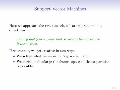
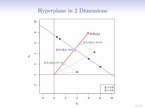
What is a Hyperplane?

• A hyperplane in p dimensions is a flat affine subspace ofdimension p− 1.

• In general the equation for a hyperplane has the form

β0 + β1X1 + β2X2 + . . .+ βpXp = 0

• In p = 2 dimensions a hyperplane is a line.

• If β0 = 0, the hyperplane goes through the origin,otherwise not.

• The vector β = (β1, β2, · · · , βp) is called the normal vector— it points in a direction orthogonal to the surface of ahyperplane.

2 / 21

Hyperplane in 2 Dimensions

−2 0 2 4 6 8 10

−2

02

46

810

X1

X2

●

●

●

●

●

β=(β1,β2)

β1X1+β2X2−6=0

β1X1+β2X2−6=1.6

●

β1X1+β2X2−6=−4

β1 = 0.8β2 = 0.6

3 / 21

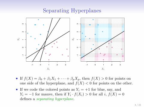
Separating Hyperplanes

−1 0 1 2 3

−1

01

23

−1 0 1 2 3

−1

01

23

X1X1

X2

X2

• If f(X) = β0 + β1X1 + · · ·+ βpXp, then f(X) > 0 for points onone side of the hyperplane, and f(X) < 0 for points on the other.

• If we code the colored points as Yi = +1 for blue, say, andYi = −1 for mauve, then if Yi · f(Xi) > 0 for all i, f(X) = 0defines a separating hyperplane.

4 / 21

Maximal Margin ClassifierAmong all separating hyperplanes, find the one that makes thebiggest gap or margin between the two classes.

−1 0 1 2 3

−1

01

23

X1

X2

Constrained optimization problem

maximizeβ0,β1,...,βp

M

subject to

p∑j=1

β2j = 1,

yi(β0 + β1xi1 + . . .+ βpxip) ≥Mfor all i = 1, . . . , N.

This can be rephrased as a convex quadratic program, andsolved efficiently. The function svm() in package e1071 solvesthis problem efficiently

5 / 21

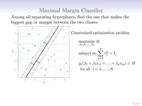
Maximal Margin ClassifierAmong all separating hyperplanes, find the one that makes thebiggest gap or margin between the two classes.

−1 0 1 2 3

−1

01

23

X1

X2

Constrained optimization problem

maximizeβ0,β1,...,βp

M

subject to

p∑j=1

β2j = 1,

yi(β0 + β1xi1 + . . .+ βpxip) ≥Mfor all i = 1, . . . , N.

This can be rephrased as a convex quadratic program, andsolved efficiently. The function svm() in package e1071 solvesthis problem efficiently

5 / 21

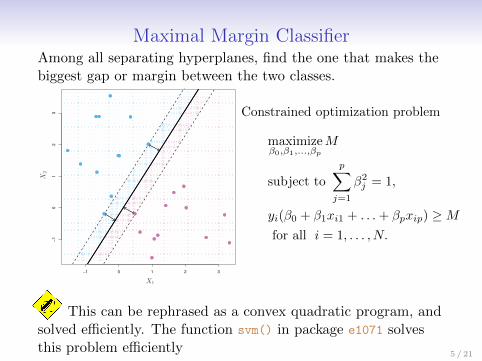
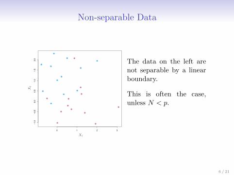
Non-separable Data

0 1 2 3

−1

.0−

0.5

0.0

0.5

1.0

1.5

2.0

X1

X2

The data on the left arenot separable by a linearboundary.

This is often the case,unless N < p.

6 / 21

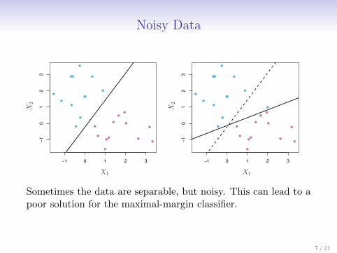
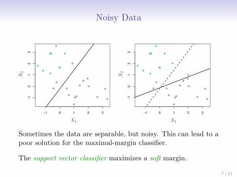
Noisy Data

−1 0 1 2 3

−1

01

23

−1 0 1 2 3

−1

01

23

X1X1X

2

X2

Sometimes the data are separable, but noisy. This can lead to apoor solution for the maximal-margin classifier.

The support vector classifier maximizes a soft margin.

7 / 21

Noisy Data

−1 0 1 2 3

−1

01

23

−1 0 1 2 3

−1

01

23

X1X1X

2

X2

Sometimes the data are separable, but noisy. This can lead to apoor solution for the maximal-margin classifier.

The support vector classifier maximizes a soft margin.

7 / 21

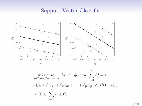
Support Vector Classifier

−0.5 0.0 0.5 1.0 1.5 2.0 2.5

−1

01

23

4

1

2

3

4 5

6

7

8

9

10

−0.5 0.0 0.5 1.0 1.5 2.0 2.5

−1

01

23

4

1

2

3

4 5

6

7

8

9

10

11

12

X1X1X

2

X2

maximizeβ0,β1,...,βp,ε1,...,εn

M subject to

p∑j=1

β2j = 1,

yi(β0 + β1xi1 + β2xi2 + . . .+ βpxip) ≥M(1− εi),

εi ≥ 0,

n∑i=1

εi ≤ C,

8 / 21

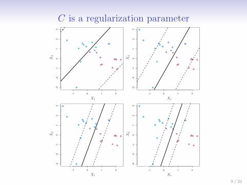
C is a regularization parameter

−1 0 1 2

−3

−2

−1

01

23

−1 0 1 2

−3

−2

−1

01

23

−1 0 1 2

−3

−2

−1

01

23

−1 0 1 2

−3

−2

−1

01

23

X1X1

X1X1

X2

X2

X2

X2

9 / 21

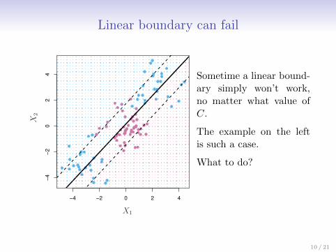
Linear boundary can fail

−4 −2 0 2 4

−4

−2

02

4

−4 −2 0 2 4

−4

−2

02

4

X1X1

X2

X2

Sometime a linear bound-ary simply won’t work,no matter what value ofC.

The example on the leftis such a case.

What to do?

10 / 21

Feature Expansion

• Enlarge the space of features by including transformations;e.g. X2

1 , X31 , X1X2, X1X

22 ,. . .. Hence go from a

p-dimensional space to a M > p dimensional space.

• Fit a support-vector classifier in the enlarged space.

• This results in non-linear decision boundaries in theoriginal space.

Example: Suppose we use (X1, X2, X21 , X

22 , X1X2) instead of

just (X1, X2). Then the decision boundary would be of the form

β0 + β1X1 + β2X2 + β3X21 + β4X

22 + β5X1X2 = 0

This leads to nonlinear decision boundaries in the original space(quadratic conic sections).

11 / 21

Feature Expansion

• Enlarge the space of features by including transformations;e.g. X2

1 , X31 , X1X2, X1X

22 ,. . .. Hence go from a

p-dimensional space to a M > p dimensional space.

• Fit a support-vector classifier in the enlarged space.

• This results in non-linear decision boundaries in theoriginal space.

Example: Suppose we use (X1, X2, X21 , X

22 , X1X2) instead of

just (X1, X2). Then the decision boundary would be of the form

β0 + β1X1 + β2X2 + β3X21 + β4X

22 + β5X1X2 = 0

This leads to nonlinear decision boundaries in the original space(quadratic conic sections).

11 / 21

Cubic PolynomialsHere we use a basisexpansion of cubic poly-nomials

From 2 variables to 9

The support-vector clas-sifier in the enlargedspace solves the problemin the lower-dimensionalspace

−4 −2 0 2 4

−4

−2

02

4

−4 −2 0 2 4

−4

−2

02

4

X1X1

X2

X2

β0+β1X1+β2X2+β3X21+β4X

22+β5X1X2+β6X

31+β7X

32+β8X1X

22+β9X

21X2 = 0

12 / 21

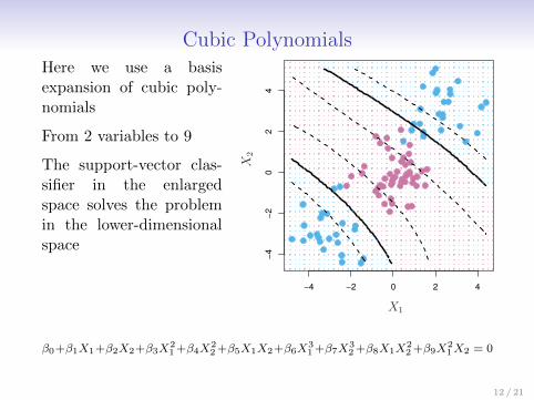
Cubic PolynomialsHere we use a basisexpansion of cubic poly-nomials

From 2 variables to 9

The support-vector clas-sifier in the enlargedspace solves the problemin the lower-dimensionalspace

−4 −2 0 2 4

−4

−2

02

4

−4 −2 0 2 4

−4

−2

02

4

X1X1

X2

X2

β0+β1X1+β2X2+β3X21+β4X

22+β5X1X2+β6X

31+β7X

32+β8X1X

22+β9X

21X2 = 0

12 / 21

Nonlinearities and Kernels

• Polynomials (especially high-dimensional ones) get wildrather fast.

• There is a more elegant and controlled way to introducenonlinearities in support-vector classifiers — through theuse of kernels.

• Before we discuss these, we must understand the role ofinner products in support-vector classifiers.

13 / 21

Inner products and support vectors

〈xi, xi′〉 =

p∑j=1

xijxi′j — inner product between vectors

• The linear support vector classifier can be represented as

f(x) = β0 +n∑i=1

αi〈x, xi〉 — n parameters

• To estimate the parameters α1, . . . , αn and β0, all we needare the

(n2

)inner products 〈xi, xi′〉 between all pairs of

training observations.

It turns out that most of the α̂i can be zero:

f(x) = β0 +∑i∈S

α̂i〈x, xi〉

S is the support set of indices i such that α̂i > 0. [see slide 8]

14 / 21

Inner products and support vectors

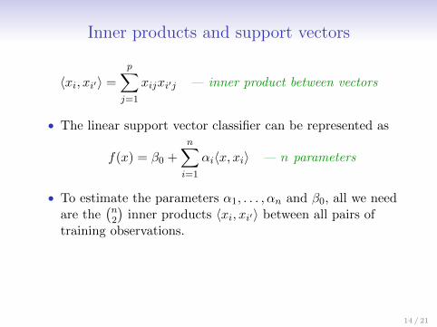
〈xi, xi′〉 =

p∑j=1

xijxi′j — inner product between vectors

• The linear support vector classifier can be represented as

f(x) = β0 +

n∑i=1

αi〈x, xi〉 — n parameters

• To estimate the parameters α1, . . . , αn and β0, all we needare the

(n2

)inner products 〈xi, xi′〉 between all pairs of

training observations.

It turns out that most of the α̂i can be zero:

f(x) = β0 +∑i∈S

α̂i〈x, xi〉

S is the support set of indices i such that α̂i > 0. [see slide 8]

14 / 21

Inner products and support vectors

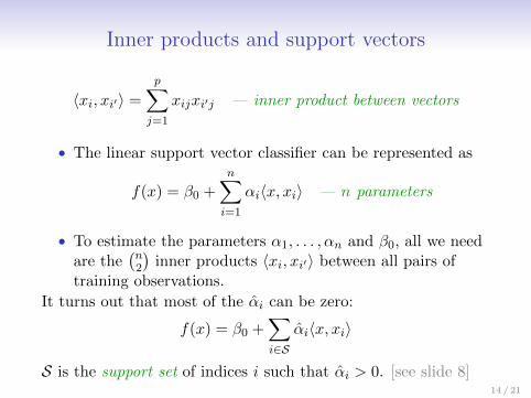
〈xi, xi′〉 =

p∑j=1

xijxi′j — inner product between vectors

• The linear support vector classifier can be represented as

f(x) = β0 +

n∑i=1

αi〈x, xi〉 — n parameters

• To estimate the parameters α1, . . . , αn and β0, all we needare the

(n2

)inner products 〈xi, xi′〉 between all pairs of

training observations.

It turns out that most of the α̂i can be zero:

f(x) = β0 +∑i∈S

α̂i〈x, xi〉

S is the support set of indices i such that α̂i > 0. [see slide 8]

14 / 21

Inner products and support vectors

〈xi, xi′〉 =

p∑j=1

xijxi′j — inner product between vectors

• The linear support vector classifier can be represented as

f(x) = β0 +

n∑i=1

αi〈x, xi〉 — n parameters

• To estimate the parameters α1, . . . , αn and β0, all we needare the

(n2

)inner products 〈xi, xi′〉 between all pairs of

training observations.

It turns out that most of the α̂i can be zero:

f(x) = β0 +∑i∈S

α̂i〈x, xi〉

S is the support set of indices i such that α̂i > 0. [see slide 8]14 / 21

Kernels and Support Vector Machines

• If we can compute inner-products between observations, wecan fit a SV classifier. Can be quite abstract!

• Some special kernel functions can do this for us. E.g.

K(xi, xi′) =

1 +

p∑j=1

xijxi′j

d

computes the inner-products needed for d dimensionalpolynomials —

(p+dd

)basis functions!

Try it for p = 2 and d = 2.

• The solution has the form

f(x) = β0 +∑i∈S

α̂iK(x, xi).

15 / 21

Kernels and Support Vector Machines

• If we can compute inner-products between observations, wecan fit a SV classifier. Can be quite abstract!

• Some special kernel functions can do this for us. E.g.

K(xi, xi′) =

1 +

p∑j=1

xijxi′j

d

computes the inner-products needed for d dimensionalpolynomials —

(p+dd

)basis functions!

Try it for p = 2 and d = 2.

• The solution has the form

f(x) = β0 +∑i∈S

α̂iK(x, xi).

15 / 21

Kernels and Support Vector Machines

• If we can compute inner-products between observations, wecan fit a SV classifier. Can be quite abstract!

• Some special kernel functions can do this for us. E.g.

K(xi, xi′) =

1 +

p∑j=1

xijxi′j

d

computes the inner-products needed for d dimensionalpolynomials —

(p+dd

)basis functions!

Try it for p = 2 and d = 2.

• The solution has the form

f(x) = β0 +∑i∈S

α̂iK(x, xi).

15 / 21

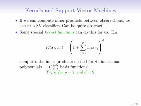
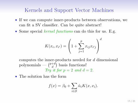
Kernels and Support Vector Machines

• If we can compute inner-products between observations, wecan fit a SV classifier. Can be quite abstract!

• Some special kernel functions can do this for us. E.g.

K(xi, xi′) =

1 +

p∑j=1

xijxi′j

d

computes the inner-products needed for d dimensionalpolynomials —

(p+dd

)basis functions!

Try it for p = 2 and d = 2.

• The solution has the form

f(x) = β0 +∑i∈S

α̂iK(x, xi).

15 / 21

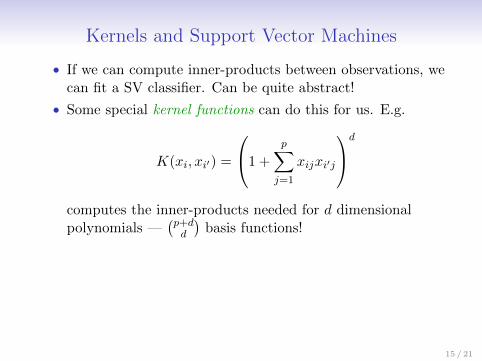
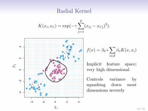
Radial Kernel

K(xi, xi′) = exp(−γp∑j=1

(xij − xi′j)2).

−4 −2 0 2 4

−4

−2

02

4

−4 −2 0 2 4

−4

−2

02

4

X1X1

X2

X2

f(x) = β0+∑i∈S

α̂iK(x, xi)

Implicit feature space;very high dimensional.

Controls variance bysquashing down mostdimensions severely

16 / 21

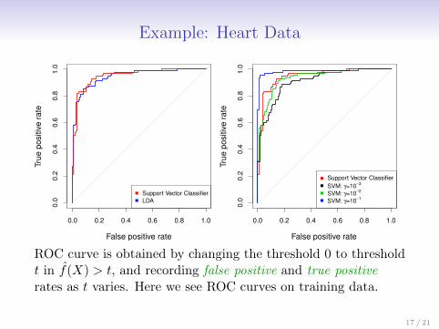
Example: Heart Data

False positive rate

Tru

e p

ositiv

e r

ate

0.0 0.2 0.4 0.6 0.8 1.0

0.0

0.2

0.4

0.6

0.8

1.0

Support Vector Classifier

LDA

False positive rate

Tru

e p

ositiv

e r

ate

0.0 0.2 0.4 0.6 0.8 1.0

0.0

0.2

0.4

0.6

0.8

1.0

Support Vector Classifier

SVM: γ=10−3

SVM: γ=10−2

SVM: γ=10−1

ROC curve is obtained by changing the threshold 0 to thresholdt in f̂(X) > t, and recording false positive and true positiverates as t varies. Here we see ROC curves on training data.

17 / 21

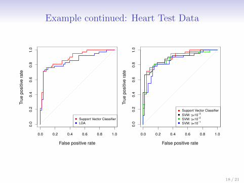
Example continued: Heart Test Data

False positive rate

Tru

e p

ositiv

e r

ate

0.0 0.2 0.4 0.6 0.8 1.0

0.0

0.2

0.4

0.6

0.8

1.0

Support Vector Classifier

LDA

False positive rate

Tru

e p

ositiv

e r

ate

0.0 0.2 0.4 0.6 0.8 1.00.0

0.2

0.4

0.6

0.8

1.0

Support Vector Classifier

SVM: γ=10−3

SVM: γ=10−2

SVM: γ=10−1

18 / 21

SVMs: more than 2 classes?

The SVM as defined works for K = 2 classes. What do we do ifwe have K > 2 classes?

OVA One versus All. Fit K different 2-class SVMclassifiers f̂k(x), k = 1, . . . ,K; each class versusthe rest. Classify x∗ to the class for which f̂k(x

∗)is largest.

OVO One versus One. Fit all(K2

)pairwise classifiers

f̂k`(x). Classify x∗ to the class that wins the mostpairwise competitions.

Which to choose? If K is not too large, use OVO.

19 / 21

SVMs: more than 2 classes?

The SVM as defined works for K = 2 classes. What do we do ifwe have K > 2 classes?

OVA One versus All. Fit K different 2-class SVMclassifiers f̂k(x), k = 1, . . . ,K; each class versusthe rest. Classify x∗ to the class for which f̂k(x

∗)is largest.

OVO One versus One. Fit all(K2

)pairwise classifiers

f̂k`(x). Classify x∗ to the class that wins the mostpairwise competitions.

Which to choose? If K is not too large, use OVO.

19 / 21

SVMs: more than 2 classes?

The SVM as defined works for K = 2 classes. What do we do ifwe have K > 2 classes?

OVA One versus All. Fit K different 2-class SVMclassifiers f̂k(x), k = 1, . . . ,K; each class versusthe rest. Classify x∗ to the class for which f̂k(x

∗)is largest.

OVO One versus One. Fit all(K2

)pairwise classifiers

f̂k`(x). Classify x∗ to the class that wins the mostpairwise competitions.

Which to choose? If K is not too large, use OVO.

19 / 21

SVMs: more than 2 classes?

The SVM as defined works for K = 2 classes. What do we do ifwe have K > 2 classes?

OVA One versus All. Fit K different 2-class SVMclassifiers f̂k(x), k = 1, . . . ,K; each class versusthe rest. Classify x∗ to the class for which f̂k(x

∗)is largest.

OVO One versus One. Fit all(K2

)pairwise classifiers

f̂k`(x). Classify x∗ to the class that wins the mostpairwise competitions.

Which to choose? If K is not too large, use OVO.

19 / 21

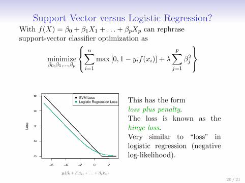
Support Vector versus Logistic Regression?With f(X) = β0 + β1X1 + . . .+ βpXp can rephrasesupport-vector classifier optimization as

minimizeβ0,β1,...,βp

n∑i=1

max [0, 1− yif(xi)] + λ

p∑j=1

β2j

−6 −4 −2 0 2

02

46

8

Lo

ss

SVM Loss

Logistic Regression Loss

yi(β0 + β1xi1 + . . . + βpxip)

This has the formloss plus penalty.The loss is known as thehinge loss.Very similar to “loss” inlogistic regression (negativelog-likelihood).

20 / 21

Which to use: SVM or Logistic Regression

• When classes are (nearly) separable, SVM does better thanLR. So does LDA.

• When not, LR (with ridge penalty) and SVM very similar.

• If you wish to estimate probabilities, LR is the choice.

• For nonlinear boundaries, kernel SVMs are popular. Canuse kernels with LR and LDA as well, but computationsare more expensive.

21 / 21