Support vector machines - ccs.neu.edu

101

Support vector machines

I’ve seen more than one book follow this pattern when discussing support vectormachines (SVMs): “Here’s a little theory. Now SVMs are too hard for you. Just down-load libsvm and use that.” I’m not going to follow that pattern. I think if you justread a little bit of the theory and then look at production C++ SVM code, you’regoing to have trouble understanding it. But if we strip out the production code andthe speed improvements, the code becomes manageable, perhaps understandable.

Support vector machines are considered by some people to be the best stock clas-sifier. By stock, I mean not modified. This means you can take the classifier in its basicform and run it on the data, and the results will have low error rates. Support vectormachines make good decisions for data points that are outside the training set.

In this chapter you’re going to learn what support vector machines are, and I’llintroduce some key terminology. There are many implementations of support vector

This chapter covers■ Introducing support vector machines■ Using the SMO algorithm for optimization■ Using kernels to “transform” data■ Comparing support vector machines with other

classifiers

Download from Wow! eBook <www.wowebook.com>

102 CHAPTER 6 Support vector machines

machines, but we’ll focus on one of the most popular implementations: the sequentialminimal optimization (SMO) algorithm. After that, you’ll see how to use somethingcalled kernels to extend SVMs to a larger number of datasets. Finally, we’ll revisit thehandwriting example from chapter 1 to see if we can do a better job with SVMs.

6.1 Separating data with the maximum margin

To introduce the subject of support vector machines I need to explain a few concepts.Consider the data in frames A–D in figure 6.1; could you draw a straight line to put allof the circles on one side and all of the squares on another side? Now consider thedata in figure 6.2, frame A. There are two groups of data, and the data points are sep-arated enough that you could draw a straight line on the figure with all the points ofone class on one side of the line and all the points of the other class on the other sideof the line. If such a situation exists, we say the data is linearly separable. Don’t worry ifthis assumption seems too perfect. We’ll later make some changes where the datapoints can spill over the line.

Support vector machinesPros: Low generalization error, computationally inexpensive, easy to interpret results

Cons: Sensitive to tuning parameters and kernel choice; natively only handles binaryclassification

Works with: Numeric values, nominal values

Figure 6.1 Four examples of datasets that aren’t linearly separable


103Separating data with the maximum margin

The line used to separate the dataset is called a separating hyperplane. In our simple 2Dplots, it’s just a line. But, if we have a dataset with three dimensions, we need a planeto separate the data; and if we have data with 1024 dimensions, we need somethingwith 1023 dimensions to separate the data. What do you call something with 1023dimensions? How about N-1 dimensions? It’s called a hyperplane. The hyperplane isour decision boundary. Everything on one side belongs to one class, and everythingon the other side belongs to a different class.

We’d like to make our classifier in such a way that the farther a data point is fromthe decision boundary, the more confident we are about the prediction we’ve made.Consider the plots in figure 6.2, frames B–D. They all separate the data, but which onedoes it best? Should we minimize the average distance to the separating hyperplane?In that case, are frames B and C any better than frame D in figure 6.2? Isn’t somethinglike that done with best-fit lines? Yes, but it’s not the best idea here. We’d like to findthe point closest to the separating hyperplane and make sure this is as far away fromthe separating line as possible. This is known as margin. We want to have the greatestpossible margin, because if we made a mistake or trained our classifier on limiteddata, we’d want it to be as robust as possible.

The points closest to the separating hyperplane are known as support vectors. Nowthat we know that we’re trying to maximize the distance from the separating line tothe support vectors, we need to find a way to optimize this problem.

Figure 6.2 Linearly separable data is shown in frame A. Frames B, C, and D show possible valid lines separating the two classes of data.



6.2 Finding the maximum marginHow can we measure the line that bestseparates the data? To start with, look atfigure 6.3. Our separating hyperplanehas the form wTx+b. If we want to find thedistance from A to the separating plane,we must measure normal or perpendic-ular to the line. This is given by |wTx+b|/||w||. The constant b is just an offset likew0 in logistic regression. All this w and bstuff describes the separating line, orhyperplane, for our data. Now, let’s talkabout the classifier.

6.2.1 Framing the optimization problem in terms of our classifier

I’ve talked about the classifier buthaven’t mentioned how it works. Under-standing how the classifier works willhelp you to understand the optimization problem. We’ll have a simple equation like thesigmoid where we can enter our data values and get a class label out. We’re going touse something like the Heaviside step function, f(wTx+b), where the function f(u) givesus -1 if u<0, and 1 otherwise. This is different from logistic regression in the previouschapter where the class labels were 0 or 1.

Why did we switch from class labels of 0 and 1 to -1 and 1? This makes the mathmanageable, because -1 and 1 are only different by the sign. We can write a singleequation to describe the margin or how close a data point is to our separating hyper-plane and not have to worry if the data is in the -1 or +1 class.

When we’re doing this and deciding where to place the separating line, this mar-gin is calculated by label*(wTx+b). This is where the -1 and 1 class labels help out. If apoint is far away from the separating plane on the positive side, then wTx+b will be alarge positive number, and label*(wTx+b) will give us a large number. If it’s far fromthe negative side and has a negative label, label*(wTx+b) will also give us a large posi-tive number.

The goal now is to find the w and b values that will define our classifier. To do this,we must find the points with the smallest margin. These are the support vectors brieflymentioned earlier. Then, when we find the points with the smallest margin, we mustmaximize that margin. This can be written as

maxw,b

minn

label wTx b+� �� 1w

--------�¯ ¿® ¾ ½

arg

Figure 6.3 The distance from point A to the separating plane is measured by a line normal to the separating plane.


105Finding the maximum margin

Solving this problem directly is pretty difficult, so we can convert it into another formthat we can solve more easily. Let’s look at the inside of the previous equation, the partinside the curly braces. Optimizing multiplications can be nasty, so what we do is holdone part fixed and then maximize the other part. If we set label*(wTx+b) to be 1 forthe support vectors, then we can maximize ||w||-1 and we’ll have a solution. Not all ofthe label*(wTx+b) will be equal to 1, only the closest values to the separating hyper-plane. For values farther away from the hyperplane, this product will be larger.

The optimization problem we now have is a constrained optimization problembecause we must find the best values, provided they meet some constraints. Here, ourconstraint is that label*(wTx+b) will be 1.0 or greater. There’s a well-known method forsolving these types of constrained optimization problems, using something calledLagrange multipliers. Using Lagrange multipliers, we can write the problem in terms ofour constraints. Because our constraints are our data points, we can write the values ofour hyperplane in terms of our data points. The optimization function turns out to be

subject to the following constraints:

This is great, but it makes one assumption: the data is 100% linearly separable. Weknow by now that our data is hardly ever that clean. With the introduction of some-thing called slack variables, we can allow examples to be on the wrong side of the deci-sion boundary. Our optimization goal stays the same, but we now have a new set ofconstraints:

The constant C controls weighting between our goal of making the margin large andensuring that most of the examples have a functional margin of at least 1.0. The con-stant C is an argument to our optimization code that we can tune and get differentresults. Once we solve for our alphas, we can write the separating hyperplane in termsof these alphas. That part is straightforward. The majority of the work in SVMs is find-ing the alphas.

There have been some large steps taken in coming up with these equations here. Iencourage you to seek a textbook to see a more detailed derivation if you’reinterested.1,2

1 Christopher M. Bishop, Pattern Recognition and Machine Learning (Springer, 2006).2 Bernhard Schlkopf and Alexander J. Smola, Learning with Kernels: Support Vector Machines, Regularization, Opti-

mization, and Beyond (MIT Press, 2001).

maxD

D 12---- label i� � label j� � ai aj x i� � x j� ��¢ ²� � �

i,j 1=

m

¦–i 1=

m

¦

D 0,and Di label i� � 0=�i 1–

m

¦t

c D 0,and Di label i� � 0=�i 1–

m

¦t t



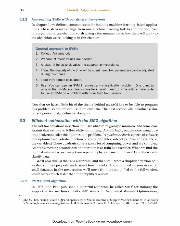
6.2.2 Approaching SVMs with our general frameworkIn chapter 1, we defined common steps for building machine learning–based applica-tions. These steps may change from one machine learning task to another and fromone algorithm to another. It’s worth taking a few minutes to see how these will apply tothe algorithm we’re looking at in this chapter.

Now that we have a little bit of the theory behind us, we’d like to be able to programthis problem so that we can use it on our data. The next section will introduce a sim-ple yet powerful algorithm for doing so.

6.3 Efficient optimization with the SMO algorithm The last two equations in section 6.2.1 are what we’re going to minimize and some con-straints that we have to follow while minimizing. A while back, people were using qua-dratic solvers to solve this optimization problem. (A quadratic solver is a piece of softwarethat optimizes a quadratic function of several variables, subject to linear constraints onthe variables.) These quadratic solvers take a lot of computing power and are complex.All of this messing around with optimization is to train our classifier. When we find theoptimal values of D, we can get our separating hyperplane or line in 2D and then easilyclassify data.

We’ll now discuss the SMO algorithm, and then we’ll write a simplified version of itso that you can properly understand how it works. The simplified version works onsmall datasets. In the next section we’ll move from the simplified to the full version,which works much faster than the simplified version.

6.3.1 Platt’s SMO algorithm

In 1996 John Platt published a powerful algorithm he called SMO3 for training thesupport vector machines. Platt’s SMO stands for Sequential Minimal Optimization,

3 John C. Platt, “Using Analytic QP and Sparseness to Speed Training of Support Vector Machines” in Advancesin Neural Information Processing Systems 11, M. S. Kearns, S. A. Solla, D. A. Cohn, eds (MIT Press, 1999), 557–63.

General approach to SVMs1. Collect: Any method.

2. Prepare: Numeric values are needed.

3. Analyze: It helps to visualize the separating hyperplane.

4. Train: The majority of the time will be spent here. Two parameters can be adjustedduring this phase.

5. Test: Very simple calculation.

6. Use: You can use an SVM in almost any classification problem. One thing tonote is that SVMs are binary classifiers. You’ll need to write a little more codeto use an SVM on a problem with more than two classes.


107Efficient optimization with the SMO algorithm

and it takes the large optimization problem and breaks it into many small problems.The small problems can easily be solved, and solving them sequentially will give youthe same answer as trying to solve everything together. In addition to getting the sameanswer, the amount of time is greatly reduced.

The SMO algorithm works to find a set of alphas and b. Once we have a set ofalphas, we can easily compute our weights w and get the separating hyperplane.

Here’s how the SMO algorithm works: it chooses two alphas to optimize on eachcycle. Once a suitable pair of alphas is found, one is increased and one is decreased.To be suitable, a set of alphas must meet certain criteria. One criterion a pair mustmeet is that both of the alphas have to be outside their margin boundary. The secondcriterion is that the alphas aren’t already clamped or bounded.

6.3.2 Solving small datasets with the simplified SMOImplementing the full Platt SMO algorithm can take a lot of code. We’ll simplify it inour first example to get an idea of how it works. After we get the simplified versionworking, we’ll build on it to see the full version. The simplification uses less code buttakes longer at runtime. The outer loops of the Platt SMO algorithm determine thebest alphas to optimize. We’ll skip that for this simplified version and select pairs ofalphas by first going over every alpha in our dataset. Then, we’ll choose the secondalpha randomly from the remaining alphas. It’s important to note here that wechange two alphas at the same time. We need to do this because we have a constraint:

Changing one alpha may cause this constraint to be violated, so we always change twoat a time.

To do this we’re going to create a helper function that randomly selects one inte-ger from a range. We also need a helper function to clip values if they get too big.These two functions are given in the following listing. Open a text editor and add thecode to svmMLiA.py.

def loadDataSet(fileName): dataMat = []; labelMat = [] fr = open(fileName) for line in fr.readlines(): lineArr = line.strip().split('\t') dataMat.append([float(lineArr[0]), float(lineArr[1])]) labelMat.append(float(lineArr[2])) return dataMat,labelMat

def selectJrand(i,m): j=i while (j==i): j = int(random.uniform(0,m)) return j

def clipAlpha(aj,H,L): if aj > H:

Listing 6.1 Helper functions for the SMO algorithm

ai label i� � 0=�¦



aj = H if L > aj: aj = L return aj

The data that’s plotted in figure 6.3 is available in the file testSet.txt. We’ll use thisdataset to develop the SMO algorithm. The first function in listing 6.1 is our familiarloadDatSet(), which opens up the file and parses each line into class labels, and ourdata matrix.

The next function, selectJrand(), takes two values. The first one, i, is the indexof our first alpha, and m is the total number of alphas. A value is randomly chosen andreturned as long as it’s not equal to the input i.

The last helper function, clipAlpha(), clips alpha values that are greater than H orless than L. These three helper functions don’t do much on their own, but they’ll beuseful in our classifier.

After you’ve entered the code from listing 6.1 and saved it, you can try these outusing the following:

>>> import svmMLiA>>> dataArr,labelArr = svmMLiA.loadDataSet('testSet.txt')>>> labelArr[-1.0, -1.0, 1.0, -1.0, 1.0, 1.0, 1.0, -1.0, -1.0, -1.0, -1.0, -1.0, -1.0, 1.0...

You can see that the class labels are -1 and 1 rather than 0 and 1. Now that we have these working, we’re ready for our first version of the SMO

algorithm. Pseudocode for this function would look like this:

Create an alphas vector filled with 0sWhile the number of iterations is less than MaxIterations:

For every data vector in the dataset: If the data vector can be optimized: Select another data vector at random Optimize the two vectors together If the vectors can’t be optimized ➞ breakIf no vectors were optimized ➞ increment the iteration count

The code in listing 6.2 is a working version of the SMO algorithm. In Python, if we enda line with \, the interpreter will assume the statement is continued on the next line.There are a number of long lines in the following code that need to be broken up, soI’ve used the \ symbol for this. Open the file svmMLiA.py and enter the code from thefollowing listing.

def smoSimple(dataMatIn, classLabels, C, toler, maxIter): dataMatrix = mat(dataMatIn); labelMat = mat(classLabels).transpose() b = 0; m,n = shape(dataMatrix)

Listing 6.2 The simplified SMO algorithm



alphas = mat(zeros((m,1))) iter = 0 while (iter < maxIter): alphaPairsChanged = 0 for i in range(m): fXi = float(multiply(alphas,labelMat).T*\ (dataMatrix*dataMatrix[i,:].T)) + b Ei = fXi - float(labelMat[i]) if ((labelMat[i]*Ei < -toler) and (alphas[i] < C)) or \ ((labelMat[i]*Ei > toler) and \ (alphas[i] > 0)): j = selectJrand(i,m) fXj = float(multiply(alphas,labelMat).T*\ (dataMatrix*dataMatrix[j,:].T)) + b Ej = fXj - float(labelMat[j]) alphaIold = alphas[i].copy(); alphaJold = alphas[j].copy(); if (labelMat[i] != labelMat[j]): L = max(0, alphas[j] - alphas[i]) H = min(C, C + alphas[j] - alphas[i]) else: L = max(0, alphas[j] + alphas[i] - C) H = min(C, alphas[j] + alphas[i]) if L==H: print "L==H"; continue eta = 2.0 * dataMatrix[i,:]*dataMatrix[j,:].T - \ dataMatrix[i,:]*dataMatrix[i,:].T - \ dataMatrix[j,:]*dataMatrix[j,:].T if eta >= 0: print "eta>=0"; continue alphas[j] -= labelMat[j]*(Ei - Ej)/eta alphas[j] = clipAlpha(alphas[j],H,L) if (abs(alphas[j] - alphaJold) < 0.00001): print \ "j not moving enough"; continue alphas[i] += labelMat[j]*labelMat[i]*\ (alphaJold - alphas[j]) b1 = b - Ei- labelMat[i]*(alphas[i]-alphaIold)*\ dataMatrix[i,:]*dataMatrix[i,:].T - \ labelMat[j]*(alphas[j]-alphaJold)*\ dataMatrix[i,:]*dataMatrix[j,:].T b2 = b - Ej- labelMat[i]*(alphas[i]-alphaIold)*\ dataMatrix[i,:]*dataMatrix[j,:].T - \ labelMat[j]*(alphas[j]-alphaJold)*\ dataMatrix[j,:]*dataMatrix[j,:].T if (0 < alphas[i]) and (C > alphas[i]): b = b1 elif (0 < alphas[j]) and (C > alphas[j]): b = b2 else: b = (b1 + b2)/2.0 alphaPairsChanged += 1 print "iter: %d i:%d, pairs changed %d" % \ (iter,i,alphaPairsChanged) if (alphaPairsChanged == 0): iter += 1 else: iter = 0 print "iteration number: %d" % iter return b,alphas

This is one big function, I know. It’s probably the biggest one you’ll see in this book.This function takes five inputs: the dataset, the class labels, a constant C, the tolerance,

Enter optimizationif alphas can be

changed

B

Randomly select second alphaC

Guarantee alphas stay between 0 and C

D

Update i by sameamount as j in

opposite direction

E

Set theconstant term

F



and the maximum number of iterations before quitting. We’ve been building func-tions in this book with a common interface so you can mix and match algorithms anddata sources. This function takes lists and inputs and transforms them into NumPymatrices so that you can simplify many of the math operations. The class labels aretransposed so that you have a column vector instead of a list. This makes the row ofthe class labels correspond to the row of the data matrix. You also get the constants mand n from the shape of the dataMatIn. Finally, you create a column matrix for thealphas, initialize this to zero, and create a variable called iter. This variable will hold acount of the number of times you’ve gone through the dataset without any alphaschanging. When this number reaches the value of the input maxIter, you exit.

In each iteration, you set alphaPairsChanged to 0 and then go through the entireset sequentially. The variable alphaPairsChanged is used to record if the attempt tooptimize any alphas worked. You’ll see this at the end of the loop. First, fXi is calcu-lated; this is our prediction of the class. The error Ei is next calculated based on theprediction and the real class of this instance. If this error is large, then the alpha cor-responding to this data instance can be optimized. This condition is tested B. In theif statement, both the positive and negative margins are tested. In this if statement,you also check to see that the alpha isn’t equal to 0 or C. Alphas will be clipped at 0 orC, so if they’re equal to these, they’re “bound” and can’t be increased or decreased, soit’s not worth trying to optimize these alphas.

Next, you randomly select a second alpha, alpha[j], using the helper functiondescribed in listing 6.1 C. You calculate the “error” for this alpha similar to what youdid for the first alpha, alpha[i]. The next thing you do is make a copy of alpha[i]and alpha[j]. You do this with the copy() method, so that later you can compare thenew alphas and the old ones. Python passes all lists by reference, so you have toexplicitly tell Python to give you a new memory location for alphaIold andalphaJold. Otherwise, when you later compare the new and old values, we won’t seethe change. You then calculate L and H D, which are used for clamping alpha[j]between 0 and C. If L and H are equal, you can’t change anything, so you issue thecontinue statement, which in Python means “quit this loop now, and proceed to thenext item in the for loop.”

Eta is the optimal amount to change alpha[j]. This is calculated in the long lineof algebra. If eta is 0, you also quit the current iteration of the for loop. This step is asimplification of the real SMO algorithm. If eta is 0, there’s a messy way to calculatethe new alpha[j], but we won’t get into that here. You can read Platt’s original paperif you really want to know how that works. It turns out this seldom occurs, so it’s OK ifyou skip it. You calculate a new alpha[j] and clip it using the helper function fromlisting 6.1 and our L and H values.

Next, you check to see if alpha[j] has changed by a small amount. If so, you quitthe for loop. Next, alpha[i] is changed by the same amount as alpha[j] but in theopposite direction E. After you optimize alpha[i] and alpha[j], you set the con-stant term b for these two alphas F.



Finally, you’ve finished the optimization, and you need to take care to make sureyou exit the loops properly. If you’ve reached the bottom of the for loop without hit-ting a continue statement, then you’ve successfully changed a pair of alphas and youcan increment alphaPairsChanged. Outside the for loop, you check to see if anyalphas have been updated; if so you set iter to 0 and continue. You’ll only stop andexit the while loop when you’ve gone through the entire dataset maxIter number oftimes without anything changing.

To see this in action, type in the following:

>>> b,alphas = svmMLiA.smoSimple(dataArr, labelArr, 0.6, 0.001, 40)The output should look something like this:iteration number: 29j not moving enoughiteration number: 30iter: 30 i:17, pairs changed 1j not moving enoughiteration number: 0j not moving enoughiteration number: 1

This will take a few minutes to converge. Once it’s done, you can inspect the results:

>>> bmatrix([[-3.84064413]])

You can look at the alphas matrix by itself, but there’ll be a lot of 0 elements inside. Tosee the number of elements greater than 0, type in the following:

>>> alphas[alphas>0]matrix([[ 0.12735413, 0.24154794, 0.36890208]])

Your results may differ from these because of the random nature of the SMO algo-rithm. The command alphas[alphas>0] is an example of array filtering, which is spe-cific to NumPy and won’t work with a regular list in Python. If you type in alphas>0,you’ll get a Boolean array with a true in every case where the inequality holds. Then,applying this Boolean array back to the original matrix will give you a NumPy matrixwith only the values that are greater than 0.

To get the number of support vectors, type

>>> shape(alphas[alphas>0])To see which points of our dataset are support vectors, type>>> for i in range(100):... if alphas[i]>0.0: print dataArr[i],labelArr[i]

You should see something like the following:

...[4.6581910000000004, 3.507396] -1.0[3.4570959999999999, -0.082215999999999997] -1.0[6.0805730000000002, 0.41888599999999998] 1.0

The original dataset with these points circled is shown in figure 6.4.



Using the previous settings, I ran this 10 times and took the average time. On my humblelaptop this was 14.5 seconds. This wasn’t bad, but this is a small dataset with only 100points. On larger datasets, this would take a long time to converge. In the next sectionwe’re going speed this up by building the full SMO algorithm.

6.4 Speeding up optimization with the full Platt SMOThe simplified SMO works OK on small datasets with a few hundred points but slowsdown on larger datasets. Now that we’ve covered the simplified version, we can moveon to the full Platt version of the SMO algorithm. The optimization portion where wechange alphas and do all the algebra stays the same. The only difference is how weselect which alpha to use in the optimization. The full Platt uses some heuristics thatincrease the speed. Perhaps in the previous section when executing the example yousaw some room for improvement.

The Platt SMO algorithm has an outer loop for choosing the first alpha. This alter-nates between single passes over the entire dataset and single passes over non-boundalphas. The non-bound alphas are alphas that aren’t bound at the limits 0 or C. Thepass over the entire dataset is easy, and to loop over the non-bound alphas we’ll firstcreate a list of these alphas and then loop over the list. This step skips alphas that weknow can’t change.

The second alpha is chosen using an inner loop after we’ve selected the first alpha.This alpha is chosen in a way that will maximize the step size during optimization. Inthe simplified SMO, we calculated the error Ej after choosing j. This time, we’re goingto create a global cache of error values and choose from the alphas that maximize stepsize, or Ei-Ej.

Figure 6.4 SMO sample dataset showing the support vectors circled and the separating hyperplane after the simplified SMO is run on the data


113Speeding up optimization with the full Platt SMO

Before we get into the improvements, we’re going to need to clean up the codefrom the previous section. The following listing has a data structure we’ll use to cleanup the code and three helper functions for caching the E values. Open your text edi-tor and enter the following code.

class optStruct: def __init__(self,dataMatIn, classLabels, C, toler): self.X = dataMatIn self.labelMat = classLabels self.C = C self.tol = toler self.m = shape(dataMatIn)[0] self.alphas = mat(zeros((self.m,1))) self.b = 0 self.eCache = mat(zeros((self.m,2)))

def calcEk(oS, k): fXk = float(multiply(oS.alphas,oS.labelMat).T*\ (oS.X*oS.X[k,:].T)) + oS.b Ek = fXk - float(oS.labelMat[k]) return Ek

def selectJ(i, oS, Ei): maxK = -1; maxDeltaE = 0; Ej = 0 oS.eCache[i] = [1,Ei] validEcacheList = nonzero(oS.eCache[:,0].A)[0] if (len(validEcacheList)) > 1: for k in validEcacheList: if k == i: continue Ek = calcEk(oS, k) deltaE = abs(Ei - Ek) if (deltaE > maxDeltaE): maxK = k; maxDeltaE = deltaE; Ej = Ek return maxK, Ej else: j = selectJrand(i, oS.m) Ej = calcEk(oS, j) return j, Ej

def updateEk(oS, k): Ek = calcEk(oS, k) oS.eCache[k] = [1,Ek]

The first thing you do is create a data structure to hold all of the important values.This is done with an object. You don’t use it for object-oriented programming; it’sused as a data structure in this example. I moved all the data into a structure to savetyping when you pass values into functions. You can now pass in one object. I couldhave done this just as easily with a Python dictionary, but that takes more work tryingto access member variables; compare myObject.X to myObject['X']. To accomplishthis, you create the class optStruct, which only has the init method. In this method,you populate the member variables. All of these are the same as in the simplified SMO

Listing 6.3 Support functions for full Platt SMO

Error cache

B

Inner-loop heuristic

C

Choose j for maximum step size

D



code, but you’ve added the member variable eCache, which is an mx2 matrix B. Thefirst column is a flag bit stating whether the eCache is valid, and the second column isthe actual E value.

The first helper function, calcEk(), calculates an E value for a given alpha andreturns the E value. This was previously done inline, but you must take it out because itoccurs more frequently in this version of the SMO algorithm.

The next function, selectJ(), selects the second alpha, or the inner loop alpha C.Recall that the goal is to choose the second alpha so that we’ll take the maximum stepduring each optimization. This function takes the error value associated with the firstchoice alpha (Ei) and the index i. You first set the input Ei to valid in the cache.Valid means that it has been calculated. The code nonzero(oS.eCache[:,0].A)[0] cre-ates a list of nonzero values in the eCache. The NumPy function nonzero() returns a listcontaining indices of the input list that are—you guessed it—not zero. The nonzero()statement returns the alphas corresponding to non-zero E values, not the Evalues. You loop through all of these values and choose the value that gives you a max-imum change D. If this is your first time through the loop, you randomly select an alpha.There are more sophisticated ways of handling the first-time case, but this works forour purposes.

The last helper function in listing 6.3 is updateEk(). This calculates the error andputs it in the cache. You’ll use this after you optimize alpha values.

The code in listing 6.3 doesn’t do much on its own. But when combined with theoptimization and the outer loop, it forms the powerful SMO algorithm.

Next, I’ll briefly present the optimization routine, to find our decision boundary.Open your text editor and add the code from the next listing. You’ve already seen thiscode in a different format.

def innerL(i, oS): Ei = calcEk(oS, i) if ((oS.labelMat[i]*Ei < -oS.tol) and (oS.alphas[i] < oS.C)) or\ ((oS.labelMat[i]*Ei > oS.tol) and (oS.alphas[i] > 0)): j,Ej = selectJ(i, oS, Ei) alphaIold = oS.alphas[i].copy(); alphaJold = oS.alphas[j].copy(); if (oS.labelMat[i] != oS.labelMat[j]): L = max(0, oS.alphas[j] - oS.alphas[i]) H = min(oS.C, oS.C + oS.alphas[j] - oS.alphas[i]) else: L = max(0, oS.alphas[j] + oS.alphas[i] - oS.C) H = min(oS.C, oS.alphas[j] + oS.alphas[i]) if L==H: print "L==H"; return 0 eta = 2.0 * oS.X[i,:]*oS.X[j,:].T - oS.X[i,:]*oS.X[i,:].T - \ oS.X[j,:]*oS.X[j,:].T if eta >= 0: print "eta>=0"; return 0 oS.alphas[j] -= oS.labelMat[j]*(Ei - Ej)/eta oS.alphas[j] = clipAlpha(oS.alphas[j],H,L) updateEk(oS, j)

Listing 6.4 Full Platt SMO optimization routine

Second-choice heuristic B

Updates Ecache

C



if (abs(oS.alphas[j] - alphaJold) < 0.00001): print "j not moving enough"; return 0 oS.alphas[i] += oS.labelMat[j]*oS.labelMat[i]*\ (alphaJold - oS.alphas[j]) updateEk(oS, i) b1 = oS.b - Ei- oS.labelMat[i]*(oS.alphas[i]-alphaIold)*\ oS.X[i,:]*oS.X[i,:].T - oS.labelMat[j]*\ (oS.alphas[j]-alphaJold)*oS.X[i,:]*oS.X[j,:].T b2 = oS.b - Ej- oS.labelMat[i]*(oS.alphas[i]-alphaIold)*\ oS.X[i,:]*oS.X[j,:].T - oS.labelMat[j]*\ (oS.alphas[j]-alphaJold)*oS.X[j,:]*oS.X[j,:].T if (0 < oS.alphas[i]) and (oS.C > oS.alphas[i]): oS.b = b1 elif (0 < oS.alphas[j]) and (oS.C > oS.alphas[j]): oS.b = b2 else: oS.b = (b1 + b2)/2.0 return 1 else: return 0

The code in listing 6.4 is almost the same as the smoSimple() function given in list-ing 6.2. But it has been written to use our data structure. The structure is passed in asthe parameter oS. The second important change is that selectJ() from listing 6.3 isused to select the second alpha rather than selectJrand()B. Lastly C, you updatethe Ecache after alpha values change. The final piece of code that wraps all of this upis shown in the following listing. This is the outer loop where you select the firstalpha. Open your text editor and add the code from this listing to svmMLiA.py.

def smoP(dataMatIn, classLabels, C, toler, maxIter, kTup=('lin', 0)): oS = optStruct(mat(dataMatIn),mat(classLabels).transpose(),C,toler) iter = 0 entireSet = True; alphaPairsChanged = 0 while (iter < maxIter) and ((alphaPairsChanged > 0) or (entireSet)): alphaPairsChanged = 0 if entireSet: for i in range(oS.m): alphaPairsChanged += innerL(i,oS) print "fullSet, iter: %d i:%d, pairs changed %d" %\ (iter,i,alphaPairsChanged) iter += 1 else: nonBoundIs = nonzero((oS.alphas.A > 0) * (oS.alphas.A < C))[0] for i in nonBoundIs: alphaPairsChanged += innerL(i,oS) print "non-bound, iter: %d i:%d, pairs changed %d" % \ (iter,i,alphaPairsChanged) iter += 1 if entireSet: entireSet = False elif (alphaPairsChanged == 0): entireSet = True print "iteration number: %d" % iter return oS.b,oS.alphas

The code in listing 6.5 is the full Platt SMO algorithm. The inputs are the same as thefunction smoSimple(). Initially you create the data structure that will be used to hold

Listing 6.5 Full Platt SMO outer loop

Updates Ecache

C

Go over all valuesB

Go over non-bound values

C



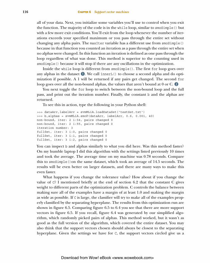
all of your data. Next, you initialize some variables you’ll use to control when you exitthe function. The majority of the code is in the while loop, similar to smoSimple() butwith a few more exit conditions. You’ll exit from the loop whenever the number of iter-ations exceeds your specified maximum or you pass through the entire set withoutchanging any alpha pairs. The maxIter variable has a different use from smoSimple()because in that function you counted an iteration as a pass through the entire set whenno alphas were changed. In this function an iteration is defined as one pass through theloop regardless of what was done. This method is superior to the counting used insmoSimple() because it will stop if there are any oscillations in the optimization.

Inside the while loop is different from smoSimple(). The first for loop goes overany alphas in the dataset B. We call innerL() to choose a second alpha and do opti-mization if possible. A 1 will be returned if any pairs get changed. The second forloop goes over all the non-bound alphas, the values that aren’t bound at 0 or C. C

You next toggle the for loop to switch between the non-bound loop and the fullpass, and print out the iteration number. Finally, the constant b and the alphas arereturned.

To see this in action, type the following in your Python shell:

>>> dataArr,labelArr = svmMLiA.loadDataSet('testSet.txt')>>> b,alphas = svmMLiA.smoP(dataArr, labelArr, 0.6, 0.001, 40)non-bound, iter: 2 i:54, pairs changed 0non-bound, iter: 2 i:55, pairs changed 0iteration number: 3fullSet, iter: 3 i:0, pairs changed 0fullSet, iter: 3 i:1, pairs changed 0fullSet, iter: 3 i:2, pairs changed 0

You can inspect b and alphas similarly to what you did here. Was this method faster?On my humble laptop I did this algorithm with the settings listed previously 10 timesand took the average. The average time on my machine was 0.78 seconds. Comparethis to smoSimple()on the same dataset, which took an average of 14.5 seconds. Theresults will be even better on larger datasets, and there are many ways to make thiseven faster.

What happens if you change the tolerance value? How about if you change thevalue of C? I mentioned briefly at the end of section 6.2 that the constant C givesweight to different parts of the optimization problem. C controls the balance betweenmaking sure all of the examples have a margin of at least 1.0 and making the marginas wide as possible. If C is large, the classifier will try to make all of the examples prop-erly classified by the separating hyperplane. The results from this optimization run areshown in figure 6.5. Comparing figure 6.5 to 6.4 you see that there are more supportvectors in figure 6.5. If you recall, figure 6.4 was generated by our simplified algo-rithm, which randomly picked pairs of alphas. This method worked, but it wasn’t asgood as the full version of the algorithm, which covered the entire dataset. You mayalso think that the support vectors chosen should always be closest to the separatinghyperplane. Given the settings we have for C, the support vectors circled give us a



solution that satisfies the algorithm. When you have a dataset that isn’t linearly separa-ble, you’ll see the support vectors bunch up closer to the hyperplane.

You might be thinking, “We just spent a lot of time figuring out the alphas, but howdo we use this to classify things?” That’s not a problem. You first need to get the hyper-plane from the alphas. This involves calculating ws. The small function listed here willdo that for you:

def calcWs(alphas,dataArr,classLabels): X = mat(dataArr); labelMat = mat(classLabels).transpose() m,n = shape(X) w = zeros((n,1)) for i in range(m): w += multiply(alphas[i]*labelMat[i],X[i,:].T) return w

The most important part of the code is the for loop, which just multiplies some thingstogether. If you looked at any of the alphas we calculated earlier, remember that mostof the alphas are 0s. The non-zero alphas are our support vectors. This for loop goesover all the pieces of data in our dataset, but only the support vectors matter. Youcould just as easily throw out those other data points because they don’t contribute tothe w calculations.

To use the function listed previously, type in the following:

>>> ws=svmMLiA.calcWs(alphas,dataArr,labelArr)>>> wsarray([[ 0.65307162], [-0.17196128]])

Now to classify something, say the first data point, type in this:

>>> datMat=mat(dataArr)>>> datMat[0]*mat(ws)+bmatrix([[-0.92555695]])

Figure 6.5 Support vectors shown af-ter the full SMO algorithm is run on the dataset. The results are slightly differ-ent from those in figure 6.4.



If this value is greater than 0, then its class is a 1, and the class is -1 if it’s less than 0.For point 0 you should then have a label of -1. Check to make sure this is true:

>>> labelArr[0]-1.0

Now check to make sure other pieces of data are properly classified:

>>> datMat[2]*mat(ws)+bmatrix([[ 2.30436336]])>>> labelArr[2]1.0>>> datMat[1]*mat(ws)+bmatrix([[-1.36706674]])>>> labelArr[1]-1.0

Compare these results to figure 6.5 to make sure it makes sense. Now that we can successfully train our classifier, I’d like to point out that the two

classes fit on either side of a straight line. If you look at figure 6.1, you can probablyfind shapes that would separate the two classes. What if you want your classes to beinside a circle or outside a circle? We’ll next talk about a way you can change the clas-sifier to account for different shapes of regions separating your data.

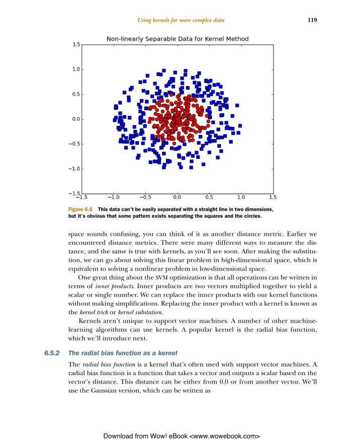
6.5 Using kernels for more complex dataConsider the data in figure 6.6. This is similar to the data in figure 6.1, frame C. Ear-lier, this was used to describe data that isn’t linearly separable. Clearly there’s somepattern in this data that we can recognize. Is there a way we can use our powerful toolsto capture this pattern in the same way we did for the linear data? Yes, there is. We’regoing to use something called a kernel to transform our data into a form that’s easilyunderstood by our classifier. This section will explain kernels and how we can usethem to support vector machines. Next, you’ll see one popular type of kernel calledthe radial bias function, and finally we’ll apply this to our existing classifier.

6.5.1 Mapping data to higher dimensions with kernels

The points in figure 6.1 are in a circle. The human brain can recognize that. Our clas-sifier, on the other hand, can only recognize greater than or less than 0. If we justplugged in our X and Y coordinates, we wouldn’t get good results. You can probablythink of some ways to change the circle data so that instead of X and Y, you’d havesome new variables that would be better on the greater-than- or less-than-0 test. This isan example of transforming the data from one feature space to another so that youcan deal with it easily with your existing tools. Mathematicians like to call this mappingfrom one feature space to another feature space. Usually, this mapping goes from a lower-dimensional feature space to a higher-dimensional space.

This mapping from one feature space to another is done by a kernel. You can thinkof the kernel as a wrapper or interface for the data to translate it from a difficult for-matting to an easier formatting. If this mapping from a feature space to another feature


119Using kernels for more complex data

space sounds confusing, you can think of it as another distance metric. Earlier weencountered distance metrics. There were many different ways to measure the dis-tance, and the same is true with kernels, as you’ll see soon. After making the substitu-tion, we can go about solving this linear problem in high-dimensional space, which isequivalent to solving a nonlinear problem in low-dimensional space.

One great thing about the SVM optimization is that all operations can be written interms of inner products. Inner products are two vectors multiplied together to yield ascalar or single number. We can replace the inner products with our kernel functionswithout making simplifications. Replacing the inner product with a kernel is known asthe kernel trick or kernel substation.

Kernels aren’t unique to support vector machines. A number of other machine-learning algorithms can use kernels. A popular kernel is the radial bias function,which we’ll introduce next.

6.5.2 The radial bias function as a kernel

The radial bias function is a kernel that’s often used with support vector machines. Aradial bias function is a function that takes a vector and outputs a scalar based on thevector’s distance. This distance can be either from 0,0 or from another vector. We’lluse the Gaussian version, which can be written as

Figure 6.6 This data can’t be easily separated with a straight line in two dimensions, but it’s obvious that some pattern exists separating the squares and the circles.



where V is a user-defined parameter that determines the “reach,” or how quickly thisfalls off to 0.

This Gaussian version maps the data from its feature space to a higher featurespace, infinite dimensional to be specific, but don’t worry about that for now. This is acommon kernel to use because you don’t have to figure out exactly how your databehaves, and you’ll get good results with this kernel. In our example we have datathat’s basically in a circle; we could have looked over the data and realized we onlyneeded to measure the distance to the origin; however, if we encounter a new datasetthat isn’t in that format, then we’re in big trouble. We’ll get great results with thisGaussian kernel, and we can use it on many other datasets and get low error ratesthere too.

If you add one function to our svmMLiA.py file and make a few modifications,you’ll be able to use kernels with our existing code. Open your svmMLiA.py code andenter the function kernelTrans(). Also, modify our class, optStruct, so that it lookslike the code given in the following listing.

def kernelTrans(X, A, kTup): m,n = shape(X) K = mat(zeros((m,1))) if kTup[0]=='lin': K = X * A.T elif kTup[0]=='rbf': for j in range(m): deltaRow = X[j,:] - A K[j] = deltaRow*deltaRow.T K = exp(K /(-1*kTup[1]**2)) else: raise NameError('Houston We Have a Problem -- \ That Kernel is not recognized') return K

class optStruct: def __init__(self,dataMatIn, classLabels, C, toler, kTup): self.X = dataMatIn self.labelMat = classLabels self.C = C self.tol = toler self.m = shape(dataMatIn)[0] self.alphas = mat(zeros((self.m,1))) self.b = 0 self.eCache = mat(zeros((self.m,2))) self.K = mat(zeros((self.m,self.m))) for i in range(self.m): self.K[:,i] = kernelTrans(self.X, self.X[i,:], kTup)

I think it’s best to look at our new version of optStruct. This has everything the sameas the previous optStruct with one new input: kTup. This kTup is a generic tuple that

Listing 6.6 Kernel transformation function

k x,y� � x y– 2–

2V2---------------------© ¹¨ ¸§ ·

exp=

Element-wise division

B



contains the information about the kernel. You’ll see this in action in a little bit. At theend of the initialization method a matrix K gets created and then populated by callinga function kernelTrans(). This global K gets calculated once. Then, when you want touse the kernel, you call it. This saves some redundant computations as well.

When the matrix K is being computed, the function kernelTrans() is called multi-ple times. This takes three inputs: two numeric types and a tuple. The tuple kTupholds information about the kernel. The first argument in the tuple is a string describ-ing what type of kernel should be used. The other arguments are optional argumentsthat may be needed for a kernel. The function first creates a column vector and thenchecks the tuple to see which type of kernel is being evaluated. Here, only two choicesare given, but you can expand this to many more by adding in other elif statements.

In the case of the linear kernel, a dot product is taken between the two inputs,which are the full dataset and a row of the dataset. In the case of the radial bias func-tion, the Gaussian function is evaluated for every element in the matrix in the forloop. After the for loop is finished, you apply the calculations over the entire vector.It’s worth mentioning that in NumPy matrices the division symbol means element-wiserather than taking the inverse of a matrix, as would happen in MATLAB. B

Lastly, you raise an exception if you encounter a tuple you don’t recognize. This isimportant because you don’t want the program to continue in this case.

Code was changed to use the kernel functions in two preexisting functions:innerL() and calcEk(). The changes are shown in listing 6.7. I hate to list them outlike this. But relisting the entire functions would take over 90 lines, and I don’t thinkanyone would be happy with that. You can copy the code from the source code down-load to get these changes without manually adding them. Here are the changes:

innerL(): . . .eta = 2.0 * oS.K[i,j] - oS.K[i,i] - oS.K[j,j] . . .b1 = oS.b - Ei- oS.labelMat[i]*(oS.alphas[i]-alphaIold)*oS.K[i,i] -\ oS.labelMat[j]*(oS.alphas[j]-alphaJold)*oS.K[i,j]b2 = oS.b - Ej- oS.labelMat[i]*(oS.alphas[i]-alphaIold)*oS.K[i,j]-\ oS.labelMat[j]*(oS.alphas[j]-alphaJold)*oS.K[j,j] . . .

def calcEk(oS, k): fXk = float(multiply(oS.alphas,oS.labelMat).T*oS.K[:,k] + oS.b) Ek = fXk - float(oS.labelMat[k]) return Ek

Listing 6.7 Changes to innerL() and calcEk() needed to user kernels



Now that you see how to apply a kernel during training, let’s see how you’d use it dur-ing testing.

6.5.3 Using a kernel for testing

We’re going to create a classifier that can properly classify the data points in figure 6.6.We’ll create a classifier that uses the radial bias kernel. The function earlier had oneuser-defined input: V. We need to figure out how big to make this. We’ll create a functionto train and test the classifier using the kernel. The function is shown in the followinglisting. Open your text editor and add in the function testRbf().

def testRbf(k1=1.3): dataArr,labelArr = loadDataSet('testSetRBF.txt') b,alphas = smoP(dataArr, labelArr, 200, 0.0001, 10000, ('rbf', k1)) datMat=mat(dataArr); labelMat = mat(labelArr).transpose() svInd=nonzero(alphas.A>0)[0] sVs=datMat[svInd] labelSV = labelMat[svInd]; print "there are %d Support Vectors" % shape(sVs)[0] m,n = shape(datMat) errorCount = 0 for i in range(m): kernelEval = kernelTrans(sVs,datMat[i,:],('rbf', k1)) predict=kernelEval.T * multiply(labelSV,alphas[svInd]) + b if sign(predict)!=sign(labelArr[i]): errorCount += 1 print "the training error rate is: %f" % (float(errorCount)/m) dataArr,labelArr = loadDataSet('testSetRBF2.txt') errorCount = 0 datMat=mat(dataArr); labelMat = mat(labelArr).transpose() m,n = shape(datMat) for i in range(m): kernelEval = kernelTrans(sVs,datMat[i,:],('rbf', k1)) predict=kernelEval.T * multiply(labelSV,alphas[svInd]) + b if sign(predict)!=sign(labelArr[i]): errorCount += 1 print "the test error rate is: %f" % (float(errorCount)/m)

This code only has one input, and that’s optional. The input is the user-defined vari-able for the Gaussian radial bias function. The code is mostly a collection of stuffyou’ve done before. The dataset is loaded from a file. Then, you run the Platt SMOalgorithm on this, with the option 'rbf' for a kernel.

After the optimization finishes, you make matrix copies of the data to use in matrixmath later, and you find the non-zero alphas, which are our support vectors. You alsotake the labels corresponding to the support vectors and the alphas. Those are theonly values you’ll need to do classification.

The most important lines in this whole listing are the first two lines in the forloops. These show how to classify with a kernel. You first use the kernelTrans() func-tion you used in the structure initialization method. After you get the transformeddata, you do a multiplication with the alphas and the labels. The other important

Listing 6.8 Radial bias test function for classifying with a kernel

Create matrix of support vectors



thing to note in these lines is how you use only the data for the support vectors. Therest of the data can be tossed out.

The second for loop is a repeat of the first one but with a different dataset—thetest dataset. You now can compare how different settings perform on the test set andthe training set.

To test out the code from listing 6.8, enter the following at the Python shell:

>>> reload(svmMLiA)<module 'svmMLiA' from 'svmMLiA.pyc'>>>> svmMLiA.testRbf() . .fullSet, iter: 11 i:497, pairs changed 0fullSet, iter: 11 i:498, pairs changed 0fullSet, iter: 11 i:499, pairs changed 0iteration number: 12there are 27 Support Vectorsthe training error rate is: 0.030000the test error rate is: 0.040000

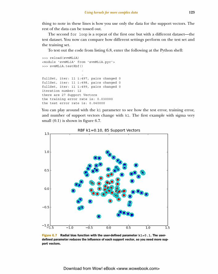
You can play around with the k1 parameter to see how the test error, training error,and number of support vectors change with k1. The first example with sigma verysmall (0.1) is shown in figure 6.7.

Figure 6.7 Radial bias function with the user-defined parameter k1=0.1. The user-defined parameter reduces the influence of each support vector, so you need more sup-port vectors.



In figure 6.7 we have 100 data points, and 85 of them are support vectors. The optimi-zation algorithm found it needed these points in order to properly classify the data.This should give you the intuition that the reach of the radial bias is too small. You canincrease sigma and see how the error rate changes. I increased sigma and madeanother plot, shown in figure 6.8.

Compare figure 6.8 with figure 6.7. Now we have only 27 support vectors. This ismuch smaller. If you watch the output of the function testRbf(), you’ll see that thetest error has gone down too. This dataset has an optimum somewhere around thissetting. If you make the sigma smaller, you’ll get a lower training error but a highertesting error.

There is an optimum number of support vectors. The beauty of SVMs is that theyclassify things efficiently. If you have too few support vectors, you may have a poordecision boundary (this will be demonstrated in the next example). If you have toomany support vectors, you’re using the whole dataset every time you classify some-thing—that’s called k-Nearest Neighbors.

Feel free to play around with other settings in the SMO algorithm or to create newkernels. We’re now going to put our support vector machines to use with some largerdata and compare it with a classifier you saw earlier.

Figure 6.8 Radial bias kernel function with user parameter k1=1.3. Here we have fewer support vectors than in figure 6.7. The support vectors are bunching up around the de-cision boundary.


125Example: revisiting handwriting classification

6.6 Example: revisiting handwriting classificationConsider the following hypothetical situation. Your manager comes to you and says,“That handwriting recognition program you made is great, but it takes up too muchmemory and customers can’t download our application over the air. (At the time ofwriting there’s a 10 MB limit on certain applications downloaded over the air. I’m surethis will be laughable at some point in the future.) We need you to keep the same per-formance with less memory used. I told the CEO you’d have this ready in a week. Howlong will it take?” I’m not sure how you’d respond, but if you wanted to comply withtheir request, you could consider using support vector machines. The k-NearestNeighbors algorithm used in chapter 2 works well, but you have to carry around allthe training examples. With support vector machines, you can carry around far fewerexamples (only your support vectors) and achieve comparable performance.

Using some of the code from chapter 2 and the SMO algorithm, let’s build a system totest a classifier on the handwritten digits. Open svmMLiA.py and copy over the functionimg2vector() from knn.py in chapter 2. Then, add the code in the following listing.

def loadImages(dirName): from os import listdir hwLabels = [] trainingFileList = listdir(dirName) m = len(trainingFileList) trainingMat = zeros((m,1024)) for i in range(m): fileNameStr = trainingFileList[i] fileStr = fileNameStr.split('.')[0] classNumStr = int(fileStr.split('_')[0]) if classNumStr == 9: hwLabels.append(-1) else: hwLabels.append(1) trainingMat[i,:] = img2vector('%s/%s' % (dirName, fileNameStr)) return trainingMat, hwLabels

Listing 6.9 Support vector machine handwriting recognition

Example: digit recognition with SVMs1. Collect: Text file provided.

2. Prepare: Create vectors from the binary images.

3. Analyze: Visually inspect the image vectors.

4. Train: Run the SMO algorithm with two different kernels and different settings forthe radial bias kernel.

5. Test: Write a function to test the different kernels and calculate the error rate.

6. Use: A full application of image recognition requires some image processing,which we won’t get into.



def testDigits(kTup=('rbf', 10)): dataArr,labelArr = loadImages('trainingDigits') b,alphas = smoP(dataArr, labelArr, 200, 0.0001, 10000, kTup) datMat=mat(dataArr); labelMat = mat(labelArr).transpose() svInd=nonzero(alphas.A>0)[0] sVs=datMat[svInd] labelSV = labelMat[svInd]; print "there are %d Support Vectors" % shape(sVs)[0] m,n = shape(datMat) errorCount = 0 for i in range(m): kernelEval = kernelTrans(sVs,datMat[i,:],kTup) predict=kernelEval.T * multiply(labelSV,alphas[svInd]) + b if sign(predict)!=sign(labelArr[i]): errorCount += 1 print "the training error rate is: %f" % (float(errorCount)/m) dataArr,labelArr = loadImages('testDigits') errorCount = 0 datMat=mat(dataArr); labelMat = mat(labelArr).transpose() m,n = shape(datMat) for i in range(m): kernelEval = kernelTrans(sVs,datMat[i,:],kTup) predict=kernelEval.T * multiply(labelSV,alphas[svInd]) + b if sign(predict)!=sign(labelArr[i]): errorCount += 1 print "the test error rate is: %f" % (float(errorCount)/m)

The function loadImages() appeared as part of handwritingClassTest() earlier inkNN.py. It has been refactored into its own function. The only big difference is that inkNN.py this code directly applied the class label. But with support vector machines, youneed a class label of -1 or +1, so if you encounter a 9 it becomes -1; otherwise, the labelis +1. Actually, support vector machines are only a binary classifier. They can onlychoose between +1 and -1. Creating a multiclass classifier with SVMs has been studiedand compared. If you’re interested, I suggest you read a paper called “A Comparison ofMethods for Multiclass Support Vector Machines” by C. W. Hus et al.4 Because we’redoing binary classification, I’ve taken out all of the data except the 1 and 9 digits.

The next function, testDigits(), isn’t super new. It’s almost the exact same codeas testRbf(), except it calls loadImages() to get the class labels and data. The othersmall difference is that the kernel tuple kTup is now an input, whereas it was assumedthat you were using the rbf kernel in testRbf(). If you don’t add any input argumentsto testDigits(), it will use the default of (‘rbf’, 10) for kTup.

After you’ve entered the code from listing 6.9, save svmMLiA.py and type in thefollowing:

>>> svmMLiA.testDigits(('rbf', 20)) . .L==HfullSet, iter: 3 i:401, pairs changed 0iteration number: 4

4 C. W. Hus, and C. J. Lin, “A Comparison of Methods for Multiclass Support Vector Machines,” IEEE Transac-tions on Neural Networks 13, no. 2 (March 2002), 415–25.


127Summary

there are 43 Support Vectorsthe training error rate is: 0.017413the test error rate is: 0.032258

I tried different values for sigma as well as trying the linear kernel and summarizedthem in table 6.1.

The results in table 6.1 show that we achieve a minimum test error with the radial biasfunction kernel somewhere around 10. This is much larger than our previous exam-ple, where our minimum test error was roughly 1.3. Why is there such a huge differ-ence? The data is different. In the handwriting data, we have 1,024 features that couldbe as high as 1.0. In the example in section 6.5, our data varied from -1 to 1, but wehad only two features. How can you tell what settings to use? To be honest, I didn’tknow when I was writing this example. I just tried some different settings. The answeris also sensitive to the settings of C. There are other formulations of the SVM thatbring C into the optimization procedure, such as v-SVM. A good discussion aboutv-SVM can be found in chapter 3 of Pattern Recognition, by Sergios Theodoridis andKonstantinos Koutroumbas.5

It’s interesting to note that the minimum training error doesn’t correspond to aminimum number of support vectors. Also note that the linear kernel doesn’t haveterrible performance. It may be acceptable to trade the linear kernel’s error rate forincreased speed of classification, but that depends on your application.

6.7 SummarySupport vector machines are a type of classifier. They’re called machines because theygenerate a binary decision; they’re decision machines. Support vectors have good gen-eralization error: they do a good job of learning and generalizing on what they’velearned. These benefits have made support vector machines popular, and they’re con-sidered by some to be the best stock algorithm in unsupervised learning.

Table 6.1 Handwritten digit performance for different kernel settings

Kernel, settings Training error (%) Test error (%) # Support vectors

RBF, 0.1 0 52 402

RBF, 5 0 3.2 402

RBF, 10 0 0.5 99

RBF, 50 0.2 2.2 41

RBF, 100 4.5 4.3 26

Linear 2.7 2.2 38

5 Sergios Theodoridis and Konstantinos Koutroumbas, Pattern Recognition, 4th ed. (Academic Press, 2009), 133.



Support vector machines try to maximize margin by solving a quadratic optimiza-tion problem. In the past, complex, slow quadratic solvers were used to train supportvector machines. John Platt introduced the SMO algorithm, which allowed fast train-ing of SVMs by optimizing only two alphas at one time. We discussed the SMO optimi-zation procedure first in a simplified version. We sped up the SMO algorithm a lot byusing the full Platt version over the simplified version. There are many furtherimprovements that you could make to speed it up even further. A commonly cited ref-erence for further speed-up is the paper titled “Improvements to Platt’s SMO Algo-rithm for SVM Classifier Design.”6

Kernel methods, or the kernel trick, map data (sometimes nonlinear data) from alow-dimensional space to a high-dimensional space. In a higher dimension, you cansolve a linear problem that’s nonlinear in lower-dimensional space. Kernel methodscan be used in other algorithms than just SVM. The radial-bias function is a popularkernel that measures the distance between two vectors.

Support vector machines are a binary classifier and additional methods can beextended to classification of classes greater than two. The performance of an SVM isalso sensitive to optimization parameters and parameters of the kernel used.

Our next chapter will wrap up our coverage of classification by focusing on some-thing called boosting. A number of similarities can be drawn between boosting and sup-port vector machines, as you’ll soon see.

6 S. S. Keerthi, S. K. Shevade, C. Bhattacharyya, and K. R. K. Murthy, “Improvements to Platt’s SMO Algorithmfor SVM Classifier Design,” Neural Computation 13, no. 3,( 2001), 637–49.


Documents

Support vector machines - ccs.neu.edu