Embed Size (px)
Citation preview

Support Vector Machines
Charlie Frogner 1
MIT
2011
1Slides mostly stolen from Ryan Rifkin (Google).C. Frogner Support Vector Machines

Plan
Regularization derivation of SVMs.
Analyzing the SVM problem: optimization, duality.
Geometric derivation of SVMs.
Practical issues.
C. Frogner Support Vector Machines

The Regularization Setting (Again)
Given n examples (x1, y1), . . . , (xn, yn), with xi ∈ Rn and
yi ∈ {−1,1} for all i .We can find a classification function by solving a regularizedlearning problem:
argminf∈H
1n
n∑
i=1
V (yi , f (xi)) + λ||f ||2H.
Note that in this class we are specifically considering binaryclassification .
C. Frogner Support Vector Machines
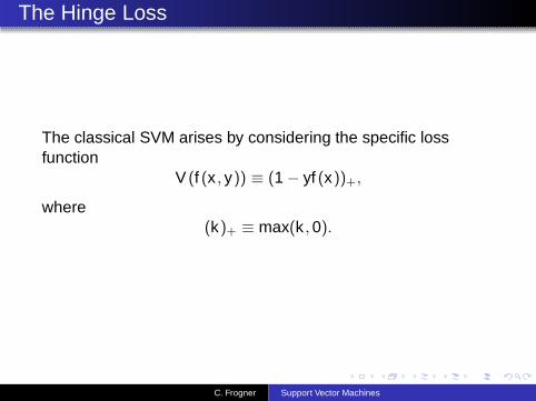
The Hinge Loss
The classical SVM arises by considering the specific lossfunction
V (f (x , y)) ≡ (1 − yf (x))+,
where(k)+ ≡ max(k ,0).
C. Frogner Support Vector Machines
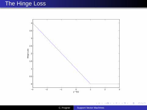
The Hinge Loss
−3 −2 −1 0 1 2 3
0
0.5
1
1.5
2
2.5
3
3.5
4
y * f(x)
Hin
ge L
oss
C. Frogner Support Vector Machines
Substituting In The Hinge Loss
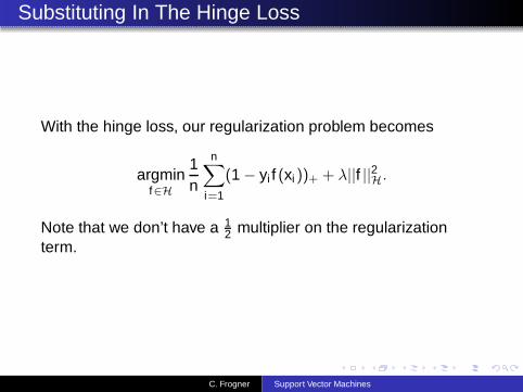
With the hinge loss, our regularization problem becomes
argminf∈H
1n
n∑
i=1
(1 − yi f (xi ))+ + λ||f ||2H.
Note that we don’t have a 12 multiplier on the regularization
term.
C. Frogner Support Vector Machines

Slack Variables
This problem is non-differentiable (because of the “kink” in V ).So rewrite the “max” function using slack variables ξi .
argminf∈H
1n
∑ni=1 ξi + λ||f ||2H
subject to : ξi ≥ 1 − yi f (xi) i = 1, . . . ,n
ξi ≥ 0 i = 1, . . . ,n
C. Frogner Support Vector Machines
Applying The Representer Theorem
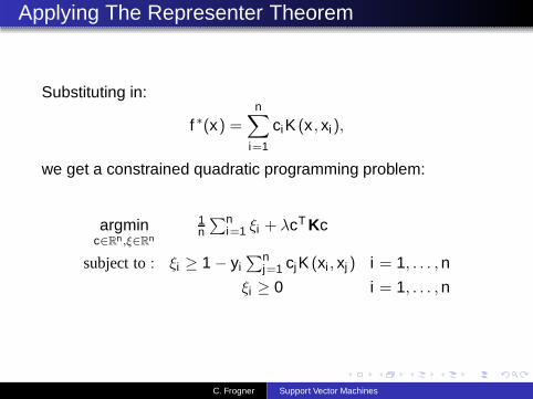
Substituting in:
f ∗(x) =n
∑
i=1
ciK (x , xi),
we get a constrained quadratic programming problem:
argminc∈Rn ,ξ∈Rn
1n
∑ni=1 ξi + λcT Kc
subject to : ξi ≥ 1 − yi∑n
j=1 cjK (xi , xj ) i = 1, . . . ,n
ξi ≥ 0 i = 1, . . . ,n
C. Frogner Support Vector Machines
Adding A Bias Term
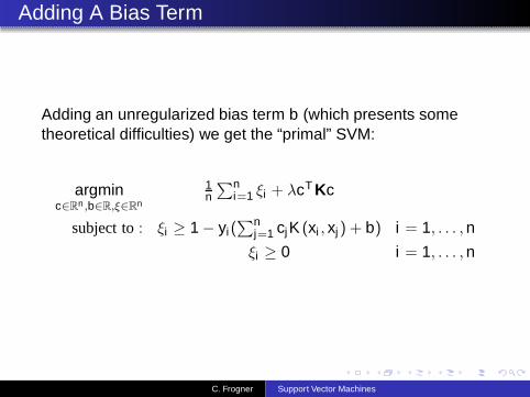
Adding an unregularized bias term b (which presents sometheoretical difficulties) we get the “primal” SVM:
argminc∈Rn ,b∈R,ξ∈Rn
1n
∑ni=1 ξi + λcT Kc
subject to : ξi ≥ 1 − yi(∑n
j=1 cjK (xi , xj ) + b) i = 1, . . . ,n
ξi ≥ 0 i = 1, . . . ,n
C. Frogner Support Vector Machines

Standard Notation
In most of the SVM literature, instead of λ, a parameter C isused to control regularization:
C =1
2λn.
Using this definition (after multiplying our objective function bythe constant 1
2λ , the regularization problem becomes
argminf∈H
Cn
∑
i=1
V (yi , f (xi )) +12||f ||2H.
Like λ, the parameter C also controls the tradeoff betweenclassification accuracy and the norm of the function. The primalproblem becomes . . .
C. Frogner Support Vector Machines

The Reparametrized Problem
argminc∈Rn ,b∈R,ξ∈Rn
C∑n
i=1 ξi +12cT Kc
subject to : ξi ≥ 1 − yi(∑n
j=1 cjK (xi , xj ) + b) i = 1, . . . ,n
ξi ≥ 0 i = 1, . . . ,n
C. Frogner Support Vector Machines

How to Solve?
argminc∈Rn ,b∈R,ξ∈Rn
C∑n
i=1 ξi +12cT Kc
subject to : ξi ≥ 1 − yi(∑n
j=1 cjK (xi , xj ) + b) i = 1, . . . ,n
ξi ≥ 0 i = 1, . . . ,n
This is a constrained optimization problem. The generalapproach:
Form the primal problem – we did this.Lagrangian from primal – just like Lagrange multipliers.Dual – one dual variable associated to each primalconstraint in the Lagrangian.
C. Frogner Support Vector Machines
Lagrangian
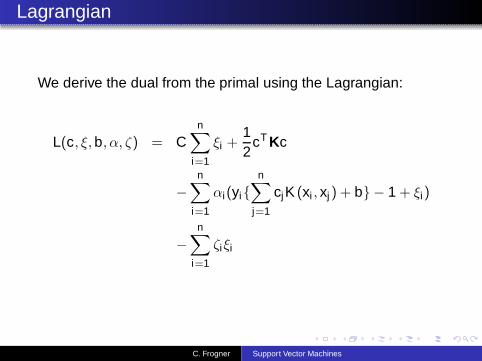
We derive the dual from the primal using the Lagrangian:
L(c, ξ,b, α, ζ) = Cn
∑
i=1
ξi +12
cT Kc
−
n∑
i=1
αi(yi{
n∑
j=1
cjK (xi , xj ) + b} − 1 + ξi)
−
n∑
i=1
ζiξi
C. Frogner Support Vector Machines

Dual I
Dual problem is:
argmaxα,ζ≥0
infc,ξ,b
L(c, ξ,b, α, ζ)
First, minimize L w.r.t. (c, ξ,b):
(1) ∂L∂c = 0 =⇒ ci = αiyi
(2) ∂L∂b = 0 =⇒
n∑
i=1
αiyi = 0
(3) ∂L∂ξi
= 0 =⇒ C − αi − ζi = 0
=⇒ 0 ≤ αi ≤ C
C. Frogner Support Vector Machines
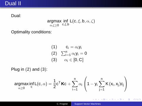
Dual II
Dual:argmaxα,ζ≥0
infc,ξ,b
L(c, ξ,b, α, ζ)
Optimality conditions:
(1) ci = αiyi
(2)∑n
i=1 αiyi = 0
(3) αi ∈ [0,C]
Plug in (2) and (3):
argmaxα≥0
infc
L(c, α) =12
cT Kc +n
∑
i=1
αi
1 − yi
n∑
j=1
K (xi , xj )cj
C. Frogner Support Vector Machines

Dual II
Dual:argmaxα,ζ≥0
infc,ξ,b
L(c, ξ,b, α, ζ)
Optimality conditions:
(1) ci = αiyi
(2)∑n
i=1 αiyi = 0
(3) αi ∈ [0,C]
Plug in (1):
argmaxα≥0
L(α) =∑n
i=1 αi −12
∑ni ,j=1 αiyiK (xi , xj)αjyj
=∑n
i=1 αi −12α
T (diagY)K(diagY)α
C. Frogner Support Vector Machines

The Primal and Dual Problems Again
argminc∈Rn ,b∈R,ξ∈Rn
C∑n
i=1 ξi +12cT Kc
subject to : ξi ≥ 1 − yi(∑n
j=1 cjK (xi , xj ) + b) i = 1, . . . ,n
ξi ≥ 0 i = 1, . . . ,n
maxα∈Rn
∑ni=1 αi −
12α
T Qα
subject to :∑n
i=1 yiαi = 0
0 ≤ αi ≤ C i = 1, . . . ,n
C. Frogner Support Vector Machines

SVM Training
Basic idea: solve the dual problem to find the optimal α’s,and use them to find b and c.
The dual problem is easier to solve the primal problem. Ithas simple box constraints and a single equality constraint,and the problem can be decomposed into a sequence ofsmaller problems (see appendix).
C. Frogner Support Vector Machines

Interpreting the solution
α tells us:
c and b.
The identities of the misclassified points.
How to analyze? Use the optimality conditions.
Already used: derivative of L w.r.t. (c, ξ,b) is zero atoptimality.
Haven’t used: complementary slackness, primal/dualconstraints.
C. Frogner Support Vector Machines
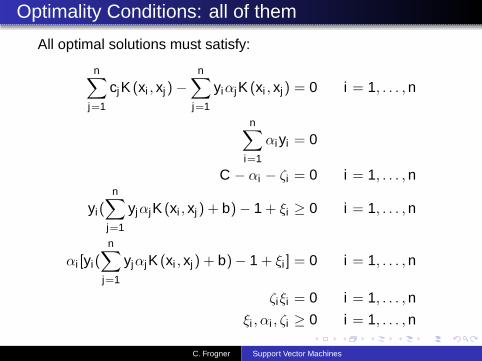
Optimality Conditions: all of them
All optimal solutions must satisfy:
n∑
j=1
cjK (xi , xj)−n
∑
j=1
yiαjK (xi , xj) = 0 i = 1, . . . ,n
n∑
i=1
αiyi = 0
C − αi − ζi = 0 i = 1, . . . ,n
yi(n
∑
j=1
yjαjK (xi , xj ) + b)− 1 + ξi ≥ 0 i = 1, . . . ,n
αi [yi(
n∑
j=1
yjαjK (xi , xj) + b)− 1 + ξi ] = 0 i = 1, . . . ,n
ζiξi = 0 i = 1, . . . ,n
ξi , αi , ζi ≥ 0 i = 1, . . . ,n
C. Frogner Support Vector Machines
Optimality Conditions II
These optimality conditions are both necessary and sufficientfor optimality: (c, ξ,b, α, ζ) satisfy all of the conditions if andonly if they are optimal for both the primal and the dual. (Alsoknown as the Karush-Kuhn-Tucker (KKT) conditons.)
C. Frogner Support Vector Machines

Interpreting the solution — c
∂L∂c
= 0 =⇒ ci = αiyi , ∀i
C. Frogner Support Vector Machines

Interpreting the solution — b
Suppose we have the optimal αi ’s. Also suppose that thereexists an i satisfying 0 < αi < C. Then
αi < C =⇒ ζi > 0
=⇒ ξi = 0
=⇒ yi(n
∑
j=1
yjαjK (xi , xj) + b)− 1 = 0
=⇒ b = yi −n
∑
j=1
yjαjK (xi , xj)
C. Frogner Support Vector Machines

Interpreting the solution — sparsity
(Remember we defined f (x) =∑n
i=1 yiαiK (x , xi ) + b.)
yi f (xi) > 1 ⇒ (1 − yi f (xi)) < 0
⇒ ξi 6= (1 − yi f (xi))
⇒ αi = 0
C. Frogner Support Vector Machines

Interpreting the solution —- support vectors
yi f (xi) < 1 ⇒ (1 − yi f (xi)) > 0
⇒ ξi > 0
⇒ ζi = 0
⇒ αi = C
C. Frogner Support Vector Machines

Interpreting the solution — support vectors
Soyi f (xi) < 1 ⇒ αi = C.
Conversely, suppose αi = C:
αi = C =⇒ ξi = 1 − yi f (xi)
=⇒ yi f (xi) ≤ 1
C. Frogner Support Vector Machines

Interpreting the solution
Here are all of the derived conditions:
αi = 0 =⇒ yi f (xi ) ≥ 1
0 < αi < C =⇒ yi f (xi ) = 1
αi = C ⇐= yi f (xi ) < 1
αi = 0 ⇐= yi f (xi ) > 1
αi = C =⇒ yi f (xi ) ≤ 1
C. Frogner Support Vector Machines

Geometric Interpretation of Reduced OptimalityConditions
C. Frogner Support Vector Machines

Summary so far
The SVM is a Tikhonov regularization problem, using thehinge loss:
argminf∈H
1n
n∑
i=1
(1 − yi f (xi))+ + λ||f ||2H.
Solving the SVM means solving a constrained quadraticprogram.
Solutions can be sparse – some coefficients are zero.
The nonzero coefficients correspond to points that aren’tclassified correctly enough – this is where the “supportvector” in SVM comes from.
C. Frogner Support Vector Machines
The Geometric Approach
The “traditional” approach to developing the mathematics ofSVM is to start with the concepts of separating hyperplanesand margin. The theory is usually developed in a linear space,beginning with the idea of a perceptron, a linear hyperplanethat separates the positive and the negative examples. Definingthe margin as the distance from the hyperplane to the nearestexample, the basic observation is that intuitively, we expect ahyperplane with larger margin to generalize better than onewith smaller margin.
C. Frogner Support Vector Machines

Large and Small Margin Hyperplanes
(a) (b)
C. Frogner Support Vector Machines
Maximal Margin Classification
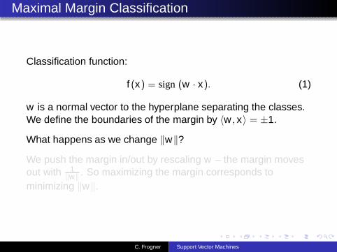
Classification function:
f (x) = sign (w · x). (1)
w is a normal vector to the hyperplane separating the classes.We define the boundaries of the margin by 〈w , x〉 = ±1.
What happens as we change ‖w‖?
We push the margin in/out by rescaling w – the margin movesout with 1
‖w‖ . So maximizing the margin corresponds tominimizing ‖w‖.
C. Frogner Support Vector Machines
Maximal Margin Classification
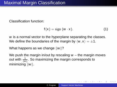
Classification function:
f (x) = sign (w · x). (1)
w is a normal vector to the hyperplane separating the classes.We define the boundaries of the margin by 〈w , x〉 = ±1.
What happens as we change ‖w‖?
We push the margin in/out by rescaling w – the margin movesout with 1
‖w‖ . So maximizing the margin corresponds tominimizing ‖w‖.
C. Frogner Support Vector Machines

Maximal Margin Classification, Separable case
Separable means ∃w s.t. all points are beyond the margin, i.e.
yi〈w , xi〉 ≥ 1 , ∀i .
So we solve:
argminw
‖w‖2
s.t. yi〈w , xi 〉 ≥ 1 , ∀i
C. Frogner Support Vector Machines

Maximal Margin Classification, Non-separable case
Non-separable means there are points on the wrong side of themargin, i.e.
∃i s.t. yi〈w , xi 〉 < 1 .
We add slack variables to account for the wrongness:
argminξi ,w
∑ni=1 ξi + ‖w‖2
s.t. yi〈w , xi〉 ≥ 1 − ξi , ∀i
C. Frogner Support Vector Machines

Historical Perspective
Historically, most developments begin with the geometric form,derived a dual program which was identical to the dual wederived above, and only then observed that the dual programrequired only dot products and that these dot products could bereplaced with a kernel function.
C. Frogner Support Vector Machines

More Historical Perspective
In the linearly separable case, we can also derive theseparating hyperplane as a vector parallel to the vectorconnecting the closest two points in the positive and negativeclasses, passing through the perpendicular bisector of thisvector. This was the “Method of Portraits”, derived by Vapnik inthe 1970’s, and recently rediscovered (with non-separableextensions) by Keerthi.
C. Frogner Support Vector Machines
Summary
The SVM is a Tikhonov regularization problem, with thehinge loss:
argminf∈H
1n
n∑
i=1
(1 − yi f (xi))+ + λ||f ||2H.
Solving the SVM means solving a constrained quadraticprogram.
It’s better to work with the dual program.
Solutions can be sparse – few non-zero coefficients.
The non-zero coefficients correspond to points notclassified correctly enough – a.k.a. “support vectors.”
There is alternative, geometric interpretation of the SVM,from the perspective of “maximizing the margin.”
C. Frogner Support Vector Machines

Practical issues
We can also use RLS for classification. What are thetradeoffs?
SVM possesses sparsity: can have parameters set to zeroin the solution. This enables potentially faster training andfaster prediction than RLS.
SVM QP solvers tend to have many parameters to tune.
SVM can scale to very large datasets, unlike RLS – for themoment (active research topic!).
C. Frogner Support Vector Machines

Good Large-Scale SVM Solvers
SVM Light: http://svmlight.joachims.org
SVM Torch: http://www.torch.ch
libSVM:http://www.csie.ntu.edu.tw/~cjlin/libsvm/
C. Frogner Support Vector Machines

Appendix
(Follows.)
C. Frogner Support Vector Machines
SVM Training
Our plan will be to solve the dual problem to find the α’s, anduse that to find b and our function f . The dual problem is easierto solve the primal problem. It has simple box constraints and asingle inequality constraint, even better, we will see that theproblem can be decomposed into a sequence of smallerproblems.
C. Frogner Support Vector Machines
Off-the-shelf QP software
We can solve QPs using standard software. Many codes areavailable. Main problem — the Q matrix is dense, and isn-by-n, so we cannot write it down. Standard QP softwarerequires the Q matrix, so is not suitable for large problems.
C. Frogner Support Vector Machines

Decomposition, I
Partition the dataset into a working set W and the remainingpoints R. We can rewrite the dual problem as:
maxαW∈R|W |, αR∈R|R|
∑ni=1i∈W
αi +∑
i=1i∈R
αi
−12 [αW αR ]
[
QWW QWR
QRW QRR
] [
αW
αR
]
subject to :∑
i∈W yiαi +∑
i∈R yiαi = 0
0 ≤ αi ≤ C, ∀i
C. Frogner Support Vector Machines

Decomposition, II
Suppose we have a feasible solution α. We can get a bettersolution by treating the αW as variable and the αR as constant.We can solve the reduced dual problem:
maxαW ∈R|W |
(1 − QWRαR)αW − 12αW QWWαW
subject to :∑
i∈W yiαi = −∑
i∈R yiαi
0 ≤ αi ≤ C, ∀i ∈ W
C. Frogner Support Vector Machines
Decomposition, III
The reduced problems are fixed size, and can be solved usinga standard QP code. Convergence proofs are difficult, but thisapproach seems to always converge to an optimal solution inpractice.
C. Frogner Support Vector Machines

Selecting the Working Set
There are many different approaches. The basic idea is toexamine points not in the working set, find points which violatethe reduced optimality conditions, and add them to the workingset. Remove points which are in the working set but are farfrom violating the optimality conditions.
C. Frogner Support Vector Machines