Embed Size (px)
Citation preview

Supply chain coordination with information
sharing in the presence of trust and trustworthiness: a behavioral model from
Guido Voigt
FEMM Working Paper No. 06, March 2009
OTTO-VON-GUERICKE-UNIVERSITY MAGDEBURG FACULTY OF ECONOMICS AND MANAGEMENT
F E M M Faculty of Economics and Management Magdeburg
Working Paper Series
Otto-von-Guericke-University Magdeburg Faculty of Economics and Management
P.O. Box 4120 39016 Magdeburg, Germany
http://www.ww.uni-magdeburg.de/
Supply chain coordination with information
sharing in the presence of trust and
trustworthiness: a behavioral model
Guido Voigt
Otto-von-Guericke-University Magdeburg
Faculty of Economics and Management
Chair of Production and Logistics
POB 4120, 39106 Magdeburg, Germany
Phone: +49 391 / 67 187 86
Abstract
The strategic use of private information causes efficiency losses in traditional principal-agent
settings. One stream of research states that these efficiency losses cannot be overcome if all
agents use their private information strategically. Yet, another stream of research highlights
the importance of communication, trust and trustworthiness in supply chain management. The
underlying work links the concepts of communication, trust and trustworthiness to a
traditional principal-agent setting in a supply chain environment. Surprisingly, it can be
shown that communication and trust can actually lead to increasing efficiency losses although
there is a substantial level of trustworthiness.

- 1 -
Supplier (Principal)
Buyer (Agent)
(honest agent) (deceptive agent)
1 Introduction
Previous research on supply chain coordination shows that a supply chain optimal solution
(i.e. the solution that maximizes the sum of all net present values of the supply chain
members) is typically not achieved as long as the incentives of the independent companies
within the supply chain are not aligned (see e.g. Cachon, 2003). The research field of supply
chain coordination identifies the supply chain optimal solution (e.g. Kelle and Akbulut, 2005)
as well as coordination instruments (e.g. contracts) that align the incentives of the supply
chain members (see e.g. Cachon, 2003).
Earlier work on supply chain coordination demonstrates that asymmetric information are a
major source of inefficiencies within the supply chain, because the strategic use of private
information (e.g. private cost or demand information) can lead to inefficient allocations1,
even though sophisticated menu of contracts (i.e. screening contracts) are utilized (see Corbett
and de Groote, 2000, Ha, 2000, Corbett, 2001, Corbett and Tang, 2003, Corbett et al., 2004,
Sucky, 2004).
The basic idea behind this menu of contracts stems from the revelation principle (see
Myerson, 1986). The specific incentive structure of these contracts ensures that the holder of
the private information does reveal his information by his contract choice. However, as the
contract choice determines the respective supply chain performance, the information revealed
by the contract choice cannot be utilized to design supply chain optimal contracts.
Another stream of research highlights that successful supply chain management and
coordination requires communication (e.g. Cachon and Fisher, 2000) and trust (Moore, 1998
and Zaheer et al., 1998). However, in these studies the incentives for communication and trust
are not explicitly modeled. The goal of this paper is therefore to investigate, under which
circumstances regarding trust and trustworthiness communication is an appropriate
coordination instrument when screening contracts are used.
1 Obviously, private information does not harm supply chain performance, as long as the private information is not decision relevant.
Figure 1: Supply chain configuration

- 2 -
The model utilized in the underlying study captures a supply chain lotsizing decision under
deterministic demand. In a standard principal-agent setting an agent (buyer) holds private
information about her respective holding cost. The principal (supplier) tries to induce higher
order sizes while compensating the buyer for her holding cost increase with a discount on the
purchase price. However, the buyer’s cost increase depends on her holding costs, which are
private information. It is assumed that communication takes place via a signal (e.g. verbal or
written). Standard-theory assumes that the buyer claims a very high compensation (e.g.
quantity discount) for agreeing upon higher order sizes. As the supplier anticipates this
behavior, he will simply ignore the buyer’s signals. The buyer, in turn, anticipates that her
signal has no impact on her profits. Therefore, even the randomization of signals is an
equilibrium strategy. Thus, communication is regarded as cheap-talk and the supply chain
members are caught in a “babbling-equilibrium”. In this case, the supplier’s best action is to
offer a menu of contracts, which leads to inefficient allocations.
However, there is a vast amount of experimental research that shows that cheap talk can
influence the behavior of a decision maker. It is referred to Crawford (1998) for a
comprehensive review of these cheap talk experiments. Particularly, the underlying study is
motivated by the experimental finding from Inderfurth et al. (2008) as well as Özer et al.
(2008) that not all agents use their information entirely strategically. Their findings indicate
that there are different types of agents, who can be divided into two subclasses.
One group includes those agents who always communicate their private information
truthfully. One explanation for this is, for example, that the honest agent faces intrinsic costs
of lying (see Minkler and Miceli, 2004). In the following, these agents are denoted as ‘honest
agents’.
On the other hand there are the agents who misrepresent their private information at least
sometimes. The behavior of these “deceptive agents” may have different explanations. In the
first part of the analysis it is assumed that the deceptive agent does not consider that the
principal might take the signals into account while offering the contracts. In this case the
‘deceptive agent’ is assumed to give signals which do not depend on the private information,
e.g. she unconditionally randomizes the signal. This is the well-known ‘cheap-talk’
hypothesis. In the second part of the analysis we assume that the deceptive agent follows a
strategy which is conditioned on her specific private information.
The remainder of the study is organized as follows: section 2 gives a brief literature review on
the concepts trust, trustworthiness and communication. Section 3 gives an introduction to the

- 3 -
screening-model, which is used as a starting point of the underlying study. Section 4 expands
the scope of the basic model to the possibility of communication. Furthermore, section 4
shows that the supplier can update his expectations on the signals sent by the buyer. Section 5
and 6 evaluate the impact of this adjustment of beliefs on the buyer’s, supplier’s and overall
supply chain’s performance under the unconditional as well as the conditional signaling
assumption, respectively. Finally, Section 7 summarizes the results and gives an outlook for
further research. Please note that the notation is summarized in appendix 9.2.
2 Literature Review
Honest and deceptive agents:
One of the main assumptions of this study is the division of agents into two subclasses. This
assumption has already been made in a similar principal-agent framework from Severinov and
Deneckere (2006). In this study, it is assumed that one subclass of agents is fully rational and
opportunistic. They claim, for example, the highest compensation regardless of their true
holding cost parameter. On the other hand there is a second subclass of agents who will
always communicate their true holding cost, even though they are aware of loosing money by
doing this.
Severinov and Deneckere (2006) utilize the fact, that the deceptive agents can be detected, as
they will give the same signal, e.g. they will always claim the highest possible compensation.
On the other hand, the “honest agents” can be easily identified by a deviation from this
behavior. Every agent who does not claim the highest compensation is therefore identified as
an honest agent. Severinov and Deneckere (2006) propose a “password”-mechanism, where
the password is the signal, which are the deceptive agents supposed to give. Thus, the agent
who knows the password (i.e. the deceptive agent) is offered a more favorable contract than
the honest agent, who does not know the password. However, previous research from Özer et
al. (2008) and Inderfurth et al. (2008) show that even this division in two subgroups may not
be sufficient.
Özer et al. (2008) investigate whether information sharing enhances supply chain
performance in a supplier-manufacturer supply chain with uncertain end-customer demand. A
simple wholesale price contract determines the financial payments in the relationship. In this
study, the supplier’s capacity reservation for the manufacturer relies on a demand forecast.
However, as the manufacturer is closer to the market, she has more accurate forecast
information than the supplier. Under these circumstances, the supply chain optimal solution is

- 4 -
achieved, if the manufacturer reports the demand forecast truthfully. Yet, rational game theory
predicts that the manufacturer exaggerates the demand forecast to influence the supplier’s
capacity reservation decision. In turn, the supplier treats the manufacturer’s information about
the demand forecast as cheap talk.
Interestingly, Özer et al. show in their experiment that the manufacturers inflate the superior
forecast information indeed, but they do not exaggerate to the maximum extent. Particularly,
the report does linearly depend on the private forecast information. The supplier, in turn, does
not treat the report as cheap talk but conditions his capacity decision on the report instead.
Özer et al., thus, find partially trust and trustworthiness in their supply chain setting. This
leads to a higher supply chain performance than theoretically predicted.
Another experimental investigation that analyses the impact of information sharing on supply
chain performance was conducted by Inderfurth et al. (2008). They investigate a stylized joint
economic lot sizing model in a supplier-buyer relationship. In this relationship the buyer holds
private information about her holding cost. The supplier tries to induce higher order sizes
while compensating the buyer for her holding cost increase. In comparison to Özer et al., they
investigate a screening contract instead of the wholesale price contract. They show that buyers
either tend to exaggerate their holding costs or to report them truthfully. However, they also
find that a non negligible portion of reports that understated the respective holding cost.
Additionally, only 1 out of 24 buyers was claiming the highest compensation throughout the
experiment. Finally, they find an ambiguous effect of communication on the overall supply
chain performance. Particularly, the supply chains which manage to build up trust and
trustworthiness performed significantly better than the supply chains in which deception and
strategic interpretation of reports were prevalent.
Taking these behavioral findings into account, the password-mechanism from Severinov and
Deneckere is not applicable as the deceptive agents do not constantly give the same signal
(i.e. always exaggerating to the maximum extent). Hence, the underlying study does not
assume that the deceptive agents are completely strategic. In fact, the deceptive agents are
characterized by signals which are not constantly truthful.
Summarizing the above arguments, the underlying study proposes a behavioral model that
evaluates the impact of trust and communication in a standard principal-agent setting where
the deceptive agents cannot be easily identified by their signals.
- 5 -
Other studies that incorporate the idea of honest and deceptive agents can be found in Alger
and Renault (2005, 2006). However, in contrast to the underlying study there is no direct
communication between the principal and the agent.
Communication:
In Supply Chain Management, information sharing is regarded as one of the main drivers to
improve or even optimize the overall supply chain performance. Chen (2003) gives a
comprehensive review on the potential gains from upstream and downstream sharing of
information such as demand, cost or capacity information. Furthermore, he describes the
screening mechanism, which is utilized in the underlying study, as an enabler to align the
incentives for information sharing.
Mohr and Spekman (1994) find that there are basically three dimensions of communication
behavior that are important to determine the effectiveness of communication in a relationship.
One dimension includes all aspects which refer to the quality of the conveyed information
such as adequacy, accuracy or timeliness. Another dimension includes the degree of which
the communication is “bilateral”, i.e. to what extent both parties within the relationship
consider the shared information in joint decision making. Finally, one dimension includes the
frequency and extent of information sharing. Mohr and Spekman find that all these
dimensions are critical levers to enhance successful partnerships.
In the underlying study it is assumed that all communication fulfills certain quality standards.
This is ensured by restricting the buyer’s signal space to only relevant information.
Furthermore, we assume a strict sequence of events. This ensures the timeliness of
communication. Additionally, it is assumed that the supply chain members interact only once.
Hence, the frequency and extent of information sharing is limited by assumption.
Trust and trustworthiness:
There is a vast amount of definitions regarding the concept “trust”.2 However, the way the
concept ‘trust’ is considered in the underlying study is rather crude and the determinants of
trust are not explicitly considered.
2 Castaldo (2007) identified 72 definitions. Four dimensions of trust were mentioned in most of the definitions, namely expectation, willingness, confidence and attitude. Sako and Helper [1998] states that trust “is an expectation held by an agent that its trading partner will behave in a mutually acceptable manner”. In this case, the trustor’s expectation reduces the perceived uncertainty about the trustee’s actions and in turn increases the predictability of these actions. Zand (1972) highlights that an important dimension of trust is the willingness to accept the vulnerability associated with deviations from expected actions. Morgan and Hunt (1994) underline that confidence in the exchange partner’s reliability and integrity is an important aspect of trust. Finally, Ben-Ner and Putterman (2001) argue that trust can be interpreted as an attitude towards taking risky decisions.
- 6 -
Obviously, the principal would like to trust the honest agent and distrust the deceptive agents.
The principal, however, does not know whether the signal was sent from an honest or
deceptive agent. Trust in this environment is interpreted as the principal’s perceived
probability that he is interacting with an honest agent. This interpretation of trust is closest to
the definition of Gambetta (1988). Gambetta states that trust is the principal’s subjective
probability that an agent acts in a specific way.
Mui and Halberstadt (2002) point out the differences between reputation and trust.
Reputation, thus, is a concept that focuses on previous actions whereas trust focuses on future
actions. Reputation can affect the level of trust in the relationship. However, they argue that
trust can be prevalent even in non-recurring actions. This fact was also highlighted by Eckel
and Wilson (2004). They state that the principal’s level of trust is influenced by previous
interactions that are similar in nature, even though there have been no interaction with the
respective agent. As mentioned before, we only consider a non-recurring interaction between
a supplier and buyer. Hence, reputational effects cannot effect the supplier’s beliefs, although
it is assumed that the supplier’s have an initial level of trust (which is determined, for
example, by experiences from prior interactions with other agents).
Mayer et al. (1995) highlight the difference between trust and trustworthiness. They identify
three characteristics that affect the trustworthiness of a trustee. One determinant is the
perception that a person is able to perform a specific task, e.g. because the person is very
competent in a specific area. Another identified determinant is benevolence, which describes
the trustee’s intention to interact without exploitation, even though exploitation is possible.
Finally, the trustee’s integrity is a main determinant of trustworthiness. Integrity describes the
trustor’s perception that the interactions are based on a set of principles which are acceptable
for the trustor. In the underlying study, however, it is simply stated that the honest agent is
trustworthy (i.e. she signals her true holding cost realization), whereas the deceptive agent is
not.
3 Outline of the model
This paper analyses a dyadic lot-sizing decision between a supplier and a buyer (see figure 1).
It is assumed that the buyer’s demand is constant over time and, without loss of generality,
standardized to one unit per period. Hence, the period costs equal unit costs. The buyer orders
- 7 -
q units per order cycle and pays a wholesale price of w per every delivered unit. The transfer
payment per order between buyer and supplier, thus, results from w q⋅ .
The supplier faces several disadvantages from low order sizes, e.g. low capacity utilization
and high tied up capital (see Schonberger and Schniederjans, 1984). These disadvantages are
captured by the supplier’s fixed cost per period. Let f denote the supplier’s fixed cost that
occur for every delivery to the buyer. The fixed costs per unit results from fq
. The buyer
faces holding cost of h for every unit stored in a period. Thus, the buyer faces holding costs
of 2h q⋅ per period that are linearly dependent on the order size q . This situation captures a
basic conflict of interest in supply chain management, namely that the buyer prefers low order
sizes while the supplier prefers high order sizes.
It is assumed that the buyer can choose an alternative supplier who delivers the same items for
costs of R per unit. The supplier, thus, cannot dictate an arbitrarily high order size to the
buyer as she can simply choose the outside option. However, the supplier can lower his
wholesale price w if the buyer agrees upon a higher order size q . In this case he can
compensate the buyer’s holding cost increase with a lower wholesale price w . The supplier,
thus, offers a contract which consists of an order size q and a respective wholesale price w .
This contract offer ,w q must ensure that the buyer will not choose the alternative supplier.
Under these assumptions, the supplier yields profits of s
fP w
q= − and the buyer faces cost of
2b
hC w q= + ⋅ . The supplier with full information (FI), i.e. the supplier who knows the
buyer’s costs of the outside option ( R ) and the buyers’ respective holding cost per unit
( )h will maximize his profits by solving the following linearly constrained convex
optimization problem:
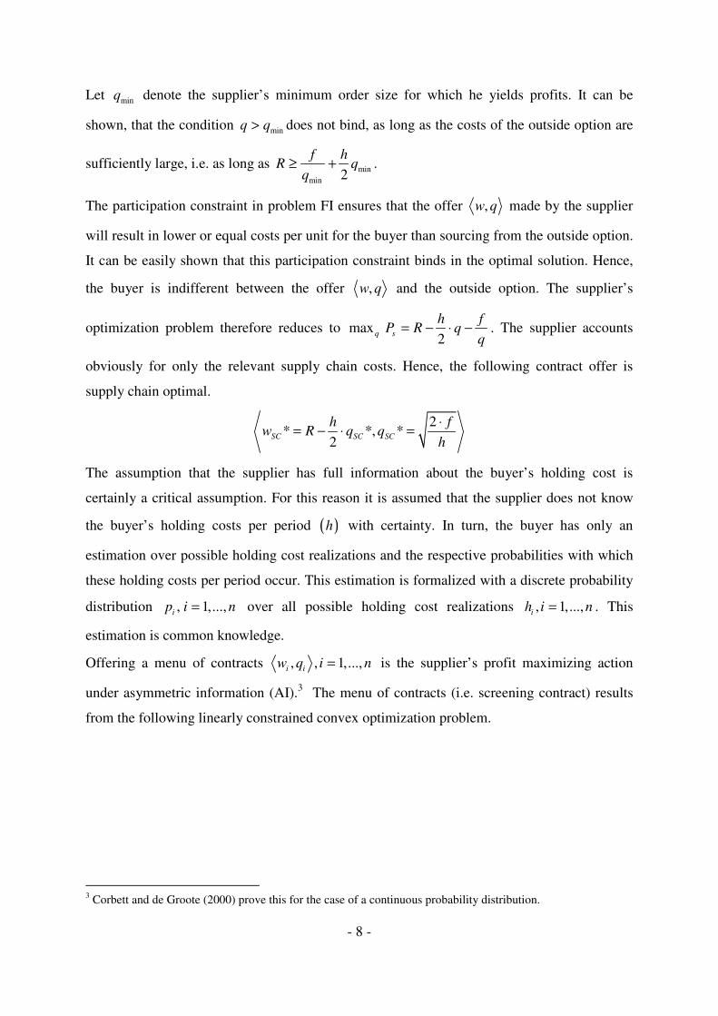
Problem FI:
,
min
max
. .
(participation constraint)2
q q
q w s
b
fP w
q
s t
hC w q R
= −
= + ⋅ ≤
≥
- 8 -
Let minq denote the supplier’s minimum order size for which he yields profits. It can be
shown, that the condition minq q> does not bind, as long as the costs of the outside option are
sufficiently large, i.e. as long as min
min 2
f hR q
q≥ + .
The participation constraint in problem FI ensures that the offer ,w q made by the supplier
will result in lower or equal costs per unit for the buyer than sourcing from the outside option.
It can be easily shown that this participation constraint binds in the optimal solution. Hence,
the buyer is indifferent between the offer ,w q and the outside option. The supplier’s
optimization problem therefore reduces to max2q s
h fP R q
q= − ⋅ − . The supplier accounts
obviously for only the relevant supply chain costs. Hence, the following contract offer is
supply chain optimal.
2* *, *
2SC SC SC
h fw R q q
h
⋅= − ⋅ =
The assumption that the supplier has full information about the buyer’s holding cost is
certainly a critical assumption. For this reason it is assumed that the supplier does not know
the buyer’s holding costs per period ( )h with certainty. In turn, the buyer has only an
estimation over possible holding cost realizations and the respective probabilities with which
these holding costs per period occur. This estimation is formalized with a discrete probability
distribution , 1,...,i
p i n= over all possible holding cost realizations , 1,...,i
h i n= . This
estimation is common knowledge.
Offering a menu of contracts , , 1,...,i iw q i n= is the supplier’s profit maximizing action
under asymmetric information (AI).3 The menu of contracts (i.e. screening contract) results
from the following linearly constrained convex optimization problem.
3 Corbett and de Groote (2000) prove this for the case of a continuous probability distribution.
- 9 -
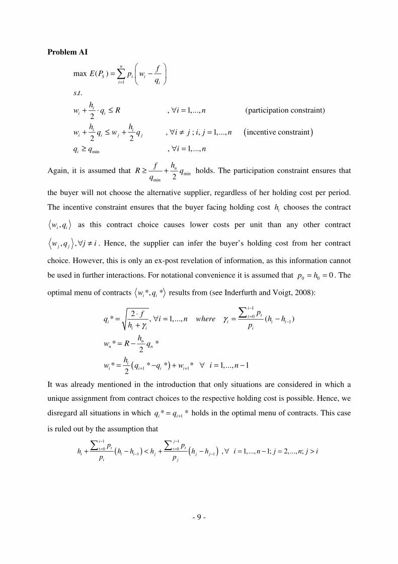
Problem AI
( )
1
min
max ( )
. .
, 1,..., (participation constraint)2
, ; , 1,..., incentive constraint2 2
, 1,...,
n
S i i
i i
i
i i
i i
i i j j
i
fE P p w
q
s t
hw q R i n
h hw q w q i j i j n
q q i n
=
= −
+ ⋅ ≤ ∀ =
+ ≤ + ∀ ≠ =
≥ ∀ =
∑
Again, it is assumed that min
min 2nhf
R qq
≥ + holds. The participation constraint ensures that
the buyer will not choose the alternative supplier, regardless of her holding cost per period.
The incentive constraint ensures that the buyer facing holding cost i
h chooses the contract
,i iw q as this contract choice causes lower costs per unit than any other contract
, ,j j
w q j i∀ ≠ . Hence, the supplier can infer the buyer’s holding cost from her contract
choice. However, this is only an ex-post revelation of information, as this information cannot
be used in further interactions. For notational convenience it is assumed that 0 0 0p h= = . The
optimal menu of contracts *, *i iw q results from (see Inderfurth and Voigt, 2008):
( )
1
01
1 1
2* , 1,..., ( )
* *2
* * * * 1,..., 12
i
tt
i i i i
i i i
n
n n
i
i i i i
pfq i n where h h
h p
hw R q
hw q q w i n
γγ
−
=−
+ +
⋅= ∀ = = −
+
= −
= − + ∀ = −
∑
It was already mentioned in the introduction that only situations are considered in which a
unique assignment from contract choices to the respective holding cost is possible. Hence, we
disregard all situations in which 1* *i i
q q += holds in the optimal menu of contracts. This case
is ruled out by the assumption that
( ) ( )1 1
0 01 1 , 1,..., 1; 2,..., ;
i j
t tt t
i i i j j j
i j
p ph h h h h h i n j n j i
p p
− −
= =− −+ − < + − ∀ = − = >
∑ ∑
- 10 -
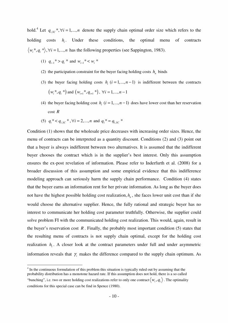
hold.4 Let , *, 1,...,i SC
q i n∀ = denote the supply chain optimal order size which refers to the
holding costs i
h . Under these conditions, the optimal menu of contracts
*, * , 1,...,i iw q i n∀ = has the following properties (see Sappington, 1983).
(1) 1* *i i
q q− > and 1* *i i
w w− <
(2) the participation constraint for the buyer facing holding costs n
h binds
(3) the buyer facing holding costs ( 1,..., 1)= −i
h i n is indifferent between the contracts
( )*, *i iw q and ( )1 1*, *i iw q+ + , 1,..., 1i n∀ = −
(4) the buyer facing holding cost ( 1,..., 1)= −i
h i n does have lower cost than her reservation
cost R
(5) ,* * , 2,...,i i SCq q i n< ∀ = and 1 1,* *SCq q=
Condition (1) shows that the wholesale price decreases with increasing order sizes. Hence, the
menu of contracts can be interpreted as a quantity discount. Conditions (2) and (3) point out
that a buyer is always indifferent between two alternatives. It is assumed that the indifferent
buyer chooses the contract which is in the supplier’s best interest. Only this assumption
ensures the ex-post revelation of information. Please refer to Inderfurth et al. (2008) for a
broader discussion of this assumption and some empirical evidence that this indifference
modeling approach can seriously harm the supply chain performance. Condition (4) states
that the buyer earns an information rent for her private information. As long as the buyer does
not have the highest possible holding cost realization,n
h , she faces lower unit cost than if she
would choose the alternative supplier. Hence, the fully rational and strategic buyer has no
interest to communicate her holding cost parameter truthfully. Otherwise, the supplier could
solve problem FI with the communicated holding cost realization. This would, again, result in
the buyer’s reservation cost R . Finally, the probably most important condition (5) states that
the resulting menu of contracts is not supply chain optimal, except for the holding cost
realization 1h . A closer look at the contract parameters under full and under asymmetric
information reveals that i
γ makes the difference compared to the supply chain optimum. As
4 In the continuous formulation of this problem this situation is typically ruled out by assuming that the probability distribution has a monotone hazard rate. If this assumption does not hold, there is a so called
“bunching”, i.e. two or more holding cost realizations refer to only one contract ,i iw q . The optimality
conditions for this special case can be find in Spence (1980).

- 11 -
0, 1,...,i
i nγ ≥ ∀ = , it is obvious that the order sizes are too low compared to the supply chain
optimum, i.e. there is a downward distortion of order sizes.5 Standard-theory predicts that this
coordination deficit (i.e. the performance deficit that results from a downward distortion of
order sizes) cannot be overcome as long as all supply chain members act individually rational
and opportunistic. Particularly, this expected coordination deficit, CD , can be expressed as
follows:
*,
1 ,
** 2 * 2
ni i
i i i SC
i i i SC
h hf fCD p q q
q q=
= + ⋅ − − ⋅
∑
The main objective of the underlying analysis, thus, is to investigate whether communication
and trust (as defined in section 2) can enhance supply chain performance or leads to a
deterioration of the overall supply chain performance.
4 The impact of communication and trust on supply chain
performance
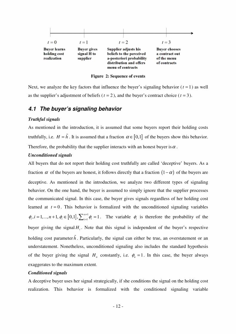
In the following it is assumed that the supplier receives a signal from the buyer before he
offers the menu of contract. The following sequence of events results: the buyer first learns
her holding cost [ ]1 ,..., nh h h∈ɶ . Then, the buyer communicates a holding cost to the supplier.
The buyer is restricted to signals H that are possible holding cost realizations or she can
refuse to give a signal, i.e. 1 1 1( ,..., ,..., , " ")+∈ = = = =i i n n n
H H h H h H h H No signal . Then,
the supplier decides to adjust the a-priori probabilities i
p to the perceived a-posteriori
probability distribution ( )ˆ ( | ) 1,..., ; 1,..., 1∀ = = +i i kp h H i n k n , which is conditioned on the
buyer’s signal. Then, the supplier calculates the menu of contracts with respect to the
perceived a-posteriori distribution and offers this screening contract to the buyer. Finally, the
buyer chooses one contract out of the menu of contracts. The following figure 2 depicts the
sequence of events.
5 It is referred to Inderfurth and Voigt (2008) for a broader discussion of the distortion caused by asymmetric information.
- 12 -
Figure 2: Sequence of events Next, we analyze the key factors that influence the buyer’s signaling behavior ( 1t = ) as well
as the supplier’s adjustment of beliefs ( 2t = ), and the buyer’s contract choice ( 3t = ).
4.1 The buyer’s signaling behavior
Truthful signals
As mentioned in the introduction, it is assumed that some buyers report their holding costs
truthfully, i.e. H h= ɶ . It is assumed that a fraction [ ]0,1α ∈ of the buyers show this behavior.
Therefore, the probability that the supplier interacts with an honest buyer isα .
Unconditioned signals
All buyers that do not report their holding cost truthfully are called ‘deceptive’ buyers. As a
fraction α of the buyers are honest, it follows directly that a fraction ( )1 α− of the buyers are
deceptive. As mentioned in the introduction, we analyze two different types of signaling
behavior. On the one hand, the buyer is assumed to simply ignore that the supplier processes
the communicated signal. In this case, the buyer gives signals regardless of her holding cost
learned at 0t = . This behavior is formalized with the unconditioned signaling variables
[ ]1
1, 1,..., 1, 0,1 , 1
n
i i iii nφ φ φ
+
== + ∈ =∑ . The variable
iφ is therefore the probability of the
buyer giving the signali
H . Note that this signal is independent of the buyer’s respective
holding cost parameter hɶ . Particularly, the signal can either be true, an overstatement or an
understatement. Nonetheless, unconditioned signaling also includes the standard hypothesis
of the buyer giving the signal n
H constantly, i.e. 1n
φ = . In this case, the buyer always
exaggerates to the maximum extent.
Conditioned signals
A deceptive buyer uses her signal strategically, if she conditions the signal on the holding cost
realization. This behavior is formalized with the conditioned signaling variable
- 13 -
[ ]( ), 1,..., 1, 1,..., , ( ) 0,1 .i k i kh i n k n hφ φ= + = ∈ A complete strategy profile requires that
1
1( ) 1, 1,...,
n
i kih k nφ
+
== ∀ =∑ holds. As an example, the buyer who always exaggerate her
holding cost by one (possible) unit and gives no signal if she faces the highest holding cost
realization has the strategy profile ( ) 1, 1, 1,...,i k
h i k k nφ = ∀ = + = and
( ) 0, 1, 1,...,i k
h i k k nφ = ∀ ≠ + = .
4.2 The supplier’s probability adjustment
The supplier is aware of the fact that there are some honest buyers. However, as there are also
deceptive buyers, he has to estimate the probability that he is interacting with an honest buyer.
This subjective probability is denoted by [ ]ˆ 0,1α ∈ . Furthermore, the supplier needs to
estimate the unconditioned signaling variables ˆ , 1,..., 1i
i nφ ∀ = + or the conditioned signaling
variables ˆ ( ), 1,..., 1; 1,...,i k
h i n k nφ ∀ = + = , respectively. It is assumed that the supplier can
observe whether the buyer conditions her signals or not.6 In the following we will only
present the supplier’s adjustment of beliefs in case of a buyer who gives unconditioned
signals. The analysis, however, can be easily transferred to the case where the buyer uses
conditioned signaling variables instead.
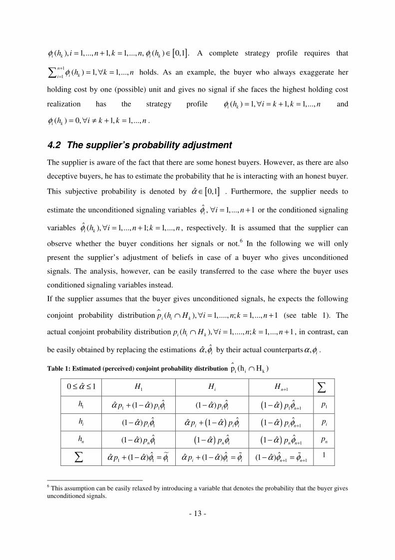
If the supplier assumes that the buyer gives unconditioned signals, he expects the following
conjoint probability distribution � ( ), 1,...., ; 1,..., 1i ki
p h H i n k n∩ ∀ = = + (see table 1). The
actual conjoint probability distribution ( ), 1,...., ; 1,..., 1i i k
p h H i n k n∩ ∀ = = + , in contrast, can
be easily obtained by replacing the estimations ˆˆ,i
α φ by their actual counterparts ,i
α φ .
Table 1: Estimated (perceived) conjoint probability distribution ɵ i kip (h H )∩
ˆ0 1α≤ ≤ 1H i
H 1nH + ∑
1h 1 1 1
ˆˆ ˆ(1 )+ −p pα α φ 1ˆˆ(1 )−i
pα φ ( ) 1 1ˆˆ1 +− npα φ 1p
ih
1ˆˆ(1 )−
ipα φ ( ) ˆˆ ˆ1+ −i i ip pα α φ ( ) 1
ˆˆ1 +− i npα φ ip
nh
1ˆˆ(1 )−
npα φ ( ) ˆˆ1− n ipα φ ( ) 1
ˆˆ1 +− n npα φ np
∑ �1 1 1
ˆˆ ˆ(1 )+ − =pα α φ φ ˆˆ ˆ(1 )+ − = ɶi i i
pα α φ φ 1 1ˆˆ(1 ) + +− = ɶn nα φ φ 1
6 This assumption can be easily relaxed by introducing a variable that denotes the probability that the buyer gives unconditioned signals.
- 14 -
Let � ( | ), 1,..., ; 1,...., 1i ki
p h H i n k n= = + denote the perceived a-posteriori probability that the
buyer giving signal k
H faces holding cost i
h . These perceived a-posteriori probabilities result
from:
ˆˆ ˆ(1 )ˆ ( | ) , 1,...,
ˆˆ(1 )ˆ ( | ) , 1,..., ; 1,..., 1;
i i i
i i i
i
i k
i i k
k
p pp h H i n
pp h H i n k n i k
α α φ
φ
α φ
φ
+ −= ∀ =
−= ∀ = = + ≠
ɶ
ɶ
This distribution is utilized to calculate the menu of contracts, i.e. the supplier solves the
problem AI with respect to � ( | ), 1,..., ; 1,...., 1i ki
p h H i n k n= = + . The resulting optimal
wholesale prices are denoted by k
iw and the respective order sizes are denoted by k
iq ,
1,...., ; 1,..., 1i n k n∀ = = + .
Throughout this study it is assumed that the supplier will always offer the ‘full’ menu of
contracts, i.e. he always offers n contracts which satisfy the incentive- and participation
constraint in problem AI. This ensures that the supplier offers the contract ,k k
i iw q even
though he adjusts his beliefs to � ( | ) 0i ki
p h H = . If this assumption does not hold, there might
be situations in which the buyer’s participation constraint is not satisfied.
The perceived probabilities determine the supplier’s contract offer ( 2t = ), whereas the actual
probabilities determine the relative frequency of the buyer’s contract choice ( 3t = ). Please
note that the notation is summarized in the appendix 9.2.
4.3 The buyer’s contract choice and the impact on the supplier
profits, the buyers cost and the overall supply chain deficit
The buyer’s expected contract choice ( 3t = ) is determined by the actual conjoint probability
distribution ( ), 1,...., ; 1,..., 1i i k
p h H i n k n∩ ∀ = = + . In the following we analyze the deviation
from the standard-theory’s predictions (i.e. without communication or trust). The main focus
of this analysis, thus, is to investigate whether communication enhances or deteriorates supply
chain performance compared to the game theoretic equilibrium without communication.

- 15 -
The expected change of the supplier’s profit, ( )SE P∆ , results from the profit difference
between the screening menu based on the perceived a-posteriori
distribution, , , 1,..., ; 1,..., 1k k
i iw q i n k n∀ = = + , and the screening menu based on the a-priori
distribution, *, * , 1,...,i iw q i n∀ = . All of these differences are weighted by the respective
actual conjoint probability distribution, i.e. these cost differences are weighted by the
probability that a buyer faces holding cost i
h while signalingk
H . Hence, the expected change
of the supplier’s expected profit results from:
( ) ( )1
, ,1 1
**
n nk k k
S i i k s i s i i iki k ii
f fE P p h H P where P w w
+
= =
∆ = ∩ ∆ ⋅ ∆ = − − +∑∑
The same calculation can be done for the buyer with respect to her cost function. Then, the
expected difference of the honest buyer’s expected costs results from
( ),1
* *2 2
ni ii i
b honest i i i i i
i
h hE C p w q w qα
=
∆ = + − −
∑ ,
and the expected difference of the deceptive buyer’s expected costs results from
( ) ( ),1 1
1 * *2 2
n nk ki i
b deceptive i k i i i i
k i
h hE C p w q w qα φ
= =
∆ = − + − −
∑∑ .
Hence, the total expected difference of the honest as well as the deceptive buyer’s expected
costs results from:
( ) ( ) ( )1
, , ,1 1
,
( )
* *.2 2
n nk
b b honest b deceptive i i k b i
i k
k k ki i
b i i i i i
E C E C E C p h H C
h hwhere C w q w q
+
= =
∆ = ∆ + ∆ = ∩ ∆ ⋅
∆ = + − −
∑∑
Finally, the expected change of the supply chain performance results from:
( ) ( )
( ) ( )
1
1 1
( )
*
( )2
n nk
b S i i k i
i k
k k
i SC i SC i
k ki
SC i ik
i
CD E C E P p h H CD
where
CD C q C q
hfC q q
q
+
= =
∆ = ∆ − ∆ = ∩ ∆ ⋅
∆ = −
= +
∑∑
( ) ( )*k k
i SC i SC iCD C q C q∆ = − denotes the supply chain cost differences that arise due to the
adjustment of the a-priori probabilities. For 0CD∆ ≤ the supply chain deficit decreases due to

- 16 -
communication, which is identical to an improvement of the overall supply chain
performance. In this case, communication is an appropriate coordination mechanism.
Otherwise, it is not.
5 Impact of communication in case of unconditioned
signals
5.1 General analysis
If the buyer believes that the supplier ignores the signal, she is assumed to use unconditioned
signals. In this case the following general predictions regarding the supplier’s expected
profits, the buyer’s expected costs and the supply chain’s deficit can be derived. All proofs
can be find in the appendix 9.1.
Theorem 1: The supplier’s expected profits do not decrease due to the adjustment of the a-
priori distribution as long as ii
i i i
ˆˆ min , i 1,..., n
ˆ
φ ⋅ αα ≤ =
φ ⋅ α + φ − φ α holds.
Theorem 1 shows that the supplier should be cautious to believe too much in the buyer’s
signal. This means, that he should rather underestimate the number of buyers who are honest
than to overestimate this number. Yet, on the other hand the supplier cannot participate from
truthful signals if he chooses α̂ too low because the probability adjustment is not rigorously
enough. As an example, the supplier will not adjust his probabilities at all if ˆ 0α = holds
although all buyers are honest, i.e. 1α = . In this case communication has no effect, simply
because the supplier does not react to the signals.
Note that the condition in theorem 1 is always satisfied if α̂ α≤ and ˆ , 1,..., 1i i
i nφ φ= = +
holds. Thus, if the supplier can perfectly observe the buyer’s unconditioned signals, and if his
estimation with respect to the buyer’s trustworthiness is equal or lower than the buyer’s actual
trustworthiness, the supplier will always gain from communication. The increase of expected
profits for the above parameter combinations can be explained by the finding, that for these
parameters the supplier is always closer to the actual a-posteriori distribution than if he would
stick to the a-priori distribution, i.e. ˆ ( | ) ( | )i i i i i i i
p p h H p h H≤ ≤ and
ˆ( | ) ( | ) ,i i k i i k i
p h H p h H p i k≤ ≤ ∀ ≠ hold. In fact, if ( ) ( )ˆ ˆˆ /i i i i
α φ α φ α φ φ α= ⋅ ⋅ + − holds

- 17 -
for a specific signal i
H , then the supplier estimates the actual a-posteriori distribution with
respect to the signal i
H accurately whereas the accuracy decreases with decreasing α̂ .
If the above condition is not satisfied the supplier’s expected profits can increase nonetheless.
In this case he overestimates the probability which corresponds to the respective signal, i.e.
ˆ( | ) ( | )i i i i i i i
p p h H p h H≤ ≤ , and underestimates all other probabilities, i.e.
ˆ ( | ) ( | ) ,i i k i i k i
p h H p h H p i k≤ ≤ ∀ ≠ . In this case, the change in the supplier’s expected
profits is dependent on the specific parameter values.
Theorem 2.1: The honest buyer’s expected costs increase due to truthful signaling.
The supplier will decrease all order sizes that corresponds to the holding costs that are higher
than the signal, i.e. *,k
i iq q i k≤ ∀ > given signal
kH . The expected cost, thus, will increase
due to the ‘indifference’-condition (3) (see chapter 3).
Theorem 2.2: The expected costs of the deceptive buyer can either increase or decrease due
to communication.
The deceptive buyer can be worse off due to communication, if she reports (accidentally)
truthful or if she understates her actual holding costs. The argumentation is equal to theorem
2.1. If the deceptive buyer exaggerates her holding cost constantly to the maximum extent
(i.e. 1n
φ = ), however, then she cannot be worse off due to communication. If the deceptive
buyer exaggerates not to the maximum extent, though, her expected costs changes are
dependent on the specific parameters values.
Theorem 3.1: The supply chain optimum is achieved if ˆ 1α α= = holds. The supply chain
performance is worst if 1ˆ1, 0 1andφ α α= = = holds.
For ˆ 1α α= = the supply chain faces a decision problem as if under full information. This
results in the supply chain optimum.
For 1ˆ1, 0 1andφ α α= = = it follows, that all buyers are deceptive and constantly claim that
they have the lowest possible holding costs. The supplier will, in turn, decrease all order sizes
1 *, 2,...,i i
q q i n≤ ∀ = . As the order size 1 1*, 1,..., 1kq q k n= ∀ = + does not change due to an
adjustment of the probabilities (see section 3, condition (5)) the downward distortion increases
for all order sizes.

- 18 -
Theorem 3.2: As long as ( )
( ),
,
ˆˆ,1
k i
i k i i i i
i k i k i
crit ik i
i k i i i i
i k i k i
p CD p CD
p CD p CD
φ φ
α α α φφ φ
≠
≠
∆ + ∆
≥ =∆ − − ∆
∑∑ ∑
∑∑ ∑ holds,
communication enhances the supply chain performance.
This theorem points out that there are regions of parameter values in which communication
improves supply chain performance, but that there are also parameters values for which the
supply chain performance deteriorates. Intuitively, communication becomes more attractive
from a supply chain perspective the higher the fraction of honest buyers, α . However, as
soon as this fraction α decreases under the critical level ( )ˆˆ,crit i
α α φ , the more likely are
situations in which a deceptive buyer unconditionally misrepresents her holding cost
realization while the supplier reacts to this signal. From ( )ˆˆ, 1crit i
α α φ ≤ it follows directly that
communication can always be an appropriate coordination mechanism as long as the number
of honest buyers is sufficiently large.
Theorem 3.3: Given a certain probability that the supplier interacts with an honest buyer, i.e.
α , it is more likely that communication is an appropriate coordination mechanism if the
supplier’s trust in the buyer’s signal decrease, i.e. if α̂ decrease.
This theorem gives an interesting insight into the interaction between trust (α̂ ) and
trustworthiness (α ) and the impact of this interaction on supply chain performance.
Particularly, this theorem shows that more trust does not necessarily increase the supply chain
performance. In contrary, the more the supplier trusts the buyer’s signal, the more likely is a
deterioration of supply performance. The effectiveness of communication decreases on the
other hand, if the supplier’s trust decreases because he simply does not adjust the probabilities
rigorously enough. Hence, it is an important challenge of supply chain management to
identify an appropriate level of trust.
5.2 Numerical Example
In the following the previous analysis for the case of two possible holding cost realizations,
i.e. [ ]1 2,h h h∈ , is illustrated. Suppose that ( ) ( )1 2 3 1 2 3ˆ ˆ ˆ, , , ,= =φ φ φ φ φ φ ( )1 1 1; ;3 3 3 ,
( ) ( )1 21 1; ;2 2=p p , ( )1 2( ; ) 1;2=h h , 801=R , ˆ 0.5=α , 0.6=α , min 1q = and 800f = .
- 19 -
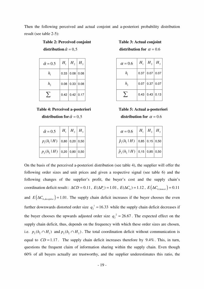
Then the following perceived and actual conjoint and a-posteriori probability distribution
result (see table 2-5):
Table 2: Perceived conjoint Table 3: Actual conjoint
distribution ˆ 0,5=α distribution for 0.6=α
Table 4: Perceived a-posteriori Table 5: Actual a-posteriori
distribution for ˆ 0,5=α distribution for 0.6=α
On the basis of the perceived a-posteriori distribution (see table 4), the supplier will offer the
following order sizes and unit prices and given a respective signal (see table 6) and the
following changes of the supplier’s profit, the buyer’s cost and the supply chain’s
coordination deficit result:: 0.11CD∆ = , ( ) 1.01∆ =s
E P , ( ) 1.12∆ =b
E C , ( ), 0.11b honest
E C∆ =
and ( ), 1.01b deceptive
E C∆ = . The supply chain deficit increases if the buyer chooses the even
further downwards distorted order size 12 16.33q = while the supply chain deficit decreases if
the buyer chooses the upwards adjusted order size 22 26.67q = . The expected effect on the
supply chain deficit, thus, depends on the frequency with which these order sizes are chosen,
i.e. 2 2 1( )p h H∩ and 2 2 2( )p h H∩ . The total coordination deficit without communication is
equal to 1.17CD = . The supply chain deficit increases therefore by 9.4% . This, in turn,
questions the frequent claim of information sharing within the supply chain. Even though
60% of all buyers actually are trustworthy, and the supplier underestimates this ratio, the
ˆ 0.5α = 1H 2H 3H
1h 0.33 0.08 0.08
2h 0.08 0.33 0.08
∑ 0.42 0.42 0.17
0.6α = 1H 2H 3H
1h 0.37 0.07 0.07
2h 0.07 0.37 0.07
∑ 0.43 0.43 0.13
0.6α = 1H 2H 3H
1 1ˆ ( | )p h H 0,85 0,15 0,50
2 2ˆ ( | )p h H 0,15 0,85 0,50
ˆ 0.5α = 1H 2H 3H
1 1( | )p h H 0,80 0,20 0,50
2 2( | )p h H 0,20 0,80 0,50
- 20 -
supply chain deficit increases. In fact, the supply chain deficit would only decrease due to
communication if 0.67crit
α α> = holds (see theorem 3.2).
Table 6: Order sizes and unit prices in the menu of contracts
Signal
a-priori supply chain
Optimum a-posteriori 1H 2H 3H
1 *q 40 1, *SC
q 40 1k
q 40 40 40
2 *q 23.09 2, *SC
q 28.28 2k
q 16.33 26.67 23.09
1 *w 769.45 - - 1k
w
772.84 767.67 769.45
2 *w 777.91 - - 2k
w
784.67 774.33 777.91
The supplier’s expected profits increase due to communication, which is in line with theorem
1 (as the condition in theorem 1 holds). The buyer, in turn, is worse off, independent of
whether she is honest or deceptive. This stresses that unconditioned signals can substantially
deteriorate the performance even of the deceptive buyer (see theorem 2.2).
Yet, the previous analysis showed that the effect of communication on supply chain
performance is ambiguous. An example in which communication is effective can be easily
constructed by settingcrit
α α> . In this case, it is more likely that the performance improving
order size 22q instead of the performance deteriorating order size 1
2q is chosen (see Table 6).
To test the impact of the several parameters and variables a comparative static analysis is
conducted in the next section.
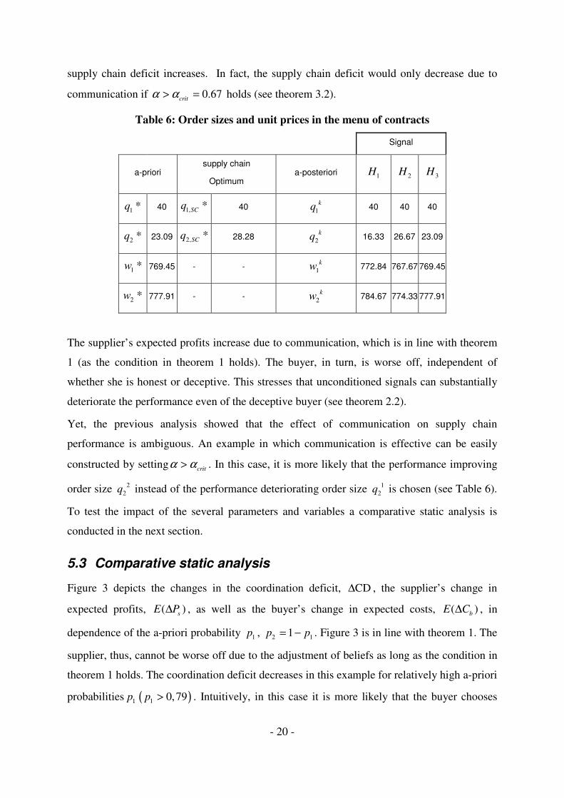
5.3 Comparative static analysis
Figure 3 depicts the changes in the coordination deficit, CD∆ , the supplier’s change in
expected profits, ( )∆ sE P , as well as the buyer’s change in expected costs, ( )∆ bE C , in
dependence of the a-priori probability 1p , 2 11p p= − . Figure 3 is in line with theorem 1. The
supplier, thus, cannot be worse off due to the adjustment of beliefs as long as the condition in
theorem 1 holds. The coordination deficit decreases in this example for relatively high a-priori
probabilities 1p ( )1 0,79p > . Intuitively, in this case it is more likely that the buyer chooses
- 21 -
the undistorted order size 11q instead of the distorted order size 1
2q . Furthermore, from
2
2 2
2*
fq
h γ
⋅=
+ and 1
2 2 1
2
( )p
h hp
γ = − (see Section 3) it follows directly that there is a
comparably stronger adjustment of the order size 2 , 1,2,3kq k = if the a-priori probability 2p
is low, because 22
2 2
1
p p
γ∂= −
∂ holds. As coordination potentials are only used through an
upward adjustment of 22q , the coordination deficit decreases for low values 2p or high values
1p respectively (see Section 3, condition (5)). As an example, the supplier adjusts the order
sizes from 2* 12.06q = to 12 7.11q = and 2
2 18.38q = when 1 0.9p = holds.
Additionally, figure 3 shows that the supply chain performance does not automatically
increase if the supplier’s estimation of the a-posteriori distribution is more accurate (which is
always the case if the condition in theorem 1 holds). As the supplier maximizes his own
expected profits instead of minimizing the overall expected supply chain costs, the supply
chain deficit can increase even if the supplier estimates the buyer’s holding costs more
accurately through communication.
Figure 3: Variation of the a-priori probability 1p
- 22 -
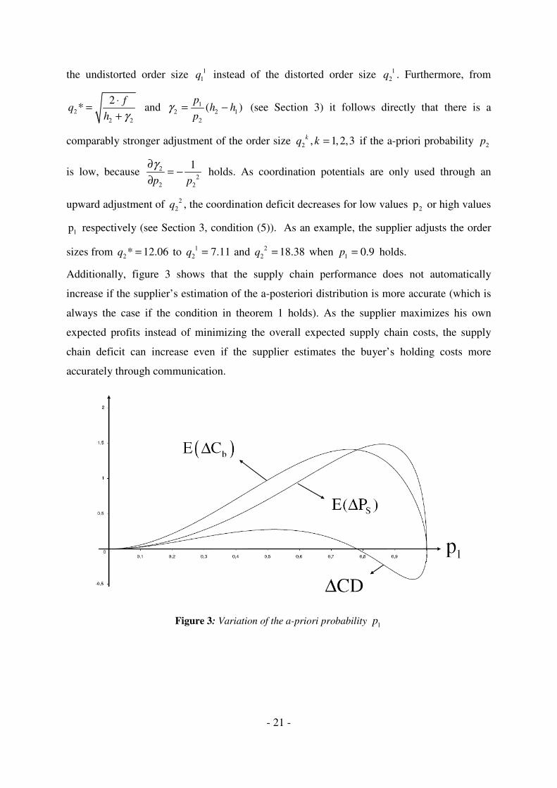
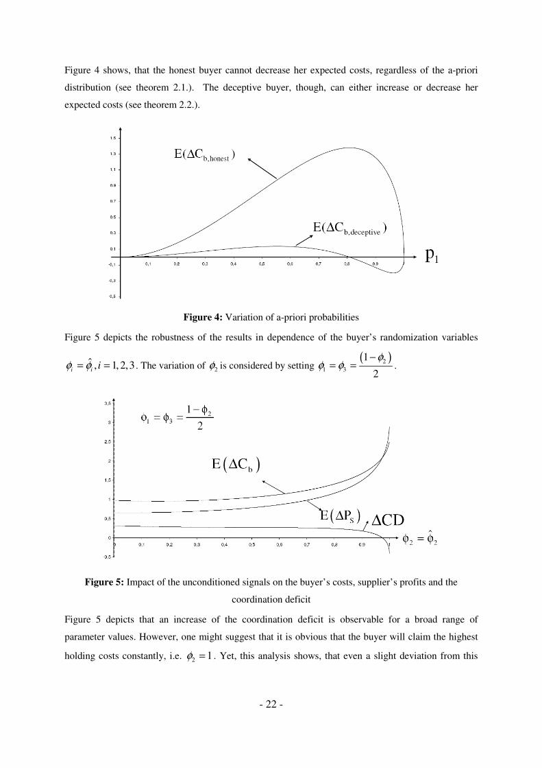
Figure 4 shows, that the honest buyer cannot decrease her expected costs, regardless of the a-priori
distribution (see theorem 2.1.). The deceptive buyer, though, can either increase or decrease her
expected costs (see theorem 2.2.).
Figure 4: Variation of a-priori probabilities
Figure 5 depicts the robustness of the results in dependence of the buyer’s randomization variables
ˆ , 1, 2,3i i
iφ φ= = . The variation of 2φ is considered by setting ( )2
1 3
1
2
φφ φ
−= = .
Figure 5: Impact of the unconditioned signals on the buyer’s costs, supplier’s profits and the
coordination deficit
Figure 5 depicts that an increase of the coordination deficit is observable for a broad range of
parameter values. However, one might suggest that it is obvious that the buyer will claim the highest
holding costs constantly, i.e. 2 1φ = . Yet, this analysis shows, that even a slight deviation from this

- 23 -
behavior ( 2 0,97φ < ), as observed by Inderfurth et al. (2008), can harm the overall supply chain
performance.
Figure 6: Impact of unconditional signals on the honest and deceptive buyer’s expected costs.
Figure 6 again stresses that the rationally deceptive buyer would choose the unconditional signal
2 1φ = if she assumes that the supplier updates his beliefs with respect to the signal. An honest buyer,
however, benefits from a deviating behavior, as the increase in expected costs is lower for lower
values of 2 2ˆφ φ= . This effect is prevalent, because in this case it is harder for the supplier to
distinguish whether signal 1H was given by a honest or by a dishonest buyer.
In the following, we investigate the impact of the supplier’s trust as well as the buyer’s
trustworthiness. For this purpose, the level of the supplier’s trust is fixed at ˆ 0,5α = (as in the
numerical example) while the buyer’s trustworthiness, α , varies. Figure 7 shows that the expected
profits of the supplier can decrease, if the overestimation of the buyer’s trustworthiness is relatively
high (see theorem 1). In the numerical example the suppliers expected profits would decrease for
0, 27α < . In turn, the coordination deficit decreases for 0,67crit
α > .7 Figure 8 depicts the critical
levels of trustworthiness, crit
α , in dependence of the supplier’s trust, α , for which the supply chain
performance does not change compared to the benchmark without communication. Furthermore, the
arrows depicts in which regions the supply chain deficit would increase and decrease. These regions
directly follow from theorem 3.3.
7 Surprisingly, if it is assumed that the supplier can perfectly observe the buyers trustworthiness, i.e. ˆα = α ,
then the coordination deficit would only decrease for ˆ 0.98α = α > .

- 24 -
Figure 7: Variation α
Figure 8 shows that communication becomes less attractive from a coordinational point of view, the
higher the supplier’s trust in the buyers signals, because crit
α is monotonically increasing with
increasing α . This counterintuitive result highlights that the unilateral claim for more trust in
supplier-buyer relationships might not always be justifiable. However, note that Figure 8 does not
depict the size of the changes in the coordination deficit. Obviously, if the supplier totally mistrust the
buyers signals, i.e. ˆ 0α = , then communication would have no impact on supply chain coordination
and 0crit
α = would hold. In this case, though, neither the supplier nor the supply chain could benefit
from trustworthy signals. The same analysis could be conducted for changes of i
φ . However, it can be
shown that a variation of α and i
φ have a similar impact on the supply chain performance. Hence,
this analysis is omitted.
Figure 8: Critical level of trustworthiness ( )critα in dependence of trust ( )α̂
- 25 -
6 Impact of communication in case of conditioned signals
The previous analysis concentrated on unconditioned signals, i.e. the buyer who chooses her
signal independently from her actual holding cost realization. Now, it is assumed that the
buyer conditions her signals on the actual holding cost realization. Therefore, conditioned
signaling variables, ( ) , ,i k
h i kφ ∀ are defined. These variables denote the probability that the
deceptive buyer facing holding cost k
h gives the signali
H . The deceptive buyer might, for
example, exaggerate her holding cost to the maximum extent, i.e. ( ) 1 1,...,n i
h i nφ = ∀ = .
Alternatively, she might always exaggerate her actual holding cost realization by one
(possible) unit, i.e. ( ) 1 1i k
h i kφ = ∀ = + .
Please note, that the buyer might convey information if she uses strategic signaling variables
and the supplier correctly anticipates this behavior. If the buyer always exaggerates by one
unit, and the supplier anticipates this correctly, the supplier could infer the holding cost from
the signal. In this case, the supplier has actually full information, which in turn leaves no
information rent to the deceptive buyer.
Again, it is assumed that the supplier estimates the buyer’s conditioned signaling variables.
This estimation is denoted by ɵ ( )i khφ .
The conditioned signaling variables are obviously a generalization of the assumption that the
buyer gives unconditioned signals. Particularly, if ( )i i k
hφ φ= and ˆ ˆ ( ), 1,...,i i k
h k nφ φ= ∀ =
holds, the same results apply. Hence, it is not surprising that the analysis becomes more
complex. Especially the previous theorems cannot be easily transferred. For this reason a
numerical example combined with a comparative static analysis demonstrates the differences
that emerge in contrast to the previous section, i.e. in contrast to unconditioned signals.
6.1 Numerical example and comparative static analysis
As a starting point, it is assumed that the supplier can perfectly observe the buyer’s
conditioned signaling variables. As an example, it is assumed that
1 1 1 1ˆ( ) ( ) 0h hφ φ= = 2 1 2 1
ˆ, ( ) ( ) 1h hφ φ= = , 3 1 3 1ˆ( ) ( ) 0h hφ φ= = , 1 2 1 2
ˆ( ) ( ) 1/ 3h hφ φ= = ,
2 2 2 2ˆ( ) ( ) 1/ 3h hφ φ= = and 3 2 3 2
ˆ( ) ( ) 1/ 3h hφ φ= = . All remaining parameter values from Section
5 apply. The buyer, thus, follows the strategy to always exaggerate her holding cost to the
maximum extent (i.e. by one unit) if she faces holding costs 1h . Yet, if she faces the holding
- 26 -
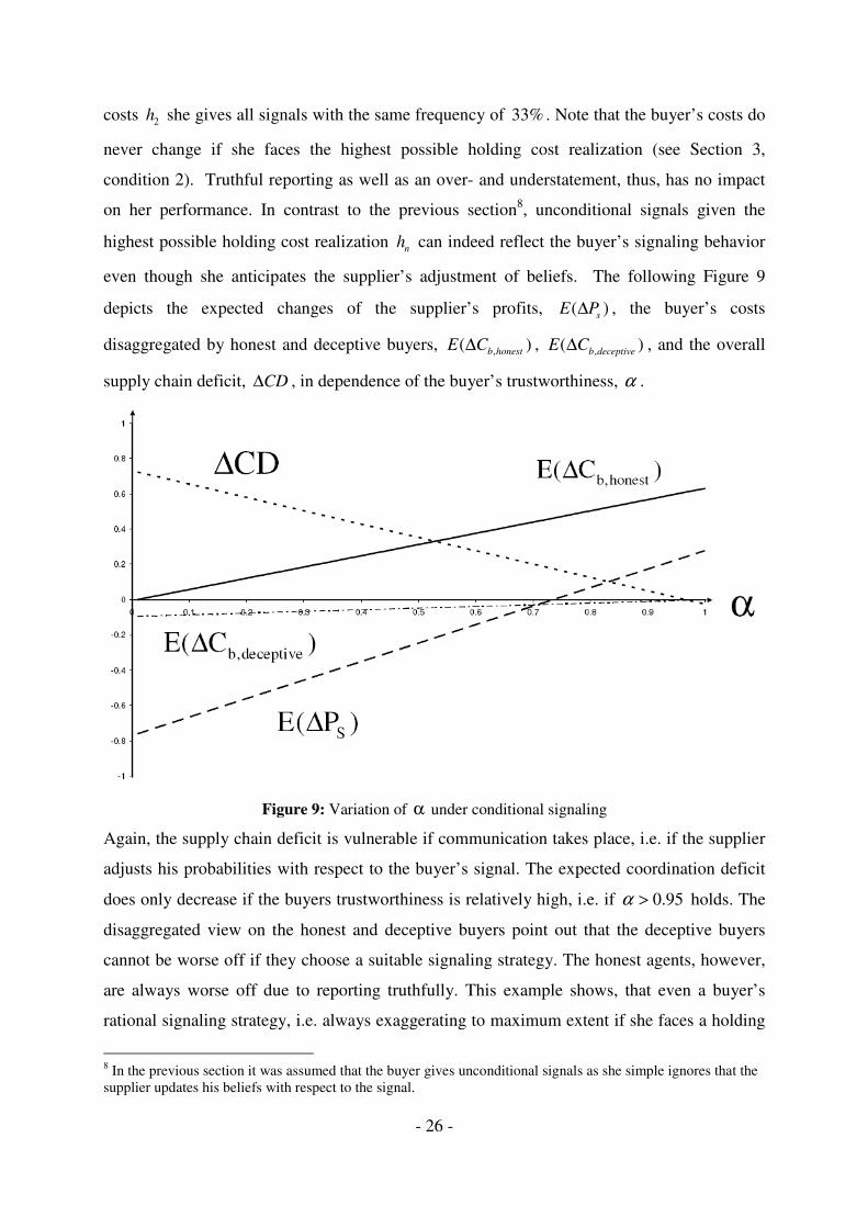
costs 2h she gives all signals with the same frequency of 33% . Note that the buyer’s costs do
never change if she faces the highest possible holding cost realization (see Section 3,
condition 2). Truthful reporting as well as an over- and understatement, thus, has no impact
on her performance. In contrast to the previous section8, unconditional signals given the
highest possible holding cost realization n
h can indeed reflect the buyer’s signaling behavior
even though she anticipates the supplier’s adjustment of beliefs. The following Figure 9
depicts the expected changes of the supplier’s profits, ( )s
E P∆ , the buyer’s costs
disaggregated by honest and deceptive buyers, ,( )b honest
E C∆ , ,( )b deceptive
E C∆ , and the overall
supply chain deficit, CD∆ , in dependence of the buyer’s trustworthiness, α .
Figure 9: Variation of α under conditional signaling
Again, the supply chain deficit is vulnerable if communication takes place, i.e. if the supplier
adjusts his probabilities with respect to the buyer’s signal. The expected coordination deficit
does only decrease if the buyers trustworthiness is relatively high, i.e. if 0.95α > holds. The
disaggregated view on the honest and deceptive buyers point out that the deceptive buyers
cannot be worse off if they choose a suitable signaling strategy. The honest agents, however,
are always worse off due to reporting truthfully. This example shows, that even a buyer’s
rational signaling strategy, i.e. always exaggerating to maximum extent if she faces a holding
8 In the previous section it was assumed that the buyer gives unconditional signals as she simple ignores that the supplier updates his beliefs with respect to the signal.

- 27 -
cost realization that is lower than n
h , while giving unconditional signals if she faces the
holding cost realization n
h , can significantly harm the overall supply chain performance. To
highlight the impact of the buyer’s unconditional signaling while facing the holding cost
realizationn
h , the buyers signaling strategy given n
h is varied. Figure 10 captures the changes
of the respective expected cost and profit changes for a change of 2 2( )hφ . The variation of
2 2( )hφ is considered by setting 3 2( ) 0hφ = and 1 2 2 2( ) 1 ( )h hφ φ= − . Furthermore, it is assumed
that the supplier expects that the buyer always exaggerate to the maximum extent, i.e.
2 1 2 2ˆ ˆ( ) ( ) 1h hφ φ= = . All other values from the previous example apply.
Figure 10: Variation of the conditional signaling strategy
This analysis points out that the supply chain performance is heavily dependent on the
supplier’s perception of the buyer’s signaling strategy and the signaling strategy itself. As an
example, for 2 2( ) 0.2hφ = the supply chain deficit increases by 148CD∆ = , i.e. the
coordination deficit is about 126 times higher than without communication. In contrary, the
buyer’s expected costs do not change (see Section 3, condition 2). The supplier, thus, should
carefully estimate the buyer’s unconditioned signaling variables. However, if this is not
possible he should be cautious to adjust the a-priori probabilities at all.
- 28 -
7 Managerial Insights & Conclusion
There is a growing body of work that analyses the inefficiencies of supply chain interactions
under asymmetric information in traditional principal-agent settings. Traditionally, it is
assumed that the principal has an a-priori probability distribution over the agent’s private
information. However, there is usually little said on how the principal obtains this
distribution. Moreover, it is stressed that the assessment of the a-priori distribution is not
influenced by communication, as information sharing is simply treated as cheap talk.
This study shows that the introduction of communication in the presence of trust and
trustworthiness can substantially affect the predictions of principal-agent models under
asymmetric information. The behavioral model introduced in this study therefore provides a
general framework which allows to investigate the impact of different information processing
and information sharing behavior in a general principal-agent framework.
In a typical supply chain lotsizing setup, it is shown that buyers have an incentive to
misrepresent their order size related costs. However, previous empirical work in the field of
supply chain coordination shows that not all buyers exploit their superior information. In fact,
there is a substantial level of honesty in supply chain interactions.
The underlying work shows that the effect of information processing on the supplier’s
performance is ambiguous. Particularly, if the supplier manages to assess the buyer’s
information sharing behavior accurately while underestimating the probability of receiving
credible signals, the supplier can indeed improve his performance. However, if the supplier
does not anticipate the buyer’s information sharing behavior accurately while being
overconfident in receiving credible information, a decrease in the supplier’s performance
level is likely.
Surprisingly, the results show that the overall supply chain performance can seriously
deteriorate, even though the supplier can utilize the shared information to assess a more
accurate estimation of the buyer’s private information. This fact stresses the basic conflict in
supply chain management, i.e. the supplier’s optimization attempts do not automatically lead
to supply chain optimal solutions. Therefore, communication can not be regarded as an
appropriate coordination instrument without considering the specific supply chain
environment. Managers should carefully evaluate whether their respective supply chain is
more likely to gain or to loose from information sharing. Hence, the ever increasing unilateral
claim for trust in supplier-buyer relationships does not seem to be appropriate.

- 29 -
The behavioral model introduced in the underlying work is subject to some limitations. First,
it is assumed that communication, trust and trustworthiness are exogenously determined. Yet,
another approach might treat these variables endogenously by incorporating reputational
effects in recurring interactions.
A further direction for research might be the extensive testing of this behavioral model
according to Inderfurth et al. (2008). This research might give valuable empirical data which
allows for an estimation of the behavioral parameters of the model.
8 References
Alger, I.; Renault, R. (2007): Screening ethics when honest agents keep their word,
in: Economic Theory 30, 291-311
Alger, I.; Renault, R. (2006): Screening ethics when honest agents care about fairness
in: International Economic Review 47 (1) , 59-85
Anderson, J.; Narus, J. (1984): A model of the distributor’s perspective of distributor-manufacturer
working relationships
in: Journal of Marketing 48(Fall), 62-74
Ben-Ner, A.; Putterman, L. (2001): Trusting and trustworthiness
in: Boston University Law Review 81(3), 523-551
Cachon, G. (2003): Supply chain coordination with contracts
in: Handbooks in Operations Research and Management Science: Supply Chain Management, edited
by Steve Graves and Ton de Kok, North-Holland, Amsterdam, The Netherlands, 229-257
Cachon, G.P.; Fisher, M. (2000): Supply Chain Inventory Management and the Value of Shared
Information
in: Management Science 46 (8), 1032-1048
Castaldo, S. (2007): Trust in market Relationships, Edward Elgar Publishing Ltd, Cheltenham.
Chen, F. (2003): Information sharing and supply chain coordination
in: Handbooks in Operations Research and Management Science: Supply Chain Management, edited
by Steve Graves and Ton de Kok, North-Holland, Amsterdam, The Netherlands, 341-413
Corbett, C.J. (2001): Stochastic inventory systems in a supply chain with asymmetric information:
Cycle stocks, safety stocks, and consignement stock
in: Management Science 49 (4), 487-500
- 30 -
Corbett, C.J.; de Groote, X. (2000): A supplier`s optimal quantity discount policy under asymmetric
information
in: Management Science 46 (3), 444-450
Corbett, C.J.; Tang, C.S. (2003): Designing supply contracts: Contract type and information
asymmetry
in: Quantitative Models for Supply Chain Management, edited by R. Ganeshan, S. Tayur and
M. Magazine, Kluwer Academic Publishers
Corbett, C.J.; Zhou, D.; Tang, C.S. (2004): Designing supply contracts: Contract type and
information asymmetry
in: Management Science 50 (4), 550-559
Crawford, V. (1998): A survey of experiments on communication via cheap talk
in: Journal of Economic Theory 78(3), 286-298
Eckel, C.C.; Wilson, R. K. (2004): Is trust a risky decision?
in: Journal of Economic Behavior & Organization 55, 447-465
Gambetta, D. (1988): Can we trust?
in: Making and breaking cooperative relations, edited by Diego Gambetta, Basil Blackwell, Oxford,
275-309
Ha, A.Y. (2000): Supplier-buyer contracting: Asymmetric cost information and cutoff level policy for
buyer participation
in: Naval Research Logistics 48(1), 41-64
Inderfurth, K.;Voigt, G. (2008): Setup cost reduction and supply chain coordination in case of
asymmetric information
in: FEMM Working Paper No. 16/2008,
http://www.uni-magdeburg.de/bwl6/download/2008_02_FEMM.pdf
Inderfurth, K.; Sadrieh, A., Voigt, G. (2008): The impact of cheap talk in case of asymmetric
information: An experimental Investigation
in: FEMM Working Paper No. 01/2008,
http://www.uni-magdeburg.de/bwl6/download/2008_01_FEMM.pdf
Kelle, P.; Akbulut, A. (2005): The role of ERP tools in supply chain information, cooperation, and
cost optimization
in: International Journal of Production Economics 93-94, 41-52
Mayer, R.C.; Davis, H.D.; Schoorman, F.D. (1995): An integrative model of organizational trust
in: The Academy of Management Review 20(3), 709-734

- 31 -
Minkler, L.P. und Miceli, T.J. (2004): Lying, Integrity, and Cooperation
in: Review of Social Economy 62(1), 27-50
Mohr, J.; Spekman, R. (1994): Characteristics of partnership success: partnership attributes,
communication behavior, and conflict resolution techniques
in: Strategic Management Journal 15(2), 135-152
Moore, K. R. (1998): Trust and relationship commitment in logistics alliances: a buyer perspective
in: International Journal of Purchasing and Materials Management 34(1), 24-37
Morgan, R.M.; Hunt, S.D. (1994): The commitment-trust theory of relationship marketing
in: Journal of Marketing 58(3), 20-38
Mui, M.M.; Halberstadt, A. (2002): A computational model of trust and reputation
in: Proceedings of the 35th Hawaii International Conference on System Sciences
Myerson, R.B. (1986): Multistage games with communication
in: Econometrica 54(2), 323-358
Özer, Ö.; Zheng, Y.; Chen, K.Y. (2008): Trust in forecast information sharing
Working Paper
Sako M. and Helper, S. (1998): Determinants of trust in supplier relations: evidence from the
automotive industry in Japan and the United States
in: Journal of Economic Behavior & Organization 34, 387-417
Sappington, D. (1983): Limited liability contracts between principal and agent.
in: Journal of Economic Theory 29, S.1-21
Schonberger, R.J.; Schniederjans, M.J. (1984): Reinventing inventory control
in: Interfaces 14(3), 76-83
Severinov, S.; Deneckere, R. (2006): Screening when some agents are non-strategic: Does a
monopoly need to exclude?
in : RAND Journal of Economics 37(4), S. 816-840
Sucky, E. (2006): A bargaining model with asymmetric information for a single supplier-single buyer
problem
in: European Journal of Operational Research 171, 516-535
Zaheer, A.; McEvily, B.; Perrone, V. (1998): The strategic value of buyer-supplier
relationships
in: International Journal of Purchasing and Materials Management 34(3), 20-26
Zand, D.E. (1972): Trust and managerial problem solving
in: Administrative Science Quarterly 17, 229-239
- 32 -
9 Appendix
9.1 Proofs of theorems
Theorem 1: The suppliers expected profits do not decrease due to the adjustment of the a-
priori distribution as long as ˆ
ˆ min , 1,...,ˆ
i
i
i i i
i nφ α
αφ α φ φ α
⋅≤ =
⋅ + − holds.
Proof:
In the following it is shown that the supplier estimates the actual a-posteriori distribution ( | )i i i
p h H
more accurately if the condition in theorem 1 holds.
a.) Adjustment of the probability that corresponds to the signal: ˆ ( | ), 1,...,∀ =i i i
p h H i n
First, it is shown that the perceived a-posteriori probability is always lower than the actual a-posteriori
probability if ˆ
ˆˆ
i
i i i
φ αα
φ α φ φ α≤
+ − holds.
( ) ( )
( )( )( ) ( )( )
ˆˆ ˆ(1 ) (1 )ˆ ( | ) ( | )
ˆ 1ˆ ˆ1
ˆ ˆ ˆ ˆˆ ˆ ˆ ˆ ˆ ˆ0
ˆˆ ˆ1 1
ˆˆ
ˆ
i i i i i i
i i i i i i
i ii i
i i i i i i i i i i i i i
i i i i
i
i i i
p p p pp h H p h H
pp
p p p p p
p p
α α φ α α φ
α α φα α φ
αφ αφ α φ α φ αα αφ αφ α φ α φ αα
α α φ α α φ
φ αα
φ α φ φ α
+ − + −= ≤ =
+ −+ −
− + − + + − + −→ − ≥
+ − + −
→ ≤+ −
⋮
As the suppliers estimation needs to be more accurately for every signal , 1,...,i
H i n= (note that there
is no adjustment for 1nH + ), it follows:
ˆˆ min , 1,...,
ˆi
i
i i i
i nφ α
αφ α φ φ α
⋅≤ =
⋅ + − .
- 33 -
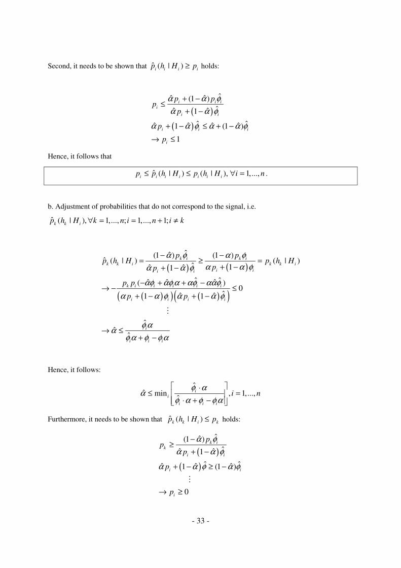
Second, it needs to be shown that ˆ ( | ) ≥i i i i
p h H p holds:
( )
( )
ˆˆ ˆ(1 )ˆˆ ˆ1
ˆ ˆˆ ˆ ˆ ˆ1 (1 )
1
i i i
i
i i
i i i
i
p pp
p
p
p
α α φ
α α φ
α α φ α α φ
+ −≤
+ −
+ − ≤ + −
→ ≤
Hence, it follows that
ˆ ( | ) ( | ), 1,...,i i i i i i i
p p h H p h H i n≤ ≤ ∀ = .
b. Adjustment of probabilities that do not correspond to the signal, i.e.
ˆ ( | ), 1,..., ; 1,..., 1;k k i
p h H k n i n i k∀ = = + ≠
( ) ( )
( )( ) ( )( )
ˆˆ(1 ) (1 )ˆ ( | ) ( | )
ˆ 1ˆ ˆ1
ˆ ˆˆ ˆ ˆ( )0
ˆˆ ˆ1 1
ˆˆ
ˆ
k i k i
k k i k k i
i ii i
k i i i i i
i i i i
i
i i i
p pp h H p h H
pp
p p
p p
α φ α φ
α α φα α φ
αφ αφ α αφ ααφ
α α φ α α φ
φ αα
φ α φ φ α
− −= ≥ =
+ −+ −
− + + −→ − ≤
+ − + −
→ ≤+ −
⋮
Hence, it follows:
ˆˆ min , 1,...,
ˆ
⋅≤ =
⋅ + −
i
i
i i i
i nφ α
αφ α φ φ α
Furthermore, it needs to be shown that ˆ ( | ) ≤k k i k
p h H p holds:
( )
( )
ˆˆ(1 )ˆˆ ˆ1
ˆ ˆˆ ˆ ˆ1 (1 )
0
−≥
+ −
+ − ≥ −
→ ≥
⋮
k i
k
i i
i i
i
pp
p
p
p
α φ
α α φ
α α φ α φ
- 34 -
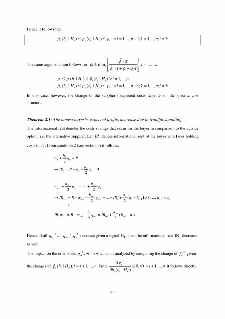
Hence it follows that
ˆ( | ) ( | ) , 1,..., 1; 1,..., ;k k i k k i k
p h H p h H p i n k n i k≤ ≤ ∀ = + = ≠
The same argumentation follows for ˆ
ˆ min , 1,...,ˆ
⋅≥ =
⋅ + −
i
i
i i i
i nφ α
αφ α φ φ α
:
ˆ( | ) ( | ) 1,...,
ˆ ( | ) ( | ) , 1,..., 1; 1,..., ;i i i i i i i
k k i k k i k
p p h H p h H i n
p h H p h H p i n k n i k
≤ ≤ ∀ =
≤ ≤ ∀ = + = ≠
In this case, however, the change of the supplier’s expected costs depends on the specific cost
structure.
Theorem 2.1: The honest buyer’s expected profits decrease due to truthful signaling.
The informational rent denotes the costs savings that occur for the buyer in comparison to the outside
option, i.e. the alternative supplier. Let i
IR denote informational rent of the buyer who faces holding
costs of i
h . From condition 2 (see section 3) it follows:
( )
( )
1 11 1
11 1 1 1 1
11 1 1 1
2
02
2 2
... 0,2 2
...2 2
n
n n
n
n n n
n n
n n n n
n n
n n n n n n n n
i i
i i i i i i
hw q R
hIR R w q
h hw q w q
h qIR R w q IR h h as h h
h qIR R w q IR h h
− −− −
−− − − − −
++ + + +
+ =
→ = − − =
+ = +
→ = − − = = + − > <
= = − − = + −
⋮
Hence, if all 1 1,..., ,k k k
i n nq q q+ − decrease given a signal kH , then the informational rent iIR decreases
as well.
The impact on the order sizes , 1,...,k
mq m i n= + is analyzed by computing the change of k
mγ given
the changes of ˆ ( | ), 1,...,t t k
p h H t i n= + . From 0, 1,...,ˆ ( | )
k
m
t t k
t i np h H
γ∂≤ ∀ = +
∂ it follows directly
- 35 -
that *k
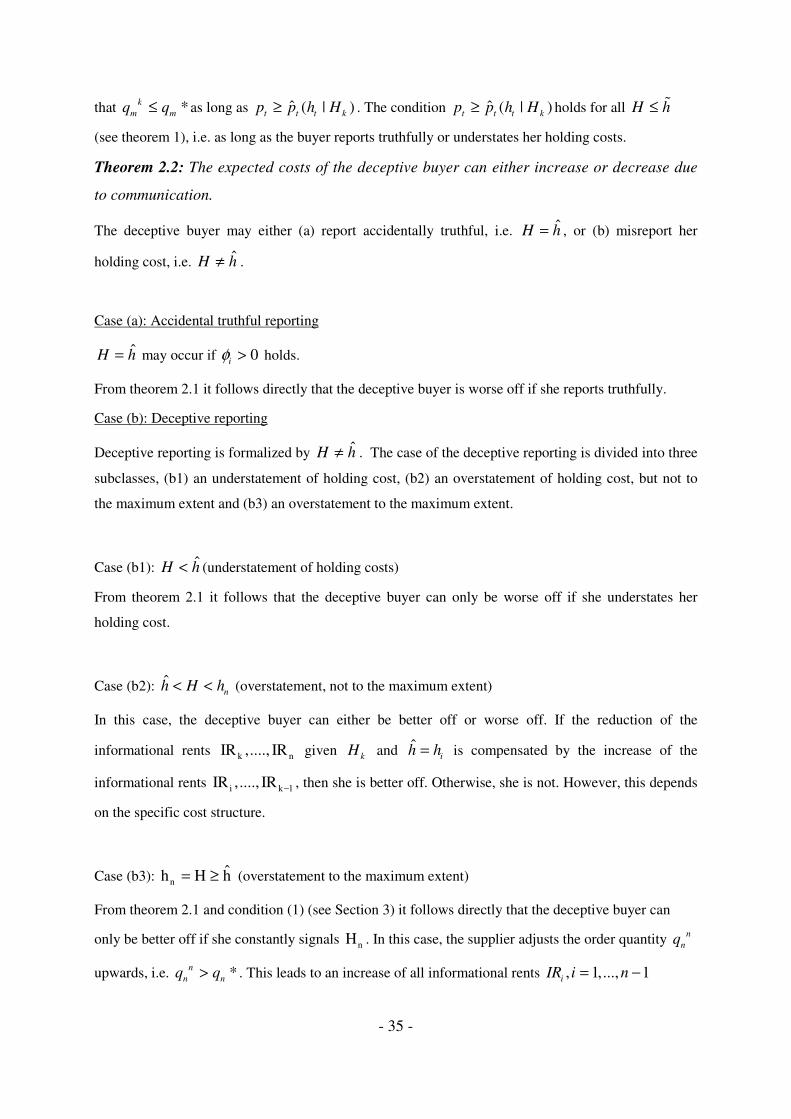
m mq q≤ as long as ˆ ( | )
t t t kp p h H≥ . The condition ˆ ( | )
t t t kp p h H≥ holds for all H h≤ ɶ
(see theorem 1), i.e. as long as the buyer reports truthfully or understates her holding costs.
Theorem 2.2: The expected costs of the deceptive buyer can either increase or decrease due
to communication.
The deceptive buyer may either (a) report accidentally truthful, i.e. ˆH h= , or (b) misreport her
holding cost, i.e. ˆH h≠ .
Case (a): Accidental truthful reporting
ˆH h= may occur if 0i
φ > holds.
From theorem 2.1 it follows directly that the deceptive buyer is worse off if she reports truthfully.
Case (b): Deceptive reporting
Deceptive reporting is formalized by ˆH h≠ . The case of the deceptive reporting is divided into three
subclasses, (b1) an understatement of holding cost, (b2) an overstatement of holding cost, but not to
the maximum extent and (b3) an overstatement to the maximum extent.
Case (b1): ˆH h< (understatement of holding costs)
From theorem 2.1 it follows that the deceptive buyer can only be worse off if she understates her
holding cost.
Case (b2): ˆn
h H h< < (overstatement, not to the maximum extent)
In this case, the deceptive buyer can either be better off or worse off. If the reduction of the
informational rents k nIR ,...., IR given k
H and ˆi
h h= is compensated by the increase of the
informational rents i k 1IR ,...., IR − , then she is better off. Otherwise, she is not. However, this depends
on the specific cost structure.
Case (b3): nˆh H h= ≥ (overstatement to the maximum extent)
From theorem 2.1 and condition (1) (see Section 3) it follows directly that the deceptive buyer can
only be better off if she constantly signals nH . In this case, the supplier adjusts the order quantity n
nq
upwards, i.e. *n
n nq q> . This leads to an increase of all informational rents , 1,..., 1
iIR i n= −

- 36 -
Theorem 3.2: As long as ( )
,
,
1
k i
i k i i i i
i k i k i
critk i
i k i i i i
i k i k i
p CD p CD
p CD p CD
φ φ
α αφ φ
≠
≠
∆ + ∆
≥ =∆ − − ∆
∑∑ ∑
∑∑ ∑ holds,
communication enhances the supply chain performance.
( )
( )
( )
( )
,
,
,
,
,
1
1 0
1
1
k i
i k i i i
i k i k i
i
i i i
i
k i
i k i i i i
i k i k i
k i
i k i i i i
i k i k i
k i
i k i i i i
i k i k i
critk i
i k i i i i
i k i k i
CD p CD p CD
p CD
p CD p CD
p CD p CD
p CD p CD
p CD p CD
α φ α
α φ
φ φ
α φ α φ
φ φ
α αφ φ
≠
≠
≠
≠
≠
∆ = − ∆ + ∆
+ − ∆ ≤
∆ + ∆
≤
∆ − − ∆
∆ + ∆
≥ =∆ − − ∆
∑∑ ∑
∑
∑∑ ∑
∑∑ ∑
∑∑ ∑
∑∑ ∑
⋮
⋮
As 0i
iCD∆ ≤ it can be easily shown that 1
kritα ≤ holds.
Theorem 3.3: Given a certain probability that the supplier interacts with an honest buyer, i.e.
α , it is more likely that communication is an appropriate coordination mechanism if the
supplier’s trust in the buyer’s signal decrease, i.e. if α̂ decrease.
If critα = α holds, it follows that 0CD∆ = (see theorem 3.2). Additionally, 0CD
α
∂∆≤
∂.
( )
( )
( )
,
,
,
1
1
0
1
k i
i k i i i
i k i k i
i
i i i
i
k i
i k i i i
i k i k i
i
i i i
i
i k
i i i i k i
i i k i k
CD p CD p CD
p CD
CDp CD p CD
p CD
p CD p CD
α φ α
α φ
φα
φ
φ φ
≠
≠
≠
∆ = − ∆ + ∆
+ − ∆
∂∆= − ∆ + ∆
∂
− ∆ ≤
− ∆ ≤ ∆
∑∑ ∑
∑
∑∑ ∑
∑
∑ ∑∑⋮
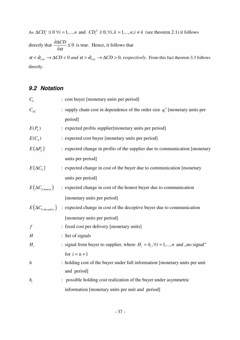
- 37 -
As 0 1,...,i
iCD i n∆ ≤ ∀ = and 0, , 1,..., ;k
iCD i k n i k≥ ∀ = ≠ (see theorem 2.1) it follows
directly that 0CD
α
∂∆≤
∂ is true. Hence, it follows that
ˆ ˆ0 0, .crit crit
CD and CD respectivelyα α α α< → ∆ < > → ∆ > From this fact theorem 3.3 follows
directly.
9.2 Notation
bC : cost buyer [monetary units per period]
SCC : supply chain cost in dependence of the order size k
iq [monetary units per
period]
( )S
E P : expected profits supplier[monetary units per period]
( )b
E C : expected cost buyer [monetary units per period]
( )SE P∆ : expected change in profits of the supplier due to communication [monetary
units per period]
( )bE C∆ : expected change in cost of the buyer due to communication [monetary
units per period]
( ),b honestE C∆ : expected change in cost of the honest buyer due to communication
[monetary units per period]
( ),b deceptiveE C∆ : expected change in cost of the deceptive buyer due to communication
[monetary units per period]
f : fixed cost per delivery [monetary units]
H : Set of signals
iH : signal from buyer to supplier, where , 1,...,
i iH h i n= ∀ = and „no signal“
for i n 1= +
h : holding cost of the buyer under full information [monetary units per unit
and period]
ih : possible holding cost realization of the buyer under asymmetric
information [monetary units per unit and period]

- 38 -
hɶ : actual holding cost of the buyer in a period [monetary units per unit and
period]
iIR : informational rent of the buyer facing holding cost
ih , 1,...,i n= [monetary
units per unit and period]
SP : profit supplier [monetary units per period]
ip : a-priori probability that the buyer faces holding cost
ih , 1,...,i n=
( | )i i k
p h H : actual a-posteriori probability, 1,...,i n= ; 1,..., 1k n= +
ˆ ( | )i i k
p h H : perceived a-posteriori probability k
H ; 1,...,i n= ; 1,..., 1k n= +
( )i i k
p h H∩ : actual conjoint probability distribution; 1,...,i n= ; 1,..., 1k n= +
q : order size [quantity unit]
iq : order size that corresponds to the holding cost realization
ih , i=1,…,n
[quantity unit]
*i
q : optimal order size (w.r.t. problem AI) that corresponds to the holding
cost realization i
h , i=1,…,n [quantity unit]
, *i SC
q : supply chain optimal order size that corresponds to the holding cost
realization i
h , i=1,…,n [quantity unit]
k
iq : optimal order size (w.r.t. problem AI) that corresponds to the holding cost
realization i
h , i=1,…,n and is calculated w.r.t. ˆ ( | )i i k
p h H ,
1,..., ; 1,..., 1i n k n= = + [quantity unit]
minq : minimum order size under which the supplier yields (positive) profits
[quantity unit]
R : cost of the outside option [monetary units]
w : wholesale price under full information [monetary units]
iw : wholesale price that corresponds to holding cost realization
ih , 1,...,i n= ;
[monetary units]
*i
w : optimal wholesale price (w.r.t. problem AI) that corresponds to holding
cost realization i
h , 1,...,i n= [monetary units]
*SC
w : supply chain optimal wholesale price under full information [monetary
units]
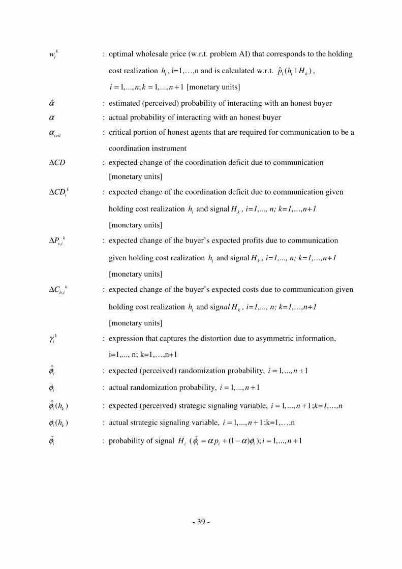
- 39 -
k
iw : optimal wholesale price (w.r.t. problem AI) that corresponds to the holding
cost realization i
h , i=1,…,n and is calculated w.r.t. ˆ ( | )i i k
p h H ,
1,..., ; 1,..., 1i n k n= = + [monetary units]
α̂ : estimated (perceived) probability of interacting with an honest buyer
α : actual probability of interacting with an honest buyer
critα : critical portion of honest agents that are required for communication to be a
coordination instrument
CD∆ : expected change of the coordination deficit due to communication
[monetary units]
k
iCD∆ : expected change of the coordination deficit due to communication given
holding cost realization i
h and signalk
H , i=1,..., n; k=1,…,n+1
[monetary units]
,k
s iP∆ : expected change of the buyer’s expected profits due to communication
given holding cost realization i
h and signalk
H , i=1,..., n; k=1,…,n+1
[monetary units]
,k
b iC∆ : expected change of the buyer’s expected costs due to communication given
holding cost realization i
h and signalk
H , i=1,..., n; k=1,…,n+1
[monetary units]
k
iγ : expression that captures the distortion due to asymmetric information,
i=1,..., n; k=1,…,n+1
ˆi
φ : expected (perceived) randomization probability, 1,..., 1i n= +
iφ : actual randomization probability, 1,..., 1i n= +
ˆ ( )i k
hφ : expected (perceived) strategic signaling variable, 1,..., 1i n= + ;k=1,…,n
( )i k
hφ : actual strategic signaling variable, 1,..., 1i n= + ;k=1,…,n
iφɶ : probability of signal
iH ( (1 )
i i ipφ α α φ= + −ɶ ); 1,..., 1i n= +