1

Chapter Two

Supply and Demand

© 2009 Pearson Addison-Wesley. All rights reserved. 2-2

Chapter Outline

1. Demand. 2. Supply. 3. Market Equilibrium. 4. Shocking the Equilibrium. 5. Effects of Government

Interventions. 6. When to Use the Supply-and-

Demand Model.

© 2009 Pearson Addison-Wesley. All rights reserved. 2-3

Demand: determinants of demand.

The following factors determine the demand for a good:

Price of the goodTastesInformationPrices of related goods

Complements and substitutesIncomeGovernment rules and regulationsOther

2

© 2009 Pearson Addison-Wesley. All rights reserved. 2-4

Demand: the demand curve

Quantity demanded - the amount of a good that consumers are willing to buy at a given price, holding constant the other factors that influence purchases.Demand curve - the quantity demanded at each possible price, holding constant the other factors that influence purchases

© 2009 Pearson Addison-Wesley. All rights reserved. 2-5

Figure 2.1 A Demand Curve

Law of Demandconsumers demand more of a good the

lower its price, holding constant all other

factors that influence consumption

p, $

per

kg

200 220

Demand curve for pork, D1

240 286Q, Million kg of pork per year

0

2.303.304.30

14.30

© 2009 Pearson Addison-Wesley. All rights reserved. 2-6

Figure 2.2 A Shift of the Demand Curve

p, $

per

kg

220176

Effect of a 60¢ increase in the price of beef

D1

D2

232Q, Million kg of pork per year

0

3.30

3

© 2009 Pearson Addison-Wesley. All rights reserved. 2-7

The Demand Function

The processed pork demand function is:

Q = D(p, pb, pc, Y)

where Q is the quantity of pork demandedp is the price of pork (dollars per kg)

pb is the price of beef (dollars per kg)pc is the price of chicken (dollars per kg)

Y is the income of consumers (thousand dollars)

© 2009 Pearson Addison-Wesley. All rights reserved. 2-8

From the Demand Function to the Demand Curve

Estimated demand function for pork:

Q = 171−20p + 20pb + 3pc + 2Y

Using the values pb = 4, pc = 3.33 and Y = 12.5, we have

Q = 286−20p

which is the linear demand function for pork.

© 2009 Pearson Addison-Wesley. All rights reserved. 2-9

From the Demand Function to the Demand Curve

If p = 0, thenQ = 286p,

$ p

er k

g

200 220

Demand curve for pork, D1

240 286Q, Million kg of pork per year

0

2.303.304.30

14.30

Q = 286−20pIf p increases by

$1 (to $4.30) then,

Q = 200

If p decreasesby $1 (to$2.30) then,

Q = 240

In general, ΔQ = -20Δp

= slope Δp

If p = $3.30 then,

Q = 220

4

© 2009 Pearson Addison-Wesley. All rights reserved. 2-10

Solved Problem 2.1

How much would the price have to fall for consumers to be willing to buy 1 million more kg of pork per year?

© 2009 Pearson Addison-Wesley. All rights reserved. 2-11

Solved Problem 2.1: Answer

1. Express the price that consumers are willing to pay as a function of quantity.

Q = 286−20p

20p = 286 - Q

p = 14.30 − 0.05Q

© 2009 Pearson Addison-Wesley. All rights reserved. 2-12

Solved Problem 2.1: Answer

2. Use the inverse demand curve to determine how much the price must change for consumers to buy 1 million more kg of pork per year.

Δp = p2 − p1= (14.30 − 0.05Q2) − (14.30 − 0.05Q1)= –0.05(Q2 − Q1)= –0.05ΔQ.

The change in quantity is ΔQ = Q2 − Q1 = (Q1 + 1)−Q1 = 1, so the change in price is Δp = –0.05.

5

© 2009 Pearson Addison-Wesley. All rights reserved. 2-13

Application: Aggregating the Demand for Broadband Service

© 2009 Pearson Addison-Wesley. All rights reserved. 2-14

Supply: determinants of supply.

The following factors determine the supply for a good:

Price of the goodCostsGovernment rules and regulations

© 2009 Pearson Addison-Wesley. All rights reserved. 2-15

Supply: the demand curve

Quantity supplied - the amount of a good that firms want to sell at a given price, holding constant other factors that influence firms’ supply decisions, such as costs and government actionsSupply curve - the quantity supplied at each possible price, holding constant the other factors that influence firms’supply decisions

6

© 2009 Pearson Addison-Wesley. All rights reserved. 2-16

Figure 2.3 A Supply Curve

p, $

per

kg

220176

Supply curve, S1

300Q, Million kg of pork per year

0

3.30

5.30

An increase in the price…

causes a movement along the curve….

and a decrease in the quantity supplied….

© 2009 Pearson Addison-Wesley. All rights reserved. 2-17

Figure 2.4 A Shift of a Supply Curve

p , $

per

kg

205176

S 1S2

220Q, Million kg of pork per year

0

3.30

A $0.25 increase in the price of hogs….. shifts the supply curve

to the left

reducing the quantity supplied at the previous price.

© 2009 Pearson Addison-Wesley. All rights reserved. 2-18

The Supply Function

The processed pork supply function is:

Q = S(p, ph)

where Q is the quantity of pork suppliedp is the price of pork (dollars per kg)

ph is the price of a hog (dollars per kg)

7

© 2009 Pearson Addison-Wesley. All rights reserved. 2-19

From the Supply Function to the Supply Curve

Estimated demand function for pork:

Q = 178 + 40p−60ph

Using the values ph = $1.50 per kg

Q = 88 + 40p.

What happens to the quantity supplied if theprice of processed pork increases by Δp = p2−p1?

© 2009 Pearson Addison-Wesley. All rights reserved. 2-20

Figure 2.5 Total Supply: The Sum of Domestic and Foreign Supply

© 2009 Pearson Addison-Wesley. All rights reserved. 2-21

Solved Problem 2.2

How does a quota set by the United States on foreign steel imports of Qaffect the total American supply curve for steel given the domestic supply, Sd in panel a of the graph, and foreign supply, Sf in panel b?

8

© 2009 Pearson Addison-Wesley. All rights reserved. 2-22

Solved Problem 2.2

© 2009 Pearson Addison-Wesley. All rights reserved. 2-23

Market Equilibrium

Equilibrium - a situation in which no one wants to change his or her behavior.

excess demand the amount by which the quantity demanded exceeds the quantity supplied at a specified price.excess supply the amount by which the quantity supplied is greater than the quantity demanded at a specified price

© 2009 Pearson Addison-Wesley. All rights reserved. 2-24

Figure 2.6 Market Equilibrium

p, $

per

kg

220176

D

S

e

233 246194 207Q, Million kg of pork per year

0

3.95

3.30

2.65

Excess supply = 39

Excess demand = 39

Market equilibrium point!

At a price below equilibrium….

the quantity supplied….

is below the quantity demanded

At a price above equilibrium….

the quantity demanded….

is below the quantity supplied

9

© 2009 Pearson Addison-Wesley. All rights reserved. 2-25

Using Math to Determine the Equilibrium

Demand: Qd = 286 − 20pSupply: Qs = 88 + 40pEquilibrium:

Qd = Qs

286 − 20p = 88 + 40p60p = 198P = $3.30Q = 286 – 20(3.3) = 220

© 2009 Pearson Addison-Wesley. All rights reserved. 2-26

Equilibrium: Practice Problem

The demand function for a good is Q = a−bp, and the supply function is Q = c + ep, where a, b, c, and e are positive constants. Solve for the equilibrium price and quantity in terms of these four constants.

© 2009 Pearson Addison-Wesley. All rights reserved. 2-27

Shocking the Equilibrium

The equilibrium changes only if a shock occurs that shifts the demand curve or the supply curve. These curves shift if one of the variables we were holding constant

changes.

10

© 2009 Pearson Addison-Wesley. All rights reserved. 2-28

Figure 2.7a Equilibrium Effects of a Shift of a Demand Curve

D1

D2

S

1760 220 228 232

Q, Million kg of pork per year

Excess demand = 12

3.303.50

e2

e1

p, $

per

kg

A $0.60 increase in the price of beef shifts the demand outward

At the original price there is now an excess demand….

Which puts an upward pressure in the price to a new equilibrium.

© 2009 Pearson Addison-Wesley. All rights reserved. 2-29

Figure 2.7b Equilibrium Effects of a Shift of a Supply Curve

S1S2

Q, Million kg of pork per year

3.303.55

e1

e2

D

p, $

per

kg

1760 220205 215

Excess demand = 15

A $0.25 increase in the price of hogs shifts the supply curve to the left

At the original price there is now an excess demand….

Which puts an upward pressure in the price to a new equilibrium.

© 2009 Pearson Addison-Wesley. All rights reserved. 2-30

Solved Problem 2.3

Mathematically, how does the equilibrium price of pork vary as the price of hogs changes if the variables that affect demand are held constant at their typical values?

11

© 2009 Pearson Addison-Wesley. All rights reserved. 2-31

Solved Problem 2.3: Solution

1. Solve for the equilibrium price of pork in terms of the price of hogs.

Qd = 286−20pQs = 178 + 40p−60ph286−20p = 178 + 40p−60ph60p = 108 – 60php = 1.8 – ph

2. Show how the equilibrium price of pork varies with the price of hogs.

Since Δp = Δph, any increase in the price of hogs causes an equal increase in the price of processed pork.

© 2009 Pearson Addison-Wesley. All rights reserved. 2-32

Solved Problem 2.4

In the first few weeks after the U.S. ban, the quantity of beef sold in Japan fell substantially, and the price rose. In contrast, three weeks after the first discovery, the U.S. price in January 2004 fell by about 15% and the quantity sold increased by 43% over the last week in October 2003. Use supply-and-demand diagrams to explain why these events occurred.

© 2009 Pearson Addison-Wesley. All rights reserved. 2-33

Solved Problem 2.4

12

© 2009 Pearson Addison-Wesley. All rights reserved. 2-34

Figure 2.8 A Ban on Rice Imports Raises the Price in Japan

p, P

r ice

ofric

e pe

r pou

nd

Q2 Q1

S (no ban)

D

Q, Tons of rice per year

p2 e2

e1p1

S (ban)– A ban on rice imports

shifts the total supply of rice in Japan…

which causes the equilibrium to change and the price to increase.

© 2009 Pearson Addison-Wesley. All rights reserved. 2-35

Solved Problem 2.5

What is the effect of a United States quota on steel of Q on the equilibrium in the U.S. steel market? Hint: The answer depends on whether the quota binds (is low enough to affect the equilibrium).

© 2009 Pearson Addison-Wesley. All rights reserved. 2-36

Solved Problem 2.5

13

© 2009 Pearson Addison-Wesley. All rights reserved. 2-37

Figure 2.9 Price Ceiling on Gasoline

p, $

per

gal

lon

Qs Q1= Qd

Price ceiling

S1

D

S2

Q, Gallons of gasoline per monthExcess demand

e1p1= p–

Supply shifts to the left….

p1

but gas stations must continue to charge a price of P1…..

which creates an excess demand.

© 2009 Pearson Addison-Wesley. All rights reserved. 2-38

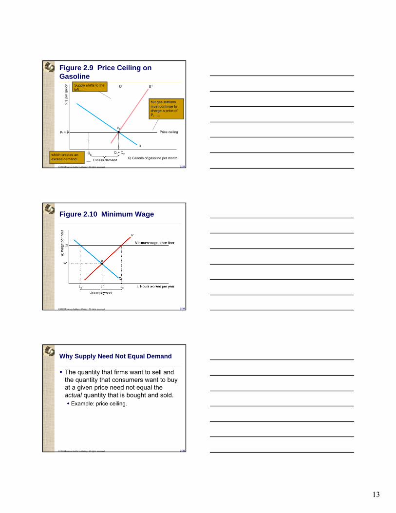
Figure 2.10 Minimum Wage

© 2009 Pearson Addison-Wesley. All rights reserved. 2-39

Why Supply Need Not Equal Demand

The quantity that firms want to sell and the quantity that consumers want to buy at a given price need not equal the actual quantity that is bought and sold.

Example: price ceiling.

14

© 2009 Pearson Addison-Wesley. All rights reserved. 2-40

Perfectly competitive markets

Everyone is a price taker.

Firms sell identical products.

Everyone has full information about the price and quality of goods.

Costs of trading are low.

© 2009 Pearson Addison-Wesley. All rights reserved. 2-41

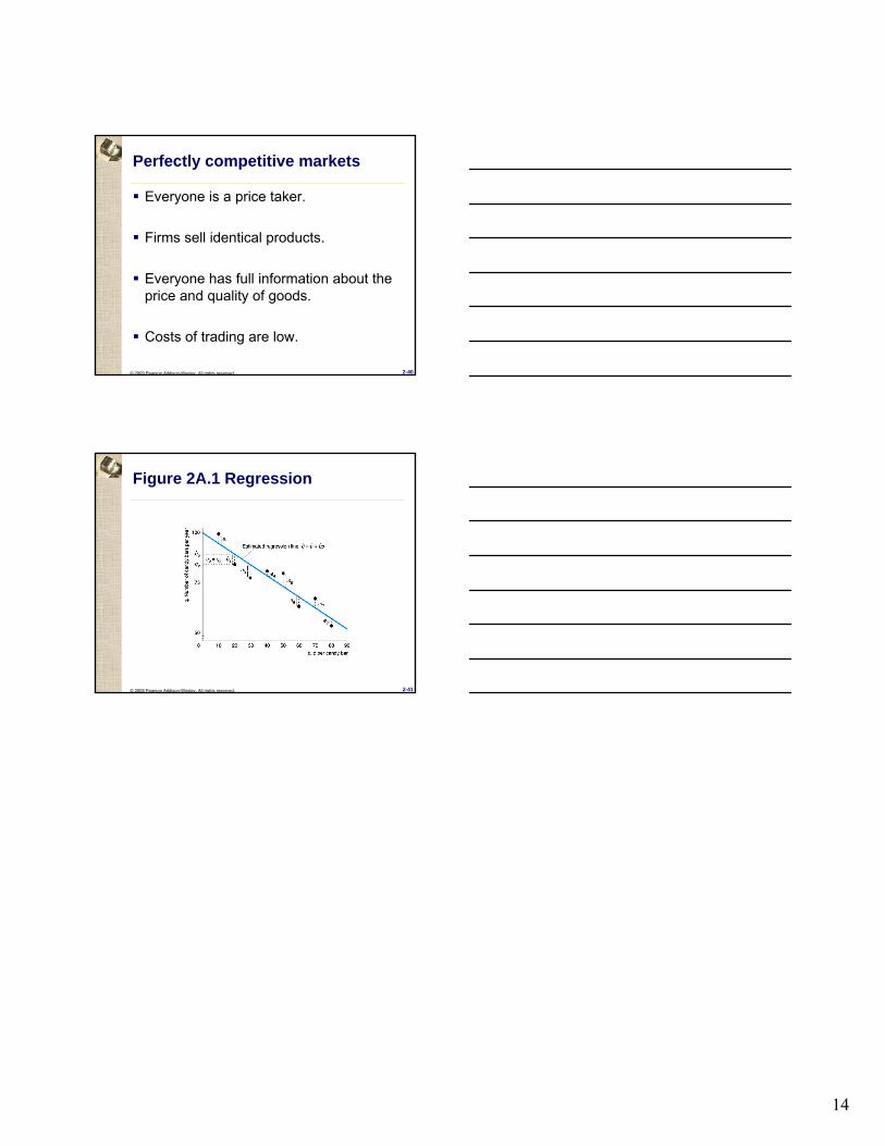
Figure 2A.1 Regression