SupplementaryInformation,for:, … · ! 1"of9" SupplementaryInformation,for:,, Strandseparationestablishes,asustained,lockattheTus–Ter$replicationfork barrier, BojkA.Berghuis1,"David"Dulin1,Zhi:Qiang"Xu2,"Theo"van"Laar1,Bronwen"Cross1,"Richard"Janissen1,

1 of 9

Supplementary Information for:

Strand separation establishes a sustained lock at the Tus–Ter replication fork barrier

Bojk A. Berghuis1, David Dulin1, Zhi-‐Qiang Xu2, Theo van Laar1, Bronwen Cross1, Richard Janissen1, Slobodan Jergic2, Nicholas E. Dixon2, Martin Depken1 & Nynke H. Dekker1*

1Department of Bionanoscience, Kavli institute of Nanoscience, Delft University of Technology, Lorentzweg 1,

2628 CJ Delft, The Netherlands 2Centre for Medical and Molecular Bioscience and School of Chemistry, University of Wollongong, New South

Wales 2522, Australia * Correspondence may be addressed to [email protected].

Supplementary Results

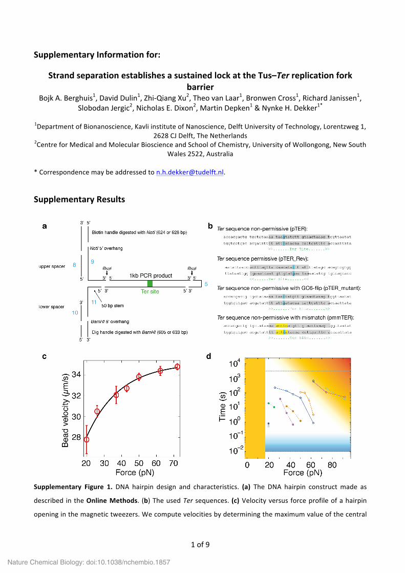
Supplementary Figure 1. DNA hairpin design and characteristics. (a) The DNA hairpin construct made as

described in the Online Methods. (b) The used Ter sequences. (c) Velocity versus force profile of a hairpin

opening in the magnetic tweezers. We compute velocities by determining the maximum value of the central

Nature Chemical Biology: doi:10.1038/nchembio.1857

2 of 9

derivative of the extension versus time traces, i.e. the instantaneous apparent velocity upon lock rupture.

Each data point in the figure is the average of hundreds of rupture events (the data here are from ~104

rupture events). The data have been fit with a single exponential (black line) to provide a guide to the eye.

Note that our computations only provide a lower bound to the velocity, since our 100 Hz sampling frequency

is not sufficiently high to capture the opening dynamics over a typical distance of ~0.6 µm (500 bp opening).

Nonetheless, these lower bounds suffice to indicate that the hairpin-‐opening rate exceeds the DNA

unwinding rate of the E. coli replisome by at least 10-‐fold at 20 pN force. (d) Here we visualize the constraints

on the experimental time–force window due to biological (orange) or instrumentation (blue) limits. The data,

identical to Figure 3c, is added as a frame of reference. Below ~16 pN, base-‐paired DNA is energetically more

favorable, therefore the hairpin remains closed (orange fill). With an acquisition rate of 100 Hz, the cutoff

time is in principle 10–2 s (black dashed line); however, the error already becomes relatively large for lock

lifetimes shorter than 0.1 s (blue gradient). Measurements are further limited by the lifetime of the DNA

hairpin since DNA tethering relies on electrostatic interactions. This implies that very long measurement

times, high forces or a combination of both (orange gradient) should be avoided. Typically we avoided having

to measure lifetimes exceeding an hour (grey dashed line). Here we are able to see that the force–lifetime

behavior exhibited by wt Tus already approaches the limits of the assay.


3 of 9

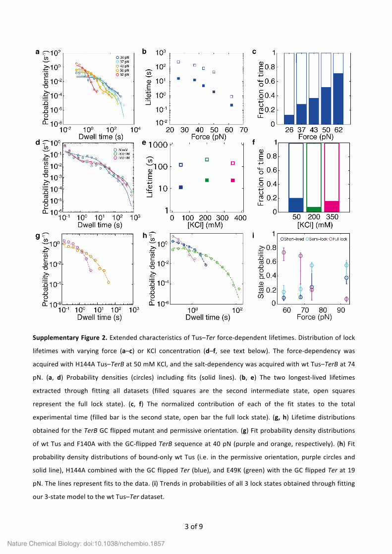
Supplementary Figure 2. Extended characteristics of Tus–Ter force-‐dependent lifetimes. Distribution of lock

lifetimes with varying force (a–c) or KCl concentration (d–f, see text below). The force-‐dependency was

acquired with H144A Tus–TerB at 50 mM KCl, and the salt-‐dependency was acquired with wt Tus–TerB at 74

pN. (a, d) Probability densities (circles) including fits (solid lines). (b, e) The two longest-‐lived lifetimes

extracted through fitting all datasets (filled squares are the second intermediate state, open squares

represent the full lock state). (c, f) The normalized contribution of each of the fit states to the total

experimental time (filled bar is the second state, open bar the full lock state). (g, h) Lifetime distributions

obtained for the TerB GC flipped mutant and permissive orientation. (g) Fit probability density distributions

of wt Tus and F140A with the GC-‐flipped TerB sequence at 40 pN (purple and orange, respectively). (h) Fit

probability density distributions of bound-‐only wt Tus (i.e. in the permissive orientation, purple circles and

solid line), H144A combined with the GC flipped Ter (blue), and E49K (green) with the GC flipped Ter at 19

pN. The lines represent fits to the data. (i) Trends in probabilities of all 3 lock states obtained through fitting

our 3-‐state model to the wt Tus–Ter dataset.


4 of 9

Salt-‐dependence of Tus–Ter lock

As the reported dissociation constant (KD) of the Tus–dsTerB complex has been shown to be highly salt-‐

dependent, we investigated whether lock formation also exhibits a strong salt dependence. We observed

that the fraction of rupture events recorded with a lifetime below our cutoff time of 10–2 s (i.e., the fraction

of open hairpins at t = 0 s) increased from 0% at 50 mM to 14% at 350 mM KCl, while during these

experiments care was taken to keep [Tus] well above (at least an order of magnitude) the reported salt-‐

dependent KD, thereby ensuring the continuous binding of Tus to Ter. Concomitantly, we observed that the

lifetimes of the two longest-‐lived exponentials for wt Tus remain virtually unaffected when increasing the

[KCl] from 50 to 350 mM, indicating that the lock strength is hardly affected by salt concentration

(Supplementary Fig. 2d–f). In contrast, the reported KD of the Tus–dsTerB complex increases from ~10–13 to

~10–8 M within the 50 to 350 mM range. We conclude from this that the rate of lock formation is slightly

affected by ionic screening, but once the lock is formed its strength remains unaffected. This is in accord with

SPR data.


5 of 9

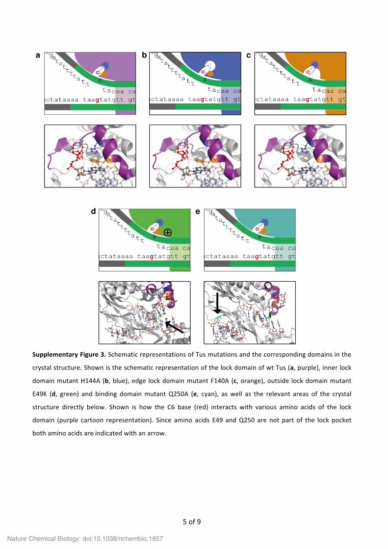
Supplementary Figure 3. Schematic representations of Tus mutations and the corresponding domains in the

crystal structure. Shown is the schematic representation of the lock domain of wt Tus (a, purple), inner lock

domain mutant H144A (b, blue), edge lock domain mutant F140A (c, orange), outside lock domain mutant

E49K (d, green) and binding domain mutant Q250A (e, cyan), as well as the relevant areas of the crystal

structure directly below. Shown is how the C6 base (red) interacts with various amino acids of the lock

domain (purple cartoon representation). Since amino acids E49 and Q250 are not part of the lock pocket

both amino acids are indicated with an arrow.


6 of 9

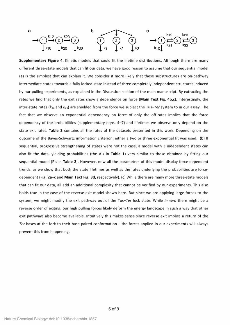
Supplementary Figure 4. Kinetic models that could fit the lifetime distributions. Although there are many

different three-‐state models that can fit our data, we have good reason to assume that our sequential model

(a) is the simplest that can explain it. We consider it more likely that these substructures are on-‐pathway

intermediate states towards a fully locked state instead of three completely independent structures induced

by our pulling experiments, as explained in the Discussion section of the main manuscript. By extracting the

rates we find that only the exit rates show a dependence on force (Main Text Fig. 4b,c). Interestingly, the

inter-‐state rates (k12 and k23) are shielded from the force we subject the Tus–Ter system to in our assay. The

fact that we observe an exponential dependency on force of only the off-‐rates implies that the force

dependency of the probabilities (supplementary eqns. 4–7) and lifetimes we observe only depend on the

state exit rates. Table 2 contains all the rates of the datasets presented in this work. Depending on the

outcome of the Bayes-‐Schwartz information criterion, either a two or three exponential fit was used. (b) If

sequential, progressive strengthening of states were not the case, a model with 3 independent states can

also fit the data, yielding probabilities (the A’s in Table 1) very similar to those obtained by fitting our

sequential model (P’s in Table 2). However, now all the parameters of this model display force-‐dependent

trends, as we show that both the state lifetimes as well as the rates underlying the probabilities are force-‐

dependent (Fig. 2a–c and Main Text Fig. 3d, respectively). (c) While there are many more three-‐state models

that can fit our data, all add an additional complexity that cannot be verified by our experiments. This also

holds true in the case of the reverse-‐exit model shown here. But since we are applying large forces to the

system, we might modify the exit pathway out of the Tus–Ter lock state. While in vivo there might be a

reverse order of exiting, our high pulling forces likely deform the energy landscape in such a way that other

exit pathways also become available. Intuitively this makes sense since reverse exit implies a return of the

Ter bases at the fork to their base-‐paired conformation – the forces applied in our experiments will always

prevent this from happening.


7 of 9

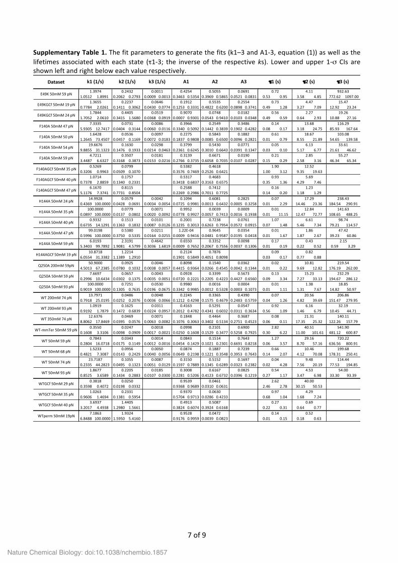
Supplementary Table 1. The fit parameters to generate the fits (k1–3 and A1-‐3, equation (1)) as well as the lifetimes associated with each state (τ1-‐3; the inverse of the respective ks). Lower and upper 1-‐σ CIs are shown left and right below each value respectively.

Dataset

WTperm'50mM'19pN

WTGCf'50mM'40'pN

WTGCf'50mM'35'pN

WTGCf'50mM'29'pN

WT'50mM'93'pN

WT'50mM'74'pN

WT'50mM'68'pN

WT'50mM'59'pN

WT7mmTer'50mM'59'pN

WT'350mM'74'pN

WT'200mM'93'pN

WT'200mM'74'pN

Q250A'50mM'93'pN

Q250A'50mM'59'pN

Q250A'200mM'59pN

H144AGCf'50mM'19'pN

H144A'50mM'59'pN

H144A'50mM'47'pN

H144A'50mM'40'pN

H144A'50mM'35'pN

H144A'50mM'24'pN

F140AGCf'50mM'47'pN

F140AGCf'50mM'40'pN

F140AGCf'50mM'35'pN

F140A'50mM'59'pN

F140A'50mM'54'pN

F140A'50mM'50'pN

F140A'50mM'47'pN

E49KGCf'50mM'24'pN

E49KGCf'50mM'19'pN

E49K'50mM'59'pN 1.0512 1.8991 0.2062 0.2793 0.0009 0.0013 0.3463 0.5354 0.3969 0.5865 0.0521 0.0831

0.7784 2.0261 0.1411 0.3062 0.0430 0.0774 0.1253 0.3331 0.4822 0.6200 0.0898 0.3741

1.7052 2.0610 0.3415 1.5680 0.0368 0.0919 0.0007 0.9301 0.0543 0.9410 0.0103 0.0348

5.9305 12.7417 0.0404 0.3144 0.0060 0.0116 0.3340 0.5092 0.1442 0.3839 0.1902 0.4282

1.2645 73.4507 0.0457 0.1169 0.0072 0.0183 0.1837 0.9808 0.0085 0.6500 0.0096 0.2821

9.8855 31.1323 0.1476 0.1933 0.0214 0.0463 0.2361 0.6245 0.3010 0.6643 0.0391 0.1347

3.4487 6.6327 0.3168 0.3873 0.0153 0.0216 0.2766 0.3735 0.6058 0.7035 0.0107 0.0287

0.3206 0.9963 0.0509 0.1070 0.3576 0.7469 0.2526 0.6421

0.7378 2.8859 0.1340 0.2331 0.3418 0.6837 0.3163 0.6575

5.1176 7.3741 0.7731 0.8504 0.2269 0.2986 0.7011 0.7725

0.4369 100.0000 0.0428 0.0691 0.0034 0.0054 0.0725 0.9981 0.0013 0.6432 0.0005 0.3258

0.0897 100.0000 0.0137 0.0802 0.0020 0.0092 0.0778 0.9927 0.0057 0.7413 0.0016 0.1938

0.6735 14.1291 0.1363 0.1832 0.0087 0.0126 0.1235 0.3013 0.6263 0.7954 0.0572 0.0915

0.5996 100.0000 0.3750 0.5335 0.0164 0.0255 0.0009 0.9416 0.0481 0.9587 0.0195 0.0418

5.3403 99.7892 1.9081 4.5799 0.3036 1.6819 0.0009 0.7652 0.2067 0.7556 0.0037 0.1306

6.0554 31.3382 1.1389 1.2910 0.1901 0.5849 0.4051 0.8098

4.5013 67.2385 0.0780 0.1032 0.0038 0.0057 0.4415 0.9364 0.0266 0.4545 0.0042 0.1344

0.2996 10.6434 0.0302 0.1375 0.0035 0.0051 0.0720 0.2221 0.2205 0.4223 0.4427 0.6560

0.9019 100.0000 0.1305 0.7635 0.0196 0.0675 0.3342 0.9985 0.0012 0.5328 0.0003 0.1073

0.7918 25.0195 0.0252 0.2076 0.0036 0.0066 0.1212 0.4298 0.1575 0.4679 0.2483 0.5759

0.9192 1.7879 0.1472 0.6839 0.0224 0.0957 0.2012 0.4782 0.4341 0.6032 0.0311 0.3634

8.8062 17.8469 0.0395 0.0576 0.0063 0.0082 0.1076 0.3063 0.3402 0.5134 0.2751 0.4523

0.1608 3.3106 0.0098 0.0909 0.0017 0.0021 0.0250 0.1608 0.1529 0.3477 0.5258 0.7925

0.2804 16.0718 0.0175 0.1149 0.0012 0.0016 0.0454 0.1429 0.1021 0.2301 0.6691 0.8218

0.4821 7.3087 0.0143 0.2429 0.0040 0.0056 0.0649 0.2198 0.1221 0.3548 0.3953 0.7643

0.2335 44.2823 0.0495 0.1323 0.0051 0.0129 0.1597 0.7889 0.1345 0.6289 0.0323 0.2382

0.8525 3.6589 0.1434 0.2883 0.0107 0.0300 0.2281 0.5206 0.4123 0.6732 0.0396 0.1219

0.3598 0.4072 0.0198 0.0332 0.9368 0.9689 0.0310 0.0631

0.9606 1.4694 0.1381 0.5954 0.5704 0.9713 0.0286 0.4233

3.2017 4.4938 1.2980 1.5661 0.3824 0.6074 0.3924 0.6168

6.8488 100.0000 1.5950 5.4160 0.9176 0.9959 0.0039 0.0823

1.0714 0.1757

0.81156.1670

1.0263 0.2331

1.44053.6937

7.1863 1.9324

0.5317 0.4683

0.74120.2588

0.9370 0.0630

0.50870.4913

0.9528 0.0472

0.0250 0.9539 0.04610.3818

0.2205 0.0185 0.3008 0.6167 0.08251.8677

0.1055 0.0087 0.3150 0.5152 0.169723.7187

0.0956 0.0050 0.0874 0.1887 0.72391.5233

0.0343 0.0014 0.0843 0.1514 0.76430.7843

0.0247 0.0018 0.0998 0.2101 0.69000.3550

0.0469 0.0071 0.1848 0.4464 0.368712.6376

0.1625 0.0311 0.4163 0.5291 0.05471.0919

0.0486 0.0048 0.2245 0.3365 0.439013.7971

0.7251 0.0530 0.9980 0.0016 0.0004100.0000

0.0657 0.0043 0.0928 0.3399 0.56737.6697

0.0925 0.0046 0.8098 0.1540 0.036250.9000

1.2214 0.2124 0.787610.8718

2.3191 0.4642 0.6550 0.3352 0.00986.0193

0.5380 0.0211 1.22E704 0.9645 0.035499.0198

0.1513 0.0101 0.2001 0.7238 0.07610.9332

0.0779 0.0071 0.9952 0.0039 0.0009100.0000

0.0579 0.0042 0.1094 0.6081 0.282514.9928

0.0799 0.5382 0.46180.5269

0.3507 0.0181 0.3139 0.6671 0.01904.7211

0.1630 0.0298 0.3799 0.5430 0.077119.6676

0.0536 0.0097 0.2275 0.5843 0.18821.6428

0.0731 0.0086 0.3966 0.2549 0.34867.3335

0.4405 0.0519 0.9070 0.0748 0.01821.7844

0.2237 0.0646 0.1912 0.5535 0.25541.3655

0.2432 0.0011 0.4254 0.5055 0.06911.3974

k2((1/s) k3((1/s) A1 A2 A3k1((1/s)

0.53 0.95 3.58 4.85 772.62 1097.00

0.49 1.28 3.27 7.09 12.92 23.24

0.49 0.59 0.64 2.93 10.88 27.16

0.08 0.17 3.18 24.75 85.93 167.64

0.01 0.79 8.55 21.89 54.65 139.58

0.03 0.10 5.17 6.77 21.61 46.62

0.15 0.29 2.58 3.16 46.34 65.34

1.00 3.12 9.35 19.63

0.35 1.36 4.29 7.46

0.14 0.20 1.18 1.29

0.01 2.29 14.46 23.36 184.54 290.91

0.01 11.15 12.47 72.77 108.65 488.25

0.07 1.48 5.46 7.34 79.21 114.57

0.01 1.67 1.87 2.67 39.23 60.86

0.01 0.19 0.22 0.52 0.59 3.29

0.03 0.17 0.77 0.88

0.01 0.22 9.69 12.82 176.19 262.00

0.09 3.34 7.27 33.13 194.67 286.12

0.01 1.11 1.31 7.67 14.82 50.97

0.04 1.26 4.82 39.69 151.47 279.95

0.56 1.09 1.46 6.79 10.45 44.71

0.06 0.11 17.35 25.32 122.26 157.79

0.30 6.22 11.00 101.61 481.12 600.87

0.06 3.57 8.70 57.16 636.56 800.91

0.14 2.07 4.12 70.08 178.31 250.41

0.02 4.28 7.56 20.19 77.53 194.85

0.27 1.17 3.47 6.98 33.30 93.39

2.46 2.78 30.15 50.53

0.68 1.04 1.68 7.24

0.22 0.31 0.64 0.77

0.01 0.15 0.18 0.63

0.27 0.69

0.14 0.52

2.62 40.00

0.97 4.29

0.04 9.48 114.44

0.54 4.53 54.00

1.27 29.16 720.22

0.66 10.46 199.68

0.08 21.31 140.11

2.82 40.51 541.90

0.07 20.56 206.86

0.92 6.16 32.19

0.13 15.23 232.29

0.01 1.38 18.85

0.09 0.82

0.02 10.81 219.54

0.01 1.86 47.42

0.17 0.43 2.15

0.01 12.84 141.63

1.07 6.61 98.74

0.16 1.23

0.07 17.29 238.43

1.90 12.52

0.93 5.69

0.05 6.13 33.61

0.21 2.85 55.27

0.14 13.68 116.29

0.61 18.67 103.08

932.63

0.73 4.47 15.47

0.56 2.27 19.26

τ1((s) τ2((s) τ3((s)

0.72 4.11


8 of 9

Supplementary Table 2. Overview of extracted kinetic rates and probabilities. The probabilities are calculated from the extracted rates using eqns. 4–7. Lower and upper 1-‐σ CIs are shown left and right below each value respectively.

Dataset

0.6178 0.8735 0.4164 1.0609 0.1683 0.2431 0.0260 0.0431 0.0009 0.0013

0.3370 0.4534 0.4289 1.5777 0.1259 0.2018 0.0145 0.1071 0.0430 0.0774

1.5699 1.7387 0.0962 0.2959 0.2455 0.9245 0.0446 0.1390 0.0368 0.0919

2.0672 5.9511 3.5706 6.4214 0.0262 0.0896 0.0125 0.2314 0.0060 0.0116

0.3102 70.4627 0.5425 2.0994 0.0369 0.0697 0.0063 0.0462 0.0072 0.0183

2.3778 19.4368 6.9996 12.8166 0.1351 0.1633 0.0104 0.0330 0.0214 0.0463

1.3277 2.3275 2.0426 4.3437 0.3072 0.3759 0.0057 0.0156 0.0153 0.0216

0.2516 0.4502 0.0661 0.5809 0.0509 0.1070

0.5387 1.1811 0.1928 1.7212 0.1340 0.2331

1.8948 2.5662 3.1183 4.8638 0.7731 0.8504

0.0597 99.8145 0.1211 11.2308 0.0284 0.0472 0.0101 0.0244 0.0034 0.0054

0.0692 98.7552 0.0206 3.7824 0.0123 0.0654 0.0012 0.0164 0.0020 0.0092

0.2693 2.1655 0.3850 10.4933 0.1214 0.1672 0.0120 0.0193 0.0087 0.0126

0.5321 0.6938 0.0348 99.1527 0.1296 0.5133 0.0133 0.0338 0.0164 0.0255

4.2569 5.4003 0.7782 93.3624 1.7924 3.7682 0.0272 0.5556 0.3036 1.6819

2.2090 16.4183 3.0051 11.3265 1.1389 1.2910

0.1296 62.9968 0.2685 15.1011 0.0607 0.0850 0.0105 0.0227 0.0038 0.0057

0.0685 1.3946 0.2295 9.2923 0.0120 0.0419 0.0158 0.0960 0.0035 0.0051

0.6705 99.8517 0.1319 1.8363 0.1116 0.6188 0.0141 0.1521 0.0196 0.0675

0.1255 9.2143 0.6257 14.0952 0.0134 0.0460 0.0091 0.1560 0.0036 0.0066

0.4687 0.6504 0.4218 1.0533 0.1302 0.1914 0.0081 0.2583 0.0224 0.0957

0.9963 4.6580 7.3901 13.0933 0.0243 0.0342 0.0128 0.0259 0.0063 0.0082

0.0220 0.0819 0.1340 3.1424 0.0031 0.0149 0.0061 0.0759 0.0017 0.0021

0.0348 0.1660 0.2442 14.2307 0.0034 0.0147 0.0127 0.0925 0.0012 0.0016

0.0787 0.3782 0.3884 6.7703 0.0082 0.0454 0.0059 0.1986 0.0040 0.0056

0.1225 31.3348 0.1107 15.5270 0.0320 0.0958 0.0083 0.0388 0.0051 0.0129

0.4852 1.0736 0.3525 2.5548 0.1275 0.2459 0.0117 0.0462 0.0107 0.0300

0.3439 0.3888 0.0109 0.0228 0.0198 0.0332

0.9197 1.1469 0.0244 0.3774 0.1381 0.5954

2.3883 2.7553 0.7434 1.7795 1.2980 1.5661

6.5977 99.5651 0.1189 0.4407 1.5950 5.4160

0.9763 0.0500 0.2331

1.44051.14622.5475

6.9384 0.2479 1.9324WTperm250mM219pN

WTGCf250mM2402pN

WTGCf250mM2352pN

WTGCf250mM2292pN 0.3654 0.0164 0.0250

WT250mM2932pN 0.6994 1.1683 0.1942 0.0264 0.0185

WT250mM2742pN 7.5284 16.1903 0.0815 0.0241 0.0087

WT250mM2682pN 0.1548 1.3685 0.0228 0.0728 0.0050

WT250mM2592pN 0.0724 0.7120 0.0066 0.0277 0.0014

WT8mmTer250mM2592pN 0.0354 0.3196 0.0058 0.0189 0.0018

WT2350mM2742pN 2.3591 10.2785 0.0289 0.0180 0.0071

WT2200mM2932pN 0.5422 0.5497 0.1486 0.0139 0.0311

WT2200mM2742pN 3.1162 10.6808 0.0238 0.0248 0.0048

Q250A250mM2932pN 99.8000 0.2000 0.5982 0.1269 0.0530

Q250A250mM2592pN 0.7363 6.9334 0.0272 0.0385 0.0043

Q250A2200mM259pN 41.2326 9.6673 0.0757 0.0168 0.0046

H144AGCf250mM2192pN 3.2712 7.6006 1.2214

H144A250mM2592pN 4.7245 1.2947 2.2411 0.0780 0.4642

H144A250mM2472pN 0.5317 98.4881 0.5196 0.0184 0.0211

H144A250mM2402pN 0.2970 0.6362 0.1357 0.0156 0.0101

H144A250mM2352pN 99.5198 0.4802 0.0645 0.0133 0.0071

H144A250mM2242pN 1.6761 13.3167 0.0408 0.0171 0.0042

F140AGCf250mM2472pN 2.1976 3.9695 0.8115

F140AGCf250mM2402pN 0.6519 0.4195 0.1757

F140AGCf250mM2352pN 0.3205 0.2064 0.0799

F140A250mM2592pN 1.7161 3.0050 0.3408 0.0099 0.0181

F140A250mM2542pN 7.5623 12.1052 0.1464 0.0167 0.0298

F140A250mM2502pN 0.4068 1.2360 0.0427 0.0109 0.0097

F140A250mM2472pN 2.9297 4.4037 0.0357 0.0374 0.0086

E49KGCf250mM2242pN 1.6523 0.1321 0.3476 0.0929 0.0519

E49KGCf250mM2192pN 0.4013 0.9642 0.1689 0.0548 0.0646

E49K250mM2592pN 0.7175 0.6799 0.2088 0.0344 0.0011

k10)(1/s) k12)(1/s) k20)(1/s) k23)(1/s) k30)(1/s)

0.4313 0.6088 0.3189 0.5016 0.0518 0.0825

0.2210 0.4419 0.4632 0.5924 0.0594 0.2666

0.8486 0.9445 0.0425 0.1294 0.0087 0.0311

0.3375 0.5115 0.1539 0.4174 0.1632 0.3969

0.2049 0.9809 0.0083 0.6533 0.0085 0.2249

0.2472 0.6264 0.3180 0.6683 0.0329 0.1050

0.3258 0.4231 0.5566 0.6532 0.0102 0.0271

0.4230 0.7902 0.2094 0.5746

0.3942 0.7371 0.2628 0.6057

0.3258 0.3966 0.6031 0.6741

0.0948 0.9981 0.0014 0.6512 0.0005 0.2954

0.1038 0.9927 0.0060 0.7292 0.0014 0.1699

0.1498 0.4269 0.5092 0.7732 0.0527 0.0848

0.0066 0.9521 0.0454 0.9545 0.0144 0.0392

0.0566 0.8541 0.1179 0.6938 0.0026 0.0699

0.2984 0.6109 0.3880 0.7015

0.4522 0.9365 0.0302 0.4397 0.0015 0.1114

0.0754 0.2423 0.2475 0.4587 0.3921 0.6220

0.4295 0.9985 0.0012 0.4628 0.0002 0.0938

0.1321 0.4473 0.1766 0.5026 0.2161 0.5324

0.3657 0.5605 0.3760 0.5497 0.0252 0.2822

0.1142 0.3076 0.3946 0.5647 0.2307 0.3847

0.0113 0.1427 0.1212 0.2675 0.6378 0.8222

0.0514 0.1529 0.1250 0.2689 0.6171 0.7943

0.0787 0.2401 0.1402 0.4683 0.2857 0.7249

0.1700 0.7980 0.1516 0.6338 0.0264 0.2113

0.2877 0.5864 0.3557 0.6237 0.0356 0.1077

0.9421 0.9711 0.0289 0.0579

0.7458 0.9754 0.0246 0.2529

0.6008 0.7686 0.2313 0.3976

0.9421 0.9968 0.0032 0.0578

0.6085 0.3915

0.64370.3563

0.9513 0.0487

0.31030.6897

0.9655 0.0345

0.04310.9569

0.5508 0.07480.3745

0.5270 0.15560.3174

0.2147 0.68370.1016

0.1756 0.73210.0923

0.1659 0.74970.0844

0.5009 0.31250.1867

0.4605 0.04290.4965

0.3789 0.39520.2259

0.0016 0.00030.9980

0.3742 0.52980.0960

0.1555 0.03450.8101

0.69910.3009

0.2079 0.00720.7849

0.9606 0.03400.0054

0.6115 0.07020.3183

0.0040 0.00080.9952

0.6262 0.26200.1118

0.39180.6082

0.6185 0.01800.3635

0.5526 0.06290.3845

0.5992 0.15320.2476

0.2933 0.30720.3995

0.0584 0.01560.9260

0.5331 0.17300.2939

0.4178 0.06870.5134

P(2) P(3)P(1)


9 of 9

The exponential fit has the general form of:

where N is the number of exponentials determined by the BIC. In our kinetic model (Supplementary Fig. 4a)

the general rates (ki) and probabilities (Ai) are expressed in terms of the five state associated rates, with

P (t) =NX

i=1

Aie�kit (1)

k1 = k10 + k12

k2 = k20 + k23

k3 = k30

A1 =

k210 + k10k12 � k10k20 � k12k20 � k10k23 � k10k30 + k20k30 + k23k30(k10 + k12 � k20 � k23)(k10 + k12 � k30)

A2 =

k12k20 � k12k30(k10 + k12 � k20 � k23)(k20 + k23 � k30)

A3 =

k12k23(k10 + k12 � k30)(�k20 � k23 + k30)

(2)

for the 3-exponential model, and

k1 = k10 + k12

k2 = k20

A1 =

k10 � k20k10 + k12 � k20

A2 =

k12k10 + k12 � k20

(3)

for the 2-exponential model.

P (1) =

k10k10 + k12

(4)

P (2) =

k12k10 + k12

(2-exp fit) (5)

P (2) =

k12k10 + k12

· k20k20 + k23

(3-exp fit) (6)

P (3) =

k12k10 + k12

· k23k20 + k23

(7)


Documents

SupplementaryInformation,for:, … · ! 1"of9" SupplementaryInformation,for:,, Strandseparationestablishes,asustained,lockattheTus–Ter$replicationfork barrier, BojkA.Berghuis1,"David"Dulin1,Zhi:Qiang"Xu2,"Theo"van"Laar1,Bronwen"Cross1,"Richard"Janissen1,