Embed Size (px)
Citation preview
advances.sciencemag.org/cgi/content/full/1/11/e1501105/DC1
Supplementary Materials for
Defaunation affects carbon storage in tropical forests
Carolina Bello, Mauro Galetti, Marco A. Pizo, Luiz Fernando S. Magnago, Mariana F. Rocha,
Renato A. F. Lima, Carlos A. Peres, Otso Ovaskainen, Pedro Jordano
Published 18 December 2015, Sci. Adv. 1, e1501105 (2015)
DOI: 10.1126/sciadv.1501105
The PDF file includes:
Fig. S1. Distribution function of seed size diameter (mm) dispersed by the major
frugivores in the Atlantic forest, Brazil.
Fig. S2. Maximum tree height by class of species according to its seed diameter
and wood density.
Fig. S3. Relationship between wood density and seed diameter by dispersal mode.
Fig. S4. Relationships between abiotic variables and magnitude of carbon loss.
Fig. S5. Relationships between the compositional variables of each community
and its magnitude of carbon loss.
Fig. S6. Linear regression of the above-ground biomass (AGB) and the proxy for
basal area (BA) times the wood specific gravity (WSG) times maximum height
for the different types of forest.
Fig. S7. Diagnostic plots of the regression model using basal area (BA) times the
wood specific gravity (WSG) times tree maximum height (MaxHeight) as a proxy
for AGB.
Table S1. Trait information of the 2014 species analyzed (available in the data
repository).
Table S2. Atlantic Forest communities analyzed, their spatial localization in
Brazil, and abiotic characteristics.
Table S3. Spearman correlations among dispersal traits and carbon traits.
Table S4. T test between carbon loss in random scenarios and defaunated
scenarios at different intervals of species removed.
Table S5. Generalized linear model results showing the influence of abiotical and
compositional variables on the magnitude of carbon loss of each community.
Table S6. Compositional characteristics of Atlantic Forest communities.
Supplementary code and data file available at
https://github.com/pedroj/MS_Carbon (DOI:10.5281/zenodo.31880).
Code file S1. Simulation code in R (Simulation_Code.RMD).
Code file S2. Read me (Simulation_Code.html).
Data file S1. Trait information of the 2014 species analyzed (Table S1_Trait Data.
xls).
Data file S2. Community data example for the simulation code
(prove_community.csv).
References (188–214)
Figures
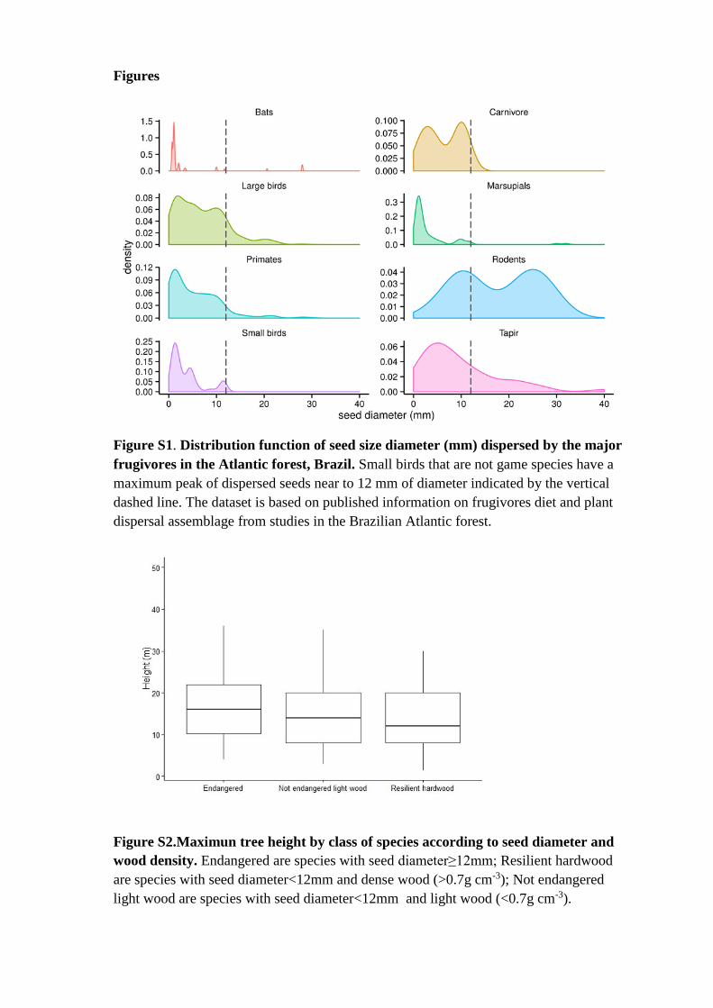
Figure S1. Distribution function of seed size diameter (mm) dispersed by the major
frugivores in the Atlantic forest, Brazil. Small birds that are not game species have a
maximum peak of dispersed seeds near to 12 mm of diameter indicated by the vertical
dashed line. The dataset is based on published information on frugivores diet and plant
dispersal assemblage from studies in the Brazilian Atlantic forest.
Figure S2.Maximun tree height by class of species according to seed diameter and
wood density. Endangered are species with seed diameter≥12mm; Resilient hardwood
are species with seed diameter<12mm and dense wood (>0.7g cm-3); Not endangered
light wood are species with seed diameter<12mm and light wood (<0.7g cm-3).
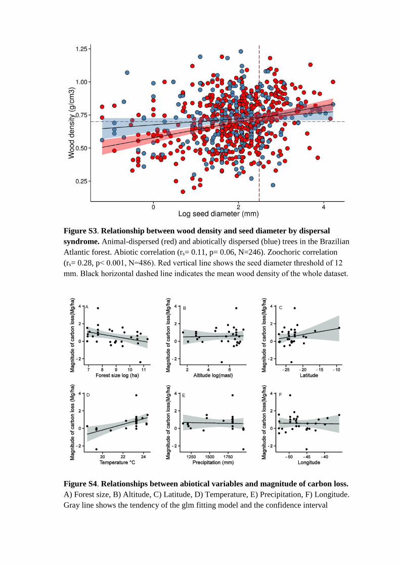
Figure S3. Relationship between wood density and seed diameter by dispersal
syndrome. Animal-dispersed (red) and abiotically dispersed (blue) trees in the Brazilian
Atlantic forest. Abiotic correlation (rs= 0.11, p= 0.06, N=246). Zoochoric correlation
(rs= 0.28, p< 0.001, N=486). Red vertical line shows the seed diameter threshold of 12
mm. Black horizontal dashed line indicates the mean wood density of the whole dataset.
Figure S4. Relationships between abiotical variables and magnitude of carbon loss.
A) Forest size, B) Altitude, C) Latitude, D) Temperature, E) Precipitation, F) Longitude.
Gray line shows the tendency of the glm fitting model and the confidence interval
A B C
D E F
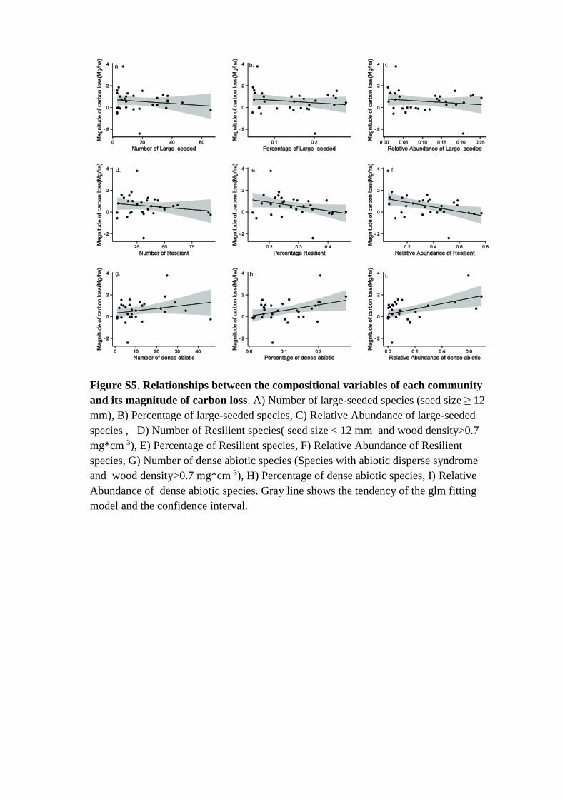
Figure S5. Relationships between the compositional variables of each community
and its magnitude of carbon loss. A) Number of large-seeded species (seed size ≥ 12
mm), B) Percentage of large-seeded species, C) Relative Abundance of large-seeded
species , D) Number of Resilient species( seed size < 12 mm and wood density>0.7
mg*cm-3), E) Percentage of Resilient species, F) Relative Abundance of Resilient
species, G) Number of dense abiotic species (Species with abiotic disperse syndrome
and wood density>0.7 mg*cm-3), H) Percentage of dense abiotic species, I) Relative
Abundance of dense abiotic species. Gray line shows the tendency of the glm fitting
model and the confidence interval.
a. b. c.
d. e. f.
g. h. i.
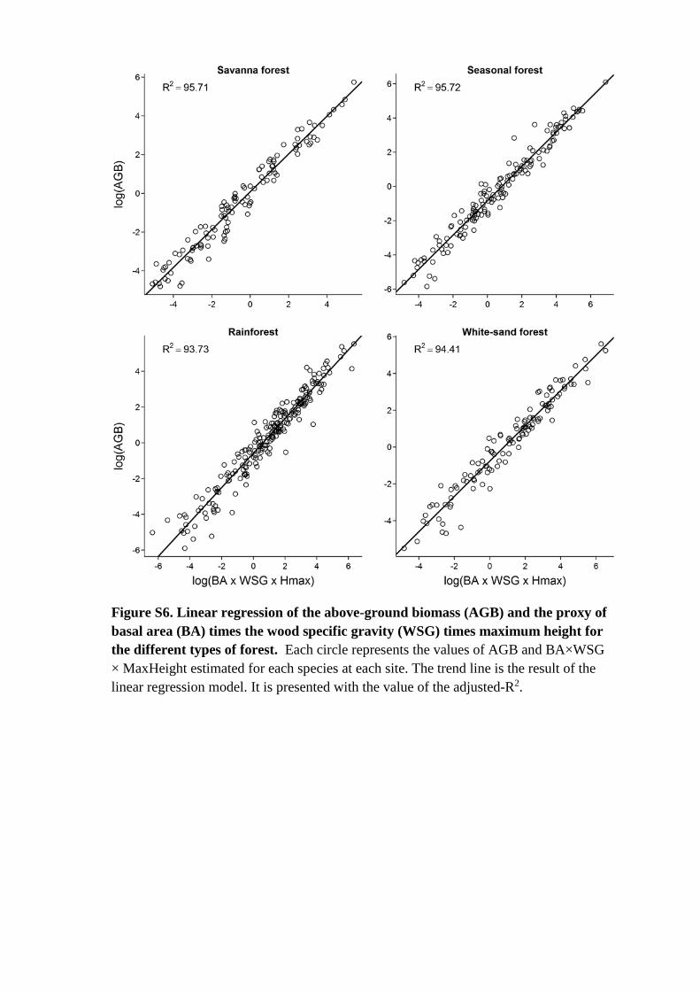
Figure S6. Linear regression of the above-ground biomass (AGB) and the proxy of
basal area (BA) times the wood specific gravity (WSG) times maximum height for
the different types of forest. Each circle represents the values of AGB and BA×WSG
× MaxHeight estimated for each species at each site. The trend line is the result of the
linear regression model. It is presented with the value of the adjusted-R2.
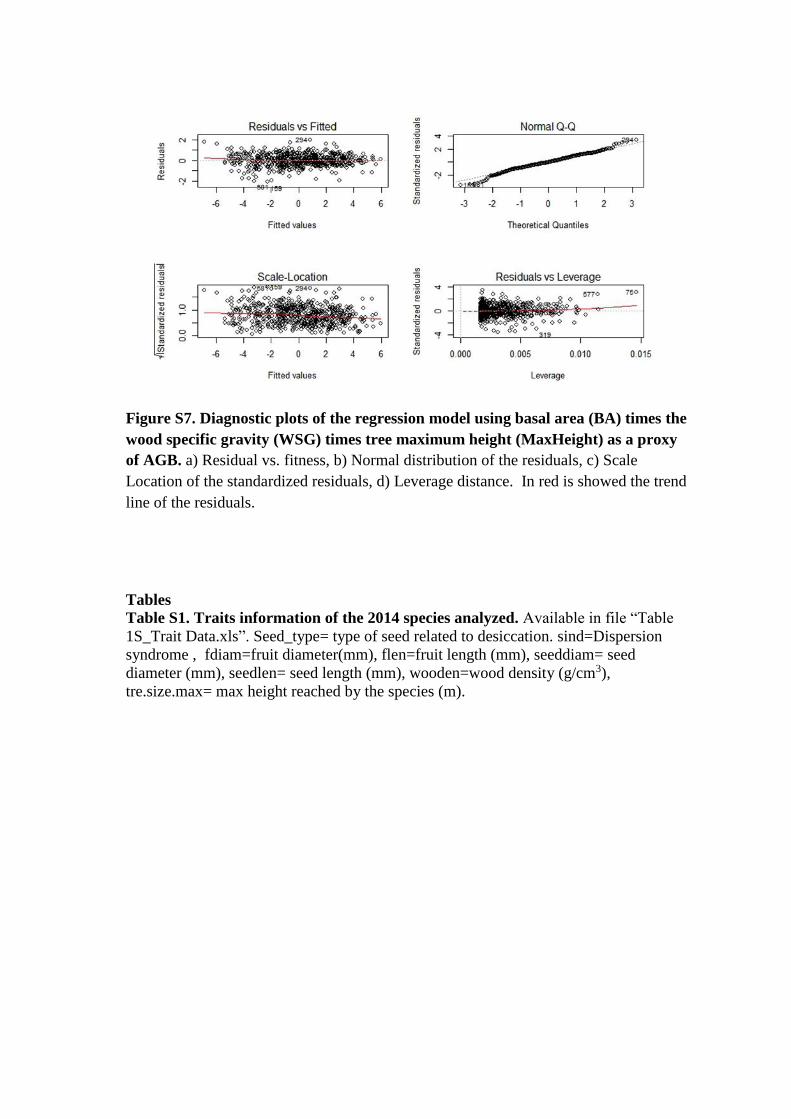
Figure S7. Diagnostic plots of the regression model using basal area (BA) times the
wood specific gravity (WSG) times tree maximum height (MaxHeight) as a proxy
of AGB. a) Residual vs. fitness, b) Normal distribution of the residuals, c) Scale
Location of the standardized residuals, d) Leverage distance. In red is showed the trend
line of the residuals.
Tables Table S1. Traits information of the 2014 species analyzed. Available in file “Table
1S_Trait Data.xls”. Seed_type= type of seed related to desiccation. sind=Dispersion
syndrome , fdiam=fruit diameter(mm), flen=fruit length (mm), seeddiam= seed
diameter (mm), seedlen= seed length (mm), wooden=wood density (g/cm3),
tre.size.max= max height reached by the species (m).
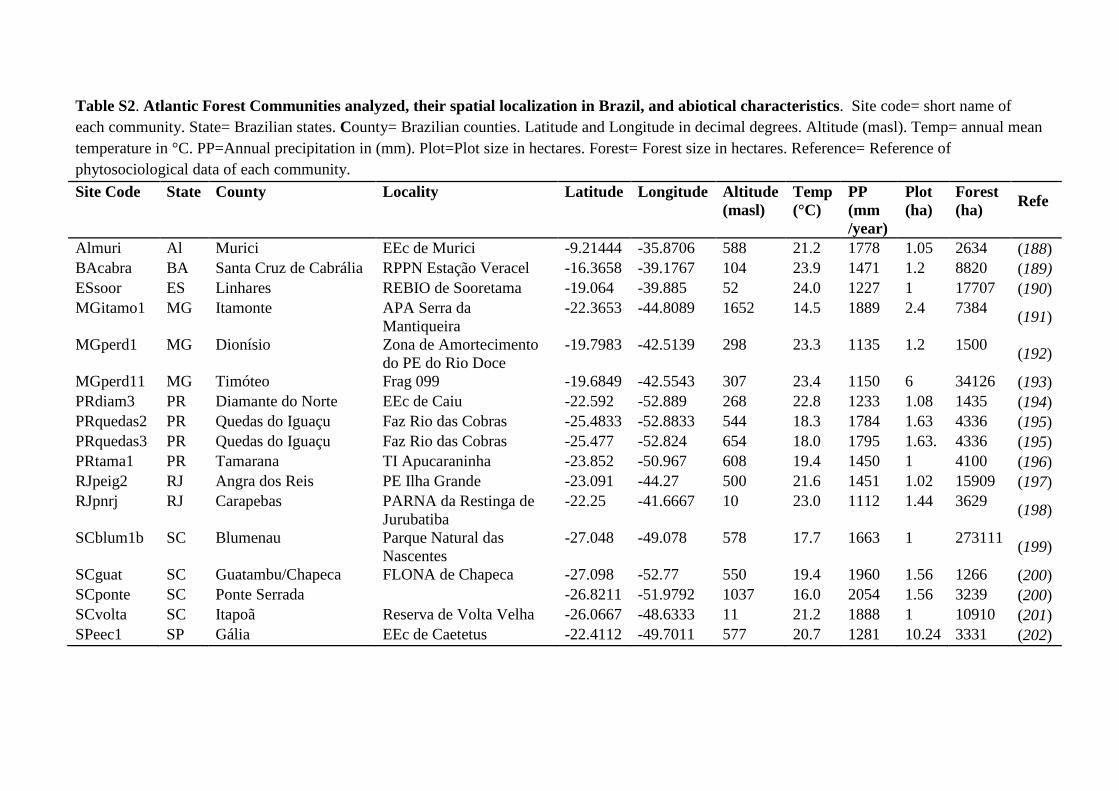
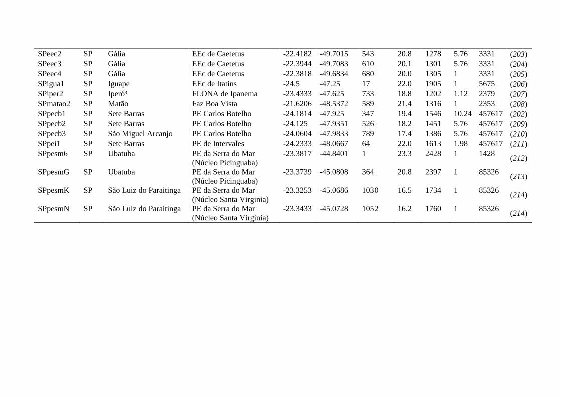
Table S2. Atlantic Forest Communities analyzed, their spatial localization in Brazil, and abiotical characteristics. Site code= short name of
each community. State= Brazilian states. County= Brazilian counties. Latitude and Longitude in decimal degrees. Altitude (masl). Temp= annual mean
temperature in °C. PP=Annual precipitation in (mm). Plot=Plot size in hectares. Forest= Forest size in hectares. Reference= Reference of
phytosociological data of each community.
Site Code State County Locality Latitude Longitude Altitude
(masl)
Temp
(°C)
PP
(mm
/year)
Plot
(ha)
Forest
(ha) Refe
rence
Almuri Al Murici EEc de Murici -9.21444 -35.8706 588 21.2 1778 1.05 2634 (188)
BAcabra BA Santa Cruz de Cabrália RPPN Estação Veracel -16.3658 -39.1767 104 23.9 1471 1.2 8820 (189)
ESsoor ES Linhares REBIO de Sooretama -19.064 -39.885 52 24.0 1227 1 17707 (190)
MGitamo1 MG Itamonte APA Serra da
Mantiqueira
-22.3653 -44.8089 1652 14.5 1889 2.4 7384 (191)
MGperd1 MG Dionísio Zona de Amortecimento
do PE do Rio Doce
-19.7983 -42.5139 298 23.3 1135 1.2 1500 (192)
MGperd11 MG Timóteo Frag 099 -19.6849 -42.5543 307 23.4 1150 6 34126 (193)
PRdiam3 PR Diamante do Norte EEc de Caiu -22.592 -52.889 268 22.8 1233 1.08 1435 (194)
PRquedas2 PR Quedas do Iguaçu Faz Rio das Cobras -25.4833 -52.8833 544 18.3 1784 1.63 4336 (195)
PRquedas3 PR Quedas do Iguaçu Faz Rio das Cobras -25.477 -52.824 654 18.0 1795 1.63. 4336 (195)
PRtama1 PR Tamarana TI Apucaraninha -23.852 -50.967 608 19.4 1450 1 4100 (196)
RJpeig2 RJ Angra dos Reis PE Ilha Grande -23.091 -44.27 500 21.6 1451 1.02 15909 (197)
RJpnrj RJ Carapebas PARNA da Restinga de
Jurubatiba
-22.25 -41.6667 10 23.0 1112 1.44 3629 (198)
SCblum1b SC Blumenau Parque Natural das
Nascentes
-27.048 -49.078 578 17.7 1663 1 273111 (199)
SCguat SC Guatambu/Chapeca FLONA de Chapeca -27.098 -52.77 550 19.4 1960 1.56 1266 (200)
SCponte SC Ponte Serrada -26.8211 -51.9792 1037 16.0 2054 1.56 3239 (200)
SCvolta SC Itapoã Reserva de Volta Velha -26.0667 -48.6333 11 21.2 1888 1 10910 (201)
SPeec1 SP Gália EEc de Caetetus -22.4112 -49.7011 577 20.7 1281 10.24 3331 (202)
SPeec2 SP Gália EEc de Caetetus -22.4182 -49.7015 543 20.8 1278 5.76 3331 (203)
SPeec3 SP Gália EEc de Caetetus -22.3944 -49.7083 610 20.1 1301 5.76 3331 (204)
SPeec4 SP Gália EEc de Caetetus -22.3818 -49.6834 680 20.0 1305 1 3331 (205)
SPigua1 SP Iguape EEc de Itatins -24.5 -47.25 17 22.0 1905 1 5675 (206)
SPiper2 SP Iperó³ FLONA de Ipanema -23.4333 -47.625 733 18.8 1202 1.12 2379 (207)
SPmatao2 SP Matão Faz Boa Vista -21.6206 -48.5372 589 21.4 1316 1 2353 (208)
SPpecb1 SP Sete Barras PE Carlos Botelho -24.1814 -47.925 347 19.4 1546 10.24 457617 (202)
SPpecb2 SP Sete Barras PE Carlos Botelho -24.125 -47.9351 526 18.2 1451 5.76 457617 (209)
SPpecb3 SP São Miguel Arcanjo PE Carlos Botelho -24.0604 -47.9833 789 17.4 1386 5.76 457617 (210)
SPpei1 SP Sete Barras PE de Intervales -24.2333 -48.0667 64 22.0 1613 1.98 457617 (211)
SPpesm6 SP Ubatuba PE da Serra do Mar
(Núcleo Picinguaba)
-23.3817 -44.8401 1 23.3 2428 1 1428 (212)
SPpesmG SP Ubatuba PE da Serra do Mar
(Núcleo Picinguaba)
-23.3739 -45.0808 364 20.8 2397 1 85326 (213)
SPpesmK SP São Luiz do Paraitinga PE da Serra do Mar
(Núcleo Santa Virginia)
-23.3253 -45.0686 1030 16.5 1734 1 85326 (214)
SPpesmN SP São Luiz do Paraitinga PE da Serra do Mar
(Núcleo Santa Virginia)
-23.3433 -45.0728 1052 16.2 1760 1 85326 (214)
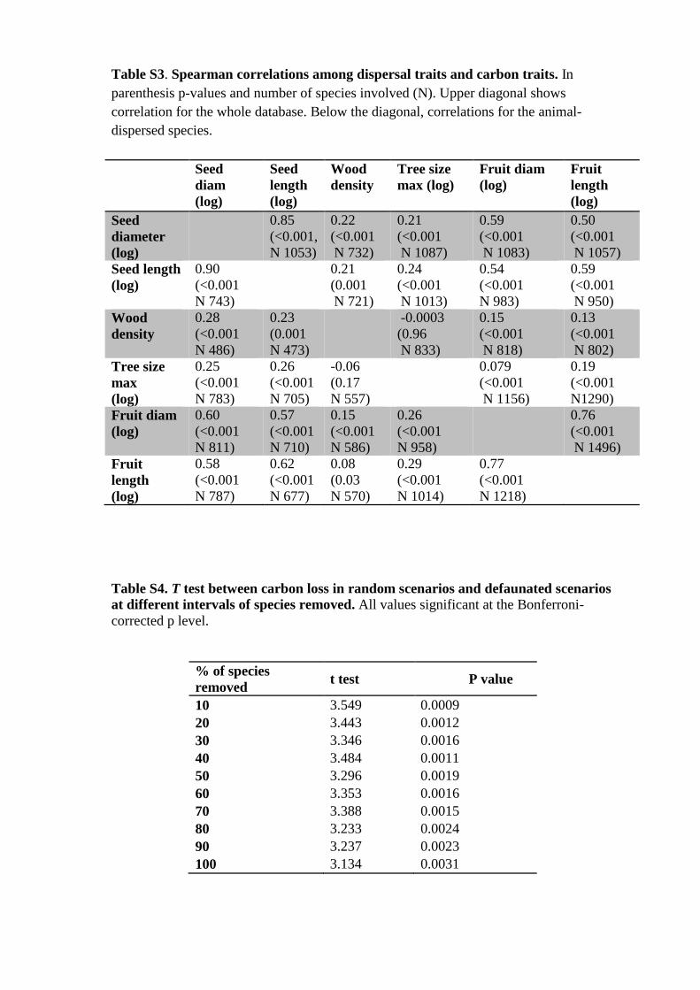
Table S3. Spearman correlations among dispersal traits and carbon traits. In
parenthesis p-values and number of species involved (N). Upper diagonal shows
correlation for the whole database. Below the diagonal, correlations for the animal-
dispersed species.
Seed
diam
(log)
Seed
length
(log)
Wood
density
Tree size
max (log)
Fruit diam
(log)
Fruit
length
(log)
Seed
diameter
(log)
0.85
(<0.001,
N 1053)
0.22
(<0.001
N 732)
0.21
(<0.001
N 1087)
0.59
(<0.001
N 1083)
0.50
(<0.001
N 1057)
Seed length
(log)
0.90
(<0.001
N 743)
0.21
(0.001
N 721)
0.24
(<0.001
N 1013)
0.54
(<0.001
N 983)
0.59
(<0.001
N 950)
Wood
density
0.28
(<0.001
N 486)
0.23
(0.001
N 473)
-0.0003
(0.96
N 833)
0.15
(<0.001
N 818)
0.13
(<0.001
N 802)
Tree size
max
(log)
0.25
(<0.001
N 783)
0.26
(<0.001
N 705)
-0.06
(0.17
N 557)
0.079
(<0.001
N 1156)
0.19
(<0.001
N1290)
Fruit diam
(log)
0.60
(<0.001
N 811)
0.57
(<0.001
N 710)
0.15
(<0.001
N 586)
0.26
(<0.001
N 958)
0.76
(<0.001
N 1496)
Fruit
length
(log)
0.58
(<0.001
N 787)
0.62
(<0.001
N 677)
0.08
(0.03
N 570)
0.29
(<0.001
N 1014)
0.77
(<0.001
N 1218)
Table S4. T test between carbon loss in random scenarios and defaunated scenarios
at different intervals of species removed. All values significant at the Bonferroni-
corrected p level.
% of species
removed t test P value
10 3.549 0.0009
20 3.443 0.0012
30 3.346 0.0016
40 3.484 0.0011
50 3.296 0.0019
60 3.353 0.0016
70 3.388 0.0015
80 3.233 0.0024
90 3.237 0.0023
100 3.134 0.0031
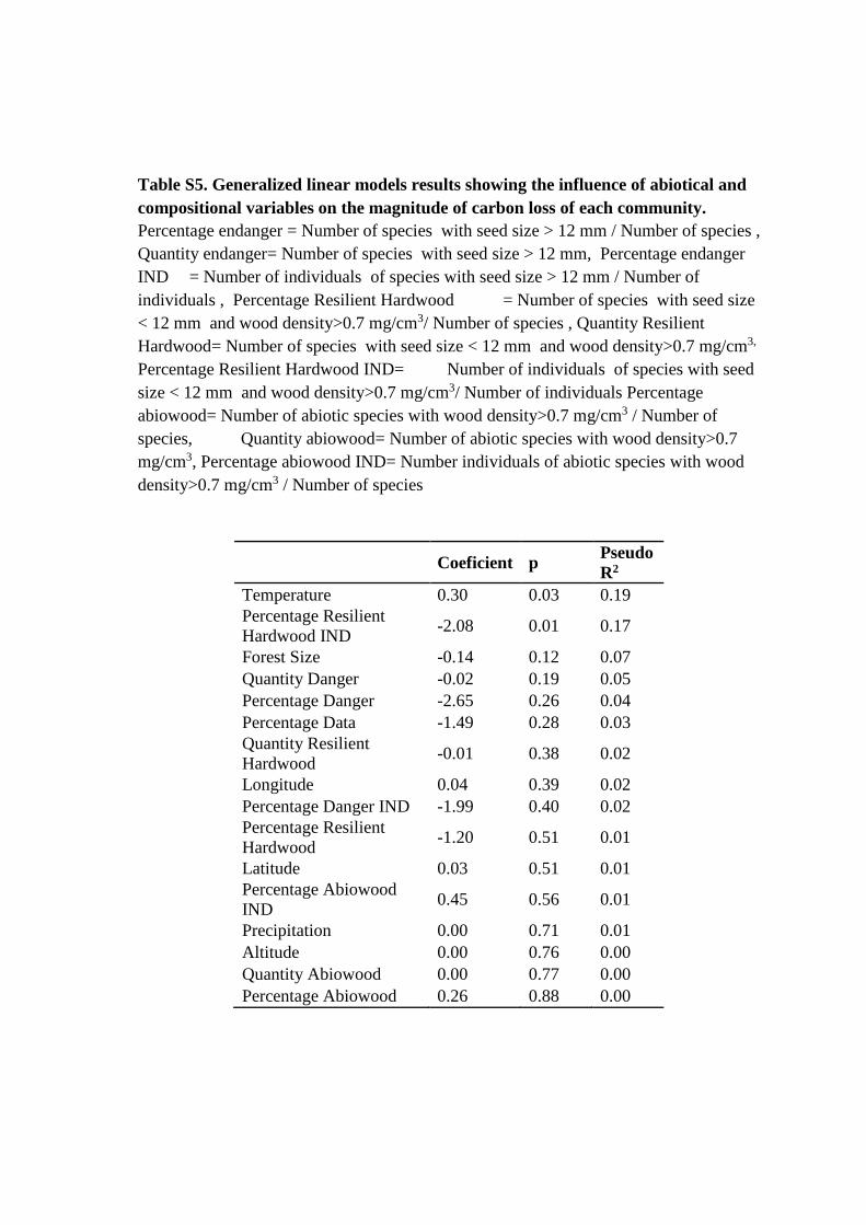
Table S5. Generalized linear models results showing the influence of abiotical and
compositional variables on the magnitude of carbon loss of each community.
Percentage endanger = Number of species with seed size > 12 mm / Number of species ,
Quantity endanger= Number of species with seed size > 12 mm, Percentage endanger
IND = Number of individuals of species with seed size > 12 mm / Number of
individuals , Percentage Resilient Hardwood = Number of species with seed size
< 12 mm and wood density>0.7 mg/cm3/ Number of species , Quantity Resilient
Hardwood= Number of species with seed size < 12 mm and wood density>0.7 mg/cm3,
Percentage Resilient Hardwood IND= Number of individuals of species with seed
size < 12 mm and wood density>0.7 mg/cm3/ Number of individuals Percentage
abiowood= Number of abiotic species with wood density>0.7 mg/cm3 / Number of
species, Quantity abiowood= Number of abiotic species with wood density>0.7
mg/cm3, Percentage abiowood IND= Number individuals of abiotic species with wood
density>0.7 mg/cm3 / Number of species
Coeficient p
Pseudo
R2
Temperature 0.30 0.03 0.19
Percentage Resilient
Hardwood IND -2.08 0.01 0.17
Forest Size -0.14 0.12 0.07
Quantity Danger -0.02 0.19 0.05
Percentage Danger -2.65 0.26 0.04
Percentage Data -1.49 0.28 0.03
Quantity Resilient
Hardwood -0.01 0.38 0.02
Longitude 0.04 0.39 0.02
Percentage Danger IND -1.99 0.40 0.02
Percentage Resilient
Hardwood -1.20 0.51 0.01
Latitude 0.03 0.51 0.01
Percentage Abiowood
IND 0.45 0.56 0.01
Precipitation 0.00 0.71 0.01
Altitude 0.00 0.76 0.00
Quantity Abiowood 0.00 0.77 0.00
Percentage Abiowood 0.26 0.88 0.00
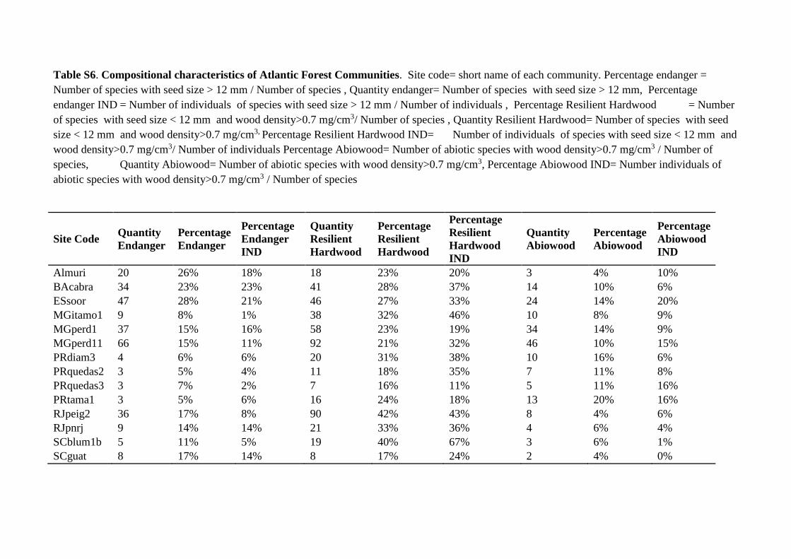
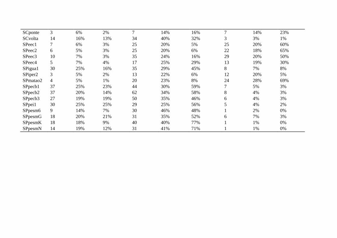
Table S6. Compositional characteristics of Atlantic Forest Communities. Site code= short name of each community. Percentage endanger =
Number of species with seed size > 12 mm / Number of species , Quantity endanger= Number of species with seed size > 12 mm, Percentage
endanger IND = Number of individuals of species with seed size > 12 mm / Number of individuals , Percentage Resilient Hardwood = Number
of species with seed size < 12 mm and wood density>0.7 mg/cm3/ Number of species , Quantity Resilient Hardwood= Number of species with seed
size < 12 mm and wood density>0.7 mg/cm3, Percentage Resilient Hardwood IND= Number of individuals of species with seed size < 12 mm and
wood density>0.7 mg/cm3/ Number of individuals Percentage Abiowood= Number of abiotic species with wood density>0.7 mg/cm3 / Number of
species, Quantity Abiowood= Number of abiotic species with wood density>0.7 mg/cm3, Percentage Abiowood IND= Number individuals of
abiotic species with wood density>0.7 mg/cm3 / Number of species
Site Code Quantity
Endanger
Percentage
Endanger
Percentage
Endanger
IND
Quantity
Resilient
Hardwood
Percentage
Resilient
Hardwood
Percentage
Resilient
Hardwood
IND
Quantity
Abiowood
Percentage
Abiowood
Percentage
Abiowood
IND
Almuri 20 26% 18% 18 23% 20% 3 4% 10%
BAcabra 34 23% 23% 41 28% 37% 14 10% 6%
ESsoor 47 28% 21% 46 27% 33% 24 14% 20%
MGitamo1 9 8% 1% 38 32% 46% 10 8% 9%
MGperd1 37 15% 16% 58 23% 19% 34 14% 9%
MGperd11 66 15% 11% 92 21% 32% 46 10% 15%
PRdiam3 4 6% 6% 20 31% 38% 10 16% 6%
PRquedas2 3 5% 4% 11 18% 35% 7 11% 8%
PRquedas3 3 7% 2% 7 16% 11% 5 11% 16%
PRtama1 3 5% 6% 16 24% 18% 13 20% 16%
RJpeig2 36 17% 8% 90 42% 43% 8 4% 6%
RJpnrj 9 14% 14% 21 33% 36% 4 6% 4%
SCblum1b 5 11% 5% 19 40% 67% 3 6% 1%
SCguat 8 17% 14% 8 17% 24% 2 4% 0%
SCponte 3 6% 2% 7 14% 16% 7 14% 23%
SCvolta 14 16% 13% 34 40% 32% 3 3% 1%
SPeec1 7 6% 3% 25 20% 5% 25 20% 60%
SPeec2 6 5% 3% 25 20% 6% 22 18% 65%
SPeec3 10 7% 3% 35 24% 16% 29 20% 50%
SPeec4 5 7% 4% 17 25% 29% 13 19% 30%
SPigua1 30 25% 16% 35 29% 45% 8 7% 8%
SPiper2 3 5% 2% 13 22% 6% 12 20% 5%
SPmatao2 4 5% 1% 20 23% 8% 24 28% 69%
SPpecb1 37 25% 23% 44 30% 59% 7 5% 3%
SPpecb2 37 20% 14% 62 34% 58% 8 4% 3%
SPpecb3 27 19% 19% 50 35% 46% 6 4% 3%
SPpei1 30 25% 25% 29 25% 56% 5 4% 2%
SPpesm6 9 14% 7% 30 46% 48% 1 2% 0%
SPpesmG 18 20% 21% 31 35% 52% 6 7% 3%
SPpesmK 18 18% 9% 40 40% 77% 1 1% 0%
SPpesmN 14 19% 12% 31 41% 71% 1 1% 0%