www.sciencemag.org/cgi/content/full/science.1233137/DC1

Supplementary Materials for

Pliocene Warmth, Polar Amplification, and Stepped Pleistocene Cooling Recorded in NE Arctic Russia

Julie Brigham-Grette,* Martin Melles, Pavel Minyuk, Andrei Andreev, Pavel Tarasov, Robert DeConto, Sebastian Koenig, Norbert Nowaczyk, Volker Wennrich, Peter Rosén,

Eeva Haltia, Tim Cook, Catalina Gebhardt, Carsten Meyer-Jacob, Jeff Snyder, Ulrike Herzschuh

*Corresponding author. E-mail: juliebg@geo.umass.edu

Published 9 May 2013 on Science Express

DOI: 10.1126/science.1233137

This PDF file includes:

Materials and Methods SupplementaryText Figs. S1 to S9 Tables S1 to S5 References (64–105)

2

Materials and Methods Drilling and Creation of Composite Record

Lake El’gygytgyn was initially investigated based on pilot percussion cores (PG1351 and PG1352) representing the paleoclimate history of the lake back in time to 250 ka (64, and papers there in). Scientific drilling at Lake El’gygytgyn later took place over the winter and spring of 2008/2009 in central Chukotka, northeastern Russia (cf. Fig.1). First a single borehole was drilled in permafrost outside the lake talik to a depth of 141 m (5011-3) and later three adjacent drill cores (5011-1, A, B and C) were taken from near the center of the lake (28) as summarized in Table S1. With casing set into the uppermost lake sediments, drilling recovery began at a depth of ~5.66 m near the base of the last interglacial (MIS 5e). The uppermost part of the core was spliced with percussion core Lz1024 taken in 2003 (16 m in length, with a basal age of 300 ka; 27), to create a continuous composite record.

Table S1. Penetration, drilling and core recovery at ICDP Sites 5011-1 and 5011-3 in the El´gygytgyn Crater (all data given in field depth; mblf = meters below lake floor).

Site Hole Type of Material Penetrated (mblf)

Drilled (m)

Recovered (m)

Recovery (%)

5011-1 1A lake sediment 146.6 143.7 132.0 92 1B lake sediment 111.9 108.4 106.6 98 1C total 517.3 431.5 273.8 63 lake sediment 225.3 116.1 52 impact rocks 207.5 157.4 76

5011-3 permafrost deposits 141.5 141.5 129.9 91

Where replicate cores were available, the composite profile for ICDP Site 5011-1 (given in corrected depths below lake floor (blf)) was constructed from the best-preserved sediment intervals in overlapping core sequences (Table S1), based upon visual core inspection supported by variations in proxy data. Volcanic ash layers and mass movement events in Lake El´gygytgyn, like those investigated in detail for the last three glacial/interglacial cycles (65), were generally omitted if their thicknesses exceeded 5 cm, producing small gaps within the composite proxy data sets. Below 5.66 m to a depth of 104.8 m blf, alternating sediment intervals from parallel cores 5011-1A and -1B were spliced together. Between 104.8 m and 145.7 m blf, cores 1A, 1B and 1C contributed to the composite. Below 145.7 m, down to the sediment-impact breccia interface at 318 m blf composite depth, the record relies solely on core 5011-1C. The largest gap in recovery in core 5011-1C occurs from 150.074 to 159.524 m representing the time interval from 2977.2 to 3032.6 ka.

Sediment Facies

The characteristics of pelagic sediments in Lake El’gygytgyn are highly variable (Fig. S1). A combination of physical characteristics, including color, particle size, and the presence or absence of various sedimentary structures was used to define distinct lithofacies. These distinctions were based primarily on visual inspection of split core

3

halves and high-resolution (200 µm) radiographs supplemented by quantitative particle-size analysis and the interpretation of thin-sections prepared from epoxy-impregnated sediment slabs obtained from selected regions of the core.

Fig. S1. Line scan images of the primary lithofacies identified in the lacustrine sequence from Lake El’gygytgyn. Facies A is limited to the Pleistocene interval of the core whereas Facies D and E are found only in the Pliocene section; Facies B and C are found throughout the record. The gap in the image of Facies E is included to highlight two sections of brecciated sediment, however the total interval depicted represents a continuous sequence.

Three distinct lithofacies (Facies A, B, and C) dominate the pelagic sediments of

the Pleistocene portion of the Lake El’gygytgyn record and have been described previously (18, 27, 66). Facies A consists of dark gray to black, sub-millimeter, clastic laminations (silt and clay) and was previously linked with pronounced glacial/stadial conditions and the presence of perennial lake-ice cover. Facies B, the most abundant pelagic facies is variably olive-gray to brown, composed of massive to faintly banded silt, and lacks distinct sedimentary structures. Facies B is interpreted as representing the predominant, albeit widely varying Quaternary climate and environmental conditions at Lake El’gygytgyn. Facies C is defined by a distinct reddish brown appearance and the presence of faint pale white, millimeter to centimeter scale laminations. This facies is always traced back to an exceptionally warm interglacial climate.

Throughout the Pliocene portion of the record Facies B and C continue to occur as the most dominant pelagic facies while Facies A is not observed. However, due to gaps in core recovery (Fig. S2) it cannot be stated unequivocally that Facies A does not occur in the Pliocene section. Nonetheless two additional facies (Facies D and E) not

4

observed in upper portions of the record are exclusively observed within the Pliocene section of the record.

Facies D is similar to the clastic laminated Facies A found in the younger part of the record but is distinguished by the significantly larger average thickness of the laminae which range up to ~1 cm in thickness and average several millimeters. Laminations have distinct lower bounding surfaces and grade upwards from silt to clay before repeating. Facies D is predominantly gray in color, however the earliest occurrences of the unit are more variable in color including both red and green hues. Median particle size ranges from approximately 2 to 6 µm with clay-sized particles comprising 40 to 60 % of the sediment. For a given median particle size Facies D is composed of a higher clay content than other lithofacies, particularly in comparison with the laminated units found in the younger part of the record (Facies A), which typically contain less than 30 % clay-sized particles. The well-preserved laminations in Facies D indicate a lack of physical disturbance of bottom sediments either through bioturbation or density-driven or wind-induced circulation of bottom waters. Repeated deposition of graded silt and clay laminations suggests repeated pulses of sediment delivery to the lake due to variations in fluvial input and stream competency. The higher mean thickness and higher clay content of Facies D relative to later laminated deposits (Facies A and C) are consistent with more rapid weathering and delivery of sediment to the lake during the Pliocene. This interpretation is supported by a higher overall sediment accumulation rate during the Pliocene as indicated by the age-depth relationship of the record (Figs. S3 to S5).

Fig. S2. Magnetic susceptibility (red: core data; blue: downhole logging data) and lithological facies against depth. Pleistocene laminated Facies A is shown in turquoise and blue, homogeneous Facies B in ochre, super interglacial Facies C in red, Pliocene laminated Facies D in lilac, and transitional Facies E in grey. Mass movement deposits are marked as Facies F with turbidites in orange and all other mass movement deposits (slides, slumps, debrites and grain flow deposits) in green. Minor core gaps occur where there are not colors in any column.

5

Facies E is composed of gray to reddish-brown clay, silt and fine sand in thin to medium thick beds (Fig. S1). The defining characteristic of Facies E is the presence of intermittent brecciated intervals. Brecciated intervals range from a few centimeters up to 10 cm in thickness and typically occur at transitions in grain size spaced tens of cm apart. Individual clasts are angular, finer in grain size (clay sized particles) relative to the surrounding matrix, and are generally cm sized or smaller. Clasts appear similar in nature to the underlying sediment and with an absence of rounding; they are interpreted as having likely formed in place. These brecciated intervals may have resulted from dewatering associated with additional sediment loading or may indicate brief intervals of desiccation. Facies E immediately overlies impact breccia and suevite associated with the meteorite impact that formed Lake El’gygytgyn and is thus interpreted as a transitional facies representing processes during lake filling and onset of the first lacustrine deposition in the impact crater.

Fig. S3. Sedimentation rates from ICDP Site 5011-1 (center), according to the age model shown in Figure S5 together with the marine benthic oxygen isotope stack LR04 (21; top) and the obtained polarity pattern for the time interval from 2500 to 3600 ka. Black dashed lines indicate polarity reversals identified in ICDP Site 5011-1 cores (bottom). Black (gray) indicates normal polarity, white indicates reversed polarity. The vertical dashed red arrow marks the time of the impact that created the depression filled by Lake El'gygytgyn at 3.58±0.04 Ma (17).

6

Fig. S4. Tuning of Pliocene sediments from ICDP Site 5011-1, Lake El'gygytgyn, Far East Russian Arctic: (A) percentage of tree and shrub pollen, (B) marine benthic oxygen isotope stack LR04 (21) with labels for the major marine isotope stages (101 to MG8), (C) biogenic versus lithogenic input, estimated by the Si/Ti ratio from XRF (X-ray fluorescence) scanning in counts, (D) percentage of biogenic silica (BSi) derived from Fourier Transform Infrared Spectroscopy (FTIRS), (E) amount of total organic carbon (TOC), (F) geomagnetic polarity time scale, with black (white) bars denoting normal (reversed) polarity. The red dotted line marks the time of the impact at 3.58±0.04 Ma (17). Black dashed lines indicate polarity reversals identified in ICDP Site 5011-1 core, orange (green) dashed lines indicate correlation of FTIRS-BSi, Si/Ti-ratio, and TOC (tree pollen) to the LR04 stack. Age Model

The age model for the ICDP Site 5011-1 sedimentary composite record was developed in several steps, successively refining the model (see 19, supplementary materials). Continuous sampling of available core material was performed using U-channels mostly in the upper ~150 m blf. Below that depth, preferably discrete samples (n=446, volume ca. 6 cm3) at ca. 10 cm intervals were taken, where consolidation of the sediments exceeded a certain workable degree, inhibiting the extraction of U-channels.

7

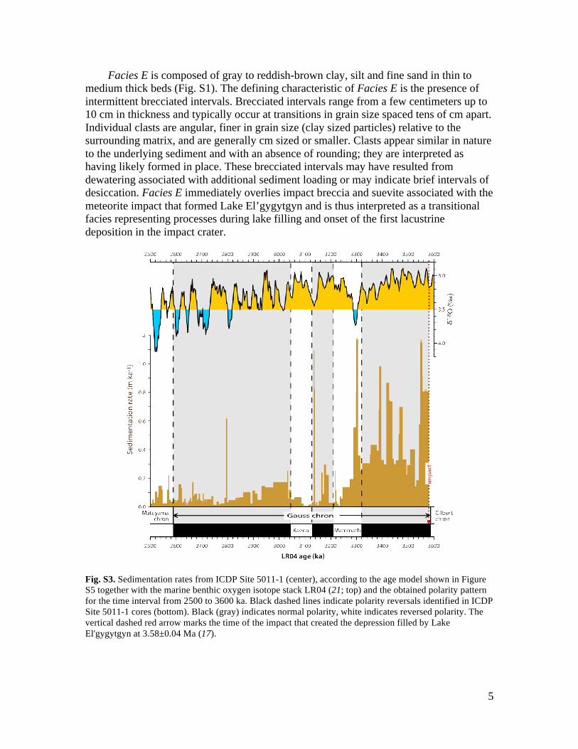
Stepwise alternating field demagnetization of all sampled material in ten steps of up to 100 mT peak amplitude and subsequently applied principle component analysis of the obtained data sets defined the position of major reversals in the Pliocene including the Matuyama/Gauss boundary and the intra-Gauss reversals of the Kaena and Mammoth subchrons (black dashed lines, Fig. S4). The age of the El'gygytgyn impact at 3.58±0.04 Ma (17) provided another initial tie point (red dotted line in Fig. S4). Since the lowermost sediments exhibit a clear normal polarity, the impact definitely occurred after the Gauss/Gilbert boundary, dated at 3.58 Ma (21).

Fig. S5. Age/depth model of (18) for the core composite at ICDP Site 5011-1 in Lake El’gygytgyn, based on magnetostratigraphy as well as correlations between proxy data, the LR04 marine stack (21) and insolation. Black diamonds are first order tie points; second and third order tie points in blue line. The red star marks the dated time of impact at 3.58 (±0.04) Ma (17). Normal (black) and reversed (white) polarities are shown on the left side. Mass movement events (gray) and core gaps (blue) larger than 50 cm thickness are shown on the right side.

8

Additional tie points could be derived from climatically controlled sedimentological parameters such as biogenic silica (BSi), determined by Fourier Transform Infrared Spectroscopy (FTIRS), and the Si/Ti ratio obtained from high-resolution X-ray fluorescence (XRF) scanning, which both reflect the primary bio-production, that is, the abundance of diatoms. Since Si comprises input from both biogenic silica and lithogenic silica, whereas Ti only reflects lithogenic input to the lake sediments, the Si/Ti ratio reflects, as a first approximation, variations in biogenic productivity (diatom blooms) versus the clastic background sedimentation. Analyzing Si/Ti data obtained around the documented reversals shows that diatom production, and also the amount of total organic carbon (TOC), is high in warm stages and low in cold stages throughout the Pliocene in ICDP Site 5011-1 sediments (Fig. S4). Thus further tie points were obtained by tuning the Si/Ti ratio, BSi content, as well as TOC content with the LR04 stack (21) back to around 2.9 Ma, equal to marine isotope stages (MIS) 101 to G17 (orange dashed lines in Fig. S4), and between terminations of the Kaena and Mammoth subchrons (~3.20 to ~3.04 Ma).

Due to larger coring gaps, tuning was compromised around 3.24 and 3.0 Ma, respectively. Poor core recovery and numerous mass movement deposits in most of the lower half of ICDP Site 5011-1, equivalent to the time interval from around 3.3 Ma back to the time of the impact at 3.58 Ma, also hampered a straight-forward correlation of proxy-data to the LR04 reference record. Nevertheless, due to the ten-fold higher sedimentation rate even the sporadic sampling of stratigraphic information caused by the poor core recovery provided sufficient data to identify the major cooling and warming events/trends in the corresponding time interval, e.g., MIS M2, MG4, and MG8 (Fig. 2A). Here, especially the record of tree and shrub pollen, representing climatic conditions in the wider catchment area, allowed the definition of various tie points for the age model (green dashed lines in Fig. S4). The link between global climate variability and tree pollen abundance is confirmed in the younger part of the record (~2.8 to ~2.5 Ma), where the age model is constrained by the Matuyama/Gauss reversal and information from other proxy-records (e.g., Si/Ti ratio, and/or BSi). The age-depth plot for core 5011-1 consistent with (18) is shown in Figure S5.

Other Proxy Methods

Proxy methods utilized across the 3.6 to 2.2 Ma portion of the Lake El’gygytgyn sediment record are partly identical to those reported by (18). Magnetic susceptibility served as an important factor in linking the borehole stratigraphy with downhole logging techniques. Magnetic susceptibility was measured both on-site during the drilling campaign using whole-core measurements, and downhole logging methods for core correlations, and off-site in the laboratory using high-resolution measurements on split cores for orbital tuning.

Whole-core measurements of magnetic susceptibility were conducted in the field shortly after core retrieval with a Geotek Multi-Sensor Core Logger (MSCL; Geotek Ltd., UK), using a Bartington MS-2 meter equipped with a loop sensor of 80 mm internal diameter. Data correction was done in respect to the specific core and loop sensor diameters according to the Bartington Manual (67).

Downhole magnetic susceptibility was measured within the borehole for ICDP 5011-1C using a probe manufactured by Antares (Germany). Data were corrected for the

9

two different borehole diameters (124 mm drill bit size down to 274.33 m blf, correction factor = 1.4; 98 mm drill bit size from 274.33 m blf to the end of the hole, correction factor = 1.25). Both data sets are shown in Fig. S2. The data sets differ in amplitudes due to the divergent methods applied in acquiring the measurements; it is not due to the primary paleoclimate signal.

In the laboratory, magnetic (volume) susceptibility (MS) was measured in 1-mm steps on core halves using an automated split-core logger, in order to repeat the on-site measurements (see above) in much higher resolution. Data from core Lz1024 were acquired with a Bartington MS2E spot-reading sensor in combination with a MS2 control unit. MS from ICDP 5011-1 cores were obtained using a Bartington MS2E sensor first attached to a MS2 control unit, which was later replaced by a technically improved MS3 control unit. The response function of the MS2E sensor with respect to a thin magnetic layer is equivalent to a Gaussian curve with a half-width of slightly less than 4 mm. The amplitude resolution of the sensor was 10×10-6 in combination with the MS2 unit and 2×10-6 with the MS3 unit. During data acquisition, blank readings against air were obtained after every 10 measurements in order to correct the data for small shifts in the sensor's background due to temperature drift.

Silicon/titanium (Si/Ti) ratios were determined on core halves and U-channels using an X-ray fluorescence (XRF) core scanner (ITRAX, Cox Ltd., Sweden), equipped with a Mo-tube set to 30 kV and 30 mA. XRF scanning was performed at 2-mm resolution using an integration time step of 10 s per measurement. Because the intensities derived from wet sediments, especially those of light elements such as Si, might be influenced by effects of the sediment matrix (68), matrix-corrected Si counts (Simc) were calculated from the raw Si integrals (Siraw) using the empirically determined formula

€

Simc =Siraw

3.2994 *e−0.505*inc / coh (1)

Eq. (1) is based on an exponential attenuation function between the ratio of wet and

dry element intensities and the ITRAX-derived ratio of Compton and Rayleigh scattering (inc/coh ratio) of 340 samples from the Lake El´gygytgyn record. The inc/coh ratio in general is dependent on the average atomic number of the sample and thus has been used as an indicator for organic matter content and/or matrix-induced density variations (69).

For biogeochemical analyses, one of the core halves was continuously sub-sampled at 2-cm intervals. The samples were freeze-dried and ground to < 63 µm, then biogenic silica (BSi) was quantified every 2 cm using Fourier Transform Infrared Spectroscopy (FTIRS) by Bruker (Ltd.) Ifs 66/v and Vertex 70 spectrometers. Analyses, sample preparation, and calibration of the resulting counts followed the methods described in (70), with the exception that only samples from Lake El’gygytgyn were included in the FTIRS-BSi calibration model.

Calculation of accumulation rates (acc. rate) of BSi required information concerning age and density/porosity for each sample. Density and porosity were determined employing a Geotek MSCL on split cores equipped with a 137Cs gamma ray source. For calibration, standard core-size semi-cylinders consisting of different proportions of aluminum and water were logged according to the method described by (71) but modified for split cores. The thickness of split cores was measured via ITRAX XRF core scanner

10

(ITRAX, Cox Ltd., Sweden) simultaneously along with XRF measurements. These measurements are more accurate than what is possible via the MSCL for split cores of this size. GRAPE density and porosity were then calculated using the method described in the Geotek manual (67). Grain density for the calculation of porosity was calculated using the BSi percentage and a mean grain density of 2.1 g cm-3 for diatomaceous ooze (72) and 2.65 g cm-3 for quartz (67). Density and porosity values were taken from measurements not further away than 10 cm from the actual biogenic silica sample. For each sample, the composite age was calculated using linear interpolation between the tie points of the age model (Fig. S5). Sedimentation rates were calculated between the geomagnetic tie points.

BSi accumulation rates (CAR) were calculated using the following algorithms by (73):

CAR = s*

€

(ρGRAPE −1.025∗Φ)∗C , (2) with s = sedimentation rate (cm/a), ρGRAPE = GRAPE density (g cm-3), φ = porosity,

and C = BSi content. In the lowermost part of the record, at depths >227.29 m blf (~3.4 Ma), BSi measurements were only carried out on core catcher samples every meter. GRAPE densities and porosities could not be determined on the core catcher samples directly; therefore averaged values from the 2 cm above and below the core catcher were used.

Pollen, Biome and Climate Reconstruction

Continuous pollen studies of the ICDP 5011-1 core composite were carried out on sediments deposited between 3.6 and 2.15 Ma ago (Fig. S6). Sample resolution throughout this interval ranged from 0.5 to 7 ka. Pollen sample processing followed standard techniques used for organic-poor sediments (74). Water-free glycerol was used for sample storage and preparation of the microscopic slides. Pollen and spores as well as a number of non-pollen palynomorphs were identified and counted at magnifications of 400x and 1000x, with the aid of published pollen keys and atlases. Tablets containing Lycopodium marker spores were added to the samples to allow for calculation of pollen concentrations (74). If available, at least 250 pollen grains were counted in each sample. In addition to pollen and spores a number of non-pollen palynomorphs such as fungi spores, remains of algae and invertebrate, were also identified and counted when possible. These non-pollen palynomorphs are also valuable indicators of past environments (e.g. 75, and references therein). Especially important indicators are coprophilous fungi spores (primarily Sporormiella, Sordaria and Podospora), inhabiting dung of grazing animals, and thus, indirectly pointing to the presence of grazing animals in the lake vicinity and confirming the presence of open, treeless habitats in the study area.

11

Fig. S6. Simplified pollen, spores, and non-pollen-palynomorphs diagram for the time interval from 3.56 to 2.15 Ma. F - fungi spores, A - algae remains.

12

Climate-Vegetation Modeling Climate simulations of the mid Pliocene use the current (2011) version of the

GENESIS v. 3.0 GCM (76) interactively coupled to the BIOME4 equilibrium vegetation model (77). The model has been tested extensively in present day and paleoclimate scenarios and simulates modern Arctic climate and distributions of potential vegetation close to observations (39). Simulated mean temperature of the warmest month (MTWM) at Lake El’gygytgyn for modern conditions (12ºC) compare favorably with ground observations and reanalysis products (25). As used here, the atmospheric component has 18 vertical layers, a spectral resolution of T31 (~3.75°), and uses an adapted version of the NCAR CCM3 solar and thermal infrared radiation code (78). The model atmosphere is coupled to 2°×2° surface models including a 50-meter slab ocean model with prognostic sea surface temperatures, diffusive heat transport, and dynamic-thermodynamic sea ice. Terrestrial land surface components include multi-layer snow and soil models, and a land-surface-transfer scheme (LSX) that calculates momentum transfer and fluxes of energy and water between the atmosphere and ice, snow, soil surfaces, and upper and lower vegetation canopies. This version of the GCM has a sensitivity to 2×CO2 of 2.9°C, without vegetation, greenhouse gas, or ice sheet feedbacks.

As in (39), potential equilibrium vegetation distributions are predicted by BIOME4. The model predicts the distribution, community structure, and biogeochemistry of 27 biomes using monthly climatologies of temperature, precipitation, and clouds simulated by the GCM. In turn, the simulated vegetation provides the physical land-surface attributes in LSX. In the model, vegetation types in each grid cell are determined by bioclimatic limits at the same level of CO2 in the GCM, according to tolerances of cold, heat, sunshine and moisture. The boundary between boreal forest and tundra (relevant to the region surrounding Lake El’gygytgyn) is a function of net primary productivity (NPP), which under modern conditions is highly correlated with growing degree-days above 0ºC. In both modern-control and paleoclimate simulations (Fig. 4), the vegetation model was run without bias corrections and simulations were run for 50 years to allow equilibration. Pliocene Model Boundary Conditions

Pliocene land surface elevations assume a geography the same as modern, or with the Greenland Ice Sheet removed (Fig. 4). In simulations without a Greenland Ice Sheet, the sub-glacial land surface is isostatically restored to its equilibrated ice-free elevation (39).

CO2 atmospheric mixing ratios are prescribed at 200 ppmv, 300 ppmv, or 400 ppmv to span a range of values representing Pliocene glacial and interglacial conditions (2, 3). Prescribed CO2 in the “preindustrial” control simulation (using modern orbital values and land surface elevations) is 280 ppmv. CH4, and N2O atmospheric mixing ratios are left at preindustrial values in all simulations (801 and 289 ppbv, respectively).

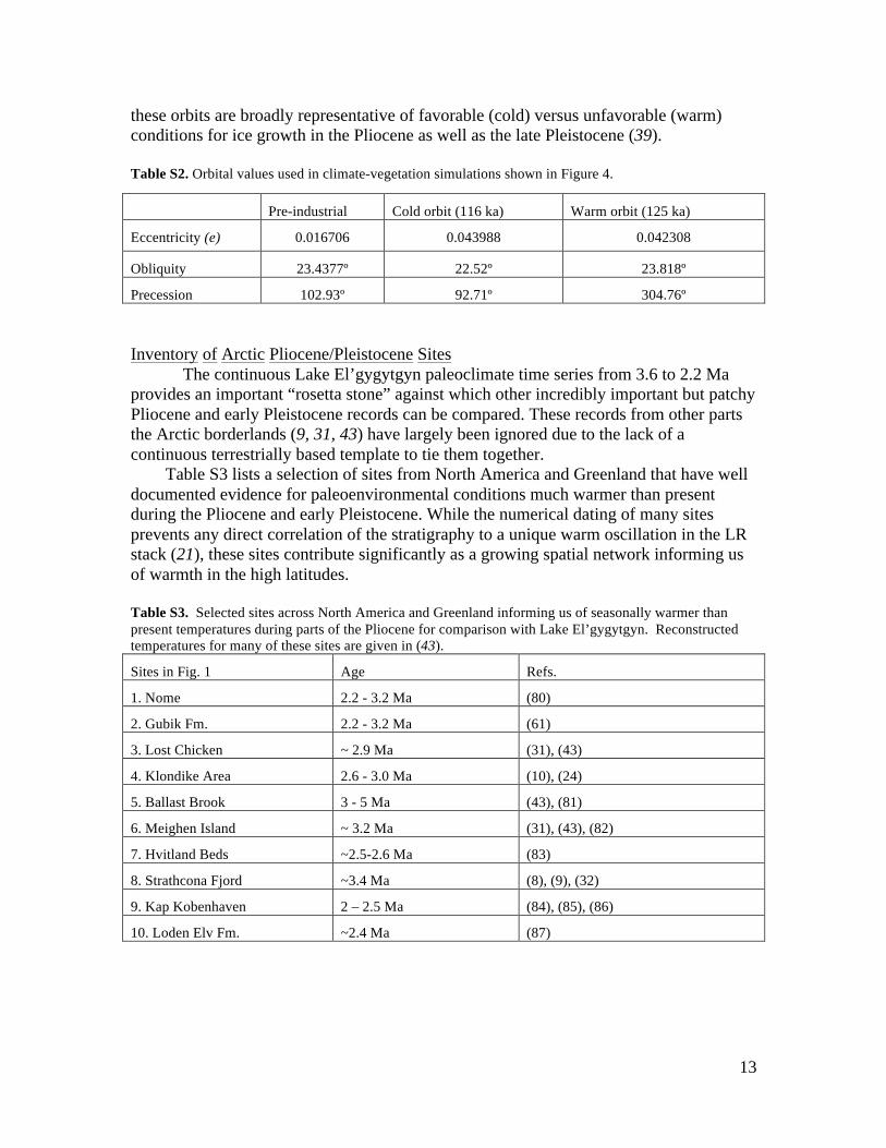
Orbital parameters (Table S2) are varied to represent 1) pre-industrial conditions, 2) cold (glacial) boreal summers, and 3) warm (interglacial) boreal summers. Representative values of orbital eccentricity, obliquity, and the longitude of perihelion (the prograde angle between the vernal equinox and perihelion) are taken from (79) at 116 ka (cold boreal summer orbit) and 125 ka (warm boreal summer orbit), assuming

13

these orbits are broadly representative of favorable (cold) versus unfavorable (warm) conditions for ice growth in the Pliocene as well as the late Pleistocene (39).

Table S2. Orbital values used in climate-vegetation simulations shown in Figure 4.

Pre-industrial Cold orbit (116 ka) Warm orbit (125 ka)

Eccentricity (e) 0.016706 0.043988 0.042308

Obliquity 23.4377º 22.52º 23.818º

Precession 102.93º 92.71º 304.76º

Inventory of Arctic Pliocene/Pleistocene Sites

The continuous Lake El’gygytgyn paleoclimate time series from 3.6 to 2.2 Ma provides an important “rosetta stone” against which other incredibly important but patchy Pliocene and early Pleistocene records can be compared. These records from other parts the Arctic borderlands (9, 31, 43) have largely been ignored due to the lack of a continuous terrestrially based template to tie them together.

Table S3 lists a selection of sites from North America and Greenland that have well documented evidence for paleoenvironmental conditions much warmer than present during the Pliocene and early Pleistocene. While the numerical dating of many sites prevents any direct correlation of the stratigraphy to a unique warm oscillation in the LR stack (21), these sites contribute significantly as a growing spatial network informing us of warmth in the high latitudes.

Table S3. Selected sites across North America and Greenland informing us of seasonally warmer than present temperatures during parts of the Pliocene for comparison with Lake El’gygytgyn. Reconstructed temperatures for many of these sites are given in (43).

Sites in Fig. 1 Age Refs.

1. Nome 2.2 - 3.2 Ma (80)

2. Gubik Fm. 2.2 - 3.2 Ma (61)

3. Lost Chicken ~ 2.9 Ma (31), (43)

4. Klondike Area 2.6 - 3.0 Ma (10), (24)

5. Ballast Brook 3 - 5 Ma (43), (81)

6. Meighen Island ~ 3.2 Ma (31), (43), (82)

7. Hvitland Beds ~2.5-2.6 Ma (83)

8. Strathcona Fjord ~3.4 Ma (8), (9), (32)

9. Kap Kobenhaven 2 – 2.5 Ma (84), (85), (86)

10. Loden Elv Fm. ~2.4 Ma (87)

14

Supplementary Text Additional information on Pollen, Biome and Climate Reconstruction

Vegetation in the area during the earliest history of the lake was first dominated by spruce and pine of the subgenus Haploxylon (e.g., modern Pinus cembra or P. sibirica) with fir, larch, and some hemlock (Tsuga) and Douglas fir (Pseudotsuga) (details in Fig. S6). Pseudotsuga pollen is not distinguishable from Larix (Fig. S7).

Fig. S7. Principle-component analysis of Larix vs. Pseudotsuga before and after the Mammoth Event to test for likely habitat preference.

Hemlock and Douglas fir can tolerate cold and relatively humid conditions but thrive best in relatively moist cool temperate areas with high rainfall, cool summers, and little or no water stress; they are also adapted to cope with severe winter conditions better than most other trees. However, while Larix dominates present-day Siberian light taiga with a high permafrost table and can survive under very cold climate conditions, Pseudotsuga on the other hand, cannot survive in permafrost soils and prefers growth under a temperate climate. The correct interpretation of the Larix/Pseudotsuga pollen record can dramatically impact ecological interpretations.

In order to test the notion that permafrost-tolerant Larix may have become well established across Chukotka after the Mammoth subchron ~3.3 Ma, we performed principle component analyses (PCA) on the pollen data using only tree and shrub pollen taxa from Lake El’gygytgyn, comparing one run of samples for the Pre-Mammoth period (3.5-3.3 Ma) with another run for the post-Mammoth period (3.3-3.1 Ma). Only samples with a tree pollen sum >60% of all pollen taxa were included. For the PCA, scaling focused on inter-species correlation, and the square-root pollen taxa were centered and standardized. With this setting the total abundance of a taxon had no influence on the species plot. Analyses were performed with R software applying Vegan package.

15

Figure S7 shows the taxa plots of the first two axes of the Pre-Mammoth (left,

41% of variance; both axes are statistically significant as tested with a broken-stick model) and post-Mammoth PCA (right; 38% of variance; both axes statistically significant as tested with a broken-stick model). Taxa with arrows that point in a similar direction have similar variations within the sampled time period while opposite arrow directions suggest an anti-correlation. The data differentiate taxa that today co-occur as they did in both periods of the past (e.g., Fig. S7 left, the dark taiga taxa Abies, Picea, Tsuga are grouped and opposite or non-correlated to most cold-tolerant taxa). Only the pollen taxon Larix/Pseudotsuga (undifferentiated) shows a discordance in the two periods relative to the other taxa. It co-occurs with other temperate (e.g., Myrica) and dark taiga taxa (e.g., Tsuga) during the pre-Mammoth interval (Fig. S7 left), but is correlated with present-day light taiga taxa (e.g., Alnus fructicosa-type) after the Mammoth interval (Fig. S7 right).

From this analysis it would appear that the ecological requirements of Larix-Pseudotsuga pollen were very different before and after the Mammoth event (~3.3 Ma). This most likely implies that the temperate Pseudotsuga (Douglas Fir) or a temperate Larix taxon was present at Lake El’gygytgyn during the Pre-Mammoth time and that a cold adapted light taiga Larix was dominant after the Mammoth event (< 3.3 Ma). It is entirely likely that permafrost tolerant Larix across parts of the Arctic evolved during the Mammoth event due to the pan-Arctic onset of permafrost conditions for the first time.

Pollen-based vegetation reconstruction using the quantitative method of biome reconstruction (also known as the ‘biomization’ approach) enables objective interpretation of pollen data (Fig. S6) and facilitates data-model comparison (88). In this approach pollen taxa are assigned to plant functional types (PFTs) and to principal vegetation types (biomes) on the basis of the modern ecology, bioclimatic tolerance and spatial distribution of pollen-producing plants. The method was tested using extensive surface pollen data sets and regionally adapted biome-taxa matrixes from northern Eurasia (89, 90), and applied to the mid-Holocene, last glacial (90, 91) and last interglacial (92) pollen spectra. Taxa to biome attribution were tested by (93) using a modern pollen dataset in eastern Siberia who tried to improve the sensitivity of the method, when distinguishing between the cold deciduous forest, taiga and tundra biomes.

This modified scheme is consistent with the authors’ field observations, regional botanical studies (93, and references therein), and with the taxa to biome attribution suggested for North-Eastern Siberia by (89) and (94). However, none of these studies considered cool mixed and temperate deciduous forest biomes common in the modern vegetation of the southern Russian Far East, Sakhalin Island and Japanese Archipelago (95). These assemblages grow further north during the much warmer than present intervals of the Pleistocene and Pliocene. Therefore, for this study, the biome-taxon matrix (Table S4) was constructed using taxa to biome attributions published by (93), (96) and (95), which represent well all main vegetation types found in Siberia and the Far East regions.

The biome score calculation was performed using standard equation and reconstruction procedure published elsewhere (88) and PPPBase software (97). Square root transformation was applied to the pollen percentage values to increase the importance of the minor pollen taxa and the 0.5% threshold was universally used, as

16

suggested by (88). The biome with the highest affinity score or the one defined by a smaller number of PFTs (when scores of several biomes are equal) was assigned for each pollen spectrum (88).

Table S4. Biome–taxon matrix used in the biome reconstruction. All terrestrial pollen taxa identified in the fossil pollen spectra from the analyzed core are attributed to one or several biomes.

Biome name Biome order

Attributed pollen taxa

Tundra 1 Alnus fruticosa-type (shrub), Betula sect. Albae-type (tree), B. sect. Nanae-type (shrub), B. undif., Cyperaceae, Ericales, Poaceae, Polemoniaceae, Polygonum bistorta-type, Rubus hamaemorus, Rumex, Salix, Saxifragaceae, Valerianaceae

Cold deciduous forest

2 Alnus fruticosa-type (shrub), A. sp. (tree), Betula sect. Albae-type (tree), B. sect. Nanae-type (shrub), B. undif., Cupressaceae/Taxodiaceae, Ericales, Larix/Pseudotsuga, Pinus subgenus Diploxylon, P. subgenus Haploxylon, Pinaceae undif., Populus, Rubus hamaemorus, Salix

Taiga 3 Abies, Alnus sp. (tree), Betula sect. Albae-type (tree), B. sect. Nanae-type (shrub) B. undif., Cupressaceae/Taxodiaceae, Ericales, Larix/Pseudotsuga, Lonicera, Picea, Pinus subgenus Diploxylon, P. subgenus Haploxylon, Pinaceae undif., Populus, Rubus hamaemorus, Salix

Cool conifer forest

4 Abies, Alnus sp. (tree), Betula sect. Albae-type (tree), B. sect. Nanae-type (shrub), B. undif., Carpinus-type, Corylus, Cupressaceae/Taxodiaceae, Ericales, Larix/Pseudotsuga, Lonicera, Picea, Pinus subgenus Diploxylon, P. subgenus Haploxylon, Pinaceae undif., Populus, Salix, Tilia, Tsuga, Ulmus

Temperate deciduous forest

5 Abies, Alnus sp. (tree), Betula sect. Albae-type (tree), B. sect. Nanae-type (shrub), Betula undif., Carpinus-type, Carya, Corylus, Cupressaceae/Taxodiaceae, Ericales, Juglans, Larix/Pseudotsuga, Lonicera-type, Pinus subgenus Diploxylon, Pinaceae undif., Populus, Pterocarya, Quercus deciduous, Salix, Tilia, Ulmus

Cool mixed forest

6 Abies, Alnus sp. (tree), Betula sect. Albae-type (tree), B. sect. Nanae-type (shrub), B. undif., Carpinus-type, Corylus, Cupressaceae/Taxodiaceae, Ericales, Larix/Pseudotsuga, Lonicera-type, Picea, Pinus subgenus Diploxylon, P. subgenus Haploxylon, Pinaceae undif., Populus, Tsuga, Quercus deciduous, Salix, Tilia, Ulmus

Warm mixed forest

7 Alnus sp. (tree), Carpinus-type, Carya, Corylus, Cupressaceae/Taxodiaceae, Ericales, Juglans, Lonicera, Pinus subgenus Diploxylon, Pinaceae undif., Populus, Pterocarya, Quercus deciduous, Salix, Tilia, Ulmus

Cold steppe 8 Apiaceae, Artemisia, Asteraceae Asteroideae, Asteraceae Cichorioideae, Brassicaceae, Cannabis-type, Caryophyllaceae, Chenopodiaceae, Fabaceae, Lamiaceae, Linum, Onagraceae, Papaveraceae, Plantaginaceae, Poaceae, Polygonum bistorta-type, Ranunculaceae, Rosaceae, Rumex, Sanguisorba, Thalictrum, Urticaceae, Valerianaceae

In order to determine paleoclimate directly from the pollen assemblages, we

employed the best modern analogue (BMA) technique. The method (also known as the modern analogue approach, 98, 99), assumes pollen assemblages with a similar composition of taxa are produced by compositionally and structurally similar vegetation communities, and these communities grow under similar climatic conditions. This assumption makes it possible to identify the closest modern analogues for each analyzed fossil sample by comparison with modern pollen samples included in the reference dataset. The modern climate parameters affiliated with the sites of modern pollen samples serve as the closest analogues and these values are then assigned to the analyzed fossil

17

samples and considered as reconstructed values of the past climate. To identify modern analogues we used the squared-chord metric of dissimilarity (SCD) following the methods of (99).

In order to calculate the modern climate at the reference pollen sampling sites, we used the free-access software packages Polation and Polygon (100, 101). The inverse distance weighting interpolation within 1° interpolation radius was applied to a global high-resolution dataset of surface climate averaged over the 1961-1990 interval (63), in order to calculate modern climate at the surface pollen sampling sites included in the reference dataset (92).

The BMA approach was tested comparing reconstructed values for the surface-pollen dataset to the interpolated climate measurements. In this testing mode a modern sample is not allowed to serve as the best analogue (the 'leave-one-out' method); therefore the reconstructions are distinct from and can be assessed against the observed values.

Two spectra were judged analogous if their SCDs were less than a threshold value, “T”. Experimenting with the threshold T and the number of closest modern analogues, (90) found that these parameters only slightly influenced the generally good correlation between estimated and reconstructed climatic variables. After rechecking this conclusion with the extended dataset, we came to the same result keeping T=0.4 maximum and N=8 minimum. Analogue selection was not geographically restricted. Over the last two decades, various quantitative approaches have been developed and used to evaluate climate reconstruction results derived from pollen records (95). Table S5 shows performance statistics for the BMA approach used in our current study calculated using C2 version 1.7.2 software package (101).

Table S5.   Performance statistics of the BMA climate reconstruction method applied in this study, giving the coefficient of determination (R2), the average and maximum bias of the reconstruction, and the root mean square error of prediction (RMSEP) for annual precipitation (PANN), mean temperature of the warmest month (MTWM), mean temperature of the coldest month (MTCM), and mean annual temperature (TANN).  

Variable R2 Average bias Maximum bias RMSEP PANN 0.72 -5.89 106.44 92.54 MTWM 0.75 -0.008 10.02 1.63 MTCM 0.77 -0.45 7.56 5.02 TANN 0.81 -0.23 5.59 2.84

Another way to evaluate possible errors for the reconstructed climate variables is by

calculating the uncertainty range (97, 102). When applied to the pollen-based reconstruction results, this method usually produces much larger errors. The error ranges defined by the climatic variability in the set of analogues are frequently asymmetric, because they take into account the selected analogue values not normally distributed around the most probable value (98). The uncertainty ranges representing minimum and maximum values in the range of best modern analogues are provided for modern and fossil climate reconstructions. The pollen-based BMA climate reconstruction for the modern pollen spectra from Lake El’gygytgyn were given in (18). The pollen-derived climatic ranges for the four climatic variables are reasonably close to the estimated variables derived from the modern climate averages around Lake El’gygytgyn (63).

18

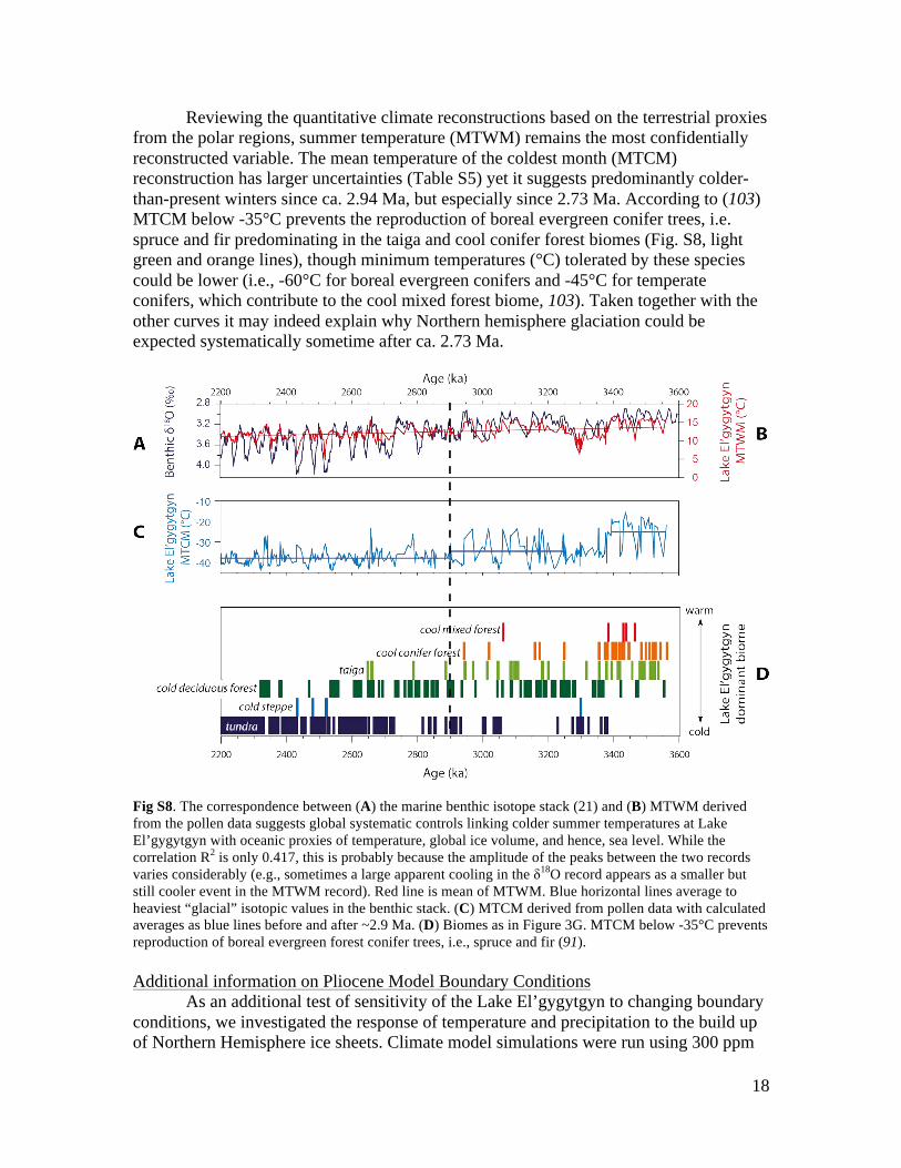
Reviewing the quantitative climate reconstructions based on the terrestrial proxies from the polar regions, summer temperature (MTWM) remains the most confidentially reconstructed variable. The mean temperature of the coldest month (MTCM) reconstruction has larger uncertainties (Table S5) yet it suggests predominantly colder-than-present winters since ca. 2.94 Ma, but especially since 2.73 Ma. According to (103) MTCM below -35°C prevents the reproduction of boreal evergreen conifer trees, i.e. spruce and fir predominating in the taiga and cool conifer forest biomes (Fig. S8, light green and orange lines), though minimum temperatures (°C) tolerated by these species could be lower (i.e., -60°C for boreal evergreen conifers and -45°C for temperate conifers, which contribute to the cool mixed forest biome, 103). Taken together with the other curves it may indeed explain why Northern hemisphere glaciation could be expected systematically sometime after ca. 2.73 Ma.

Fig S8. The correspondence between (A) the marine benthic isotope stack (21) and (B) MTWM derived from the pollen data suggests global systematic controls linking colder summer temperatures at Lake El’gygytgyn with oceanic proxies of temperature, global ice volume, and hence, sea level. While the correlation R2 is only 0.417, this is probably because the amplitude of the peaks between the two records varies considerably (e.g., sometimes a large apparent cooling in the δ18O record appears as a smaller but still cooler event in the MTWM record). Red line is mean of MTWM. Blue horizontal lines average to heaviest “glacial” isotopic values in the benthic stack. (C) MTCM derived from pollen data with calculated averages as blue lines before and after ~2.9 Ma. (D) Biomes as in Figure 3G. MTCM below -35°C prevents reproduction of boreal evergreen forest conifer trees, i.e., spruce and fir (91). Additional information on Pliocene Model Boundary Conditions

As an additional test of sensitivity of the Lake El’gygytgyn to changing boundary conditions, we investigated the response of temperature and precipitation to the build up of Northern Hemisphere ice sheets. Climate model simulations were run using 300 ppm

19

CO2 and a cold boreal summer orbit, like that at 116 ka (Table S2). The simulations broadly represent late Pliocene conditions, with an orbit favorable for the growth of Northern Hemispheric ice sheets. Two simulations were run using the GCM described above, with and without Northern Hemispheric ice sheets. Both were run to equilibrium, with climatic averages calculated from the last 10 years of the simulations. The first simulation used ice-free Northern Hemispheric boundary conditions (same as Fig. 4C), while the second simulation adds the Greenland, Laurentide, and Fennoscandian ice sheets, based on LGM ice volume from ICE 4G (104). In a simple sensitivity test, the two simulations are compared to isolate the effects of large Northern Hemispheric ice sheets on circum-Arctic climate and aridification. The simulated drying (difference in precipitation rate) in mm yr-1 resulting from the presence of large Northern Hemispheric ice sheets is shown in (Fig. S9A). Coldest monthly mean temperature (Fig. S9B) in the simulation with the ice sheets compares favorably to our proxy reconstructions after ~2.9 Ma (Fig. 2). Cooling in response to the presence of the large ice sheets is shown in figure S9C.

As found in comparable studies using global and regional climate models (e.g., 105), the mechanical forcing of the ice sheets has an important effect on the mid-tropospheric westerly flow and storm tracks. In our preliminary GCM simulations, we find the combination of dynamical effects, albedo-enhanced cooling, and expanded arctic sea-ice cover contributes to substantial circum-Arctic aridification, greater than 150 mm yr-1 in much of the central Arctic basin and parts of northern Beringia. While not definitive, these results suggest the time-averaged presence of large Northern Hemispheric ice sheets contributed to the marked drying in the Lake El’gygytgyn record after ~2.73 Ma. A detailed modeling analysis of the effect of Northern Hemispheric ice sheets, vegetation, and sea ice feedbacks on the regional climate of Lake El’gygytgyn will be the subject of future work.

20

Fig. S9. Climate model simulations using 300 ppm CO2 and a cold boreal summer orbit, like that at 116 ka (Table S2) to isolate the effects of large Northern Hemispheric ice sheets on circum-Arctic climate and aridification. (A) The simulated drying (difference in precipitation rate) in mm yr-1 resulting from the presence of large Northern Hemispheric ice sheets; (B) Coldest monthly mean temperature (MTCM) in the simulation with the ice sheets present; it compares favorably to our proxy reconstructions after ~2.9 Ma (Fig. 2). (C) 2-meter temperature differences show the circum-Arctic cooling in response to the presence of the large Northern Hemisphere ice sheets. Values are temperature difference (°C) in the model run with Northern Hemisphere ice sheets minus the ice free simulation.

References 1. J. Christensen et al., Fourth Assessment Report of the Intergovernmental Panel on

Climate Change (Cambridge Univ. Press, Cambridge, 2007) pp. 847–940.

2. M. Pagani, Z. Liu, J. LaRiviere, A. C. Ravelo, High Earth-system climate sensitivity determined from Pliocene carbon dioxide concentrations. Nat. Geosci. 3, 27 (2009). doi:10.1038/ngeo724

3. O. Seki et al., Alkenone and boron-based Pliocene pCO2 records. Earth Planet. Sci. Lett. 292, 201 (2010). doi:10.1016/j.epsl.2010.01.037

4. T. Naish et al., Obliquity-paced Pliocene West Antarctic ice sheet oscillations. Nature 458, 322 (2009). doi:10.1038/nature07867 Medline

5. J. Matthiessen, J. Knies, C. Vogt, R. Stein, Pliocene palaeoceanography of the Arctic Ocean and subarctic seas. Philos. Trans. R. Soc. London Ser. A 367, 21 (2009). doi:10.1098/rsta.2008.0203

6. H. J. Dowsett et al., The PRISM3-D paleoenvironmental reconstruction. Stratigraphy 7, 123 (2010).

7. International Commission on Stratigraphy, www.stratigraphy.org.

8. A. Z. Csank et al., Estimates of Arctic land surface temperatures during the early Pliocene from two novel proxies. Earth Planet. Sci. Lett. 304, 291 (2011). doi:10.1016/j.epsl.2011.02.030

9. A. P. Ballantyne et al., Significantly warmer Arctic surface temperatures during the Pliocene indicated by multiple independent proxies. Geology 38, 603 (2010). doi:10.1130/G30815.1

10. C. Schweger, D. G. Froese, J. M. White, J. A. Westgate, Pre-glacial and interglacial pollen records over the last 3 Ma from northwest Canada: Why do Holocene forests differ from those of previous interglaciations? Quat. Sci. Rev. 30, 2124 (2011). doi:10.1016/j.quascirev.2011.01.020

11. D.A. Darby, The Arctic perennial ice cover over the last 4 million years. Paleoceanography 23, PA1S07, doi:10.1029/ 2007PA001479 (2008), doi:10.1029/ 2007PA001479.

12. K. St. John, Cenozoic ice-rafting history in the Central Arctic: Terrigenous sands on the Lomonosov Ridge. Paleoceanography 23, PA1S05 (2008). doi:10.1029/2007PA001483

13. C. E. Stickley et al., Evidence for middle Eocene Arctic sea ice from diatoms and ice-rafted debris. Nature 460, 376 (2009). doi:10.1038/nature08163 Medline

14. R. Stein, K. Fahl, J. Müller, Proxy reconstruction of Cenozoic Arctic Ocean sea ice history – from IRD to IP25. Polarforschung 82, 37 (2012).

15. M. O’Regan, C. J. Williams, K. E. Frey, M. Jakobsson, A synthesis of the long-term paleoclimatic evolution of the Arctic. Oceanography (Wash. D.C.) 24, 66 (2011). doi:10.5670/oceanog.2011.57

2

16. L. Polyak et al., History of sea ice in the Arctic. Quat. Sci. Rev. 29, 1757 (2010). doi:10.1016/j.quascirev.2010.02.010

17. P. Layer, Argon-40/Argon-39 age of the El'gygytgyn impact event, Chukotka, Russia. Meteorit. Planet. Sci. 35, 591 (2000). doi:10.1111/j.1945-5100.2000.tb01439.x

18. M. Melles et al., 2.8 million years of Arctic climate change from Lake El’gygytgyn, NE Russia. Science 337, 315 (2012). doi:10.1126/science.1222135 Medline

19. A. S. Studer et al., Enhanced stratification and seasonality in the Subarctic Pacific upon Northern Hemisphere glaciation–New evidence from diatom-bound nitrogen isotopes, alkenones and archaeal tetraethers. Earth Planet. Sci. Lett. 351-352, 84 (2012). doi:10.1016/j.epsl.2012.07.029

20. A. J. Hidy, J. C. Gosse, D. G. Froese, J. D. Bond, D. H. Hood, A latest Pliocene age for the earliest and most extensive Cordilleran Ice Sheet in northwestern Canada. Quat. Sci. Rev. 61, 77 (2013). doi:10.1016/j.quascirev.2012.11.009

21. L. E. Lisecki, M. E. Raymo, A Pliocene-Pleistocene stack of 57 globally distributed benthic δ18O records. Paleoceanography 20, PA1003 (2005). 10.1029/2004PA001071

22. G. H. Miller et al., Temperature and precipitation history of the Arctic. Quat. Sci. Rev. 29, 1679 (2010). doi:10.1016/j.quascirev.2010.03.001

23. R. M. Deconto et al., Thresholds for Cenozoic bipolar glaciation. Nature 455, 652 (2008). doi:10.1038/nature07337 Medline

24. D. G. Froese, R. W. Barendregt, R. J. Enkin, J. Baker, Paleomagnetic evidence for multiple late Pliocene-early Pleistocene glaciations in the Klondike area, Yukon Territory. Can. J. Earth Sci. 37, 863 (2000). doi:10.1139/e00-014

25. M. Nolan, J. Brigham-Grette, Basic hydrology, limnology, and meteorology of modern Lake El’gygytgyn, Siberia. J. Paleolimnol. 37, 17 (2007). doi:10.1007/s10933-006-9020-y

26. O. Y. Glushkova, V. N. Smirnov, Pliocene to Holocene geomorphic evolution and paleogeography of the Lake El’gygytgyn Lake region, NE Russia. J. Paleolimnol. 37, 37 (2007). doi:10.1007/s10933-006-9021-x

27. O. Juschus, F. Preusser, M. Melles, U. Radtke, Applying SAR-IRSL methodology for dating fine-grained sediments from Lake El’gygytgyn, north-eastern Siberia. Quat. Geochronol. 2, 187 (2007). doi:10.1016/j.quageo.2006.05.006

28. M. Melles et al., The Lake El’gygytgyn Scientific Drilling Project – conquering Arctic challenges in continental drilling. Sci. Drill. 11, 29 (2011).

29. A. C. Gebhardt, F. Niessen, C. Kopsch, Central ring structure identified in one of the world’s best-preserved impact craters. Geology 34, 145 (2006). doi:10.1130/G22278.1

30. J. Laskar et al., A long term numerical solution for the insolation quantities of the Earth. Astron. Astrophys. 428, 261 (2004). doi:10.1051/0004-6361:20041335

3

31. J. V. Matthews Jr., A. Telka, Insect fossils from the Yukon. in Insects of the Yukon, H. V. Danks, J. A. Downes, Eds. (Biol. Surv. Canada (Terr. Arthropods), Ottawa, 1997) pp. 911–962.

32. N. Rybczynski et al., Mid-Pliocene warm-period deposits in the High Arctic yield insights into camel evolution. Nat. Commun. 4, 1550 (2013). doi:10.1038/ncomms2516

33. J. England, Glaciation and the evolution of the Canadian high arctic landscape. Geology 15, 419 (1987). doi:10.1130/0091-7613(1987)15<419:GATEOT>2.0.CO;2

34. K. T. Lawrence, T. D. Herbert, C. M. Brown, M. E. Raymo, A. M. Haywood, High-amplitude variations in North Atlantic sea surface temperature during the early Pliocene warm period. Paleoceanography 24, PA2218 (2009). doi:10.1029/2008PA001669

35. C. M. Brierley, A. V. Federov, Relative importance of meridional and zonal sea surface temperature gradients for the onset of the ice ages and Pliocene-Pleistocene climate Evolution. Paleoceanography 25, PA2214 (2010). doi:10.1029/2009PA001809

36. T. D. Herbert, L. C. Peterson, K. T. Lawrence, Z. Liu, Tropical ocean temperatures over the past 3.5 million years. Science 328, 1530 (2010). doi:10.1126/science.1185435 Medline

37. R. McKay et al., Antarctic and Southern Ocean influences on Late Pliocene global cooling. Proc. Natl. Acad. Sci. U.S.A. 109, 6423 (2012). doi:10.1073/pnas.1112248109 Medline

38. S. Levis, J. A. Foley, D. Pollard, Potential high-latitude vegetation feedbacks on CO2-induced climate change. Geophys. Res. Lett. 26, 747 (1999). doi:10.1029/1999GL900107

39. S. J. Koenig, R. M. DeConto, D. Pollard, Late Pliocene to Pleistocene sensitivity of the Greenland Ice Sheet in response to external forcing and internal feedbacks. Clim. Dyn. 37, 1247 (2011). doi:10.1007/s00382-011-1050-0

40. A. A. Andreev et al., Late Pliocene/Early Pleistocene environments of the north-eastern Siberia inferred from Lake El’gygytgyn pollen record. 12th Intern Paleolim Symposium-Glasgow, 21-24 August 2012, p. 197.

41. G. H. Haug et al., North Pacific seasonality and the glaciation of North America 2.7 million years ago. Nature 433, 821 (2005). doi:10.1038/nature03332 Medline

42. S. A. Elias, J. V. Matthews, Jr., Arctic North American seasonal temperatures from the latest Miocene to the Early Pleistocene, based on mutual climatic range analysis of fossil beetle assemblages. Can. J. Earth Sci. 39, 911 (2002). doi:10.1139/e01-096

43. A. M. Haywood et al., Large-scale features of Pliocene climate: Results form the Pliocene Model Intercomparison Project. Clim. Past 8, 2969 (2012). doi:10.5194/cpd-8-2969-2012

4

44. D. S. Kaufman et al., Holocene thermal maximum in the western Arctic (0-180°W). Quat. Sci. Rev. 23, 529 (2004). doi:10.1016/j.quascirev.2003.09.007

45. E. Jansen, T. Fronval, F. Rack, J. E. T. Channell, Pliocene-Pleistocene ice rafting history and cyclicity in the Nordic Seas during the last 3.5 Myr. Paleoceanography 15, 709 (2000). doi:10.1029/1999PA000435

46. G. S. Dwyer, M. A. Chandler, Mid-Pliocene sea level and continental ice volume based on coupled benthic Mg/Ca palaeotemperatures and oxygen isotopes. Philos. Trans. A Math. Phys. Eng. Sci. 367, 157 (2009). doi:10.1098/rsta.2008.0222 Medline

47. S. De Schepper, M. J. Head, J. Groeneveld, North Atlantic Current variability through marine isotope stage M2 (circa 3.3 Ma) during the mid-Pliocene. Paleoceanography 24, PA4206 (2009). doi:10.1029/2008PA001725

48. D. Pollard, R. M. DeConto, Modelling West Antarctic ice sheet growth and collapse through the past five million years. Nature 458, 329 (2009). doi:10.1038/nature07809 Medline

49. K. T. Lawrence, S. Sosdian, H. E. White, Y. Rosenthal, North Atlantic climate evolution through the Plio-Pleistocene climate transitions. Earth Planet. Sci. Lett. 300, 329 (2010). doi:10.1016/j.epsl.2010.10.013

50. J. Knies et al., The Plio-Pleistocene glaciation of the Barents Sea–Svalbard region: a new model based on revised chronostratigraphy. Quat. Sci. Rev. 28, 812 (2009). doi:10.1016/j.quascirev.2008.12.002

51. M. E. Raymo, J. X. Mitrovica, M. J. O’Leary, R. M. DeConto, P. J. Hearty, Departures from eustasy in Pliocene sea-level records. Nat. Geosci. 4, 328 (2011). doi:10.1038/ngeo1118

52. A. Duk-Rodkin, R. W. Barendregt, J. M. White, An extensive late Cenozoic terrestrial record of multiple glaciations preserved in the Tintina Trench of west-central Yukon: stratigraphy, paleomagnetism, paleosols, and pollen. Can. J. Earth Sci. 47, 1003 (2010). doi:10.1139/E10-060

53. G. Balco, C. W. Rovey, Absolute chronology for major Pleistocene advances of the Laurentide Ice Sheet. Geology 38, 795 (2010). doi:10.1130/G30946.1

54. P. U. Clark, D. Pollard, Origin of the middle Pleistocene transition by ice sheet erosion of regolith. Paleooceanography 13, 1 (1998). doi:10.1029/97PA02660

55. K. G. Miller et al., High tide of the warm Pliocene: Implications of global sea level for Antarctic deglaciation. Geology 40, 407 (2012). doi:10.1130/G32869.1

56. T. D. Hamilton, K. Reed, R. Thorson, Glaciation in Alaska: the Geologic Record (Alaska Geol. Soc., Anchorage, AK, 1986).

57. K. Takahashi et al., IODP Expedition 323-Pliocene and Pleistocene paleoceanographic changes in the Bering Sea. Sci. Drill. 11, 4 (2011).

58. M. Nolan, Analysis of local AWS and NCEP/NCAR reanalysis data at Lake El'gygytgyn, and its implications for maintaining multi-year lake-ice covers. Clim. Past Disc 8, 1443 (2012). doi:10.5194/cpd-8-1443-2012

5

59. C. M. Brierley et al., Greatly expanded tropical warm pool and weakened Hadley circulation in the early Pliocene. Science 323, 1714 (2009). doi:10.1126/science.1167625 Medline

60. A. Prokopenko et al., The link between tectonic and paleoclimatic events at 2.8-2.5 Ma BP in the Lake Baikal region. Quat. Int. 80-81, 37 (2001). doi:10.1016/S1040-6182(01)00017-9

61. J. Brigham-Grette, L. D. Carter, Pliocene marine transgressions of northern Alaska: Circumarctic Correlations and Paleoclimate. Arctic 43, 74 (1992).

62. G. Bartoli, B. Hönisch, R. E. Zeebe, Atmospheric CO2 decline during the Pliocene intensification of Northern Hemisphere Glaciations. Paleoceanography 26, PA4213 (2011). doi:10.1029/2010PA002055

63. M. New, D. Lister, M. Hulme, I. Makin, A high-resolution data set of surface climate over global land areas. Clim. Res. 21, 1 (2002). doi:10.3354/cr021001

64. J. Brigham-Grette, M. Melles, P. Minyuk, and Scientific Party, Overview and Significance of a 250 ka Paleoclimate Record from El’gygytgyn Crater Lake, NE Russia. J. Paleolimnol. 37, 1 (2007). doi:10.1007/s10933-006-9017-6

65. O. Juschus, M. Melles, A. C. Gebhardt, F. Niessen, Late Quaternary mass movement events in Lake El′gygytgyn, North-eastern Siberia. Sedimentology 56, 2155 (2009). doi:10.1111/j.1365-3091.2009.01074.x

66. M. Melles et al., Sedimentary geochemistry of core PG1351 from Lake El’gygytgyn—a sensitive record of climate variability in the East Siberian Arctic during the past three glacial–interglacial cycles. J. Paleolimnol. 37, 89 (2007). doi:10.1007/s10933-006-9025-6

67. M.-S. C. L. Geotek, (2000; http://www.geotek.co.uk/).

68. L. Löwemark et al., Normalizing XRF-scanner data: A cautionary note on the interpretation of highresolution records from organic-rich lakes. J. Asian Earth Sci. 40, 1250 (2011). doi:10.1016/j.jseaes.2010.06.002

69. H. Guyard et al., High-altitude varve records of abrupt environmental changes and mining activity over the last 4000 years in the western French Alps (Lake Bramant, Grandes Rousses Massif). Quat. Sci. Rev. 26, 2644 (2007). doi:10.1016/j.quascirev.2007.07.007

70. P. Rosén et al., Universally applicable model for the quantitative determination of lake sediment composition using fourier transform infrared spectroscopy. Environ. Sci. Technol. 45, 8858 (2011). doi:10.1021/es200203z Medline

71. A. I. Best, D. E. Gunn, Calibration of marine sediment core loggers for quantitative acoustic impedance studies. Mar. Geol. 160, 137 (1999). doi:10.1016/S0025-3227(99)00017-1

72. S. Gerland, G. Kuhn, G. Bohrmann, Physical properties of a porcellanite layer (Southwest Indian Ridge) constrained by geophysical logging. Mar. Geol. 140, 415 (1997). doi:10.1016/S0025-3227(97)00046-7

73. T. J. Bralower, H. R. Thierstein, in Marine Petroleum Source Rocks, J. Brooks, A. J. Fleet, Eds. (Geol. Soc. Spec. Publ. 26, London, 1987), pp. 345-369.

6

74. PALE Steering Committee, Research Protocols for PALE: Paleoclimate of Arctic Lakes and Estuaries (PAGES Workshop Rep. Ser., 1994).

75. B. van Geel, in Tracking Environmental Change Using Lake Sediments Volume 3: Terrestrial, Algal and Silicaceous Indicators, J.P. Smol, H.J.B. Birks and W.M. Last, Eds. (Kluwer, Dordrecht, 2001), pp. 99-119.

76. S. L. Thompson, D. Pollard, Greenland and Antarctic mass balances for present and doubled atmospheric CO2 from the GENESIS Version-2 Global Climate Model. J. Clim. 10, 871 (1997). doi:10.1175/1520-0442(1997)010<0871:GAAMBF>2.0.CO;2

77. J. O. Kaplan et al., Climate change and Arctic ecosystems: 2. Modeling, paleodata-model comparisons, and future projections. J. Geophys. Res. 108, (D19), 8171 (2003). doi:10.1029/2002JD002559

78. J. T. Kiehl et al., The National Center for Atmospheric Research Community Climate Model: CCM3. J. Clim. 11, 1131 (1998). doi:10.1175/1520-0442(1998)011<1131:TNCFAR>2.0.CO;2

79. A. Berger, M. F. Loutre, Insolation values for the climate of the last 10 million of years. Quat. Sci. Rev. 10, 297 (1991). doi:10.1016/0277-3791(91)90033-Q

80. D. S. Kaufman, J. Brigham-Grette, Aminostratigraphic correlations and paleotemperature implications, Pliocene-Pleistocene high sea level deposits, northwestern Alaska. Quat. Sci. Rev. 12, 21 (1993). doi:10.1016/0277-3791(93)90046-O

81. J. G. Fyles et al., Ballast Brook and Beaufort Formations (Late Tertiary) on northern Banks Island, Arctic Canada. Quat. Int. 22-23, 141 (1994). doi:10.1016/1040-6182(94)90010-8

82. J. G. Fyles, L. Marincovich Jr., J. V. Mathews Jr., R. Barendregt, in Current Research, Part B. Paper 91- 1B (Geol. Surv. of Can., Ottawa, 1991), pp. 461-468.

83. J. G. Fyles et al., Geology of Hvitland Beds (late Pliocene), White Point Lowland, Ellesmere Island, Northwest Territories (Geol. Surv. Can. Bull. 1998), vol. 512, 35 pp.

84. J. Böcher, Paleoentomology of the Kab Købnhavn Formation, a Plio-Pleistocene sequence in Peary Land, North. Medd. Gronl. Geosci. 33, 1 (1995).

85. O. Bennike, The Kap København Formation: Stratigraphy and paleobotany of a Pliocene-Pleistocene sequence in Peary Land, North Greenland. Medd. Gronl. Geosci. 23, 1 (1990).

86. S. Funder et al., Late Pliocene Greenland: the Kap København formation in North Greenland. Bull. Geol. Soc. Den. 48, 177 (2001).

87. R. W. Feyling-Hanssen, The Lodin Elv Formation: a Pliocene-Pleistocene occurrence in Greenland. Bull. Geol. Soc. Den. 31, 81 (1983).

88. C. I. Prentice, J. Guiot, B. Huntley, D. Jolly, R. Cheddadi, Reconstructing biomes from palaeoecological data: A general method and its application to European pollen data at 0 and 6 ka. Clim. Dyn. 12, 185 (1996). doi:10.1007/BF00211617

7

89. P. E. Tarasov et al., Present day and mid-Holocene biomes reconstructed from pollen and plant macrofossil data from the former Soviet Union and Mongolia. J. Biogeogr. 25, 1029 (1998). doi:10.1046/j.1365-2699.1998.00236.x

90. M. E. Edwards et al., Pollen-based biomes for Beringia 18,000, 6000 and 0 14C yr BP. J. Biogeogr. 27, 521 (2000). doi:10.1046/j.1365-2699.2000.00426.x

91. P. E. Tarasov et al., Last Glacial Maximum biomes reconstructed from pollen and plant macrofossil data from Northern Eurasia. J. Biogeogr. 27, 609 (2000). doi:10.1046/j.1365-2699.2000.00429.x

92. P. E. Tarasov et al., Quantitative reconstruction of the Last Interglacial vegetation and climate based on the pollen record from Lake Baikal, Russia. Clim. Dyn. 25, 625 (2005). doi:10.1007/s00382-005-0045-0

93. S. Müller et al., Late Quaternary vegetation and environments in the Verkhoyansk Mountains region (NE Asia) reconstructed from a 50-kyr fossil pollen record from Lake Billyakh. Quat. Sci. Rev. 29, 2071 (2010). doi:10.1016/j.quascirev.2010.04.024

94. P. M. Anderson, A. V. Lozhkin, L. B. Brubaker, Implications of a 24,000-Yr palynological record for a Younger Dryas cooling and for Boreal forest development in northeastern Siberia. Quat. Res. 57, 325 (2002). doi:10.1006/qres.2002.2321

95. P. E. Tarasov et al., Progress in the reconstruction of Quaternary climate dynamics in the Northwest Pacific: a new modern analogue reference dataset and its application to the 430-kyr pollen record from Lake Biwa. Earth Sci. Rev. 108, 64 (2011). doi:10.1016/j.earscirev.2011.06.002

96. L. Mokhova, P. E. Tarasov, V. Bazarova, M. Klimin, Quantitative biome reconstruction using modern and late Quaternary pollen data from the southern part of the Russian Far East. Quat. Sci. Rev. 28, 2913 (2009). doi:10.1016/j.quascirev.2009.07.018

97. J. Guiot, C. Goeury, PPPBASE, a software for statistical analysis of palaeoecological and palaeoclimatological data. Dendrochronologia 14, 295 (1996).

98. J. T. Overpeck, T. Webb III, I. C. Prentice, Quantitative interpretation of fossil pollen spectra: Dissimilarity coefficients and the method of modern analogs. Quat. Res. 23, 87 (1985). doi:10.1016/0033-5894(85)90074-2

99. T. Nakagawa, P. E. Tarasov, K. Nishida, K. Gotanda, Y. Yasuda, Quantitative pollen-based climate reconstruction in central Japan: Application to surface and late Quaternary spectra. Quat. Sci. Rev. 21, 2099 (2002). doi:10.1016/S0277-3791(02)00014-8

100. Polation (version 1.1) and Polygon (version 2.3.3) computer programs, http://dendro.narutou.ac.jp/~nakagawa/ (2012).

101. C2 computer program, version 1.7.2, www.staff.ncl.ac.uk/staff/stephen.juggins/software/C2Home.htm (2012).

8

102. J. Guiot, Methodology of the last climatic cycle reconstruction in France from pollen data. Palaeogeogr. Palaeoclimatol. Palaeoecol. 80, 49 (1990). doi:10.1016/0031-0182(90)90033-4

103. I. C. Prentice et al., A global biome model based on plant physiology and dominance, soil properties, and climate. J. Biogeogr. 19, 117 (1992). doi:10.2307/2845499

104. W. R. Peltier, Ice age topography. Science 265, 195 (1994). doi:10.1126/science.265.5169.195

105. D. H. Bromwich et al., Polar MM5 Simulations of the Winter Climate of the Laurentide Ice Sheet at the LGM. J. Clim. 17, 3415 (2004). doi:10.1175/1520-0442(2004)017<3415:PMSOTW>2.0.CO;2