ii

“CATS” — 2017/3/19 — 20:35 — page 1 — #10 ii

ii

ii

CATS for protein design backbone flexibility 1

Supplementary Material

The following is optional Supplementary Material (SM) thatprovides additional information to substantiate the claims of thepaper. SM 1 provides details on the peptide-plane geometry assumptionsand how they are encoded as equality constraints on the backbone atomcoordinates. SM 2 provides a summary of the CATS algorithm. SM 3provides a proof of Theorem 1. SM 4 discusses the computationalcomplexity of CATS. SM 5 provides details of the Taylor seriescomputation used in CATS. SM 6 provides details of the protein designtest cases described in Section 3.1. References cited below are given in theReferences section of the main text.

1 Details of peptide plane geometry assumptionsAs mentioned in Section 2.2, we assume (1) that peptide planes are rigidbodies, and (2) that the N-C

↵

-C0 bond angle in each residue is fixed.Crystal structures show that these assumptions are nearly correct (Lovellet al., 2003). CATS could be extended to model slight perturbations tothese assumptions. But we will not do so here, since doing so wouldproduce only marginal changes in other atomic interactions. Moreover, theextent of these changes depends on the balance between two completelydifferent types of energies—bond length and angle distortion penaltiesversus small changes in other interaction energies like van der Waalsand electrostatic energies. It is not clear that current energy functionshave sufficient quantitative accuracy to make estimation of this balanceworthwhile. Our approach here is analogous to the usual approach takenin continuously flexible protein design for sidechains (Desmet et al., 1992;Leach and Lemon, 1998; Desmet et al., 2002; Georgiev et al., 2008b;Gainza et al., 2012), which moves only the sidechain dihedrals whilefixing the bond lengths and angles.

Given that the peptide plane is rigid, the conformation of the entireplane is determined by the coordinates of any three of its atoms. Thus, ifwe determine the coordinates of the two alpha carbons and the nitrogenatom in a peptide plane, the coordinates of any other backbone atoms willbe fixed in a basis defined by these three atoms. For each other backboneatom n (the carbonyl carbon, oxygen, or amide hydrogen), we calculatethe coordinates of n in this basis from the starting structure, and thenuse those coordinates whenever we move the alpha carbons and nitrogensusing CATS. We use coordinates from the starting structure instead ofidealized coordinates because we wish to include the original backboneconformation in the CATS search space.

Even the alpha-carbon and nitrogen atoms cannot move entirely freely:they have only two rather than six degrees of freedom per residue. We thusadd four additional constraints on atom-atom distances (Fig. S1). Thefirst three constraints reflect the need for the peptide plane to move onlyas a rigid body. To enforce this, we fix the side lengths of the triangleformed by the nitrogen and two alpha carbons in each peptide plane.Because triangles whose side lengths are equal are congruent, the peptideplane is restricted to rigid-body motions if and only if these three distanceconstraints are enforced. Finally, to constrain the N-C

↵

-C0 bond angle, wefix the dot product of the N-C

↵

and C↵

-C0 bond vectors. Given peptideplane geometry, the lengths of these two bonds are fixed, so our dot productconstraint fixes the angle. The imposed values of these distances and dotproduct are taken from the original crystal structure. Again, this is doneto ensure the original backbone conformation is part of the search space.Thus, these constraints, together with the linear formula for the otherbackbone coordinates, ensures the N-C

↵

-C0 bond angle will not changerelative to the starting structure, while the peptide planes will only moveas rigid bodies relative to that structure.

There are four constrained quantities per residue: the squares of theside lengths of the triangle of atoms defining each peptide plane, and thedot product of the N-C

↵

and C↵

-C0 bond vectors (see Fig. S1). Thus c

(see Eq. (3)) has four components per peptide plane, which are as follows:

||a(C↵

, 1)� a(C↵

, 2)||2 (5)

||a(C↵

, 1)� a(N, 2)||2 (6)

||a(N, 2)� a(C↵

, 2)||2 (7)

(a(C↵

, 1)� a(N, 1)) · (a(C↵

, 1)� a(C0, 1)) (8)

where a(n, i) denotes the coordinates of atom n of residue i; withoutloss of generality we set i = 1 for the first residue of the peptide plane.For purposes of the last constraint (Eq. 8), the coordinates of the carbonylcarbon C0 are expressed as a linear combination of the nitrogen and alpha-carbon coordinates. Thus in the case that the peptide plane is not exactlyplanar, we are actually constraining the projection of C0 into the plane ofthe nitrogens and alpha carbons, which has essentially the same physicaleffect but is much simpler mathematically.

2 Summary of algorithmAs discussed in Section 2.1, protein design algorithms likeiMinDEE (Gainza et al., 2012) and EPIC (Hallen et al., 2015) convertthe continuous degrees of freedom over which they search to all-atomcoordinates in order to evaluate energy as a function of the degrees offreedom, and thus design for energetically optimal sequences. We presenthere a summary of this conversion. The conversion function is called a(x)

in the text and is described primarily in Section 2.3.Before beginning design, we perform initialization calculations, which

define the degrees of freedom. Let ab0

be the initial backbone coordinatesof the molecule (e.g., from the crystal structure), and for a vector z ofcoordinates let z(p, n) denote the coordinates in z of the atom named n

in peptide plane p (each peptide plane has two alpha carbons, which wecall C

↵1 and C↵2). We initialize as follows:

ii

“CATS” — 2017/3/19 — 20:35 — page 2 — #11 ii

ii

ii

2 Hallen and Donald

Fig. S1. Geometry assumptions in a section of protein backbone. Each peptide plane moves as a rigid body. This condition is enforced by holding three distances constant (straight purplearrows) and fixing the coordinates of C0 and backbone oxygens and hydrogens in the reference frame of the N and C↵ coordinates. We also hold the N-C↵-C0 angle constant (curvedarrow); both the distance and angle constraints are expressed as quadratic equalities in the N and C↵ coordinates (see SM 1 for details). These constrained quantities are invariant whenthe backbone dihedrals are rotated (thus, as can be see in the left vs. right panels, they keep the same values). For example, the triangles formed by the straight purple arrows in the twoconformations are congruent.

y

0

N-and-C↵

-Coordinates(ab0

)

// Now we express ab0

as a function of y0

, represented as coefficientsv

// Loop over all peptide planes containing flexible backbone atomsfor all p in FlexiblePeptidePlanes doz

1

a

b0

(p,N)� a

b0

(p,C↵1)

z

2

a

b0

(p,C↵2)� a

b0

(p,C↵1)

Q

p

[z1

, z

2

, z

1

⇥ z

2

] // make a basis for this peptide plane; ⇥denotes cross productfor all n in C0, O, H dov(p, n) Q

�1p

a

b0

(p, n) // These coefficients will stay constant// as N and C

↵

coords, and thus Qp

, changeend for

end for

// Compute the linear coefficients to define our backbone degrees offreedomM

y

nullspace(rc(y0

)) //My

has orthonormal rows,// which are orthogonal to the rows ofrc(y

0

)

// Compute the constraintsc

0

c(y0

) // see c definition in Eqs. (5)-(8)

// We now have everything we need to define f

// we now compute derivatives to find the series expansion of f�1

p ComputeTaylorSeriesCoefficients(ab0

, c

0

,v,M

y

) // SeeEq. (11)

Then a(x) is computed as follows, where x is the vector of valuesof the continuous conformational degrees of freedom. The function a(x)

uses the coefficients v and p as parameters:

(xb

,�) x// unpack x into backbone degrees of freedom andsidechain dihedralsy p(x

b

) // compute nitrogen and alpha-carbon coordinates// Now fill in the rest of y (other atoms’ coordinates)for all p in FlexiblePeptidePlanes do

// compute other backbone coordinatesz

1

y(p,N) � y(p,C↵1) // y(p, n) denotes coordinates in y for

atom n in p

z

2

y(p,C↵2)� y(p,C

↵1)

Q

p

[z1

, z

2

, z

1

⇥ z

2

]) // make a basis for this peptide planefor all n in C0, O, H doy(p, n) Q

p

v(p, n) // compute coordinates of atom n in plane pend for

end for

// Place idealized sidechains (see Hallen et al., 2013; Lovell et al., 2003)in coordinates yy PlaceIdealizedSidechains(y)y RotateSidechains(y,�) // Apply the sidechain dihedral degrees offreedomReturn y

3 Proof of Theorem 1Theorem 1. Let D

b

denote the directional derivative in directionb. If z(y) = M

z

y + v

z

is an affine function and c satisfies|r(c(y

0

)T ) M

T

z

| 6= 0, then there exists an affine bijection betweenZ = {x

b

2 R2k�6 |xb

6= 0} and B = {b 2 R6k |b 6=0, D

b

c(y0

) = 0}.

Proof. Letting f = {c,xb

} and J = rf(y0

), consider the mappingm where m(b) consists of the last 2k� 6 components of J ·b. From theassumptions in the theorem, we have |J | 6= 0, i.e., the Jacobian of f(y

0

)

is nonsingular. Also J

�1 is well defined, which allows us to construct theinverse mapping m

�1: for any x

b

2 Z, m�1(xb

) = J

�1 · {0,xb

}.Thus both m and its inverse are affine.

For any x

b

2 Z,

D

m

�1(xb)c(y0

) = rc(y0

) ·m�1(xb

), (9)

which consists of the first 4k + 6 components of

J ·m�1(xb

) = J · J�1 · {0,xb

} = {0,xb

}. (10)

ii

“CATS” — 2017/3/19 — 20:35 — page 3 — #12 ii

ii

ii

CATS for protein design backbone flexibility 3

Thus the first 4k+6 components of Eq. (10) are 0, making Eq. (9) evaluateto 0. Also, J�1 is nonsingular, so m

�1(xb

) cannot be 0. Thus for anyx

b

2 Z, m�1(xb

) 2 B.For anyb 2 B, m(b) = 0would imply J ·b = 0, which contradicts

J being nonsingular. Thus for any b 2 B, m(b) 6= 0 and so m(b) 2 Z.Therefore, m is an affine bijection between B and Z.

4 Computational complexity of CATSIn the worst case, the asymptotic complexity of CATS is the same as forrigid-backbone design with the same sequence space. CATS and rigid-backbone design (as performed with iMinDEE (Gainza et al., 2012), forexample) create an RC for each sidechain rotamer; the only differenceis that the CATS RC includes backbone degrees of freedom while theiMinDEE RC does not. Suppose there are n mutable positions and q

rotamers per mutable position. The conformational space of the entiresystem then consists of qn voxels, representing all possible combinationsof RCs at different residues. In the worst case (Pierce and Winfree, 2002;Chazelle et al., 2004), the minimized energy (Eq. 2) must be computedseparately for each voxel, so both iMinDEE and CATS have worst-casecomplexity O(qn).

In practice, pruning of RCs using dead-end elimination (Desmetet al., 1992; Georgiev et al., 2008b; Gainza et al., 2012) and boundingof the minimum energies of portions of conformational space as partof A* search (Leach and Lemon, 1998; Georgiev et al., 2008b; Gainzaet al., 2012; Hallen et al., 2015) ensure that the vast majority of voxelswill not require their own energy minimization—neither in CATS nor iniMinDEE. CATS has been implemented to use the EPIC algorithm aspart of its conformational search, which tightens energy bounds comparedto iMinDEE alone (Hallen et al., 2015). Nevertheless, energy bounds inA*-based protein design (Leach and Lemon, 1998; Gainza et al., 2012;Hallen et al., 2015) tend to become looser as more flexibility is added,causing a greater number of energy minimizations to be performed. Thisfact, together with the fact that each minimization takes longer when thereare more degrees of freedom, causes CATS designs to almost always takelonger than comparable rigid-backbone designs.

5 Constructing and validating the Taylor seriesFor each voxel, we construct a Taylor series to evaluate the inversemapping from Section 2.3, which we write as f�1({c,x

b

}) without lossof generality. We need only evaluate this mapping for c = c

0

, that is, withthe constrained quantities kept at the values measured using the startingstructure (see Section 2.2). Hence, the Taylor series will be centered atx

b

=0 and c at c0

, and all terms in the series that contain a component ofc will be 0:

y = f

�1({c0

,x

b

}) = y

0

+@f

�1

@x

b

· xb

+1

2x

b

· @2f

�1

@x

b

2· x

b

+ ...

(11)

where derivatives are evaluated at the central conformation (xb

= 0). Toevaluate these derivatives, we observe that the derivatives of f = {c, z}with respect to the atomic coordinates y can be evaluated analytically(since z and c are linear and quadratic functions of y respectively), andthe derivatives for the inverse mapping can be obtained from these. Forexample, the derivatives @f

�1

@xbare components of (rf)�1.

The error in the truncated Taylor series converges to 0 as we approachthe central conformation, as is always the case for Taylor series. But wemust determine how large we can make the voxel without significant error.To do this, we start with a voxel whose range is [-1 Å,1 Å] for eachdegree of freedom, sample x

b

randomly in the voxel (50 samples per

Fig. S2. Distribution of voxel size (range of allowed values for each degree of freedom,in Å), selected as described in SM 5.

voxel), and evaluate the average error in the constrained dot productsand squared distances c(a

n

(xb

)) calculated at these samples using thetruncated series (Eq. 11). If the error is too large, we reduce the allowedrange by a factor of 1.3 and repeat validation. This sampling process isanalogous to validation in machine learning, although the model we arevalidating is the analytically-calculated Taylor series rather than a modelinferred from training data.

We use a fairly stringent criterion for the constraints (RMS error 0.01 Å), but still typically obtain a voxel ⇠1 Å across (see SM 6 andFig. S2). Since we wish to choose voxels small enough to admit localminimization, we believe that searches of larger portions of backboneconformational space should split that space into multiple backbonevoxels (Roberts and Donald, 2015). Thus, in this study we consider itsufficient to truncate the Taylor series at second order, though our codesupports up to a fourth-order series. Based on visualization of the voxels,we believe that local minimization is a relatively good approximation forglobal minimization for our voxels (see Fig. S3).

ii

“CATS” — 2017/3/19 — 20:35 — page 4 — #13 ii

ii

ii

4 Hallen and Donald

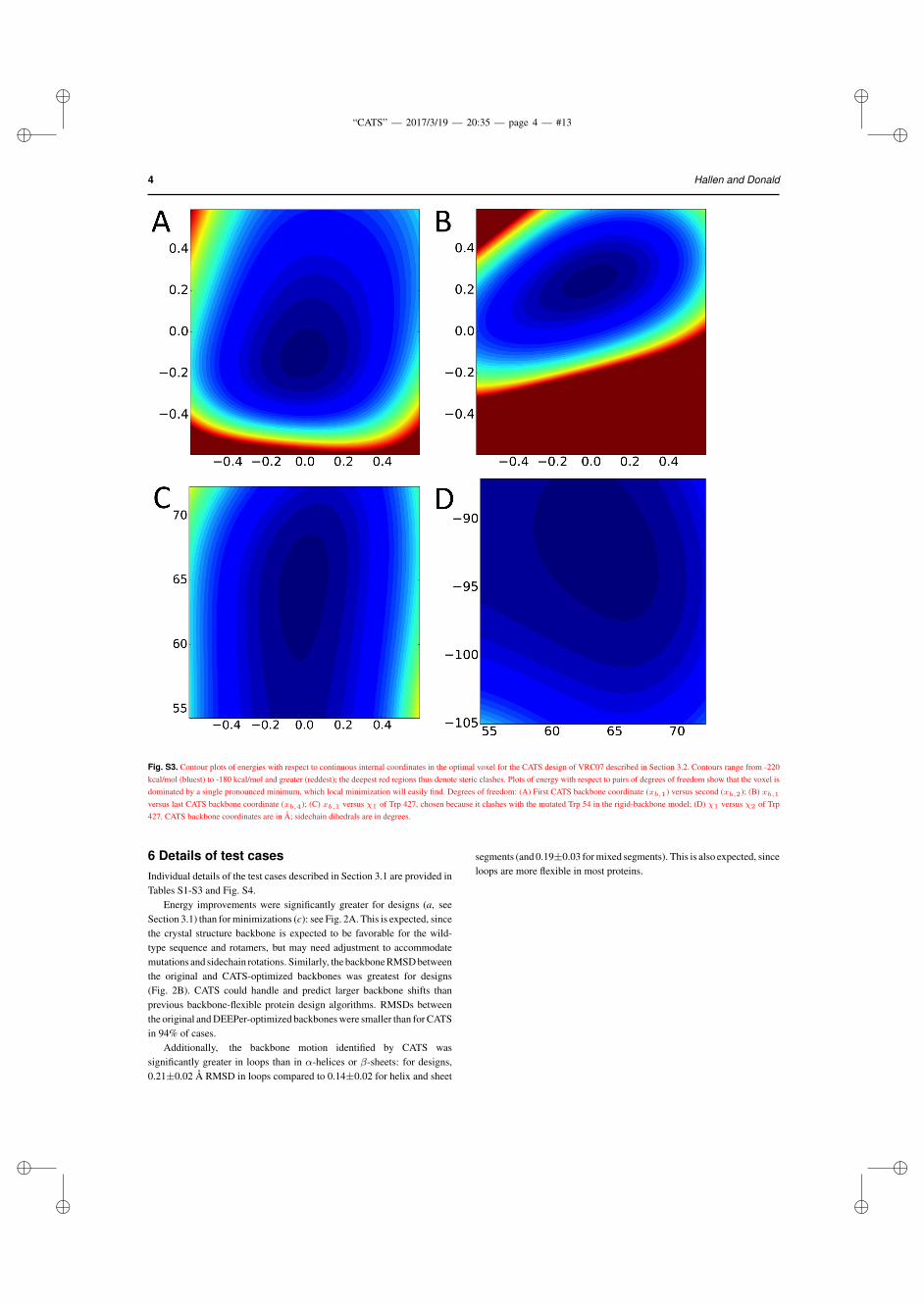
Fig. S3. Contour plots of energies with respect to continuous internal coordinates in the optimal voxel for the CATS design of VRC07 described in Section 3.2. Contours range from -220kcal/mol (bluest) to -180 kcal/mol and greater (reddest); the deepest red regions thus denote steric clashes. Plots of energy with respect to pairs of degrees of freedom show that the voxel isdominated by a single pronounced minimum, which local minimization will easily find. Degrees of freedom: (A) First CATS backbone coordinate (xb,1) versus second (xb,2); (B) xb,1

versus last CATS backbone coordinate (xb,4); (C) xb,1 versus �1 of Trp 427, chosen because it clashes with the mutated Trp 54 in the rigid-backbone model; (D) �1 versus �2 of Trp427. CATS backbone coordinates are in Å; sidechain dihedrals are in degrees.

6 Details of test casesIndividual details of the test cases described in Section 3.1 are provided inTables S1-S3 and Fig. S4.

Energy improvements were significantly greater for designs (a, seeSection 3.1) than for minimizations (c): see Fig. 2A. This is expected, sincethe crystal structure backbone is expected to be favorable for the wild-type sequence and rotamers, but may need adjustment to accommodatemutations and sidechain rotations. Similarly, the backbone RMSD betweenthe original and CATS-optimized backbones was greatest for designs(Fig. 2B). CATS could handle and predict larger backbone shifts thanprevious backbone-flexible protein design algorithms. RMSDs betweenthe original and DEEPer-optimized backbones were smaller than for CATSin 94% of cases.

Additionally, the backbone motion identified by CATS wassignificantly greater in loops than in ↵-helices or �-sheets: for designs,0.21±0.02 Å RMSD in loops compared to 0.14±0.02 for helix and sheet

segments (and 0.19±0.03 for mixed segments). This is also expected, sinceloops are more flexible in most proteins.

ii

“CATS” — 2017/3/19 — 20:35 — page 5 — #14 ii

ii

ii

CATS for protein design backbone flexibility 5

Fig. S4. Energy improvement for CATS compared to rigid-backbone design (kcal/mol),versus RMSD between CATS and original backbones (Å), in design (blue), sidechainplacement (red), and single-voxel minimization (green) test cases. As in Section 3.1, designcases search a large sequence space, sidechain placements search the conformation spaceof the the wild-type sequence, and single-voxel minimizations search the voxel around thewild-type backbone and sidechain conformations.

ii

“CATS” — 2017/3/19 — 20:35 — page 6 — #15 ii

ii

ii

6 Hallen and Donald

Table S1. Design test cases. n denotes the number of residues in the flexiblebackbone segment, which can be in loop (Y), non-loop (N), or mixed (M)secondary structure. Ec and Ed denote the improvements in minimum energyfor CATS and DEEPer runs respectively compared to rigid-backbone design.DNF denotes that a run did not finish in the allotted time (six weeks; we donot count these toward the 80 test cases), and F denotes failure of continuousminimization as described in Hallen et al., 2016. RMSDc and RMSDd denotethe backbone RMSD (over the flexible backbone segment) between the optimalconformations calculated by CATS and DEEPer respectively and the startingbackbone.w denotes the width of the voxel (the range over which each backbonedegree of freedom was allowed to vary). SD denotes sequence differencesbetween corresponding rigid-backbone (left) and CATS (right) designs.

Protein redesigned n PDB id Loop? E

c

E

d

RMSDc

RMSDd

w SDAtx1 metallochaperone 7 1CC8 Y -1.71 -1.35 0.27 0.07 1.18PA-I lectin 6 1L7L Y -3.97 -2.93 0.19 0.07 0.91 A!T, E!Dalpha-D-glucuronidase 5 1L8N Y -4.52 -1.88 0.14 0.05 0.91Dachshund 8 1L8R Y -17.08 F 0.31 F 0.91Cytochrome c 8 1M1Q Y -1.47 -0.53 0.17 0.06 0.91 S!THistidine triad protein 8 2CS7 Y -2.64 -1.57 0.22 0.05 1.18Ponsin 7 2O9S Y -3.99 -2.68 0.20 0.05 0.70Transcriptional regulator AhrC 6 2P5K Y -1.13 -0.45 0.27 0.04 0.70Scytovirin 5 2QSK Y -0.30 -0.32 0.10 0.06 0.54Hemolysin 9 2R2Z Y DNF -1.70 DNF 0.05 0.91Bucandin 7 1F94 M -1.17 -0.13 0.26 0.02 1.18Ferredoxin 9 1IQZ M F -2.78 F 0.06 1.18gamma-glutamyl hydrolase 5 1L9X M -0.69 -0.59 0.09 0.05 0.70Sulfite oxidase 7 1MJ4 M DNF -5.22 DNF 0.06 0.54Dihydrofolate reductase 6 2RH2 M -3.27 -2.48 0.24 0.04 0.91 V!L, Y!WPutative monooxygenase 7 2RIL M -2.63 -1.17 0.14 0.06 0.41alpha-crystallin 6 2WJ5 M -1.68 -0.84 0.15 0.04 0.91Cytochrome c555 7 2ZXY M -0.35 -0.34 0.20 0.03 0.91 D!EHigh-potential iron-sulfur protein 6 3A38 M -6.83 -5.66 0.26 0.07 0.91 M!WScorpion toxin 7 1AHO N -1.43 -0.45 0.12 0.04 1.18Cytochrome c553 6 1C75 N -0.91 0.03 0.16 0.10 0.70Nonspecific lipid-transfer protein 6 1FK5 N -4.31 -1.80 0.20 0.11 0.91Transcription factor IIF 7 1I27 N DNF -0.62 DNF 0.12 1.18Fructose-6-phosphate aldolase 6 1L6W N -0.84 -0.83 0.12 0.09 1.18Cephalosporin C deacetylase 8 1L7A N -5.47 -3.45 0.11 0.14 0.91Phosphoserine phosphatase 7 1L7M N DNF -3.49 DNF 0.06 0.70Granulysin 7 1L9L N -13.65 -9.75 0.19 0.12 1.18Ferritin 5 1LB3 N -0.44 -0.14 0.06 0.05 1.18

ii

“CATS” — 2017/3/19 — 20:35 — page 7 — #16 ii

ii

ii

CATS for protein design backbone flexibility 7

Table S2. Conformational search test cases for wild-type sequences. Columnsas in Table S1. The 28 backbone segments used in designs were also used forwild-type conformational search and minimization test cases.

Protein redesigned n PDB id Loop? E

c

E

d

RMSDc

RMSDd

w

Atx1 metallochaperone 7 1CC8 Y -2.07 -1.51 0.16 0.06 1.18PA-I lectin 6 1L7L Y -0.67 -0.45 0.14 0.06 0.91alpha-D-glucuronidase 5 1L8N Y -1.71 -1.00 0.07 0.04 0.91Dachshund 8 1L8R Y -20.30 F 0.34 F 0.91Cytochrome c 8 1M1Q Y -1.72 0.43 0.12 0.05 0.91Histidine triad protein 8 2CS7 Y -3.01 -1.86 0.21 0.06 1.18Ponsin 7 2O9S Y -4.02 -2.02 0.34 0.06 0.70Transcriptional regulator AhrC 6 2P5K Y -1.13 -0.45 0.27 0.04 0.70Scytovirin 5 2QSK Y -0.22 -0.27 0.08 0.07 0.54Hemolysin 9 2R2Z Y -3.23 -1.73 0.27 0.05 0.91Bucandin 7 1F94 M -0.60 -0.22 0.10 0.04 1.18Ferredoxin 9 1IQZ M -5.48 -3.23 0.21 0.06 1.18gamma-glutamyl hydrolase 5 1L9X M -1.60 -0.53 0.10 0.05 0.70Sulfite oxidase 7 1MJ4 M -3.59 -3.20 0.27 0.06 0.54Dihydrofolate reductase 6 2RH2 M -0.72 -0.88 0.09 0.04 0.91Putative monooxygenase 7 2RIL M -1.87 -0.71 0.17 0.05 0.41alpha-crystallin 6 2WJ5 M -1.64 -0.29 0.17 0.02 0.91Cytochrome c555 7 2ZXY M -0.44 -0.63 0.10 0.03 0.91High-potential iron-sulfur protein 6 3A38 M -1.80 -0.85 0.16 0.06 0.91Scorpion toxin 7 1AHO N -7.45 -3.10 0.19 0.04 1.18Cytochrome c553 6 1C75 N -0.42 0.05 0.11 0.02 0.70Nonspecific lipid-transfer protein 6 1FK5 N -4.57 -1.71 0.22 0.11 0.91Transcription factor IIF 7 1I27 N -3.14 -2.10 0.21 0.10 1.18Fructose-6-phosphate aldolase 6 1L6W N -0.49 -0.60 0.09 0.09 1.18Cephalosporin C deacetylase 8 1L7A N -7.23 -4.43 0.15 0.14 0.91Phosphoserine phosphatase 7 1L7M N -3.01 -0.47 0.27 0.03 0.70Granulysin 7 1L9L N -0.76 -0.32 0.10 0.07 1.18Ferritin 5 1LB3 N -0.91 -1.24 0.07 0.11 1.18

ii

“CATS” — 2017/3/19 — 20:35 — page 8 — #17 ii

ii

ii

8 Hallen and Donald

Table S3. Single-voxel minimization test cases. Columns as in Table S1.

Protein redesigned n PDB id Loop? E

c

E

d

RMSDc

RMSDd

w

Atx1 metallochaperone 7 1CC8 Y -0.48 -0.15 0.11 0.03 1.18PA-I lectin 6 1L7L Y -0.48 -0.12 0.15 0.03 0.91alpha-D-glucuronidase 5 1L8N Y -0.20 -0.80 0.05 0.02 0.91Dachshund 8 1L8R Y -9.10 -1.02 0.36 0.06 0.91Cytochrome c 8 1M1Q Y -0.97 -0.70 0.13 0.04 0.91Histidine triad protein 8 2CS7 Y -1.60 -1.08 0.20 0.05 1.18Ponsin 7 2O9S Y -1.64 -0.87 0.17 0.05 0.70Transcriptional regulator AhrC 6 2P5K Y -0.92 -0.46 0.32 0.04 0.70Scytovirin 5 2QSK Y -0.30 -0.34 0.09 0.06 0.54Hemolysin 9 2R2Z Y -1.21 -0.77 0.12 0.05 0.91Bucandin 7 1F94 M -0.39 -0.15 0.06 0.02 1.18Ferredoxin 9 1IQZ M -1.74 -0.40 0.13 0.05 1.18gamma-glutamyl hydrolase 5 1L9X M -0.42 -0.92 0.06 0.05 0.70Sulfite oxidase 7 1MJ4 M -0.41 -0.40 0.06 0.05 0.54Dihydrofolate reductase 6 2RH2 M -0.49 0.32 0.16 0.04 0.91Putative monooxygenase 7 2RIL M -1.69 -1.11 0.12 0.04 0.41alpha-crystallin 6 2WJ5 M -0.86 -0.16 0.12 0.03 0.91Cytochrome c555 7 2ZXY M -0.38 -0.10 0.11 0.02 0.91High-potential iron-sulfur protein 6 3A38 M -0.94 -0.25 0.13 0.05 0.91Scorpion toxin 7 1AHO N -1.48 0.32 0.12 0.04 1.18Cytochrome c553 6 1C75 N -0.17 0.00 0.10 0.01 0.70Nonspecific lipid-transfer protein 6 1FK5 N -0.53 -0.45 0.12 0.10 0.91Transcription factor IIF 7 1I27 N -1.52 -0.69 0.19 0.12 1.18Fructose-6-phosphate aldolase 6 1L6W N -0.29 -0.41 0.07 0.07 1.18Cephalosporin C deacetylase 8 1L7A N -3.48 -1.93 0.11 0.10 0.91Phosphoserine phosphatase 7 1L7M N -1.34 -0.27 0.15 0.03 0.70Granulysin 7 1L9L N -0.46 -0.38 0.07 0.08 1.18Ferritin 5 1LB3 N -0.91 -1.48 0.09 0.12 1.18