Embed Size (px)
Citation preview

Supplementary material of the paper:
Linking the rotation of a rigid body to the Schrodinger equation:
The quantum tennis racket effect and beyond
L. Van Damme1, D. Leiner2, P. Mardesic3, S. J. Glaser2, and D. Sugny1,4∗
1 Laboratoire Interdisciplinaire Carnot de Bourgogne (ICB),
UMR 6303 CNRS-Universite Bourgogne Franche-Comte,
9 Av. A. Savary, BP 47 870, F-21078 DIJON Cedex, FRANCE
2 Department of Chemistry, Technical University of Munich,
Lichtenbergstrasse 4, D-85747 Garching, Germany
3 Institut de Mathematiques de Bourgogne,
UMR 5584 CNRS-Universite de Bourgogne Franche-Comte,
9 Av. A. Savary, BP 47870 21078 Dijon Cedex, France and
4 Institute for Advanced Study, Technische Universitat Munchen,
Lichtenbergstrasse 2 a, D-85748 Garching, Germany
(Dated: February 23, 2017)
1

This supplementary material gives a theoretical description of the tennis racket effect in
a three-dimensional rigid body and describes the analogy that can be established between
the free rotation of a rigid body and the control of the Bloch equations by magnetic fields.
This work is organized as follows. Section I summarizes the main results about the two
dynamical systems. Two different identifications, corresponding to the cases (a) and (b),
are proposed. Sections II and III focus on the analytical derivation of the solutions of
the differential systems. We study the robustness of a state to state transfer in the two
situations. We also show how the Euler angles can be used to parameterize the global phase
of a quantum state. This analysis completes the formal mathematical link between the free
rotation of a rigid body and the dynamics of a two-level quantum system. The classical
and the quantum tennis racket effects are discussed in Sec. IV. We show in Sec. V how the
dynamics of the rigid body can be used to implement one qubit quantum gates. The example
of the Hadamard gate is investigated in details. The robustness issue against experimental
imperfections of the gates is also discussed. The Montgomery phase, a geometric feature of
the free rotation of a rigid body, is derived to realize a non-adiabatic geometric phase gate.
A Matlab code computing the trajectories of a rigid body and of the corresponding Bloch
vector is also provided and a short description given in Sec. VI. Some standard properties
of Jacobi’s elliptic functions are detailed in Sec. VII.
I. THE CLASSICAL AND THE QUANTUM DYNAMICAL SYSTEMS
A. A classical rigid body
The free rotation of a rigid body in classical mechanics is based on the motion of its
angular momentum ~L, which has a constant norm |~L| = ℓ [1, 2]. This norm can be set to
ℓ = 1 without loss of generality [2]. We introduce the frame (~e1, ~e2, ~e3) attached to the rigid
body. These three vectors define the principal axes of inertia of the body. An example is
given below with the tennis racket. The time evolution of ~L in the frame (~e1, ~e2, ~e3) is ruled
by Euler’s equations:
d~L
dt= ~Ω× ~L, (1)
2

where ~Ω is the angular velocity vector. In matrix form, Eq. (1) reads:
L1
L2
L3
=
0 −Ω3 Ω2
Ω3 0 −Ω1
−Ω2 Ω1 0
L1
L2
L3
. (2)
The components of ~Ω = (Ω1,Ω2,Ω3) in (~e1, ~e2, ~e3) can be written in terms of the ones of
~L = (L1, L2, L3) as follows:
Ω1 =L1
I1, Ω2 =
L2
I2, Ω3 =
L3
I3, (3)
where I1, I2 and I3 are the principal moments of inertia.
For a homogeneous rigid body, the principal moments of inertia are related to the shape
of the solid. More precisely, they correspond to the repartition of the mass along the three
principal axes of inertia ~e1, ~e2 and ~e3 [2]. For a tennis racket, the principal axes of inertia
are such that ~e1 is along the handle, ~e2 is perpendicular to the handle and in the plane
defined by the head of the racket, and ~e3 is perpendicular to the head of the racket [8]. In
this configuration, we have I1 < I2 < I3. The frame attached to the racket is represented in
Fig. 1.
~e2
~e3
~e1
FIG. 1. (Color online) Principal axes of inertia of a tennis racket.
Substituting Eq. (3) into Eq. (1), we can integrate the dynamical system and derive the
solutions for L1(t), L2(t) and L3(t). The system has two constants of motion, the total
mechanical energy and the angular momentum:
L21
I1+L22
I2+L23
I3= 2E, L2
1 + L22 + L2
3 = 1.
3

The conservations of the energy and of the angular momentum correspond geometrically to
the equation of an ellipsoid of radii I1√2E, I2
√2E and I3
√2E, and to a sphere of radius 1,
respectively. The classical trajectory ~L(t) lies on the intersection of the two surfaces, and it
can be expressed in terms of Jacobi’s elliptic functions [2].
B. The Bloch equation
We consider a general two-level quantum system defined by the state |λ(t)〉 whose dy-
namics is governed by the Schrodinger equation i~∂t|λ〉 = H|λ〉, where the Hamiltonian H
is given by:
H =~
2
∆(t) Ω(t)e−iη(t)
Ω(t)eiη(t) −∆(t)
. (4)
Ω(t) and η(t) are respectively the real amplitude and phase of the control field, and ∆(t) is
the offset with respect to the Larmor frequency of the system [3, 4]. We can first consider
the case for which η(t) = 0. The corresponding Hamiltonian HA reads:
HA =~
2
∆(t) Ω(t)
Ω(t) −∆(t)
, (5)
A second option consists in working at resonance, setting ∆(t) = 0. The Hamiltonian HB
is then given by:
HB =~
2
0 ω1 − iω2
ω1 + iω2 0
, (6)
with ω1 = Ωcos η and ω2 = Ωsin η the two real control fields. The Bloch vector ~M(t) can
be defined in terms of the components of the density matrix ρ = |λ〉〈λ| as M1 = ρ21 + ρ12,
M2 = i(ρ12 − ρ21), M3 = ρ11 − ρ22, the Bloch equation being derived from the Liouville Von
Neumann equation ˙ρ = −i/~[H, ρ]. The two choices of parametrization (5) and (6) lead to
different Bloch equations:
Case (a) Case (b)
~M =
0 −∆(t) 0
∆(t) 0 −Ω(t)
0 Ω(t) 0
~M ; ~M =
0 0 ω2(t)
0 0 −ω1(t)
−ω2(t) ω1(t) 0
~M .
4

It is then straightforward to identify these differential equations with the free rotation of a
rigid body given by Eq. (1), with ~M = ~L, defining thus some particular families of control
fields. Sections II and III will be dedicated to the integration of the Euler equations and to
the derivation of the corresponding control fields.
II. INTEGRATION OF THE BLOCH EQUATION: CASE (A)
A. Analytical derivation of the solutions
In case (a), the identification between the two dynamics leads to ∆(t) = Ω3(t) =M3(t)/I3,
Ω(t) = Ω1(t) = M1(t)/I1 and Ω2(t) = 0. Note that the condition Ω2(t) = 0 induces a
constraint on the classical rigid body, I2 → ∞. The two other principal moments of inertia
can be set to I1 = 1 and I3 = 1/k2, k ∈ [0, 1], without loss of generality. We obtain the
following Bloch equation:
M1 = −k2M2M3, M2 = −(1− k2)M1M3, M3 =M1M2. (7)
The solutions of this system lie in the intersection of the angular momentum sphere and of
the energy ellipsoid. Here, the angular momentum sphere is simply the Bloch sphere, and
the energy ellipsoid becomes an elliptic cylinder since I2 → ∞. More precisely, the equations
of the two surfaces are given by:
S1 : M21 +M2
2 +M23 = 1; S2 : M
21 + k2M2
3 = 2E.
Figure 2 displays the curves corresponding to the intersection of S1 and S2 for different
energy levels E. Three different families of solutions can be distinguished: the rotating
extremals, the oscillating extremals and the separatrix [2]. The two radii of the elliptic
cylinder are√2E and
√2E/k. The oscillating and rotating extremals are respectively
obtained when√2E/k < 1 (1 is the radius of the sphere) and
√2E/k > 1. The separatrix
occurs for√2E/k = 1. Six equilibrium points belonging to the three axes ~ei can be found
in Fig. 2. The points of the axes ~e1 and ~e2 are stable while the north and the south poles
are unstable equilibrium points. The solutions of Eq. (7) are given in Tab. I for the three
families of solutions. An important point is that all the trajectories are periodic, except for
the separatrix, which connects the two unstable equilibrium points in an infinite time. The
control fields are directly related to these trajectories with the identification ∆(t) = k2M3(t)
5

FIG. 2. (Color online) Left panel: Plot of the two surfaces S1 and S2 for fixed values of k and E.
Right panel: Different trajectories ~M (t) corresponding to different energy levels and a fixed value
of k. The red (light gray) curves are the oscillating extremals (2E < k2) and the blue (dark gray)
ones are the rotating extremals (2E > k2). The black dashed line depicts the separatrix.
and Ω(t) =M1(t). This gives us different families of fields, whose properties depend on the
values of the parameters k and E. The control fields are expressed explicitly in Tab. I. The
parameter k affects the shape of the elliptic cylinder. For a fixed value of E, k changes the
intermediate radius of the ellipsoid, given by√2E/k. For a fixed value of k, the parameter
E modifies the global size of the cylinder, but not its shape, i.e. the ratio between the radii
is preserved.
B. Analysis for a fixed value of k
The rotating extremals define a smooth transition between the solutions associated with
the stable point along the vector ~e1 and the separatrix. The stable point occurs when the
smallest radius of the elliptic cylinder is equal to the radius of the sphere, that is 2E = 1.
Substituting this value in the rotating field of Tab. I, we get m = 0, and then (see Sec. VII
for the limits of Jacobi’s elliptic functions):
Ω =S√
1− k2, ∆ = 0, (8)
that is a standard constant pulse along ~e1. The separatrix corresponds to the case 2E = k2
as shown in Tab. I. This particular pulse given in terms of hyperbolic functions is a general
Allen-Eberly solution, which is discussed in Sec. IID. The second stable point occurs in the
6

Solutions of the Euler equations
Oscillating Rotating Separatrix
2E < k2 2E > k2 2E = k2
M1 = S√2Ecn(t+ ρ,m)
M2 = S ωk dn(t+ ρ,m)
M3 =√2Ek sn(t+ ρ,m)
M1 = S√2Edn(t+ ρ,m)
M2 = S ω√mk cn(t+ ρ,m)
M3 =√2mEk sn(t+ ρ,m)
M1 = S1ksech(t+ ρ)
M2 = S2ωk sech(t+ ρ)
M3 = S1S2 tanh(t+ ρ)
ω = k√1− 2E ω =
√
2E(1 − k2) ω = k√1− k2
m = 2E(1−k2)ω2 m = k2(1−2E)
ω2 S1 = sgn(M1(0))
S = sgn(M2(0)) S = sgn(M1(0)) S2 = sgn(M2(0))
Control fields of the Bloch equation
Oscillating Rotating Separatrix
Ω =S√2E
k√1− 2E
cn(t+ ρ,m)
∆ =
√2E√
1− 2Esn(t+ ρ,m)
Ω =S√
1− k2dn(t+ ρ,m)
∆ =k√m√
1− k2sn(t+ ρ,m)
Ω =S1√1− k2
sech(t+ ρ)
∆ =S1S2k√1− k2
tanh(t+ ρ)
TABLE I. Solutions ~M(t) of the Bloch equation (7) in case (a), with the corresponding control
fields. Note that we have Ω(t) =M1(t)/ω and ∆(t) = k2M3(t)/ω. The time is rescaled by a factor
ω, in order to simplify the expression of ~M(t). Some properties of Jacobi’s elliptic functions cn(·, ·),
dn(·, ·) and sn(·, ·) are recalled in Sec. VII. The parameter ρ is a constant phase given by the initial
conditions of the dynamics.
oscillating mode, when 2E = 0. This value leads to a zero field and is not really interesting.
The oscillating solutions give a smooth transition between a zero field and an Allen-Eberly
type pulse sequence [6].
C. Analysis for a fixed value of E
The parameter k allows us to control the shape of the elliptic cylinder, displayed in Fig. 2,
and thus the structure of the trajectories of ~M(t) (see Fig. 3 for an illustration). Note that,
for k = 0, the rotating solutions are only along ~e1. Substituting k = 0 in the rotating fields
7

FIG. 3. (Color online) Trajectories ~M(t) on the Bloch sphere for k → 0 (left), k ∈]0, 1[ (middle)
and k → 1 (right). The separatrix is associated with some Allen-Eberly type control fields given
in Sec. IID.
of Tab. I, we get:
Ω = S, ∆ = 0, (9)
which is a constant pulse about ~e1 of amplitude 1. The trajectory along the separatrix is
here of the form:
Ω = S1sech(t+ ρ), ∆ = 0, (10)
with a field area A given by: A =∫ +∞−∞ |Ω|dt = π. For k = 0, we deduce that the transfer
from the north pole to the south pole on the Bloch sphere (called here the inversion of the
state) is realized by a π pulse with a hyperbolic secant shape.
For k = 1, the rotating solutions do not exist and the different trajectories are parallel
to the plane (~e1, ~e3). If we substitute k = 1 in the oscillating fields of Tab. I, we obtain:
Ω =S√2E√
1− 2Ecos(t+ ρ), ∆ =
√2E√
1− 2Esin(t+ ρ). (11)
The components of the Bloch vector can be expressed as:
M1 = S√2E cos(t+ ρ), M2 = S
√1− 2E, M3 =
√2E sin(t+ ρ). (12)
For a trajectory in the neighborhood of the separatrix, 2E is close to 1 and the area of the
field Ω goes to infinity. This transfer corresponds to an adiabatic inversion [9].
To summarize, the choice of the value of the parameter k allows us to make a compromise
between a constant pulse (k → 0) and an adiabatic pulse (k → 1). Along the separatrix,
the solution is an Allen-Eberly solution going from a hyperbolic π pulse for k = 0 to an
adiabatic inversion when k → 1.
8

D. The Allen-Eberly solution
The control fields of Tab. I along the separatrix can be viewed as Allen-Eberly type
solutions [6, 11–13] of the form:
Ω =1
τ
√1 + δ2τ 2 sech
(
t
τ+ ρ
)
, ∆ = −δ tanh(
t
τ+ ρ
)
, (13)
where 2δ is the magnitude of the frequency sweep and τ an arbitrary pulse length. In order
to simplify the different expressions, we introduce the normalized quantities:
t =t
Ωref, Ω = Ω× Ωref , ∆ = ∆× Ωref , Ωref =
1
τ.
We then obtain:
Ω =√1 + δ2τ 2 sech(t+ ρ), ∆ = −δτ tanh(t + ρ). (14)
Using δτ = k/√1− k2, we get the solution on the separatrix (see Tab. I). Starting at t = 0
on the north pole of the Bloch sphere, i.e. ρ → −∞, the pulse brings the system to the
south pole at t→ +∞. The area A of the pulse is given by:
A =
∫ +∞
0
|Ω(t)|dt = π√1− k2
.
If k → 0, we obtain a standard π pulse which naturally inverts the population of the two-
level quantum system. In the case k > 0, the area is larger than π, but the transfer is still an
inversion. The larger the area is, the more robust the control fields are [9]. Note that Fig. 2
gives an instructive geometrical interpretation of the Allen-Eberly solution. The separatrix
connects the north and the south poles of the sphere in an infinite time.
E. Efficiency and robustness of the inversion transfer
In this paragraph, we analyze the properties of three trajectories realizing an inversion
process on the Bloch sphere. We define a small positive parameter ǫ corresponding to the
initial polar angle of the chosen trajectory. We compare the fields attached to a rotating
curve, an oscillating curve and the separatrix as illustrated in Fig. 4. The expression of the
fields is given in Tab. I. The phase ρ is computed so that M1(0) = 0 for the oscillating
field and M2(0) = 0 for the rotating one, which leads to ρ = K(m), where K denotes an
9
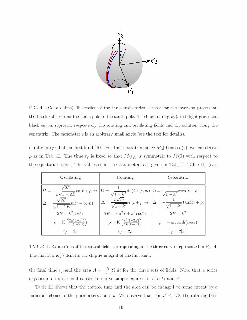
FIG. 4. (Color online) Illustration of the three trajectories selected for the inversion process on
the Bloch sphere from the north pole to the south pole. The blue (dark gray), red (light gray) and
black curves represent respectively the rotating and oscillating fields and the solution along the
separatrix. The parameter ǫ is an arbitrary small angle (see the text for details).
elliptic integral of the first kind [10]. For the separatrix, since M3(0) = cos(ǫ), we can derive
ρ as in Tab. II. The time tf is fixed so that ~M(tf ) is symmetric to ~M(0) with respect to
the equatorial plane. The values of all the parameters are given in Tab. II. Table III gives
Oscillating Rotating Separatrix
Ω = −√2E
k√1− 2E
cn(t+ ρ,m)
∆ =
√2E√
1− 2Esn(t+ ρ,m)
Ω =1√
1− k2dn(t+ ρ,m)
∆ =k√m√
1− k2sn(t+ ρ,m)
Ω =1√
1− k2sech(t+ ρ)
∆ = − 1√1− k2
tanh(t+ ρ)
2E = k2 cos2 ǫ 2E = sin2 ǫ+ k2 cos2 ǫ 2E = k2
ρ = K(
2E(1−k2)k2(1−2E)
)
ρ = K(
k2(1−2E)2E(1−k2)
)
ρ = −arctanh(cos ǫ)
tf = 2ρ tf = 2ρ tf = 2|ρ|.
TABLE II. Expressions of the control fields corresponding to the three curves represented in Fig. 4.
The function K(·) denotes the elliptic integral of the first kind.
the final time tf and the area A =∫ tf0
|Ω|dt for the three sets of fields. Note that a series
expansion around ε = 0 is used to derive simple expressions for tf and A.
Table III shows that the control time and the area can be changed to some extent by a
judicious choice of the parameters ε and k. We observe that, for k2 < 1/2, the rotating field
10

Oscillating Rotating Separatrix
tf = 2 ln(
4√1−k2ǫ
)
+O(ǫ2) tf = 2 ln(
4kǫ
)
+O(ǫ2) tf = 2 ln(
2ǫ
)
+O(ǫ2)
A = π√1−k2
− 2ǫ1−k2 +O(ǫ3) A = π√
1−k2A = π√
1−k2− 2ǫ√
1−k2+O(ǫ2).
TABLE III. Control time and area of the three families of fields for a small value of the parameter
ǫ.
allows us to make an inversion in a shorter time tf , but needs more energy. In contrast, the
oscillating mode offers the lowest energy and the shortest time if k2 > 3/4.
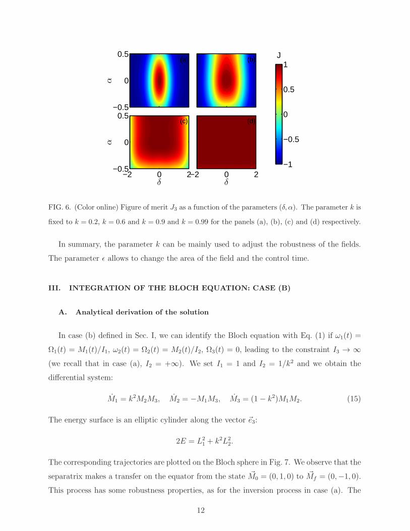
Another important feature of the control fields is their robustness property. Here, we
focus on the rotating solutions and the parameter ǫ is set to ǫ = 10−2. Figure 5 shows
different couples of fields (Ω,∆) for some values of k ∈ [0, 1]. The robustness is evaluated
0 0.5 10
20
40
60
80
100
t
Ω
k=0.01k=0.2k=0.6k=0.9k=0.99
0 0.5 1−100
−50
0
50
100
t
∆
k 0.01 0.2 0.6 0.9 0.99
Area (×π) 1.00 1.02 1.25 2.29 7.08
FIG. 5. Control fields computed for ǫ = 10−2 and for different values of k. The time has been
normalized to 1 from the scaling: t′ = t/tf , Ω′ = tf × Ω and ∆′ = tf ×∆.
with respect to a scaling factor α on the amplitude of the field and an arbitrary offset term,
δ, defined as follows:
Ω(α) = (1 + α)Ω, ∆(δ) = ∆+ δ.
We compute the figure of merit J3 = −M3(tf ) by propagating the system from ~M0 = (0, 0, 1)
through the Bloch equation of case (a) (see Sec. I). Figure 6 shows the efficiency of the
process as a function of the values of δ and α. A better robustness is achieved for larger
values of k.
11
α
(a)
−0.5
0
0.5(b)
α
δ
(c)
−2 0 2−0.5
0
0.5
δ
(d)
−2 0 2
J
−1
−0.5
0
0.5
1
FIG. 6. (Color online) Figure of merit J3 as a function of the parameters (δ, α). The parameter k is
fixed to k = 0.2, k = 0.6 and k = 0.9 and k = 0.99 for the panels (a), (b), (c) and (d) respectively.
In summary, the parameter k can be mainly used to adjust the robustness of the fields.
The parameter ǫ allows to change the area of the field and the control time.
III. INTEGRATION OF THE BLOCH EQUATION: CASE (B)
A. Analytical derivation of the solution
In case (b) defined in Sec. I, we can identify the Bloch equation with Eq. (1) if ω1(t) =
Ω1(t) = M1(t)/I1, ω2(t) = Ω2(t) = M2(t)/I2, Ω3(t) = 0, leading to the constraint I3 → ∞(we recall that in case (a), I2 = +∞). We set I1 = 1 and I2 = 1/k2 and we obtain the
differential system:
M1 = k2M2M3, M2 = −M1M3, M3 = (1− k2)M1M2. (15)
The energy surface is an elliptic cylinder along the vector ~e3:
2E = L21 + k2L2
2.
The corresponding trajectories are plotted on the Bloch sphere in Fig. 7. We observe that the
separatrix makes a transfer on the equator from the state ~M0 = (0, 1, 0) to ~Mf = (0,−1, 0).
This process has some robustness properties, as for the inversion process in case (a). The
12
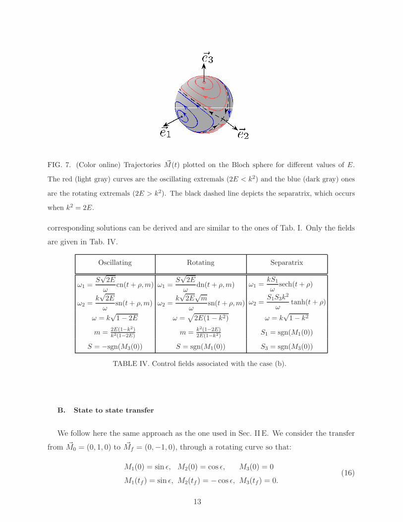
FIG. 7. (Color online) Trajectories ~M(t) plotted on the Bloch sphere for different values of E.
The red (light gray) curves are the oscillating extremals (2E < k2) and the blue (dark gray) ones
are the rotating extremals (2E > k2). The black dashed line depicts the separatrix, which occurs
when k2 = 2E.
corresponding solutions can be derived and are similar to the ones of Tab. I. Only the fields
are given in Tab. IV.
Oscillating Rotating Separatrix
ω1 =S√2E
ωcn(t+ ρ,m)
ω2 =k√2E
ωsn(t+ ρ,m)
ω1 =S√2E
ωdn(t+ ρ,m)
ω2 =k√2E
√m
ωsn(t+ ρ,m)
ω1 =kS1ω
sech(t+ ρ)
ω2 =S1S3k
2
ωtanh(t+ ρ)
ω = k√1− 2E ω =
√
2E(1 − k2) ω = k√1− k2
m = 2E(1−k2)k2(1−2E)
m = k2(1−2E)2E(1−k2) S1 = sgn(M1(0))
S = −sgn(M3(0)) S = sgn(M1(0)) S3 = sgn(M3(0))
TABLE IV. Control fields associated with the case (b).
B. State to state transfer
We follow here the same approach as the one used in Sec. II E. We consider the transfer
from ~M0 = (0, 1, 0) to ~Mf = (0,−1, 0), through a rotating curve so that:
M1(0) = sin ǫ, M2(0) = cos ǫ, M3(0) = 0
M1(tf ) = sin ǫ, M2(tf ) = − cos ǫ, M3(tf ) = 0.(16)
13

The fields can be expressed as follows:
ω1 =1√
1− k2dn(t+ ρ), ω2 =
k√m√
1− k2sn(t+ ρ),
2E = sin2 ǫ+ k2 cos2 ǫ, ρ = K(m), tf = 2ρ,
(17)
with m given in Tab. IV. We set ǫ = 10−2 and we investigate the robustness properties. In
this case, the Bloch equation reads:
~M =
0 −δ (1 + α)ω2
δ 0 −(1 + α)ω1
−(1 + α)ω2 (1 + α)ω1 0
~M. (18)
We consider different control fields for different values of k and we evaluate their robustness
as a function of δ and α. The results are shown in Fig. 8.
α
(a)
−0.5
0
0.5(b)
α
δ
(c)
−2 0 2−0.5
0
0.5
δ
(d)
−2 0 2
J
−1
−0.5
0
0.5
1
FIG. 8. (Color online) Figure of merit J2 = −M2(tf ) as a function of the parameters (δ, α). The
parameter k is respectively fixed to k = 0.2, k = 0.7, k = 0.9 and k = 0.99 for the panels (a), (b),
(c) and (d). In each case, the parameter ǫ is set to 10−2.
C. Global phase
The Bloch vector ~M(t) does not take into account the global phase of the quantum state.
We show for the case (b) how to derive this phase by introducing the Euler angles, which
completes the analogy between the two-level quantum system and the classical rigid body.
14

We introduce three Euler angles θ, φ and ψ as shown in Fig. 9. The two angles θ and φ
define the position of the vector ~M , and the motion of the frame ( ~Q, ~P , ~M) with respect to
the fixed one (~e1, ~e2, ~e3) can be described with the third Euler angle ψ.
~P
N
ψ
~e2
φ
~Q
~e3
θ~M
~e1
FIG. 9. (Color online) Definition of Euler angles from the frame attached to the Bloch sphere
(~e1, ~e2, ~e3). In a classical system, (~e1, ~e2, ~e3) is the frame attached to the rigid body. The vector ~M
plays the role of the angular momentum ~L of the fictitious rigid body.
The set of angles θ, φ and ψ can be used to parameterize the wave function |λ(t)〉 as:
|λ〉 =
cos(
θ2
)
e−iφ
2
sin(
θ2
)
eiφ
2
e−iψ
2 . (19)
The dynamics of the three angles can be obtained by substituting Eq. (19) into the
Schrodinger equation (6). We arrive at:
θ = ω2 cosφ− ω1 sinφ
φ = −ω1cosφtan θ
− ω2sinφtan θ
ψ = ω1cosφsin θ
+ ω2sinφsin θ
.
(20)
In the Bloch representation, the two angles θ and φ define the vector ~M(t) such that:
M1 = sin θ cosφ, M2 = sin θ sinφ, M3 = cos θ. (21)
The two control fields can be expressed in terms of the Euler angles as follows:
ω1 =1ωsin θ cosφ, ω2 =
k2
ωsin θ sinφ.
15

The final dynamical system to solve can be written as:
θ = −1−k2
ωsin θ cosφ sinφ
φ = − 1ωcos θ(cos2 φ+ k2 sin2 φ)
ψ = 1ω
(
cos2 φ+ k2 sin2 φ)
.
(22)
D. Rotation matrix
We introduce a 3 × 3 matrix R defined by R(t) = ( ~Q(t), ~P (t), ~M(t)), and we denote by
Rf the final propagator which satisfies R(tf ) = RfR(0). The propagator Rf is given by:
Rf = R(tf )tR(0).
The matrix R can be written as a function of the Euler angles, R = RφRθRψ with:
Rφ =
cosφ − sinφ 0
sinφ cosφ 0
0 0 1
, Rθ =
cos θ 0 sin θ
0 1 0
− sin θ 0 cos θ
, Rψ =
cosψ − sinψ 0
sinψ cosψ 0
0 0 1
. (23)
We introduce the angles (θ0, φ0, ψ0) and (θf , φf , ψf ), which are respectively the initial and
final values of the Euler angles. The initial global phase ψ0 is irrelevant, and can be set to
0 without loss of generality.
For a trajectory such that: θf = θ0 = π/2, φf = −φ0, ψf = (2n + 1)π and ψ0 = 0, the
final rotation matrix becomes:
Rf =
1 0 0
0 −1 0
0 0 −1
.
Note that this matrix is also the one realized after the application of a π pulse along ~e1.
We will see in the next section that for ψf = 3π (n = 1), the dynamics of this process is
associated with the tennis racket effect [7]. This effect is described in Sec. IV.
IV. THE CLASSICAL AND THE QUANTUM TENNIS RACKET EFFECTS
The classical tennis racket effect (TRE) is a particular motion which occurs for some
trajectories in the neighbourhood of the separatrix [7]. We recall that, for a classical rigid
16

body, ~e1, ~e2 and ~e3 are the principal axes of inertia of the solid. If the principal moments of
inertia are such that I1 < I2 < I3 (it is the used convention in this work) then a rotation
about the ~e1- and ~e3- axes is stable, but a rotation about ~e2 is unstable. This point can be
checked in Fig. 7.
The TRE is easier to figure out by considering the classical case, where ( ~X, ~Y , ~L) is
the laboratory frame and (~e1, ~e2, ~e3) is the frame attached to the racket [7, 8]. In this
representation, ~e1 is along the handle, ~e2 is perpendicular to the handle and belongs to
the head of the racket, and ~e3 is perpendicular to the head. The corresponding process is
displayed in Fig. 10.
~L
~e2
~e3~Y ≡
~e1~X
~e3
~e2~L
~Y
~e1~X
FIG. 10. Illustration of the initial conditions (left), and final conditions (right) of the classical
tennis racket effect. The vector ~L is the classical angular momentum of the racket. Note that ~e1
and ~e2 are not exactly collinear to ~X and ~L.
For a standard tennis racket, this process occurs for trajectories starting in the neigh-
bourhood of the unstable equilibrium point, i.e. ~L ≃ ~e2 at time t = 0. Note that if we apply
two times this motion then the racket goes back to its initial position. In other words, if we
consider the frame S = (~e1, ~e2, ~e3), we have:
S(0) 1 TRE−→
1 0 0
0 −1 0
0 0 −1
S(0) 2 TRE−→ S(0). (24)
We have now all the tools in hand to describe the quantum TRE. In the (θ,φ,ψ)- represen-
17

k 0.2 0.4 0.6 0.7 0.9
π2 − φ0 1.55 × 10⁻⁷ 4.66 × 10⁻⁴ 1.54× 10⁻² 5.18 × 10⁻² 0.531
TABLE V. Values of the initial angle φ0 as a function of the parameter k (see the text for details).
tation, the TRE satisfies:
ψ0 = 0, ψf = 3π, θf = θ0 = π/2, φf = −φ0. (25)
If we substitute these relations into the wave function of Eq. (19), we obtain that the wave
function goes back to its initial state after the application of four TRE, i.e.
|λ0〉 1 TRE−→
0 −i−i 0
|λ0〉 2 TRE−→
−1 0
0 −1
|λ0〉 3 TRE−→
0 i
i 0
|λ0〉 4 TRE−→ |ζ0〉.
Among all the possible trajectories, only one exactly satisfies the quantum TRE process of
Eq. (25). Since θ0 = π/2, we can deduce from Fig. 7 that this curve is a rotating one, starting
and ending in the (~e1, ~e2)- plane. Unfortunately, the initial conditions of this trajectory are
difficult to compute analytically, because the phase ψ can only be expressed in terms of
elliptic integrals of the first and third kinds. We thus give directly the numerical values
of the coordinates of the initial point for different values of k in Tab. V. Since θ0 = π/2
and ψ0 = 0, only the initial value of φ0 is needed. A TRE is obtained if the trajectory of
~L(t) is close to the separatrix of Fig. 7, which means that ~L(0) starts close to the unstable
equilibrium point (0, 1, 0), or equivalently that the initial value of φ is of the order of π/2.
The corresponding fields are given by:
ω1 =1√
1− k2dn(t+ ρ), ω2 =
k√m√
1− k2sn(t+ ρ),
2E = cos2 φ0 + k2 sin2 φ0, ρ = K(m), tf = 2ρ.
(26)
We now apply this set of control fields to the quantum system, in order to implement the
quantum tennis racket effect. The control process is a unitary transformation which does
not depend on the initial conditions. We consider the following initial point:
~Q(0) = ~e3, ~P (0) = ~e1, ~M(0) = ~e2. (27)
The TRE-pulse makes a global rotation about the axis ~e1. The three states are given at
time tf by:
~Q(tf) = −~Q(0), ~P (tf ) = ~P (0), ~M(tf ) = − ~M(0). (28)
18

We consider the case k = 0.7. The control fields are computed from Eq. (26). The dynamics
of the vectors ~Q, ~P and ~M are plotted in Fig. 11. We also represent in Fig. 11 the motion
of the vectors ~e1, ~e2 and ~e3 in the ( ~Q, ~P , ~M)- frame, which is more suitable to describe the
classical TRE (in the classical problem, (~e1,~e2,~e3) is the frame attached to the racket).
0 5 10 15−1
−0.5
0
0.5
1
t
Am
plitu
de
Q1
Q2
Q3
0 5 10 15t
P1
P2
P3
0 5 10 15t
M1
M2
M3
FIG. 11. (Color online) Upper panels: Evolution of the coordinates of ~Q (left), ~P (middle) and
~M (right) as a function of time, for k = 0.7. The coordinates of the vectors ~M , ~P and ~Q are
denoted by (M1,M2,M3), (P1, P2, P3) and (Q1, Q2, Q3), respectively. Lower left panel: Evolution
of ~Q (green- light gray), ~P (red- dark gray) and ~M (blue- black) on the Bloch sphere. Lower
right panel: Motion of ~e1 (blue- black), ~e2 (red- dark gray) and ~e3 (green- light gray) in the frame
( ~Q, ~P , ~M). This dynamics corresponds to the one of the quantum tennis racket effect, where the
dynamics of ~M is similar to the dynamics of the classical angular momentum.
V. IMPLEMENTATION OF QUANTUM GATES
The goal of this section is to show how the dynamics of a rigid body can be used to
implement one-qubit quantum gates. In Sec. VA, we consider the example of the Hadamard
19

gate before generalizing this result to any one-qubit quantum gate in Sec. VB. Section VC
is dedicated to the case of geometric phase gates. The robustness issue of the gates with
respect to experimental imperfections is investigated in Sec. VD. Generalizing the BIR
approach used in NMR [27, 28], we show that the quantum gates can be made robust.
As an illustrative example, we consider the case of a NOT gate and its robustness against
control field inhomogeneities.
A. The Hadamard gate
The Hadamard gate UH is a unitary transformation which can be decomposed into a π
phase gate and a π2rotation gate. It reads:
UH = − i√2
1 1
1 −1
. (29)
We can show that this gate corresponds to a transformation GH in SO(3):
GH =
0 0 1
0 −1 0
1 0 0
. (30)
In a classical rigid body, the Hadamard gate realizes the following transfer:
R(0) → R(tf ) = GHR(0), (31)
where R is the rotation matrix given in terms of Euler’s angles. Since the classical angular
momentum ~L must also satisfy the transfer (31), we deduce that:
L1(tf ) = L3(0), L2(tf ) = −L2(0), L3(tf) = L1(0). (32)
We choose a trajectory such that L1(0) = L3(0) and L1(tf) = L3(tf) at time tf , which
ensures that the Hadamard transformation is satisfied for ~L, due to the symmetries of the
Jacobi functions. These conditions can be verified for a rotating extremal if k < 1/√2, an
oscillating one if k > 1/√2 and along the separatrix if k = 1/
√2. As an illustrative example,
we set k = 0.5. The solution is a rotating extremal of the form:
L1(t) =√2E dn(t+ ρ,m),
L2(t) = −√2Emk
sn(t + ρ,m),
L3(t) =√1− 2E cn(t + ρ,m).
(33)
20

It can be shown that the initial condition L1(0) = L3(0) implies that the parameter ρ is
given by:
ρ = −F
[√
m(1− k2)− k2
m(1− 2k2), m
]
. (34)
The condition at time tf is satisfied if we choose tf such that:
tf = 2|ρ|. (35)
Equations (34) and (35) ensure that ~L satisfies the conditions of the Hadamard gate. How-
ever, another relation is required on the global phase of the state. It is given by the final
value of the euler angle ψ(tf ) (we recall that at time t = 0, we can set ψ(0) = 0). Using the
relations
L1 = sin θ cosφ, L2 = sin θ sinφ, L3 = cos θ, (36)
we obtain that θ(tf ) = θ(0) and φ(tf) = −φ(0). Moreover, since the rotation matrix R can
be written as R = RφRθRψ, where Rφ, Rθ and Rψ are defined in Eq. (23), straightforward
computations lead to the following global phase ψ(tf ):
tanψ(tf) =
√
(
L2(0)
L1(0)
)4
+ 2
(
L2(0)
L1(0)
)2
. (37)
The Hadamard gate is associated with a trajectory of the rigid body satisfying Eqs. (34), (35)
and (37). However, the global phase ψ can only be expressed in terms of elliptic integrals
of the third kind. A numerical solution for k = 0.5 is given by the following initial angular
momentum:
L1(0) = 0.1331, L2(0) = 0.9821, L3(0) = L1(0). (38)
The corresponding trajectories of the frames ( ~X, ~Y , ~L) and ( ~Q, ~P , ~M) of the classical and
quantum systems are displayed in Fig. 12.
B. Generalization to any one-qubit gate
The goal of this paragraph is to show that the trajectories of the free rotation of a rigid
body allow us to realize any one-qubit gate. We first present a proof showing that the
reachable set of the control protocol is SO(3) and then a numerical method that can be
applied for any gate.
21

FIG. 12. (Color online) Left panel: Hadamard gate in the classical system. Right panel: Hadamard
gate in the quantum system. In this case, at time t = 0, we have ~Q(0) ≡ ~e1, ~P (0) ≡ ~e2, ~M(0) ≡ ~e3.
The rotation matrix R(t) associated with the classical system can be viewed as the optimal
solution of the following dynamical system:
R =
0 0 ku2
0 0 −u1−ku2 u1 0
R, (39)
with the constraint u21 + u22 = 1. Note that this system is fully controllable, which means
that any rotation matrix R can be realized.
We denote by aij the element of the ith row and jth column of the matrix R. We introduce
~r the vector defined as ~r = t(a11, a21, · · · , a33), and we define the energy minimum pseudo-
Hamiltonian Hp of the Pontryagin Maximum Principle (See Ref. [14] for mathematical
details):
Hp = ~p · ~r − 12
(
u21 + u22)
, (40)
where ~p = t(b11, b21, · · · , b33) is the adjoint state vector. We define the following angular
momentum:
~L =
L1
L2
L3
=3
∑
n=1
b1n
b2n
b3n
×
a1n
a2n
a3n
. (41)
The pseudo-Hamiltonian can be written in terms of the component of this angular momen-
22

tum as:
Hp = u1L1 + ku2L2 − 12
(
u21 + u22)
. (42)
The Pontryagin Maximum Principle states that the dynamics and the associated control
fields are optimal if this pseudo-Hamiltonian is maximum. The Pontryagin Hamiltonian His defined so that H = maxu2
1+u2
2=1Hp. This optimality condition is satisfied for the following
control fields u1 =L1√
L21+k2L2
2
and u2 =kL2√L21+k2L2
2
. In this case, we get that 2E = L21 + k2L2
2
is constant and we can show that the dynamics of the angular momentum ~L satisfies the
Euler’s equation (15).
In order to illustrate the fact that any gate can be realized, we propose a numerical
method to obtain the following gate:
Rf =1
4
−√62
−3√6
21
5√2
2−
√22
√3
−√2
√2 2
√3
. (43)
We define the function F = 13Trace[tRf · (R(t) · tR(0))], where R(t) is the rotation matrix
associated with the classical system. We recall that the product R(t) · tR(0) gives the value
of the gate realized by the classical system at time t. We fix a maximum value for the time
Tmax = 4K(m) which corresponds to a complete revolution of ~L(t), and we integrate the
system (22) numerically from t = 0 to t = Tmax for different initial points (θ(0), φ(0)). We
determine numerically the value F ∗ for which F is maximum, and the corresponding time
T ∗. We then plot F ∗ as a function of θ(0) and φ(0). The result is displayed in Fig. 13 for
k = 0.5. This analysis allows us to determine the initial point (θ(0), φ(0)) and the final time
tf = T ∗ of the gate. We obtain:
θ(0) = 0.7104, φ(0) = −0.6078, tf = 6.543, (44)
for k = 0.5.
C. Geometric phase gate
The free rotation of a rigid body has a geometric feature called the Montgomery phase [15,
16]. This phase can be defined by considering one period of the angular momentum ~M in
the frame (~e1, ~e2, ~e3). During this motion, the frame ( ~Q, ~P , ~M) rotates about ~M by an angle
23

φ(0)
θ(0
)
−1 0 10
0.5
1
1.5
F ∗
0.2
0.3
0.4
0.5
0.6
0.7
0.8
0.9
φ(0)
θ(0
)
−1 0 10
0.5
1
1.5
T ∗
0
1
2
3
4
5
6
7
FIG. 13. (Color online) Evolution of F ∗ as a function of (θ(0), φ(0)) (left), and of the corresponding
time T ∗ (right) for k = 0.5. The cross depicts the point (θ(0), φ(0)) for which the gate is realized
with a precision of 1−F ∗ = 1.69× 10⁻⁵. Note that this solution is not unique. We choose the one
with the shortest time transfer.
∆ψ (see Fig. 9), which is the Montgomery phase. This phase can be expressed as the sum
of a dynamical and a geometric parts as follows:
∆ψ =2ET
M− S,
where M is the norm of the angular momentum, T the period of the motion of ~M and S is
the solid angle swept out by the angular momentum vector in the frame (~e1, ~e2, ~e3). Starting
from the conservation of the energy 2E =M21 + k2M2
2 , and using Eq. (22) we have:
2E = sin2 θ(cos2 φ+ k2 sin2 φ) = ω(1− cos2 θ)ψ. (45)
From cos2 θψ = − cos θφ, we get:
dψ =2E
ωdt− cos θdφ =
2E
ωdt−
(∫ θ
π/2
sin θ′dθ′)
dφ. (46)
Thus, the variation ∆ψ of the phase for one period is given by:
∆ψ =2ET
ω− S, (47)
where S =∫ φfφ0
∫ θ(φ)
π/2sin θdθdφ is the solid angle swept out by ~M . This formula is of the same
form as the well-known Berry phase [17, 18] in quantum mechanics which can be used for
24

adiabatic [18] and periodic [19] trajectories on the Bloch sphere. Such geometric phases have
been recently the subject of a large interest in quantum computing as a way to implement
geometric and thus robust quantum gates [20, 21]. One of the main difficulties to implement
phase gates using geometric phases is to find a way to cancel the dynamical contribution of
the phase. Different techniques have been proposed up to date [20, 21]. For instance, Jones
et al. [22] showed that the dynamical part of Berry’s phase can be removed by using two
cyclic trajectories of ~M(t) on the Bloch sphere, the second cycle being surrounded by a pair
of π pulses. In [22], the geometric phase gate was implemented in the adiabatic regime, but
it is possible to generalize this process to consider non-adiabatic cyclic evolution [23–26].
We propose here a method based on the free rotation of a rigid body and the TRE to
implement a geometric phase gate in the non-adiabatic regime. We first recall that each
trajectory ~M(t) of Fig. 7 can evolve in the backward direction by changing the sign of
the control field ω1(t) (see Sec. I). If we consider two identical cycles, the second being
followed in the backward direction along the same trajectory, then all the phases vanish, the
dynamical ones as well as the geometric ones. However, if for the second cycle, the value
of k is different from the first cycle, the total phase at the end of the process is given by
∆ψcycle 1 −∆ψcycle 2. This process does not cancel automatically the dynamical phases. To
do so, a particular trajectory for the second cycle has to be chosen.
The method can be described as follows. To simplify the discussion and the analytical
computations, we assume here that the system follows trajectories along the separatrices. A
similar process can be designed by considering trajectories associated with the TRE, which
are close to the separatrices. More precisely, we first make a transfer along the separatrix
from the point (0, 1, 0) to the point (0,−1, 0) with a finite (long enough) time, and a fixed
value ka. The second step consists in bringing the system from (0,−1, 0) to (0, 1, 0) also
along the separatrix but with a different value of the parameter k, i.e. kb 6= ka. Since the
time Tb of the second process can be chosen arbitrarily long, we choose Tb such that the two
dynamical phases cancel each other. The global process is shown in Fig. 14 and described
in Tab. VI.
In order to derive the geometric phase, we consider the case of a separatrix such that
M1(t) > 0 and M3(t) > 0 for t > 0. We start from the following expression of the geometric
25

phase:
S =
∫ π/2
−π/2
∫ θ(φ)
π/2
sin θdθdφ = −∫ π/2
−π/2cos θ(φ)dφ. (48)
For this separatrix, we have θ ∈ [0, π/2], which gives cos θ =√
1− sin2 θ. Along the
separatrix, 2E = k2 and we can express sin2 θ in terms of the angle φ using Eq. (45). We
deduce that:
S = −∫ π/2
−π/2
√
1− k2 − (1− k2) sin2 φ
1− (1− k2) sin2 φ= −
∫ π/2
−π/2
√1− k2
cosφ√
cos2 φ+ k2 sin2 φ. (49)
Finally, the integration gives:
S = −2 arcsin(√1− k2). (50)
We recall that the system evolves in the forward and backward directions for the cycles (a)
and (b), respectively. Moreover, on the separatrix we have ω = k√1− k2 and 2E = k2.
Thus, for each cycle, the variation ∆ψ is given by:
∆ψa =kaTa
√
1− k2a+ 2 arcsin(
√
1− k2a), ∆ψb = − kbTb√
1− k2b− 2 arcsin(
√
1− k2b ). (51)
If we choose Tb such that:
Tb =ka√
1− k2bkb√
1− k2aTa, (52)
then the two dynamical phases cancel each other and we get a purely geometric phase given
by:
∆ψtot = ∆ψa +∆ψb = 2[arcsin(√
1− k2a)− arcsin(√
1− k2b )]. (53)
Going back to the expression of the quantum state of Eq. (19), this corresponds to a phase
gate of the form
1 0
0 ei∆ψtot
. (54)
The global process with the applied control fields is described in Tab. VI. The final geo-
metric phase is equal to the area displayed in Fig. 14. In Fig. 14, we consider the following
parameters Ta = 100, ka = (√
2−√2)/2 and kb = (
√
2 +√2)/2 in order to implement a
geometric phase equal to ∆ψtot = π/2.
26

Path a Path b
t ∈ [0, Ta] t ∈ [Ta, Ta + Tb]
Ta long enough Tb =ka√
1−k2b
kb√
1−k2aTa
ω1(t) =1√1−k2a
sech(t+ ρa) ω1(t) = − 1√1−k2
b
sech(t+ ρb)
ω2(t) = − 1
ka√
1−k2atanh(t+ ρa) ω2(t) = − 1
kb√
1−k2b
tanh(t+ ρb)
ρa = −Ta/2 ρb = −Tb/2− Ta.
TABLE VI. Description of the process for implementing a phase gate. Note that the sign of ω1
changes in the cycle (b) in order to follow the second trajectory in the backward direction.
FIG. 14. (Color online) Trajectories on the Bloch sphere for implementing a π/2 phase gate. The
brown (gray) surface is the total geometric phase at the end of the process i.e. Stot = π/2.
D. Robustness of the NOT gate
We show in this paragraph how the robustness of the control fields used to implement
one-qubit gates can be improved. The approach is inspired from the BIR- pulses method in
NMR [27, 28]. We design a pulse which allows us to realize a NOT gate in a robust manner
with respect to the control fields- inhomogeneities, which is equivalent to a BIR-1 pulse in
the adiabatic limit [27, 28]. We use the fact that the global phase of the state monotonically
increases or decreases when the system follows a specific trajectory of the phase portrait.
This property allows us to cancel the global phase of the dynamics (both dynamical and
geometrical terms) and then to realize a robust NOT gate. As an example, we consider here
the separatrix of the configuration (a) (see Fig. 2).
27

The separatrix is first followed from the north pole to the equatorial plane of the sphere in
the direction given in Fig. 2. We then transfer the state to another separatrix followed in the
opposite direction in order to reach the south pole of the Bloch sphere. The two separatrices
are connected with a constant pulse ∆(t) about ~e3. The global phase is cancelled leading to
an inversion with a phase equal to zero, i.e. a NOT- gate along the ~e2- axis. The trajectory is
represented in Fig. 15. We can show that the azimuthal angle between the two separatrices
FIG. 15. (Color online) Trajectory used to realized a NOT- gate (solid blue line). The dashed lines
represent the separatrices. The black arrows indicate the direction of the dynamics of the classical
angular momentum.
is equal to 2 arccos k. We thus need to apply a 2 arccos k- pulse along ~e3 when the Bloch
vector belongs to the equator. Note that in the adiabatic limit, which corresponds here to
k → 1, this angle tends to zero. In the latter case, the method is equivalent to a 180 BIR-1
pulse [27], with an Allen-Eberly hyperbolic shape. The details of the pulse are given in
Tab. VII. The robustness of the control process is shown in Fig. 16 for a control field of the
t ∈[
0, T2 − T∆2
]
t ∈[
T2 − T∆
2 ,T2 + T∆
2
]
t ∈[
T2 + T∆
2 , T]
Ω = 1√1−k2
sech(t+ ρ) Ω = 0 Ω = − 1√1−k2
sech(t+ ρ)
∆ = − k√1−k2
tanh(t+ ρ) ∆ = 2arccos(k)T∆
∆ = k√1−k2
tanh(t+ ρ)
ρ = −T−T∆2 ρ = −T+T∆
2
TABLE VII. Details of the pulse used to implement robust- NOT gates. T is the total duration of
the process and T∆ is the duration of the constant pulse along ~e3.
form:
Ω(α) = (1 + α)Ω,∆(α) = ∆, (55)
28

where α is a scaling factor corresponding to the fields inhomogeneities. The fidelity J is
defined such that J = Trace(tR(tf ) · Rf), where Rf is the target rotation matrix given by:
Rf =
−1 0 0
0 1 0
0 0 −1
. (56)
The fidelity has been also computed for a standard π- pulse and for the TRE- pulse adapted
to configuration (a) in order to compare the three methods.
−0.5 0 0.5−0.5
0
0.5
1
α
J
π−pulseTRERobust
FIG. 16. (Color online) Robustness of the NOT gate implemented with a standard π- pulse (blue
or black), a TRE- pulse (green or light gray), and with the method detailed above (red of dark
gray), for k = 0.9. The robustness of the method can be improved by choosing k closer to 1.
VI. NUMERICAL IMPLEMENTATION OF THE TRAJECTORIES OF A RIGID
BODY AND OF A CONTROL PULSE SEQUENCE
We provide in this supplementary material a Matlab code to compute the trajectories of
a rigid body as a function of the parameters k and E. We also deduce the associated control
fields and the dynamics of the Bloch vector for a state to state transfer. This code can be
used by the interested reader to test some of the control protocols proposed in this work.
VII. JACOBI’S ELLIPTIC FUNCTIONS
We recall in this paragraph some standard properties of Jacobi’s elliptic functions used in
this paper [10]. Jacobi’s elliptic functions generalize the standard trigonometric functions.
29

This is a family of functions which includes cosine, sine and hyperbolic functions. They
are written as follows: sn(u,m), cn(u,m) and dn(u,m). Their periods are related to the
complete elliptic integral of the first kind K(m) as 4K(m), 4K(m) and 2K(m), respectively,
with m a parameter belonging to the interval [0, 1]. The elliptic integral is defined as:
K(m) =
∫ 1
0
dx√1− x2
√1−mx2
.
In the case m = 0, we have K(m) = π/2 and the functions sn(u,m), cn(u,m) and dn(u,m)
become sin(u), cos(u) and 1, respectively. In the case m = 1, we obtain K(m) = +∞ and
the elliptic functions can be identified with tanh(u), sech(u) and sech(u). For a value of m
such that m = 1 − ε with ε a small positive parameter, the function K(m) is, to the first
order, given by:
K(1− ǫ) =1
2ln
(
8
ε
)
+O(ε). (57)
Figure 17 shows Jacobi’s elliptic functions for m = 1/2.
0 K 2K 3K 4K
−1
0
1
u
Am
plitu
de
cn
sn
dn
u 0 K(m) 2K(m) 3K(m)
sn(u,m) 0 1 0 -1
cn(u,m) 1 0 -1 0
dn(u,m) 1√1−m 1
√1−m
FIG. 17. (Color online) Plot of Jacobi’s Elliptic functions in terms of u for m = 1/2. The Table
gives some particular values of the same functions.
These functions satisfy the following relations:
sn2(u,m) + cn2(u,m) = 1,
m sn2(u,m) + dn2(u,m) = 1.
30

Primitive Function Derivative
1√mln(
dn(u,m) −√m cn(u,m)
)
sn(u,m) cn(u,m)dn(u,m)
1√marctan
(√m sn(u,m)dn(u,m)
)
cn(u,m) −sn(u,m)dn(u,m)
am(u,m) dn(u,m) −msn(u,m)cn(u,m)
TABLE VIII. Derivatives and primitives of the Jacobi’s elliptic functions.
The derivatives and the primitives of sn, cn and dn are given in Tab. VIII.
[1] L. D. Landau and E. M. Lifshitz, Mechanics (Pergamon Press, Oxford, 1960).
[2] H. Goldstein, Classical Mechanics (Addison-Wesley, Reading M. A., 1950).
[3] M. H. Levitt, Spin Dynamics: Basics of Nuclear Magnetic Resonance (Wiley, New York,
2008).
[4] R. R. Ernst, G. Bodenhausen and A. Wokaun, Principles of Nuclear Magnetic Resonance in
One and Two Dimensions (Oxford Science Publications, 2004).
[5] D. Daems, A. Ruschhaupt, D. Sugny and S. Gurin, Robust Control by a Single-Shot Shaped
Pulse, Phys. Rev. Lett. 111, 050404 (2013)
[6] L. Allen and J. H. Eberly, Optical Resonance and Two-Level Atoms, (Wiley, New York, 1975).
[7] L. Van Damme, P. Pavao Mardesic and D. Sugny, The tennis racket effect in a three-
dimensional rigid body, Physica D 338, 17 (2017)
[8] M. S. Ashbaugh, C. C. Chiconc and R. H. Cushman, The twisting tennis racket, J. Dyn. Diff.
Eq. 3, 67 (1991)
[9] N. V. Vitanov, T. Halfman, B. W. Shore and K. Bergmann, Laser-induced population transfer
by adiabatic passage techniques, Annu. Rev. Phys. Chem. 52, 763 (2001)
[10] M. Abramowitz, Handbook of Mathematical Functions, (Dover Publications, New York, 1964).
[11] K.-A. Suominen and B. M. Garraway, Population transfer in a level-crossing model with two
time scales, Phys. Rev. A 45, 1 (1992)
[12] F. T. Hioe and C. E. Carroll, Two-state problems involving arbitrary amplitude and frequency
modulations, Phys. Rev. A 32, 1541 (1985)
[13] F. T. Hioe, Solution of Bloch equations involving amplitude and frequency modulations, Phys.
31

Rev. A 30, 2100 (1984)
[14] B. Bonnard and D. Sugny, Optimal control with applications in space and quantum dynamics,
AIMS: Applied mathematics Vol. 5 (2012).
[15] R. Montgomery, How much does the body rotate? A Berry’s phase from the 18th century, Am.
J. Phys. 59, 394 (1991)
[16] J. Natario, An elementary derivation of the Montgomery phase formula for the Euler top, J.
Geom. Mech. 2, 113 (2010)
[17] A. Bohm, A. Mostafazadeh, H. Koizumi, Q. Niu and J. Zwanziger, The geometric phase in
quantum systems, Springer (2003)
[18] M. V. Berry, Quantal phase factors accompanying adiabatic changes, Proc. Roy. Soc. London,
Ser. A 392, 45 (1984)
[19] Y. Aharanov and J. Anandan, Phase change during a cyclic quantum evolution, Phys. Rev.
Lett. 58, 1593 (1987)
[20] E. Sjoqvist, A new phase in quantum computation, Physics, 1, 35 (2008)
[21] A. Ekert, M. Ericsson, P. Hayden, H. Inamori, J. A. Jones, D. K. L. Oi and V. Vedral,
Geometric quantum computation, J. Mod. Opt. 47, 2501 (2000)
[22] J. A. Jones, V. Vedral, A. Eckert and G. Castagnoli, Geometric quantum computation with
NMR, Nature 403, 869 (2000).
[23] W. Xiand-Bin and M. Keiji, Nonadiabatic conditional geometric phase shift with NMR, Phys.
Rev. Lett. 87, 097901 (2001)
[24] S.-L. Zhu and Z. D. Wang, Implementation of univeral quantum gates based on nonadiabatic
geometric phases, Phys. Rev. Lett. 89, 097902 (2002)
[25] Y. Ota, Y. Goto, Y. Kondo and M. Nakahara, Geometric quantum gates in liquid state NMR
based on a cancellation of dynamical phases, Phys. Rev. A 80, 052311 (2009)
[26] S. L. Zhu and Z. D. Wang, Universal quantum gates based on a pair of orthogonal cyclic states:
Application to NMR systems, Phys. Rev. A 67, 022319 (2003)
[27] A. Tannus and M. Garwood, Adiabatic pulses, NMR Biomed 10, 423 (1997)
[28] M. Garwood and Y. Ke, Symmetric pulses to induce arbitrary flip angles with compensation
for RF inhomogeneity and resonance offsets, J. Magn. Reson. 94, 511 (1991)
32

clear all
close all
clc
%%%%%%%%%%%%%%%%%%%%%%%%%%%%%%%%%%%%%%%%%%%%%%%%%%%%%%%%%%%%%
%Choose a set of parameters k,E
k=0.7;
E=0.25;
%The separatrix is given for E=k^22
%%%%%%%%%%%%%%%%%%%%%%%%%%%%%%%%%%%%%%%%%%%%%%%%%%%%%%%%%%%%%
%Compute the parameters of elliptic functions
if 2*E < k^2 %Oscillating
w = k*sqrt1-2*E;
m = 2*E*1-k^2k^2*1-2*E; %Ellipticity
rho = ellipke(m); %Initial phase
tf = 2*rho; %Final time=12 period
elseif 2*E > k^2 %Rotating
w = sqrt2*E*1-k^2;
m = k^2*1-2*E2*E*1-k^2;
rho = ellipke(m);
tf = 2*rho;
elseif 2*E == k^2 %Separatrix
w = k*sqrt1-k^2;
rho = -10;
tf = 2*absrho;
end
%Define the numerical control time
N=1000;
t=linspace0,tf,N;
%%%%%%%%%%%%%%%%%%%%%%%%%%%%%%%%%%%%%%%%%%%%%%%%%%%%%%%%%%%%%
%Control fields and angular momentum
if 2*E < k^2 %Oscillating trajectory
%Compute the elliptic function cn sn dn
[sn cn dn]=ellipjt+rho,m;
%Control fields
w1 = -sqrt2*Ew*cn;
w2 = k*sqrt2*Ew*sn;
%Angular momentum
L1 = -sqrt2*E*cn;
L2 = sqrt2*Ek*sn;
L3 = wk*dn;
elseif 2*E > k^2 %Rotating trajectory
%Compute the elliptic function cn sn dn
[sn cn dn]=ellipjt+rho,m;
%Control fields
w1 = sqrt2*Ew*dn;
w2 = k*sqrt2*E*sqrt(m)/w*sn;
%Angular momentum
L1 = sqrt2*E*dn;
L2 = sqrt2*m*Ek*sn;
L3 = -w*sqrt(m)k*cn;
elseif 2*E == k^2 %Separatrix
%Control fields
w1 = kw*secht+rho;

w2 = k^2w*tanht+rho;
%Angular momentum
L1 = k*secht+rho;
L2 = tanht+rho;
L3 = wk*secht+rho;
end
%%%%%%%%%%%%%%%%%%%%%%%%%%%%%%%%%%%%%%%%%%%%%%%%%%%%%%%%%%%%%
%Integration of the Bloch equation
%Basis
Sx=[0 0 0;0 0 -1;0 1 0];
Sy=[0 0 1;0 0 0;-1 0 0];
%State tabular
M=zeros3,N+1;
M:,1=[0;1;0]; %Example of initial state: y-axis of the Bloch sphere
dt=t2-t1;
%Propagation
for n=1:N
H=w1(n)*Sx+w2(n)*Sy; %Propagator
M:,n+1=expmH*dt*M(:,n);
end
M1=M1,:;
M2=M2,:;
M3=M3,:;
tM=linspace0,tf,N+1; %Time of length N+1
%%%%%%%%%%%%%%%%%%%%%%%%%%%%%%%%%%%%%%%%%%%%%%%%%%%%%%%%%%%%%
%%%%%%%%%%%%%%%%%%%%%%%%%%%%%%%%%%%%%%%%%%%%%%%%%%%%%%%%%%%%%
figure1 % plot of the two control fields
plott,w1,'-b',t,w2,'-r','linewidth',2;
xlabel'time','Fontsize',18
ylabel'\omega_1, \omega_2','Fontsize',18
%%%%%%%%%%%%%%%%%%%%%%%%%%%%%%%%%%%%
figure2 % plot of the time evolution of the Bloch vector
plottM,M1,'-b',tM,M2,'-r',tM,M3,'-k','linewidth',2;
xlabel'time','Fontsize',18
ylabel'M_1, M_2, M_3','Fontsize',18
setgca,'YTick',-1:0.2:1,'Fontsize',12
axis0,maxt,-1,1;
%%%%%%%%%%%%%%%%%%%%%%%%%%%%%%%%%%%%
figure3; % plot of the dynamics of the angular momentum and of the Bloch vector
% on the Bloch sphere.
hold on;
plot3L1,L2,L3,'-k','linewidth',2;
plot3M1,M2,M3,'--k','linewidth',2;
h=legend'$\vecL$','$\vecM$';
seth,'interpreter','latex','fontsize',16
[xs ys zs]=sphere100;
surfl(xs,ys,zs)
shading interp
colormap gray
alpha 0.7
axis square
grid on
2 supplementary_matlabcode.m

view147,34
setgca,'XTick',-1:0.5:1,'Fontsize',12
setgca,'YTick',-1:0.5:1,'Fontsize',12
setgca,'ZTick',-1:0.5:1,'Fontsize',12
xlabel'e_1'
ylabel'e_2'
zlabel'e_3'
%%%%%%%%%%%%%%%%%%%%%%%%%%%%%%%%%%%%%%%%%%%%%%%%%%%%%%%%%%%%%
supplementary_matlabcode.m 3