Embed Size (px)
Citation preview
Biometrika (year), volume, number, pp. 1–20Advance Access publication on datePrinted in Great Britain
Supplementary Material for ”Testing separability ofspace-time functional processes”
BY P. CONSTANTINOUDepartment of Statistics, Pennsylvania State University, 330B Thomas Building, University
Park, Pennsylvania 16802, USA 5
P. KOKOSZKADepartment of Statistics, Colorado State University, 202 Statistics Building, Fort Collins,
Colorado 80523, [email protected] 10
AND M. REIMHERRDepartment of Statistics, Pennsylvania State University, 411 Thomas Building, University Park,
Pennsylvania 16802, [email protected]
SUMMARY 15
This Supplementary Material contains mostly proofs of the large sample results used in thepaper. However, we begin with the detailed description of testing procedures which do not in-volve spatial dimension reduction, Section A. Then, in Section B, we proceed with the derivationof the form of several matrices which are needed to formulate the joint asymptotic distribution ofthe maximum likelihood estimators. The form of these matrices is complex, and in some cases 20
can be defined only via an algorithm, which can however be coded. With these matrices defined,we present in Section C the proof of our main result, Theorem 1. Section D contains the proof ofTheorem 2, and finally Section E has additional empirical rejection rates, more discussion in theIrish wind data and application to pollution data.
A. TESTS FOR A SMALL NUMBER OF SPATIAL LOCATIONS 25
In the main article, we described the testing procedure which involves dimension reduction in bothspace and time, using estimated principal components. In this section, we describe two alternative versionsof the tests. Both are suitable for curves defined at a small number of spatial locations. In Section A·1, wedescribe the simplest approach which uses a fixed basis of time domain functions. Section A·2 considerstemporal dimension reduction via functional principal components. 30
A·1. Procedure 1: fixed spatial locations, fixed temporal basisWe assume that for each n the field Xn is observed at the same spatial locations sk, k = 1, . . . ,K. We
estimate µ(sk, t) by the sample average µ(sk, t) = N−1∑N
n=1Xn(sk, t), and focus on the covariancestructure. Under H0, the covariances of the observations are
cov{Xn(sk, t)Xn(s`, t′)} = U(k, `)V(t, t′),
C© 2016 Biometrika Trust
2 P. CONSTANTINOU, P. KOKOSZKA AND M. REIMHERR
with entries U(k, `) = U(sk, s`) forming a K ×K matrix U , and V being the temporal covariance func-35
tion over T × T . As in the multivariate setting, the estimation of the matrix U and the covariance functionV must involve an iterative procedure. In the functional setting, a dimension reduction is also needed. Sup-pose {vj , j ≥ 1} is a basis system in L2(T ) such that for sufficiently large J , the functions
X(J)n (sk, t) = µ(sk, t) +
J∑j=1
ξjn(sk)vj(t)
are good approximations to the functions Xn(sk). We thus replace a large number of time points by amoderate number J , and seek to reduce the testing of H0 to testing the separability of the covariances of40
the transformed observations given as K × J matrices
Ξn = {ξjn(sk), k = 1, . . . ,K, j = 1, . . . , J}. (A1)
The index j should be viewed as a transformed time index. The number I of the actual time points ti canbe very large, J is usually much smaller. The following proposition is easy to prove. It establishes theconnection between the original testing problem and testing the separability of the transformed data (A1).The assumption that the vj are orthonormal cannot be removed.45
PROPOSITION 1. For some orthonormal vj , set
X(J)(sk, t) = µ(sk, t) +
J∑j=1
ξj(sk)vj(t).
If
E{ξj(sk)ξi(s`)} = U(k, `)V (j, i), (A2)
then
cov{X(J)(sk, t), X(J)(s`, s)} = U(k, `)V(t, s). (A3)
Conversely, (A3) implies (A2). The entries V (j, i) and V(t, s) are related via
V (j, i) =
∫∫V(t, s)vj(t)vi(s)dtds, V(t, s) =
J∑j,i=1
V (j, i)vj(t)vi(s).
We assume that {vj , j = 1, . . . , J} is a fixed orthonormal system, for example the first J trigonometric50
basis functions. Slightly abusing notation, consider the matrices
Σ (KJ ×KJ), U (K ×K), V (J × J),
defined as in Theorem B, but with matrices Xn replaced by the matrices Ξn. The index j ≤ J now playsthe role of the index i ≤ I of Section 2. To apply tests based on Theorem 1, we must recursively calculateU and V using the relations stated in Theorem B. This can be done using Algorithm 1 with Ξn in placeof Xn. This approach leads to the following test procedure. The test statistic can be one of the three55
statistics introduced in Section 2.
Procedure A.11. Choose a deterministic orthonormal basis vj , j ≥ 1.2. Approximate each curve Xn(sk, t) by60
X(J)n (sk, t) = µ(sk, t) +
J∑j=1
ξjn(sk)vj(t).
Construct K × J matrices Ξn defined in (A1).
Testing separability of space-time functional processes 3
3. Compute the matrix
Σ =1
N
N∑n=1
vec(Ξn − M){vec(Ξn − M)}>, M =1
N
N∑n=1
Ξn.
Using Algorithm 1 with Ξn in place of Xn, compute the matrices U and V .4. Estimate the matrix W defined by (C.1) by replacing Σ, U, V by their estimates.5. Calculate the p-value using the limit distribution specified in Theorem 3, with I replaced by J . 65
Step 2 can be easily implemented using R function pca.fd, see Ramsay et al. (2009) Chapter 7.Several methods of choosing J are available. We used the cumulative variance rule requiring that J be solarge that at least 85% of variance is explained for each location sk.
A·2. Procedure 2: fixed spatial locations, data driven temporal basisIn Section A·1, we used a deterministic orthonormal system. To achieve the most efficient dimension 70
reduction, it is usual to project on a data driven system, with the functional principal componentsbeing used most often. Since the sequences of functions are defined at a number of spatial locations,it is not a priori clear how a suitable orthonormal system should be constructed, as each sequence{Xn(sk), n = 1, . . . , N} has different functional principal components vj(sk), j ≥ 1, and Proposition 1requires that a single system be used. Our next algorithm proposes an approach which leads to suitable 75
estimates U , V and Σ. It is not difficult to show that these estimators are OP (N−1/2) consistent.
Algorithm 1. Initialize with U0 = IK . For i = 1, 2, . . . , perform the following two steps until conver-gence is reached.1. Calculate 80
Vi(t, t′) = (NK)−1N∑
n=1
{Xn(·, t)− µ(·, t)}>U−1i−1{Xn(·, t′)− µ(·, t′)}.
Denote the eigenfunctions and eigenvalues of Vi by {vij} and {λij}. Determine Ji such that the first Jieigenfunctions of Vi explain at least 85% of the variance.2. Project each function Xn(sk, ·) on the first Ji eigenfunctions of Vi. Denote the scores of these projec-tions by
Zin(sk, j) = 〈Xn(sk, ·)− µ(sk, ·), vij〉
and calculate 85
Ui(k, `) = (NJi)−1
Ji∑j=1
N∑n=1
Zin(sk, j)Zin(s`, j)
λij.
Normalize Ui so that tr(Ui) = K.Let {vj , j = 1, . . . , J} denote the final eigenfunctions. Carry out the final projection Zn(sk, j) =
〈Xn(sk, ·)− µ(sk, ·), vj〉. For each n, denote by Zn the K × J matrix with these entries. Set
Σ =1
N
N∑n=1
vec(Zn) vec(Zn)>
and apply Algorithm 1 with Xn = Zn to obtain U and V .
Using the above algorithm, the testing procedure is as follows: 90
Procedure A.21. Calculate matrices Σ, U , V according to Algorithm A1.2. Perform steps 4 and 5 of Procedure A.1.
4 P. CONSTANTINOU, P. KOKOSZKA AND M. REIMHERR
B. DERIVATION OF THE Q MATRICES95
This section introduces four matrices, that describe the covariance structure of products of variousvectorized matrices consisting of standard normal variables. We refer to them collectively as Q matrices,as we use the symbolQ with suitable subscripts and superscripts to denote them. These matrices appear inthe asymptotic distribution of the vectorized matrices U , V , Σ, which, in turn, is used to prove Theorem 1.In particular, the asymptotic distribution of statistic TF , which we recommended in Section 2, is expressed100
in terms of these Q matrices. Some of them are defined though an algorithm.
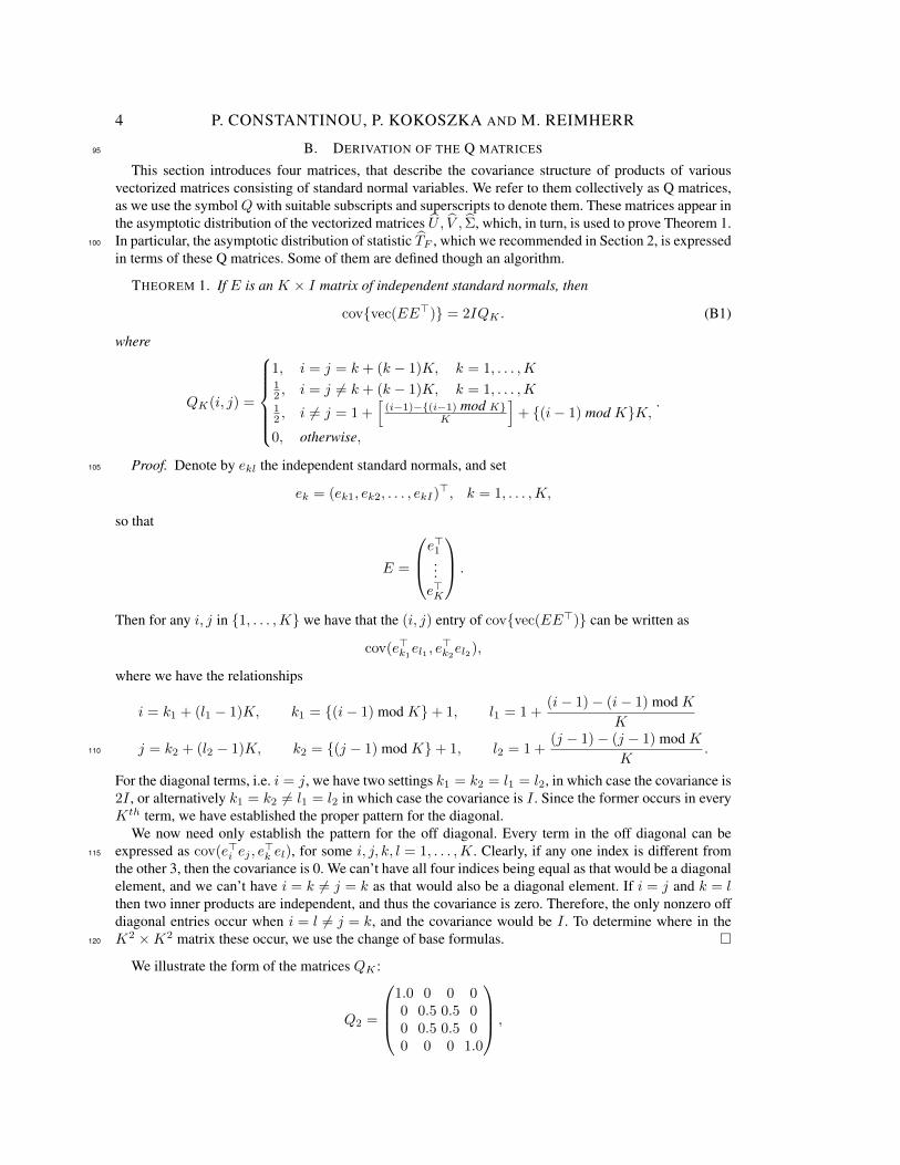
THEOREM 1. If E is an K × I matrix of independent standard normals, then
cov{vec(EE>)} = 2IQK . (B1)
where
QK(i, j) =
1, i = j = k + (k − 1)K, k = 1, . . . ,K12 , i = j 6= k + (k − 1)K, k = 1, . . . ,K12 , i 6= j = 1 +
[(i−1)−{(i−1) mod K}
K
]+ {(i− 1) mod K}K,
0, otherwise,
.
Proof. Denote by ekl the independent standard normals, and set105
ek = (ek1, ek2, . . . , ekI)>, k = 1, . . . ,K,
so that
E =
e>1...e>K
.
Then for any i, j in {1, . . . ,K} we have that the (i, j) entry of cov{vec(EE>)} can be written as
cov(e>k1el1 , e
>k2el2),
where we have the relationships
i = k1 + (l1 − 1)K, k1 = {(i− 1) mod K}+ 1, l1 = 1 +(i− 1)− (i− 1) mod K
K
j = k2 + (l2 − 1)K, k2 = {(j − 1) mod K}+ 1, l2 = 1 +(j − 1)− (j − 1) mod K
K.110
For the diagonal terms, i.e. i = j, we have two settings k1 = k2 = l1 = l2, in which case the covariance is2I , or alternatively k1 = k2 6= l1 = l2 in which case the covariance is I . Since the former occurs in everyKth term, we have established the proper pattern for the diagonal.
We now need only establish the pattern for the off diagonal. Every term in the off diagonal can beexpressed as cov(e>i ej , e
>k el), for some i, j, k, l = 1, . . . ,K. Clearly, if any one index is different from115
the other 3, then the covariance is 0. We can’t have all four indices being equal as that would be a diagonalelement, and we can’t have i = k 6= j = k as that would also be a diagonal element. If i = j and k = lthen two inner products are independent, and thus the covariance is zero. Therefore, the only nonzero offdiagonal entries occur when i = l 6= j = k, and the covariance would be I . To determine where in theK2 ×K2 matrix these occur, we use the change of base formulas. �120
We illustrate the form of the matrices QK :
Q2 =
1.0 0 0 00 0.5 0.5 00 0.5 0.5 00 0 0 1.0
,
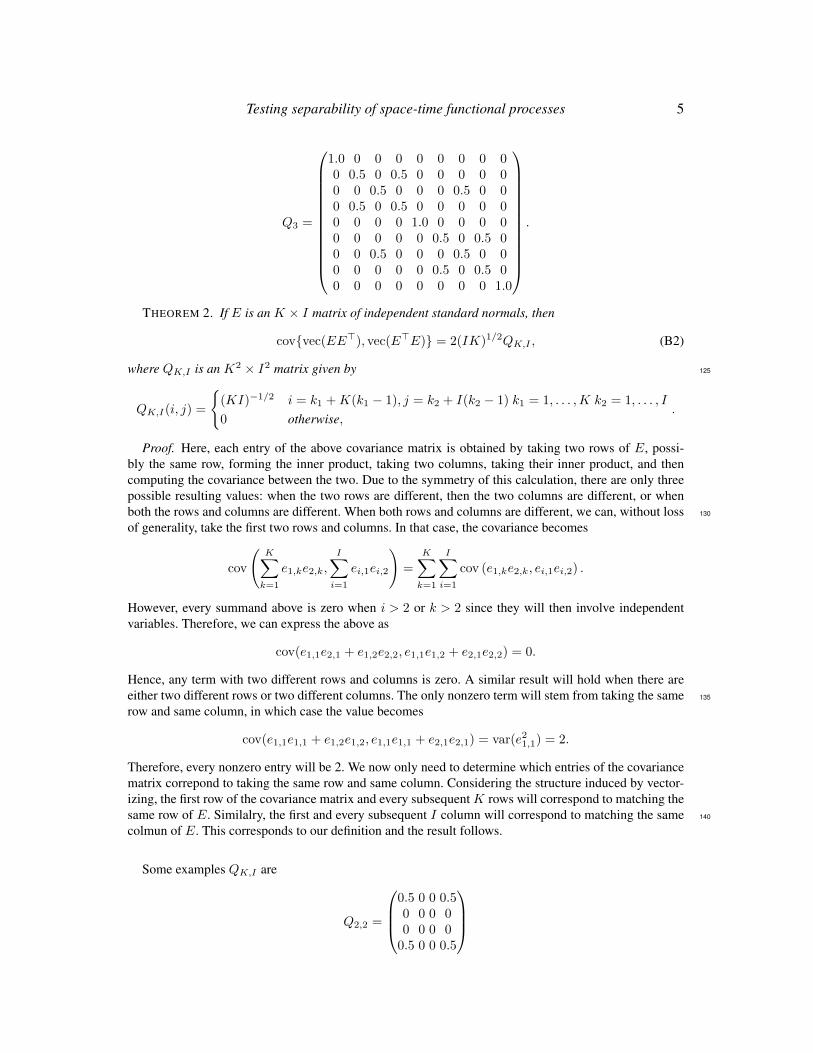
Testing separability of space-time functional processes 5
Q3 =
1.0 0 0 0 0 0 0 0 00 0.5 0 0.5 0 0 0 0 00 0 0.5 0 0 0 0.5 0 00 0.5 0 0.5 0 0 0 0 00 0 0 0 1.0 0 0 0 00 0 0 0 0 0.5 0 0.5 00 0 0.5 0 0 0 0.5 0 00 0 0 0 0 0.5 0 0.5 00 0 0 0 0 0 0 0 1.0
.
THEOREM 2. If E is an K × I matrix of independent standard normals, then
cov{vec(EE>), vec(E>E)} = 2(IK)1/2QK,I , (B2)
where QK,I is an K2 × I2 matrix given by 125
QK,I(i, j) =
{(KI)−1/2 i = k1 +K(k1 − 1), j = k2 + I(k2 − 1) k1 = 1, . . . ,K k2 = 1, . . . , I
0 otherwise,.
Proof. Here, each entry of the above covariance matrix is obtained by taking two rows of E, possi-bly the same row, forming the inner product, taking two columns, taking their inner product, and thencomputing the covariance between the two. Due to the symmetry of this calculation, there are only threepossible resulting values: when the two rows are different, then the two columns are different, or whenboth the rows and columns are different. When both rows and columns are different, we can, without loss 130
of generality, take the first two rows and columns. In that case, the covariance becomes
cov
(K∑
k=1
e1,ke2,k,
I∑i=1
ei,1ei,2
)=
K∑k=1
I∑i=1
cov (e1,ke2,k, ei,1ei,2) .
However, every summand above is zero when i > 2 or k > 2 since they will then involve independentvariables. Therefore, we can express the above as
cov(e1,1e2,1 + e1,2e2,2, e1,1e1,2 + e2,1e2,2) = 0.
Hence, any term with two different rows and columns is zero. A similar result will hold when there areeither two different rows or two different columns. The only nonzero term will stem from taking the same 135
row and same column, in which case the value becomes
cov(e1,1e1,1 + e1,2e1,2, e1,1e1,1 + e2,1e2,1) = var(e21,1) = 2.
Therefore, every nonzero entry will be 2. We now only need to determine which entries of the covariancematrix correpond to taking the same row and same column. Considering the structure induced by vector-izing, the first row of the covariance matrix and every subsequent K rows will correspond to matching thesame row of E. Similalry, the first and every subsequent I column will correspond to matching the same 140
colmun of E. This corresponds to our definition and the result follows.
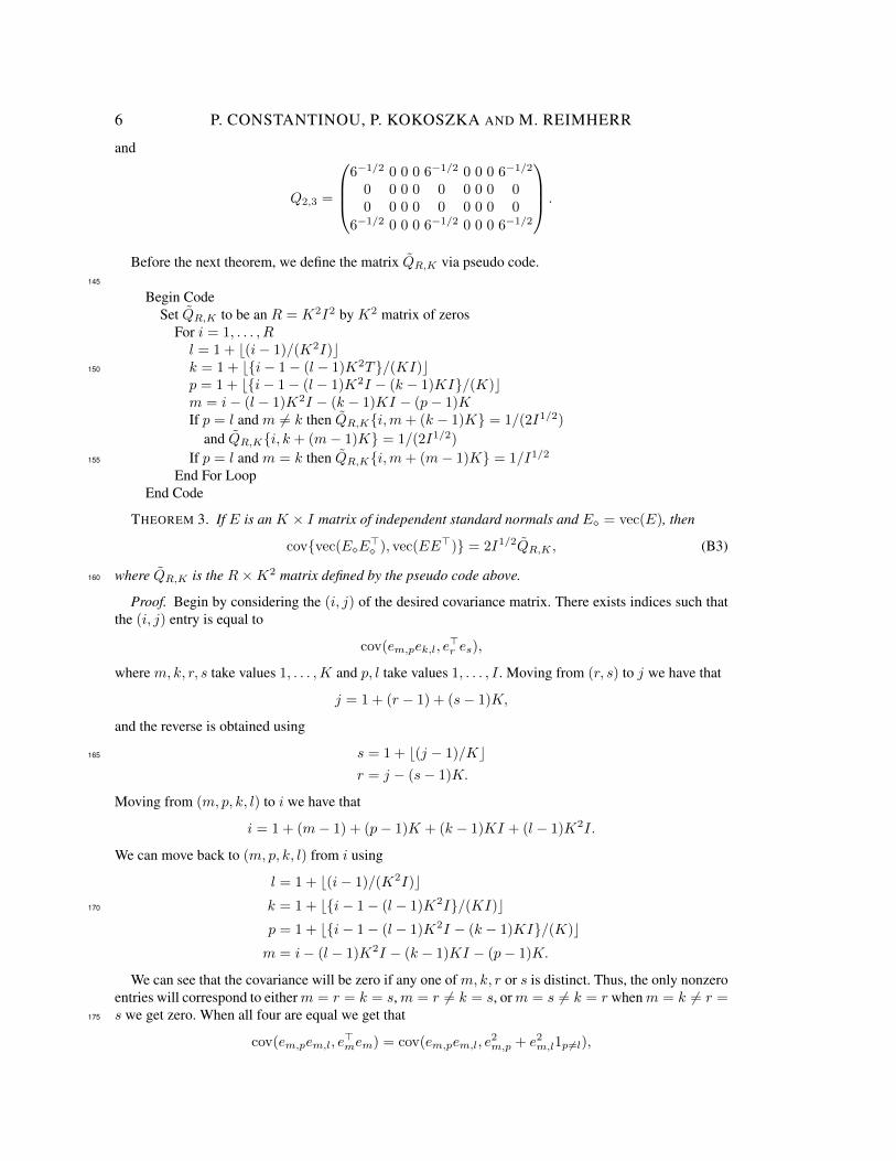
Some examples QK,I are
Q2,2 =
0.5 0 0 0.50 0 0 00 0 0 0
0.5 0 0 0.5
6 P. CONSTANTINOU, P. KOKOSZKA AND M. REIMHERR
and
Q2,3 =
6−1/2 0 0 0 6−1/2 0 0 0 6−1/2
0 0 0 0 0 0 0 0 00 0 0 0 0 0 0 0 0
6−1/2 0 0 0 6−1/2 0 0 0 6−1/2
.
Before the next theorem, we define the matrix QR,K via pseudo code.145
Begin CodeSet QR,K to be an R = K2I2 by K2 matrix of zeros
For i = 1, . . . , Rl = 1 + b(i− 1)/(K2I)ck = 1 + b{i− 1− (l − 1)K2T}/(KI)c150
p = 1 + b{i− 1− (l − 1)K2I − (k − 1)KI}/(K)cm = i− (l − 1)K2I − (k − 1)KI − (p− 1)KIf p = l and m 6= k then QR,K{i,m+ (k − 1)K} = 1/(2I1/2)
and QR,K{i, k + (m− 1)K} = 1/(2I1/2)
If p = l and m = k then QR,K{i,m+ (m− 1)K} = 1/I1/2155
End For LoopEnd Code
THEOREM 3. If E is an K × I matrix of independent standard normals and E� = vec(E), then
cov{vec(E�E>� ), vec(EE>)} = 2I1/2QR,K , (B3)
where QR,K is the R×K2 matrix defined by the pseudo code above.160
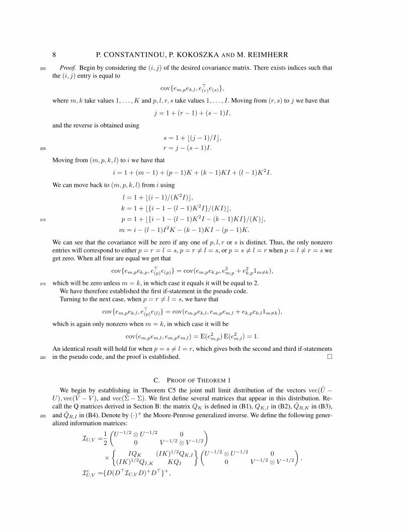
Proof. Begin by considering the (i, j) of the desired covariance matrix. There exists indices such thatthe (i, j) entry is equal to
cov(em,pek,l, e>r es),
where m, k, r, s take values 1, . . . ,K and p, l take values 1, . . . , I . Moving from (r, s) to j we have that
j = 1 + (r − 1) + (s− 1)K,
and the reverse is obtained using
s = 1 + b(j − 1)/Kc165
r = j − (s− 1)K.
Moving from (m, p, k, l) to i we have that
i = 1 + (m− 1) + (p− 1)K + (k − 1)KI + (l − 1)K2I.
We can move back to (m, p, k, l) from i using
l = 1 + b(i− 1)/(K2I)ck = 1 + b{i− 1− (l − 1)K2I}/(KI)c170
p = 1 + b{i− 1− (l − 1)K2I − (k − 1)KI}/(K)cm = i− (l − 1)K2I − (k − 1)KI − (p− 1)K.
We can see that the covariance will be zero if any one of m, k, r or s is distinct. Thus, the only nonzeroentries will correspond to eitherm = r = k = s,m = r 6= k = s, orm = s 6= k = r whenm = k 6= r =s we get zero. When all four are equal we get that175
cov(em,pem,l, e>mem) = cov(em,pem,l, e
2m,p + e2
m,l1p 6=l),
Testing separability of space-time functional processes 7
which will be zero unless p = l, in which case it equals
cov(e2m,p, e
2m,p) = {E(e4
m,p)− E(e2m,p)2} = 2.
We have therefore established the first if-statement in the pseudo code.Turning to the next case, when m = r 6= k = s, we have that
cov(em,pek,l, e>mek) = cov(em,pek,l, em,pek,p + em,lek,l1l 6=p),
which is again only nonzero when p = l, in which case it will be
cov(em,pek,p, em,pek,p) = E(e2m,p) E(e2
k,p) = 1.
An identical result will hold for whenm = s 6= k = r, which gives both the second and third if-statements 180
in the pseudo code, and the proof is established. �
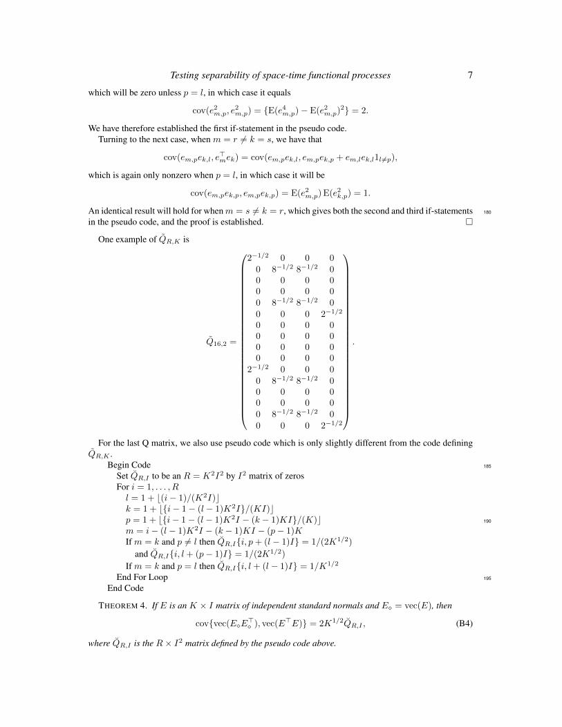
One example of QR,K is
Q16,2 =
2−1/2 0 0 00 8−1/2 8−1/2 00 0 0 00 0 0 00 8−1/2 8−1/2 00 0 0 2−1/2
0 0 0 00 0 0 00 0 0 00 0 0 0
2−1/2 0 0 00 8−1/2 8−1/2 00 0 0 00 0 0 00 8−1/2 8−1/2 00 0 0 2−1/2
.
For the last Q matrix, we also use pseudo code which is only slightly different from the code definingQR,K .
Begin Code 185
Set QR,I to be an R = K2I2 by I2 matrix of zerosFor i = 1, . . . , Rl = 1 + b(i− 1)/(K2I)ck = 1 + b{i− 1− (l − 1)K2I}/(KI)cp = 1 + b{i− 1− (l − 1)K2I − (k − 1)KI}/(K)c 190
m = i− (l − 1)K2I − (k − 1)KI − (p− 1)KIf m = k and p 6= l then QR,I{i, p+ (l − 1)I} = 1/(2K1/2)
and QR,I{i, l + (p− 1)I} = 1/(2K1/2)
If m = k and p = l then QR,I{i, l + (l − 1)I} = 1/K1/2
End For Loop 195
End Code
THEOREM 4. If E is an K × I matrix of independent standard normals and E� = vec(E), then
cov{vec(E�E>� ), vec(E>E)} = 2K1/2QR,I , (B4)
where QR,I is the R× I2 matrix defined by the pseudo code above.
8 P. CONSTANTINOU, P. KOKOSZKA AND M. REIMHERR
Proof. Begin by considering the (i, j) of the desired covariance matrix. There exists indices such that200
the (i, j) entry is equal to
cov{em,pek,l, e>(r)e(s)},
where m, k take values 1, . . . ,K and p, l, r, s take values 1, . . . , I . Moving from (r, s) to j we have that
j = 1 + (r − 1) + (s− 1)I,
and the reverse is obtained using
s = 1 + b(j − 1)/Ic,r = j − (s− 1)I.205
Moving from (m, p, k, l) to i we have that
i = 1 + (m− 1) + (p− 1)K + (k − 1)KI + (l − 1)K2I.
We can move back to (m, p, k, l) from i using
l = 1 + b(i− 1)/(K2I)c,k = 1 + b{i− 1− (l − 1)K2I}/(KI)c,p = 1 + b{i− 1− (l − 1)K2I − (k − 1)KI}/(K)c,210
m = i− (l − 1)I2K − (k − 1)KI − (p− 1)K.
We can see that the covariance will be zero if any one of p, l, r or s is distinct. Thus, the only nonzeroentries will correspond to either p = r = l = s, p = r 6= l = s, or p = s 6= l = r when p = l 6= r = s weget zero. When all four are equal we get that
cov{em,pek,p, e>(p)e(p)} = cov(em,pek,p, e
2m,p + e2
k,p1m 6=k),
which will be zero unless m = k, in which case it equals it will be equal to 2.215
We have therefore established the first if-statement in the pseudo code.Turning to the next case, when p = r 6= l = s, we have that
cov{em,pek,l, e>(p)e(l)} = cov(em,pek,l, em,pem,l + ek,pek,l1m 6=k),
which is again only nonzero when m = k, in which case it will be
cov(em,pem,l, em,pem,l) = E(e2m,p) E(e2
m,l) = 1.
An identical result will hold for when p = s 6= l = r, which gives both the second and third if-statementsin the pseudo code, and the proof is established. �220
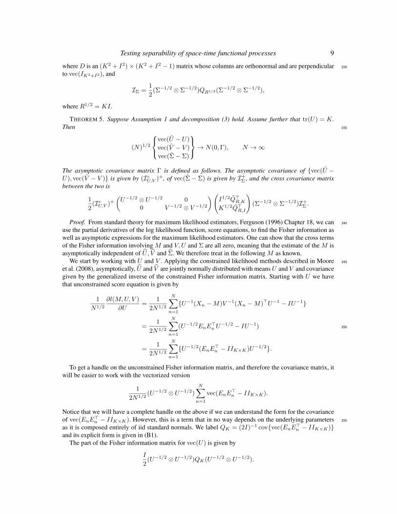
C. PROOF OF THEOREM 1We begin by establishing in Theorem C5 the joint null limit distribution of the vectors vec(U −
U), vec(V − V ), and vec(Σ− Σ). We first define several matrices that appear in this distribution. Re-call the Q matrices derived in Section B: the matrix QK is defined in (B1), QK,I in (B2), QR,K in (B3),and QR,I in (B4). Denote by (·)+ the Moore-Penrose generalized inverse. We define the following gener-225
alized information matrices:
IU,V =1
2
(U−1/2 ⊗ U−1/2 0
0 V −1/2 ⊗ V −1/2
)×{
IQK (IK)1/2QK,I
(IK)1/2QI,K KQI
}(U−1/2 ⊗ U−1/2 0
0 V −1/2 ⊗ V −1/2
),
IcU,V ={D(D>IU,VD)+D>}+,
Testing separability of space-time functional processes 9
whereD is an (K2 + I2)× (K2 + I2 − 1) matrix whose columns are orthonormal and are perpendicular 230
to vec(IK2+I2), and
IΣ =1
2(Σ−1/2 ⊗ Σ−1/2)QR1/2(Σ−1/2 ⊗ Σ−1/2),
where R1/2 = KI .
THEOREM 5. Suppose Assumption 1 and decomposition (3) hold. Assume further that tr(U) = K.Then 235
(N)1/2
vec(U − U)
vec(V − V )
vec(Σ− Σ)
→ N(0,Γ), N →∞
The asymptotic covariance matrix Γ is defined as follows. The asymptotic covariance of {vec(U −U), vec(V − V )} is given by (IcU,V )+, of vec(Σ− Σ) is given by I+
Σ , and the cross covariance matrixbetween the two is
1
2(IcU,V )+
(U−1/2 ⊗ U−1/2 0
0 V −1/2 ⊗ V −1/2
)(I1/2Q>R,K
K1/2Q>R,I
)(Σ−1/2 ⊗ Σ−1/2)I+
Σ .
Proof. From standard theory for maximum likelihood estimators, Ferguson (1996) Chapter 18, we can 240
use the partial derivatives of the log likelihood function, score equations, to find the Fisher information aswell as asymptotic expressions for the maximum likelihood estimators. One can show that the cross termsof the Fisher information involving M and V,U and Σ are all zero, meaning that the estimate of the M isasymptotically independent of U , V and Σ. We therefore treat in the following M as known.
We start by working with U and V . Applying the constrained likelihood methods described in Moore 245
et al. (2008), asymptotically, U and V are jointly normally distributed with meansU and V and covariancegiven by the generalized inverse of the constrained Fisher information matrix. Starting with U we havethat unconstrained score equation is given by
1
N1/2
∂l(M,U, V )
∂U=
1
2N1/2
N∑n=1
{U−1(Xn −M)V −1(Xn −M)>U−1 − IU−1}
=1
2N1/2
N∑n=1
(U−1/2EnE>n U−1/2 − IU−1) 250
=1
2N1/2
N∑n=1
{U−1/2(EnE>n − IIK×K)U−1/2}.
To get a handle on the unconstrained Fisher information matrix, and therefore the covariance matrix, itwill be easier to work with the vectorized version
1
2N1/2(U−1/2 ⊗ U−1/2)
N∑n=1
vec(EnE>n − IIK×K).
Notice that we will have a complete handle on the above if we can understand the form for the covarianceof vec(EnE
>n − IIK×K). However, this is a term that in no way depends on the underlying parameters 255
as it is composed entirely of iid standard normals. We label QK = (2I)−1 cov{vec(EnE>n − IIK×K)}
and its explicit form is given in (B1).The part of the Fisher information matrix for vec(U) is given by
I
2(U−1/2 ⊗ U−1/2)QK(U−1/2 ⊗ U−1/2).
10 P. CONSTANTINOU, P. KOKOSZKA AND M. REIMHERR
Identical arguments give that the part of the Fisher information matrix for vec(V ) is given by
K
2(V −1/2 ⊗ V −1/2)QI(V −1/2 ⊗ V −1/2).
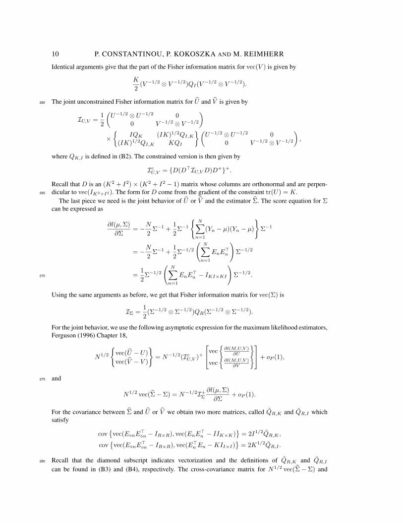
The joint unconstrained Fisher information matrix for U and V is given by260
IU,V =1
2
(U−1/2 ⊗ U−1/2 0
0 V −1/2 ⊗ V −1/2
)×{
IQK (IK)1/2QI,K
(IK)1/2QI,K KQI
}(U−1/2 ⊗ U−1/2 0
0 V −1/2 ⊗ V −1/2
),
where QK,I is defined in (B2). The constrained version is then given by
IcU,V = {D(D>IU,VD)D+}+.
Recall that D is an (K2 + I2)× (K2 + I2 − 1) matrix whose columns are orthonormal and are perpen-dicular to vec(IK2+I2). The form for D come from the gradient of the constraint tr(U) = K.265
The last piece we need is the joint behavior of U or V and the estimator Σ. The score equation for Σcan be expressed as
∂l(µ,Σ)
∂Σ= −N
2Σ−1 +
1
2Σ−1
{N∑
n=1
(Yn − µ)(Yn − µ)
}Σ−1
= −N2
Σ−1 +1
2Σ−1/2
(N∑
n=1
EnE>n
)Σ−1/2
=1
2Σ−1/2
(N∑
n=1
EnE>n − IKI×KI
)Σ−1/2.270
Using the same arguments as before, we get that Fisher information matrix for vec(Σ) is
IΣ =1
2(Σ−1/2 ⊗ Σ−1/2)QR(Σ−1/2 ⊗ Σ−1/2).
For the joint behavior, we use the following asymptotic expression for the maximum likelihood estimators,Ferguson (1996) Chapter 18,
N1/2
{vec(U − U)
vec(V − V )
}= N−1/2(IcU,V )+
vec{
∂l(M,U,V )∂U
}vec{
∂l(M,U,V )∂V
}+ oP (1),
and275
N1/2 vec(Σ− Σ) = N−1/2I+Σ
∂l(µ,Σ)
∂Σ+ oP (1).
For the covariance between Σ and U or V we obtain two more matrices, called QR,K and QR,I whichsatisfy
cov{
vec(E�nE>�n − IR×R), vec(EnE
>n − IIK×K)
}= 2I1/2QR,K ,
cov{
vec(E�nE>�n − IR×R), vec(E>n En −KII×I)
}= 2K1/2QR,I .
Recall that the diamond subscript indicates vectorization and the definitions of QR,K and QR,I280
can be found in (B3) and (B4), respectively. The cross-covariance matrix for N1/2 vec(Σ− Σ) and
Testing separability of space-time functional processes 11
N1/2 vec(U − U) is then given by
(IcU,V )+ cov
vec(N−1/2 ∂l(M,U,V )
∂U
)vec(N−1/2 ∂l(M,U,V )
∂V
) , vec
{N−1/2 ∂l(M,Σ)
∂Σ
} I+Σ
=1
2(IcU,V )+
(U−1/2 ⊗ U−1/2 0
0 V −1/2 ⊗ V −1/2
)(I1/2Q>R,K
K1/2Q>R,I
)(Σ−1/2 ⊗ Σ−1/2)I+
Σ
285
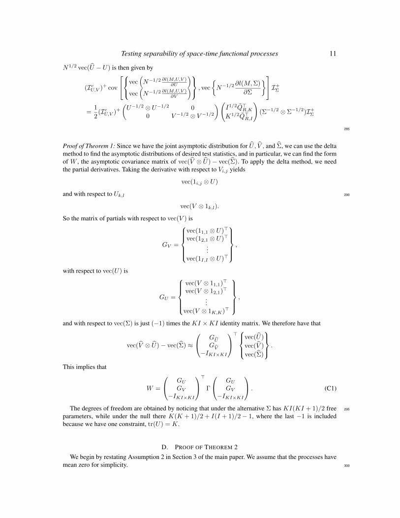
Proof of Theorem 1: Since we have the joint asymptotic distribution for U , V , and Σ, we can use the deltamethod to find the asymptotic distributions of desired test statistics, and in particular, we can find the formof W , the asymptotic covariance matrix of vec(V ⊗ U)− vec(Σ). To apply the delta method, we needthe partial derivatives. Taking the derivative with respect to Vi,j yields
vec(1i,j ⊗ U)
and with respect to Uk,l 290
vec(V ⊗ 1k,l).
So the matrix of partials with respect to vec(V ) is
GV =
vec(11,1 ⊗ U)>
vec(12,1 ⊗ U)>
...vec(1I,I ⊗ U)>
,
with respect to vec(U) is
GU =
vec(V ⊗ 11,1)>
vec(V ⊗ 12,1)>
...vec(V ⊗ 1K,K)>
,
and with respect to vec(Σ) is just (−1) times the KI ×KI identity matrix. We therefore have that
vec(V ⊗ U)− vec(Σ) ≈
GUGV
−IKI×KI
>
vec(U)
vec(V )
vec(Σ)
.
This implies that
W =
GU
GV
−IKI×KI
> Γ
GU
GV
−IKI×KI
. (C1)
The degrees of freedom are obtained by noticing that under the alternative Σ has KI(KI + 1)/2 free 295
parameters, while under the null there K(K + 1)/2 + I(I + 1)/2− 1, where the last −1 is includedbecause we have one constraint, tr(U) = K.
D. PROOF OF THEOREM 2We begin by restating Assumption 2 in Section 3 of the main paper. We assume that the processes have
mean zero for simplicity. 300
12 P. CONSTANTINOU, P. KOKOSZKA AND M. REIMHERR
Assumption 1. Assume that the Xn are independent and identically distributed mean zero Gaussianprocesses in L2(S × T ) with separable covariance σ(s, s′, t, t′) = U(s, s′)V(t, t′). Assume the functionsare scaled such that tr(U) =
∑U(sk, sk) =
∑U(k, k) = K.
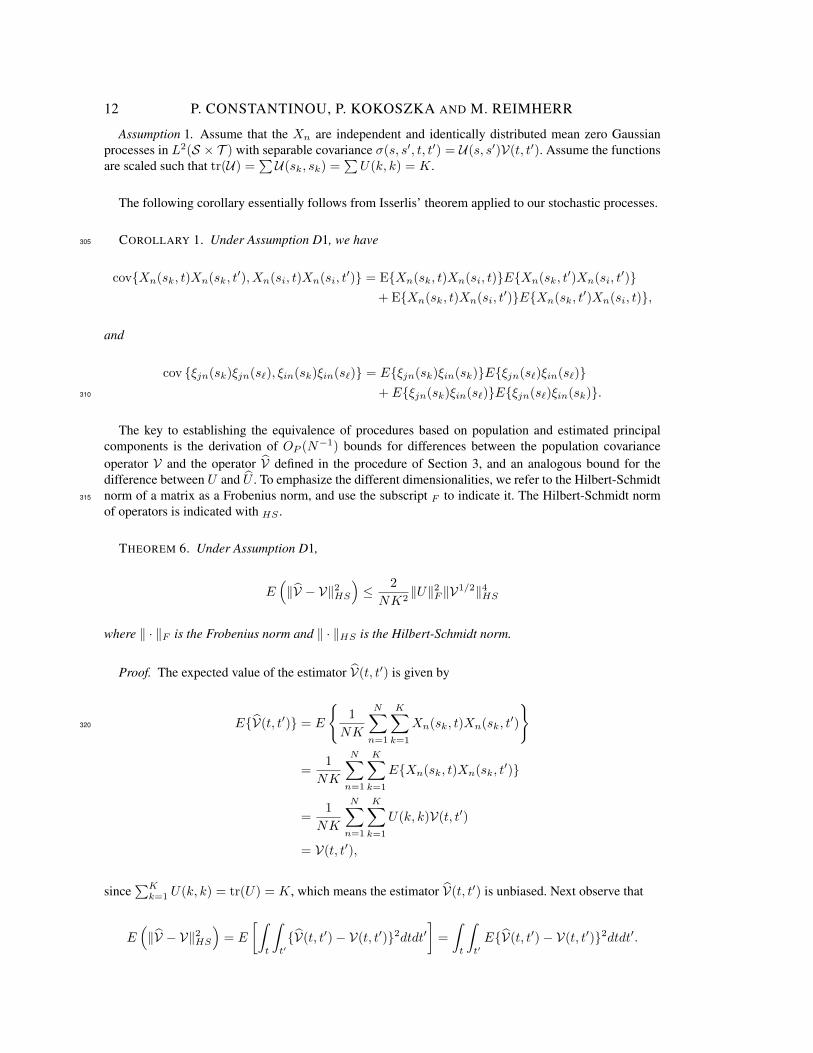
The following corollary essentially follows from Isserlis’ theorem applied to our stochastic processes.
COROLLARY 1. Under Assumption D1, we have305
cov{Xn(sk, t)Xn(sk, t′), Xn(si, t)Xn(si, t
′)} = E{Xn(sk, t)Xn(si, t)}E{Xn(sk, t′)Xn(si, t
′)}+ E{Xn(sk, t)Xn(si, t
′)}E{Xn(sk, t′)Xn(si, t)},
and
cov {ξjn(sk)ξjn(s`), ξin(sk)ξin(s`)} = E{ξjn(sk)ξin(sk)}E{ξjn(s`)ξin(s`)}+ E{ξjn(sk)ξin(s`)}E{ξjn(s`)ξin(sk)}.310
The key to establishing the equivalence of procedures based on population and estimated principalcomponents is the derivation of OP (N−1) bounds for differences between the population covarianceoperator V and the operator V defined in the procedure of Section 3, and an analogous bound for thedifference between U and U . To emphasize the different dimensionalities, we refer to the Hilbert-Schmidtnorm of a matrix as a Frobenius norm, and use the subscript F to indicate it. The Hilbert-Schmidt norm315
of operators is indicated with HS .
THEOREM 6. Under Assumption D1,
E(‖V − V‖2HS
)≤ 2
NK2‖U‖2F ‖V1/2‖4HS
where ‖ · ‖F is the Frobenius norm and ‖ · ‖HS is the Hilbert-Schmidt norm.
Proof. The expected value of the estimator V(t, t′) is given by
E{V(t, t′)} = E
{1
NK
N∑n=1
K∑k=1
Xn(sk, t)Xn(sk, t′)
}320
=1
NK
N∑n=1
K∑k=1
E{Xn(sk, t)Xn(sk, t′)}
=1
NK
N∑n=1
K∑k=1
U(k, k)V(t, t′)
= V(t, t′),
since∑K
k=1 U(k, k) = tr(U) = K, which means the estimator V(t, t′) is unbiased. Next observe that
E(‖V − V‖2HS
)= E
[∫t
∫t′{V(t, t′)− V(t, t′)}2dtdt′
]=
∫t
∫t′E{V(t, t′)− V(t, t′)}2dtdt′.
Testing separability of space-time functional processes 13
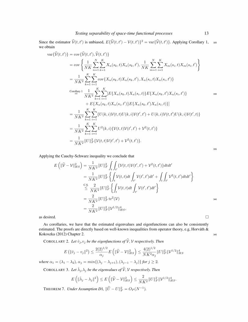
Since the estimator V(t, t′) is unbiased, E{V(t, t′)− V(t, t′)}2 = var{V(t, t′)}. Applying Corollary 1, 325
we obtain
var{V(t, t′)} = cov{V(t, t′), V(t, t′)}
= cov
{1
NK
N∑n=1
K∑k=1
Xn(sk, t)Xn(sk, t′),
1
NK
N∑m=1
K∑i=1
Xm(si, t)Xm(si, t′)
}
=1
NK2
K∑k=1
K∑i=1
cov{Xn(sk, t)Xn(sk, t′), Xn(si, t)Xn(si, t
′)}
Corollary 1=
1
NK2
K∑k=1
K∑i=1
[E{Xn(sk, t)Xn(si, t)}E{Xn(sk, t′)Xn(si, t
′)} 330
+ E{Xn(sk, t)Xn(si, t′)}E{Xn(sk, t
′)Xn(si, t)}]
=1
NK2
K∑k=1
K∑i=1
{U(k, i)V(t, t)U(k, i)V(t′, t′) + U(k, i)V(t, t′)U(k, i)V(t′, t)}
=1
NK2
K∑k=1
K∑i=1
U2(k, i){V(t, t)V(t′, t′) + V2(t, t′)}
=1
NK2‖U‖2F {V(t, t)V(t′, t′) + V2(t, t′)}.
335
Applying the Cauchy-Schwarz inequality we conclude that
E(‖V − V‖2HS
)=
1
NK2‖U‖2F
∫t
∫t′{V(t, t)V(t′, t′) + V2(t, t′)}dtdt′
=1
NK2‖U‖2F
{∫t
V(t, t)dt
∫t′V(t′, t′)dt′ +
∫t
∫t′V2(t, t′)dtdt′
}C.S.≤ 2
NK2‖U‖2F
{∫t
V(t, t)dt
∫t′V(t′, t′)dt′
}=
2
NK2‖U‖2F tr2(V) 340
=2
NK2‖U‖2F ‖V1/2‖4HS ,
as desired. �
As corollaries, we have that the estimated eigenvalues and eigenfunctions can also be consistentlyestimated. The proofs are directly based on well-known inequalities from operator theory, e.g, Horvath &Kokoszka (2012) Chapter 2. 345
COROLLARY 2. Let vj ,vj be the eigenfunctions of V,V respectively. Then
E(‖vj − vj‖2
)≤ 2(2)1/2
αjE(‖V − V‖2HS
)≤ 4(2)1/2
NK2αj‖U‖2F ‖V1/2‖4HS
where α1 = (λ1 − λ2), αj = min{(λj − λj+1), (λj−1 − λj)} for j ≥ 2.
COROLLARY 3. Let λj ,λj be the eigenvalues of V,V respectively. Then
E(‖λj − λj‖2
)≤ E
(‖V − V‖2HS
)≤ 2
NK2‖U‖2F ‖V1/2‖4HS .
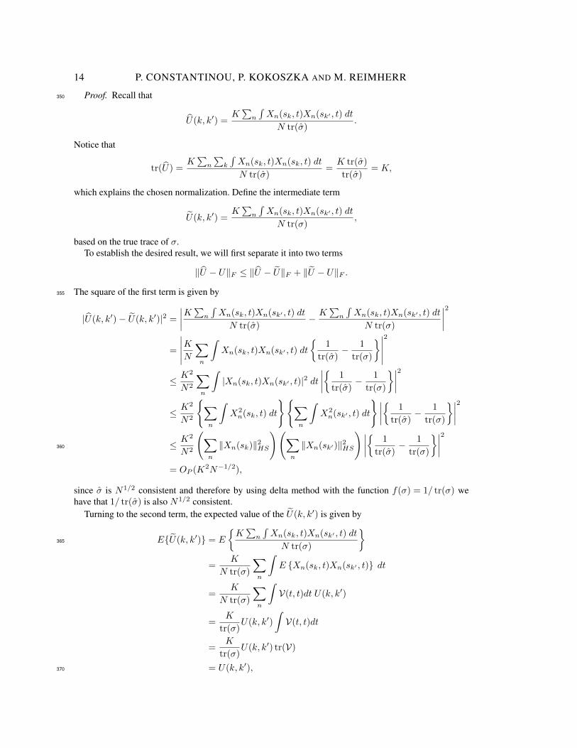
THEOREM 7. Under Assumption D1, ‖U − U‖2F = OP (N−1).
14 P. CONSTANTINOU, P. KOKOSZKA AND M. REIMHERR
Proof. Recall that350
U(k, k′) =K∑
n
∫Xn(sk, t)Xn(sk′ , t) dt
N tr(σ).
Notice that
tr(U) =K∑
n
∑k
∫Xn(sk, t)Xn(sk, t) dt
N tr(σ)=K tr(σ)
tr(σ)= K,
which explains the chosen normalization. Define the intermediate term
U(k, k′) =K∑
n
∫Xn(sk, t)Xn(sk′ , t) dt
N tr(σ),
based on the true trace of σ.To establish the desired result, we will first separate it into two terms
‖U − U‖F ≤ ‖U − U‖F + ‖U − U‖F .
The square of the first term is given by355
|U(k, k′)− U(k, k′)|2 =
∣∣∣∣K∑n
∫Xn(sk, t)Xn(sk′ , t) dt
N tr(σ)−K∑
n
∫Xn(sk, t)Xn(sk′ , t) dt
N tr(σ)
∣∣∣∣2=
∣∣∣∣∣KN ∑n
∫Xn(sk, t)Xn(sk′ , t) dt
{1
tr(σ)− 1
tr(σ)
}∣∣∣∣∣2
≤ K2
N2
∑n
∫|Xn(sk, t)Xn(sk′ , t)|2 dt
∣∣∣∣{ 1
tr(σ)− 1
tr(σ)
}∣∣∣∣2≤ K2
N2
{∑n
∫X2
n(sk, t) dt
}{∑n
∫X2
n(sk′ , t) dt
}∣∣∣∣{ 1
tr(σ)− 1
tr(σ)
}∣∣∣∣2≤ K2
N2
(∑n
‖Xn(sk)‖2HS
)(∑n
‖Xn(sk′)‖2HS
)∣∣∣∣{ 1
tr(σ)− 1
tr(σ)
}∣∣∣∣2360
= OP (K2N−1/2),
since σ is N1/2 consistent and therefore by using delta method with the function f(σ) = 1/ tr(σ) wehave that 1/ tr(σ) is also N1/2 consistent.
Turning to the second term, the expected value of the U(k, k′) is given by
E{U(k, k′)} = E
{K∑
n
∫Xn(sk, t)Xn(sk′ , t) dt
N tr(σ)
}365
=K
N tr(σ)
∑n
∫E {Xn(sk, t)Xn(sk′ , t)} dt
=K
N tr(σ)
∑n
∫V(t, t)dt U(k, k′)
=K
tr(σ)U(k, k′)
∫V(t, t)dt
=K
tr(σ)U(k, k′) tr(V)
= U(k, k′),370
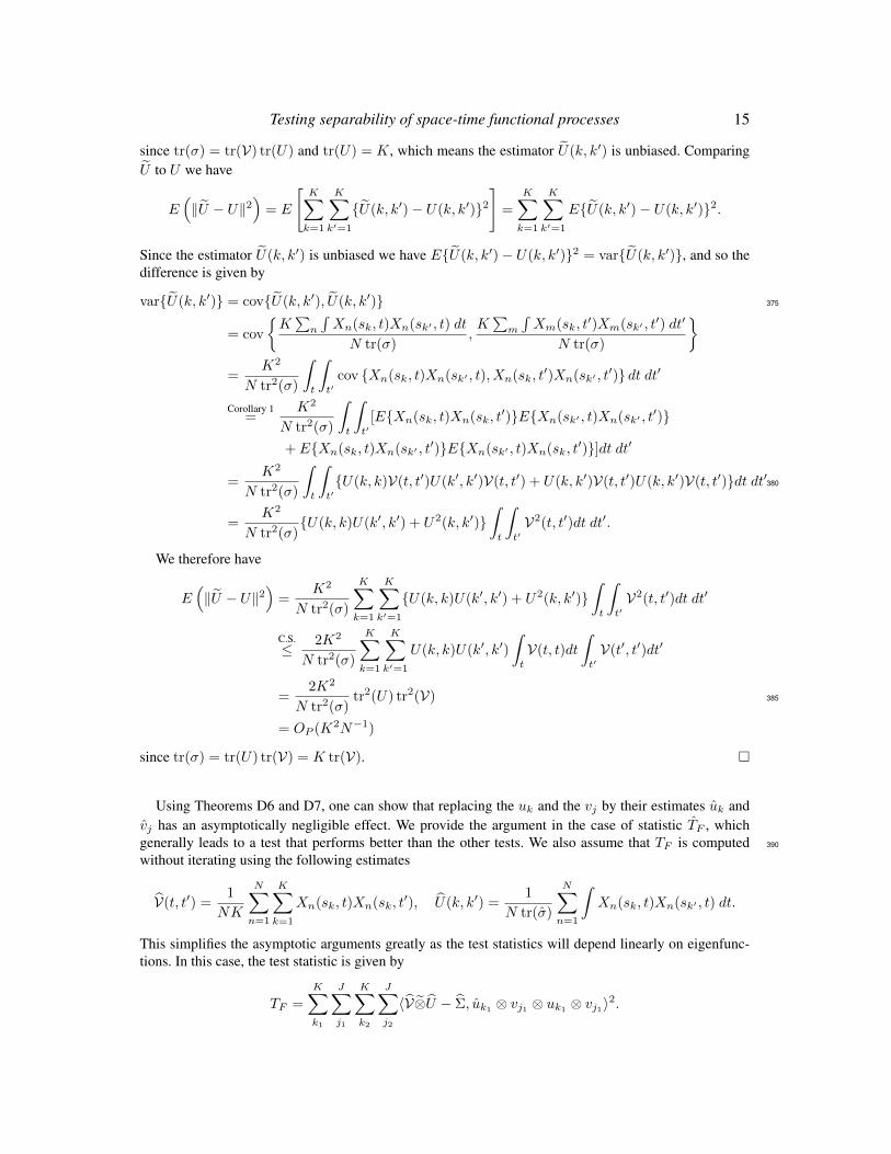
Testing separability of space-time functional processes 15
since tr(σ) = tr(V) tr(U) and tr(U) = K, which means the estimator U(k, k′) is unbiased. ComparingU to U we have
E(‖U − U‖2
)= E
[K∑
k=1
K∑k′=1
{U(k, k′)− U(k, k′)}2]
=
K∑k=1
K∑k′=1
E{U(k, k′)− U(k, k′)}2.
Since the estimator U(k, k′) is unbiased we have E{U(k, k′)− U(k, k′)}2 = var{U(k, k′)}, and so thedifference is given by
var{U(k, k′)} = cov{U(k, k′), U(k, k′)} 375
= cov
{K∑
n
∫Xn(sk, t)Xn(sk′ , t) dt
N tr(σ),K∑
m
∫Xm(sk, t
′)Xm(sk′ , t′) dt′
N tr(σ)
}=
K2
N tr2(σ)
∫t
∫t′
cov {Xn(sk, t)Xn(sk′ , t), Xn(sk, t′)Xn(sk′ , t′)} dt dt′
Corollary 1=
K2
N tr2(σ)
∫t
∫t′
[E{Xn(sk, t)Xn(sk, t′)}E{Xn(sk′ , t)Xn(sk′ , t′)}
+ E{Xn(sk, t)Xn(sk′ , t′)}E{Xn(sk′ , t)Xn(sk, t′)}]dt dt′
=K2
N tr2(σ)
∫t
∫t′{U(k, k)V(t, t′)U(k′, k′)V(t, t′) + U(k, k′)V(t, t′)U(k, k′)V(t, t′)}dt dt′380
=K2
N tr2(σ){U(k, k)U(k′, k′) + U2(k, k′)}
∫t
∫t′V2(t, t′)dt dt′.
We therefore have
E(‖U − U‖2
)=
K2
N tr2(σ)
K∑k=1
K∑k′=1
{U(k, k)U(k′, k′) + U2(k, k′)}∫t
∫t′V2(t, t′)dt dt′
C.S.≤ 2K2
N tr2(σ)
K∑k=1
K∑k′=1
U(k, k)U(k′, k′)
∫t
V(t, t)dt
∫t′V(t′, t′)dt′
=2K2
N tr2(σ)tr2(U) tr2(V) 385
= OP (K2N−1)
since tr(σ) = tr(U) tr(V) = K tr(V). �
Using Theorems D6 and D7, one can show that replacing the uk and the vj by their estimates uk andvj has an asymptotically negligible effect. We provide the argument in the case of statistic TF , whichgenerally leads to a test that performs better than the other tests. We also assume that TF is computed 390
without iterating using the following estimates
V(t, t′) =1
NK
N∑n=1
K∑k=1
Xn(sk, t)Xn(sk, t′), U(k, k′) =
1
N tr(σ)
N∑n=1
∫Xn(sk, t)Xn(sk′ , t) dt.
This simplifies the asymptotic arguments greatly as the test statistics will depend linearly on eigenfunc-tions. In this case, the test statistic is given by
TF =
K∑k1
J∑j1
K∑k2
J∑j2
〈V⊗U − Σ, uk1⊗ vj1 ⊗ uk1
⊗ vj1〉2.
16 P. CONSTANTINOU, P. KOKOSZKA AND M. REIMHERR
THEOREM 8. Denote by TF the statistic computed using the estimators uk and vj and by T †F therandom variable computed using the population functions uk and vj . If Assumption D1 holds, then395
TF − T †F = OP (N−1/2).
Proof. To lighten the notation, we drop the superscript F . First notice that
T =
K∑k1
J∑j1
K∑k2
J∑j2
N〈V ⊗ U − Σ, uk1⊗ vj1 ⊗ uk2
⊗ vj2〉2,
with an analogous formula for T †. Let T ∗ = V ⊗ U − Σ. By using the triangle inequality we have that∣∣∣∣∣∣K∑k1
J∑j1
K∑k2
J∑j2
N〈T ∗, uk1 ⊗ vj1 ⊗ uk2 ⊗ vj2〉2 −K∑k1
J∑j1
K∑k2
J∑j2
N〈T ∗, uk1 ⊗ vj1 ⊗ uk2 ⊗ vj2〉2∣∣∣∣∣∣
≤ NK∑k1
J∑j1
K∑k2
J∑j2
∣∣〈T ∗, uk1⊗ vj1 ⊗ uk2
⊗ vj2〉2 − 〈T ∗, uk1⊗ vj1 ⊗ uk2
⊗ vj2〉2∣∣ .400
By using the formula a2 − b2 = (a− b)(a+ b) and the linearity of the inner product we obtain∣∣〈T ∗, uk1⊗ vj1 ⊗ uk2
⊗ vj2〉2 − 〈T ∗, uk1⊗ vj1 ⊗ uk2
⊗ vj2〉2∣∣ = |〈T ∗, uk1
⊗ vj1 ⊗ uk2⊗ vj2 − uk1
⊗ vj1 ⊗ uk2⊗ vj2〉|
× |〈T ∗, uk1⊗ vj1 ⊗ uk2
⊗ vj2 + uk1⊗ vj1 ⊗ uk2
⊗ vj2〉| .
Applying the Cauchy-Schwarz inequality, the above is bounded by
‖T ∗‖2‖uk1⊗ vj1 ⊗ uk2
⊗ vj2 − uk1⊗ vj1 ⊗ uk2
⊗ vj2‖‖uk1⊗ vj1 ⊗ uk2
⊗ vj2 + uk1⊗ vj1 ⊗ uk2
⊗ vj2‖405
≤ 2‖T ∗‖2‖uk1 ⊗ vj1 ⊗ uk2 ⊗ vj2 − uk1 ⊗ vj1 ⊗ uk2 ⊗ vj2‖.
We have that
‖uk1⊗ vj1 ⊗ uk2
⊗ vj2 − uk1⊗ vj1 ⊗ uk2
⊗ vj2‖= ‖uk1
⊗ vj1 ⊗ uk2⊗ vj2 − uk1
⊗ vj1 ⊗ uk2⊗ vj2 + uk1
⊗ vj1 ⊗ uk2⊗ vj2 − uk1
⊗ vj1 ⊗ uk2⊗ vj2‖
≤ ‖uk1⊗ vj1 ⊗ uk2
⊗ vj2 − uk1⊗ vj1 ⊗ uk2
⊗ vj2‖+ ‖uk1⊗ vj1 ⊗ uk2
⊗ vj2 − uk1⊗ vj1 ⊗ uk2
⊗ vj2‖410
= ‖uk1− uk1
‖+ ‖uk1⊗ vj1 ⊗ uk2
⊗ vj2 − uk1⊗ vj1 ⊗ uk2
⊗ vj2‖= ‖uk1
− uk1‖+ ‖uk1
⊗ vj1 ⊗ uk2⊗ vj2 ± uk1
⊗ vj1 ⊗ uk2⊗ vj2 − uk1
⊗ vj1 ⊗ uk2⊗ vj2‖
≤ ‖uk1− uk1
‖+ ‖uk1⊗ vj1 ⊗ uk2
⊗ vj2 − uk1⊗ vj1 ⊗ uk2
⊗ vj2‖+ ‖uk1⊗ vj1 ⊗ uk2
⊗ vj2 − uk1⊗ vj1 ⊗ uk2
⊗ vj2‖= ‖uk1
− uk1‖+ ‖vj1 − vj1‖+ ‖uk1
⊗ vj1 ⊗ uk2⊗ vj2 − uk1
⊗ vj1 ⊗ uk2⊗ vj2‖
= ‖uk1− uk1
‖+ ‖vj1 − vj1‖+ ‖uk1⊗ vj1 ⊗ uk2
⊗ vj2 ± uk1⊗ vj1 ⊗ uk2
⊗ vj2 − uk1⊗ vj1 ⊗ uk2
⊗ vj2‖415
≤ ‖uk1− uk1
‖+ ‖vj1 − vj1‖+ ‖uk1⊗ vj1 ⊗ uk2
⊗ vj2 − uk1⊗ vj1 ⊗ uk2
⊗ vj2‖+ ‖uk1
⊗ vj1 ⊗ uk2⊗ vj2 − uk1
⊗ vj1 ⊗ uk2⊗ vj2‖
= ‖uk1− uk1
‖+ ‖vj1 − vj1‖+ ‖uk2− uk2
‖+ ‖vj2 − vj2‖
≤ 2(2)1/2
βk1
‖U − U‖+2(2)1/2
αj1
‖V − V ‖+2(2)1/2
βk2
‖U − U‖+2(2)1/2
αj2
‖V − V ‖,
where α1 = (λ1 − λ2), αj1 = min{(λj1 − λj1+1), (λj1−1 − λj1)} for j1 ≥ 2, β1 = (µ1 − µ2) and420
βk1 = min{(µk1 − µk1+1), (µk1−1 − µk1)} for k1 ≥ 2. Here λ1, . . . , λJ are the eigenvalues of V andµ1, . . . , µK are the eigenvalues of U .
Testing separability of space-time functional processes 17
To sum up we have∣∣∣∣∣∣K∑k1
J∑j1
K∑k2
J∑j2
N〈T ∗, uk1⊗ vj1 ⊗ uk2
⊗ vj2〉2 −K∑k1
J∑j1
K∑k2
J∑j2
N〈T ∗, uk1⊗ vj1 ⊗ uk2
⊗ vj2〉2∣∣∣∣∣∣
≤ NK∑k1
J∑j1
K∑k2
J∑j2
2‖T ∗‖2(
2(2)1/2
βk1
‖U − U‖+2(2)1/2
αj1
‖V − V ‖+2(2)1/2
βk2
‖U − U‖+2(2)1/2
αj2
‖V − V ‖)
425
= ‖(N)1/2T ∗‖28(2)1/2JK
J K∑k1
1
βk1
‖U − U‖+K
J∑j1
1
αj1
‖V − V ‖
= OP (N−1/2),
and the claim holds. �
E. ADDITIONAL EMPIRICAL REJECTION RATES, MORE DISCUSSION IN IRISH WIND DATA ANDAPPLICATION TO POLLUTION DATA 430
E·1. Additional simulationsWe now study the effect of increasing the number of spatial locations and the number of spatial and
temporal principal components. We will use the first spatiotemporal covariance function introduced byGneiting (2002). We use I = 100 time points equally spaced on [0, 1] and K = 16, 25 equally spacedpoints in [0, 1]× [0, 1]. We display the results, based on 1000 replications, for two extreme values of the 435
space-time interaction parameter, β = 0 and β = 1. Table 1 shows that increasing the number of spatialpoints and the number of principal components does not change our previous conclusions, i.e., only thetests TL−MC and TF are robust to the number of the principal components used with the TF having morepower.
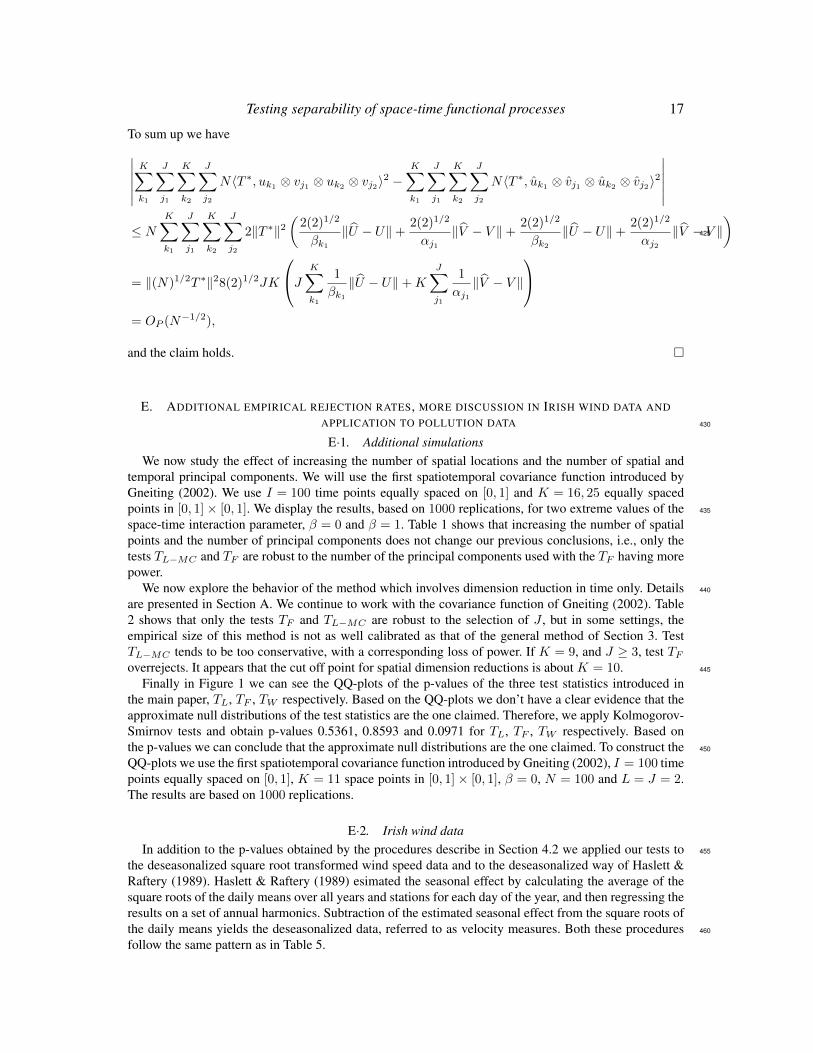
We now explore the behavior of the method which involves dimension reduction in time only. Details 440
are presented in Section A. We continue to work with the covariance function of Gneiting (2002). Table2 shows that only the tests TF and TL−MC are robust to the selection of J , but in some settings, theempirical size of this method is not as well calibrated as that of the general method of Section 3. TestTL−MC tends to be too conservative, with a corresponding loss of power. If K = 9, and J ≥ 3, test TFoverrejects. It appears that the cut off point for spatial dimension reductions is about K = 10. 445
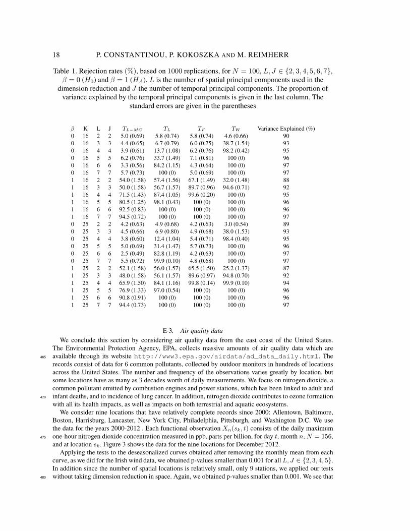
Finally in Figure 1 we can see the QQ-plots of the p-values of the three test statistics introduced inthe main paper, TL, TF , TW respectively. Based on the QQ-plots we don’t have a clear evidence that theapproximate null distributions of the test statistics are the one claimed. Therefore, we apply Kolmogorov-Smirnov tests and obtain p-values 0.5361, 0.8593 and 0.0971 for TL, TF , TW respectively. Based onthe p-values we can conclude that the approximate null distributions are the one claimed. To construct the 450
QQ-plots we use the first spatiotemporal covariance function introduced by Gneiting (2002), I = 100 timepoints equally spaced on [0, 1], K = 11 space points in [0, 1]× [0, 1], β = 0, N = 100 and L = J = 2.The results are based on 1000 replications.
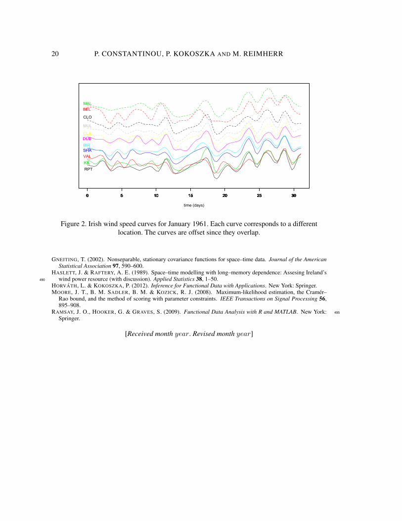
E·2. Irish wind dataIn addition to the p-values obtained by the procedures describe in Section 4.2 we applied our tests to 455
the deseasonalized square root transformed wind speed data and to the deseasonalized way of Haslett &Raftery (1989). Haslett & Raftery (1989) esimated the seasonal effect by calculating the average of thesquare roots of the daily means over all years and stations for each day of the year, and then regressing theresults on a set of annual harmonics. Subtraction of the estimated seasonal effect from the square roots ofthe daily means yields the deseasonalized data, referred to as velocity measures. Both these procedures 460
follow the same pattern as in Table 5.
18 P. CONSTANTINOU, P. KOKOSZKA AND M. REIMHERR
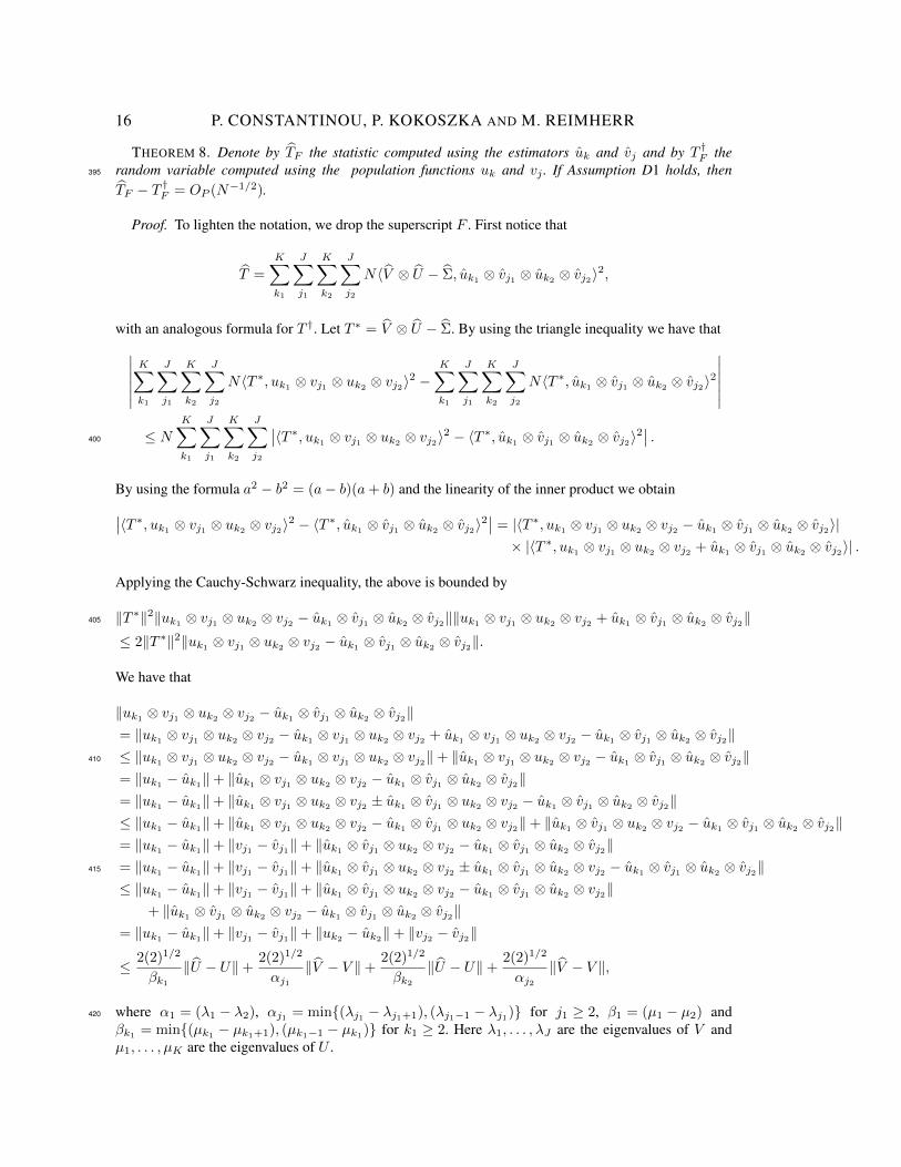
Table 1. Rejection rates (%), based on 1000 replications, for N = 100, L, J ∈ {2, 3, 4, 5, 6, 7},β = 0 (H0) and β = 1 (HA). L is the number of spatial principal components used in the
dimension reduction and J the number of temporal principal components. The proportion ofvariance explained by the temporal principal components is given in the last column. The
standard errors are given in the parentheses
β K L J TL−MC TL TF TW Variance Explained (%)0 16 2 2 5.0 (0.69) 5.8 (0.74) 5.8 (0.74) 4.6 (0.66) 900 16 3 3 4.4 (0.65) 6.7 (0.79) 6.0 (0.75) 38.7 (1.54) 930 16 4 4 3.9 (0.61) 13.7 (1.08) 6.2 (0.76) 98.2 (0.42) 950 16 5 5 6.2 (0.76) 33.7 (1.49) 7.1 (0.81) 100 (0) 960 16 6 6 3.3 (0.56) 84.2 (1.15) 4.3 (0.64) 100 (0) 970 16 7 7 5.7 (0.73) 100 (0) 5.0 (0.69) 100 (0) 971 16 2 2 54.0 (1.58) 57.4 (1.56) 67.1 (1.49) 32.0 (1.48) 881 16 3 3 50.0 (1.58) 56.7 (1.57) 89.7 (0.96) 94.6 (0.71) 921 16 4 4 71.5 (1.43) 87.4 (1.05) 99.6 (0.20) 100 (0) 951 16 5 5 80.5 (1.25) 98.1 (0.43) 100 (0) 100 (0) 961 16 6 6 92.5 (0.83) 100 (0) 100 (0) 100 (0) 961 16 7 7 94.5 (0.72) 100 (0) 100 (0) 100 (0) 970 25 2 2 4.2 (0.63) 4.9 (0.68) 4.2 (0.63) 3.0 (0.54) 890 25 3 3 4.5 (0.66) 6.9 (0.80) 4.9 (0.68) 38.0 (1.53) 930 25 4 4 3.8 (0.60) 12.4 (1.04) 5.4 (0.71) 98.4 (0.40) 950 25 5 5 5.0 (0.69) 31.4 (1.47) 5.7 (0.73) 100 (0) 960 25 6 6 2.5 (0.49) 82.8 (1.19) 4.2 (0.63) 100 (0) 970 25 7 7 5.5 (0.72) 99.9 (0.10) 4.8 (0.68) 100 (0) 971 25 2 2 52.1 (1.58) 56.0 (1.57) 65.5 (1.50) 25.2 (1.37) 871 25 3 3 48.0 (1.58) 56.1 (1.57) 89.6 (0.97) 94.8 (0.70) 921 25 4 4 65.9 (1.50) 84.1 (1.16) 99.8 (0.14) 99.9 (0.10) 941 25 5 5 76.9 (1.33) 97.0 (0.54) 100 (0) 100 (0) 961 25 6 6 90.8 (0.91) 100 (0) 100 (0) 100 (0) 961 25 7 7 94.4 (0.73) 100 (0) 100 (0) 100 (0) 97
E·3. Air quality dataWe conclude this section by considering air quality data from the east coast of the United States.
The Environmental Protection Agency, EPA, collects massive amounts of air quality data which areavailable through its website http://www3.epa.gov/airdata/ad_data_daily.html. The465
records consist of data for 6 common pollutants, collected by outdoor monitors in hundreds of locationsacross the United States. The number and frequency of the observations varies greatly by location, butsome locations have as many as 3 decades worth of daily measurements. We focus on nitrogen dioxide, acommon pollutant emitted by combustion engines and power stations, which has been linked to adult andinfant deaths, and to incidence of lung cancer. In addition, nitrogen dioxide contributes to ozone formation470
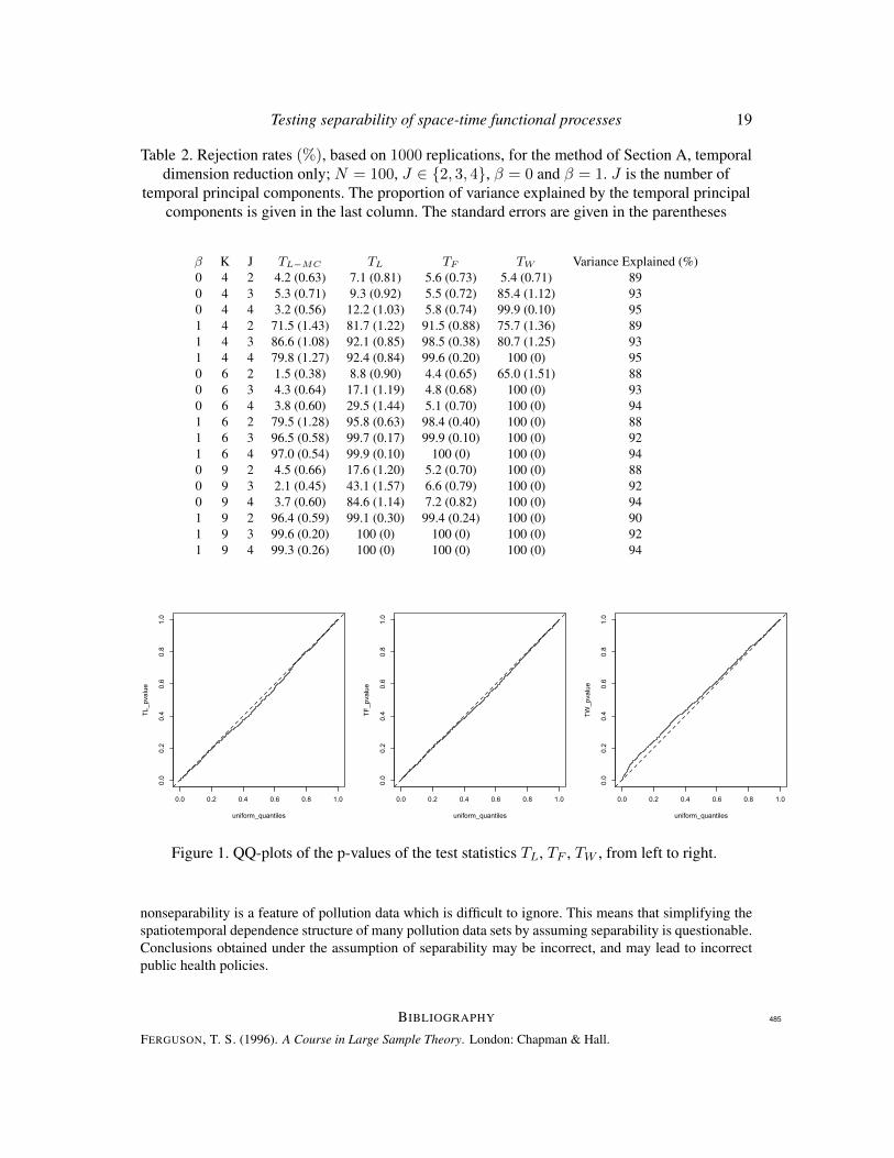
with all its health impacts, as well as impacts on both terrestrial and aquatic ecosystems.We consider nine locations that have relatively complete records since 2000: Allentown, Baltimore,
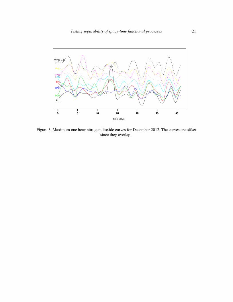
Boston, Harrisburg, Lancaster, New York City, Philadelphia, Pittsburgh, and Washington D.C. We usethe data for the years 2000-2012 . Each functional observation Xn(sk, t) consists of the daily maximumone-hour nitrogen dioxide concentration measured in ppb, parts per billion, for day t, month n, N = 156,475
and at location sk. Figure 3 shows the data for the nine locations for December 2012.Applying the tests to the deseasonalized curves obtained after removing the monthly mean from each
curve, as we did for the Irish wind data, we obtained p-values smaller than 0.001 for all L, J ∈ {2, 3, 4, 5}.In addition since the number of spatial locations is relatively small, only 9 stations, we applied our testswithout taking dimension reduction in space. Again, we obtained p-values smaller than 0.001. We see that480
Testing separability of space-time functional processes 19
Table 2. Rejection rates (%), based on 1000 replications, for the method of Section A, temporaldimension reduction only; N = 100, J ∈ {2, 3, 4}, β = 0 and β = 1. J is the number of
temporal principal components. The proportion of variance explained by the temporal principalcomponents is given in the last column. The standard errors are given in the parentheses
β K J TL−MC TL TF TW Variance Explained (%)0 4 2 4.2 (0.63) 7.1 (0.81) 5.6 (0.73) 5.4 (0.71) 890 4 3 5.3 (0.71) 9.3 (0.92) 5.5 (0.72) 85.4 (1.12) 930 4 4 3.2 (0.56) 12.2 (1.03) 5.8 (0.74) 99.9 (0.10) 951 4 2 71.5 (1.43) 81.7 (1.22) 91.5 (0.88) 75.7 (1.36) 891 4 3 86.6 (1.08) 92.1 (0.85) 98.5 (0.38) 80.7 (1.25) 931 4 4 79.8 (1.27) 92.4 (0.84) 99.6 (0.20) 100 (0) 950 6 2 1.5 (0.38) 8.8 (0.90) 4.4 (0.65) 65.0 (1.51) 880 6 3 4.3 (0.64) 17.1 (1.19) 4.8 (0.68) 100 (0) 930 6 4 3.8 (0.60) 29.5 (1.44) 5.1 (0.70) 100 (0) 941 6 2 79.5 (1.28) 95.8 (0.63) 98.4 (0.40) 100 (0) 881 6 3 96.5 (0.58) 99.7 (0.17) 99.9 (0.10) 100 (0) 921 6 4 97.0 (0.54) 99.9 (0.10) 100 (0) 100 (0) 940 9 2 4.5 (0.66) 17.6 (1.20) 5.2 (0.70) 100 (0) 880 9 3 2.1 (0.45) 43.1 (1.57) 6.6 (0.79) 100 (0) 920 9 4 3.7 (0.60) 84.6 (1.14) 7.2 (0.82) 100 (0) 941 9 2 96.4 (0.59) 99.1 (0.30) 99.4 (0.24) 100 (0) 901 9 3 99.6 (0.20) 100 (0) 100 (0) 100 (0) 921 9 4 99.3 (0.26) 100 (0) 100 (0) 100 (0) 94
0.0 0.2 0.4 0.6 0.8 1.0
0.0
0.2
0.4
0.6
0.8
1.0
uniform_quantiles
TL_pvalue
0.0 0.2 0.4 0.6 0.8 1.0
0.0
0.2
0.4
0.6
0.8
1.0
uniform_quantiles
TF_pvalue
0.0 0.2 0.4 0.6 0.8 1.0
0.0
0.2
0.4
0.6
0.8
1.0
uniform_quantiles
TW_pvalue
Figure 1. QQ-plots of the p-values of the test statistics TL, TF , TW , from left to right.
nonseparability is a feature of pollution data which is difficult to ignore. This means that simplifying thespatiotemporal dependence structure of many pollution data sets by assuming separability is questionable.Conclusions obtained under the assumption of separability may be incorrect, and may lead to incorrectpublic health policies.
BIBLIOGRAPHY 485
FERGUSON, T. S. (1996). A Course in Large Sample Theory. London: Chapman & Hall.
20 P. CONSTANTINOU, P. KOKOSZKA AND M. REIMHERR
0 5 10 15 20 25 30
time (days)
RPT
0 5 10 15 20 25 30
VAL
0 5 10 15 20 25 30
KIL
0 5 10 15 20 25 30
SHA
0 5 10 15 20 25 30
BIR
0 5 10 15 20 25 30
DUB
0 5 10 15 20 25 30
CLA
0 5 10 15 20 25 30
MUL
0 5 10 15 20 25 30
CLO
0 5 10 15 20 25 30
BEL
0 5 10 15 20 25 30
MAL
Figure 2. Irish wind speed curves for January 1961. Each curve corresponds to a differentlocation. The curves are offset since they overlap.
GNEITING, T. (2002). Nonseparable, stationary covariance functions for space–time data. Journal of the AmericanStatistical Association 97, 590–600.
HASLETT, J. & RAFTERY, A. E. (1989). Space–time modelling with long–memory dependence: Assesing Ireland’swind power resource (with discussion). Applied Statistics 38, 1–50.490
HORVATH, L. & KOKOSZKA, P. (2012). Inference for Functional Data with Applications. New York: Springer.MOORE, J. T., B. M. SADLER, B. M. & KOZICK, R. J. (2008). Maximum-likelihood estimation, the Cramer–
Rao bound, and the method of scoring with parameter constraints. IEEE Transactions on Signal Processing 56,895–908.
RAMSAY, J. O., HOOKER, G. & GRAVES, S. (2009). Functional Data Analysis with R and MATLAB. New York: 495
Springer.
[Received month year. Revised month year]
Testing separability of space-time functional processes 21
0 5 10 15 20 25 30
time (days)
ALL
0 5 10 15 20 25 30
BAL
0 5 10 15 20 25 30
BOS
0 5 10 15 20 25 30
HAR
0 5 10 15 20 25 30
LAN
0 5 10 15 20 25 30
NYC
0 5 10 15 20 25 30
PHI
0 5 10 15 20 25 30
PIT
0 5 10 15 20 25 30
WAS D.C
Figure 3. Maximum one hour nitrogen dioxide curves for December 2012. The curves are offsetsince they overlap.