Embed Size (px)
Citation preview

Supplementary Material for “Genotype, haplotype, and copy-numbervariation in worldwide human populations”
Contents
1 Preparation of SNP data 21.1 Overview . . . . . . . . . . . . . . . . . . . . . . . . . . . . . . . . . . . . . . . . . . . . . . . 21.2 Genotyping . . . . . . . . . . . . . . . . . . . . . . . . . . . . . . . . . . . . . . . . . . . . . . 21.3 Initial quality control . . . . . . . . . . . . . . . . . . . . . . . . . . . . . . . . . . . . . . . . . 21.4 Individuals . . . . . . . . . . . . . . . . . . . . . . . . . . . . . . . . . . . . . . . . . . . . . . 31.5 Populations . . . . . . . . . . . . . . . . . . . . . . . . . . . . . . . . . . . . . . . . . . . . . . 31.6 SNPs . . . . . . . . . . . . . . . . . . . . . . . . . . . . . . . . . . . . . . . . . . . . . . . . . . 41.7 Missing data rate . . . . . . . . . . . . . . . . . . . . . . . . . . . . . . . . . . . . . . . . . . . 51.8 Genotyping error rate . . . . . . . . . . . . . . . . . . . . . . . . . . . . . . . . . . . . . . . . 5
2 Population-genetic analysis of unphased SNP genotype data 52.1 Allele frequencies . . . . . . . . . . . . . . . . . . . . . . . . . . . . . . . . . . . . . . . . . . . 52.2 Linkage disequilibrium . . . . . . . . . . . . . . . . . . . . . . . . . . . . . . . . . . . . . . . . 52.3 Geographic distribution . . . . . . . . . . . . . . . . . . . . . . . . . . . . . . . . . . . . . . . 62.4 Structure . . . . . . . . . . . . . . . . . . . . . . . . . . . . . . . . . . . . . . . . . . . . . . . 62.5 Population tree . . . . . . . . . . . . . . . . . . . . . . . . . . . . . . . . . . . . . . . . . . . . 62.6 Multidimensional scaling . . . . . . . . . . . . . . . . . . . . . . . . . . . . . . . . . . . . . . . 72.7 Genetic and geographic distance . . . . . . . . . . . . . . . . . . . . . . . . . . . . . . . . . . 7
3 Preparation of haplotype data 73.1 Haplotype estimation with geographic region labels . . . . . . . . . . . . . . . . . . . . . . . . 73.2 Haplotype datasets for analysis of population structure . . . . . . . . . . . . . . . . . . . . . . 7
4 Population-genetic analysis of haplotype data 74.1 Linkage disequilibrium . . . . . . . . . . . . . . . . . . . . . . . . . . . . . . . . . . . . . . . . 74.2 Joint distribution of haplotype length and frequency . . . . . . . . . . . . . . . . . . . . . . . 84.3 A model for local clustering of haplotypes . . . . . . . . . . . . . . . . . . . . . . . . . . . . . 84.4 Haplotype cluster plots . . . . . . . . . . . . . . . . . . . . . . . . . . . . . . . . . . . . . . . . 94.5 Geographic distribution . . . . . . . . . . . . . . . . . . . . . . . . . . . . . . . . . . . . . . . 104.6 Structure . . . . . . . . . . . . . . . . . . . . . . . . . . . . . . . . . . . . . . . . . . . . . . . 104.7 Population tree . . . . . . . . . . . . . . . . . . . . . . . . . . . . . . . . . . . . . . . . . . . . 104.8 Multidimensional scaling . . . . . . . . . . . . . . . . . . . . . . . . . . . . . . . . . . . . . . . 10
5 Preparation of CNV data 115.1 Detecting CNVs using PennCNV . . . . . . . . . . . . . . . . . . . . . . . . . . . . . . . . . . . 115.2 Data cleaning . . . . . . . . . . . . . . . . . . . . . . . . . . . . . . . . . . . . . . . . . . . . . 115.3 False positives and false negatives . . . . . . . . . . . . . . . . . . . . . . . . . . . . . . . . . . 115.4 Summary of detected CNVs . . . . . . . . . . . . . . . . . . . . . . . . . . . . . . . . . . . . . 135.5 Duplications on the X chromosome in males . . . . . . . . . . . . . . . . . . . . . . . . . . . . 14
6 Population-genetic analysis of CNV data 146.1 Geographic distribution . . . . . . . . . . . . . . . . . . . . . . . . . . . . . . . . . . . . . . . 146.2 Structure . . . . . . . . . . . . . . . . . . . . . . . . . . . . . . . . . . . . . . . . . . . . . . . 146.3 Population tree . . . . . . . . . . . . . . . . . . . . . . . . . . . . . . . . . . . . . . . . . . . . 146.4 Multidimensional scaling . . . . . . . . . . . . . . . . . . . . . . . . . . . . . . . . . . . . . . . 14
7 Additional analysis of multiple data types 157.1 Linkage disequilibrium . . . . . . . . . . . . . . . . . . . . . . . . . . . . . . . . . . . . . . . . 157.2 Structure . . . . . . . . . . . . . . . . . . . . . . . . . . . . . . . . . . . . . . . . . . . . . . . 157.3 Population tree . . . . . . . . . . . . . . . . . . . . . . . . . . . . . . . . . . . . . . . . . . . . 167.4 Multidimensional scaling . . . . . . . . . . . . . . . . . . . . . . . . . . . . . . . . . . . . . . . 177.5 Genetic and geographic distance . . . . . . . . . . . . . . . . . . . . . . . . . . . . . . . . . . 17
1www.nature.com/nature 1

8 Comparative analysis of equal-sized SNP and CNV datasets 188.1 Reduced SNP datasets . . . . . . . . . . . . . . . . . . . . . . . . . . . . . . . . . . . . . . . . 188.2 Structure . . . . . . . . . . . . . . . . . . . . . . . . . . . . . . . . . . . . . . . . . . . . . . . 188.3 Population tree . . . . . . . . . . . . . . . . . . . . . . . . . . . . . . . . . . . . . . . . . . . . 188.4 Multidimensional scaling . . . . . . . . . . . . . . . . . . . . . . . . . . . . . . . . . . . . . . . 18
9 Supplementary tables and figures 19
References 64
1 Preparation of SNP data
1.1 Overview
The study design involved the high-resolution genotyping of a diverse sample of individuals at genome-widesingle-nucleotide polymorphisms (SNPs). The set of SNPs included SNPs spread across all autosomes, as wellas SNPs on the X chromosome, the pseudoautosomal region on the X and Y chromosomes, the nonrecombiningproportion of the Y chromosome, and the mitochondrion. The individuals genotyped were drawn from theHGDP-CEPH Human Genome Diversity Cell Line Panel1,2 (the “HGDP-CEPH panel” henceforth), and wereaugmented for some analyses with individuals taken from the International Haplotype Map Project3 (the“HapMap”). Following a series of quality control steps (Figure S17), an initial design using 513 HGDP-CEPHindividuals was reduced to a final dataset of 485 individuals and 525,910 genome-wide SNPs.
1.2 Genotyping
We selected a geographically broad collection of 513 HGDP-CEPH samples from 29 populations for geno-typing. DNA was derived from Epstein-Barr virus immortalized lymphocyte cell lines (LCL) maintainedas part of the HGDP-CEPH panel1. Genotyping was performed using Infinium HumanHap550 GenotypingBeadChips (Illumina Inc., San Diego, CA). Samples were assayed along with ongoing experiments in batchesof 48. For each sample, 1µg of DNA was used as template and the experiments were performed followingmanufacturer instructions. Our previous work has established that genetically, LCLs remain highly faithfulto the source tissue used for immortalization4.
Of the 513 samples, 316 were typed using HumanHap550 version 1 BeadChips and 197 were typed usingHumanHap550 version 3 BeadChips. Raw data from HumanHap550 version 1 and version 3 chips wereloaded as separate projects into Beadstudio version 3.1.4. Reclustering of SNP genotype calls was performed,discarding all genotypes below a no-call threshold of 0.15. All samples within each BeadStudio project(version 1 or version 3) were then reanalyzed using the newly derived genotype clusters.
1.3 Initial quality control
We generated a total of ∼275 million diploid genotypes in the 513 samples. After reclustering, 18 sampleswith a call rate <95% were permanently excluded from further analysis. The genotype call rate threshold of95% resulted in the removal of 13 samples typed on version 1 BeadChips and 5 samples typed on version 3BeadChips. The number of unique SNPs in common between version 1 and version 3 BeadChips is 545,066.To test genotype concordance across HumanHap550 version 1 and version 3 BeadChips, we genotyped bothBeadChip types in each of three replicate samples. Analysis of these replicates produced a mean genotypeconcordance rate of 0.999938 (range 0.999909 to 0.999954); the average number of called genotypes acrossreplicates was 539,161 of 545,066 attempted (range 538,112 to 540,476), and the average number of discordantcalls was 33 (range 25 to 46).
A locus-specific genotype call rate threshold of 98% (after reclustering) resulted in the removal of 18,667 ofthe 545,066 SNPs; thus 526,399 unique SNPs were successfully typed across 495 samples. The mean genotypecall rate across these samples was 99.75% after reclustering (range 96.24% to 99.95%; median 99.86%). Post-reclustering call rates were extremely high in most individuals (Figures S18 and S19), exceeding 98% in allexcept seven cases and exceeding 99% in all except 17 cases.
At this point, two HGDP-CEPH samples — a Palestinian and a Papuan — were discarded. On the basisof a comparison of an initial version of our genotypes to data on 122 SNPs from Conrad et al.5, these sampleswere suspected of having been mislabeled during the course of our project. Data preparation proceededusing the remaining 493 HGDP-CEPH samples and 526,399 SNPs, incorporating genotypes of 112 HapMapindividuals previously genotyped by Illumina (using version 1 BeadChips).
2www.nature.com/nature 2
1.4 Individuals
HGDP-CEPH panel. To verify the identities of the 493 remaining HGDP-CEPH individuals, we firstverified that sex inferred on the basis of X-chromosomal heterozygosity and Y-chromosomal missing datamatched the sex previously reported for each individual1,6. All individuals previously reported as male hadat most 2.05% heterozygous SNPs on the X chromosome and at most 2 of 10 SNPs with missing data on theY chromosome, whereas all individuals previously reported as female had at least 11.74% heterozygous SNPson the X chromosome and at least 5 of 10 SNPs with missing data on the Y chromosome (at least 9 of 10 inall except two cases).
We then compared genotypes at 122 autosomal SNPs that overlapped with the study of Conrad et al.5
Each of 1039 HGDP-CEPH individuals from the Conrad et al.5 dataset was compared with each of 493 HGDP-CEPH individuals genotyped in the current study. Except for four individuals that were not genotyped byConrad et al.5 (Adygei 1383, Adygei 1384, Biaka Pygmy 980, Russian 890), for each individual typed in thecurrent study, the genotypes of the 122 SNPs obtained using Illumina BeadChips almost exactly matchedthose associated by Conrad et al.5 with the same individual label (or its duplicate, in cases where only onemember of a duplicate pair was genotyped by Conrad et al.5). In some cases, up to 2 of the 122 SNPs had adiscrepancy in which one dataset produced a heterozygote and the other produced a homozygote. However,other than known duplicates and pairs with the same individual label, no other pairs of individuals involvinggenotypes from the Conrad et al.5 study and genotypes from the current study had more than 87% of SNPsin which both alleles agreed. Because the only pairs of individuals with a high level of genotype concordancebetween studies were those expected on the basis of identical individual labels, it was assumed that no newsample labeling errors or sample duplicates occurred in any of the 493 HGDP-CEPH samples since the timeof the earlier Conrad et al.5 study.
HapMap. For all 112 HapMap individuals, sex information inferred on the basis of X-chromosomal heterozy-gosity and Y-chromosomal missing data (using the same criteria as for the HGDP-CEPH samples) matchedthe previously reported sex. The sample from the HapMap did not contain any two individuals found bythe HapMap Consortium3 in their Supplementary Table 15 to have an “unreported relationship,” althoughit did contain two Japanese individuals inferred to have relatively high inbreeding coefficients. Included aspart of the HapMap sample were 28 parent/parent/offspring trios — 16 from the CEU sample, and 12 fromthe YRI sample. For all pairs of individuals in the HapMap sample, computations of P0, P1, and P2 — thefractions of autosomal SNPs with 0, 1, and 2 alleles shared identical in state — were used to verify thatrelative pairs matched those expected3. This computation utilized 7734 SNPs on chromosome 21. For allparent/parent/offspring trios previously reported, parent/offspring relationships were in fact inferred betweenthe offspring in each trio and each of the two parents (P0 < 0.0006 for each parent/offspring pair), and noother parent/offspring relationships involving two HapMap samples were identified (P0 > 0.04 for all otherpairs). No two HapMap individuals were found to be sample duplicates (P2 < 0.73 for all pairs).
Final set of individuals. The sample of 493 HGDP-CEPH individuals included seven pairs of duplicatesamples; for each duplicate pair the individual not in the H1048 subset of the HGDP-CEPH panel6 wasexcluded from the final set for data analysis (Druze 589, Bedouin 652, Melanesian 659, Melanesian 826,Biaka Pygmy 981, Biaka Pygmy 1087, and Biaka Pygmy 1092). Biaka Pygmy 980 was also excluded due to apreviously reported labeling error6,7. The final set of individuals for data analysis included 485 HGDP-CEPHand 112 HapMap individuals.
The set of 485 HGDP-CEPH individuals included 440 individuals from the H952 subset, which containsno first- or second-degree relatives6. Among the relatives, four parent/parent/offspring trios were included:Melanesian 655 (father), 656 (mother), and 657 (daughter); Melanesian 788 (father), 660 (mother), and 789(son); Melanesian 788 (father), 660 (mother), and 824 (son); Pima 1037 (father), 1038 (mother), and 1039(son). Analyses that excluded relatives were restricted to 84 HapMap individuals — excluding offspring fromtrios — and 443 HGDP-CEPH individuals. The HGDP-CEPH set of “unrelated” individuals included the440 individuals from the H952 set without close relatives6, together with Pima individuals 1046 and 1049 andMaya 866. These three individuals were retained, as none of their close relatives were among the individualsgenotyped (or, in the case of Maya 866, the close relative that if genotyped would have led to her exclusionwas not genotyped). Sample sizes for the various populations are displayed in Table S5.
1.5 Populations
The populations studied are shown on the map in Figure S1 at the coordinates used in Rosenberg et al.8.These coordinates (Table S6) match those of Cann et al.1, except that an averaging procedure was used forpopulations given by Cann et al.1 with a range for the latitudes and longitudes, and an updated location
3www.nature.com/nature 3
was used for Mongola. Populations were classified by geographic region in the same manner as in previouswork with the same individuals7. For some analyses, the geographic regions of Europe, Middle East, andCentral/South Asia were grouped into a “Eurasia” region. “Africa” refers to Sub-Saharan Africa. TheHapMap Chinese (CHB) and Japanese (JPT) samples were included with East Asia; HapMap Yoruba (YRI)individuals were included with Africa, and HapMap European Americans (CEU) were included with Europe.
1.6 SNPs
After the set of individuals was established, apparent heterozygotes among males for X-chromosomal lociwere recoded as missing data, as were heterozygotes at mitochondrial SNPs and non-missing Y-chromosomalgenotypes among females. Similar procedures to those of Conrad et al.5 were then applied to remove SNPswith lower quality data. Separate quality checks were applied to the recoded dataset, and upon completionof all checks, those SNPs that did not pass any one of the tests were excluded.
Monomorphic SNPs. In the final set of 597 individuals used in data analysis (485 HGDP-CEPH and 112HapMap), 42 monomorphic SNPs were identified. The remaining SNPs included 48,723 AC, 214,444 AG,214,751 CT, and 48,439 GT polymorphisms.
SNPs with missing data. Considering the set of 527 unrelated individuals (443 HGDP-CEPH and 84HapMap), 161 SNPs with at least 10% missing data were identified. For autosomal, pseudoautosomal, andmitochondrial SNPs, the fraction of missing data was calculated as the total fraction of individuals whosegenotypes were missing. For X-chromosomal loci, it was equal to (2f ′+m′)/(2f +m), where f , m, f ′, and m′
respectively denote the number of females considered (202), the number of males considered (325), the numberof females with missing genotypes, and the number of males with missing genotypes. For Y-chromosomalSNPs, the missing data rate was calculated as the fraction of males whose genotypes were missing.
SNPs were also identified for which one or more populations had a sample size of fewer than 5 alleles inthe sample of 527 unrelated individuals. This criterion, which was not applied to the Y chromosome or themitochondrial genome, led to the identification of 135 SNPs — six autosomal and 129 X-chromosomal SNPs.
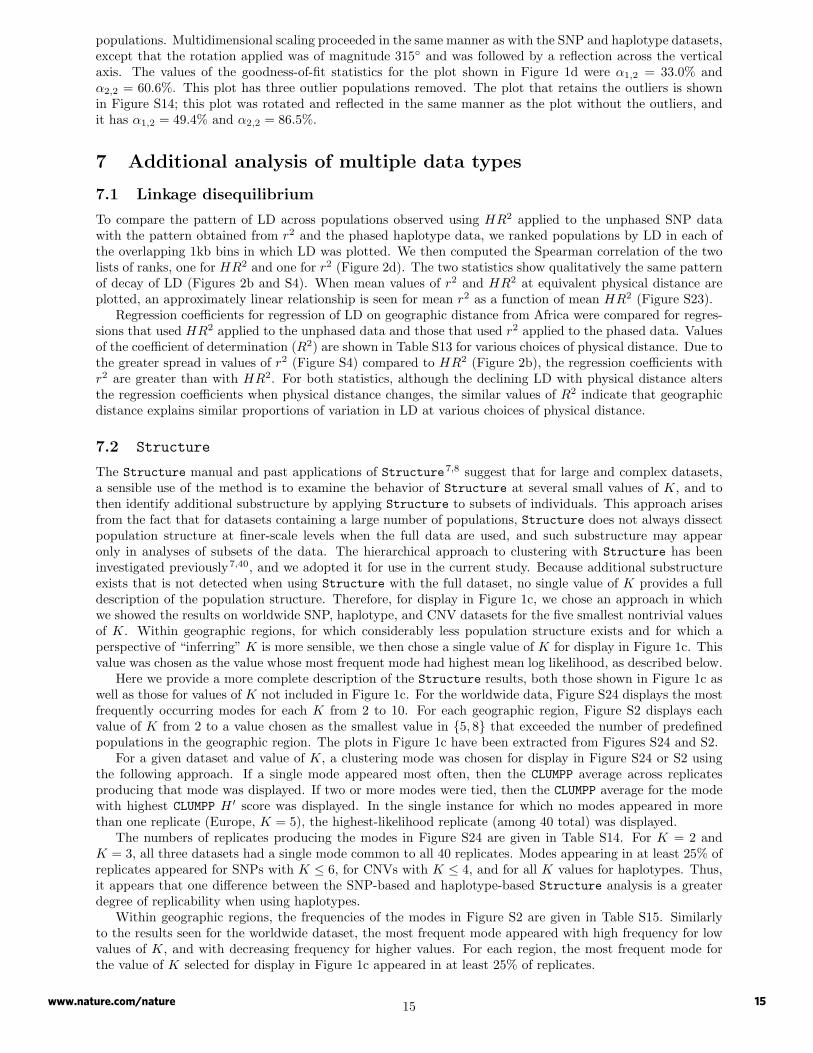
SNPs not in Hardy-Weinberg equilibrium. From the set of 527 unrelated individuals, two populationgroupings with relatively low levels of population structure in previous work7 were constructed: a MiddleEast group consisting of Bedouin, Druze, and Palestinian samples (107 individuals), and a sub-Saharan Africagroup consisting of the Bantu (Southern Africa), Bantu (Kenya), Mandenka, and Yoruba populations (63individuals).
A chi-squared test of the null hypothesis of Hardy-Weinberg equilibrium was performed in each of thesepopulation groups, taking into account the Yates continuity correction9. For X-chromosomal SNPs, maleswere included in the tabulation of allele frequencies for the computation of expected genotype frequencies,but they were ignored in the hypothesis test. Only SNPs with at least four copies of the minor allele inboth of the population groups were considered as possible candidates for exclusion. Among such SNPs, thoseSNPs that had either or both of the following properties were identified: (1) the chi-squared test statisticwas greater than 19.51142 (P < 10−5 for a χ2
1 distribution) in either of the two population groups; (2) thechi-squared test statistic was greater than 6.634897 (P < 10−2 for a χ2
1 distribution) in both of the populationgroups (Figure S20). Using these criteria, 198 SNPs were identified.
SNPs discordant between duplicates. For each SNP, concordance of genotypes was evaluated betweenthe two individuals in each duplicate pair. For all SNPs, non-identical genotypes in which neither individualhad missing data were declared discordant. Two SNPs were identified in which two of the seven duplicatepairs had discordant genotypes.
SNPs with Mendelian incompatibilities. For each of the 32 trios (4 HGDP-CEPH, 16 HapMap CEU,and 12 HapMap YRI), SNPs were tested for Mendelian incompatibilities. A total of 26 SNPs with at leastthree Mendelian incompatibilities among the 32 trios were identified.
Summary of excluded SNPs. Not taking into account the fact that some SNPs failed more than oneof the checks, the total number of SNPs identified by the various quality checks was 564 — 42 that weremonomorphic, 161 with a high overall missing data date, 135 with considerable missing data in at least onepopulation, 198 with Hardy-Weinberg disequilibrium, 2 with discordance between duplicates, and 26 withMendelian incompatibilities. Accounting for SNPs that failed more than one of the quality checks, 489 distinctSNPs were identified and were discarded from the final dataset for analysis. Excluding these SNPs, the SNPset for data analysis included 525,910 SNPs — 512,762 autosomal, 13,052 X-chromosomal, 9 Y-chromosomal,15 pseudoautosomal, and 72 mitochondrial SNPs (Table S7).
4www.nature.com/nature 4

1.7 Missing data rate
Of the 2(597)(512, 762) = 612, 237, 828 autosomal genotypes possible in the full sample of 597 individuals,the number of missing genotypes was 759,570. Similarly, the proportions of missing genotypes for the Ychromosome, the pseudoautosomal region, and the mitochondrial genome were 48 of 3285, 92 of 17,910, and1194 of 42,984 possible genotypes. Of the (365 + 2 × 232)(13, 052) = 10, 820, 108 X-chromosomal genotypespossible, the number missing was 36,982. Combining all 525,910 SNPs, the missing data rate was
759, 570 + 48 + 92 + 1194 + 36, 982612, 237, 828 + 3285 + 17, 910 + 42, 984 + 10, 820, 108
=797, 886
623, 122, 115≈ 0.13%.
Most individuals and SNPs had a very low missing data rate (Tables S8 and S9). None of the individualshad more than 3.5% missing data, as determined using all 525,910 SNPs.
1.8 Genotyping error rate
A rate of genotype discrepancy was determined based on duplicate samples, using 513,008 autosomal SNPs(prior to removal of 246 autosomal SNPs that failed quality checks). Considering autosomal SNPs for whichboth individuals in a duplicate pair were genotyped, 174 discrepancies were observed in which one individualwas homozygous and the other was heterozygous, and 1 discrepancy was observed in which the two indi-viduals were homozygous for different alleles. Therefore, the rate of discrepancies per diploid genotype was175/3, 580, 862 ≈ 4.92× 10⁻⁵.
Comparing the genotypes at the overlapping 122 SNPs to the data from Conrad et al.5, there were 482individuals who were genotyped in both studies (not counting seven cases in which one study contained theduplicate cell line of an individual but not the identical cell line). Excluding comparisons in which one studyproduced missing data, the rate of discrepancies between studies per diploid genotype was 54/57, 764 ≈9.35× 10⁻⁴. This rate is somewhat higher than the discordance rate for duplicate cell lines genotyped in thepresent study, but note that the Conrad et al.5 study used a different genotyping technology.
2 Population-genetic analysis of unphased SNP genotype data
2.1 Allele frequencies
For comparisons of SNP allele frequencies between geographic regions, we used the 443 unrelated HGDP-CEPH individuals and the 512,762 autosomal SNPs. To produce bivariate graphs of allele frequencies in twogeographic regions (Figure S21A), we plotted the number of SNPs with minor allele frequency in each of aseries of bins. We employed a resampling procedure to adjust for sample size differences among geographicregions. For each SNP, we sampled 40 alleles (with replacement) from each of the geographic regions. For agiven pair of regions, the minor allele was identified from the pooled sample of 80 alleles for the two regions. Incases where both alleles had exactly 40 copies in the combined sample, the minor allele was chosen randomly.The numbers of SNPs in each of the 41 × 42/2 = 861 possible bivariate frequency categories were thentabulated. To obtain values proportional to SNP density per unit area, for triangular bins along the diagonal(frequency sum of one for the two population groups), this number of SNPs was doubled to account for thearbitrary decision about which allele was the minor allele and to account for the fact that the triangular binshad only half the area of usual square bins. Univariate allele frequency spectra (Figure S21B) were basedon the same resamples as those used in producing the bivariate spectra. Correlation coefficients of allelefrequencies, obtained based on the values plotted but using both alleles at each SNP, are shown in Table S10.
2.2 Linkage disequilibrium
Linkage disequilibrium (LD) was measured for the unphased data using the HR2 statistic10, a measureanalogous to the r2 statistic for phased data that for a pair of SNPs considers a normalized squared differencebetween the proportion of double homozygotes expected under linkage equilibrium and the proportion ofdouble homozygotes observed. For each population, we computed HR2 for all pairs of autosomal SNPs withphysical distance <70.5kb. We used a resampling procedure to adjust for possible influence of sample sizeon homozygosity-based LD statistics11. For each pair of SNPs, a random set of five individuals was sampledwithout replacement in each population, and the LD computation was performed using those five individuals(ignoring missing data among the five individuals). Pairs of SNPs in which the five individuals chosen weremonomorphic at one or both SNPs were excluded from the computation. In the computations of HR2, thehomozygosity of a locus was obtained using all individuals who had genotypes present at the locus, while the
5www.nature.com/nature 5

double homozygosity for a pair of loci was obtained considering all individuals who had genotypes presentat both loci. As certain missing data configurations can produce HR2 > 1 with this approach, a smallproportion of values of HR2 that exceeded 1 were set to 1.
SNP pairs were placed in bins of size 250bp (including the lower endpoint in the bin). For each population,starting at 500bp, the mean HR2 value in 1kb windows was computed every 250 base pairs. As an example,the value plotted at 10kb in Figure 2b (and 2c) is the mean HR2 for all SNP pairs with physical distance in[9500,10500). The standard error plotted in Figure 2c is obtained using this same collection of pairs of SNPs.
Regression of LD on geographic distance from East Africa was performed using mean HR2 values forparticular physical distance bins. Geographic distance was computed using the approach of Rosenberg etal.8, starting from Addis Ababa (9◦N 38◦E) and traveling along the waypoint routes of Ramachandran etal.12. Paths involving the Americas all passed through 64◦N 177◦E and 54◦N 130◦W, paths involving Oceaniapassed through 11◦N 104◦E, and paths involving Africa (including the Mozabite population) passed through30◦N 31◦E. Paths from Europe (excluding Adygei) to Africa, the Middle East (excluding Mozabites), orOceania also passed through 41◦N 28◦E.
2.3 Geographic distribution
We used the rarefaction approach to assess the distributions of alleles across geographic regions while adjustingfor differing sample sizes13. This method, which extends the rarefaction formula of Kalinowski14 for privateallelic richness, examines the mean number of alleles with each of a set of possible geographic distributions,considering all possible subsamples with equal size g from each of the geographic regions. The analysis usedthe 443 unrelated individuals and 512,509 autosomal SNPs, omitting those SNPs with >10% missing data inany of the five major geographic regions. The omission of SNPs with >10% missing data made it possible toconsider larger values of the standardized sample size g. The proportions of SNPs with particular geographicdistributions were obtained by averaging estimates across loci at g = 35.
2.4 Structure
The Bayesian clustering software Structure15,16 was used to cluster individuals using their SNP genotypes.Replicate Structure runs used a burn-in period of 20,000 iterations followed by 10,000 iterations from whichestimates were obtained. All runs were based on the admixture model, in which each individual is assumedto have ancestry in multiple genetic clusters, using the F model of correlation in allele frequencies acrossclusters. Graphs of Structure results were produced using Distruct17.
This analysis used the 443 HGDP-CEPH unrelated individuals, as well as subsets of this collection cor-responding to individual geographic regions. Four SNP subsets were obtained, each containing ∼1% of theautosomal SNPs. Chromosomes were placed in numerical order, and SNPs were ordered on each chromosomeusing the build 36.2 human genome sequence (dbSNP build 127). With SNPs ordered from 1 to 512,762, thefour subsets consisted of SNPs in numbered positions 1 mod 100, 26 mod 100, 51 mod 100, and 76 mod 100.
For a given subset of individuals and value of K, the number of clusters considered, ten replicate analyseswith Structure were performed for each 1% collection of SNPs. The 40 replicates for each subset of individ-uals and each K were then analyzed with CLUMPP18 to identify common modes among the replicates, usinga procedure similar to that of Wang et al.19. CLUMPP analysis proceeded using the LargeKGreedy algorithmwith 10,000 random permutations. A set of runs was classified as characterizing a single mode if all pairs inthe set had a symmetric similarity coefficient G′ > 0.9. Note that because of possible nontransitivity of thecriterion G′ > 0.9, it sometimes occurred that a run was considered part of two or more distinct modes.
For each mode identified, we ran CLUMPP a second time (using the LargeKGreedy algorithm and 10,000random permutations), using only the replicates belonging to the mode. From this analysis, for each mode, weobtained the mean across replicates of the cluster membership coefficients of each individual. For each subsetof individuals and each value of K, we identified the most frequently occurring mode, breaking ties using theCLUMPP H ′ score. We also obtained mean log likelihood scores across replicates in the most frequent mode.Further details regarding the Structure and CLUMPP analyses, including additional results and a descriptionof the basis for selecting some of these results for display in Figure 1c, are provided in Section 7.2.
2.5 Population tree
A neighbor-joining tree of populations20 was obtained based on pairwise allele-sharing distance among pop-ulations. This analysis used 512,762 autosomal SNPs and the 443 unrelated individuals. Confidence valueswere obtained using 1000 bootstrap resamples across loci. The computation of bootstrap distances was per-formed using microsat21, and the tree was obtained using the neighbor, consense, and drawtree programs
6www.nature.com/nature 6
in the phylip package22. The production of the consensus tree used extended majority rule consensus (greedyconsensus23), as implemented in consense. External branches are drawn with equal lengths, and internalbranch lengths are proportional to bootstrap support.
2.6 Multidimensional scaling
A matrix of pairwise distances was constructed for the 443 unrelated HGDP-CEPH individuals, using the512,762 autosomal SNPs. Between-individual distances were obtained using allele-sharing distance, P0+P1/2,where Pk represents the proportion of loci at which the individuals shared exactly k alleles identical instate. The overall distance between individuals was obtained as the average across loci. Classical metricmultidimensional scaling24,25 was applied to the individual distance matrix to provide a representation of thematrix in two dimensions. The resulting coordinates were then rotated 225◦ to place the populations in anapproximate geographic orientation. This analysis utilized the cmdscale function in R25. Two goodness-of-fitcriteria for the proportion of the distance matrix explained by the MDS scaling are α1,2 and α2,2 (eqs. 14.4.7and 14.4.8 of Mardia et al.24). For the plot shown for SNP data, α1,2 = 19.5% and α2,2 = 88.7%.
2.7 Genetic and geographic distance
We analyzed the relationship of genetic and geographic distance for pairs of populations. For the 512,762autosomal SNPs, genetic distance was computed with FST , using eq. 5.3 of Weir9. Geographic distancebetween populations used the same waypoint routes as were used in Section 2.2.
3 Preparation of haplotype data
3.1 Haplotype estimation with geographic region labels
Haplotypes and missing genotypes were estimated with fastPHASE26 version 1.3, ordering SNPs on eachchromosome according to positions from build 36.2 of the human genome sequence. As in Conrad et al.5, forestimating haplotypes and missing genotypes, geographic region labels (Table S5) were applied during themodel fitting procedure to enhance accuracy (“population labels” in Scheet & Stephens26). The number ofhaplotype clusters was set to 20, and we employed the default setting of 20 runs of the EM algorithm. Thisanalysis was used to generate a “best guess” estimate of the true underlying patterns of haplotype structure.
We included all 597 available individuals during haplotype estimation (485 HGDP-CEPH and 112 HapMap).This combined sample included related individuals; however, during haplotype estimation and model fitting(Section 4.3), we treated all individuals as unrelated. Haplotype phase was estimated for all autosomes aswell as for the pseudoautosomal region; for the X chromosome the haplotype estimation procedure treatedmales as having known haplotype. As described below, we removed relatives from the phased haplotype datato create a dataset of 527 unrelated individuals (443 HGDP-CEPH and 84 HapMap).
The “best guess” estimate of haplotype structure was used in the analyses of LD (Section 4.1) and ofhaplotype length and frequency (Section 4.2), as well as in the plots of haplotype structure (Section 4.4).
3.2 Haplotype datasets for analysis of population structure
To generate haplotype datasets for analyses of population structure (geographic distribution of haplotypes,Structure, population tree, and multidimensional scaling) we performed additional fastPHASE model fittingwithout using the geographic labels. For these analyses, we wanted to make inferences regarding populationstructure, rather than leverage a known or assumed structure for more accurate genotype estimation. Asabove, we included all 597 available individuals for model fitting, only afterwards removing relatives. Theprocedure for generating the haplotype datasets for population structure analyses is described in Section 4.3.
4 Population-genetic analysis of haplotype data
4.1 Linkage disequilibrium
LD was measured from the haplotype data using the r2 statistic27. This analysis used the autosomal haplotypeestimates, restricting attention to unrelated individuals. For each population, we computed r2 for all pairs ofautosomal SNPs with physical distance <70.5kb. Analogously to the computation of HR2 for the unphaseddata, we used a resampling procedure to adjust for possible influence of sample size on r2. For each pair ofSNPs, a random set of ten haplotypes was chosen in each population, and the LD computation was performed
7www.nature.com/nature 7

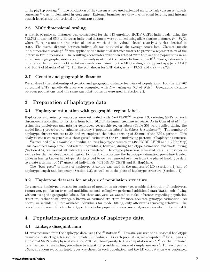
using those ten haplotypes. Pairs of SNPs in which the ten haplotypes chosen were monomorphic at one orboth SNPs were excluded from the computation. SNP pairs were placed in overlapping bins in the samemanner as in the HR2 computations for unphased data, and the mean was taken for each bin. The decay ofmean r2 with physical distance is plotted in Figure S4. Regression of LD on geographic distance from EastAfrica was performed using r2 values in the same manner as in the regressions involving HR2.
4.2 Joint distribution of haplotype length and frequency
Two haplotype properties that are inherently connected are the length of a haplotype and the frequency ofthat haplotype. Long haplotypes tend to have lower frequencies than do short haplotypes. To assess both ofthese properties simultaneously without applying predefined window sizes of haplotype lengths, we devised amethod that computes the length of every observed haplotype as well as its corresponding frequency.
For this analysis, we used the “best guess” phased data for 527 unrelated HGDP-CEPH and HapMapindividuals, analyzing the whole autosomal genome. Let the n SNPs of a given chromosome arm belong to theset S, where si denotes SNP i (i = 1, ..., n) and pi denotes the position of SNP si. The set S is ordered so thatpi < pi+1 and so that each SNP has two possible states, “0” and “1”. For the set of SNPs {si, ..., sj} (withi < j ≤ n), denote the set of possible haplotypes by hij . In this context a haplotype is defined as the seriesof states (0 or 1) along a specific chromosome, for some SNPs si to sj . If two chromosomes have identicalstates at all SNPs from si to sj , then the two chromosomes have identical haplotypes in [i, j]; otherwise, thechromosomes have different haplotypes. The number of possible haplotypes for the SNP set si, ..., sj is 2j−i+1;this number grows quickly as j − i + 1 increases, but in practice, the number of unique haplotypes that areobserved is relatively small. Denote the number of observed unique haplotypes for the set hij of haplotypesby Kij . For the SNP set {si, ..., sj}, each observed unique haplotype is denoted hijk, where k = 1, ...,Kij .
Starting from the first SNP s1, we move to SNP s2, and we compute (and store) the length in basepairs (`1,2 = p2 − p1 + 1) of the haplotypes in the set h1,2, and the frequencies of all haplotypes h1,2,k. Wethen proceed to SNP s3, and compute the length and frequency for all haplotypes h1,3,k. This procedure isrepeated for all sets of haplotypes h1,j , j = 2, ..., n (in practice, we truncate the calculation when the set ofobserved unique haplotypes has the same size as the number of sampled chromosomes — which occurs wellbefore the end of the chromosome). Thus, for i = 1, . . . , n − 1 and j = i + 1, . . . , n, we compute the lengthand the frequency for each haplotype hijk, which gives us the joint distribution of haplotype lengths andhaplotype frequencies without using window sizes to define haplotype length.
We computed the joint haplotype length and frequency distribution for each of the 29 HGDP-CEPHpopulations as well as for the 4 HapMap populations (Figure S5). To adjust for sample size differences acrosspopulations, in each population for each set of haplotypes hij , we performed the analysis using 12 randomlychosen chromosomes (sampled without replacement). For convenience, we ignored haplotypes of frequency 1of 12, so that the normalization used in computing the fraction of haplotypes that lie in a given length andfrequency bin is based only on haplotypes of frequency at least 2 of 12.
4.3 A model for local clustering of haplotypes
Motivation. Here we introduce a novel model-based approach for describing and displaying haplotypicvariation within and among populations. Our approach, which is based on the model underlying fastPHASE26,can be viewed as a summary of common haplotype frequencies in a sample.
In approaches to haplotype variation that consider windows of a given haplotype length (such as in Section4.1), haplotypes are first estimated, then they are binned within windows of a given size, with the choice ofwindow size having a sizeable effect on the haplotype frequency spectrum. In such analyses, it is important toinvestigate multiple haplotype lengths, as it may be difficult to determine the ideal window size for analysis.
An alternative approach for circumventing the issue of window size is to summarize variation using anLD model that locally captures the natural extent of haplotypes26. Over short physical distances, haplotypessampled from a population of chromosomes can be clustered into groups of similar haplotypes; these “haplo-type clusters” then summarize the overall variation in the population. Our approach enables the clusteringprocess to be applied to an entire chromosome by using a hidden Markov model for the underlying “haplo-type cluster” memberships of individual haplotypes in the sample. The model has been used previously forestimating haplotypes and missing genotypes, as implemented in the software package fastPHASE26.
Here we utilize the machinery of fastPHASE to obtain the frequencies of the latent haplotype clusters,which are represented by their cluster centers. These centers, or “fuzzy haplotypes,” represent locally thecommon haplotypes in a random sample of chromosomes from a population (or multiple populations). Useof these model-based cluster frequencies allows marker-wise summaries of haplotype variation to be producedin the form of the “frequency distribution” of haplotype clusters.
8www.nature.com/nature 8

The model. We recapitulate some notation from Scheet & Stephens26. We assume unphased individualmultilocus diploid genotypes g, observed at M SNP markers in n diploid individuals. We assume that thereare K haplotype clusters, which we estimate from the data. For convenience we set K equal to 20.
Let z·im denote the unobserved pair of haplotype cluster memberships for individual i at SNP marker
m. Let pmk(i) denote the relative frequency of haplotype cluster k (1, . . . ,K), in individual i at markerm (1, . . . ,M). To calculate pmk(i) we integrate over the possible pairs of cluster memberships, given theobserved data g and model parameters ν, as follows:
pmk(i) =
[∑Kk′=1 P
(z·im = {k, k′}|g, ν
)]+ P
(z·im = {k, k}|g, ν
)2
,
where P (z·im|g, ν) is given by Scheet & Stephens26. The quantities pmk(i) for k = 1, ...,K can be viewed as
the relative cluster frequencies for a very small population of chromosomes (of size 2). The integration overpossible pairs of cluster memberships amounts to integrating over uncertainty in haplotypic phase.
Now suppose that instead of a homogeneous sample of diploid individuals, we sample individuals from S
predefined “populations.” We can calculate p(s)mk, the relative frequency of cluster k in population s (1, . . . , S),
by averaging pmk(i) over members of this population as follows:
p(s)mk =
1ns
∑i∈Is
pmk(i).
In this equation, Is is the subset of individuals who belong to population s, and ns is the number of elementsin Is (that is, the sample size for population s). Calculation of P
(zi|g, ν
)can be accomplished efficiently
with a dynamic programming algorithm, and the parameters ν are estimated via an EM algorithm26.Once we have obtained the common haplotype frequencies {p(s)
mk} at a particular marker m, we can usethem to summarize the haplotype variation at that marker, within and among populations. Although we areassessing haplotype variation, and we are therefore inherently modeling genetic variation at multiple SNPssimultaneously, the information may be conveniently summarized pointwise at each marker, thus avoidingthe problem of choosing window sizes.
Sampling latent cluster memberships. Because the EM algorithm generally obtains local modes of thelikelihood P (g|ν), we run the EM algorithm T times, obtaining sets of parameter estimates (ν(1), . . . , ν(T )).From each of these parameter sets, we can sample an instantiation from the conditional distribution of thechromosome-wide list of cluster memberships z, given the estimated parameters and the observed genotypedata. An algorithm for sampling from P
(z|g, ν
)is given by Scheet & Stephens26.
For use in analyses of population structure, we generated a single sample of haplotype cluster membershipsfrom each of T = 10 model fittings (that is, ten independent runs of the EM algorithm). That is, we generatedten datasets so that at each SNP position across the genome, each individual was given a pair of haplotypecluster memberships, with each cluster membership equaling an integer ranging from 1 to 20. These datasetswere then analyzed in the same manner as one would analyze unphased multiallelic datasets. As noted above,the ten model fittings were obtained by treating the sample of individuals as homogeneous, rather than byusing S = 7 populations characterized by the geographic regions in Table S5.
4.4 Haplotype cluster plots
Figures 3 and S6 each contain visualizations of the haplotype cluster frequencies {p(s)mk} in the 527 unrelated
HGDP-CEPH and HapMap individuals, across different populations and geographic regions, for particularregions of the genome. Each plot is based on one of the 20 parameter estimate sets used to obtain the“best guess” haplotypes used in Sections 4.1 and 4.2. Within each box (corresponding to a population),cluster frequencies in the population are arranged vertically at consecutive SNPs. Each SNP is indicated by ahorizontal position, and the 20 colors indicate the frequencies for 20 haplotype clusters. No attempt is madeto model the degree of similarity among the different haplotypes represented by different clusters; thus, nomeaning is intended by the similarity or dissimilarity of the colors referring to different haplotype clusters.
Although it is difficult to visually ascertain exact haplotype cluster frequencies at individual SNPs, thegradual change in frequencies due to the gradual decay of LD allows the information at adjacent SNPs toblend together smoothly. One natural summary of each haplotype cluster visualization, which is largelycontinuous across each picture, is haplotype cluster homozygosity. We computed this homozygosity using thehaplotype cluster frequencies (treated as parametric frequencies), averaging across the ten haplotype clusterdatasets to obtain an overall estimate. For comparison, we also computed a standardized haplotype clusterhomozygosity for each population, subtracting the genome-wide mean haplotype cluster homozygosity andthen dividing by the standard deviation of haplotype cluster homozygosity across the genome (Figure S7).
9www.nature.com/nature 9

4.5 Geographic distribution
We used rarefaction13 on the ten imputations of the haplotype clusters, averaging results across imputationsto obtain the final estimates. This analysis was performed with the 443 unrelated HGDP-CEPH individualsin the same manner as for the SNP data. As the haplotype datasets contain no missing data, analysisof geographic distributions was performed at each autosomal locus, and results were averaged across loci.Rarefaction corrects for sample size only after production of haplotype datasets; sample size may have a smallinfluence during dataset production, as larger samples contribute more information during model fitting.
4.6 Structure
Analysis of imputed haplotype clusters using Structure and CLUMPP with 443 unrelated HGDP-CEPH in-dividuals proceeded in a similar manner to the analysis with unphased SNPs (using the G′ > 0.9 criterion).Each of the ten imputations of cluster memberships (one from each of the ten model fittings described above)was used in the Structure analysis. For each of the ten datasets, two subsets of the SNP data were obtained,each containing ∼1% of the autosomal SNPs. SNPs were ordered on each chromosome using the build 36.2human genome sequence, and separately on each chromosome, SNPs in numbered positions 1 mod 100 wereplaced in one subset, and SNPs in positions 51 mod 100 were placed in a second subset. A total of 40Structure runs were performed for each value of the model parameter specifying the number of clusters inthe Structure analysis — two replicates for each combination of one of the ten imputations and one of thetwo 1% subsets of SNPs. CLUMPP analysis was performed on these 40 replicates, in the same manner as forthe SNP dataset. Details of the results are described in Section 7.2.
4.7 Population tree
A neighbor-joining tree of populations was obtained based on the haplotype cluster membership data in thesame manner as with the SNP data, using the 443 unrelated HGDP-CEPH individuals. This analysis wasrestricted to every 10th SNP marker across the autosomes (on each chromosome, the SNPs chosen werethose in 1 mod 10 positions when enumerated according to the build 36.2 genome sequence, starting from 1).Confidence values were obtained by combining 1000 bootstrap-resampled distance matrices — 100 resamplesfor each of the same ten imputations used in the Structure analysis.
4.8 Multidimensional scaling
To generate a distance matrix for use in multidimensional scaling, we computed a “haplotype distance”between all pairs of individuals. We define dh
m(i, j) as the haplotype distance between the haplotype clusterprobability vectors for individuals i and j at marker m, calculated in the following manner:
dhm(i, j) =
√∑K
k=1(pmk(i)− pmk(j))2.
Finally, we obtained a haplotype genetic distance between individuals by averaging over multiple SNP markersand multiple model fittings.
Implicitly, pmk(i) is associated with a single model fit, or a single set of parameters ν. For producing theplots in Figure 1d, we calculated an average haplotype distance between all pairs of individuals by averagingdh
m(i, j) from every 10th SNP marker across the autosomes (on each chromosome, the SNPs chosen werethose in 1 mod 10 positions when enumerated according to the build 36.2 genome sequence, starting from1) over ten sets of model parameters (estimated from the same ten independent model fittings used in theStructure and population tree analyses). The final average haplotype distance was produced from
dh(i, j) =1
10|M|
10∑t=1
∑m∈M
dhm(i, j)t,
where M is the set containing every 10th autosomal SNP marker, |M| is the number of elements in this set,and dh
m(i, j)t represents the haplotype distance calculated from EM run t (1, . . . , 10).Multidimensional scaling was then applied to the distance matrix in the same manner as for the SNP
data. Goodness-of-fit statistics24 for the haplotype plot in Figure 1d were α1,2 = 19.5% and α2,2 = 80.2%.
10www.nature.com/nature 10

5 Preparation of CNV data
5.1 Detecting CNVs using PennCNV
We applied the PennCNV algorithm as an experimentally validated CNV detection approach28. PennCNV wasdeveloped for the CNV analysis of genotyping intensity data on high-density SNP arrays (such as IlluminaHumanHap). PennCNV integrates multiple information sources, including the normalized total signal intensityfor each marker (the “Log R Ratio”), the allelic signal intensity ratio (the “B Allele Frequency”), the SNPallele frequency, the physical distance between neighboring markers, and pedigree information when available.
We used the previously validated default quality control criteria, excluding samples with a log R ratiostandard deviation of >0.28, a median B allele frequency of >0.55 or <0.45, or a B allele frequency drift of>0.002 (for more details see Wang et al.28). As the PennCNV algorithm is more sensitive and specific to CNVscovering greater numbers of SNPs in the HumanHap550 array28, use of a minimum number of SNPs in CNVdetection increases the reliability of CNV calls (with a consequent reduction in calls per individual). We set10 SNPs as the minimum detection threshold in the algorithm (≥10). Using high-quality HapMap samples,we have previously shown that a 10-SNP threshold (>10) results in ∼9% offspring CNV calls (excludingimmunoglobulin regions) not detected in parents; this value provides a combined false positive and falsenegative rate measure for CNV calling accuracy28. As we describe below (Section 5.3), we further estimatefrom concordance of replicates that the false positive rate for CNV detection is no more than 0.7%.
5.2 Data cleaning
Considering the the 485 HGDP-CEPH individuals used in the SNP analysis, 42 did not meet the qualitythresholds of PennCNV, leaving 443 individuals for CNV analysis. Previous work suggests that CNVs longerthan 1Mb are likely to be artifacts of the lymphoblastoid cell line creation process or subsequent transitionto clonality4. Thus, to be conservative, we removed all CNVs longer than 1Mb in size from further analysis(26 autosomal CNV observations, 1 X-chromosomal CNV observation).
Of the remaining variants we removed 400 CNV observations that occurred in regions where V(D)J-typerecombination is known to occur (chr2p11 — 64 observations, chr14q11.2 — 7 observations, chr14q32.33 —129 observations, chr22q11.22 — 200 observations). In total 427 CNV observations were removed. Analysisof the remaining variants revealed 3552 CNVs at 1428 non-overlapping copy-number-variable loci. Thiscollection contained 3503 autosomal CNVs (1394 non-overlapping loci) and 49 X-chromosomal CNVs (34non-overlapping loci).
Of the 443 individuals in whom CNVs were analyzed, 405 are contained in the subset of the unrelatedindividuals used in the SNP analysis. We therefore constructed a CNV dataset consisting of 405 unrelatedindividuals. Upon removing relatives, 92 autosomal and 3 X-chromosomal CNV loci are no longer polymor-phic, leaving 1302 autosomal and 31 polymorphic X-chromosomal CNV loci for the subset of 405 individuals,and 3024 autosomal and 45 X-chromosomal CNVs. Excluding loci with only one observation of a CNV, thenumber of autosomal CNV loci is 396. Thus, the dataset used for CNV population-genetic analysis — which,like the corresponding SNP and haplotype datasets does not include the X chromosome — consists of 405individuals and 396 CNV loci (2118 CNVs; 1470 deletions at 262 loci and 648 duplications at 134 loci). Foruse of this dataset in the population-genetic analysis, at each autosomal CNV locus (that is, at each genomicregion in which some individuals had a copy-number variant), genotypes were coded as homozygous 00 ifno CNV was observed, 01 if a heterozygous deletion or duplication was observed, and 11 if a homozygousdeletion or duplication was observed. Each genomic region in which both deletions and duplications wereobserved was treated as two separate CNV loci.
5.3 False positives and false negatives
This section describes the basis for our estimate that the false positive rate for CNV detection is less than0.7%. To investigate the fractions of false positive and false negative CNV calls for the 396 CNV loci inthe dataset used in the population-genetic analysis, we employed the strategy of relying on concordanceof replicates. This approach arises in various problems relating to categorical data analysis and medicaldiagnostic testing29,30,31,32. Similarly to our setting, each of these contexts also contains situations in whichthe false positive and false negative rates of tests are of interest, but in which the “truth” of individualobservations is viewed as unknown. In medical diagnostics, a typical situation involves repeated diagnostictests on the same individual when the true disease status of the individual is unknown; in psychologicalstatistics, multiple observers may assess the same subject for a condition when the truth about whether theindividual has the condition is unknown. In our case, two cell lines originating from the same individual areassessed for CNVs when the true copy-number status is unknown.
11www.nature.com/nature 11

Variants of the replication-based strategy for estimating error rates have recently been devised in thecontext of detection of CNVs33,34,35. The approach we use places bounds on the false positive and falsenegative rates, taking into account the level of concordance of replicate observations together with the fractionsof assignments made in each of the possible observational classes. Following the notation of Pepe32, let Y bethe CNV status of a CNV call at a particular copy-number-variable locus. Thus, Y = 1 if an allele is calledas a duplication or deletion, whichever is relevant at the locus, and Y = 0 if the allele is called as not beinga duplication or deletion (for the remainder of the section we use the term “CNV” to refer to whichever typeof copy-number variant is relevant at a locus). Let D be the true CNV status — D = 1 if the true allele isa CNV and D = 0 otherwise. Denote the (unknown) false positive rate — the fraction of non-CNV allelescalled as CNVs — by α = P[Y = 1|D = 0]. Denote the (unknown) false negative rate — the fraction of CNValleles not called as CNVs — by β = P[Y = 0|D = 1]. We have the following table:
D = 0 D = 1Y = 0 1− α βY = 1 α 1− β
Let ρ = P[D = 1] denote the (unknown) probability that a CNV is truly present for a given allele. Denotethe probability that an allele is called as a CNV, P[Y = 1], by τ . Then
P[Y = 1] = P[Y = 1|D = 0]P[D = 0] + P[Y = 1|D = 1]P[D = 1]τ = α(1− ρ) + (1− β)ρ. (1)
A second equation can be obtained using the concordance of replicates. Let Y1 and Y2 denote two separatecalls of the same allele — that is, calls in two replicate cell lines from the same individual. Denote
χ =P[Y1 = 1 ∩ Y2 = 1]P[Y1 = 1 ∪ Y2 = 1]
.
As genotyping of the two replicates proceeds independently, we assume conditional independence of the twogenotype calls given the true CNV status of the allele. Thus, the numerator of χ is
P[Y1 = 1 ∩ Y2 = 1] = P[Y1 = 1 ∩ Y2 = 1|D = 0]P[D = 0] + P[Y1 = 1 ∩ Y2 = 1|D = 1]P[D = 1]= α2(1− ρ) + (1− β)2ρ.
Y1 and Y2 are identically distributed. Therefore, the denominator of χ is
P[Y1 = 1 ∪ Y2 = 1] = P[Y1 = 1 ∩ Y2 = 1] + 2P[Y1 = 1 ∩ Y2 = 0]= α2(1− ρ) + (1− β)2ρ + 2P[Y1 = 1 ∩ Y2 = 0|D = 0]P[D = 0]
+2P[Y1 = 1 ∩ Y2 = 0|D = 1]P[D = 1]= α2(1− ρ) + (1− β)2ρ + 2[α(1− α)(1− ρ) + β(1− β)ρ].
Simplifying the equation for the denominator, we obtain
χ =α2(1− ρ) + (1− β)2ρ
(2α− α2)(1− ρ) + (1− β2)ρ. (2)
We can solve equations 1 and 2 for α and β in terms of ρ, τ , and χ to obtain
α =τ − ρτ + τχ− ρτχ−
√ρτ(1− ρ)(1 + χ)(2χ− τ − τχ)
(1− ρ)(1 + χ)(3)
β =ρ− ρτ + ρχ− ρτχ−
√ρτ(1− ρ)(1 + χ)(2χ− τ − τχ)
ρ(1 + χ). (4)
Note that in obtaining these values we take the negative root of a quadratic equation for α. The positiveroot leads to the nonsensical result that the false positive rate increases with ρ and the false negative ratedecreases with ρ.
Equations 3 and 4 provide a basis for estimating the false positive and false negative rates as functionsof the unknown parameter ρ, as the quantities τ and χ can be estimated and the estimates τ and χ insertedinto eqs. 3 and 4. The false positive and false negative rates are estimated with respect to the particularcollection of 396 CNV loci in the study; thus, we are estimating the false positive and false negative rates for
12www.nature.com/nature 12

CNV calls at the particular collection of 405 individuals and 396 CNV loci. This is sensible, as our interestis in the extent to which erroneous calls might affect population-genetic analysis of this dataset.
An estimate for τ is obtained as the fraction of possible genotypes at the 396 CNV loci called as CNVs:
τ =2118
2× 396× 405=
35353460
≈ 0.0066.
To estimate χ, concordance of CNV calls was evaluated for five pairs of duplicate samples for which CNVdata were obtained on both members of the pair. In each case, one member of the pair was included in thecollection of 405 individuals used in other CNV analyses, while the other was excluded from all other CNVanalyses. Concordance was evaluated with the same 396 CNV loci used in population-genetic analysis, as itis for this collection of loci that error rates are of interest. Averaging across pairs, the fraction of CNVs calledin at least one member of a pair that were called in both members of the pair equaled χ ≈ 0.89 (Table S11).
Inserting our estimates τ and χ into eqs. 3 and 4, we can plot estimates α and β as functions of theunknown parameter ρ. Considering many loci, the value of ρ represents the true mean frequency of CNVsacross the loci under consideration. Although ρ is unknown, previous studies suggest that CNVs tend tohave quite low frequencies36,37. We consider values of ρ extending from 0 to ∼7.5τ — that is, from a valueat which no CNVs exist to a value at which only a very small fraction of true CNVs are detected at the loci,and the true frequency is 7.5 times the estimated value. Within this range, we find that the false positiverate is easily bounded above by 0.7% (Figure S10A), while relatively little information is available about thefalse negative rate due to the uncertainty in ρ (Figure S10B). Note further that under the assumption for anyuseful test that the true positive rate 1− β is larger than the false positive rate α, a rearrangement of eq. 1has the consequence that α < τ . Thus, the fraction of data points with D = 0 that are erroneously called asCNVs is bounded above by the overall proportion of data points called as CNVs, or 0.66%. Over most of therange of ρ values considered, the best estimate of the false positive rate is actually equal to 0.
A more conservative estimate of χ that separately averages the numerators (CNVs called in both membersof duplicate pairs) and denominators (CNVs called in at least one member of a duplicate pair) rather thanaveraging the ratios gives greater weight to a single pair of individuals with a large number of CNVs, andproduces χ ≈ 0.76. However, using this estimate in eqs. 3 and 4 leads to results nearly identical to thoseobtained with the less conservative estimate of χ ≈ 0.89 (Figure S11).
Thus, we have shown that the intuitive result that a concordance of CNV calls among duplicate samplesvastly exceeding the proportion of CNV calls in any single individual implies a low false positive rate, nomore than ∼0.66%. Because of the greater magnitude of the false negative rate compared to the false positiverate, we can be reasonably certain that for the particular CNV loci in our study, the vast majority of errorsare false negatives. This result accords well both with the low false positive rates and higher false negativerates estimated via concordance of replicates both by Wong et al.35 and by subsequent articles based on theirdata33,34. It also matches closely with the validation performed by Wang et al.28 using the same PennCNValgorithm employed for identifying CNVs in our study.
5.4 Summary of detected CNVs
We identified 2398 deletion CNVs in 426 individuals (2386 autosomal, 12 X-chromosomal), 2236 single-copydeletions and 81 homozygous deletions; 1928 of these deletions (80.4%) occurred at previously reported CNVloci. The deletions ranged from 2kb to 934kb in size (mean 82.7kb, median 58.5kb). The 2398 deletionsoccurred in 863 non-overlapping CNV loci. The most common deletion was at a locus on chromosome 6,occurring in 112 individuals, 22 of whom were homozygous; on average each deletion was observed 2.68 times(median 1). Of the 2398 deletions, 1491 (62.2%) were within or across genes.
We identified 1154 duplication CNVs in 402 individuals (1117 autosomal, 37 X-chromosomal) 1084 single-copy duplications and 35 double-copy duplications; 889 of these duplications (77.0%) occurred at previouslyreported CNV loci. The duplications ranged from 5.6kb to 998kb in size (mean 130.4kb, median 81.1kb). The1154 duplications occurred in 565 non-overlapping CNV loci. The most common duplication was at a locuson chromosome 10, occurring in 36 individuals, 3 of whom were homozygous; on average each duplicationwas observed 1.98 times (median 1). Of the 1154 duplications, 791 (68.5%) were within or across genes.
Considering all 1428 CNV loci, the total number of loci that had not been previously reported was 507(495 autosomal, 12 X-chromosomal). Of the 1428 loci, 49 had at least one individual homozygous for theCNV (47 autosomal, 2 X-chromosomal). In the final autosomal dataset used for population-genetic analysis,which did not contain relatives, 44 CNV loci had this property. Considering all 3552 CNVs, five individualsdid not have any CNVs detected (Balochi 74, Balochi 78, Kalash 321, Yi 1183, Mongola 1230). A simplePoisson calculation suggests that it is not entirely unexpected to observe five individuals without CNVs.Most populations have on average 3-7 CNVs per individual, and the Poisson zero class for a distribution with
13www.nature.com/nature 13

mean 5 suggests that perhaps 2-3 individuals are expected to have no CNVs in a dataset of 400 individuals.It is noteworthy, however, that one of the individuals with no CNVs was from the Kalash population, whoseindividuals in general had high numbers of CNVs.
Summaries are shown in Table S12 and Figures S12 and S13 of the number of CNVs identified in individualpopulations, the frequency spectrum of CNVs in the full collection of 405 HGDP-CEPH individuals, and thefrequency spectrum of CNVs by geographic region. Figure S22 provides the distribution of CNVs by length.
5.5 Duplications on the X chromosome in males
In males, the non-pseudoautosomal part of the X chromosome is hemizygous and its SNPs are expected tobe genotyped by the HumanHap technology as homozygous. While occasional heterozygous genotypes occurdue to genotyping error, long stretches of male X chromosomes genotyped as having many heterozygousSNP genotypes may result from the presence of duplications. Thus, as a second approach for identifying oneparticular type of CNV, we used male X-chromosomal SNPs to search for duplications. This analysis useddata from an intermediate stage in the preparation of the final SNP genotypes, consisting of 493 HGDP-CEPHindividuals and 13,203 X-chromosomal SNPs prior to conversion of male heterozygotes to missing data.
We scanned the male X-chromosomal SNP genotypes, counting heterozygous SNPs in 10-SNP slidingwindows. We then examined the spatial distribution of heterozygous SNPs, searching for windows with atleast four heterozygous SNPs. This approach identified eight individuals each with a region of the genome inwhich multiple neighboring windows had four or more heterozygous SNPs (Figures S8 and S9).
We compared our list of duplication variants identified from X-chromosomal heterozygosity to the CNVcalls based on intensity data. This comparison used the initial set of 443 individuals employed in CNV analysis.Of the 8 duplications detected by X-chromosomal heterozygosity, 7 were also detected from intensities. Theeighth duplication occurred in an individual not included in the PennCNV analysis, Papuan 545, indicating thatall duplications detectable by X-chromosomal heterozygosity were identified by PennCNV. The total numberof X-chromosomal duplications detected by PennCNV from genotype intensity in males was 12 (of which 7were also detected by X-chromosomal heterozygosity). Note that not all duplications observed from intensitydata are detectable using the X-chromosomal heterozygosity method, as duplications too short to producesufficient stretches of heterozygosity and duplications with genotypically identical copies would not be found.
6 Population-genetic analysis of CNV data
6.1 Geographic distribution
We applied the rarefaction approach13 to the CNV dataset in the same manner as for the SNP and haplotypedatasets. This analysis used the 405 unrelated individuals and the 396 non-singleton autosomal CNV loci.Similarly to the analysis of the haplotype dataset, because the CNV dataset contains no missing data, analysisof geographic distributions was performed by averaging across all 396 CNV loci.
6.2 Structure
Structure and CLUMPP analysis of the CNV data proceeded in a similar manner to the analysis of SNPs andhaplotypes. This analysis used the 405 unrelated individuals and the 396 non-singleton CNV loci. For eachvalue of K, 40 replicate Structure analyses were performed, and analysis with CLUMPP proceeded using theoutput of these 40 replicates. Because modes with the CNV data were in many cases not clearly defined,CLUMPP analysis with the CNV data utilized a lower cutoff of G′ > 0.8 for identification of modes comparedto the higher cutoff of 0.9 used for SNPs and haplotypes. Otherwise, CLUMPP analysis proceeded similarly tothe SNP and haplotype Structure analyses. Further details are provided in Section 7.2.
6.3 Population tree
A neighbor-joining tree of populations was obtained in the same manner as with the SNP data, using the 405unrelated individuals in the CNV dataset and the 396 autosomal non-singleton CNV loci.
6.4 Multidimensional scaling
The mean allele-sharing distance across loci38,39, as computed using microsat21, was used as the basisfor multidimensional scaling with the CNV data. This analysis used the 405 unrelated individuals in theCNV dataset and the 396 autosomal non-singleton CNV loci to generate a genetic distance matrix between
14www.nature.com/nature 14
populations. Multidimensional scaling proceeded in the same manner as with the SNP and haplotype datasets,except that the rotation applied was of magnitude 315◦ and was followed by a reflection across the verticalaxis. The values of the goodness-of-fit statistics for the plot shown in Figure 1d were α1,2 = 33.0% andα2,2 = 60.6%. This plot has three outlier populations removed. The plot that retains the outliers is shownin Figure S14; this plot was rotated and reflected in the same manner as the plot without the outliers, andit has α1,2 = 49.4% and α2,2 = 86.5%.
7 Additional analysis of multiple data types
7.1 Linkage disequilibrium
To compare the pattern of LD across populations observed using HR2 applied to the unphased SNP datawith the pattern obtained from r2 and the phased haplotype data, we ranked populations by LD in each ofthe overlapping 1kb bins in which LD was plotted. We then computed the Spearman correlation of the twolists of ranks, one for HR2 and one for r2 (Figure 2d). The two statistics show qualitatively the same patternof decay of LD (Figures 2b and S4). When mean values of r2 and HR2 at equivalent physical distance areplotted, an approximately linear relationship is seen for mean r2 as a function of mean HR2 (Figure S23).
Regression coefficients for regression of LD on geographic distance from Africa were compared for regres-sions that used HR2 applied to the unphased data and those that used r2 applied to the phased data. Valuesof the coefficient of determination (R2) are shown in Table S13 for various choices of physical distance. Due tothe greater spread in values of r2 (Figure S4) compared to HR2 (Figure 2b), the regression coefficients withr2 are greater than with HR2. For both statistics, although the declining LD with physical distance altersthe regression coefficients when physical distance changes, the similar values of R2 indicate that geographicdistance explains similar proportions of variation in LD at various choices of physical distance.
7.2 Structure
The Structure manual and past applications of Structure7,8 suggest that for large and complex datasets,a sensible use of the method is to examine the behavior of Structure at several small values of K, and tothen identify additional substructure by applying Structure to subsets of individuals. This approach arisesfrom the fact that for datasets containing a large number of populations, Structure does not always dissectpopulation structure at finer-scale levels when the full data are used, and such substructure may appearonly in analyses of subsets of the data. The hierarchical approach to clustering with Structure has beeninvestigated previously7,40, and we adopted it for use in the current study. Because additional substructureexists that is not detected when using Structure with the full dataset, no single value of K provides a fulldescription of the population structure. Therefore, for display in Figure 1c, we chose an approach in whichwe showed the results on worldwide SNP, haplotype, and CNV datasets for the five smallest nontrivial valuesof K. Within geographic regions, for which considerably less population structure exists and for which aperspective of “inferring” K is more sensible, we then chose a single value of K for display in Figure 1c. Thisvalue was chosen as the value whose most frequent mode had highest mean log likelihood, as described below.
Here we provide a more complete description of the Structure results, both those shown in Figure 1c aswell as those for values of K not included in Figure 1c. For the worldwide data, Figure S24 displays the mostfrequently occurring modes for each K from 2 to 10. For each geographic region, Figure S2 displays eachvalue of K from 2 to a value chosen as the smallest value in {5, 8} that exceeded the number of predefinedpopulations in the geographic region. The plots in Figure 1c have been extracted from Figures S24 and S2.
For a given dataset and value of K, a clustering mode was chosen for display in Figure S24 or S2 usingthe following approach. If a single mode appeared most often, then the CLUMPP average across replicatesproducing that mode was displayed. If two or more modes were tied, then the CLUMPP average for the modewith highest CLUMPP H ′ score was displayed. In the single instance for which no modes appeared in morethan one replicate (Europe, K = 5), the highest-likelihood replicate (among 40 total) was displayed.
The numbers of replicates producing the modes in Figure S24 are given in Table S14. For K = 2 andK = 3, all three datasets had a single mode common to all 40 replicates. Modes appearing in at least 25% ofreplicates appeared for SNPs with K ≤ 6, for CNVs with K ≤ 4, and for all K values for haplotypes. Thus,it appears that one difference between the SNP-based and haplotype-based Structure analysis is a greaterdegree of replicability when using haplotypes.
Within geographic regions, the frequencies of the modes in Figure S2 are given in Table S15. Similarlyto the results seen for the worldwide dataset, the most frequent mode appeared with high frequency for lowvalues of K, and with decreasing frequency for higher values. For each region, the most frequent mode forthe value of K selected for display in Figure 1c appeared in at least 25% of replicates.
15www.nature.com/nature 15

We noted above that a single value of K may not provide a fully informative summary of the Structureresults with a large and complex worldwide dataset. Figure S25 plots the log likelihoods for the various runsas functions of the number of clusters K. Figure S26 plots the subset of points corresponding to the mostfrequent mode. These figures illustrate a considerable degree of variation in log likelihood, both for individualK values as well as across values of K. Considering only the most frequent mode, the mean log likelihood isshown in Table S16. If highest mean log likelihood for the most frequent mode had been used as a criterionfor selecting a single value of K, then K = 6 would have been selected for SNPs and K = 5 would have beenselected for haplotypes. For CNVs, the likelihood plot does not have a clear peak, a situation described bythe Structure manual as a case in which it is sensible to focus on smaller values of K that capture “most”of the structure in the data.
Similar likelihood plots for individual geographic regions appear in Figures S27 and S28, and the meanlog likelihoods for the most frequent mode are summarized in Table S17 for each geographic region. TableS17 provides the basis for selecting the value of K for display in Figure 1c.
The collection of plots in Figure S24 illustrates that to a large extent, the SNP results match previousinferences based on microsatellites7, except that the separations of Oceania, the Americas, and the Kalashpopulation occurred in a different sequence, and the yellow cluster was spread more broadly across Cen-tral/South Asia rather than corresponding exclusively to the Kalash population. The main differences inthe haplotype analysis were a separation of African hunter-gatherers from other Africans, which occurredat multiple values of K, rather than a separation of the Native Americans, which did not occur until quitea high value of K. For some small values of K, the CNV plots are similar to the corresponding SNP andhaplotype plots with one fewer cluster; to some extent, with high values of K, the CNV plots identify theclusters corresponding to African hunter-gatherers, Native Americans, and populations from Oceania.
In some geographic regions, additional substructure is found beyond that reported at the high-likelihoodvalue of K shown in Figure 1c. In Africa with K = 6, nearly all populations are somewhat separable, includingthe Mandenka and Yoruba populations, who had clustered together in previous analysis7. In Europe withK = 3, the three populations form distinct clusters; similarly, the four populations in Central/South Asiaform distinct clusters when K = 4.
7.3 Population tree
The CNV population tree contained a surprising grouping of the Kalash, Melanesian, and Papuan populations(Figure 1b). These populations were also among the groups with the greatest numbers of CNVs (Figure 4b).
To understand how the large numbers of CNVs give rise to a Kalash-Melanesian-Papuan grouping, we canconsider the effect of the number of CNVs on the allele-sharing distance and the neighbor-joining algorithm.The first observation we can make is that populations with large numbers of CNVs tend to have high allele-sharing genetic distances with all other populations (Table S1). Recall that genotypes are coded as 00 ifno CNV was observed, 01 if a heterozygous deletion or duplication was observed, and 11 if a homozygousdeletion or duplication was observed. For two populations with few CNVs, nearly all genotypic comparisonsof one individual from one population and one individual from the other population involve two individualswith genotype 00. Such comparisons of 00 genotypes produce zero genetic distance, and consequently, allele-sharing genetic distances between pairs of populations with relatively few CNVs are quite small. However, ifat least one of the two populations has a large number of CNVs, then the number of comparisons involving a01 genotype from that population and a 00 genotype from the other population will be higher, producing ahigher overall pairwise genetic distance. Thus, the greater numbers of CNVs in the Kalash, Melanesian, andPapuan populations can explain why genetic distances involving these populations are relatively high.
We can now consider the effect of these high genetic distances on tree construction by using a simpleexample that mimics the distance matrix in Table S1. Consider two types of populations, “A” populationsand “B” populations. Suppose there are nA populations of type A and nB populations of type B, withnA > nB ≥ 2. Suppose further that the genetic distance between two A populations is dA, and the geneticdistance between a B population and any other population is dB , with dB > dA. This scenario approximatesthe matrix in Table S1, with Kalash, Melanesian, and Papuan being of type B, and all other populationsbeing of type A. The fact that nearly all genetic distances to the Kalash, Melanesian, or Papuan populationsare greater than nearly all distances among other populations suggests that it is reasonable to approximatethat distances to the Kalash, Melanesian, and Papuan populations equal dB , while other distances equal dA.
What occurs during the first agglomerative step in tree construction using the neighbor-joining algorithm?Three possibilities exist: either two A populations can group together, two B populations can group together,or an A and a B populations can group together. Following the notation of Felsenstein41 (p. 167), for an A
16www.nature.com/nature 16

population, the normalized sum of the entries of its row of the symmetrized genetic distance matrix is
uA =(nA − 1)dA + nBdB
nA + nB − 2.
Similarly, the corresponding quantity for a B population is
uB =(nA + nB − 1)dB
nA + nB − 2.
The pair of populations that are grouped together in the first agglomerative step of the neighbor-joiningalgorithm is the pair (i, j) that minimizes Cij = Dij − ui − uj , where Dij represents the distance betweenthe populations. For a pair of A populations, we have DAA = dA; for a pair of B populations, DBB = dB ;for an A population and a B population, DAB = dB . We therefore have
CAA =(−nA + nB)dA − 2nBdB
nA + nB − 2
CBB =(−nA − nB)dB
nA + nB − 2
CAB =(−nA + 1)dA − (nB + 1)dB
nA + nB − 2.
Using the inequalities nA > nB ≥ 2 and dB > dA, it can be shown that CBB < CAA < CAB . In particular,because CBB is the smallest of the three values, the first two populations to be joined by neighbor-joiningwill be two of the most divergent, distinctive populations from the B class. This grouping is a form of“long-branch attraction” common to tree inference algorithms, in which taxa that are truly distant from eachother and from other taxa unexpectedly group together41; similar computations to the example above havepreviously identified long-branch attraction with neighbor-joining42.
Table S2 describes the sequences of agglomeration of populations into the neighbor-joining trees for the1000 bootstrap replicates that underlie the CNV tree in Figure 1b. We can observe that these sequences reflectthe predictions based on the example matrix. For most replicates, Kalash and Papuan — two groups from theB class in the example — are the first two taxa to agglomerate; the next agglomeration usually combines theKalash-Papuan grouping with the Melanesian population (the last B population). Subsequently, as predictedby the fact that CAA < CAB , pairs from the A class begin agglomerating before A and B populations grouptogether — first Pima and Maya in most replicates, often followed by Yoruba and Mandenka.
In conclusion, this analysis of genetic distance and the neighbor-joining algorithm shows that the clusteringof the Kalash, Melanesian, and Papuan populations is a consequence primarily of the high numbers of CNVsdetected in these populations, and should not be taken as evidence of a meaningful biological grouping.Indeed the genetic distances of Kalash to Melanesian and Papuan lie in the range of the distances to otherpopulations (Table S1), and they do not suggest a noteworthy similarity of the Kalash population and thepopulations from Oceania. Thus, the unusual features of the CNV neighbor-joining tree support the strategyof relying on multiple statistical approaches in the investigation of population structure.
7.4 Multidimensional scaling
To investigate the results of multidimensional scaling within geographic regions, we analyzed submatrices ofthe pairwise distance matrix, restricting attention to pairs of individuals from the same region (again rotatingcoordinates by 225◦). These analyses were performed both for SNPs and for haplotypes (Figure S3).
As was true in the full worldwide analysis (Figure 1d), analyses based on SNP and haplotype datasetsproduced highly concordant results. Both for SNPs and for haplotypes, for almost all populations, individualsseparated in the MDS plot from individuals belonging to other populations, often to a greater extent thanwas observed for Structure in Figure S2. In the Middle East, the Bedouin, Druze, and Mozabite populationswere largely separable, but they overlapped to some extent with Palestinians. In East Asia, Mongola andDaur were placed in partially overlapping regions of the plot. In general, however, because individual clustersin the within-region MDS plots correspond largely to the individuals of distinct populations, the plots indicatean ability to separate individuals even from closely related groups from the same geographic region.
7.5 Genetic and geographic distance
We analyzed the relationship of genetic and geographic distance for autosomal haplotypes and CNVs usingthe same approach as was used for SNPs. Results for haplotypes were averaged across the ten haplotypecluster datasets. The non-singleton autosomal CNV data were used (396 CNV loci, 405 individuals).
17www.nature.com/nature 17

Considering pairs of populations in which at least one of the populations was from Africa, a relativelylinear relationship of genetic and geographic distance was observed (Figure S29). A clear pattern of linearincrease of genetic with geographic distance was visible for SNP and haplotype datasets, and to a lesserextent for CNVs. Although the qualitative patterns are somewhat similar, the difference in scale for thethree datasets is likely due to the combination of differences in allele frequency spectra for the three datasetstogether with a dependence of FST values on the properties of allele frequency distributions12,43,44,45.
8 Comparative analysis of equal-sized SNP and CNV datasets
8.1 Reduced SNP datasets
A potential explanation for different population-genetic results obtained with the SNP and CNV datasets isthe differing size and information content of these datasets. To investigate whether results based on CNVswere analogous to what would be obtained from SNP datasets of similar size and information content, weconstructed five subsets of the SNP dataset with the same size as the CNV dataset. For each SNP subset, weconsidered the same 405 unrelated individuals that were included in the population-genetic analysis of CNVs,and we selected 396 autosomal SNPs without replacement from the version of the full SNP dataset with allmissing genotypes imputed (the “best guess” estimate of Section 3.1). Autosomal SNPs were chosen so thatin the collection of 405 individuals, each SNP subset had the same frequency spectrum (Figure S30). Thisfrequency spectrum was matched as closely as possible to the frequency spectrum for non-singleton CNV loci(Figure S12). Because fewer SNPs compared to CNV loci were studied in the 2/810 minor allele frequencyclass, it was not possible to match frequency spectra exactly. All five SNP subsets contained the same 120SNPs in the 2/810 class, supplemented by a number of additional SNPs from the 3/810 class so that the sumof the numbers of loci in the 2/810 and 3/810 classes was the same for SNPs and CNVs.
8.2 Structure
We compared the population structure estimated using the SNP subsets to the corresponding populationstructure estimates based on the CNV dataset. Population structure analysis for the SNP subsets proceededin a similar manner as for the CNV dataset. For each of the five SNP subsets, eight replicate runs ofStructure were performed using each choice of K from 2 to 8. The 40 runs with a given value of K werethen considered jointly when using CLUMPP18 to find the most replicable mode (G′ > 0.8 threshold). For eachK, this mode was chosen for display in Figure S15. The plots in Figure S15 show a considerably greaterdegree of similarity to the plots of CNV population structure in Figure S24 than to the plots with the fullSNP dataset in Figure S24, suggesting that the differing size of the full SNP and CNV datasets is largelyresponsible for the difference in SNP and CNV results in Figures S24 and 1c.
8.3 Population tree
We compared the CNV tree to corresponding trees based on the five subsets of the SNP dataset with thesame size as the CNV dataset. All five trees produced groupings that largely matched geographic regions,and our comparison focused on groupings obtained within the regions (Tables S3 and S4). The CNV treeproduced groupings that overlapped with those obtained using the SNP datasets, but some disagreement wasapparent across the six trees. As the SNP analysis with the full collection of markers produced a tree withvery high bootstrap support (1000 of 1000 bootstraps on all except one branch), the uncertainty apparentwhen using only 396 markers suggests that the difference of the CNV tree from the SNP tree based on thefull dataset may be attributable to the smaller size of the dataset rather than to intrinsic properties of CNVs.
8.4 Multidimensional scaling
We compared the CNV multidimensional scaling plot to corresponding plots based on the five subsets of theSNP dataset with the same size as the CNV. MDS was applied to each SNP dataset in the same manneras for the CNV data. Figure S16 shows the MDS plot based on the SNP dataset of the five for which two-dimensional MDS produced the highest value of the two α statistics (α1,2 = 56.9% and α2,2 = 90.1%). Weproduced a second plot of this dataset, with two outlier populations removed (α1,2 = 34.0%, α2,2 = 57.7%,Figure S16B). The plots were rotated counterclockwise by 270◦ for part A and 90◦ for part B. Although somegeographic clustering is observed, likely as a result of the relatively small size of the SNP subsets, these plotsillustrate a considerable difference from the MDS plot produced with the full SNP data (Figure 1d).
18www.nature.com/nature 18

9 Supplementary tables and figures
Tables S1-S4 and Figures S1-S16 are cited from the main text and are numbered following the order of thesecitations. Additional tables and figures not cited from the main text then follow, in order of citation in thesupplementary material above. The following lists give the locations where the supplementary tables andfigures are first mentioned.
Table Brief description Section Pageor where number
figure first for tablementioned or figure
Tables cited in main text
Table S1 Allele-sharing distance matrix for CNV data 7.3 20Table S2 Stages at which populations are agglomerated into the CNV tree 7.3 21Table S3 Bootstrap support for CNV tree and reduced-data SNP trees (part I) 8.3 22Table S4 Bootstrap support for CNV tree and reduced-data SNP trees (part II) 8.3 23
Tables cited only in supplement
Table S5 Individuals included in the study 1.4 24Table S6 Coordinates used in geographic analyses 1.5 25Table S7 Distribution of SNPs by chromosome 1.6 26Table S8 Distribution of the missing data rate across individuals 1.7 27Table S9 Distribution of the missing data rate across SNPs 1.7 27Table S10 Correlation coefficients of SNP allele frequencies 2.1 28Table S11 Concordance of CNV calls in duplicate samples 5.3 29Table S12 Summary of CNVs detected 5.4 30Table S13 Regression of linkage disequilibrium on distance from Africa 7.1 31Table S14 Number of replicates in the most frequent clustering mode (worldwide) 7.2 32Table S15 Number of replicates in the most frequent clustering mode (regions) 7.2 32Table S16 Mean log likelihood for replicates in the most frequent mode (worldwide) 7.2 33Table S17 Mean log likelihood for replicates in the most frequent mode (regions) 7.2 33
Figures cited in main text
Figure S1 Map of population locations 1.5 34Figure S2 Inferred population structure within individual geographic regions 7.2 35Figure S3 Multidimensional scaling within geographic regions 7.4 36Figure S4 Linkage disequilibrium measured by r2 from phased haplotypes 4.1 37Figure S5 Joint distribution of haplotype length and frequency 4.2 38Figure S6 Haplotype cluster frequencies for a “typical” genomic region 4.4 39Figure S7 Standardized homozygosity for two genomic regions 4.4 40Figure S8 X-chromosomal heterozygosity and duplications in males 5.5 41Figure S9 X-chromosomal heterozygosity and duplications in males (magnified) 5.5 42Figure S10 CNV detection error rates (less conservative duplication concordance) 5.3 43Figure S11 CNV detection error rates (more conservative duplication concordance) 5.3 44Figure S12 Allele frequency spectrum for CNVs (worldwide) 5.4 45Figure S13 Allele frequency spectra for CNVs (regions) 5.4 46Figure S14 Multidimensional scaling for CNVs including outliers 6.4 47Figure S15 Inferred structure for SNP datasets matched to the CNV data 8.2 48Figure S16 Multidimensional scaling for SNP datasets matched to the CNV data 8.4 49
Figures cited only in supplement
Figure S17 Flow chart of genotyping and quality control 1.1 50Figure S18 Quality control for HumanHap550 version 1 BeadChips 1.3 51Figure S19 Quality control for HumanHap550 version 3 BeadChips 1.3 52Figure S20 Hardy-Weinberg test statistics for SNPs 1.6 53Figure S21 Allele frequency spectra for SNPs 2.1 54Figure S22 Length distribution of CNVs 5.4 55Figure S23 Comparison of LD based on phased and unphased data 7.1 56Figure S24 Inferred population structure (worldwide) 7.2 57Figure S25 Likelihood for Structure runs (worldwide) 7.2 58Figure S26 Likelihood for Structure runs in the most frequent mode (worldwide) 7.2 59Figure S27 Likelihood for Structure runs (regions) 7.2 60Figure S28 Likelihood for Structure runs in the most frequent mode (regions) 7.2 61Figure S29 Pairwise genetic distance as a function of geographic distance 7.5 62Figure S30 Allele frequency spectra for SNP datasets matched to the CNV data 8.1 63
19www.nature.com/nature 19

Popula
tion
12
34
56
78
910
11
12
13
14
15
16
17
18
19
20
21
22
23
24
25
26
27
28
29
1San
.008
.009
.008
.007
.008
.007
.008
.008
.009
.010
.010
.012
.009
.008
.025
.009
.007
.010
.008
.008
.006
.007
.009
.017
.021
.011
.013
.008
2M
buti
Pygm
y.0
08
.009
.009
.007
.009
.009
.010
.010
.011
.011
.010
.013
.010
.008
.027
.011
.009
.011
.009
.009
.007
.008
.010
.018
.023
.012
.015
.009
3Bia
ka
Pygm
y.0
09
.009
.011
.009
.009
.009
.010
.010
.011
.012
.012
.014
.011
.009
.029
.012
.010
.012
.010
.010
.008
.009
.011
.019
.024
.014
.016
.011
4Bantu
(Kenya)
.008
.009
.011
.007
.008
.008
.010
.010
.011
.010
.011
.013
.010
.009
.026
.011
.009
.011
.010
.010
.008
.009
.010
.017
.022
.013
.014
.010
5Bantu
(S.A
fric
a)
.007
.007
.009
.007
.006
.006
.008
.009
.010
.010
.010
.013
.009
.008
.027
.009
.007
.010
.009
.008
.007
.007
.009
.016
.022
.011
.014
.009
6Yoru
ba
.008
.009
.009
.008
.006
.005
.008
.008
.009
.010
.010
.013
.009
.008
.027
.010
.008
.010
.009
.009
.007
.008
.010
.017
.022
.012
.014
.010
7M
andenka
.007
.009
.009
.008
.006
.005
.008
.009
.009
.010
.010
.012
.009
.007
.026
.010
.008
.010
.008
.008
.007
.007
.009
.017
.022
.012
.013
.009
8M
ozabit
e.0
08
.010
.010
.010
.008
.008
.008
.006
.007
.008
.008
.011
.007
.007
.026
.010
.008
.010
.008
.009
.006
.008
.009
.016
.022
.012
.014
.010
9Bedouin
.008
.010
.010
.010
.009
.008
.009
.006
.007
.006
.008
.010
.007
.006
.026
.009
.008
.010
.008
.008
.006
.008
.009
.016
.022
.011
.013
.010
10
Pale
stin
ian
.009
.011
.011
.011
.010
.009
.009
.007
.007
.007
.009
.011
.007
.006
.026
.010
.009
.011
.008
.010
.007
.008
.010
.016
.022
.013
.014
.010
11
Dru
ze
.010
.011
.012
.010
.010
.010
.010
.008
.006
.007
.009
.011
.007
.007
.026
.010
.009
.011
.008
.009
.007
.008
.009
.016
.022
.012
.014
.010
12
Basq
ue
.010
.010
.012
.011
.010
.010
.010
.008
.008
.009
.009
.011
.007
.007
.027
.008
.008
.010
.007
.008
.007
.007
.009
.016
.023
.012
.015
.010
13
Russ
ian
.012
.013
.014
.013
.013
.013
.012
.011
.010
.011
.011
.011
.009
.010
.026
.013
.011
.011
.012
.012
.010
.011
.013
.019
.023
.015
.013
.013
14
Adygei
.009
.010
.011
.010
.009
.009
.009
.007
.007
.007
.007
.007
.009
.007
.023
.010
.008
.008
.008
.008
.006
.007
.009
.015
.021
.011
.012
.010
15
Balo
chi
.008
.008
.009
.009
.008
.008
.007
.007
.006
.006
.007
.007
.010
.007
.025
.008
.007
.009
.007
.008
.005
.006
.008
.016
.021
.011
.013
.009
16
Kala
sh.0
25
.027
.029
.026
.027
.027
.026
.026
.026
.026
.026
.027
.026
.023
.025
.027
.026
.023
.026
.027
.024
.025
.027
.027
.023
.029
.030
.025
17
Buru
sho
.009
.011
.012
.011
.009
.010
.010
.010
.009
.010
.010
.008
.013
.010
.008
.027
.008
.011
.009
.009
.008
.008
.010
.017
.023
.012
.014
.010
18
Uygur
.007
.009
.010
.009
.007
.008
.008
.008
.008
.009
.009
.008
.011
.008
.007
.026
.008
.009
.007
.007
.005
.005
.007
.016
.021
.011
.013
.007
19
Yakut
.010
.011
.012
.011
.010
.010
.010
.010
.010
.011
.011
.010
.011
.008
.009
.023
.011
.009
.009
.008
.007
.008
.009
.016
.019
.012
.013
.010
20
Mongola
.008
.009
.010
.010
.009
.009
.008
.008
.008
.008
.008
.007
.012
.008
.007
.026
.009
.007
.009
.006
.005
.006
.007
.015
.021
.010
.012
.008
21
Daur
.008
.009
.010
.010
.008
.009
.008
.009
.008
.010
.009
.008
.012
.008
.008
.027
.009
.007
.008
.006
.005
.006
.007
.016
.021
.010
.013
.009
22
Yi
.006
.007
.008
.008
.007
.007
.007
.006
.006
.007
.007
.007
.010
.006
.005
.024
.008
.005
.007
.005
.005
.003
.004
.014
.020
.009
.011
.007
23
Cam
bodia
n.0
07
.008
.009
.009
.007
.008
.007
.008
.008
.008
.008
.007
.011
.007
.006
.025
.008
.005
.008
.006
.006
.003
.005
.015
.020
.010
.012
.007
24
Lahu
.009
.010
.011
.010
.009
.010
.009
.009
.009
.010
.009
.009
.013
.009
.008
.027
.010
.007
.009
.007
.007
.004
.005
.016
.021
.011
.013
.010
25
Mela
nesi
an
.017
.018
.019
.017
.016
.017
.017
.016
.016
.016
.016
.016
.019
.015
.016
.027
.017
.016
.016
.015
.016
.014
.015
.016
.017
.018
.020
.017
26
Papuan
.021
.023
.024
.022
.022
.022
.022
.022
.022
.022
.022
.023
.023
.021
.021
.023
.023
.021
.019
.021
.021
.020
.020
.021
.017
.024
.025
.022
27
Pim
a.0
11
.012
.014
.013
.011
.012
.012
.012
.011
.013
.012
.012
.015
.011
.011
.029
.012
.011
.012
.010
.010
.009
.010
.011
.018
.024
.011
.010
28
Maya
.013
.015
.016
.014
.014
.014
.013
.014
.013
.014
.014
.015
.013
.012
.013
.030
.014
.013
.013
.012
.013
.011
.012
.013
.020
.025
.011
.013
29
Colo
mbia
n.0
08
.009
.011
.010
.009
.010
.009
.010
.010
.010
.010
.010
.013
.010
.009
.025
.010
.007
.010
.008
.009
.007
.007
.010
.017
.022
.010
.013
Tab
leS1
:A
llele
-sha
ring
dist
ance
mat
rix
for
CN
Vda
ta,b
ased
on39
6co
py-n
umbe
r-va
riab
lelo
ciin
405
indi
vidu
als.
For
conv
enie
nce,
entr
ies
inth
eta
ble
that
exce
ed0.
015
are
high
light
edin
red.
As
isde
scri
bed
inSe
ctio
n7.
3,in
am
atri
xof
this
stru
ctur
e,po
pula
tion
sth
atha
vela
rge
dist
ance
sto
othe
rpo
pula
tion
ste
ndto
beag
glom
erat
edfir
stby
the
neig
hbor
-joi
ning
algo
rith
m.
Thi
sm
atri
xun
derl
ies
the
CN
Vm
ulti
dim
ensi
onal
scal
ing
plot
sin
Fig
ures
1dan
dS1
4.
20www.nature.com/nature 20

Sta
ge
ofagglo
mer
ati
on
into
nei
ghbor-
join
ing
tree
Popula
tion
12
34
56
78
910
11
12
13
14
15
16
17
18
19
20
21
22
23
24
25
26
27
San
00
04
10
19
14
41
61
68
47
61
62
72
80
59
78
67
57
55
42
29
26
19
714
8
Mbuti
Pygm
y0
015
54
77
102
84
75
71
70
61
30
55
46
50
35
31
33
25
23
14
15
11
96
44
Bia
kaP
ygm
y0
013
39
49
82
81
78
78
65
59
48
68
59
64
36
46
34
25
26
810
10
10
51
6
Bantu
(Ken
ya)
00
37
105
130
103
94
89
75
68
53
49
39
34
20
12
18
15
14
10
96
52
45
4
Bantu
(S.A
fric
a)
01
50
163
207
149
97
77
40
46
41
26
31
20
10
11
81
32
43
20
40
4
Yoru
ba
01
114
288
188
109
71
46
33
32
38
26
12
14
66
43
20
02
11
02
1
Manden
ka0
2104
275
208
109
62
42
43
35
35
23
16
14
11
45
33
11
10
02
01
Moza
bit
e0
07
32
43
43
52
51
37
51
61
46
42
47
55
32
48
40
44
45
35
37
33
35
36
20
28
Bed
ouin
00
11
64
59
62
77
77
64
66
66
60
54
44
46
34
32
33
25
28
22
15
16
19
11
510
Pale
stin
ian
01
326
40
46
82
65
77
84
83
79
63
48
47
41
35
29
34
17
14
10
13
914
16
24
Dru
ze0
16
55
55
66
79
64
92
68
61
53
61
42
48
42
29
28
20
18
15
18
15
19
12
14
19
Basq
ue
00
10
31
34
25
48
45
59
54
59
70
70
72
73
78
45
61
31
39
17
25
23
13
95
4
Russ
ian
01
88
50
59
90
73
84
69
76
66
57
44
41
32
25
24
22
22
17
10
15
97
58
6
Adygei
00
612
22
44
47
73
76
74
67
71
70
55
42
37
52
29
34
35
37
44
22
21
13
710
Balo
chi
00
02
53
22
21
24
39
31
49
55
61
87
79
97
76
63
70
45
35
30
28
23
29
26
Kala
sh841
156
30
00
00
00
00
00
00
00
00
00
00
00
0
Buru
sho
00
10
30
31
25
44
45
50
44
47
53
51
55
59
62
44
51
51
53
46
26
33
30
25
20
15
Uygur
00
00
02
25
412
23
31
45
31
48
47
50
49
65
69
71
77
85
81
63
49
91
Yakut
04
24
145
118
122
95
98
78
59
51
45
37
25
19
23
13
12
98
42
24
10
2
Mongola
00
17
11
13
28
24
37
40
43
43
43
60
62
58
66
58
54
64
64
73
48
31
27
14
31
Daur
00
39
20
16
34
39
42
48
53
44
47
54
44
49
51
57
48
51
68
51
48
35
25
33
31
Yi
00
79
13
39
34
35
41
29
53
48
52
59
53
57
79
51
45
59
61
54
25
26
15
30
26
Cam
bodia
n0
013
51
61
63
60
52
67
51
55
51
61
48
36
54
42
42
37
31
36
33
16
913
711
Lahu
00
21
58
72
87
79
69
77
56
66
58
48
48
34
32
41
35
25
29
20
15
86
44
8
Mel
anes
ian
159
773
59
60
11
00
00
01
00
00
00
00
00
00
00
Papuan
1000
00
00
00
00
00
00
00
00
00
00
00
00
00
Pim
a0
63
617
85
50
29
28
16
912
615
83
213
85
97
15
23
12
1
May
a0
64
693
96
58
33
17
86
43
10
10
01
21
20
01
00
00
0
Colo
mbia
n0
00
64
40
45
51
48
37
41
50
46
40
48
47
65
41
38
41
49
44
45
38
33
18
15
16
Tab
leS2
:D
istr
ibut
ion
ofth
est
age
atw
hich
popu
lati
ons
are
aggl
omer
ated
into
the
CN
Vne
ighb
or-joi
ning
tree
.E
ach
ofth
e10
00bo
otst
rap
neig
hbor
-joi
ning
tree
sis
prod
uced
byse
quen
tial
lyin
corp
orat
ing
addi
tion
alpo
pula
tion
sas
the
tree
isbe
ing
cons
truc
ted.
Dur
ing
the
ith
stag
eof
this
aggl
omer
atio
npr
oced
ure,
whe
rei
rang
esfr
om1
toth
ree
less
than
the
num
ber
ofpo
pula
tion
s,tw
obr
anch
es,ea
chco
rres
pond
ing
toa
popu
lati
onor
toa
grou
ping
ofpo
pula
tion
s,ar
ejo
ined
;th
ree
bran
ches
are
then
join
edin
afin
alst
age.
Inth
eta
ble,
asde
scri
bed
inSe
ctio
n7.
3,it
can
beob
serv
edfo
rex
ampl
eth
atth
epo
pula
tion
sw
ith
the
larg
est
num
bers
ofC
NV
s(K
alas
h,M
elan
esia
n,Pap
uan)
usua
llyag
glom
erat
edin
the
first
stag
es.
The
Pap
uan
popu
lati
onen
tere
dth
etr
eeat
the
first
stag
ein
each
ofth
e10
00bo
otst
rap
repl
icat
es,a
ndth
eK
alas
han
dM
elan
esia
npo
pula
tion
sus
ually
ente
red
the
tree
atei
ther
the
first
orse
cond
stag
e.Fo
rco
nven
ienc
e,fo
rea
chpo
pula
tion
,th
est
age
atw
hich
the
popu
lati
onm
ost
freq
uent
lyen
tere
dth
etr
eeis
high
light
edin
red
(ati
eoc
curr
edfo
rth
eB
edou
inpo
pula
tion
).
21www.nature.com/nature 21

CNV tree Reduced Reduced Reduced Reduced ReducedSNP tree SNP tree SNP tree SNP tree SNP tree
1 2 3 4 5Africa .....** 792 627 487 951 749
....**. 471
....*** 467
...*..* 333
...*.** 821 229
...**.. 455 511
...**** 595 700 792 181 840 206
..***** 684 356 520
.**.... 518 446 324
.****** 307 578 862 886 637*.***** 691******* 732 496 476 790 711 616
Eurasia ....|...|.**. 492 303....|.**|.... 304....|*..|..*. 629....|**.|.... 883 978 826 1000 999....|***|.... 1000 995 1000 986 971....|***|...* 391....|***|*... 437 528 344....|***|*..* 144..**|...|.... 306 262 404.*.*|...|.... 390 441 348.***|...|.... 327 280 215.***|***|*..* 115.***|***|**** 169*...|***|.... 519*.*.|...|.... 611**..|...|.... 422 306****|...|.... 264 539 274 239****|.**|.... 271****|.**|*... 256****|***|.... 368****|***|*... 554 264 700 903****|***|*..* 602****|***|*.*. 247****|***|**.. 415 591 245****|***|**.* 603****|***|***. 672 334****|***|**** 474 359
Table S3: Bootstrap support for within-region groupings in Africa and Eurasia, for the CNV tree in Figure1b and for five SNP trees constructed with datasets of the same size as the CNV dataset. The total number ofbootstrap replicates was 1000 for each tree. A sequence of dots and asterisks indicates a particular grouping.The meaning of positions in the sequence follows the order of populations within geographic regions inFigure 1c. Africa — San, Mbuti Pygmy, Biaka Pygmy, Bantu (Kenya), Bantu (Southern Africa), Yoruba,Mandenka; Eurasia — Mozabite, Bedouin, Palestinian, Druze, Basque, Russian, Adygei, Balochi, Kalash,Burusho, Uygur. Thus, for example, in Africa, .....** corresponds to a grouping of Yoruba and Mandenka.The Middle East, Europe, and Central/South Asia are separated into lists of symbols for each subregion.The table illustrates that the population tree based on the CNV dataset has a similar degree of uncertaintyto trees based on SNP datasets of the same size.
22www.nature.com/nature 22

CNV tree Reduced Reduced Reduced Reduced ReducedSNP tree SNP tree SNP tree SNP tree SNP tree
1 2 3 4 5East Asia ....** 502
...*.* 226
...**. 367 291 427
...*** 534 183
..*.*. 447
.*...* 339 368
.*.*.. 498
.**... 390 425
.**..* 223 204
.***** 309 180 82*....* 223 206**...* 123**.*.* 147***... 209****** 184 384
Oceania ** 572 647 625 404America .** 277 368
*.* 685 396 745**. 885*** 490 620 134 684 685
Table S4: Bootstrap support for within-region groupings in East Asia, Oceania, and the Americas, for theCNV tree in Figure 1b and for five SNP trees constructed with datasets of the same size as the CNVdataset. The total number of bootstrap replicates was 1000 for each tree. A sequence of dots and asterisksindicates a particular grouping. The meaning of positions in the sequence follows the order of populationswithin geographic regions in Figure 1c. East Asia — Yakut, Mongola, Daur, Yi, Cambodian, Lahu; Oceania— Melanesian, Papuan; America — Pima, Maya, Colombian. Thus, for example, in East Asia, ....**corresponds to a grouping of Cambodian and Lahu. The table illustrates that the population tree based onthe CNV dataset has a similar degree of uncertainty to trees based on SNP datasets of the same size.
23www.nature.com/nature 23

Geographic Population Number of Number Number of Numberregion distinct of males distinct of males
individuals included unrelated includedtyped among individuals among
distinct distinctindividuals unrelated
typed individualsAFRICA San 7 7 6 6
Mbuti Pygmy 15 13 13 11Biaka Pygmy 32 30 23 23Bantu (Southern Africa) 8 8 8 8Bantu (Kenya) 12 11 11 10Yoruba 25 13 22 12YRI HapMap 36 22 24 12Mandenka 24 16 22 15
MIDDLE EAST Mozabite 30 20 29 20Bedouin 47 28 45 27Palestinian 26 6 24 6Druze 43 13 38 11
EUROPE Basque 13 9 13 9CEU HapMap 48 23 32 16Russian 13 10 13 10Adygei 14 6 14 6
C/S ASIA Balochi 15 15 15 15Kalash 18 14 16 12Burusho 7 6 7 6Uygur 10 8 10 8
EAST ASIA Yakut 15 12 15 12Daur 10 7 10 7Mongola 9 7 9 7JPT HapMap 16 7 16 7CHB HapMap 12 4 12 4Yi 10 9 10 9Lahu 8 7 8 7Cambodian 10 6 10 6
OCEANIA Melanesian 17 6 11 4Papuan 16 12 16 12
AMERICA Pima 11 6 8 4Maya 13 2 10 1Colombian 7 2 7 2
Table S5: Individuals included in the study. Individuals with a relationship more distant than second-degree(avuncular, half sib, or grandparent/grandchild) were treated as unrelated. YRI, CEU, JPT, and CHBrespectively refer to Yoruba, European American, Japanese, and Chinese samples from the HapMap.
24www.nature.com/nature 24

Geographic Population Latitude LongituderegionAFRICA San -21 20
Mbuti Pygmy 1 29Biaka Pygmy 4 17Bantu (Southern Africa) -25.56926433 24.25Bantu (Kenya) -3 37Yoruba 7.995094727 5Mandenka 12 -12
MIDDLE EAST Mozabite 32 3Bedouin 31 35Palestinian 32 35Druze 32 35
EUROPE Basque 43 0Russian 61 40Adygei 44 39
C/S ASIA Balochi 30.49871492 66.5Kalash 35.99366014 71.5Burusho 36.49838568 74Uygur 44 81
EAST ASIA Yakut 62.98287845 129.5Daur 48.49753416 124Mongola 45 111Yi 28 103Lahu 22 100Cambodian 12 105
OCEANIA Melanesian -6 155Papuan -4 143
AMERICA Pima 29 -108Maya 19 -91Colombian 3 -68
Table S6: Coordinates used in geographic analyses. Latitudes in the northern hemisphere are listed withpositive values, as are longitudes in the eastern hemisphere.
25www.nature.com/nature 25

Chromosome Number of Number of Number ofSNPs SNPs SNPs
genotyped discarded includedin quality in final
checks data analysis1 39,676 21 39,6552 42,605 17 42,5883 35,409 10 35,3994 31,319 19 31,3005 32,493 14 32,4796 34,250 18 34,2327 28,064 14 28,0508 29,901 19 29,8829 25,150 7 25,14310 27,392 7 27,38511 25,625 19 25,60612 25,332 12 25,32013 19,517 15 19,50214 17,338 11 17,32715 15,680 5 15,67516 15,977 10 15,96717 13,570 9 13,56118 15,882 4 15,87819 8,858 1 8,85720 13,466 3 13,46321 7,734 4 7,73022 7,770 7 7,763Autosomal total 513,008 246 512,762X 13,203 151 13,052Y 10 1 9XY 15 0 15M 163 91 72Total 526,399 489 525,910
Table S7: Distribution of SNPs by chromosome. XY refers to the pseudoautosomal region on the X and Ychromosomes, and M refers to the mitochondrial genome.
26www.nature.com/nature 26

Missing Number ofdata individualsrate (%)< 0.5 574[0.5, 1) 9[1, 1.5) 4[1.5, 2) 2[2, 2.5) 1[2.5, 3) 6[3, 3.5) 1
Table S8: Distribution of the missing data rate across 597 HGDP-CEPH and HapMap individuals, computedfrom the final set of 525,910 SNPs, and binned in intervals of 0.5%.
Missing Number ofdata SNPsrate (%)< 1 514,665[1, 2) 10,160[2, 3) 779[3, 4) 157[4, 5) 65[5, 6) 30[6, 7) 31[7, 8) 10[8, 9) 11[9, 10) 2
Table S9: Distribution of the missing data rate across 525,910 SNPs, computed from the final set of 597HGDP-CEPH and HapMap individuals, and binned in intervals of 1%.
27www.nature.com/nature 27

Africa Middle East Europe C/S Asia East Asia OceaniaMiddle East 0.770Europe 0.706 0.962C/S Asia 0.731 0.947 0.949East Asia 0.686 0.833 0.841 0.891Oceania 0.647 0.755 0.751 0.792 0.809America 0.623 0.772 0.788 0.822 0.858 0.719
Table S10: Pearson correlation coefficients of allele frequencies for 512,762 autosomal SNPs. This analysisuses both alleles at each locus and is based on 443 unrelated HGDP-CEPH individuals. The table reflectsthe correlations of allele frequencies visible in Figure S21.
28www.nature.com/nature 28

Population Pair of Number of CNVs Number of CNVs Fraction of CNVsindividuals called in at least called in called in
one member of pair both members of pair both members of pair
Bedouin 650, 652 3 3 1.000Biaka Pygmy 452, 1087 6 6 1.000Biaka Pygmy 457, 1092 4 3 0.750Biaka Pygmy 472, 981 5 5 1.000Melanesian 657, 826 49 34 0.694
Table S11: Concordance of CNV calls in five pairs of duplicate samples for which CNV data were obtained inboth members of the pair. The computation is based on the 396 autosomal CNV loci used in the population-genetic analysis. The average concordance across pairs is 871/980 ≈ 0.89. Pooling the five pairs, the estimatedconcordance is 51/67 ≈ 0.76.
29www.nature.com/nature 29

Geographic Population Number of Number Number Number Number Number Number
region individuals of of of of of ofin CNV observed observed observed CNV CNV new
dataset CNVs deletions duplications loci loci CNV
with in lociCNVs DBGV
AFRICA San 7 38 22 16 33 27 6
Mbuti Pygmy 14 101 49 52 70 49 21
Biaka Pygmy 31 214 107 107 112 88 24Bantu (Kenya) 12 99 79 20 71 55 16
Bantu (S. Africa) 7 42 25 17 36 30 6
Yoruba 25 147 85 62 79 68 11Mandenka 24 148 98 50 96 68 28
MIDDLE Mozabite 29 159 88 71 80 68 12
EAST Bedouin 43 247 147 100 131 103 28Palestinian 25 182 126 56 121 90 31Druze 40 262 143 119 126 91 35
EUROPE Basque 11 80 28 52 57 41 16Russian 13 153 117 36 110 73 37Adygei 13 80 61 19 63 42 21
C/S ASIA Balochi 14 70 39 31 55 47 8
Kalash 13 278 258 20 147 108 39Burusho 6 42 18 24 39 32 7
Uygur 9 39 15 24 33 23 10
EAST Yakut 12 86 58 28 71 47 24
ASIA Mongola 9 53 27 26 45 36 9Daur 10 60 38 22 56 38 18
Yi 9 36 21 15 34 22 12
Cambodian 10 44 18 26 41 28 13Lahu 8 38 19 19 28 20 8
OCEANIA Melanesian 11 332 289 43 178 132 46Papuan 12 246 200 46 163 121 42
AMERICA Pima 8 70 55 15 52 26 26Maya 11 169 148 21 138 79 59Colombian 7 37 20 17 28 21 7
Table S12: Summary of CNVs detected in 443 HGDP-CEPH individuals from 29 populations. The tableis based on a total of 3552 CNVs at 1428 copy-number-variable loci, and it forms the basis for Figure 4b.DBGV refers to the Database of Genomic Variants46,47; “new” CNV loci are those not previously reportedin DBGV version hg18.v3.
30www.nature.com/nature 30

HR2 r2
Physical Intercept Slope R2 Intercept Slope R2
distance (kb) (×10−1) (×10−6 km) (×10−1) (×10−6 km)5 3.065 9.080 0.8381 2.800 11.97 0.826110 2.882 7.950 0.8327 2.434 11.28 0.819515 2.772 7.184 0.8264 2.192 10.75 0.824720 2.700 6.460 0.8347 2.019 10.02 0.820725 2.645 5.820 0.8315 1.887 9.432 0.818930 2.612 5.255 0.8147 1.798 8.837 0.814835 2.589 4.899 0.8382 1.724 8.364 0.819540 2.559 4.415 0.8277 1.657 7.837 0.816545 2.543 4.152 0.8198 1.602 7.307 0.817250 2.524 3.866 0.8092 1.556 7.051 0.8196
Table S13: Linear regression of linkage disequilibrium on geographic distance from East Africa. LD ismeasured using HR2 applied to unphased data or using r2 applied to phased data, and distance to EastAfrica is measured from Addis Ababa using waypoint routes. The table indicates that geographic distanceexplains variation in LD to a similar extent for HR2 with unphased data and for r2 with phased data, andthat in the range shown the physical distance at which LD is measured has only a relatively slight impact onthe fraction of variation explained.
31www.nature.com/nature 31

Number of replicatesin most frequent mode
K SNPs Haplotypes CNVs2 40 40 403 40 40 404 38 23 375 16 36 66 16 29 37 9 20 28 6 17 29 3 12 210 4 22 2
Table S14: Number of replicates appearing in the most frequent Structure clustering mode, for the worldwideSNP, haplotype, and CNV datasets (relative to a maximum of 40). Ties for the most frequent mode werebroken using the CLUMPP H ′ score18 for replicates in the mode.
Number of replicates in most frequent modeK Africa Middle Europe C/S East Oceania America
East Asia Asia2 39 40 23 40 39 40 333 19 27 24 19 15 34 324 11 10 2 4 20 37 165 8 6 1 2 14 31 156 3 77 2 128 9 10
Table S15: Number of replicates appearing in the most frequent Structure clustering mode, for individualgeographic regions (relative to a maximum of 40). Ties for the most frequent mode were broken using theCLUMPP H ′ score18 for replicates in the mode.
32www.nature.com/nature 32

Mean log likelihood for replicatesin most frequent mode
K SNPs Haplotypes CNVs2 -2218914 -10834453 -11074.203 -2166724 -10534972 -11037.024 -2142764 -10499423 -11163.835 -2136825 -10404686 -12997.676 -2123684 -10436284 -10534.037 -2154336 -10428550 -10230.508 -2605349 -10985902 -10197.759 -2137650 -10673840 -10271.6010 -2129510 -10542288 -10017.55
Table S16: Mean log likelihood for replicates appearing in the most frequent Structure clustering mode, forthe worldwide SNP, haplotype, and CNV datasets.
Mean log likelihood for replicates in most frequent modeK Africa Middle Europe C/S East Oceania America
East Asia Asia2 -484660.9 -681107.9 -201262.9 -240451.7 -285320.0 -104755.5 -106636.23 -479091.7 -684091.8 -201813.5 -240042.6 -291057.2 -105559.5 -281717.54 -494108.2 -683420.9 -201785.5 -240308.0 -296049.0 -107332.2 -117576.85 -493140.8 -685805.3 no mode -269941.8 -286742.2 -109007.6 -155811.16 -510799.9 -296119.67 -792167.5 -286533.28 -2177801 -285659.2
Table S17: Mean log likelihood for replicates appearing in the most frequent Structure clustering mode, forindividual geographic regions. For Europe with K = 5 no mode contained at least two replicates.
33www.nature.com/nature 33

Longitude
-169 -97 -25 47 119 -169-1
-1/2
0
1/2
1
sin(
Latit
ude)
Adygei
Balochi
Bantu (Kenya)
Bantu (Southern Africa)
Basque
Bedouin
Biaka Pygmy
Burusho
Cambodian
Colombian
Daur
Druze Kalash
Lahu
Mandenka
Maya
Mbuti Pygmy
Melanesian
Mongola
Mozabite Palestinian
Papuan
Pima
Russian
San
Uygur
Yakut
Yi
Yoruba
Figure S1: Map of the geographic locations of HGDP-CEPH populations included in the study. Geographiccoordinates used for the populations are provided in Table S6.
34www.nature.com/nature 34

AfricaK
=2K
=3K
=4K
=5K
=6K
=7K
=8
San
Mb
uti
Pyg
my
Bia
ka P
ygm
y
Ban
tu (
Ken
ya)
Ban
tu (
S. A
fric
a)Y
oru
ba
Man
den
ka
MiddleEast
Mo
zab
ite
Bed
ou
in
Pal
esti
nia
n
Dru
ze
Europe
Bas
qu
eR
uss
ian
Ad
ygei
C/SAsia
Bal
och
iK
alas
hB
uru
sho
Uyg
ur
EastAsia
Yak
ut
Mo
ng
ola
Dau
r Yi
Cam
bo
dia
nL
ahu
Oceania
Mel
anes
ian
Pap
uan
America
Pim
aM
aya
Co
lom
bia
n
Figure S2: Population structure within geographic regions, inferred from the SNP dataset for various choicesof the number of clusters, K. The plots in Figure 1c for individual geographic regions were extracted fromthis figure on the basis of the maximal mean log likelihood for replicates appearing in the most frequentlyobserved mode (Table S17). If K∗ is the number of predefined populations in a geographic region, K proceedsfrom 2 to at least K∗ + 1.
35www.nature.com/nature 35

Africa
Middle East
Europe
C/S Asia
East Asia
Oceania
America
Adygei
Balochi
Bantu (Kenya)Bantu (S. Africa)
Basque
Bedouin
Biaka Pygmy
Burusho
Cambodian
Colombian
Daur
Druze
Kalash
Lahu
Mandenka
Maya
Mbuti Pygmy
Melanesian
Mongola
MozabitePalestinian
Papuan
Pima
Russian
San
Uygur
YakutYi
Yoruba
SNPs Haplotypes
Figure S3: Multidimensional scaling representations of genetic distance matrices for individual geographicregions. Analysis was performed separately for the unphased SNP data and for the haplotype cluster data.This plot illustrates that within a given geographic region, the individuals of different populations can befurther subdivided into clusters corresponding largely to distinct populations.
36www.nature.com/nature 36
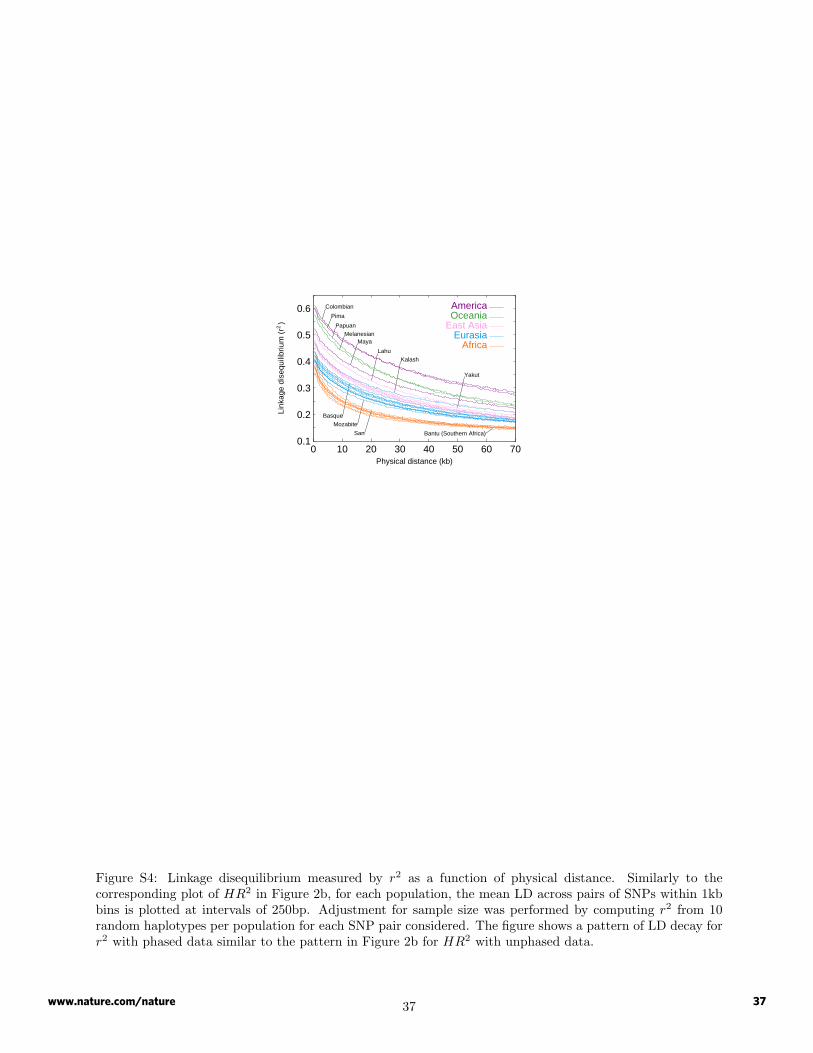
0.1
0.2
0.3
0.4
0.5
0.6
0 10 20 30 40 50 60 70
Link
age
dise
quili
briu
m (
r )
2
Physical distance (kb)
Pima
Colombian
PapuanMelanesian
Maya
LahuKalash
Yakut
Basque
Mozabite
San Bantu (Southern Africa)
AmericaOceania
East AsiaEurasia
Africa
Figure S4: Linkage disequilibrium measured by r2 as a function of physical distance. Similarly to thecorresponding plot of HR2 in Figure 2b, for each population, the mean LD across pairs of SNPs within 1kbbins is plotted at intervals of 250bp. Adjustment for sample size was performed by computing r2 from 10random haplotypes per population for each SNP pair considered. The figure shows a pattern of LD decay forr2 with phased data similar to the pattern in Figure 2b for HR2 with unphased data.
37www.nature.com/nature 37

freq
uen
cy
hap. length (kb) chromosomes
Ad
ygei
freq
uen
cy
hap. length (kb) chromosomes
Russ
ian
freq
uen
cy
hap. length (kb) chromosomes
CEU
freq
uen
cy
hap. length (kb) chromosomes
Bas
qu
e
freq
uen
cy
hap. length (kb) chromosomes
Man
den
ka
freq
uen
cy
hap. length (kb) chromosomes
YRI
freq
uen
cy
hap. length (kb) chromosomes
Yoru
ba
freq
uen
cy
hap. length (kb) chromosomes
Ban
tu(K
enya
)
freq
uen
cy
hap. length (kb) chromosomes
Ban
tu(S
. Afr
ica)
freq
uen
cy
hap. length (kb) chromosomes
Bia
kaPy
gm
y
freq
uen
cy
hap. length (kb) chromosomes
Mb
uti
Pyg
my
freq
uen
cy
hap. length (kb) chromosomes
San
freq
uen
cy
hap. length (kb) chromosomes
Moz
abit
e
freq
uen
cy
hap. length (kb) chromosomes
Bed
ou
in
freq
uen
cy
hap. length (kb) chromosomes
Pale
stin
ian
freq
uen
cy
hap. length (kb) chromosomes
Dru
ze
freq
uen
cyhap. length (kb) chromosomes
Bal
och
i
freq
uen
cy
hap. length (kb) chromosomes
Kal
ash
freq
uen
cy
hap. length (kb) chromosomes
Bu
rush
o
freq
uen
cy
hap. length (kb) chromosomes
Uyg
ur
freq
uen
cy
hap. length (kb) chromosomes
Yaku
t
freq
uen
cy
hap. length (kb) chromosomes
Dau
r
freq
uen
cy
hap. length (kb) chromosomes
Mo
ng
ola
freq
uen
cy
hap. length (kb) chromosomes
JPT
freq
uen
cy
hap. length (kb) chromosomes
CH
B
freq
uen
cy
hap. length (kb) chromosomes
Yi
freq
uen
cy
hap. length (kb) chromosomes
Lah
u
freq
uen
cy
hap. length (kb) chromosomes
Cam
bo
dia
n
freq
uen
cy
hap. length (kb) chromosomes
Co
lom
bia
n
freq
uen
cy
hap. length (kb) chromosomes
May
a
freq
uen
cy
hap. length (kb) chromosomes
Pim
a
freq
uen
cy
hap. length (kb) chromosomes
Pap
uan
freq
uen
cyhap. length (kb) chromosomes
Mel
anes
ian
0
.00000064
.0000054
.000040
.00030
.0022
.016
.12
Figure S5: Joint distribution of haplotype length and frequency. The x-axis represents haplotype frequency,indicated by number of chromosomes observed for a given haplotype in a sample of 12 chromosomes (trun-cated at one chromosome). The y-axis represents haplotype length, and the z-axis represents the density ofhaplotypes of a specific length and frequency. A heat map of the density is shown on a logarithmic scale beloweach histogram. The figure illustrates that in Africa, short low-frequency haplotypes are common, while longhigh-frequency haplotypes are almost absent. Populations from Europe, the Middle East, and Central/SouthAsia have fewer short low-frequency haplotypes and more long high-frequency haplotypes. This trend ofincreasing occurrence of long high-frequency haplotypes continues into East Asia, and finally, into Oceaniaand America.
38www.nature.com/nature 38

Ady
gei
Rus
sian
CEU
Bas
que
Man
denk
aYR
IYo
ruba
Ban
tu(K
enya
)B
antu
(S. A
fric
a)B
iaka
Pygm
yM
buti
Pygm
ySa
n
28.3 Chr. 17 28.7
Uyg
urB
urus
hoK
alas
hB
aloc
hiD
ruze
Pale
stin
ian
Bed
ouin
Moz
abite
28.3 Chr. 17 28.7
Yaku
tD
aur
Mon
gola
JPT
CH
BYi
Lahu
Cam
bodi
an Papu
anM
elan
esia
n
28.3 Chr. 17 28.7
Pim
aM
aya
Col
ombi
an
28.3 Chr. 17 28.7
0.0
0.2
0.4
0.6
0.8
28.3 28.4 28.5 28.7
Position (Mb)
Hap
loty
pe
clu
ster
ho
moz
ygo
sity
Figure S6: Haplotype cluster frequencies for a “typical” genomic region of 150 SNPs (from chromosome 17),and haplotype cluster homozygosity across the region for each population. Reduced haplotype diversity inOceania and the Americas is consistent with founder effects via migration from East Asia — in the left partof the region, it is possible that via separate founder effects the orange cluster common in East Asia rose to ahigh frequency in Oceania, while the blue-green cluster rose to a high frequency in the Americas. This figureillustrates several frequently-observed features of such plots. Africa exhibits great diversity, with commonhaplotype clusters rare or absent elsewhere. A sampling of haplotype clusters moving outward from Africatowards Oceania and the Americas is also a typical pattern. Finally, haplotypic similarity of populationsfrom the same geographic region is also evident.
39www.nature.com/nature 39

Position on chromosome 2 (Mb)
Sta
ndar
dize
d ha
plot
ype
clus
ter h
omoz
ygos
ity
−20
24
68
Position on chromosome 17 (Mb)
Sta
ndar
dize
d ha
plot
ype
clus
ter h
omoz
ygos
ity
−20
24
68
28.3 28.4 28.5 28.7135.5
A B
135.3 136.1 136.5 136.7 136.9
Figure S7: Standardized haplotype cluster homozygosity for (A) the lactase region, and (B) the “typical”genomic region of 150 SNPs shown in Figure S6. For each population, standardized homozygosity is obtainedpointwise by subtracting the mean haplotype cluster homozygosity in the population across the genomeand dividing by the standard deviation. The mean and standard deviation are obtained by using all tenhaplotype cluster datasets employed throughout our population-genetic analysis. Populations are color-coded geographically as in Figures 3 and S6. Part A shows that the CEU population has unusually highhomozygosity in the lactase region, but that homozygosities of other populations are less extreme. Part Bprovides a comparison with a typical region. The x-axis is scaled by the number of SNPs typed; correspondingphysical positions are indicated on the graphs.
40www.nature.com/nature 40

48
Mbuti Pygmy 462
48
Mbuti Pygmy 984
48
Mozabite 1263
48
Bedouin 625
48
Papuan 545
48
Russian 879
48
Yakut 962
48
Basque 1364
Bantu (Southern Africa) 993
48
0 50 100 150
Position along X chromosome (Mb)
Num
ber
of h
eter
ozyg
ous
SN
Ps
in 1
0−S
NP
win
dow
Figure S8: Identification of duplications using scans of X-chromosomal heterozygosity in males. The plotshows the number of heterozygous SNPs in sliding windows that contain 10 SNPs. Only windows of the(non-pseudoautosomal) X chromosome in which at least one SNP is heterozygous are shown, for only thenine males who had at least one window with at least three heterozygous SNPs. As duplications can lead toextended stretches of consecutive heterozygous genotypes along male X chromosomes, the high peaks arounda single position in each of the top eight plots indicate the likely presence of duplications. By contrast, theplot for Bantu (Southern Africa) 993 displays no clear peaks. The higher overall level of heterozygosity inthis individual is more likely to be due to genotyping error: individual 993 has genotyping call rate 0.9818(after reclustering), compared with values ≥ 0.9977 for each of the other eight males shown. Due to poorerdata quality, individual 993 is among the individuals not considered in the PennCNV analysis.
41www.nature.com/nature 41

Duplications at beginningof X chromosome
Position along X chromosome (Mb)
Num
ber o
f het
eroz
ygou
s SN
Ps in
10−
SNP
win
dow
45
67
89
8 9 10 11 12 13
Mbuti Pygmy 462Mbuti Pygmy 984Mozabite 1263Bedouin 625
Duplications at endof X chromosome
Position along X chromosome (Mb)
Num
ber o
f het
eroz
ygou
s SN
Ps in
10−
SNP
win
dow
45
67
89
140.2 140.3 140.4 140.5
Papuan 545Russian 879Yakut 962Basque 1364
Figure S9: Identification of duplications in males on two parts of the X chromosome. The plot shows thenumber of heterozygous SNPs in sliding windows that contain 10 SNPs, magnified near two X-chromosomalregions in which duplications were detected. Papuan individual 545 was not included in the PennCNV analysis,and consequently, the duplication in this individual was not detectable by PennCNV. All other duplicationsdetected by extended stretches of X-chromosomal heterozygosity in males were also detected by PennCNV.
42www.nature.com/nature 42

A
0
0.001
0.002
0.003
0.004
0.005
0.006
0.007
0 0.01 0.02 0.03 0.04 0.05
Est
imat
ed fa
lse
posi
tive
rate
True mean frequencyof copy number variants at 396 CNV loci
B
0
0.1
0.2
0.3
0.4
0.5
0.6
0.7
0 0.01 0.02 0.03 0.04 0.05
Est
imat
ed fa
lse
nega
tive
rate
True mean frequencyof copy number variants at 396 CNV loci
Figure S10: Estimated false positive and false negative rates as functions of the unknown true mean frequencyof copy-number variants across 396 CNV loci. The plots are based on equations 3 and 4, with an estimatedconcordance of duplicates equal to 871/980 ≈ 0.89, the average concordance across duplicate pairs. (A)False positive rate. (B) False negative rate. The figure shows a low false positive rate for CNV calls and acomparatively higher false negative rate.
43www.nature.com/nature 43

A
0
0.001
0.002
0.003
0.004
0.005
0.006
0.007
0 0.01 0.02 0.03 0.04 0.05
Est
imat
ed fa
lse
posi
tive
rate
True mean frequencyof copy number variants at 396 CNV loci
B
0
0.1
0.2
0.3
0.4
0.5
0.6
0.7
0 0.01 0.02 0.03 0.04 0.05
Est
imat
ed fa
lse
nega
tive
rate
True mean frequencyof copy number variants at 396 CNV loci
Figure S11: Estimated false positive and false negative rates as functions of the unknown true mean frequencyof copy-number variants across 396 CNV loci. The plots are based on equations 3 and 4, with an estimatedconcordance of duplicates equal to 51/67 ≈ 0.76, a value estimated by pooling duplicate pairs. (A) Falsepositive rate. (B) False negative rate. The figure shows a low false positive rate for CNV calls and acomparatively higher false negative rate.
44www.nature.com/nature 44

0 0.02 0.04 0.06 0.08 0.1 0.12 0.14 0.160
20
40
60
80
100
120
140
160
180
200
Num
ber o
f CN
V lo
ci
Allele frequency
Figure S12: Allele frequency spectrum for the copy-number variants at 1302 autosomal CNV loci in 405unrelated individuals from 29 populations. The 1/810 frequency class is not plotted and contains 906 loci.The figure illustrates that most CNVs were observed to be rare.
45www.nature.com/nature 45

0 0.2 0.4 0.60
50
100
150
Allele frequencyN
umbe
r of C
NV
loci
AFRICA
0 0.2 0.4 0.60
50
100
150
Allele frequency
Num
ber o
f CN
V lo
ciAMERICA
0 0.2 0.4 0.60
50
100
150
Allele frequency
Num
ber o
f CN
V lo
ci
CENTRAL/SOUTH ASIA
0 0.2 0.4 0.60
50
100
150
Allele frequency
Num
ber o
f CN
V lo
ci
EAST ASIA
0 0.2 0.4 0.60
50
100
150
Allele frequency
Num
ber o
f CN
V lo
ci
EUROPE
0 0.2 0.4 0.60
50
100
150
Allele frequency
Num
ber o
f CN
V lo
ci
MIDDLE EAST
0 0.2 0.4 0.60
50
100
150
Allele frequency
Num
ber o
f CN
V lo
ci
OCEANIA
Figure S13: Allele frequency spectra for the copy-number variants at 1302 autosomal CNV loci, consideringunrelated individuals in 7 geographic regions. To adjust for sample size differences among regions, we useda resampling procedure. The alleles of each individual were partitioned into two “pseudo-genomes,” eachcontaining one allele at each CNV locus. Next, for each CNV locus, 38 haploid pseudo-genomes were randomlydrawn (without replacement) from each geographic region and the frequency of each CNV was calculated.An average frequency for each CNV was then computed across 1000 sets of pseudo-genomes (with the setsindependently chosen for different CNV loci). Using this average frequency, loci were classified into one of39 allele frequency bins: [0, 1/38], (1/38, 2/38], ..., (36/38, 37/38], (37/38, 1]. After averaging, the numbersof CNV loci in the [0, 1/38] bin were as follows: Africa — 1281, Middle East — 1285, Europe — 1266,Central/South Asia — 1259, East Asia — 1288, Oceania — 1086, and America — 1270.
46www.nature.com/nature 46

AdygeiBalochiBantu (Kenya)Bantu (S. Africa)BasqueBedouinBiaka PygmyBurusho
CambodianColombianDaurDruzeKalashLahuMandenkaMaya
Mbuti PygmyMelanesianMongolaMozabitePalestinianPapuanPimaRussian
SanUygurYakutYiYoruba
Africa
EuropeMiddle East
C/S AsiaEast AsiaOceaniaAmerica
Figure S14: Multidimensional scaling representation of the genetic distance matrix for the CNV dataset.Three outliers removed from the matrix for the CNV plot in Figure 1d (Kalash, Melanesian, and Papuan)are retained in the analysis that underlies this plot. The geographic clustering visible in Figure 1d is lessvisible in this plot, with the outliers included.
47www.nature.com/nature 47

K=2
K=3
K=4
K=5
K=6
K=7
K=8
San
Mb
uti
Pyg
my
Bia
ka P
ygm
y
Ban
tu (
Ken
ya)
Ban
tu (
S. A
fric
a)Y
oru
ba
Man
den
ka
Mo
zab
ite
Bed
ou
in
Pal
esti
nia
n
Dru
ze
Bas
qu
eR
uss
ian
Ad
ygei
Bal
och
iK
alas
hB
uru
sho
Uyg
ur
Yak
ut
Mo
ng
ola
Dau
r Yi
Cam
bo
dia
nL
ahu
Mel
anes
ian
Pap
uan
Pim
aM
aya
Co
lom
bia
n
Figure S15: Population structure inferred from SNP sets of the same size and frequency spectrum as theCNV dataset, for various choices of the number of clusters, K. The figure shows that the level of “noise” inpopulation structure plots based on the reduced SNP datasets is comparable to the corresponding level inplots based on the CNV dataset (Figures 1c and S24).
48www.nature.com/nature 48

A B
AdygeiBalochiBantu (Kenya)Bantu (S. Africa)BasqueBedouinBiaka PygmyBurusho
CambodianColombianDaurDruzeKalashLahuMandenkaMaya
Mbuti PygmyMelanesianMongolaMozabitePalestinianPapuanPimaRussian
SanUygurYakutYiYoruba
Africa
EuropeMiddle East
C/S AsiaEast AsiaOceaniaAmerica
Figure S16: Multidimensional scaling representations of genetic distance matrices for individual geographicregions, based on a reduced SNP dataset of the same size and frequency spectrum as the CNV dataset. (A)All populations. (B) Two outliers removed (Basque and Russian). The figure shows that the level of “noise”in multidimensional scaling plots based on the SNP dataset is comparable to the corresponding level in plotsbased on the CNV dataset (Figures 1d and S14).
49www.nature.com/nature 49

QU
ALI
TY C
ON
TRO
LG
ENO
TYPI
NG
individuals with <95% call rate
495 individuals
18,667 SNPs/individual
SNPs with call rate <98%
comparison with 122 SNPs of Conrad et al. (2006)
SNPs that were not on both chip versions(v1 & v3) 10,286 SNPs/version1 only
16,400 SNPs/version3 only
known duplicates
known labeling errors in the HGDP-CEPH cell repository
2 discordant individuals
7 individuals
513 individuals from 29 populations
Reclustering of genotypes in Beadstudio 3.1.4, discarding all genotypes below no-call threshold 0.15
495 individuals
545,066 SNPs/individual
further qualitychecks on SNPs
489 SNPs/individual
1 individual
495 individuals
526,399 SNPs/individual
485 individuals
526,399 SNPs/individual
525,910 SNPs/individual
485 individuals
18 individuals
197 individuals genotyped on HumanHap550 v3
316 individuals genotyped on HumanHap550 v1
Figure S17: Flow chart of the genotyping and quality control process for SNP genotypes.
50www.nature.com/nature 50

0
0.1
0.2
0.3
0.4
0.5
0.6
0.7
0.8
0.9
1
0 50 100 150 200 250 300
Bantu (Kenya)
Bantu (S.Africa)
Bedouin
Biaka Pygmy
Druze
Kalash
Mandenka
Mbuti Pygmy
Melanesian
Mozabite
Papuan
Palestinian
San
Yoruba
call rate
50% GC
10% GC
minor allele frequency
B/B frequency
A/A frequency
A/B frequency
sample number
Figure S18: Quality control plot for 303 individuals genotyped on HumanHap550 version 1 BeadChips. The303 individuals plotted are those with a genotype call rate >95% after genotype reclustering. Each backgroundcolor represents the individuals from a single population, and within each population, individuals are sortedby HGDP-CEPH identification number. Black diamonds indicate call rates, blue diamonds indicate the 50%GC score (median GenCall score across SNPs), red diamonds indicate the 10% GC score (tenth percentile ofthe ranked GenCall scores), green diamonds indicate the minor allele frequency, turquoise diamonds indicatethe frequency of B/B calls, gray diamonds indicate the frequency of A/A calls, and orange diamonds indicatethe frequency of A/B calls. For a given individual and SNP, the GenCall score is a measure of data qualitythat takes into account the fit of the individual genotype to defined genotype clusters. Scores above 0.7indicate high-quality genotypes and scores below 0.2 indicate low-quality genotypes. We used a GenCallthreshold of 0.15 in measuring the call rate.
51www.nature.com/nature 51

0
0.1
0.2
0.3
0.4
0.5
0.6
0.7
0.8
0.9
1
0 20 40 60 80 100 120 140 160 180
sample number
Adygei
Balochi
Basque
Bedouin
Burusho
Cambodian
Colombian
Daur
Druze
Kalash
Lahu
Maya
Melanesian
Mongola
Papuan
Pima
Russian
Uygur
Yakut
Yi
call rate
50% GC
10% GC
minor allele frequency
B/B frequency
A/A frequency
A/B frequency
Figure S19: Quality control plot for 192 individuals genotyped on HumanHap550 version 3 BeadChips. The192 individuals plotted are those with a genotype call rate >95% after genotype reclustering. Each backgroundcolor represents the individuals from a single population, and within each population, individuals are sortedby HGDP-CEPH identification number. Black diamonds indicate call rates, blue diamonds indicate the 50%GC score (median GenCall score across SNPs), red diamonds indicate the 10% GC score (tenth percentile ofthe ranked GenCall scores), green diamonds indicate the minor allele frequency, turquoise diamonds indicatethe frequency of B/B calls, gray diamonds indicate the frequency of A/A calls, and orange diamonds indicatethe frequency of A/B calls. For a given individual and SNP, the GenCall score is a measure of data qualitythat takes into account the fit of the individual genotype to defined genotype clusters. Scores above 0.7indicate high-quality genotypes and scores below 0.2 indicate low-quality genotypes. We used a GenCallthreshold of 0.15 in measuring the call rate. In the quality control plots, the minor allele at a locus is definedwith respect to the BeadStudio project, and may differ between version 1 and version 3 BeadStudio projects.
52www.nature.com/nature 52
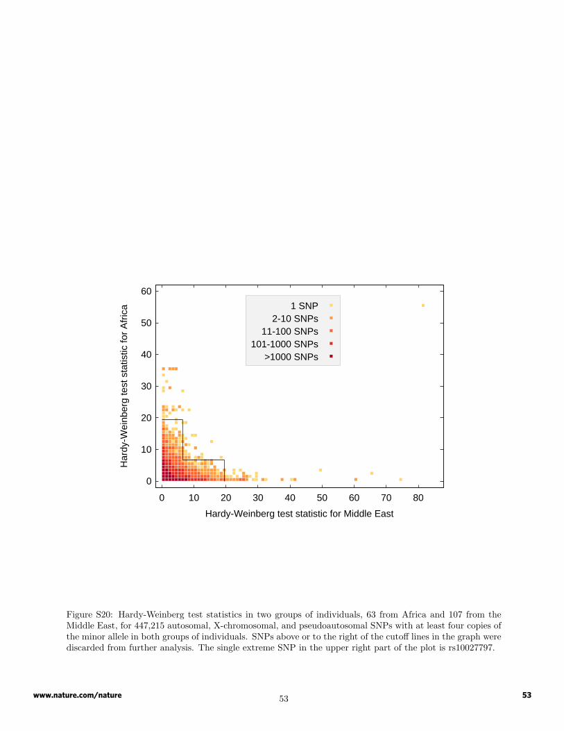
0
10
20
30
40
50
60
0 10 20 30 40 50 60 70 80
Har
dy-W
einb
erg
test
sta
tistic
for
Afr
ica
Hardy-Weinberg test statistic for Middle East
1 SNP2-10 SNPs
11-100 SNPs101-1000 SNPs
>1000 SNPs
Figure S20: Hardy-Weinberg test statistics in two groups of individuals, 63 from Africa and 107 from theMiddle East, for 447,215 autosomal, X-chromosomal, and pseudoautosomal SNPs with at least four copies ofthe minor allele in both groups of individuals. SNPs above or to the right of the cutoff lines in the graph werediscarded from further analysis. The single extreme SNP in the upper right part of the plot is rs10027797.
53www.nature.com/nature 53
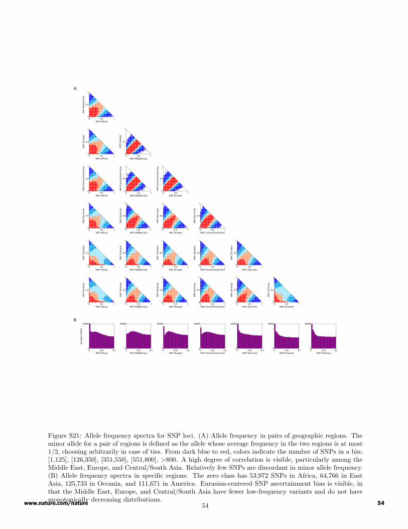
A
0
0.5
1
0 0.5 1
MA
F (E
urop
e)
MAF (Africa)
0
0.5
1
0 0.5 1
MA
F (M
iddl
e Ea
st)
MAF (Africa)
0
0.5
1
0 0.5 1
MA
F (C
entr
al/S
outh
Asi
a)
MAF (Africa)
0
0.5
1
0 0.5 1
MA
F (E
ast A
sia)
MAF (Africa)
0
0.5
1
0 0.5 1
MA
F (O
cean
ia)
MAF (Africa)
0
0.5
1
0 0.5 1
MA
F (A
mer
ica)
MAF (Africa)
MAF (Middle East)
MA
F (E
urop
e)
0
0.5
1
0 0.5 1
MA
F (C
entr
al/S
outh
Asi
a)
MAF (Europe)
0
0.5
1
0 0.5 1
MA
F (E
ast A
sia)
MAF (Europe)
0
0.5
1
0 0.5 1
MA
F (O
cean
ia)
MAF (Europe)
0
0.5
1
0 0.5 1
MA
F (A
mer
ica)
MAF (Europe)
0
0.5
1
0 0.5 1
MA
F (C
entr
al/S
outh
Asi
a)
MAF (Middle East)
0
0.5
1
0 0.5 1
MA
F (E
ast A
sia)
MAF (Middle East)
0
0.5
1
0 0.5 1
MA
F (O
cean
ia)
MAF (Middle East)
0
0.5
1
0 0.5 1
MA
F (A
mer
ica)
MAF (Middle East)
0
0.5
1
0 0.5 1
MA
F (E
ast A
sia)
MAF (Central/South Asia)
0
0.5
1
0 0.5 1
MA
F (O
cean
ia)
MAF (Central/South Asia)
0
0.5
1
0 0.5 1
MA
F (A
mer
ica)
MAF (Central/South Asia)
0
0.5
1
0 0.5 1
MA
F (O
cean
ia)
MAF (East Asia)
0
0.5
1
0 0.5 1
MA
F (A
mer
ica)
MAF (East Asia)
0
0.5
1
0 0.5 1
MA
F (A
mer
ica)
MAF (Oceania)
B
0
50000
0 0.25 0.5
Num
ber o
f SN
Ps
MAF (Africa)
0
50000
0 0.25 0.5MAF (Europe)
0
50000
0 0.25 0.5MAF (Middle East)
0
50000
0 0.25 0.5MAF (Central/South Asia)
0
50000
0 0.25 0.5MAF (East Asia)
0
50000
0 0.25 0.5MAF (Oceania)
0
50000
0 0.25 0.5MAF (America)
0
0.5
1
0 0.5 1
Figure S21: Allele frequency spectra for SNP loci. (A) Allele frequency in pairs of geographic regions. Theminor allele for a pair of regions is defined as the allele whose average frequency in the two regions is at most1/2, choosing arbitrarily in case of ties. From dark blue to red, colors indicate the number of SNPs in a bin:[1,125], [126,350], [351,550], [551,800], >800. A high degree of correlation is visible, particularly among theMiddle East, Europe, and Central/South Asia. Relatively few SNPs are discordant in minor allele frequency.(B) Allele frequency spectra in specific regions. The zero class has 53,972 SNPs in Africa, 64,766 in EastAsia, 125,733 in Oceania, and 111,671 in America. Eurasian-centered SNP ascertainment bias is visible, inthat the Middle East, Europe, and Central/South Asia have fewer low-frequency variants and do not havemonotonically decreasing distributions.
54www.nature.com/nature 54

0 200 400 600 800 10000
100
200
300
400
500
600
700
Length (kb)
Num
ber o
f CN
Vs
0 200 400 600 800 10000
40
80
120
160
200
Length (kb)
Num
ber o
f dup
licat
ions
0 200 400 600 800 10000
100
200
300
400
500
Length (kb)
Num
ber o
f del
etio
ns
A
B
C
Figure S22: Distribution of the lengths of 3503 autosomal CNVs. (A) All CNVs. (B) Duplications (1117).(C) Deletions (2386). In kilobases, the bins in each histogram are (0, 20], ... , (980, 1000].
55www.nature.com/nature 55

0.1
0.2
0.3
0.4
0.5
0.6
0.1 0.2 0.3 0.4 0.5 0.6
Link
age
dise
quili
briu
m (
r )
2
Linkage disequilibrium (HR ) 2
AmericaOceania
East AsiaEurasia
Africa
Figure S23: Comparison of LD measured by r2 on phased data to LD measured by HR2 on unphased data.For each population, ordered pairs (HR2, r2) are obtained at 250bp intervals and are connected in increasingorder of physical distance. The figure illustrates a close relationship between HR2 computed on unphaseddata and r2 computed on phased data.
56www.nature.com/nature 56

SNPs
K=2
K=3
K=4
K=5
K=6
K=7
K=8
K=9
K=1
0
San
Mb
uti
Pyg
my
Bia
ka P
ygm
y
Ban
tu (
Ken
ya)
Ban
tu (
S. A
fric
a)Y
oru
ba
Man
den
ka
Mo
zab
ite
Bed
ou
in
Pal
esti
nia
n
Dru
ze
Bas
qu
eR
uss
ian
Ad
ygei
Bal
och
iK
alas
hB
uru
sho
Uyg
ur
Yak
ut
Mo
ng
ola
Dau
r Yi
Cam
bo
dia
nL
ahu
Mel
anes
ian
Pap
uan
Pim
aM
aya
Co
lom
bia
n
Haplotypes
San
Mb
uti
Pyg
my
Bia
ka P
ygm
y
Ban
tu (
Ken
ya)
Ban
tu (
S. A
fric
a)Y
oru
ba
Man
den
ka
Mo
zab
ite
Bed
ou
in
Pal
esti
nia
n
Dru
ze
Bas
qu
eR
uss
ian
Ad
ygei
Bal
och
iK
alas
hB
uru
sho
Uyg
ur
Yak
ut
Mo
ng
ola
Dau
r Yi
Cam
bo
dia
nL
ahu
Mel
anes
ian
Pap
uan
Pim
aM
aya
Co
lom
bia
n
CNVs
San
Mb
uti
Pyg
my
Bia
ka P
ygm
y
Ban
tu (
Ken
ya)
Ban
tu (
S. A
fric
a)Y
oru
ba
Man
den
ka
Mo
zab
ite
Bed
ou
in
Pal
esti
nia
n
Dru
ze
Bas
qu
eR
uss
ian
Ad
ygei
Bal
och
iK
alas
hB
uru
sho
Uyg
ur
Yak
ut
Mo
ng
ola
Dau
r Yi
Cam
bo
dia
nL
ahu
Mel
anes
ian
Pap
uan
Pim
aM
aya
Co
lom
bia
n
Figure S24: Population structure inferred from SNPs, haplotypes, and CNVs for various choices of the numberof clusters, K. The plots with K ≤ 6 are copied in Figure 1c. The Bedouin and two Mozabites with highestimated membership in the cluster corresponding to Africans in SNP and haplotype analyses are the sameindividuals seen to lie on the path connecting Africans to the remaining individuals from the Middle Eastin the multidimensional scaling analysis (Figure 1d). Two populations with a considerable degree of mixedmembership between the clusters corresponding to Eurasia and East Asia — Burusho and Uygur — are alsothe two populations most intermediate in the MDS analysis between Europe and East Asia.
57www.nature.com/nature 57

2 4 6 8 10
−35
0000
00−
2500
0000
−15
0000
00−
5000
000
SNPs
Number of clusters (K)
Log
likel
ihoo
d
2 3 4 5 6 7 8 9 10 2 4 6 8 10
−25
0000
0−
2300
000
−21
0000
0
SNPs
Number of clusters (K)
Log
likel
ihoo
d
2 3 4 5 6 7 8 9 10
2 4 6 8 10
−10
0000
000
−60
0000
00−
2000
0000
Haplotypes
Number of clusters (K)
Log
likel
ihoo
d
2 3 4 5 6 7 8 9 10 2 4 6 8 10−11
0000
00−
1060
0000
−10
2000
00
Haplotypes
Number of clusters (K)
Log
likel
ihoo
d
2 3 4 5 6 7 8 9 10
2 4 6 8 10
−22
000
−18
000
−14
000
−10
000
CNVs
Number of clusters (K)
Log
likel
ihoo
d
2 3 4 5 6 7 8 9 10 2 4 6 8 10
−14
000
−13
000
−12
000
−11
000
−10
000
CNVs
Number of clusters (K)
Log
likel
ihoo
d
2 3 4 5 6 7 8 9 10
Figure S25: Log likelihood as a function of the number of clusters, based on Structure runs applied to thefull worldwide dataset. Likelihoods for all 40 replicates at a given K are shown. The plots on the right sideare magnified versions of the plots on the left.
58www.nature.com/nature 58

2 4 6 8 10
−28
0000
0−
2400
000
SNPs
Number of clusters (K)
Log
likel
ihoo
d
2 3 4 5 6 7 8 9 10 2 4 6 8 10
−25
0000
0−
2300
000
−21
0000
0
SNPs
Number of clusters (K)
Log
likel
ihoo
d
2 3 4 5 6 7 8 9 10
2 4 6 8 10−20
0000
00−
1600
0000
−12
0000
00
Haplotypes
Number of clusters (K)
Log
likel
ihoo
d
2 3 4 5 6 7 8 9 10 2 4 6 8 10−11
0000
00−
1060
0000
−10
2000
00
Haplotypes
Number of clusters (K)
Log
likel
ihoo
d
2 3 4 5 6 7 8 9 10
2 4 6 8 10
−13
000
−12
000
−11
000
−10
000
CNVs
Number of clusters (K)
Log
likel
ihoo
d
2 3 4 5 6 7 8 9 10 2 4 6 8 10
−14
000
−13
000
−12
000
−11
000
−10
000
CNVs
Number of clusters (K)
Log
likel
ihoo
d
2 3 4 5 6 7 8 9 10
Figure S26: Log likelihood as a function of the number of clusters, based on Structure runs applied to thefull worldwide dataset. Likelihoods are shown only for Structure runs in the most frequent mode. The plotson the right side are magnified versions of the plots on the left.
59www.nature.com/nature 59

2 3 4 5 6 7 8−35
0000
0−
5000
00
africa[, 1]
Log
likel
ihoo
d
2 3 4 5 6 7 8Number of clusters (K)
Africa
2 3 4 5 6 7 8
−48
0000
−54
0000
africa[, 1]
Log
likel
ihoo
d
2 3 4 5 6 7 8Number of clusters (K)
Africa
2 3 4 5
−80
0000
−85
0000
me[, 1]
Log
likel
ihoo
d
Number of clusters (K)
Middle East
2 3 4 5
−74
0000
me[, 1]
Log
likel
ihoo
d
Number of clusters (K)
Middle East
−68
0000
2 3 4 5−27
0000
−21
0000
europe[, 1]
Log
likel
ihoo
d
Number of clusters (K)
Europe
2 3 4 5−21
0000
−20
0000
europe[, 1]
Log
likel
ihoo
d
Number of clusters (K)
Europe
2 3 4 5−55
0000
−25
0000
cs[, 1]
Log
likel
ihoo
d
Number of clusters (K)
C/S Asia
2 3 4 5−26
0000
−23
5000
cs[, 1]
Log
likel
ihoo
d
Number of clusters (K)
C/S Asia
2 3 4 5 6 7 8−55
0000
−30
0000
eastasia[, 1]
Log
likel
ihoo
d
Number of clusters (K)
East Asia
2 3 4 5 6 7 8−32
0000
−28
0000
eastasia[, 1]
Log
likel
ihoo
d
Number of clusters (K)
East Asia
2 3 4 5−16
0000
−11
0000
oceania[, 1]
Log
likel
ihoo
d
Number of clusters (K)
Oceania
2 3 4 5−11
0000
−10
4000
oceania[, 1]
Log
likel
ihoo
d
Number of clusters (K)
Oceania
2 3 4 5
−40
0000
−10
0000
america[, 1]
Log
likel
ihoo
d
Number of clusters (K)
America
2 3 4 5−12
0000
−10
0000
america[, 1]
Log
likel
ihoo
d
Number of clusters (K)
America
Figure S27: Log likelihood as a function of the number of clusters, based on Structure runs applied toindividual geographic regions. Likelihoods for all 40 replicates at a given K are shown. The plots on theright side are magnified versions of the plots on the left.
60www.nature.com/nature 60

2 3 4 5 6 7 8−
5000
00−
2000
000
africa[, 1]
Log
likel
ihoo
d
2 3 4 5 6 7 8Number of clusters (K)
Africa
2 3 4 5 6 7 8
−50
0000
−20
0000
0
africa[, 1]
Log
likel
ihoo
d
2 3 4 5 6 7 8Number of clusters (K)
Africa
2 3 4 5−68
9000
−68
3000
me[, 1]
Log
likel
ihoo
d
Number of clusters (K)
Middle East
2 3 4 5
−74
0000
me[, 1]
Log
likel
ihoo
d
Number of clusters (K)
Middle East
−68
0000
2 3 4 5
−20
3000
−20
0500
europe[, 1]
Log
likel
ihoo
d
Number of clusters (K)
Europe
2 3 4 5−21
0000
−20
0000
europe[, 1]
Log
likel
ihoo
d
Number of clusters (K)
Europe
2 3 4 5−29
0000
−24
0000
cs[, 1]
Log
likel
ihoo
d
Number of clusters (K)
C/S Asia
2 3 4 5−26
0000
−23
5000
cs[, 1]
Log
likel
ihoo
d
Number of clusters (K)
C/S Asia
2 3 4 5 6 7 8−38
0000
−30
0000
eastasia[, 1]
Log
likel
ihoo
d
Number of clusters (K)
East Asia
2 3 4 5 6 7 8−32
0000
−28
0000
eastasia[, 1]
Log
likel
ihoo
d
Number of clusters (K)
East Asia
2 3 4 5
−11
0000
−15
0000
oceania[, 1]
Log
likel
ihoo
d
Number of clusters (K)
Oceania
2 3 4 5−11
0000
−10
4000
oceania[, 1]
Log
likel
ihoo
d
Number of clusters (K)
Oceania
2 3 4 5
−40
0000
−10
0000
america[, 1]
Log
likel
ihoo
d
Number of clusters (K)
America
2 3 4 5−25
0000
−10
0000
america[, 1]
Log
likel
ihoo
d
Number of clusters (K)
America
Figure S28: Log likelihood as a function of the number of clusters, based on Structure runs applied toindividual geographic regions. Likelihoods are shown only for Structure runs in the most frequent mode.The plots on the right side are magnified versions of the plots on the left. For Europe with K = 5, there wasno mode, and the point plotted corresponds to the single highest-likelihood run.
61www.nature.com/nature 61

0 10,000 20,000 30,0000
0.1
0.2
0.3
0.4
Geographic distance (km)
Pairw
ise
F ST g
enet
ic d
ista
nce
0 10,000 20,000 30,0000
0.1
0.2
0.3
Geographic distance (km)0 10,000 20,000 30,000
Geographic distance (km)
0
0.1
0.2
Pairwise F
ST genetic distance
AfricaEurasiaEast AsiaOceaniaAmerica
A B C
Figure S29: FST between pairs of populations, plotted as a function of geographic distance between thepopulations. Only population pairs that contain at least one African population are shown. (A) SNPs.The Pearson correlation between FST and geographic distance is 0.74 and the regression line is FST =(9.057 × 10⁻⁶)D + 0.045, where D represents distance in kilometers. R2 = 0.54. (B) Haplotypes. ThePearson correlation is 0.74, the regression line is FST = (6.220× 10⁻⁶)D + 0.029, and R2 = 0.54. (C) CNVs.The Pearson correlation is 0.49, the regression line is FST = (2.494 × 10⁻⁶)D + 0.023, and R2 = 0.24. Theplots indicate a reasonably close relationship between genetic distance and geographic distance for SNPs andhaplotypes, and a weaker relationships for CNVs. The SNP plot is copied in Figure 2a.
62www.nature.com/nature 62

0 0.02 0.04 0.06 0.08 0.1 0.12 0.14 0.160
20
40
60
80
100
120
140
160
180
200
Num
ber o
f SN
Ps
Allele frequency
Figure S30: Allele frequency spectrum for each of five sets of 396 non-singleton SNPs in 405 unrelated indi-viduals from 29 populations. The frequency spectrum is matched as closely as possible to the correspondingfrequency spectrum of CNV loci in Figure S12.
63www.nature.com/nature 63

References
1. Cann, H. M., de Toma, C., Cazes, L., Legrand, M.-F., Morel, V., Piouffre, L., Bodmer, J., Bodmer, W. F.,Bonne-Tamir, B., Cambon-Thomsen, A., Chen, Z., Chu, J., Carcassi, C., Contu, L., Du, R., Excoffier,L., Ferrara, G. B., Friedlaender, J. S., Groot, H., Gurwitz, D., Jenkins, T., Herrera, R. J., Huang, X.,Kidd, J., Kidd, K. K., Langaney, A., Lin, A. A., Mehdi, S. Q., Parham, P., Piazza, A., Pistillo, M. P.,Qian, Y., Shu, Q., Xu, J., Zhu, S., Weber, J. L., Greely, H. T., Feldman, M. W., Thomas, G., Dausset,J., and Cavalli-Sforza, L. L. A human genome diversity cell line panel. Science 296, 261–262 (2002).
2. Cavalli-Sforza, L. L. The Human Genome Diversity Project: past, present and future. Nature Rev. Genet.6, 333–340 (2005).
3. The International HapMap Consortium. A haplotype map of the human genome. Nature 437, 1299–1320(2005).
4. Simon-Sanchez, J., Scholz, S., Fung, H.-C., Matarin, M., Hernandez, D., Gibbs, J. R., Britton, A.,Wavrant de Vrieze, F., Peckham, E., Gwinn-Hardy, K., Crawley, A., Keen, J. C., Nash, J., Borgaonkar,D., Hardy, J., and Singleton, A. Genome-wide SNP assay reveals structural genomic variation, extendedhomozygosity and cell-line induced alterations in normal individuals. Hum. Mol. Genet. 16, 1–14 (2007).
5. Conrad, D. F., Jakobsson, M., Coop, G., Wen, X., Wall, J. D., Rosenberg, N. A., and Pritchard, J. K. Aworldwide survey of haplotype variation and linkage disequilibrium in the human genome. Nature Genet.38, 1251–1260 (2006).
6. Rosenberg, N. A. Standardized subsets of the HGDP-CEPH Human Genome Diversity Cell Line Panel,accounting for atypical and duplicated samples and pairs of close relatives. Ann. Hum. Genet. 70, 841–847(2006).
7. Rosenberg, N. A., Pritchard, J. K., Weber, J. L., Cann, H. M., Kidd, K. K., Zhivotovsky, L. A., andFeldman, M. W. Genetic structure of human populations. Science 298, 2381–2385 (2002).
8. Rosenberg, N. A., Mahajan, S., Ramachandran, S., Zhao, C., Pritchard, J. K., and Feldman, M. W.Clines, clusters, and the effect of study design on the inference of human population structure. PLoSGenet. 1, 660–671 (2005).
9. Weir, B. S. Genetic Data Analysis II. Sinauer, Sunderland, MA (1996).
10. Sabatti, C. and Risch, N. Homozygosity and linkage disequilibrium. Genetics 160, 1707–1719 (2002).
11. Rosenberg, N. A. and Blum, M. G. B. Sampling properties of homozygosity-based statistics for linkagedisequilibrium. Math. Biosci. 208, 33–47 (2007).
12. Ramachandran, S., Deshpande, O., Roseman, C. C., Rosenberg, N. A., Feldman, M. W., and Cavalli-Sforza, L. L. Support from the relationship of genetic and geographic distance in human populations fora serial founder effect originating in Africa. Proc. Natl. Acad. Sci. USA 102, 15942–15947 (2005).
13. Szpiech, Z. A., Jakobsson, M., and Rosenberg, N. A. ADZE: Allelic Diversity Analyzer version 1.0.http://rosenberglab.bioinformatics.med.umich.edu/adze.html, (2007).
14. Kalinowski, S. T. Counting alleles with rarefaction: private alleles and hierarchical sampling designs.Conserv. Genet. 5, 539–543 (2004).
15. Pritchard, J. K., Stephens, M., and Donnelly, P. Inference of population structure using multilocusgenotype data. Genetics 155, 945–959 (2000).
16. Falush, D., Stephens, M., and Pritchard, J. K. Inference of population structure using multilocus genotypedata: linked loci and correlated allele frequencies. Genetics 164, 1567–1587 (2003).
17. Rosenberg, N. A. DISTRUCT: a program for the graphical display of population structure. Mol. Ecol.Notes 4, 137–138 (2004).
18. Jakobsson, M. and Rosenberg, N. A. CLUMPP: a cluster matching and permutation program for dealingwith label switching and multimodality in analysis of population structure. Bioinformatics 23, 1801–1806(2007).
64www.nature.com/nature 64

19. Wang, S., Lewis Jr., C. M., Jakobsson, M., Ramachandran, S., Ray, N., Bedoya, G., Rojas, W., Parra,M. V., Molina, J. A., Gallo, C., Mazzotti, G., Poletti, G., Hill, K., Hurtado, A. M., Labuda, D., Klitz,W., Barrantes, R., Bortolini, M. C., Salzano, F. M., Petzl-Erler, M. L., Tsuneto, L. T., Llop, E., Roth-hammer, F., Excoffier, L., Feldman, M. W., Rosenberg, N. A., and Ruiz-Linares, A. Genetic variationand population structure in Native Americans. PLoS Genet. 3, 2049–2067 (2007).
20. Saitou, N. and Nei, M. The neighbor-joining method: a new method for reconstructing phylogenetictrees. Mol. Biol. Evol. 4, 406–425 (1987).
21. Minch, E., Ruiz Linares, A., Goldstein, D. B., Feldman, M. W., and Cavalli-Sforza, L. L. MICROSAT(version 2.alpha): a program for calculating statistics on microsatellite data. Department of Genetics,Stanford University, Stanford, CA (1998).
22. Felsenstein, J. PHYLIP (Phylogeny Inference Package) version 3.65. Department of Genome Sciences,University of Washington, Seattle (2005).
23. Bryant, D. A classification of consensus methods for phylogenetics. In BioConsensus, Janowitz, M. F., La-pointe, F.-J., McMorris, F. R., Mirkin, B., and Roberts, F. S., editors, 163–183. American MathematicalSociety, Providence (2003).
24. Mardia, K. V., Kent, J. T., and Bibby, J. M. Multivariate Analysis. Academic Press, London (1979).
25. Everitt, B. S. and Hothorn, T. A Handbook of Statistical Analyses Using R. Chapman & Hall/CRC,Boca Raton (2006).
26. Scheet, P. and Stephens, M. A fast and flexible statistical model for large-scale population genotypedata: applications to inferring missing genotypes and haplotypic phase. Am. J. Hum. Genet. 78, 629–644 (2006).
27. Hudson, R. R. Linkage disequilibrium and recombination. In Handbook of Statistical Genetics, Balding,D. J., Bishop, M., and Cannings, C., editors, chapter 11, 309–324. Wiley, Chichester, UK (2001).
28. Wang, K., Li, M., Hadley, D., Liu, R., Glessner, J., Grant, S. F. A., Hakonarson, H., and Bucan,M. PennCNV: an integrated hidden Markov model designed for high-resolution copy number variationdetection in whole-genome SNP genotyping data. Genome Res. 17, 1665–1674 (2007).
29. Walter, S. D. and Irwig, L. M. Estimation of test error rates, disease prevalence and relative risk frommisclassified data: a review. J. Clin. Epidemiol. 41, 923–937 (1988).
30. Hui, S. L. and Zhou, X. H. Evaluation of diagnostic tests without gold standards. Stat. Methods Med.Res. 7, 354–370 (1998).
31. Enøe, C., Georgiadis, M. P., and Johnson, W. O. Estimation of sensitivity and specificity of diagnostictests and disease prevalence when the true disease state is unknown. Prev. Vet. Med. 45, 61–81 (2000).
32. Pepe, M. S. The Statistical Evaluation of Medical Tests for Classification and Prediction. Oxford Uni-versity Press, Oxford (2003).
33. Jakobsdottir, J. and Weeks, D. E. Estimating prevalence, false-positive rate, and false-negative rate withuse of repeated testing when true responses are unknown. Am. J. Hum. Genet. 81, 1111–1113 (2007).
34. Lynch, A. G., Marioni, J. C., and Tavare, S. Numbers of copy-number variations and false-negative rateswill be underestimated if we do not account for the dependence between repeated experiments. Am. J.Hum. Genet. 81, 418–420 (2007).
35. Wong, K. K., deLeeuw, R. J., Dosanjh, N. S., Kimm, L. R., Cheng, Z., Horsman, D. E., MacAulay,C., Ng, R. T., Brown, C. J., Eichler, E. E., and Lam, W. L. A comprehensive analysis of commoncopy-number variations in the human genome. Am. J. Hum. Genet. 80, 91–104 (2007).
36. Sharp, A. J., Locke, D. P., McGrath, S. D., Cheng, Z., Bailey, J. A., Vallente, R. U., Pertz, L. M.,Clark, R. A., Schwartz, S., Segraves, R., Oseroff, V. V., Albertson, D. G., Pinkel, D., and Eichler, E. E.Segmental duplications and copy-number variation in the human genome. Am. J. Hum. Genet. 77, 78–88(2005).
65www.nature.com/nature 65

37. Locke, D. P., Sharp, A. J., McCarroll, S. A., McGrath, S. D., Newman, T. L., Cheng, Z., Schwartz, S.,Albertson, D. G., Pinkel, D., Altshuler, D. M., and Eichler, E. E. Linkage disequilibrium and heritabilityof copy-number polymorphisms within duplicated regions of the human genome. Am. J. Hum. Genet.79, 275–290 (2006).
38. Bowcock, A. M., Ruiz-Linares, A., Tomfohrde, J., Minch, E., Kidd, J. R., and Cavalli-Sforza, L. L. Highresolution of human evolutionary trees with polymorphic microsatellites. Nature 368, 455–457 (1994).
39. Mountain, J. L. and Cavalli-Sforza, L. L. Multilocus genotypes, a tree of individuals, and human evolu-tionary history. Am. J. Hum. Genet. 61, 705–718 (1997).
40. Rosenberg, N. A., Burke, T., Elo, K., Feldman, M. W., Freidlin, P. J., Groenen, M. A. M., Hillel, J.,Maki-Tanila, A., Tixier-Boichard, M., Vignal, A., Wimmers, K., and Weigend, S. Empirical evaluationof genetic clustering methods using multilocus genotypes from 20 chicken breeds. Genetics 159, 699–713(2001).
41. Felsenstein, J. Inferring Phylogenies. Sinauer, Sunderland, MA (2004).
42. Susko, E., Inagaki, Y., and Roger, A. J. On inconsistency of the neighbor-joining, least squares, andminimum evolution estimation when substitution processes are incorrectly modeled. Mol. Biol. Evol. 21,1629–1642 (2004).
43. Charlesworth, B. Measures of divergence between populations and the effect of forces that reduce vari-ability. Mol. Biol. Evol. 15, 538–543 (1998).
44. Nagylaki, T. Fixation indices in subdivided populations. Genetics 148, 1325–1332 (1998).
45. Long, J. C. and Kittles, R. A. Human genetic diversity and the nonexistence of biological races. Hum.Biol. 75, 449–471 (2003).
46. Iafrate, A. J., Feuk, L., Rivera, M. N., Listewnik, M. L., Donahoe, P. K., Qi, Y., Scherer, S. W., and Lee,C. Detection of large-scale variation in the human genome. Nature Genet. 36, 949–951 (2004).
47. Zhang, J., Feuk, L., Duggan, G. E., Khaja, R., and Scherer, S. W. Development of bioinformaticsresources for display and analysis of copy number and other structural variants in the human genome.Cytogenet. Genome Res. 115, 205–214 (2006).
66www.nature.com/nature 66