Supplementary information Protein labeling for live cell fluorescence microscopy with a highly photostable renewable signal Nina G. Bozhanovaa,b, Mikhail S. Baranova, Natalia V. Klementievab, Karen S. Sarkisyana,c, Alexey S. Gavrikova, Ilia V. Yampolskya,d, Elena V. Zagaynovab, Sergey A. Lukyanova,b,d, Konstantin A. Lukyanova,b and Alexander S. Mishin*a,b a Shemyakin-Ovchinnikov Institute of Bioorganic Chemistry, Moscow, Russia b Nizhny Novgorod State Medical Academy, Nizhny Novgorod, Russia c Centre for Genomic Regulation (CRG), The Barcelona Institute for Science and Technology, Dr. Aiguader 88, 08003 Barcelona, Spain. d Pirogov Russian National Research Medical University, Moscow, Russia *mishin@ibch.ru

Supplementary data (online) Movie S1 (single-molecule bursts of vimentin-DiB1) Movie S2 (single-molecule bursts of vimentin-DiB2) Movie S3 (single-molecule bursts of vimentin-DiB3) Datasets: https://doi.org/10.6084/m9.figshare.4867139.v2

- 3000-frames extracts from the raw data for Figure S6 and Movies S1-3: dib1-stack.tif, dib2-stack.tif, dib3-stack.tif

- 18000-frames extracts from the raw data for Figure S7: dib1_5kW_cm2.tif, dib2_5kW_cm2.tif

Supplementary figures and tables

Figure S1 S2 Figure S2 S3 Figure S3 S4 Figure S4 S5 Figure S5 S6 Figure S6 S7 Figure S7 S8 Figure S8 S9 Table S1 S10

Methods

Synthesis of the chromophore library S11 Molecular docking S15 Molecular cloning Protein expression and purification Cell culture and transient transfection S16 Fluorescence microscopy Chromophore titration S17 Analysis of fluorescence titration data S18 Quantum yield measurements S19

Supplementary references S20

S1

Electronic Supplementary Material (ESI) for Chemical Science.This journal is © The Royal Society of Chemistry 2017

a 1 11 21 31 41 51 60

Blc MRLLPLVAAA TAAFLVVACS SPTPPRGVTV VNNFDAKRYL GTWYEIARFD HRFERGLEKV 1QWD MSYYHHHHHH LESTSLYKKS SS→ Blc-WT MGGSHHHHHH LESTSLYKKS SS→

61 71 81 91 101 111 120

Blc TATYSLRDDG GLNVINKGYN PDRGMWQQSE GKAYFTGAPT RAALKVSFFG PFYGGYNVIA

121 131 141 151 161 171 177

Blc LDREYRHALV CGPDRDYLWI LSRTPTISDE VKQEMLAVAT REGFDVSKFI WVQQPGS*

b

In silico screening ID Amino acid substitutions

(DIB1) 16912 A36C L141N

(DIB2)16912a A36C -

16912b - L141N

(DIB3) 78776 V74F L141Q

78776a V74F -

78776b - L141Q

78762 V74F L141G

92308 A93C L141G

67598 A62S L141G

76775 V74F V106F

76778 V74F V106M

103818 V74F L104H

76737 V74M V106W

67501 Y64V V106W

67499 Y64V V106F

84378a - V106Y

84378b Q87Y V106Y

74800 V74Y N76F

81776 N76T Y116P

Figure S1. Blc mutants. (a) alignment of Blc, crystallised fragment of Blc (PDB ID: 1QWD), and the construct used in this work referred to as ‘Blc-WT’. Only N-terminal parts differ (mismatches are highlighted in blue); sequences are identical after the arrow symbol. Amino acid positions facing the pocket are shaded. (b) Amino acid substitutions of the Blc-WT mutants tested in vitro.

S2

Figure S2. In vitro validation of protein-chromophore pairs. Microscopy-based fluorescence assay. Each datapoint corresponds to an experiment with one chromophore-protein pair. Median intensity of 50-200 Talon beads with immobilized protein is shown in pseudocolor. Top row - list of chromophores. Proteins are listed on the left side of the figure. “Talon” in the protein list stands for empty Talon beads. “K” in the list of chromophore stands for PBS buffer without chromophore (exposure is 100x times longer in this case). Only chromophores that showed detectable fluorescence signal are shown. Each vertical bar consists of two columns, corresponding to GFP (marked with green) and TxRed (marked with red) filter sets. The last column is the photograph of protein solutions (at 2 mg/ml) co-purified with unknown bacterial colored compounds.

S3

Figure S3. Absorbance of the DiB complexes. Curves for the DiB1, DiB2, DiB3 show absorbance spectra of the complexes in an excess of the protein, allowing for >90% complex saturation.

S4

Figure S4. DiBs as a protein labelling tag. Transient transfection of HEK293T (a,d), NIH-3T3 (b), or HeLa Kyoto (c,e,f) cell lines with (a) H2B-DiB3 (widefield, TxRed filter set); (b) ɑ-actinin-DiB1 (widefield, GFP filter set); (c) ɑ-actinin-DiB3 (confocal mode, excitation: 543 nm, emission: 560-600 nm); (d) H2B-DiB1 (confocal microscopy, excitation: 488 nm, emission: 520-560 nm); (e) vimentin-DiB2 (confocal microscopy, excitation: 488 nm, emission: 520-560 nm); (f) cytokeratin-DiB1 (confocal microscopy, excitation: 488 nm, emission: 520-560 nm). Scale bars - 10 µm.

S5

Figure S5. Fluorescence increase and background estimation in live cells. U2OS cells were imaged 16h after transient transfection with vimentin-TagBFP-Blc plasmids (DiB1, DiB2, DiB3). Images were taken with BLUE (a,e,i), GFP (b,f), and TxRed (j) filter sets (Leica) at 200 ms exposure with 405 nm, 465 nm, and 565 nm LED illumination (CoolLED); HC PL APO 63x/1.30 Glycerol-immersion objective and Andor Zyla 5.1 camera were used; images before and 1 min after addition of the M739 fluorogen (b: 250 nM, f: 1 µM, j: 5 µM) were analyzed; (c,g,k) Transmitted light (TL) images of the same fields of view (10ms exposure); (d,h,l) Line profiles. Intensities along the dashed yellow lines on a,e,i in BFP before chromophore addition (blue line) and GFP/TxRed channels before (colored dashed line) and after (colored solid line) chromophore addition are plotted (left Y axis, rescaled to aid the visualization). Dashed grey line shows the quotient of the fluorescence after and before addition of the fluorogen (right Y axis). Scale bars 20 µm.

S6

Figure S6. Protein-PAINT Super-resolution microscopy of vimentin tagged with DiB1 (a-d), DiB2 (e-h) or DiB3 (i-l) in live HeLa Kyoto cells. Widefield images (a,e,i) and super-resolution (b,f,j) reconstructions from 3000-7000 frames; scale bars 1 µm. (c,g,k) Normalized intensity profiles between arrowheads shown on the images; black curves - widefield, red curves - super-resolution. (d,h,l) Normalized histograms of detected photons per localization per one or two frames. Median values of calculated1 localization uncertainties are 45, 42, and 35 nm for DiB1, DiB2, and DiB3 datasets (available online), as reported by ThunderSTORM2 software.

S7

Figure S7. Photon content in high power illumination regime. Vimentin tagged with DiB1 (a-d) and DiB2 (e-h) in live HeLa cells was imaged with ~5 kW/cm2 of 488 laser on Leica GSDIM microscope. The laser was adjusted to ‘epi’ mode (straight out of the objective). Cells were incubated with 10 nM M739 to allow for sparse labelling. Widefield (a,e) and super-resolution (b,f) images; scale bars 1 µm. (c,g) Normalized intensity profiles between arrowheads shown on the images; black curves - widefield, red curves - super-resolution. (d,h) Normalized histograms of detected photons per localization per frame (10 ms exposure). Median photon content is indicated. Median values of calculated localization uncertainties are 16 and 18 nm for DiB1 and DiB2 datasets (raw data available online), respectively, as reported by ThunderSTORM2 software.

S8

Figure S8. STED super-resolution microscopy with DiBs. Side-by-side comparison of STED of vimentin tagged with fluorescent protein mCitrine (a-c) DiB1 (d-f), and DiB2 (g-i) in live HeLa cells. Images were taken first in confocal (a,d,g), then in STED mode (b,c,e,f,h,i) using similar imaging settings: excitation with 40% of 514 nm from White Light Laser operating at 70% output power, depletion with 40% of 1.44 W 592 nm CW laser. (j) Normalized mean intensity profiles for STED time series depicted above. The final concentration of 200 nM of M739 fluorogen was used for DiB1 and DiB2 imaging. Scale bars 1 µm.

S9

Table S1. Spectral properties of protein-chromophore complexes.

Chr:Protein (complex name)

λEx nm λEm nm

FQY, % Kd, µM

M739 : Blc16912 (DIB1)

513 542 32 0.11

M774 : Blc16912 515 545 20 0.46

M766 : Blc16912 n.d. 542 8 0.88

M739 : Blc16912a (DIB2)

510 539 32 4.0

M774 : Blc16912a 513 549 11 11.8

M739 : Blc78776 (DIB3)

546 565 15 9.05

M774 : Blc78776 552 568 12 4.95

M766 : Blc78776 n.d. 559 15 34.7

M739 520 563 3.5 n.a.

M774 522 568 2.2 n.a.

M766 511 564 5.0 n.a.

FQY - fluorescence quantum yield. n.d. - not determined. n.a. - not applicable.

S10

Methods

Synthesis of the chromophore library

General Commercially available reagents were used without additional purification. For column chromatography E. Merck Kieselgel 60 was used. Thin layer chromatography (TLC) was performed on silica gel 60 F254 glass-backed plates (MERCK). Visualization was effected by UV light (254 or 312 nm) and staining with KMnO4.

NMR spectra were recorded on a 700 MHz Bruker Avance III NMR at 293 K. Chemical shifts are reported relative to residue peaks of CDCl3 (7.27 ppm for 1H and 77.0 ppm for 13C) or DMSO-d6 (2.51 ppm for 1H and 39.5 ppm for 13C). Melting points were measured on a SMP 30 apparatus. High-resolution mass spectra (HRMS) spectra were recorded on an Agilent 6224 TOF LC/MS System (Agilent Technologies, Santa Clara, CA, USA) equipped with a dual-nebulizer ESI source and on a Bruker micrOTOF II instrument.

Synthesis of the compounds GA and GC Compounds GA and GC were synthesized using typical procedures by general methods I-III (Scheme). The synthetic procedures for all novel compounds are presented directly.

Scheme S1. General methods used in synthesis

General method I

Corresponding aldehyde (50 mmol), amidoacetic acid (60 mmol) and sodium acetate (100 mmol) were dissolved in corresponding anhydride (50 mL). The mixture was stirred at 110oC for 5 hours. The mixture was dissolved by EtOAc (400 mL), washed with water (2x150 mL) and brine (2x150 mL) and dried over Na2SO4. The solvent was evaporated and the product was purified by flash chromatography (Hexane-EtOAc). The residue was dissolved in ethanol (100 mL) and the methylamine solution (40% aq) was added. The mixture was stirred for 4 hours and the solvent was evaporated. The dimethylformamide (50 mL) and

S11

Cs2CO3 7.0 g (21 mmol) were added and the mixture was refluxed for 10 minutes. The solvent was evaporated and the mixture was dissolved by EtOAc (300 mL), washed with water (2x100 mL) and brine (2x100 mL) and dried over Na2SO4. The solvent was evaporated and the product was purified by column chromatography (CHCl3-EtOH).

General method II

Corresponding aldehyde (20 mmol) was mixed with 5 mL of 40% aqueous methylamine solution, anhydrous sodium sulfate (20 g) and chloroform (100 mL). The mixture was stirred for 48 hours at room temperature, filtered and dried over the additional Na2SO4. The solvent was evaporated and ethyl ((1-methoxy)amino)acetate (3.5 g, 22 mmol) and ethanol (10 mL) were added. The mixture was stirred for 24 hours at room temperature, solvents were removed in vacuum and the product was purified by column chromatography (CHCl3-EtOH).

General method III

A solution of azido-cynnamate (10.0 mmol) and triphenylphosphine (2.9 g, 11.1 mmol) in dry toluene (50 mL) was heated to 65oC under argon. Yellow precipitate formed and effervescence appeared. After 30 minutes reaction mixture was cooled to room temperature and anhydride (20 mmol) and DIPEA (10 mmol) was added. The mixture was heated to 65oC again and stirred. The reaction mixture was cooled, and dissolved by chloroform (100 mL), washed with NaHCO3 solution (5%, 100mL), water (2 x 50 mL), brine (2 x 50 mL) and dried over Na2SO4. The solvent was evaporated and the product was purified by column chromatography (CHCl3:EtOH).

Table S2. The structure of compounds GA.

Compound number

R2 R1 Synthetic method reference

GA01 H CH3 IIIa 3

GA02 CH3 H II 3

GA03 CH3 CH3 II 3

GA04 CH3 Et IIIa 3

S12

GA05 CH3 Pr IIIa 3

GA06 CH3 iPr IIIa 3

GA07 CH3 tBu IIIa 3

GA08 CH3 Ph IIIa 3

GA10 CH3 CF3 IIIa 3

GA17 OCH3 Et I 4

GA18 CH3 iBu I 4

GA19 OCH3 iBu I 4

a – synthesized by BBr3 demethylation from corresponding OCH3 derivatives, see 3

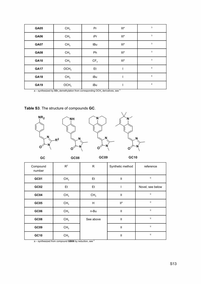
Table S3. The structure of compounds GC.

Compound number

R2 R Synthetic method reference

GC01 CH3 Et II 5

GC02 Et Et I Novel, see below

GC04 CH3 CH3 II 5

GC05 CH3 H IIa 5

GC06 CH3 n-Bu II 5

GC08 CH3 See above II 5

GC09 CH3 II 5

GC10 CH3 II 5

a – synthesized from compound GB08 by reduction, see 5

S13

(Z)-4-(4-(diethylamino)benzylidene)-2-ethyl-1-methyl-1H-imidazol-5(4H)-one (GC02).

4-(diethylamino)benzaldehyde 8.85 g (50 mmol), 2-propionamidoacetic acid 7.86 g (60 mmol) and sodium acetate 6.6 g (100 mmol) were dissolved in propionic anhydride (50 mL)/ The mixture was stirred at 110oC for 5 hours. The mixture was dissolved by EtOAc (400 mL), washed with water (2x150 mL) and brine (2x150 mL) and dried over Na2SO4. The solvent was evaporated and the product was purified by flash chromatography (Hexane- EtOAc 4:1). The residue was dissolved in ethanol (100 mL) and the methylamine solution (40% aq) was added. The mixture was stirred for 4 hours and the solvent was evaporated. The dimethylformamide (50 mL) and Cs2CO3 7.0 g (21 mmol) were added and the mixture was refluxed for 10 minutes. The solvent was evaporated and the mixture was dissolved by EtOAc (300 mL), washed with water (2x100 mL) and brine (2x100 mL) and dried over Na2SO4. The solvent was evaporated and the product was purified by column chromatography (CHCl3-EtOH 10:1).

Orange solid (5.99 g, 42%); mp = 141-144оС; 1H NMR (DMSO-d6) δ 8.07 (d, J=8.6 Hz, 2H), 6.85 (s, 1H), 6.72 (d, J=8.6 Hz, 2H), 3.42 (q, J=7.0 Hz, 4H), 3.07 (s, 3H), 2.65 (q, J=7.2 Hz, 2H), 1.26 (t, J=7.2 Hz, 3H), 1.12 (t, J=7.0 Hz, 6H); 13C NMR (DMSO-d6) δ 9.2 (CH3), 12.4 (CH3), 21.2 (CH2), 25.8 (CH2), 43.7 (CH3),111.0 (CH), 120.9, 126.5 (CH), 134.1 (CH), 134.2, 148.7, 163.4, 169.8; HRMS (ESI) m/z: 286.1921 found (calcd for C17H24N3O, [M+H]+ 286.1919).

Synthesis of the conformationally-locked compounds ABDI-BF2

ABDI-BF2 compounds were synthesized as reported previously 5 by the direct borylation of the corresponding imidazolones GC (Scheme S2). The synthetic procedures for all novel compounds are presented directly.

Scheme S2. General procedure of the borylation.

General method of ABDI-BF2 synthesis

Corresponding imidazol-5(4H)-one (GC) (10 mmol) was dissolved in dry CH2Cl2 (100 mL), molecular sieves 4Å (10 g) and 3Å (10 g) were added, followed by a solution of borone tribromide in CH2Cl2 (1М, 50 mL, 50.0 mmol) and the reaction mixture was refluxed for 2-8 hours in inert atmosphere. The mixture was cooled and filtered; molecular sieves were washed two times by ethanol (50 mL) and CH2Cl2 (300 mL). The solution was mixed with aqueous HF (20%, 10 mL) and stirred for 30 minutes. The mixture was dissolved by EtOAc (250 mL), washed with potassium carbonate solution (5%, 2x50mL), water (2x50 mL) and

S14

brine (2x50 mL) and dried over Na2SO4. The solvent was evaporated and the product was purified by column chromatography (CHCl3-EtOH).

Table S4. The structure of compounds ABDI-BF2.

Compound number R2 R reference

M739 CH3 Et 5

M774 Et Et Novel, see below

M766 CH3 CH3 5

M816 CH3 H 5

M1078 CH3 n-Bu 5

M1035 CH3 See above 5

M1169 CH3 5

M1167 CH3 5

(Z)-4-(4-(diethylamino)-2-(difluoroboryl)benzylidene)-2-ethyl-1-methyl-1H-imidazol-5(4H)-one (M774).

(Z)-4-(4-(diethylamino)benzylidene)-2-ethyl-1-methyl-1H-imidazol-5(4H)-one (GC02) 1.43 g (5.0 mmol) was dissolved in dry CH2Cl2 (50 mL), molecular sieves 4Å (4 g) and 3Å (4g) were added, followed by a solution of boron tribromide in CH2Cl2 (1М, 20 mL, 20.0 mmol) and the reaction mixture was refluxed for 6 hours in inert atmosphere. The mixture was cooled and filtered; molecular sieves were washed two times by ethanol (20 mL) and CH2Cl2 (100 mL). The solution was mixed with aqueous HF (20%, 5 mL) and stirred for 30 minutes. The mixture was dissolved by EtOAc (100 mL), washed with potassium carbonate solution (5%, 2x50mL), water (2x50 mL) and brine (2x50 mL) and dried over Na2SO4. The solvent was evaporated and the product was purified by column chromatography (CHCl3-EtOH 10:1).

Red solid (1.28 g, 77%); mp = 183-185оС; 1H NMR (DMSO-d6) δ 7.49 (s, 1H), 7.43 (d, J=8.8 Hz, 1H), 6.86 (d, J=2.2 Hz, 1H), 6.66 (dd, J1=8.8 Hz, J2=2.2 Hz, 1H), 3.47 (q, J=7.0

S15

Hz, 4H), 3.26 (s, 3H), 3.05 (q, J=7.7 Hz, 2H), 1.29 (t, J=7.7 Hz, 3H), 1.15 (t, J=7.0 Hz, 6H); 13C NMR (DMSO-d6) δ 10.6 (CH3), 12.5 (CH3), 19.4 (CH2), 26.2 (CH2), 43.9 (CH3), 110.6 (CH), 113.8 (CH), 121.1, 130.4 (CH), 134.7 (CH), 150.5, 162.3, 164.2; HRMS (ESI) m/z: 334.1884 found (calcd for C17H23BF2N3O, [M+H]+ 334.1902).

Molecular docking For preliminary molecular docking we followed previously published protocol6. Briefly, a library of lipocalin structures with two or one substitutions in amino acids facing potential binding site was generated with MODELLER software7 guided by published lipocalin structure (PDB ID: 1QWD). Files for the ligand (GFP chromophore) and receptor (lipocalin mutants) were prepared for docking in AutoDockTools8 version 1.5.6. Bounding box for docking was calculated in PyMol. Docking with rigid protein geometry was performed with AutoDock Vina9.

Molecular cloning The full copy of the crystallized fragment of the Blc protein10 was made in two stages. First, the shortened blc gene was amplified by nested polymerase chain reaction (PCR) from E. coli strain K12 Rosetta-gami 2(DE3)pLysS (external primer pair: Blc-F: 5’-ATGCCGTGTGGACGGGTATT-3’, Blc-R: 5’-CGCCGCCTGGCAGATTCTTA-3’; internal primer pair: Blc-Nhe-F: 5’-GTACGCTAGCAGCTCCACGCCGCCGCGTGGCGTGAC-3’, Blc-Hind-R: 5’-GTACAAGCTTCTAACTACCAGGCTGCTGTACCCAAATA-3’). The PCR fragment was cut with NheI/HindIII and ligated into NheI/HindIII-digested iRFP-pBAD vector instead of iRFP coding sequence. Then the missing linker sequence (Supplementary Figure 1a) between His-tag and the Blc protein fragment was added by self-assembling cloning 11 (Blc-link-F: 5’-AAGAAATCCAGCTCCACGCCGCCGC-3’, Blc-link-F-long: 5’-ACCAGCTTGTACAAGAAATCCAGCTCCACGCCGCCGC-3’, Blc-link-R: 5’-TGATTCGAGATGATGATGATGATGATGAGAACCC-3’, Blc-link-R-long: 5’-GTACAAGCTGGTTGATTCGAGATGATGATGATGATGATGAGAACCC-3’). Coding sequence of Blc-pBad was checked by sequencing and this vector was used for further work.

All 19 selected mutants differ from Blc in one or two amino acids. They were constructed either by one or by two rounds of self-assembling cloning11.

The H2B-TagBFP-Blc-mutant, actinin-Blc-mutant, and keratin-Blc-mutant plasmids for expression in mammalian cells were constructed by self-assembling cloning using Blc-mutant-pBAD and H2B-TagBFP (Evrogen), keratin-TagRFP (Evrogen) or actinin-TagRFP (Evrogen) vectors as a template.

The actinin-TagBFP-Blc-mutant and vimentin-TagBFP-Blc-mutant plasmids were made by standard digestion-ligation cloning approach. The TagBFP-Blc-mutant inserts were cut with AgeI/NotI from the H2B-TagBFP-Blc-mutant plasmids and ligated into AgeI/NotI-digested actinin-TagRFP (Evrogen) or vimentin-Citrine vector.

Protein expression and purification Blc and Blc-mutant proteins were expressed in XJb(DE3) Autolysis (Zymo Research) E. coli strain. One bacterial colony was inoculated into 200 ml of LB broth and grown overnight (~

S16

16 hours) at 37°C. Then 800 μl of 20% L-arabinose aqueous solution were added. After another 24 hours at 37°C cells were harvested and resuspended in 5 ml of PBS buffer (pH 7.4). Suspension was frozen at -70°C and thawed at 37°C three times. DNA was destroyed by short sonication, the lysate was centrifuged to obtain cell-free extract. The protein was purified using TALON metal affinity resin (Clontech). A fraction of beads with immobilized protein were aliquoted into a different tube while the rest was washed with PBS / 0.1M EDTA buffer (pH 7.4) to elute the protein into the solution. Finally, all purified samples were dialysed against PBS (pH 7.4).

Cell culture and transient transfection We have constructed a number of plasmids containing fusion proteins with selected Blc-mutants (H2B-TagBFP-blc16912, H2B-TagBFP-blc78776, keratin-blc16912, actinin-TagBFP-blc78776, actinin-blc16912, actinin-blc78776, vimentin-TagBFP-blc16912a, vimentin-TagBFP-blc16912, vimentin-TagBFP-blc78776) which were used for expression in human cell lines (HeLa Kyoto, NIH-3T3, and HEK293T) and subsequent confocal and wide-field fluorescence microscopy.

HeLa Kyoto, NIH-3T3 and HEK293T cells were grown in Dulbecco's modification of Eagle’s medium (DMEM) (PanEco) containing 50 U/ml penicillin and 50 µg/ml streptomycin (PanEco), 2 mM L-glutamine (PanEco) and 10% fetal bovine serum (HyClone, Thermo Scientific) at 37°C and 5% CO2. The day before transfection the cells were plated in 35mm Fluorodish cell culture dishes (WPI). For transient transfections the FuGENE 6 transfection reagent (Roche) was used according to protocol. Cells were imaged 24 - 48 hours after transfection. Before imaging the cells were washed two times with Versene solution (PanEco) and imaged in Hank’s balanced salt solution (PanEco) or minimum essential medium Eagle (MEM) (Sigma), both supplemented with 20 mM HEPES (PanEco).

Fluorescence microscopy Primary protein-fluorophore interaction screening was performed with TALON beads. Dialysed Blc-mutant protein containing beads (or free TALON beads as a control) were placed in wells of a 96-well plate with 100 μl of PBS buffer. Then the solutions of fluorophores were added to obtain 10 μM concentration. After 10-min incubation at RT the beads were imaged by using BZ-9000 fluorescence microscope (Keyence) with a 2x objective, OP-79301 SB GFP-BP and OP-79302 SB TexasRed filters, and equal exposure time.

Widefield fluorescence microscopy was performed with tthe BZ-9000 fluorescence microscope (Keyence) with a 40x objective (filter sets OP-79301 SB GFP-BP and OP-79302 SB TexasRed). Confocal imaging presented in the Manuscript (Figure 1) as well as the bleaching experiments (Figure 2b) was performed using an inverted Leica confocal microscope DMIRE2 TCS SP2 (Leica, Wetzlar, Germany) equipped with HCX PL APO lbd.BL 63.0x1.40 OIL objective, excitation by 488 nm laser line (100 µW) , detection at 500-530 nm (DiB1, DiB2), or by 543 laser line (20 µW), detection at 550-600 nm (DiB3).

Single-molecule localization super-resolution imaging of living cells was carried out on a Nikon Eclipse Ti N-STORM microscope (Nikon, Japan) controlled by NIS-Elements

S17

Software and/or the Micro-Manager software12. The excitation light from 488 nm (4.5 W/cm2) or 561 nm (120 W/cm2) laser lines was focused on the sample with a 100X oil-immersion objective (Apo TIRF/1.49, Nikon) and PFS (perfect focus system). Optical path included C-NSTORM QUAD filter cube (Nikon) and a 1.5x magnifier lens. The images (a pixel size of 107 nm) were captured with the EM-CCD camera (iXon3 DU-897, Andor, UK) at 10 MHz readout rate, 14-bit, with an EM gain and a pre-amplifier gain set to 200 and 5.1 (12.15 electrons per A/D count) respectively, with an exposure time of 16-50 ms. The TIRF illuminator mirror was adjusted to allow for total internal reflection (objective-based TIRF). A typical series of 5000 frames was taken using ND Acquisition mode. The running median filtering was applied to the time series prior to localization step13. Sparse images of individual fluorophores were fitted with the ThunderStorm2 plugin for FIJI14. Localization uncertainties reported here are calculated by ThunderStorm2 following EM-CCD optimized formula1.

Single-molecule localization with high-power illumination was carried out on Leica SR GSDIM system, equipped with the EM-CCD camera (Andor iXon 3 897), SuMo stabilized stage, HCX PL APO 100x/1.47 OIL objective with additional 1.6x magnification (96 nm effective pixel size). The sample was illuminated with 488 laser line operating in “epi” mode (straight out of the objective”) at the power density of 5 kW/cm2. The camera exposure time was set to 10 ms. Camera settings: 10 MHz readout rate, 14-bit, pre-amplifier gain 5 (12.15 electrons per A/D count), EM gain 296.

STED microscopy was performed on Leica TCS SP8 STED 3X in a Gated-STED mode with Hybrid detectors and HC PL APO CS2 93x/1.30 glycerine-immersion objective. The 514 nm line of the tunable White Light Laser was used for fluorophore excitation at 40% output power. Fluorescence depletion by stimulated emission was achieved with the 40% output power of 1.44W 592 nm continuous-wave laser.

Cell perfusion experiments (Figure 2a) were performed on the Leica AF6000B imaging system equipped with ZYLA-5.5-CL10 camera (Andor, UK), controlled by the Micro-Manager software12. The HBSS solution or HBSS with the M739 (0.5 µM) were pumped into the imaging chamber of the µ-Slide VI 0.4 (IBIDI, Germany) with the Milliliter Syringe Pump Module (Harvard Apparatus, USA) controlled via serial port. The excess of the fluid was removed by the peristaltic pump.

Chromophore titration To investigate the binding of fluorophores to Blc-mutant proteins, fluorescence titration was performed. The data were obtained using newly purificated and dialysed protein, and newly diluted fluorophore solutions.

Samples of dry fluorophore were diluted in DMSO. These solutions were used for subsequent preparation of the 1000X stock solutions in 96% EtOH. The concentration of the fluorophores in the stock solutions was measured using Cary 100 UV/VIS spectrophotometer, and the 100X working solutions in PBS buffer were made before each titration. The concentration of the proteins was evaluated using sample absorption at 280 nm and extinction coefficients computed by ProtParam tool (http://web.expasy.org/protparam/). To reduce dilution-induced artifacts during titration, series of diluted protein solutions were also prepared.

The fluorophore solution (10 μl) and required amount of protein solution and PBS up

S18

to 1 ml were added into cuvette, gently stirred and immediately measured using Varian Cary Eclipse fluorescence spectrophotometer. For each fluorophore-protein pair points with at least two different fluorophore and fifteen protein concentrations were measured.

Analysis of fluorescence titration data The fluorescence titration data were fitted to the 1:1 binding model. Supposing Blc-mutant proteins as monomers with single binding site for fluorophore, the binding of fluorophore to Blc-mutant protein can be described as P + F ⇌ PF, where P is free protein, F is free fluorophore, and PF is protein-fluorophore complex. Then the dissociation constant (Kd) equation is:

, Kd = [PF ]eq[P ] [F ]eq eq

where [P]eq is free protein, [F]eq is free fluorophore, and [PF]eq is protein-fluorophore concentrations at equilibrium.

As we knew only initial concentration of the protein and the fluorophore, and had not any tool for the free protein and the free fluorophore concentration at equilibrium measurement, the Kd equation was rewritten using mass balance equations:

[P]init = [P]eq + [PF]eq

[F]init = [F]eq + [PF]eq

where [P]init and [F]init are initial concentration of the protein and the fluorophore, respectively: [P]eq = [P]init - [PF]eq [F]eq = [F]init - [PF]eq

Kd = [PF ]eq([P ] − [PF ] )([F ] − [PF ] )init eq init eq

= [P ] [PF ] )([F ] [PF ] )( init − eq init − eq [PF ]Kd eq P ] [F ] [PF ] [F ] [P ] [PF ] PF ] [PF ] 0 [ init init − eq init − init eq + [ 2

eq − Kd eq = [PF ] [PF ] ([F ] [P ] ) P ] [F ] 0 2

eq − eq init + init + Kd + [ init init = The protein-fluorophore complex ([PF]eq) concentration can be expressed as:

(1)PF ] [ eq = 2([F ] + [P ] +K ) − init init d √([F ] + [P ] +K ) − 4[P ] [F ]init init d

2init init

Thus the fluorescence emission intensity (F) of the protein-fluorophore solution can be expressed as:

(2) PF ] [F ] [PF ] ) F = [ eq * Φ[PF ] + ( init − eq * Φ[F ] where Φ[PF] and Φ[F] are the relative fluorescence quantum yields of the protein-fluorophore complex and the pure fluorophore, respectively.

Therefore to determine apparent Kd, the experimentally obtained data were fitted to equation 2 by leastsq method from Scipy optimize package.

Quantum yield measurement Quantum yield of the protein-fluorophore complexes was determined by direct comparison with purified EGFP protein (quantum yield 0.6).

S19

Supplementary references 1 T. Quan, S. Zeng and Z.-L. Huang, J. Biomed. Opt., 2010, 15, 066005. 2 M. Ovesný, P. Křížek, J. Borkovec, Z. Svindrych and G. M. Hagen, Bioinformatics, 2014,

30, 2389–2390. 3 M. S. Baranov, K. M. Solntsev, K. A. Lukyanov and I. V. Yampolsky, Chem. Commun. ,

2013, 49, 5778–5780. 4 M. S. Baranov, I. T. Fedyakina, M. Y. Shchelkanov and I. V. Yampolsky, Tetrahedron,

2014, 70, 3714–3719. 5 M. S. Baranov, K. M. Solntsev, N. S. Baleeva, A. S. Mishin, S. A. Lukyanov, K. A.

Lukyanov and I. V. Yampolsky, Chem. Eur. J., 2014, 20, 13234–13241. 6 N. V. Povarova, N. G. Bozhanova, K. S. Sarkisyan, R. Gritcenko, M. S. Baranov, I. V.

Yampolsky, K. A. Lukyanov and A. S. Mishin, J. Mater. Chem., 2016, 4, 3036–3040. 7 B. Webb and A. Sali, in Current Protocols in Bioinformatics, John Wiley & Sons, Inc.,

2002. 8 G. M. Morris, R. Huey, W. Lindstrom, M. F. Sanner, R. K. Belew, D. S. Goodsell and A.

J. Olson, J. Comput. Chem., 2009, 30, 2785–2791. 9 O. Trott and A. J. Olson, J. Comput. Chem., 2010, 31, 455–461. 10 V. Campanacci, D. Nurizzo, S. Spinelli, C. Valencia, M. Tegoni and C. Cambillau, FEBS

Lett., 2004, 562, 183–188. 11 A. Matsumoto and T. Q. Itoh, Biotechniques, 2011, 51, 55–56. 12 A. D. Edelstein, M. A. Tsuchida, N. Amodaj, H. Pinkard, R. D. Vale and N. Stuurman, J

Biol Methods, , DOI:10.14440/jbm.2014.36. 13 E. Hoogendoorn, K. C. Crosby, D. Leyton-Puig, R. M. P. Breedijk, K. Jalink, T. W. J.

Gadella and M. Postma, Sci. Rep., 2014, 4, 3854. 14 J. Schindelin, I. Arganda-Carreras, E. Frise, V. Kaynig, M. Longair, T. Pietzsch, S.

Preibisch, C. Rueden, S. Saalfeld, B. Schmid, J.-Y. Tinevez, D. J. White, V. Hartenstein, K. Eliceiri, P. Tomancak and A. Cardona, Nat. Methods, 2012, 9, 676–682.

S20