Supplementary Information for“Reducing Cascading Failure Risk by IncreasingInfrastructure Network Interdependence”Mert Korkali, Jason G. Veneman, Brian F. Tivnan, James P. Bagrow, and Paul D.H. Hines

Supplementary NoteDC power-flow modelIn this paper, we made use of the “DC power flow” linearization of the full nonlinear power flow equations in our modelof cascading failures. Here, we briefly describe the derivation of this common, although imperfect, simplification. For amore detailed discussion of the DC power-flow equations and their limitations, see refs S1, S2.

Consider a node (“bus” in power systems terminology) k that is connected to node m via a transmission line, whichhas series resistance rkm and reactance xkm = ωlkm, where ω is the frequency of the sinusoidal current and lkm is theseries inductance of the line. r and x can be combined to form a complex impedance zkm = rkm + jxkm, in which (byelectrical engineering notational tradition) j =

√−1. The inverse of this impedance is known as an “admittance,”

and is defined as follows: 1/zkm = ykm = gkm + jbkm, where g and b are known, respectively, as the conductance andsusceptance of the line. The sinusoidal voltages at nodes k and m will each have an amplitude (V ) and a phase shift (θ ,relative to some reference), and can thus be represented with complex numbers Vk =Vke jθk and Vm =Vme jθm . Note thatvoltages Vk, and consequently all other units, are normalized to dimensionless units, using the ‘per-unit’ system, suchthat 1.0 indicates a nominal value. With these definitions, we can define the complex current I and power Sflowing outfrom k to m as:

Ikm = ykm(Vk−Vm) (S1)

Skm = VkI∗km = Vk(V ∗k −V ∗m)y∗km (S2)

where x∗ indicates the complex conjugate of x. With some manipulation of equations (S1) and (S2), we can find theactive (P) and reactive (Q) power flowing from k to m as follows:

Pkm =V 2k gkm−VkVm(gkm cosθkm +bkm sinθkm) (S3)

Qkm =−V 2k bkm−VkVm(gkm sinθkm−bkm cosθkm) (S4)

where θkm = θk−θm is the phase angle difference between k and m. If we assume that the voltage amplitudes Vk and Vmare at their nominal levels, that we have normalized ykm such that this nominal level is 1.0 (common practice), and thatthe resistance rkm is small (nearly zero) relative to the reactance xkm (a reasonable assumption for bulk power systems),then gkm ∼= 0, and Pkm becomes:

Pkm ∼=−bkm sinθkm =1

xkmsinθkm (S5)

If we assume that θkm is small, then sinθkm ∼= θkm and we get:

Pkm ∼=1

xkmθkm (S6)

If we furthermore assume that Qkm = 0 (not a particularly good assumption), then the current magnitude and the powerare equal, |Ikm|=Pkm, and we can use equation (S6) to roughly simulate power flows in a power system.

In order to solve for the flows Pkm in simulation, we put equation (S6) into matrix form as follows. Let A denotethe line-to-node incidence matrix with 1 and −1 in each row indicating the endpoints of each line, θ be the vectorof voltage phase angles, X be a diagonal matrix of line reactances, and Pflow be a vector of active power flows along

1

transmission lines. Then, we can solve for the vector of power flows Pflow given that we know the vector of voltagephase angles θ as shown in the following:

A>θ = XPflow (S7)

Pflow =[X−1A>

]θ (S8)

In order to solve for θ , we use information about the sources (generators) and sinks (loads) to build a vector of netinjected powers (generation minus load), P. Given P, we can solve the following to find θ :

P= APflow =[AX−1A>

]θ = Bθ (S9)

The matrix B is known as the bus susceptance matrix, and has the properties of a weighted graph Laplacian matrixdescribing the network of transmission lines, where the link weights are the susceptances bkm = 1/xkm.

Comparing PN/2 to P∞

In this paper, we measured the impact of disturbances of various sizes, f , on the probability of at least half of thenetwork remaining within the “giant component” (GC) after the resulting cascade had subsided: PN/2; or the probabilityof half of the load still being served after the cascade completed: PD/2. An alternative way to measure the impact ofthe disturbances is to measure the average cascade size (sometimes known as the yield), rather than the probability ofa cascade in a given size range. Indeed, after random removal of f N nodes from the network, N0 = (1− f )N nodesremain in the GC, and the cascade of failures results in gradual fragmentation of the network, leading to a reduction inthe number of nodes in the GC until a post-cascade steady state is reached. At this point, we calculated the ratio of thenumber of nodes remaining within the end-state GC, N∞, to the size of the network after the initial removal of nodes,N0, and measured the average cascade size, 〈N∞/N0〉, across a set of samples. This measure would be more analogousto the P∞-metric that is commonly used in the literature on phase transitions in percolation systems. We chose not to useP∞ as our primary measure of network robustness since the modeling assumptions described in the above discussion of“DC power flow” become particularly inaccurate for very large cascades. Essentially, P∞ would, in many cases, averageover small numbers that were not particularly accurate.

However, the results that one obtains by measuring the average cascade impact do not lead one to substantiallydifferent conclusions than those reported in the paper (aside from the fact that the transitions are much more gradual).

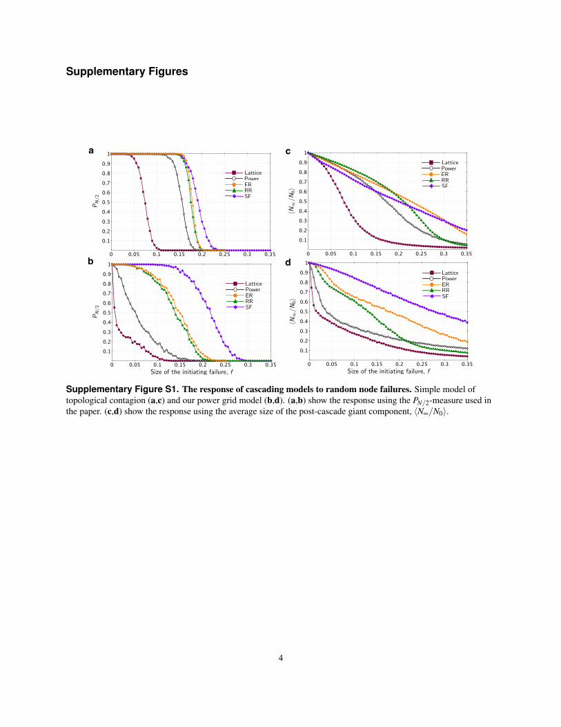
Supplementary Figure S1 compares the response of various networks to random failures using the P∞- and PN/2-measures for the topological contagion and power grid models. For the power grid model, the relative robustness ofthe five network structures is unchanged. The lattice is the most vulnerable and the scale-free network is the mostrobust. In the topological model, the P∞-measure indicates that the power grid, random graph, random regular, andscale-free networks have similar levels of robustness, for f < 0.15. The lattice remains to be the most vulnerable of thefive network structures.

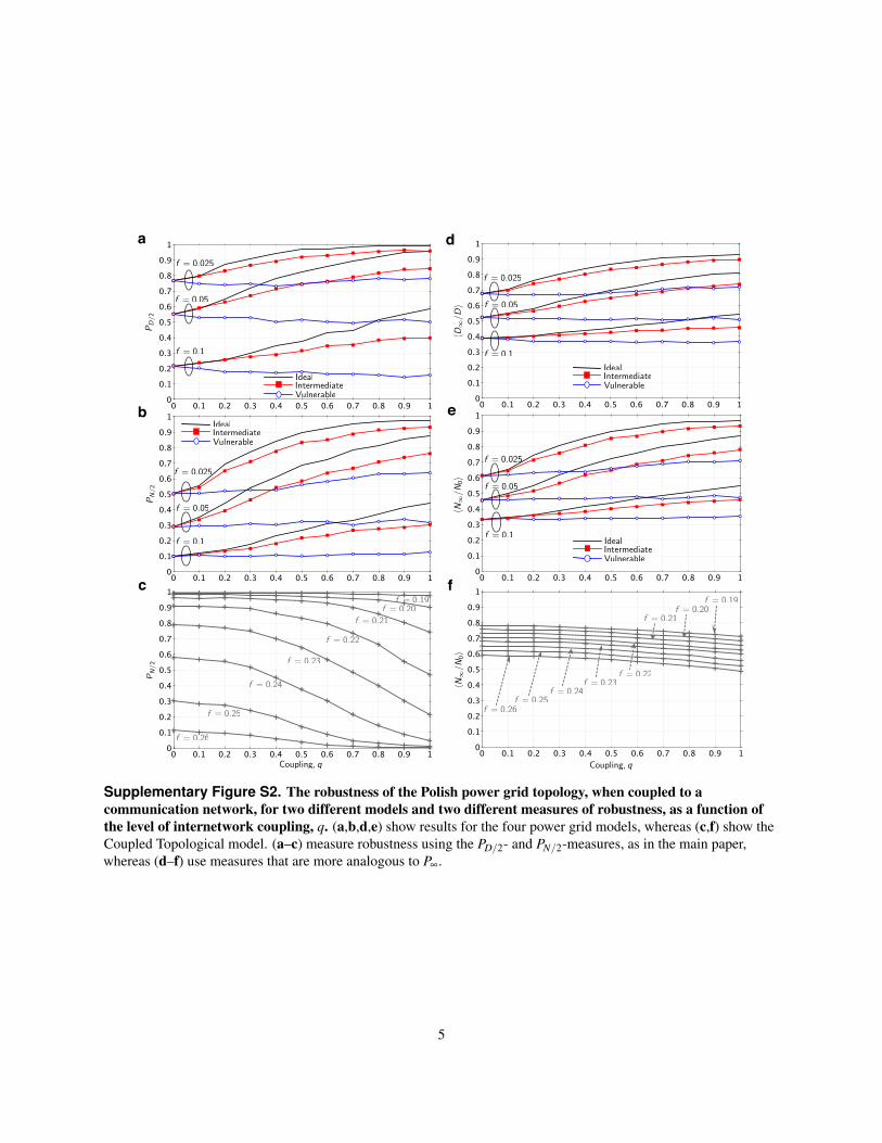
Supplementary Figure S2 compares the response of various coupled models to random failures with different levelsof coupling between the power and communications network. In this case, we compare the original metrics used inthe paper (i.e., PN/2 and PD/2) to P∞. Our analogous measure of robustness for the three smart grid models is 〈D∞/D〉:the average ratio of the amount of demand (load) served at the end of the cascade to the original load, which amountsto 24.5725 GW. The results for the three different smart grid models are not substantially changed. We still see thatincreased coupling increases robustness in both the Ideal and the Intermediate Smart Grid models, whereas coupling isdetrimental (though only slightly) in the Vulnerable Smart Grid model. For the Coupled Topological model, coupling isdetrimental to robustness; indeed, by measuring the results using both P∞ and PN/2, the decrease in performance with qis monotonic.

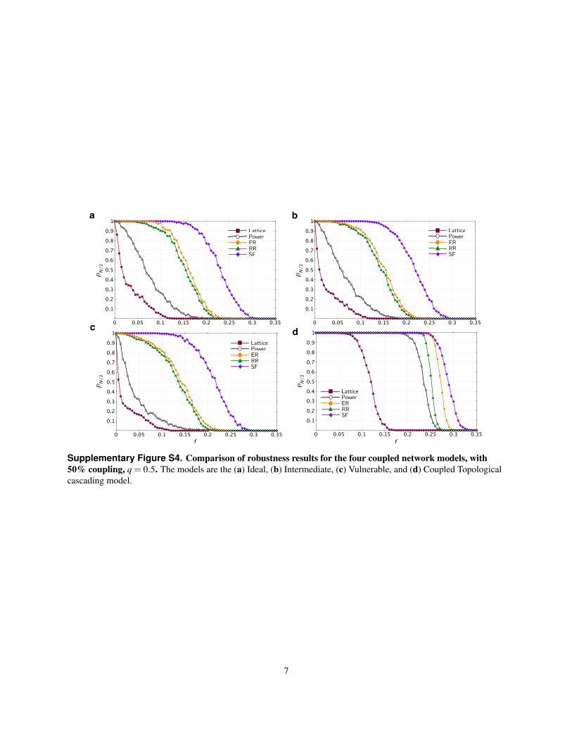
50% coupling resultsTo better understand the impact of the level of coupling, we recomputed the results shown in Supplementary Fig. S4using 50% coupling, i.e., q = 0.5.

2

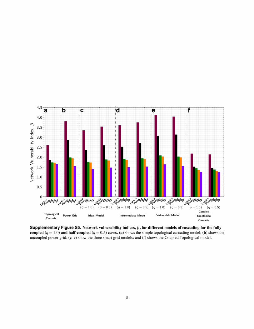
Network vulnerability indicesOne way to compare the various topological configurations and models described in this paper is to convert the sigmoidalresults shown in Supplementary Figs S3 and S4 into a single metric of robustness (or conversely, vulnerability). Toquantify the effects of topology, physics, and coupling among different synthetic networks, we define the networkvulnerability index (β ) as follows:

β =− log∫ 1

0PGC( f ) d f (S10)

≈− log{

12L

L−1

∑`=1

PGC( f`)+PGC( f`+1)

}(S11)

where f is the initiating failure size; L is the total number of f values simulated; and PGC = PN/2 is the probability ofobserving a GC whose size is more than half the number of grid nodes. The β -values corresponding to five networkstructures and six models of cascading studied in this paper are aggregately displayed in a bar chart in SupplementaryFig. S5.

Sensitivity analysis on λ

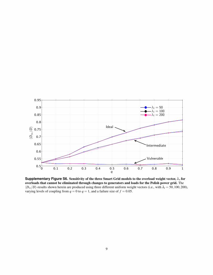
Sensitivity of the three smart grid models with respect to the weight vector λ using various levels of coupling rangingfrom q = 0 to q = 1 is displayed in Supplementary Fig. S6. This analysis is carried out using our load-based P∞-measure,in which the ratios of the amount of post-cascade power, D∞, to the precascade load amount, D, are averaged across thesame 1,000 initial outage sets of failure size f = 0.05, as in other cases. It is clearly seen that the choice of the weightvector, λ , of unavoidable overloads has only negligible impact on the values of the chosen robustness metric, 〈D∞/D〉.

Supplementary ReferencesS1. Stott, B., Jardim, J. & Alsac, O. DC power flow revisited. IEEE Trans. Power Syst. 24, 1290–1300 (2009).

S2. Gómez-Expósito, A., Conejo, A. J. & Cañizares, C. (eds.) Electric Energy Systems: Analysis and Operation (CRCPress, Baco Raton, FL, 2009).

3

Supplementary Figures

0.350 0.05 0.1 0.15 0.2 0.25 0.3

1

0.10.20.30.40.50.60.70.80.9

1

0.10.20.30.40.50.60.70.80.9

0.350 0.05 0.1 0.15 0.2 0.25 0.3

hN1

/N0i

hN1

/N0i

Size of the initiating failure, f

c

d

ERPower

SF

Lattice

RR

ERPower

SF

Lattice

RR

0.350 0.05 0.1 0.15 0.2 0.25 0.3

1

0.10.20.30.40.50.60.70.80.9

0.350 0.05 0.1 0.15 0.2 0.25 0.3

1

0.10.20.30.40.50.60.70.80.9

PN

/2

PN

/2

Size of the initiating failure, f

a

b

ERPower

SF

Lattice

RR

ERPower

SF

Lattice

RR

Supplementary Figure S1. The response of cascading models to random node failures. Simple model oftopological contagion (a,c) and our power grid model (b,d). (a,b) show the response using the PN/2-measure used inthe paper. (c,d) show the response using the average size of the post-cascade giant component, 〈N∞/N0〉.

4

10 0.1 0.2 0.3 0.4 0.5 0.6 0.7 0.8 0.9

1

00.10.20.30.40.50.60.70.80.9

1

00.10.20.30.40.50.60.70.80.9

0 0.90.50.1 0.6 10.2 0.70.3 0.80.4

1

00.10.20.30.40.50.60.70.80.9

0 0.90.50.1 0.6 10.2 0.70.3 0.80.4

1

00.10.20.30.40.50.60.70.80.9

0 0.90.50.1 0.6 10.2 0.70.3 0.80.4

1

00.10.20.30.40.50.60.70.80.9

0 0.90.50.1 0.6 10.2 0.70.3 0.80.4

10 0.1 0.2 0.3 0.4 0.5 0.6 0.7 0.8 0.9

1

00.10.20.30.40.50.60.70.80.9

PD

/2

Coupling, q

PN

/2

a

c

f = 0.24

f = 0.23

f = 0.22

f = 0.20

f = 0.25

f = 0.26

f = 0.21

f = 0.19

f = 0.05

IntermediateIdeal

Vulnerable

f = 0.05

PN

/2

IntermediateIdeal

Vulnerable

b

Coupling, q

hN1

/N0i

f

f = 0.24f = 0.23

f = 0.22

f = 0.20

f = 0.25f = 0.26

f = 0.21

f = 0.19

IntermediateIdeal

Vulnerable

f = 0.05

hN1

/N0i

hD1

/Di

d

f = 0.05

IntermediateIdeal

Vulnerable

e

f = 0.025

f = 0.1

f = 0.025

f = 0.1

f = 0.025

f = 0.1

f = 0.025

f = 0.1

Supplementary Figure S2. The robustness of the Polish power grid topology, when coupled to acommunication network, for two different models and two different measures of robustness, as a function ofthe level of internetwork coupling, q. (a,b,d,e) show results for the four power grid models, whereas (c,f) show theCoupled Topological model. (a–c) measure robustness using the PD/2- and PN/2-measures, as in the main paper,whereas (d–f) use measures that are more analogous to P∞.

5

0.350 0.05 0.1 0.15 0.2 0.25 0.3

1

0.10.20.30.40.50.60.70.80.9

0.350 0.05 0.1 0.15 0.2 0.25 0.3

1

0.10.20.30.40.50.60.70.80.9

0.350 0.05 0.1 0.15 0.2 0.25 0.3

1

0.10.20.30.40.50.60.70.80.9

0.350 0.05 0.1 0.15 0.2 0.25 0.3

1

0.10.20.30.40.50.60.70.80.9

0.350 0.05 0.1 0.15 0.2 0.25 0.3

1

0.10.20.30.40.50.60.70.80.9

0.350 0.05 0.1 0.15 0.2 0.25 0.3

1

0.10.20.30.40.50.60.70.80.9

f f

a b

c d

e f

ERPower

SF

Lattice

RRERPower

SF

Lattice

RR

ERPower

SF

Lattice

RRERPower

SF

Lattice

RR

ERPower

SF

Lattice

RR

ERPower

SF

Lattice

RR

PN

/2

PN

/2

PN

/2

PN

/2

PN

/2

PN

/2

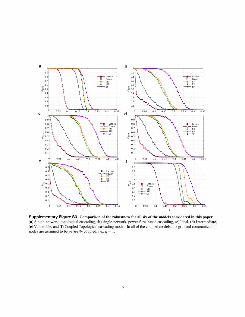
Supplementary Figure S3. Comparison of the robustness for all six of the models considered in this paper.(a) Single-network, topological cascading, (b) single-network, power-flow-based cascading, (c) Ideal, (d) Intermediate,(e) Vulnerable, and (f) Coupled Topological cascading model. In all of the coupled models, the grid and communicationnodes are assumed to be perfectly coupled, i.e., q = 1.

6

0.350 0.05 0.1 0.15 0.2 0.25 0.3

1

0.10.20.30.40.50.60.70.80.9

0.350 0.05 0.1 0.15 0.2 0.25 0.3

1

0.10.20.30.40.50.60.70.80.9

0.350 0.05 0.1 0.15 0.2 0.25 0.3

1

0.10.20.30.40.50.60.70.80.9

0.350 0.05 0.1 0.15 0.2 0.25 0.3

1

0.10.20.30.40.50.60.70.80.9

f f

a b

c d

ERPower

SF

Lattice

RRERPower

SF

Lattice

RR

ERPower

SF

Lattice

RR

ERPower

SF

Lattice

RR

PN

/2

PN

/2

PN

/2

PN

/2

Supplementary Figure S4. Comparison of robustness results for the four coupled network models, with50% coupling, q = 0.5. The models are the (a) Ideal, (b) Intermediate, (c) Vulnerable, and (d) Coupled Topologicalcascading model.

7

4.5

0

1.0

2.0

3.0

4.0

0.5

1.5

2.5

3.5

Lattice

Powe

rSFER

Net

wor

kVuln

erab

ility

Index

,�

RR

Lattice

Powe

rSFERRR

Lattice

Powe

rSFERRR

Lattice

Powe

rSFERRR

Lattice

Powe

rSFERRR

Lattice

Powe

rSFERRR

Topological

Cascade

Coupled

Power GridTopological

Cascade

a b c d e f

Lattice

Powe

rSFERRR

Lattice

Powe

rSFERRR

Lattice

Powe

rSFERRR

Lattice

Powe

rSFERRR

(q = 1.0) (q = 0.5) (q = 1.0) (q = 0.5) (q = 1.0) (q = 0.5) (q = 1.0) (q = 0.5)

Ideal Model Intermediate Model Vulnerable Model

Supplementary Figure S5. Network vulnerability indices, β , for different models of cascading for the fullycoupled (q = 1.0) and half-coupled (q = 0.5) cases. (a) shows the simple topological cascading model; (b) shows theuncoupled power grid; (c–e) show the three smart grid models; and (f) shows the Coupled Topological model.

8

10 0.1 0.2 0.3 0.4 0.5 0.6 0.7 0.8 0.9

0.95

0.5

0.55

0.6

0.65

0.7

0.75

0.8

0.85

0.9

q

�i = 100�i = 50

�i = 200

Ideal

Intermediate

Vulnerable

hD1

/Di

Supplementary Figure S6. Sensitivity of the three Smart Grid models to the overload weight vector, λ , foroverloads that cannot be eliminated through changes to generators and loads for the Polish power grid. The〈D∞/D〉-results shown herein are produced using three different uniform weight vectors (i.e., with λi = 50,100,200),varying levels of coupling from q = 0 to q = 1, and a failure size of f = 0.05.

9