Supplemental Appendix 1 - inferring SNVs from … · Supplemental Appendix 1 - inferring SNVs from aligned reads using a Bayesian mixture model Sohrab P. Shah, Ryan D. Morin and Samuel

SUPPLEMENTARY INFORMATION

1www.nature.com/nature

doi: 10.1038/nature08489

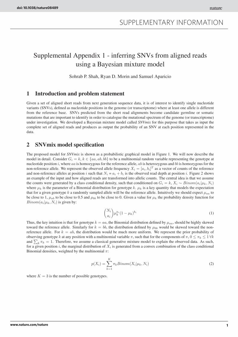
Supplemental Appendix 1 - inferring SNVs from aligned readsusing a Bayesian mixture model

Sohrab P. Shah, Ryan D. Morin and Samuel Aparicio

1 Introduction and problem statementGiven a set of aligned short reads from next generation sequence data, it is of interest to identify single nucleotidevariants (SNVs), defined as nucleotide positions in the genome (or transcriptome) where at least one allele is differentfrom the reference base. SNVs predicted from the short read alignments become candidate germline or somaticmutations that are important to identify in order to catalogue the mutational spectrum of the genome (or transcriptome)under investigation. We developed a Bayesian mixture model called SNVmix for this purpose that takes as input thecomplete set of aligned reads and produces as output the probability of an SNV at each position represented in thedata.

2 SNVmix model specificationThe proposed model for SNVmix is shown as a probabilistic graphical model in Figure 1. We will now describe themodel in detail. Consider Gi = k, k ∈ {aa, ab, bb} to be a multinomial random variable representing the genotype atnucleotide position i, where aa is homozygous for the reference allele, ab is heterozygous and bb is homozygous for thenon-reference allele. We represent the observed allele frequency Xi = [ai, bi]T as a vector of counts of the referenceand non-reference alleles at position i such that Ni = ai + bi is the observed read depth at position i. Figure 2 showsan example of the input and how aligned reads are transformed into allelic counts. The central idea is that we assumethe counts were generated by a class conditional density, such that conditioned on Gi = k, Xi ∼ Binom(ai|µk, Ni)where µk is the parameter of a Binomial distribution for genotype k. µk is a key quantity that models the expectationthat for a given genotype k a randomly sampled allele will be the reference allele. Intuitively we should expect µaa tobe close to 1, µab to be close to 0.5 and µbb to be close to 0. Given a value for µk the probability density function forBinom(ai|µk, Ni) is given by:

Ni

ai

µai

k (1− µk)bi (1)

Thus, the key intuition is that for genotype k = aa, the Binomial distribution defined by µaa, should be highly skewedtoward the reference allele. Similarly for k = bb, the distribution defined by µbb would be skewed toward the non-reference allele. For k = ab, the distribution would be much more uniform. We represent the prior probability ofobserving genotype k at any position with a multinomial variable π, such that for the components of π, 0 ≤ πk ≤ 1 ∀kand

k πk = 1. Therefore, we assume a classical generative mixture model to explain the observed data. As such,

for a given position i, the marginal distribution of Xi is generated from a convex combination of the class conditionalBinomial densities, weighted by the multinomial π:

p(Xi) =K

k=1

πkBinom(Xi|µk, Ni) (2)

where K = 3 is the number of possible genotypes.

1


doi: 10.1038/nature08489 SUPPLEMENTARY INFORMATION

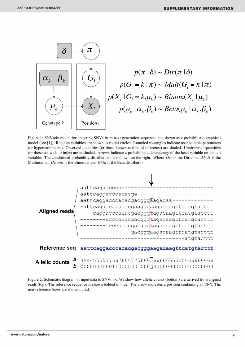
Figure 1: SNVmix model for detecting SNVs from next generation sequence data shown as a probabilistic graphicalmodel (see [1]). Random variables are shown as round circles. Rounded rectangles indicate user settable parameters(or hyperparameters). Observed quantities (or those known at time of inference) are shaded. Unobserved quantities(or those we wish to infer) are unshaded. Arrows indicate a probabilistic dependency of the head variable on the tailvariable. The conditional probability distributions are shown on the right. Where Dir is the Dirichlet, Mult is theMultinomial, Binom is the Binomial and Beta is the Beta distribution.

Figure 2: Schematic diagram of input data to SNVmix. We show how allelic counts (bottom) are derived from alignedreads (top). The reference sequence is shown bolded in blue. The arrow indicates a position containing an SNV. Thenon-reference bases are shown in red.

2


SUPPLEMENTARY INFORMATIONdoi: 10.1038/nature08489

Therefore the complete data log-likelihood is given by:

log p(X1:T |µ1:K , π) =Ti=1

logKk=1

πkBinom(Xi|µk, Ni) (3)

where T is the number of observed positions in the input.The parameters θ = (π, µ1:K) are fit to data using maximum a posteriori (MAP) expectation maximization (EM).

If the true genotype is known, θ can be learned in a supervised setting using the true genotypes as training data. Ourgoal is to infer the genotype state given the model parameters and the data. We can make use of Bayes rule and expressγi(k) = p(Gi = k|X1:N , π, µk) as the marginal probability of the genotype for position i given all the data and themodel parameters:

γi(k) =πkBinom(Xi|µk, Ni)Kj=1 πjBinom(Xi|µj , Ni)

(4)

3 Prior distributionsWe assume that π is distributed according to a Dirichlet distribution parameterized by δ, the so-called pseudocounts.We set delta to be skewed towards πaa under the assumption that most positions will be homozygous for the referenceallele. µk is conjugately distributed according to a Beta distribution: µk ∼ Beta(µk|αk, βk). We set αaa=1000,βaa=1; αab = 500, βab = 500 and αbb = 1,βbb = 1000 assuming that the µaa should be near close to 1, µab shouldbe close to 0.5 and µbb should be close to 0.

4 Model fitting and parameter estimationWe fit the model using the expectation maximization (EM) algorithm. In order to begin EM the model parametersmust be initialised. We initialise µk by taking the mean of 1000 random samples from the Binomial parameterized byµ̂k = αk

αk+βk. π(k) is initialised to δ(k)

Nδwhere Nδ =

k δ(k).

The EM algorithm iterates between the E-step where we assign the genotypes using Equation 4 and the M-stepwhere we re-estimate the model parameters. At each iteration we evaluate Equation 3 and the algorithm terminateswhen this quantity no longer increases.

The M-step equations are standard conjugate updating equations:

πnew(k) =T

i=1 I(Gi = k) + δ(k)j

Ti=1 I(Gi = j) + δ(j)

(5)

where I(Gi = k) is an indicator function to signal that Gi is assigned to state k as position i, and:

µnewk =T

i=1 aI(Gi=k)i + αkT

i=1 NI(Gi=k)i + αk + βk − 2

(6)

5 Evaluation of modelWe evaluated the performance of SNVmix by running it to convergence using 15000 coding positions determinedby using data from an orthogonal assay, namely genotype calls from an Affymetrix SNP 6.0 genotyping array. Welimited the positions by only considering coding positions where the CRLMM algorithm [2] predicted genotype with> 0.99 confidence. We therefore defined any position that was predicted to be heterozygous or homozygous for thenon-reference allele to be a true positive (TP) and any position predicted to be homozygous for the reference allele atrue negative (TN). We then computed p(SNVi) = γi(ab) + γi(bb) representing the posterior marginal probability ofan SNV at position i as predicted by the model. This allowed us to compute standard receiver operator characteristic(ROC) curves in order to quantitatively assess performance. We fit the model separately for WTSS-PE and WGSS-PE

3



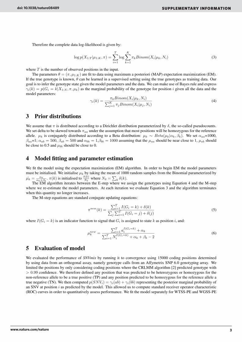
WGSS-PE AUC = 0.985 WTSS-PE AUC = 0.976

Figure 3: ROC curves of SNVMix predictions compared against high confidence genotype calls from an AffymetrixSNP 6.0 array. The WGSS-PE (left) and WTSS-PE (right) indicate the algorithm is highly concordant with theorthogonally derived results from the SNP chip.

using the set of positions described above and computed p(SNV1:T ) for each set of data. The resulting ROC curvesare shown in Figure 3 and demonstrate the algorithm is highly concordant with the high-confidence genotype callsfrom the SNP chip for both WGSS-PE (left) and WTSS-PE (right).

6 Computation of SNVs and selection criteria for validationUsing the converged parameter estimates from the model fits (described above) we evaluated Equation 4 for all the datafor WTSS-PE, WGSS-PE and WGSS-PRI. We chose to call an SNV as such by determining threshold probability t atthe 0.01 false positive rate. This was t = 0.53 for WTSS-PE and t = 0.77 for WGSS-PE. We applied these thresholdsso that locations where P (SNVi) > t were ’called’ SNVs. We then filtered out any SNVs that were present indbSNP v129, Jim Watson, Craig Venter, the Yoruban male and data from the 1000 genomes project as described inthe Supplemental Methods. The remaining SNVs were categorized according whether or not they induced a non-synonymous change. All non-synonymous changes were selected for validation by PCR amplicon sequencing.

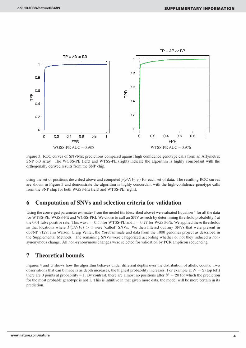
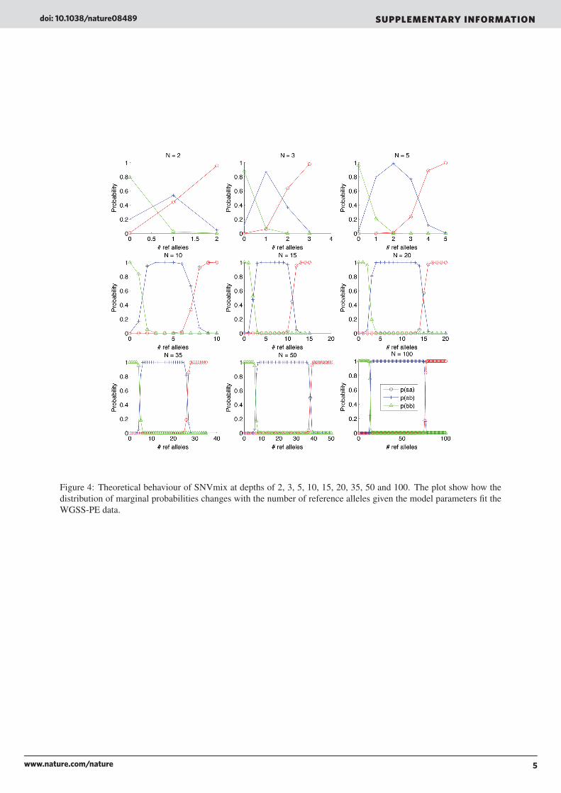
7 Theoretical boundsFigures 4 and 5 shows how the algorithm behaves under different depths over the distribution of allelic counts. Twoobservations that can b made is as depth increases, the highest probability increases. For example at N = 2 (top left)there are 0 points at probability = 1. By contrast, there are almost no positions after N = 20 for which the predictionfor the most probable genotype is not 1. This is intuitive in that given more data, the model will be more certain in itsprediction.

4



Figure 4: Theoretical behaviour of SNVmix at depths of 2, 3, 5, 10, 15, 20, 35, 50 and 100. The plot show how thedistribution of marginal probabilities changes with the number of reference alleles given the model parameters fit theWGSS-PE data.

5



Figure 5: Theoretical behaviour of SNVmix at depths of 2, 3, 5, 10, 15, 20, 35, 50 and 100. The plot show how thedistribution of marginal probabilities changes with the number of reference alleles given the model parameters fit theWTSS-PE data.

6



References[1] Christopher M. Bishop. Pattern Recognition and Machine Learning (Information Science and Statistics). Springer,

August 2006.

[2] B Carvalho, H Bengtsson, T P Speed, and R A Irizarry. Exploration, normalization, and genotype calls of high-density oligonucleotide snp array data. Biostatistics, 8(2):485–499, Apr 2007.

7

Documents

Supplemental Appendix 1 - inferring SNVs from … · Supplemental Appendix 1 - inferring SNVs from aligned reads using a Bayesian mixture model Sohrab P. Shah, Ryan D. Morin and Samuel