Embed Size (px)
Citation preview
CRANFIELD UNIVERSITY
Xiaoheng Jiang
The impact of process variables and wear characteristics on
the cutting tool performance using Finite Element Analysis
SCHOOL OF AEROSPACE TRANSPORT AND
MANUFACTURING
MSc by research
Academic Year 2015 - 2016
Supervisors Dr Konstantinos Salonitis amp Dr Sue
Impey
SEPTEMBER 2016
CRANFIELD UNIVERSITY
SCHOOL OF AEROSPACE TRANSPORT AND
MANUFACTURING
MSc by research
Academic Year 2015 - 2016
Xiaoheng Jiang
The impact of process variables and wear characteristics on
the cutting tool performance using Finite Element Analysis
Supervisors Dr Konstantinos Salonitis amp Dr Sue
Impey
SEPTEMBER 2016
copy Cranfield University 2016 All rights reserved No part of
this publication may be reproduced without the written
permission of the copyright owner
i
ABSTRACT
The frequent failure of cutting tool in the cutting process may cause a
huge loss of money and time especially for hard to machine materials such
as titanium alloys Thus this study is mainly focused on the impact of wear
characteristics and process variables on the cutting tool which is ignored by
most of researchers A thermo-mechanical finite element model of orthogonal
metal cutting with segment chip formation is presented This model can be
used to predict the process performance in the form of cutting force
temperature distribution and stress distribution as a function of process
parameters Ls-dyna is adopted as the finite element package due to its
ability in solving dynamic problems Ti-6Al-4V is the workpiece material due
to its excellent physical property and very hard to machine This thesis uses
the Johnson-Cook constitutive model to represent the flow stress of
workpiece material and the Johnson-Cook damage model to simulate the
failure of the workpiece elements The impacts of process variables and tool
wear are investigated through changing the value of the variables and tool
geometry
It is found that flank wear length has a linear relationship with the cutting
force which is useful for predicting the cutting tool performance Increasing
the crater wear will in some degree diminishes the cutting force and
temperature A chip breakage will also happen in some cases of crater wear
Through these findings the relationship between flank wear and cutting
power is established which can be used as the guidance in the workshop for
changing the tools The distribution of temperature and stress on the cutting
tool in different cutting conditions can be adopted to predict the most possible
position forming cutting tool wear
Keywords FEM cutting temperature Ls-dyna Ti-6Al-4V flank wear
crater wear cutting power
ii
ACKNOWLEDGEMENTS
I would like to express my deep sense of gratitude to Dr Konstantinos
Salonitis and Dr Sue Impey for their excellent supervision and patience during
my research process in Cranfield University They teach me a lot of methods
needed for doing a research project It is more important than specific
knowledge and will benefit me for a life time
I am very much thankful to Dr Jorn Mehnen and Dr Chris Sansom for
their genius suggestions in my review processes Their ideas are essential
for my research process and the final thesis writing
I also thank Mr Ben Labo the employee of Livermore Software
Technology Corp (LSTC) with his help on the Ls-dyna the simulation
process becomes much easier
It is my privilege to thank my wife Mrs Yongyu Wang and my parents for
their love and constant encouragement throughout my research period
Finally I would like to give my sincere thanks to my company the
Commercial Aircraft Corporation of China Ltd and China Scholarship
Council for having sponsored and supported my stay in Cranfield University
iii
TABLE OF CONTENTS
ABSTRACT i
ACKNOWLEDGEMENTS ii
TABLE OF CONTENTS iii
LIST OF FIGURES vii
LIST OF TABLES xii
LIST OF ABBREVIATIONS xiii
1 Introduction 1
11 The background of the research 1
12 Aim and objectives of the research 3
13 Research methodology 3
2 Literature review 6
21 The tool wear types and tool wear mechanisms 6
22 The elements influencing tool wear 10
23 Tool life and wear evolution models 13
24 Analytical models 16
241 Shear plane models 16
242 Slip-line models 19
25 Finite element method 23
26 Key findings and research gap 25
3 Finite element simulation of metal cutting 26
31 Introduction 26
32 The selection of finite element package 27
321 Explicit and implicit 27
3211 Explicit and implicit solution method 27
3212 Iterative scheme 29
3213 Choice in cutting process 30
322 Description of motion 30
323 Selection of Finite element package 32
33 Workpiece material and different models for modelling 36
331 The chosen of workpiece material 36
332 The workpiece constitutive model 39
iv
3321 The JohnsonndashCook (J-C) model 40
3322 The SteinbergndashCochranndashGuinanndashLund (SCGL) model 40
3323 The ZerillindashArmstrong (Z-A) model 42
3324 Evaluation of three models 43
333 The workpiece damage model 44
3331 Damage initiation 44
3332 Damage evolution 45
34 Chip formation process 47
341 Introduction 47
342 Chip formation mechanism 47
3421 Continuous Chips 48
3422 Lamellar Chips 50
3423 Segment Chips 51
3424 Discontinuous Chips 52
3425 Experiments to understand the chip-formation process 52
343 Chip separation criteria 53
3431 Geometrical method 54
3432 Physical method 55
344 Friction model 56
3441 Constant Coulomb (model I) 56
3442 Constant Shear (model II) 57
3443 Constant Shear in Sticking Zone and Constant Coulomb
in Sliding Zone (model III) 57
3444 Choice in the thesis 59
35 Summary 59
4 Modelling and simulation 60
41 Introduction 60
42 Assumptions for modelling 60
43 Cutting tool modelling 61
44 Workpiece modelling 62
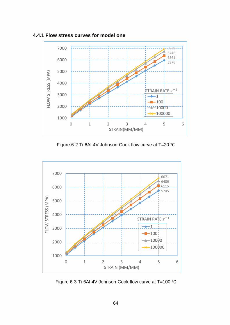
441 Flow stress curves for model one 64
442 Flow stress curves for model two 67
v
443 Difference between two constitutive models 70
4431 Effect of strain rate 70
4432 Effect of strain 70
4433 Effect of temperature 71
45 System modelling 73
46 Parameters adopted in the cutting process 74
461 Validation model 75
462 Effects of different cutting parameters 75
463 Effects of different wear types 75
5 Model validation 78
6 Results and discussion 81
61 Effects of different process parameters on cutting tool 81
611 The effects of cutting speed 81
6111 The effect of cutting speed on the cutting force 81
6112 The effect of cutting speed on the cutting tool maximum
temperature 83
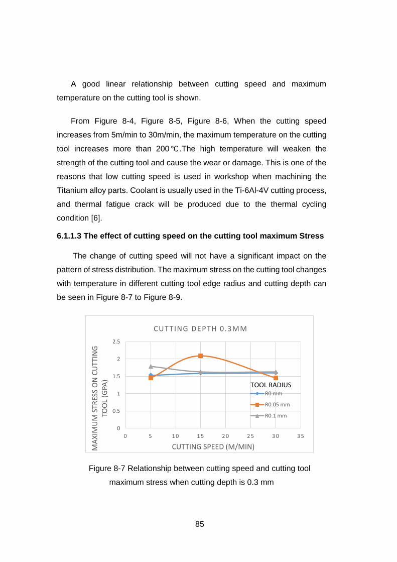
6113 The effect of cutting speed on the cutting tool maximum
Stress 85
612 The effects of cutting depth 87
6121 The effect of cutting depth on the cutting force 87
6122 The effect of cutting depth on the cutting tool maximum
temperature 89
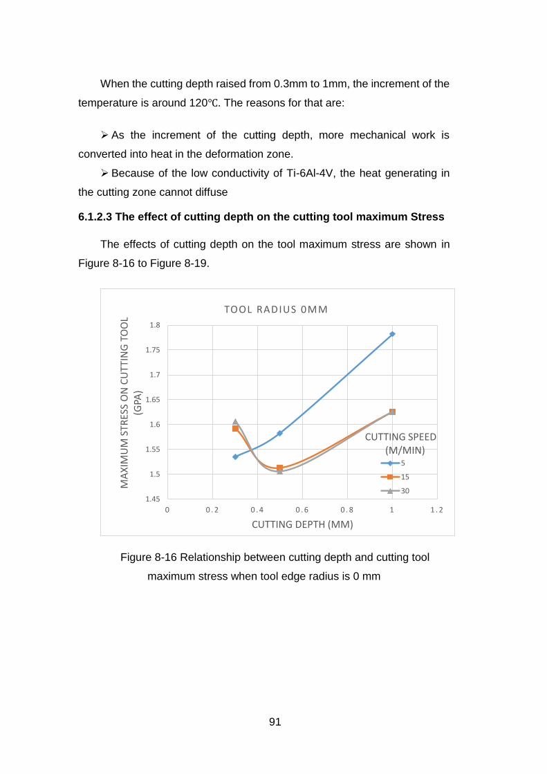
6123 The effect of cutting depth on the cutting tool maximum
Stress 91
613 The effects of tool edge radius 93
6131 The effect of cutting tool edge radius on the cutting force 93
6132 The effect of cutting tool edge radius on the cutting tool
maximum temperature 95
6133 The effect of cutting tool edge radius on the cutting tool
maximum Stress 98
62 The effects of flank wear 100
621 The effect of flank wear on the cutting force 101
vi
622 The effect of flank wear on the cutting tool temperature
distribution 102
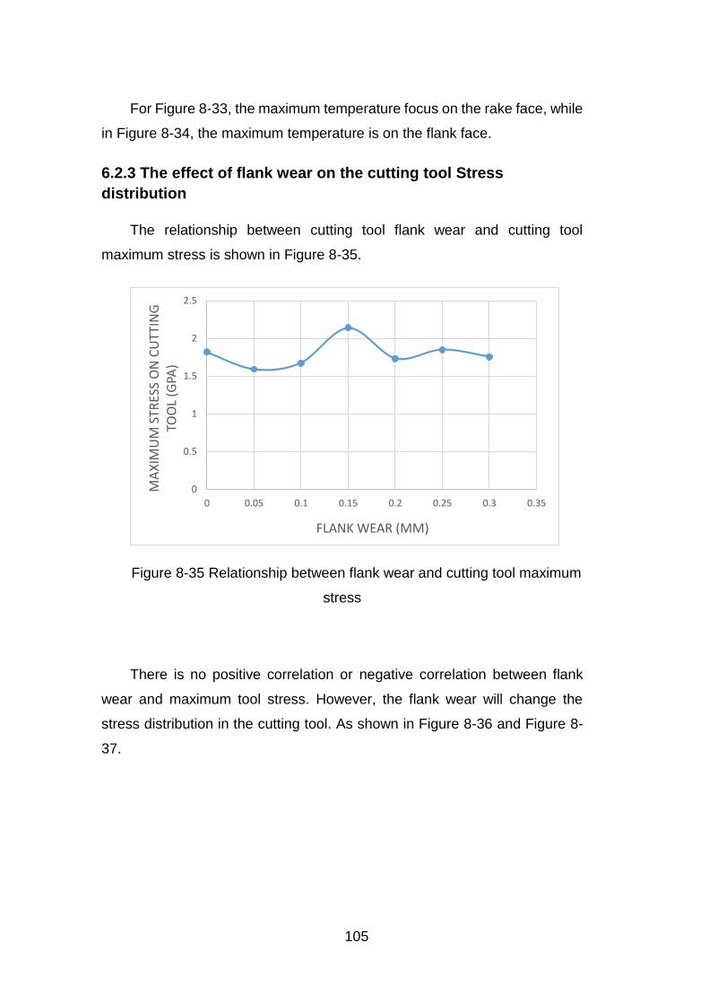
623 The effect of flank wear on the cutting tool Stress distribution 105
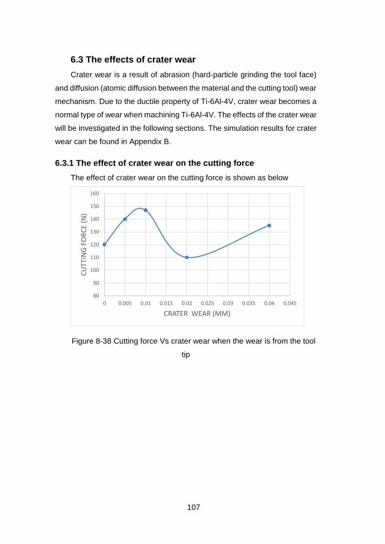
63 The effects of crater wear 107
631 The effect of crater wear on the cutting force 107
632 The effect of crater wear on the cutting tool temperature
distribution 109
633 The effect of crater wear on the cutting tool Stress distribution
111
64 Limitation of the work 113
7 Conclusions and Future work 114
71 Conclusions 114
72 Future work 115
REFERENCES 117
APPENDICES 130
Appendix A Simulation results for different process parameters 130
Appendix B Simulation results for different tool wear 135
vii
LIST OF FIGURES
Figure 2-1 Flank wear and crater wear [7] 7
Figure 2-2 Tool wear evolution [8] 8
Figure 2-3 Tool wear mechanism for different wear types [3] 9
Figure 2-4 Four major elements influencing tool wear in machining process
[10] 10
Figure 2-5 Properties of cutting tool materials [16] 12
Figure 2-6 Methodology for cutting tool selection [16] 12
Figure 2-7 Merchantrsquos circle [28] 17
Figure 2-8 Lee and Shafferrsquos slip-line theory for orthogonal cutting [29] 20
Figure 2-9 Fangrsquos model [30] 21
Figure 2-10 Eight special cases of new slip-line model [30] 22
Figure 5-1 Explicit time scheme (every time distance is ∆1199052) 28
Figure 5-2 Newton-Raphson iterative method 29
Figure 5-3 One dimensional example of lagrangian Eulerian and ALE mesh
and particle motion [67] 31
Figure 5-4 The usage ratio of different finite element packages [70] 32
Figure 5-5 Temperature distribution when flank wear inclination=12degwear
land=2mm [72] 33
Figure 5-6 Maximum shear stress in the tool and workpiece [42] 34
Figure 5-7 Temperature distribution on cutting tool workpiece and chip [46] 35
Figure 5-8 Von Mises stress field for tool with different rake angle a) -5 degb) 0 deg
c) 5 degd) 10 deg [73] 36
Figure 5-9 The weight ratio for different materials in Boeing 777 [75] 38
Figure 5-10 The weight ratio for different materials in Boeing 787 [76] 39
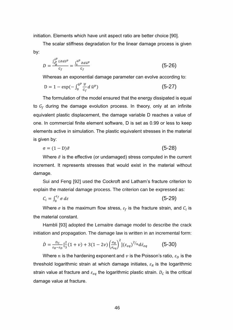
Figure 5-11 Typical uniaxial stress-strain in case of a ductile metal [90] 44
Figure 5-12 Four types of chips [94] 48
Figure 5-13 Flow stress property 49
Figure 5-14 Continue chip formation 49
Figure 5-15 Condition for lamellar chip 51
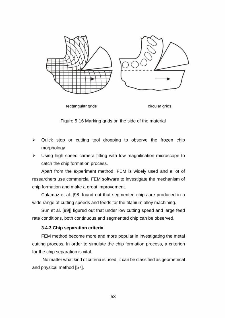
Figure 5-16 Marking grids on the side of the material 53
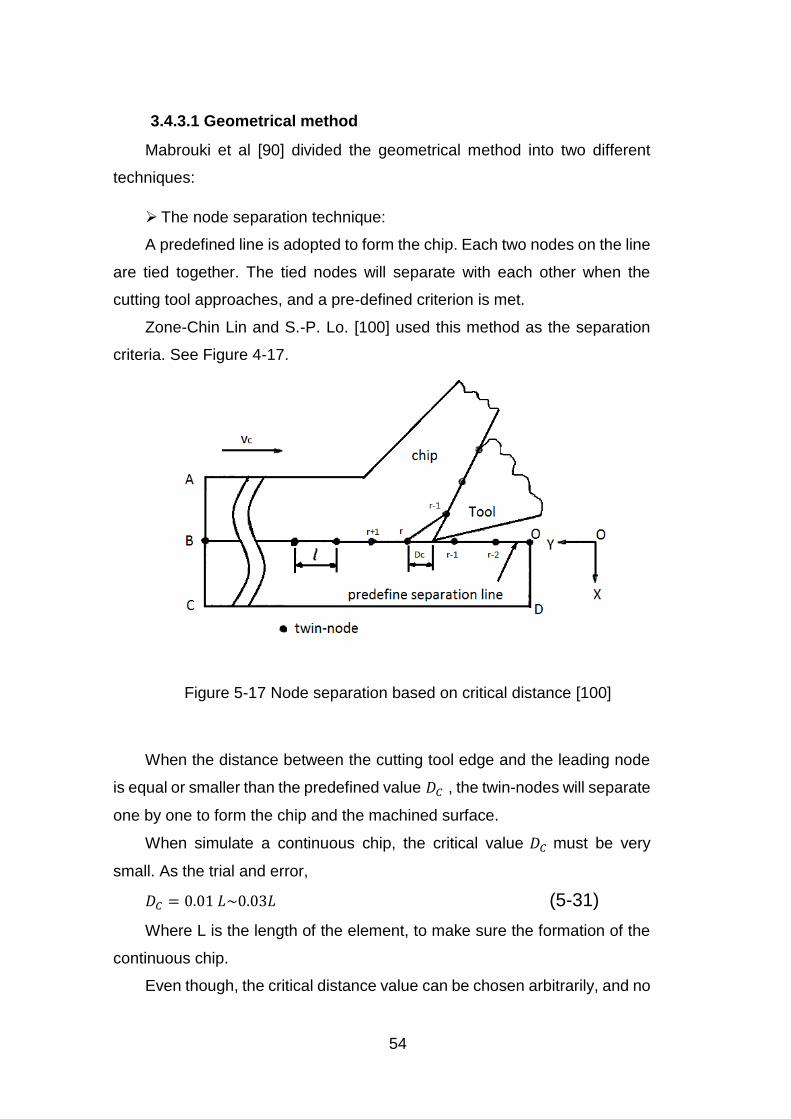
Figure 5-17 Node separation based on critical distance [100] 54
viii
Figure 5-18 Physical separation criteria [57] 56
Figure 5-19 Distribution of normal and shear stress on the rake face 58
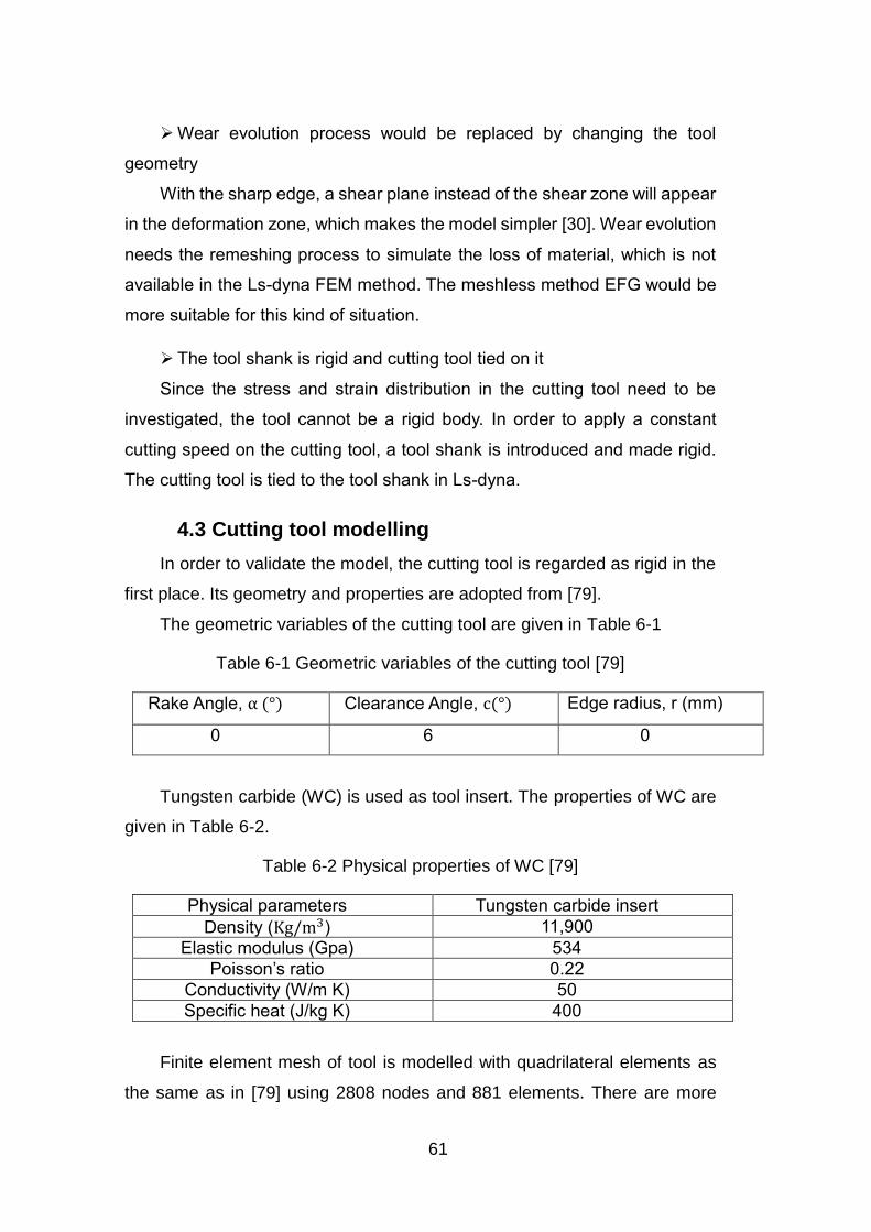
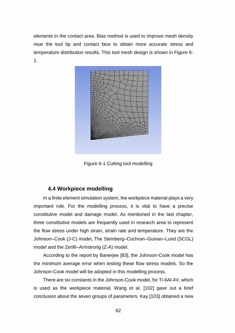
Figure 6-1 Cutting tool modelling 62
Figure6-2 Ti-6Al-4V Johnson-Cook flow curve at T=20 64
Figure 6-3 Ti-6Al-4V Johnson-Cook flow curve at T=100 64
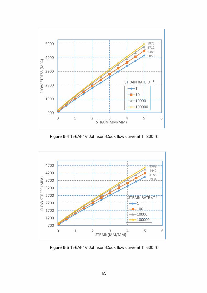
Figure 6-4 Ti-6Al-4V Johnson-Cook flow curve at T=300 65
Figure 6-5 Ti-6Al-4V Johnson-Cook flow curve at T=600 65
Figure 6-6 Ti-6Al-4V Johnson-Cook flow curve at T=900 66
Figure 6-7 Ti-6Al-4V Johnson-Cook flow curve at T=1200 66
Figure 6-8 Ti-6Al-4V Johnson-Cook flow curve at T=20 67
Figure 6-9 Ti-6Al-4V Johnson-Cook flow curve at T=100 67
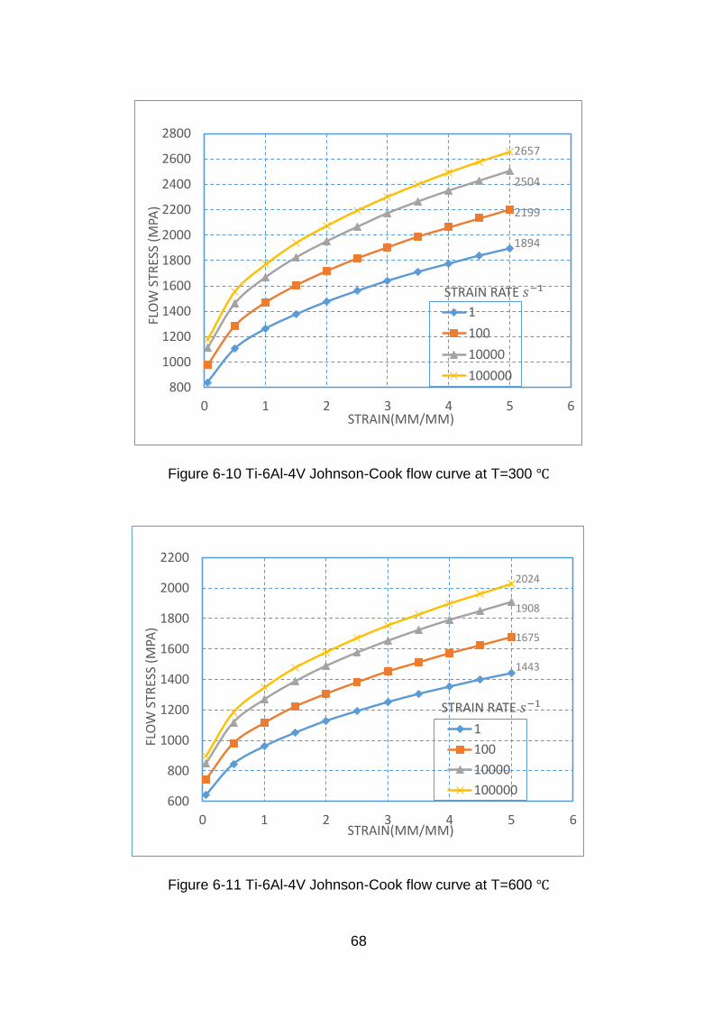
Figure 6-10 Ti-6Al-4V Johnson-Cook flow curve at T=300 68
Figure 6-11 Ti-6Al-4V Johnson-Cook flow curve at T=600 68
Figure 6-12 Ti-6Al-4V Johnson-Cook flow curve at T=900 69
Figure 6-13 Ti-6Al-4V Johnson-Cook flow curve at T=1200 69
Figure 6-14 The effect of strain rate 70
Figure 6-15 The effect of strain 71
Figure 6-16 The effect of temperature 71
Figure 6-17 The workpiece modelling 73
Figure 6-18 Cutting system 73
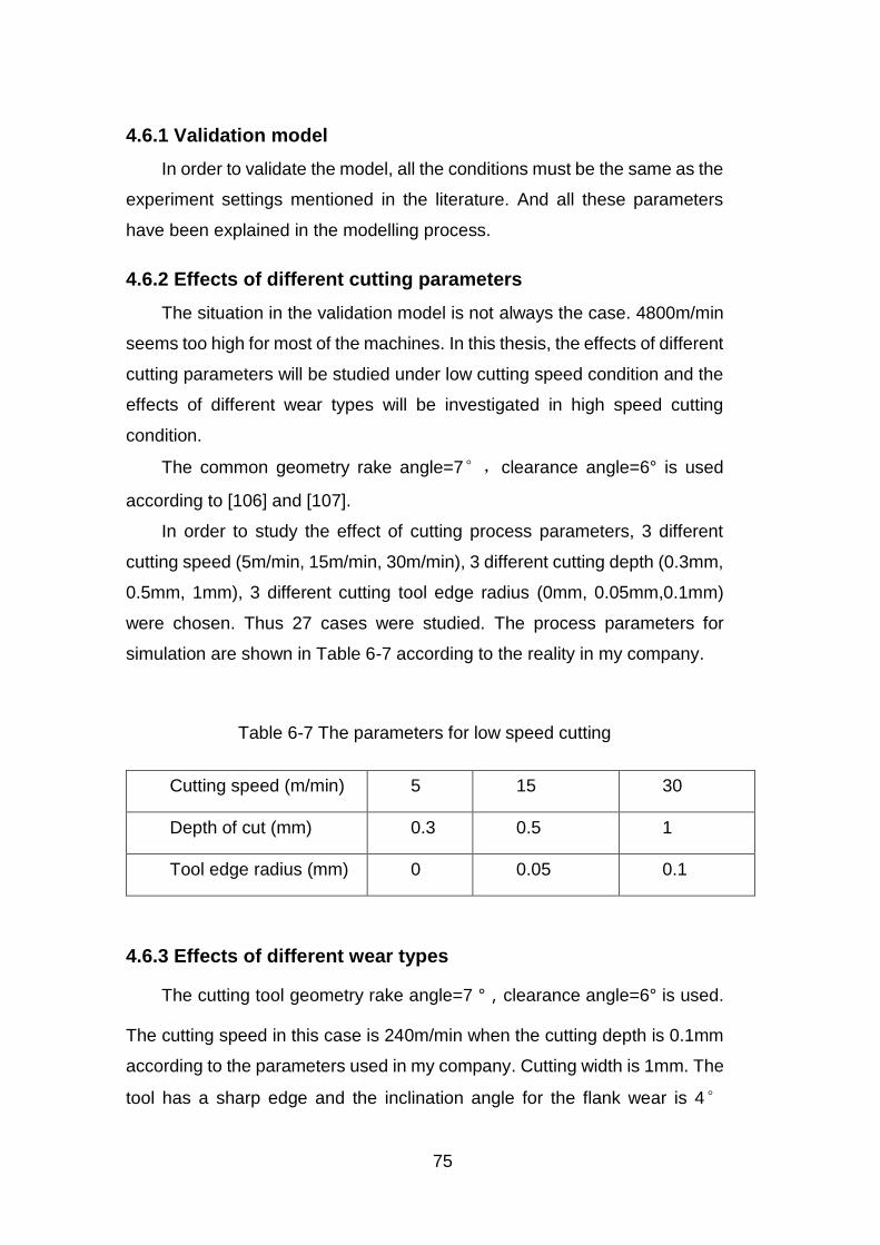
Figure 6-19 Flank wear land 76
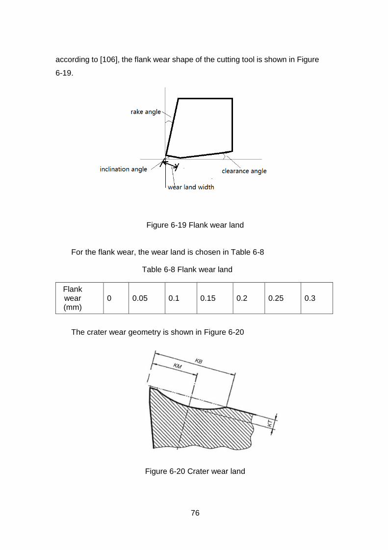
Figure 6-20 Crater wear land 76
Figure 7-1 Chip formation for model one 78
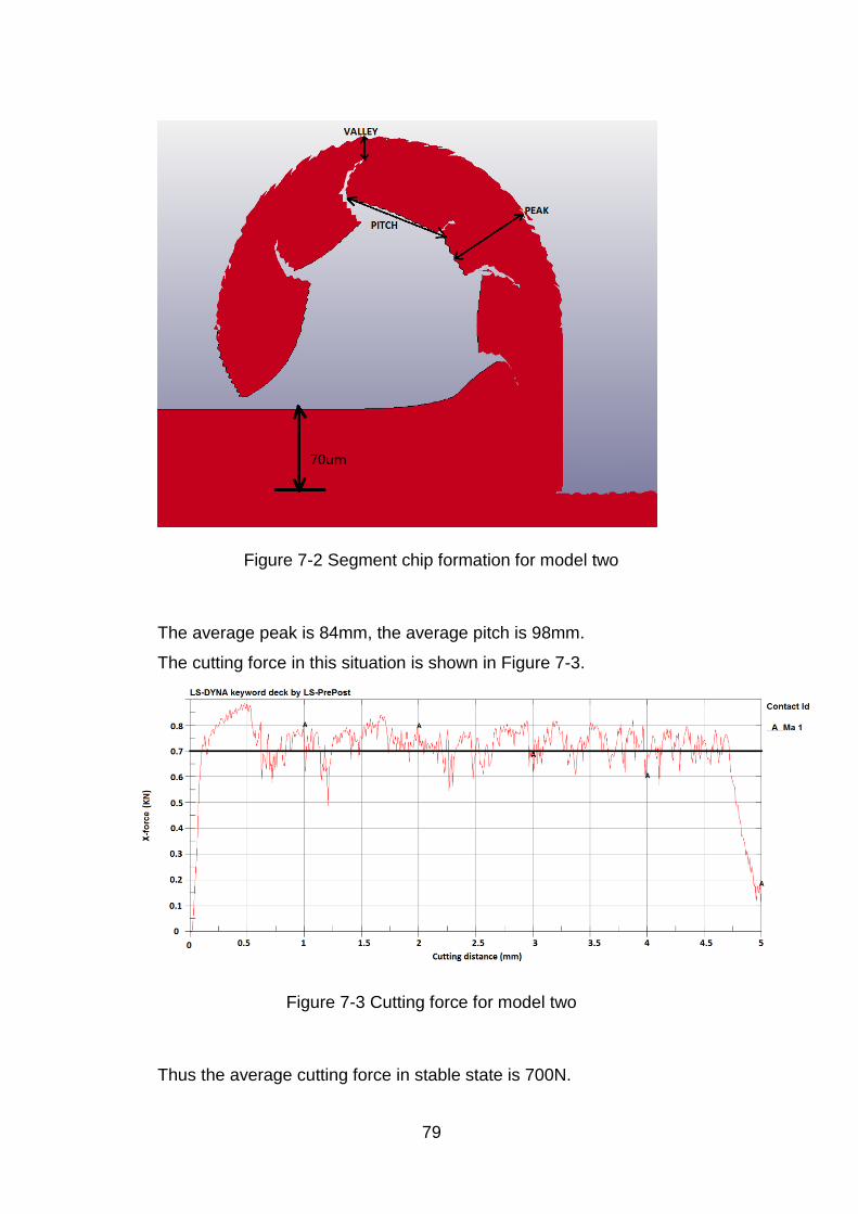
Figure 7-2 Segment chip formation for model two 79
Figure 7-3 Cutting force for model two 79
Figure 8-1 Relationship between cutting speed and cutting force when cutting
depth is 03mm 81
Figure 8-2 Relationship between cutting speed and cutting force when cutting
depth is 05mm 82
Figure 8-3 Relationship between cutting speed and cutting force when cutting
depth is 1mm 82
ix
Figure 8-4 Relationship between cutting speed and cutting tool maximum
temperature when cutting depth is 03 mm 83
Figure 8-5 Relationship between cutting speed and cutting tool maximum
temperature when cutting depth is 05 mm 84
Figure 8-6 Relationship between cutting speed and cutting tool maximum
temperature when cutting depth is 1 mm 84
Figure 8-7 Relationship between cutting speed and cutting tool maximum
stress when cutting depth is 03 mm 85
Figure 8-8 Relationship between cutting speed and cutting tool maximum
stress when cutting depth is 05 mm 86
Figure 8-9 Relationship between cutting speed and cutting tool maximum
stress when cutting depth is 1 mm 86
Figure 8-10 Relationship between cutting depth and cutting force when tool
edge radius is 0 mm 87
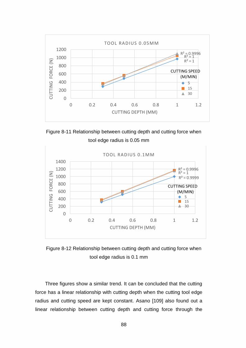
Figure 8-11 Relationship between cutting depth and cutting force when tool
edge radius is 005 mm 88
Figure 8-12 Relationship between cutting depth and cutting force when tool
edge radius is 01 mm 88
Figure 8-13 Relationship between cutting depth and cutting tool maximum
temperature when tool edge radius is 0 mm 89
Figure 8-14 Relationship between cutting depth and cutting tool maximum
temperature when tool edge radius is 005 mm 90
Figure 8-15 Relationship between cutting depth and cutting tool maximum
temperature when tool edge radius is 01 mm 90
Figure 8-16 Relationship between cutting depth and cutting tool maximum
stress when tool edge radius is 0 mm 91
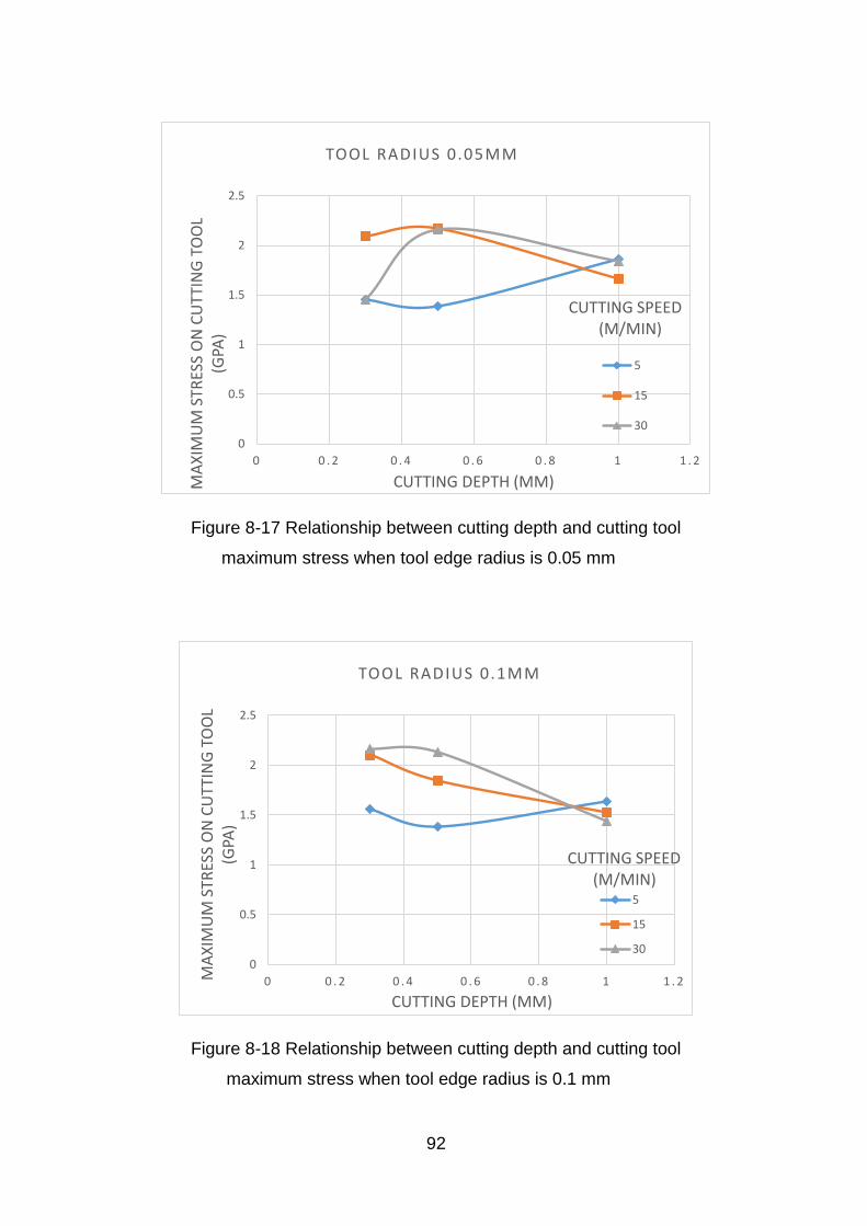
Figure 8-17 Relationship between cutting depth and cutting tool maximum
stress when tool edge radius is 005 mm 92
Figure 8-18 Relationship between cutting depth and cutting tool maximum
stress when tool edge radius is 01 mm 92
Figure 8-19 Relationship between cutting tool edge radius and cutting force
when cutting depth is 03 mm 93
x
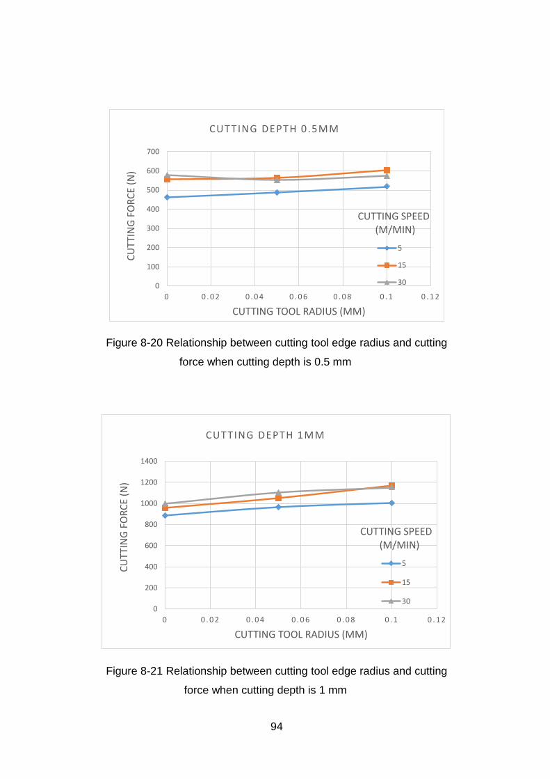
Figure 8-20 Relationship between cutting tool edge radius and cutting force
when cutting depth is 05 mm 94
Figure 8-21 Relationship between cutting tool edge radius and cutting force
when cutting depth is 1 mm 94
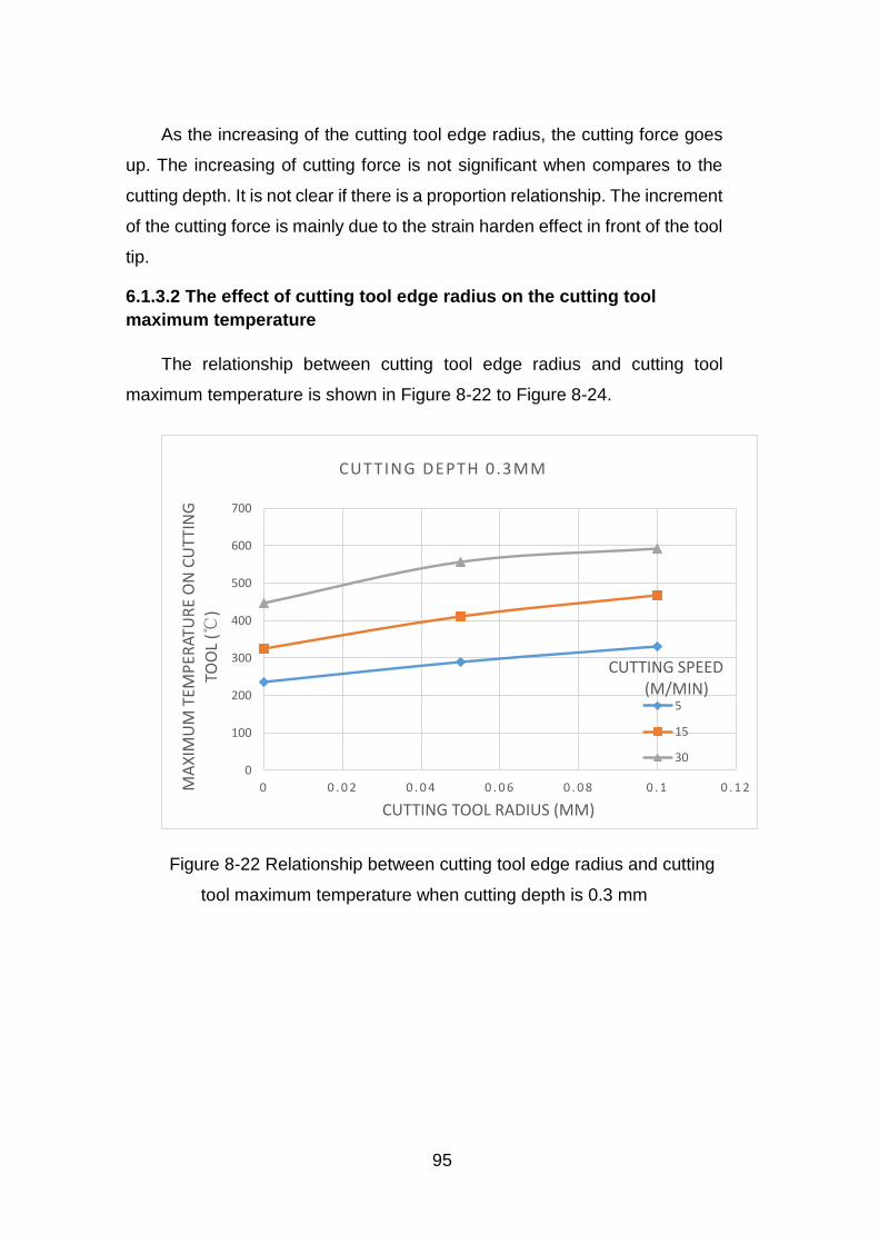
Figure 8-22 Relationship between cutting tool edge radius and cutting tool
maximum temperature when cutting depth is 03 mm 95
Figure 8-23 Relationship between cutting tool edge radius and cutting tool
maximum temperature when cutting depth is 05 mm 96
Figure 8-24 Relationship between cutting tool edge radius and cutting tool
maximum temperature when cutting depth is 1mm 96
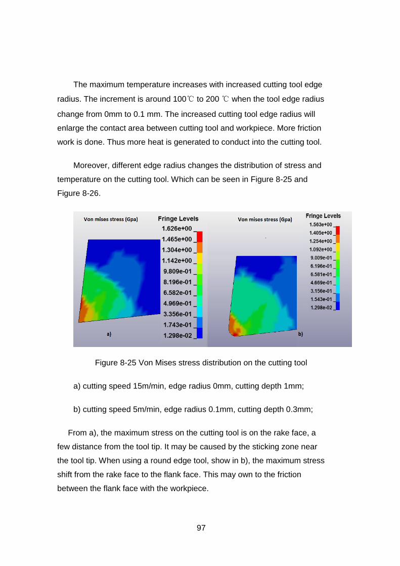
Figure 8-25 Von Mises stress distribution on the cutting tool 97
Figure 8-26 Temperature distribution on the cutting tool 98
Figure 8-27 Relationship between cutting tool edge radius and cutting tool
maximum stress when cutting depth is 03 mm 99
Figure 8-28 Relationship between cutting tool edge radius and cutting tool
maximum stress when cutting depth is 05 mm 99
Figure 8-29 Relationship between cutting tool edge radius and cutting tool
maximum stress when cutting depth is 1 mm 100
Figure 8-30 The relationship between flank wear and cutting force 101
Figure 8-31 The relationship between flank wear and machining power 102
Figure 8-32 The relationship between cutting tool flank wear and cutting tool
maximum temperature 103
Figure 8-33 Temperature distribution with a new tool 104
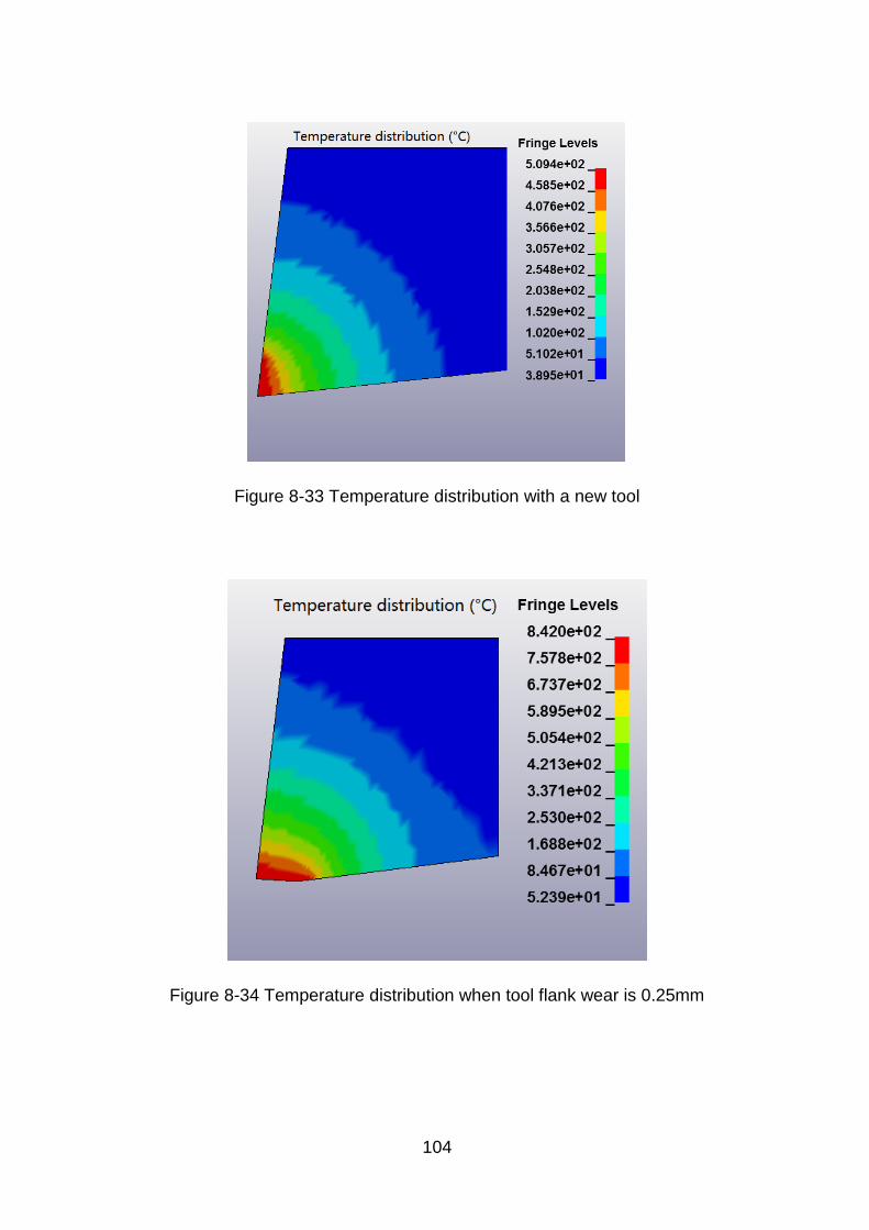
Figure 8-34 Temperature distribution when tool flank wear is 025mm 104
Figure 8-35 Relationship between flank wear and cutting tool maximum
stress 105
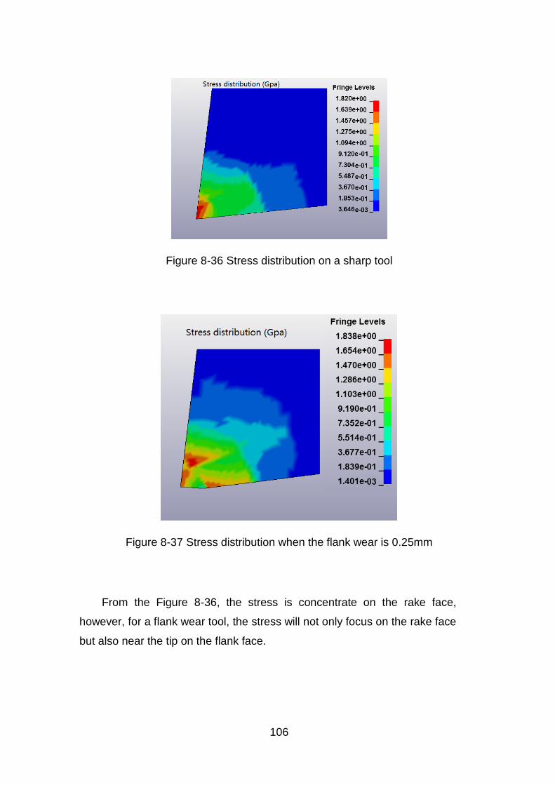
Figure 8-36 Stress distribution on a sharp tool 106
Figure 8-37 Stress distribution when the flank wear is 025mm 106
Figure 8-38 Cutting force Vs crater wear when the wear is from the tool tip 107
Figure 8-39 Cutting force Vs crater wear when the wear is 10 μm from the
tool tip 108
Figure 8-40 Chip breakage 109
xi
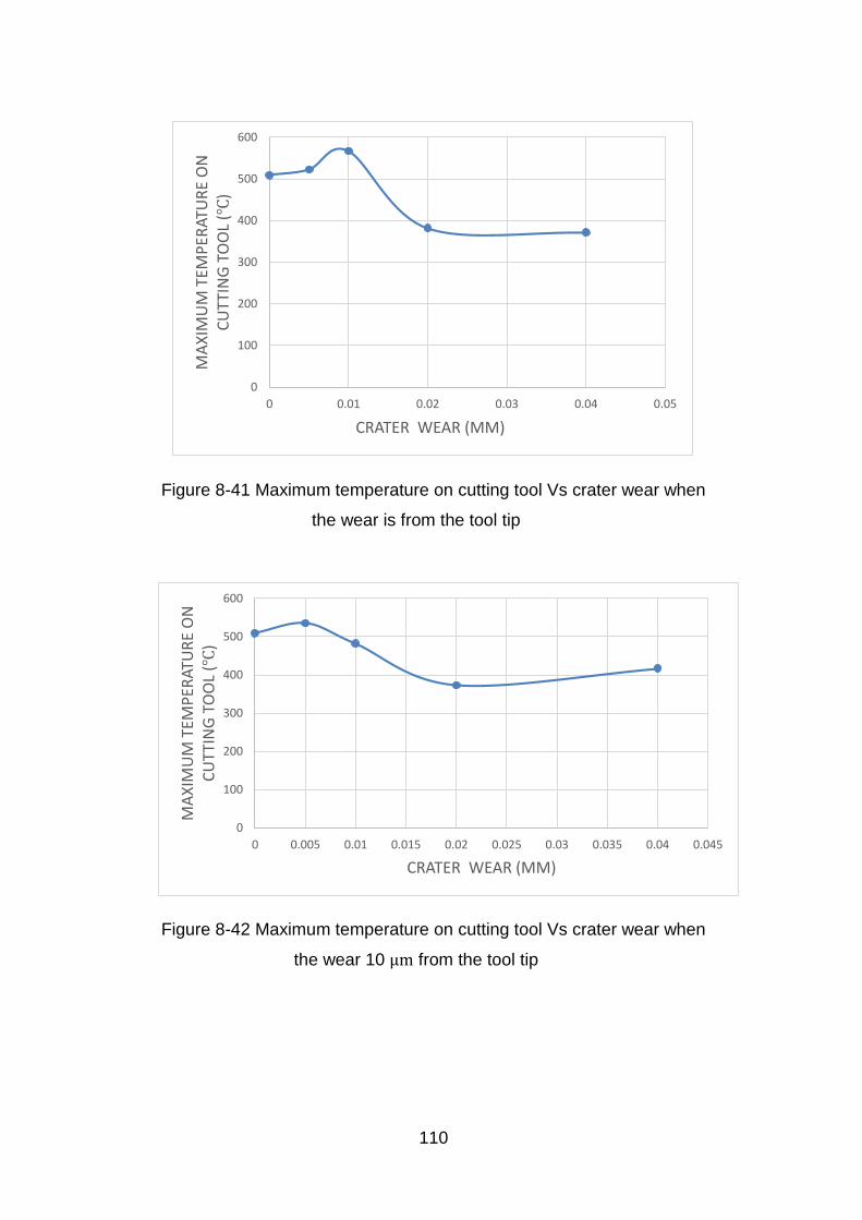
Figure 8-41 Maximum temperature on cutting tool Vs crater wear when the
wear is from the tool tip 110
Figure 8-42 Maximum temperature on cutting tool Vs crater wear when the
wear 10 μm from the tool tip 110
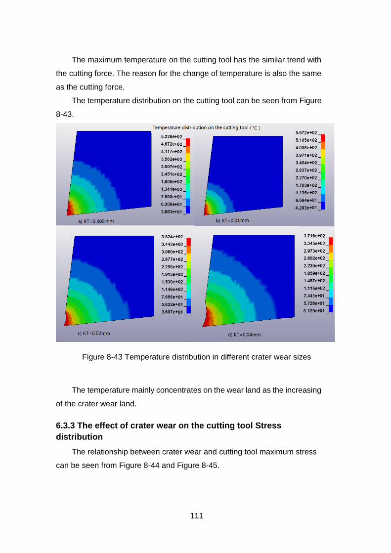
Figure 8-43 Temperature distribution in different crater wear sizes 111
Figure 8-44 Maximum stress on cutting tool Vs crater wear when the wear is
from the tool tip 112
Figure 8-45 Maximum stress on cutting tool Vs crater wear when the wear 10
μm from the tool tip 112
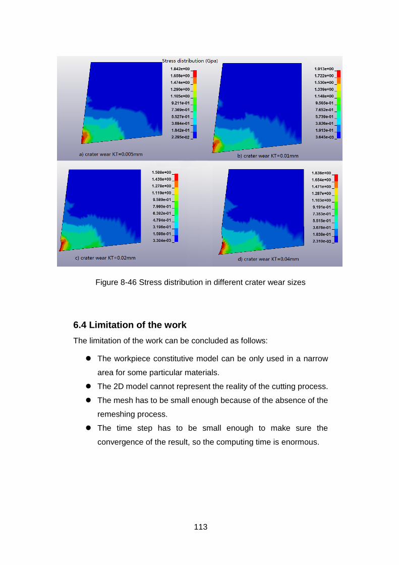
Figure 8-46 Stress distribution in different crater wear sizes 113
xii
LIST OF TABLES
Table 2-1 Tool wear rate models 15
Table 5-1 The physical property of three different alloys [74] 37
Table 5-2 The machining easiness of different alloys [77] 39
Table 5-3 Average maximum absolute errors [83] 43
Table 6-1 Geometric variables of the cutting tool [79] 61
Table 6-2 Physical properties of WC [79] 61
Table 6-3 Johnson-Cook constants 63
Table 6-4 Johnson-Cook damage model constants for Ti-6Al-4V [79] 72
Table 6-5 Physical properties of Ti-6Al-4V [79] 72
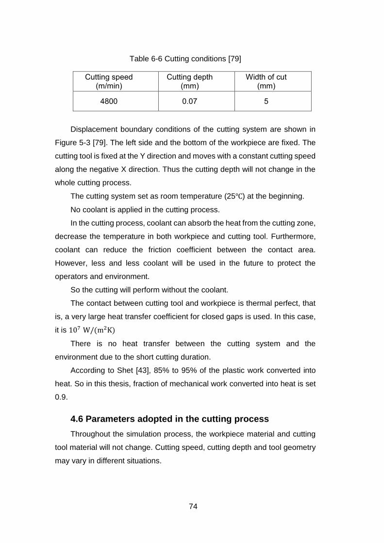
Table 6-6 Cutting conditions [79] 74
Table 6-7 The parameters for low speed cutting 75
Table 6-8 Flank wear land 76
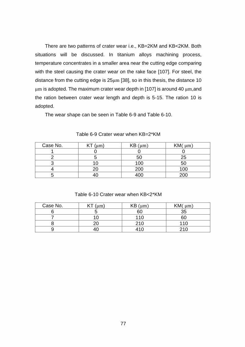
Table 6-9 Crater wear when KB=2KM 77
Table 6-10 Crater wear when KBlt2KM 77
Table 7-1 Comparison of predicted chip morphology with experiment data 80
Table 7-2 Comparison of predicted cutting force with experiment data 80
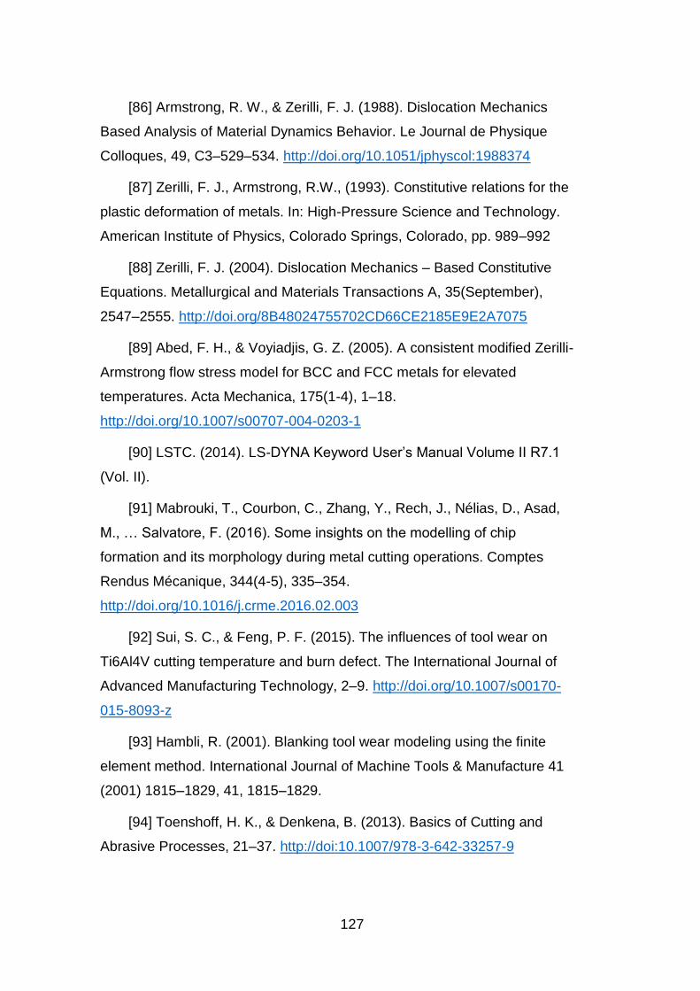
Table A-1 Simulation results using the sharp tool and 03mm cutting depth 130
Table A-2 Simulation results using the sharp tool and 05mm cutting depth 130
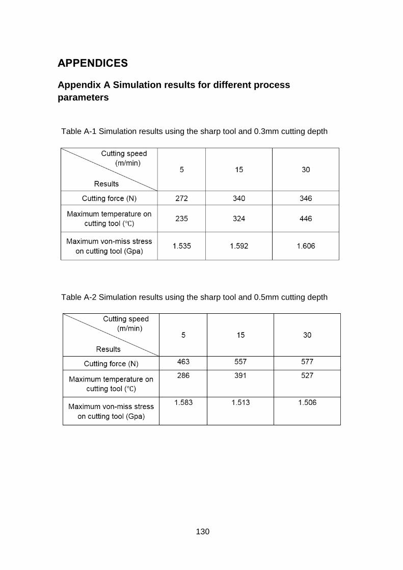
Table A-3 Simulation results using the sharp tool and 1mm cutting depth 131
Table A-4 Simulation results using the R005 tool and 03mm cutting depth 131
Table A-5 Simulation results using the R005 tool and 05mm cutting depth 132
Table A-6 Simulation results using the R005 tool and 1mm cutting depth 132
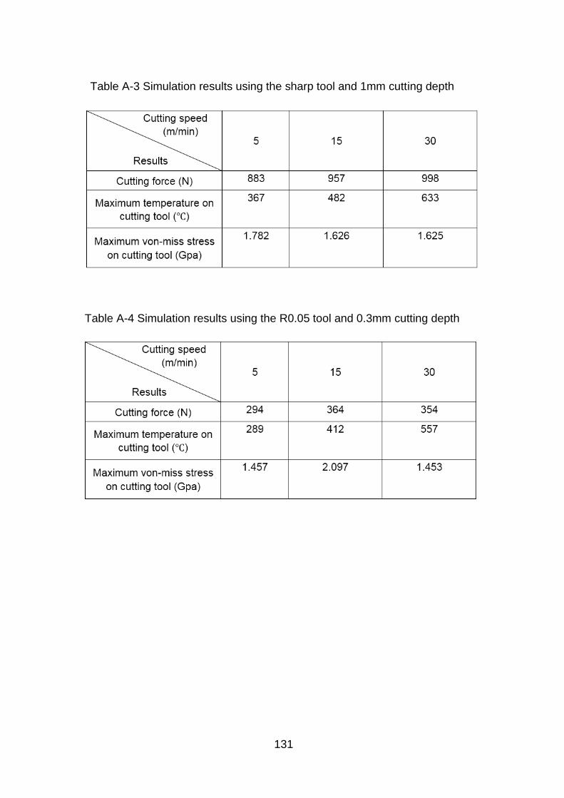
Table A-7 Simulation results using the R01 tool and 03mm cutting depth 133
Table A-8 Simulation results using the R01 tool and 05mm cutting depth 133
Table A-9 Simulation results using the R01 tool and 1mm cutting depth 134
Table B-1 Simulation results for flank wear 135
Table B-2 Simulation results when crater wear is 10 μm from tool tip 135
Table B-3 Simulation results when crater wear is from tool tip 135
xiii
LIST OF ABBREVIATIONS
ALE Arbitrary LagrangianndashEulerian
BUE Build-up edge
DOE Design of experiments
FEA Finite Element Analysis
FEM Finite Element Method
RSM Response surface methodology
1
1 Introduction
11 The background of the research
Since the development of the CNC machining technology metal cutting
industry has become a significant sector both in the developed and
developing countries It is not only widely used in high technology industries
such as automotive engine robot and aerospace but also in some ordinary
products such as the gears in the bicycle Rhodes [1] mentioned that the
manufacturing industry accounted for 10 or pound1507 billion economic output
of UK and employed around 26 million people in 2013 Metal cutting sector
was about 11 of the total manufacturing industry Jablonowski and Eigel-
Miller [2] pointed out that in 2012 the machine-tool output value by 28
principal producing countries in the world was $943 billion Thus it is vital to
investigate the metal cutting process to create more value for the society
The metal cutting process is usually consisted of cutting machine fixture
tool holder cutting tool and workpiece Generally the cutting machine fixture
and tool holder can be used for a long time and still have acceptable
accuracy For cutting tool the failure of it may not only lead to the rejection
of the final part and waste of the time waiting for the tool to be discarded or
repaired but also cause the break down of the expensive cutting machine
even interrupting the whole production line Thus the cutting tool has to be
replaced before the end of its life in order to get the designed dimensional
accuracy and surface finishing since the happening of cutting tool wear in the
cutting process Salonitis amp Kolios [3] mentioned that only 50ndash80 of the
expected tool life is typically used according to [4]
Thus it is very important to understand metal cutting process including
the types of cutting tool wear the causes of tool wear and the mechanisms
behind them After that the impacts of various cutting parameters and the
cutting tool wear on the cutting tool should be investigated
Many methods can be applied to study the impacts of various cutting
parameters and the cutting tool wear
People acquire some results from the experiments in the first place
These are very helpful to understand the whole cutting process However
2
experiments can be very expensive and time consuming especially for
machining process Workpiece material may be damaged the machine is
occupied people have to spend a lot of time observing the process and
recording the data The most frustrating thing is that when a small cutting
condition (such as cutting speed) is changed the experimentrsquos results cannot
be adopted anymore
Modelling of the cutting process is another way to investigate the metal
cutting Markopoulos [5] introduced the brief history of the developing of
modelling methods In the original thoughts researchers were trying to use
theoretic and modelling methods to estimate the performance of the cutting
process and find out solutions for realistic problems in the workshop without
any experimental work Around 1900s simplified analytical models started
publishing In 1950s modelling methods took the leading place for
understanding machining mechanism and investigating the cutting process
In the early 1970s papers using Finite Element Method (FEM) on machining
process modelling began to publish in scientific journals Through the
development of computing ability and commercial FEM software FEM
method has become the favourite modelling tool for researchers in the cutting
area By using the finite element methods basic knowledge about the
machining mechanisms is acquired Researchers can learn the process
parameters such as temperature strain stress cutting force from the model
and predict the quality of the product conveniently
In this thesis an orthogonal metal cutting model is established using
finite element method In chapter two literature review will be carried out to
understand the previous work and find out the research gap for the thesis In
chapter three aims and objectives will be emphasized Research
methodology will be explained in the following chapter Fundamental
knowledge for modelling metal cutting process are presented in chapter five
In chapter six present cutting model is explained Model validation will be
carried out in chapter seven Results and discussion are presented in chapter
eight In the final chapter the conclusion of the study is given
3
12 Aim and objectives of the research
Due to the importance of the cutting tool in the machining process and
the absence of papers on the impacts of process variables and wear
characteristics on the cutting tool the aim of the present thesis will be
Investigating the impacts that various process parameters and tool wear
characteristics have on the cutting tool and link the wear evolution with
measurable machine tool metrics
The objectives of the research are to
1 Develop a cutting model using commercial FE package
to predict the cutting process variables (such as cutting
temperature forces etc)
2 Validate the FE model using experiment results from the
published literatures
3 Predict the effects of cutting speed depth tool edge
radius and wear geometry on the cutting force stress and
temperature distribution mainly on cutting tool
4 Establish the relationship between flank wear and
machine power in order to predict a critical spindle power value
for changing the cutting tool
13 Research methodology
The research process will follow 5 phases which is shown in Figure 1-1
4
Figure 1-1 Research methodology
In the phase 1 literature review will be done mainly about the software
the material model and the tool wear background information In this phase
the most important thing is to get a general idea about the research gap
aims objectives and way to finish this project
5
In the phase 2 tool wear model will be built through the commercial finite
element software Ls-dyna In this progress material model structure
meshing remeshing process code development and separation criterial are
needed to be considered Some assumption will be made in this phase in
order to simplify the model But the most important thing is to make sure the
accuracy of this simplified model The model has to be validated through
some experiments or tests done by other papers by comparing the simulation
results So the modelling process may be updated in some cases The
modelling phase is the most significant in all these five phases
In phase 3 the simulation process will be done The simulation plan
needs to be carried out Process parameters and the tool wear geometry will
be changed in order to investigate the impact Each simulation instant may
be time consuming and a lot of simulation will be needed in this phase
Choosing the suitable information for comparing is another challenge in the
simulation process Some basic skills may help to analysis the results such
as office skills
In phase 4 validating the model using the experimental results from
published papers is the main work Parameters must be chosen carefully in
order to keep the same as the experiments The results may be different from
the experiments Revising the model should be done until an acceptable
result is achieved
Finally in phase 5 the whole progress will be summarized some great
ideas and drawbacks will be concluded in the final paper Using less
information to present the whole process is not only a challenge but also a
basic skill for a qualified researcher
6
2 Literature review
In this chapter the previous work on cutting tool wear and finite element
method will be reviewed Research gap will be defined in the end according
to the key findings in the present papers
A total of 180 papers were selected through the keywords FEM FEA
cutting tool wear wear evolution tool life titanium alloy wear mechanism
explicit implicit analytical model slip line shear plane and ls-dyna The
papers are chosen from journals such as International Journal of Advanced
Manufacturing Technology Journal of Materials Processing Technology
Procedia CIRP International Journal of Machine Tools and Manufacture
Wear Journal of the Mechanics and Physics of Solids CIRP Annals -
Manufacturing Technology Procedia Engineering
According to the stage of development the work on cutting tool wear and
modelling can be classified into five groups fundamental knowledge such as
types of tool wear and the mechanisms behind them the elements
influencing tool wear tool life and wear evolution models analytical models
and the finite element method
21 The tool wear types and tool wear mechanisms
Stephenson and Agapiou [6] identified 10 principle types of tool wear
according to the influencing regions on the tool flank wear crater wear notch
wear nose radius wear thermal or mechanism fatigue crack build-up edge
(BUE) plastic deformation edge chipping chip hammering and tool fracture
The shape and position of flank wear and crater wear are shown in Figure 2-
1
7
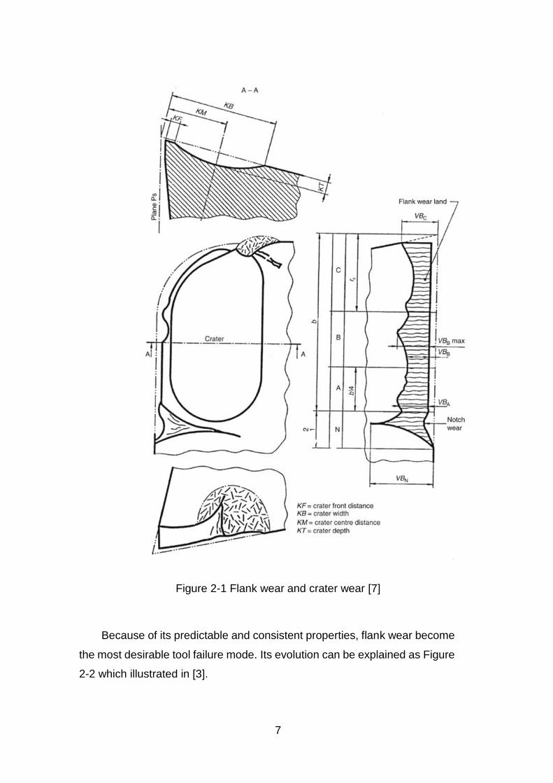
Figure 2-1 Flank wear and crater wear [7]
Because of its predictable and consistent properties flank wear become
the most desirable tool failure mode Its evolution can be explained as Figure
2-2 which illustrated in [3]
8
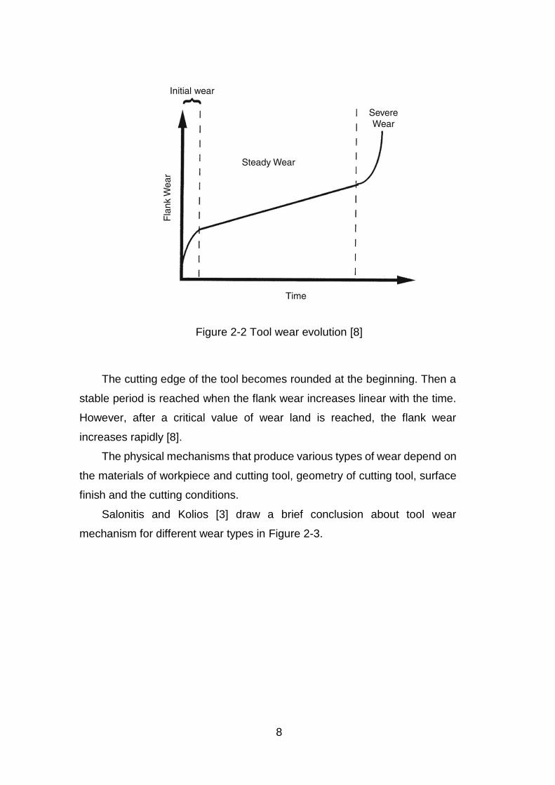
Figure 2-2 Tool wear evolution [8]
The cutting edge of the tool becomes rounded at the beginning Then a
stable period is reached when the flank wear increases linear with the time
However after a critical value of wear land is reached the flank wear
increases rapidly [8]
The physical mechanisms that produce various types of wear depend on
the materials of workpiece and cutting tool geometry of cutting tool surface
finish and the cutting conditions
Salonitis and Kolios [3] draw a brief conclusion about tool wear
mechanism for different wear types in Figure 2-3
9
Figure 2-3 Tool wear mechanism for different wear types [3]
Wang et al [8] explained each wear mechanism carefully and provided
methods to prevent certain type of wear It is mentioned that using one
equation to describe both adhesive and abrasive wear is possible [9]
V =119870119908119873119871119904
119867 (2-1)
Where V is the volume of material worn away 119870119908 is the wear coefficient
119873 is the force normal to the sliding interface 119871119904 is the slid distance and 119867 is
the penetration hardness of the tool
This equation shows some effective methods of controlling wear due to
adhesive and abrasive wear mechanisms
Increasing the hardness 119867 of the cutting tool is the simplest way
Choosing a material with higher hardness and coating the surface of the
cutting tool are both effective way to prevent wear Other than that reducing
cutting force which is 119873 can also decrease wear rate under these conditions
Decreasing cutting speed is another way to diminish the wear rate The
cutting speed has two major effects on the tool wear rate First of all the
sliding distance 119871119904 has a positive relationship with the cutting speed
Secondly the temperature raises on the cutting tool as the increasing the
cutting speed which reduces the hardness of the tool [8]
10
Plastic deformation of the cutting tool edge is also caused by this thermal
softening phenomenon [8]
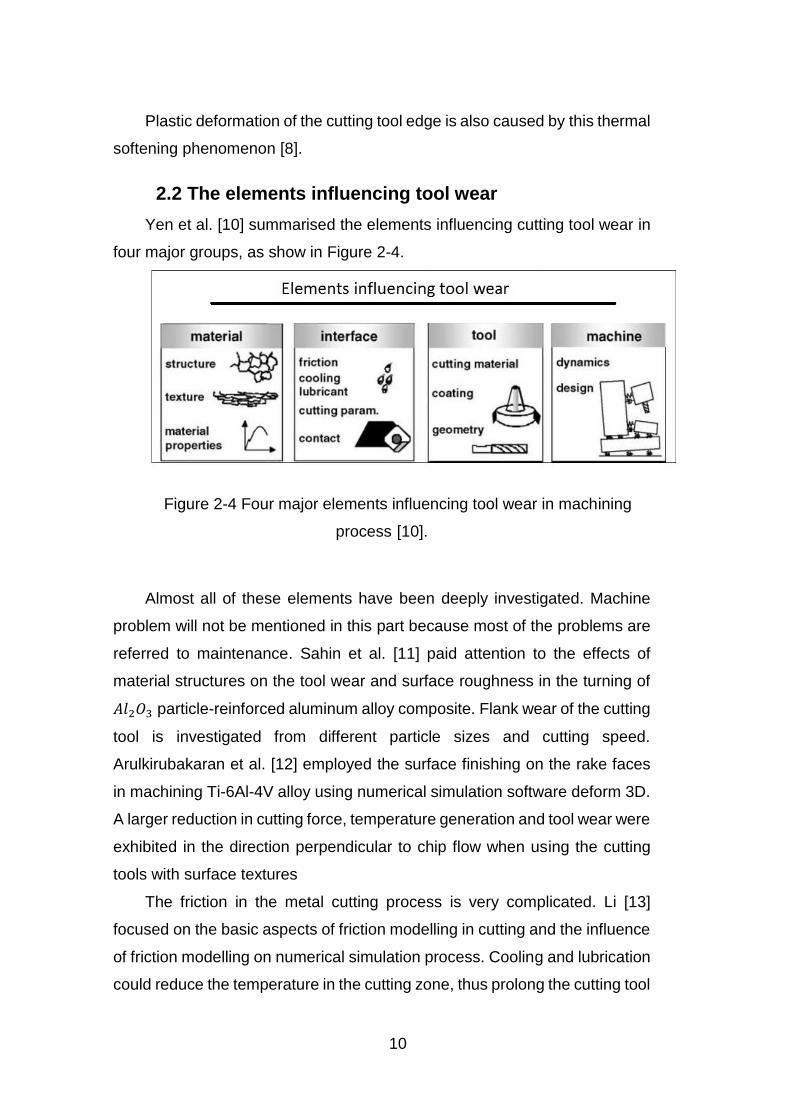
22 The elements influencing tool wear
Yen et al [10] summarised the elements influencing cutting tool wear in
four major groups as show in Figure 2-4
Figure 2-4 Four major elements influencing tool wear in machining
process [10]
Almost all of these elements have been deeply investigated Machine
problem will not be mentioned in this part because most of the problems are
referred to maintenance Sahin et al [11] paid attention to the effects of
material structures on the tool wear and surface roughness in the turning of
11986011989721198743 particle-reinforced aluminum alloy composite Flank wear of the cutting
tool is investigated from different particle sizes and cutting speed
Arulkirubakaran et al [12] employed the surface finishing on the rake faces
in machining Ti-6Al-4V alloy using numerical simulation software deform 3D
A larger reduction in cutting force temperature generation and tool wear were
exhibited in the direction perpendicular to chip flow when using the cutting
tools with surface textures
The friction in the metal cutting process is very complicated Li [13]
focused on the basic aspects of friction modelling in cutting and the influence
of friction modelling on numerical simulation process Cooling and lubrication
could reduce the temperature in the cutting zone thus prolong the cutting tool
11
life However the cycle of heat and cooling on the cutting tool will cause
thermal fatigue and eventually lead to failure
Cutting tool life empirical models can provide some clues to the
importance of cutting parameters Taylorrsquos equation is the first cutting tool life
model It can be expressed as the simple relationship between cutting speed
(119881) and tool life (119879) [14]
119881119879119899 = 119862 (2-2)
Where n and 119862 are constants The exact number depends on feed
depth of cut workpiece material and cutting tool material From Taylorrsquos
equation cutting speed plays an important role in the machining process
Due to its limitation Taylorrsquos equation was changed into different kinds of
forms where other cutting parameters are considered One of these examples
is [15]
119881119879119899119891119898119889119901 = 119862 (2-3)
Where 119881 is the cutting speed 119879 is the tool life 119891 is the feed rate and 119889
is the depth of cut Constants 119899m p and C depend on the characteristics of
the process and are experimentally derived Davis [16] compared the
properties of different cutting tool materials in Figure 2-5 and suggested about
the tool selection methodology shown as Figure 2-6 which is very useful for
the manufacturing engineers
12
Figure 2-5 Properties of cutting tool materials [16]
Figure 2-6 Methodology for cutting tool selection [16]
13
Lo [17] investigated the effect of rake angle on the cutting forces and
chip formation The findings indicated the negative correlation between rake
angle and cutting force and equivalent stress The increasing of rake angel
will also decrease the strength of the cutting tool A balanced point should be
found according to the workpiece material The geometry of the cutting tool
has a closed relationship with the chip formation temperature distribution and
stress distribution In return they will affect the tool wear evolution
23 Tool life and wear evolution models
Arranging cutting experiments under different conditions (such as feed
rate cutting speed) is the normal method to acquire the data for building the
tool wear model Design of experiments (DOE) and response surface
methodology (RSM) are two optimization techniques for analyzing the tool
wear data [10]
Attanasio et al [18] applied the RSM technique to establish the models
for predicting flank wear (VB) and crater depth (KT) The AISI 1045 steel bars
is the workpiece material and uncoated tungsten carbide (WC) is the cutting
tool material under turning process The models were expressed as
119881119861(119881119888 119891 119905) = (minus070199 + 000836119881119888 + 188679119891 + 000723119905 minus
0000021198811198882 minus 3899751198912 minus 0002881199052 minus 0001697119881119888119891 + 000015119881119888119905 +
002176119891119905)2 (2-4)
119870119879(119881119888 119891 119905) = 119890119909119901(minus32648 minus 00367119881119888 + 56378119891 + 04999119905 +
000011198811198882 + 1106951198912 minus 004831199052 + 001257119881119888119891 + 00005119881119888119905 +
01929119891119905)2 (2-5)
Where 119881119888 is the cutting speed 119891 is the feed rate 119905 is the cutting time
Camargo et al [19] also adopted the RSM technology to investigate the
difference between the full wear model and the reduced wear model when
considering the effect of cutting speed and feed rate
However a lot of experiments will be required to achieve a relative
accurate empirical model Although it costs a lot of money and time the final
results may only can be used in a narrow area such as the specific workpiece
material and cutting tool material
14
Cutting tool life model is another kind of empirical model used to predict
the cutting tool performance in the cutting process Taylorrsquos equation is the
most famous one and has already been introduced in the section 22 Despite
the simplicity of the cutting tool life model the constants in the life model can
only be acquired from experiments The limitation on cutting conditions is
another drawback of these kind of models Furthermore as for the managers
of a manufacturing company cutting tool wear evolution is more interesting
to them Due to this some wear rate models were built in the recent few
decades
Ceretti et al [20] found out the constants through experiments based on
the abrasive wear model suggested by [21] which is given by
119885119860119861 = 11987011199011198861119907119888
1198871 ∆119905
1198671198891198881 (2-6)
Where 119885119860119861 is the abrasive wear depth 1198701is the coefficient determined by
experiments 119901 is the local pressure 119907119888 is the local sliding velocity ∆119905 is the
incremental time interval 119867119889 is the cutting tool hardness 1198861 1198871 1198881 are the
experimental constants
Takeyama and Murata gave out an abrasive wear and diffusive wear rate
model in [22]
119889119882
119889119905= 119866(119881 119891) + 119863119890119909119901(minus
119864
119877119879) (2-7)
Where G D is constants 119889119882
119889119905 is the wear rate volume loss per unit contact
area per unit time 119881 is the cutting speed 119864 is the process activation energy
R is the universal gas constant T is the cutting temperature
Usui et al considered adhesive wear in [23]
119889119882
119889119905= 119860120590119899119907119904exp (minus119861
119879frasl ) (2-8)
Where119860 119861 are the constants 120590119899 is the normal stress 119907119904 is the sliding
velocity 119879 is the cutting temperature
Luo et Al [24] combined the abrasive wear rate from [25] and diffusive
wear from [26]
119889119908
119889119905=
119860
119867
119865119891
119881119891 119881119904 + 119861119890119909119901(
minus119864
119877119879119891) (2-9)
15
Where 119889119908
119889119905 is the flank wear rate 119860 is the abrasive wear constant 119867 is the
hardness of the cutting tool material 119865119891 is the feed force 119881 is the cutting
speed 119891 is the feed rate 119881119904 is the sliding speed B is the diffusive wear
constant 119864 119877 119879119891 are process activation energy universal gas constant and
cutting temperature in the tool flank zone respectively
This model is the enhancement of the model of Takeyama and Murata
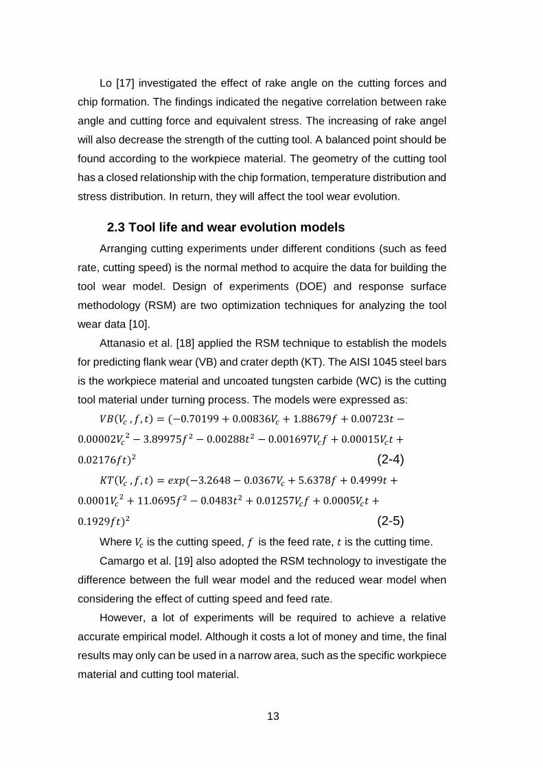
Paacutelmai [27] concluded the tool wear rate models which is shown in Table
2-1
Table 2-1 Tool wear rate models
Shaw and Dirke (1956) V = k119865119899
3120590119910119871
Trigger and Chao (1956) k = 1198961119890119909119901 minus119864
119877119879
Takeyama Murata (1963) 119889119882
119889119905= 119866(119881 119891) + 119863119890119909119901(minus
119864
119877119879)
Usui et al (1984) 119889119882
119889119905= 119860120590119899119907119904exp (minus119861
119879frasl )
Zhao et al (2002) VB = 1198963 (2119907119888
1198872 tan 120572119888)
1
3(
119865119905119905119888
119867(119879))
1
3
119867(119879) = 11988811198793 + 11988821198792 + 1198883119879 + 1198884 (1198881 1198882 1198883 1198884 119886119903119890 119888119900119899119904119905119886119899119905119904)
Luo et al (2005) 119889119908
119889119905=
119860
119867
119865119891
119881119891 119881119904 + 119861119890119909119901(
minus119864
119877119879119891)
Astakhov (2006) ℎ119904 =119889ℎ119903
119889119878=
(ℎ119903minusℎ119903minus119894)100
(119897minus119897119894)119891
Attanasio et al (2008) 119889119882
119889119905= 119863(119879)119890119909119901 (minus
119864
119877119879)
119863(119879) = 11988911198793 + 11988921198792 + 1198893119879 + 1198894 1198891 1198892 1198893 1198894 119886119903119890 119888119900119899119904119905119886119899119905119904
The empirical model is a powerful tool when a new finite element model
using this model is validated by the experiments These models can be used
directly by the manufacturing companies
16
24 Analytical models
Analytical models are mathematical models which have a closed form
solution These models are usually adopted by the numerical models to
describe the condition of a system
However this is by no way means to say that numerical models are
superior to the analytical models In some simple system the solution in the
analytical model is fairly transparent but for more complex systems the
analytical solution can be very complicated For those used to the
mathematics the analytical model can provide a concise preview of a models
behavior which is hidden in the numerical solution On the other hand
numerical model could show out the graphs of important process parameters
changing along with the time which are essential for people to understand
Since analytical model is the foundation of a numerical model
continuing working on the analytical model is vital Even though it can be
sure that no analytical model in cutting process is universally accepted or
employed However the analytical models in many papers reveal the
mechanics of machining and should be considered as the prospective models
before moving on to numerical or any other kinds of machining modeling Two
typical analytical models will be discussed in following shear plane models
and slip-line models
241 Shear plane models
Ernst and Merchant had done a great work on the shear plane models
[28] The idea is the chip will be formed along a single plane inclined at the
shear angle The formation of a continuous chip can be illustrated by a simple
model of a stack of cards In the equilibrium analysis the chip is regarded as
the rigid body and the shear stress is the same as the material flow stress
along the shear plane [5]
The Merchantrsquos circle force diagram is used to calculate the forces on
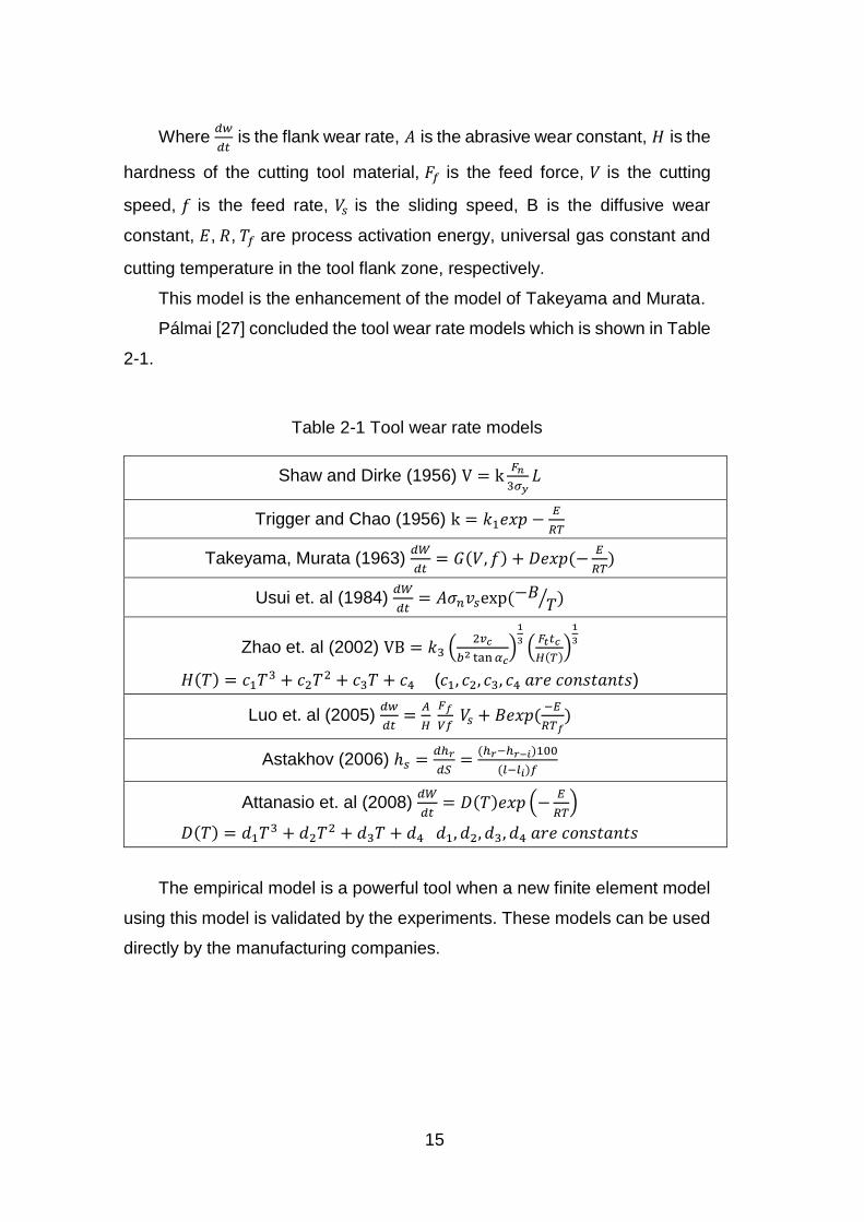
the chip-tool interface and across the shear plane As Show in Figure 2-7
17
Figure 2-7 Merchantrsquos circle [28]
All forces are concentrating on the tool tip The resultant force F can be
resolved in two components the force normal to the tool face (119865119873) and force
along the tool face (119865119865) On the other hand it can be decomposed into 119865119878119873
and 119865119878 which are normal and along the shear plane respectively Furthermore
it can be represented by the cutting force 119865119888 and the thrust force 119865119905 Finally
the shear angle φ rake angle γ the mean friction angle between chip and
tool ρ are shown
Suppose μ is the mean friction coefficient then ρ and μ can be related in
the equation
ρ = arctan(μ) = arctan (119865119865
119865119873frasl ) (2-10)
According to the upper bound condition a shear angle needs to be found
to reduce cutting work to a minimum The work done is proportion to the
cutting force thus the relationship between the cutting force with the shear
angle needs to be found and then using the differential method to obtain the
equation when Fc is a minimum
18
From the Merchant circle the relationship between cutting force 119865119888 and
resultant force 119865 is apparent
119865119888 = 119865 cos(120588 minus 120574) (2-11)
On the other hand shear force along the shear plane can be expressed
in two ways
119865119904 = 119865 cos(120593 + 120588 minus 120574) (2-12)
119865119904 = 120591119904119860119904 =120591119904119860119888
sin 120593 (2-13)
Where 120591119904 is the shear strength of the workpiece material on the shear
plane 119860119904 is the cross-sectional area of the shear plane and 119860119888 is the cross-
sectional area of the un-deformed chip
From the equation (2-12) and (2-13) the resultant force can be written
119865 =120591119904119860119888
sin 120593∙
1
cos(120593+120588minus120574) (2-14)
So the cutting force can be concluded as
119865119888 =120591119904119860119888
sin 120593∙
cos(120588minus120574)
cos(120593+120588minus120574) (2-15)
The cutting force is the function of shear angle using the differential
method and in order to minimize the cutting force the differential equation
equal to zero Then
2φ + ρ minus γ = 1205872frasl (2-16)
It is a brief equation to predict the shear angle but cannot be validated
by experiments Merchant considered the normal stress of the shear plane 120590119904
will affects the shear stress 120591119904 In the modified model a new relation is shown
as
120591119904 = 1205910 + 119896120590119904 (2-17)
Where k is the constant and regarded as the slope between τ and σ
According to this new theory the final equation is
2φ + ρ minus γ = 119862 (2-18)
Where 119862 is the constant depend on the workpiece material
19
242 Slip-line models
A slip-line is a line usually curved and along which the shear stress is the
maximum A complete set of slip-lines in the plastic region form a slip-line
field
For classic slip-line field models in order to simplify the governing
equations several assumptions are made
Plane-strain deformation the model can be only used in the
orthogonal metal cutting
Rigid-plastic work material The material shows no elastic
deformation and shear flow stress does not change with strain
strain-rate and temperature
Quasi-static loading A static load is time independent Note that a
quasi-static condition for one structure may not quasi-static for
another
No temperature changes and no body force
There are two rules that the slip-line field theory must follow in order to
construct a slip-line field for a particular case [5]
First of all the boundary between a part of a material that is plastically
loaded and another that has not yielded is a slip-line
Another rule is that slip-lines must intersect with free surfaces at 45deg
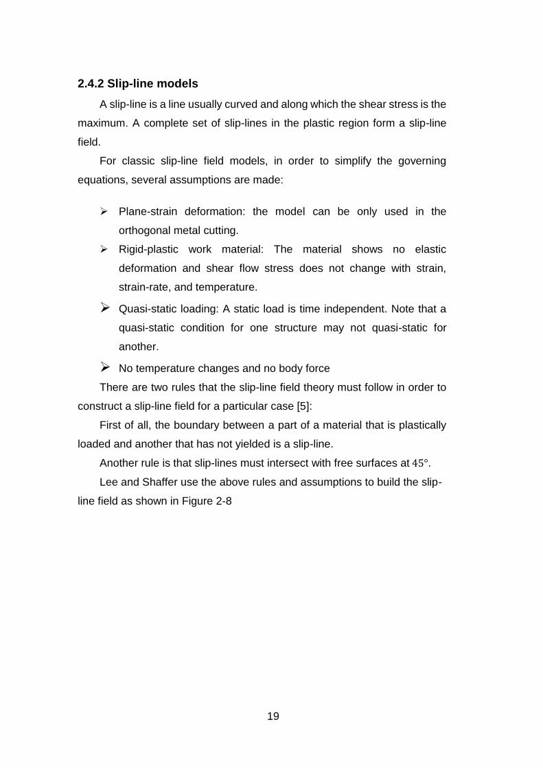
Lee and Shaffer use the above rules and assumptions to build the slip-
line field as shown in Figure 2-8
20
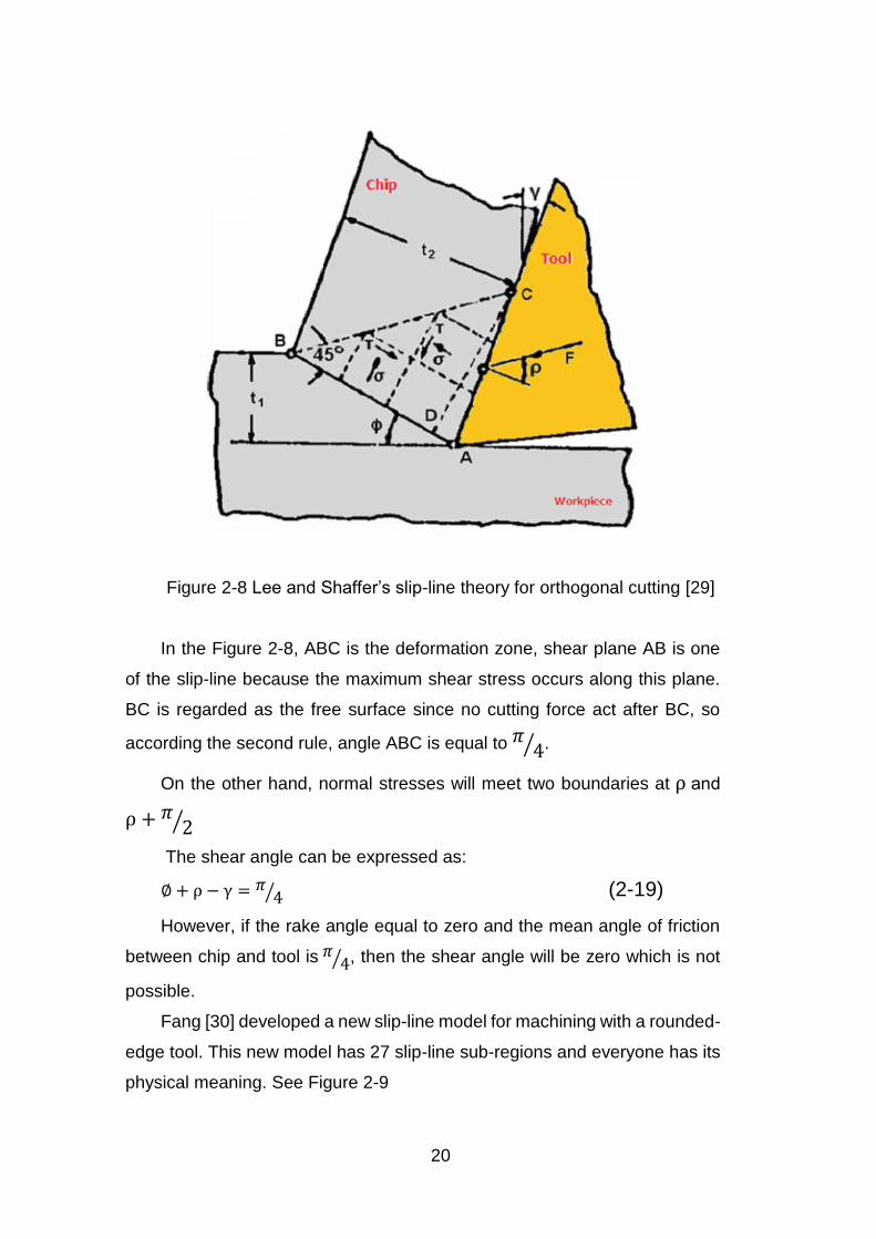
Figure 2-8 Lee and Shafferrsquos slip-line theory for orthogonal cutting [29]
In the Figure 2-8 ABC is the deformation zone shear plane AB is one
of the slip-line because the maximum shear stress occurs along this plane
BC is regarded as the free surface since no cutting force act after BC so
according the second rule angle ABC is equal to 1205874frasl
On the other hand normal stresses will meet two boundaries at ρ and
ρ + 1205872frasl
The shear angle can be expressed as
empty + ρ minus γ = 1205874frasl (2-19)
However if the rake angle equal to zero and the mean angle of friction
between chip and tool is 120587 4frasl then the shear angle will be zero which is not
possible
Fang [30] developed a new slip-line model for machining with a rounded-
edge tool This new model has 27 slip-line sub-regions and everyone has its
physical meaning See Figure 2-9
21
Figure 2-9 Fangrsquos model [30]
Furthermore the model can explain nine effects that occur in the
machining including the size effect and shear zone Eight groups of
machining parameters can be predicted simultaneously including cutting
force chip thickness and shear stain Eight slip-line models developed during
the last six decades such as Merchantrsquos and Lee and Shafferrsquos can be
merged into the new model See Figure 2-10
22
Figure 2-10 Eight special cases of new slip-line model [30]
Arrazola etal [31] made a conclusion about analytical models and gave
out the equations for calculating the main cutting parameters which is a good
guidance for new learners to understand the modelling process
23
25 Finite element method
Finite element method is widely used for investigating the cutting process
due to its flexibility and efficiency Four purposes can be distinguished in the
published papers impacts on workpiece material including the residual stress
chip formation process strain stress and temperature distribution in the
workpiece effects on the cutting tool such as tool wear temperature
distribution on the cutting tool and cutting tool design building the finite
element model such as different workpiece material models friction models
others
Abboud et al [32] studied the effect of feed rate and cutting speed on
residual stresses in titanium alloy Ti-6Al-4V using the orthogonal model
Arulkirubakaran et al [33] made an attempt to reduce detrimental effects on
titanium alloy Ti-6Al-4V using surface textures on rake face of the tool Ceretti
et al [20] investigated the influence of some cutting parameter such as
cutting speed rake angel in a plane strain cutting process using FE code
DEFORM 2D Chiappini et al [34] studied of the mechanics of chip formation
in spindle speed variation(SSV) machining Hadzley et al [35] studied the
effect of coolant pressure on chip formation cutting force and cutting
temperature A reduced cutting force and temperature was witnessed due to
the increasing of the coolant pressure Kalyan and Samuel [36] developed a
FE model to study the effect of cutting edge chamfer on high speed turning
of AlMgSi (Al 6061 T6) alloy and validated by experiments Lei et al [37]
simulated continuous chip formation for 1020 steel under a plane strain
condition with a new material constitutive model using finite element method
Li et al [38] investigated the effects of crater wear on the cutting process
using Abaqus by change the geometry of the cutting tool A significant impact
of crater wear size on the chip formation and contact stresses is observed
List et al [39] examined the strain and strain rate variations in the primary
shear zone and investigated the distribution of velocity Liu and Melkote [40]
investigated the relationship between cutting tool edge radius and size effect
by developing finite element model on Al5083-H116 alloy under orthogonal
cutting condition Lo [17] investigated the effect of tool rake angle on cutting
24
force chip geometry stress distribution residual stress and surface quality
of the workpiece material Mamalis et al [41] presented a coupled thermo-
mechanical orthogonal cutting model using commercial finite element
package MARC to simulate continuous chip formation under plane-strain
condition Maranhatildeo and Paulo Davim [42] built a thermal and mechanical
model for AISI 316 determined the effect of the friction coefficient on
important process parameters such as temperature and stress along the tool-
chip interface Shet and Deng [43] developed an orthogonal metal cutting
model to investigate the residual stress and strain distribution using FEM in
the workpiece under plane strain conditions Thepsonthi and Oumlzel [44]
studied the effect of cutting tool wear on process variables when milling on
Ti-6Al-4V
Filice et al [45] proposed an effective FE model including both flank and
crater wear using polynomial method Hosseinkhani [46] built a finite element
model using Abaqus to investigate the change of contact stress plastic
deformation and temperature distribution based on different worn cutting tool
geometry It is shown that the flank wear size has the larger impact on the
tertiary deformation region than the other two The highest temperature point
on the cutting tool transferred from rake face to flank face due to the flank
wear Kumar et al [47] constructed an optimal design method of end mill
cutters for milling Titanium alloy Ti-6Al-4V using FE analysis Salvatore et al
[48] presented a new method for predicting tool wear evolution during cutting
process Yen et al [10] developed a methodology to simulate the cutting tool
life and wear evolution under orthogonal cutting condition using FEM
Lin and Lin [49] established a large deformation thermo-mechanical FE
model for oblique cutting process Liu et al [50] developed a new constitutive
model considering the influencing of micro damage in the workpiece material
based on ZerillindashArmstrong (Z-A) model Owen and Vaz [51] presented a FE
model about the effect of adiabatic strain concentration on the failure of
material using adaptive method Oumlzel [52] developed an orthogonal cutting
model to simulate the continuous chip formation based on updated
Lagrangian FE formulation and investigated the stress distributions on the
25
cutting tool under different friction models Patil et al [53] studied the
influence of ultrasonic assisted turning (UAT) using 2D FE transient
simulation in DEFORM framework this method seemed improving all except
the surface roughness comparing with continue turning process Umbrello
[54] investigated the machining of Ti-6Al-4V for both conventional and high
speed cutting regimes using finite element analysis (FEA) Wang et al [55]
proposed a new approach to predict optimal machining conditions for most
energy-efficient machining of Ti-6Al-4V
Bil et al [56] compared various finite element packages such as MSC
Marc Deform 2D and Thirdwave AdvantEdge using an orthogonal cutting
model and found out that no model can acquire acceptable results for all
process parameters
26 Key findings and research gap
It can be concluded from the papers that
Most of the published papers are focused on the effects on
workpiece material
Cutting tool wear evolution and temperature distribution are
commonly investigated in papers
Cutting tool is usually regarded as a rigid body in the simulation
process
Although almost all the aspects of cutting process are studied using FEM
the effects of various cutting parameters such as cutting speed tool edge
radius cutting depth and tool wear on the cutting tool are neglected by most
researchers On the other hand the wear evolution models and tool life
models cannot be used in the workshop efficiently and conveniently
Machining power maybe the choice In this thesis these two aspects will be
investigated
26
3 Finite element simulation of metal cutting
31 Introduction
Experiments analytical models and finite element methods are
commonly adopted in metal cutting research area At the beginning
experiments were the most widely used method to study the impacts of
various cutting process parameters However it is very expensive and time
consuming Analytical models were adopted to predict the cutting tool life and
the mechanisms behind the cutting process such as chip formation and size
effect It helps a lot but cannot be used for complicated cutting conditions
Finite element method becomes predominant in the cutting process research
area due to the development of computer technology and commercial finite
element software Various parameters and characteristics of the cutting
process such as temperature and stress distribution strain cutting force can
be predicted which may be hard to obtain through experiments or analytical
methods
In order to build a simulation model using FEM the following aspects
need to be considered
Select a suitable finite element package according to the explicit
and implicit method and motion description method
Choice of workpiece material
Workpiece material constitutive model and damage model
Chip formation and separation criteria
Friction model
The reasons can be listed as
Only a few finite element codes can be used for dynamic process
such as cutting process
Workpiece material should be chosen according to the
requirement in the company
The workpiece material model should represent the flow stress
under high strain strain rate and temperature The damage model
27
is part of the material property which need to be considered
carefully
Chip formation has a close relationship with the surface quality
tool life and machining stability
Friction is quite complicated in the contact face between cutting
tool and the chip Reflecting the true friction condition is vital to
the simulation accuracy
32 The selection of finite element package
There are many finite element codes existing in the market which can be
used in engineering area In order to find the right one for the cutting process
two important concepts must be clarified in the first place explicit and implicit
method and motion description method
321 Explicit and implicit
3211 Explicit and implicit solution method
Explicit use central different formula to solve the (t + Δt) using information
at the time t [57] while in implicit solution the condition of (t + Δt) determine
the state of (t + Δt) [58] Backward Euler method is an example of implicit
time integration scheme while forward Euler method or central difference are
examples of explicit time integration schemes
Backward Euler method is according to backward difference
approximation [59] and can be expressed as
119910119905+∆119905 = 119910119905 + ℎ119891(119910119905+∆119905 119909119905+∆119905) (5-1)
Which confirms the statement that the condition of (t + Δt) determine the
state of (t + Δt)
Forward Euler method uses forward difference approximation as shown
below
119910119905+∆119905 = 119910119905 + ℎ119891(119910119905 119909119905) (5-2)
It is clearly shown that the information at the time (t + Δt) depends on
the condition of the time t
Another explicit time integration scheme is central difference method
See Figure 5-1
28
Figure 5-1 Explicit time scheme (every time distance is ∆1199052)
Central different formula can be displayed as
119899 =1
2∆119905(119906119899+1 minus 119906119899minus1) (5-3)
119899 =1
∆119905(
119899+1
2
minus 119899minus
1
2
) =1
∆119905(
119906119899+1minus119906119899
∆119905minus
119906119899minus119906119899minus1
∆119905) =
1
∆1199052(119906119899+1 + 119906119899minus1 minus 2119906119899)
(5-4)
When consider linear dynamic situation equilibrium at time 119905119899
119872119899 + 119862119899 + 119870119906119899 = 119877 (5-5)
Put (5-3) (5-4) into (5-5)
(119872 +∆119905
2119862) 119906119899+1 = ∆1199052119877 minus (∆1199052119870 minus 2119872)119906119899 minus (119872 minus
∆119905
2119862)119906119899minus1
(5-6)
Where 119906 is the displacement vector is the velocity vector is the
acceleration vector R is vector of the applied load M is the mass matrix C
is the damping matrix and K is the stiffness matrix
It also shows that the situation of (t + Δt) rely on the condition of the time
t
29
3212 Iterative scheme
The implicit procedure uses the Newton-Raphson method to do the
automatic iteration [60] The main idea can be seen from Figure 5-2
Figure 5-2 Newton-Raphson iterative method
119891prime(1199090) =119891(1199090)
1199090minus1199091 (5-7)
1199091 = 1199090 minus119891(1199090)
119891prime(1199090) (5-8)
This process will repeat as
119909119899+1 = 119909119899 minus119891(119909119899)
119891prime(119909119899) (5-9)
Until 119909119899+1 119909119899 are close enough to each other
On the other hand explicit procedure demands no iteration and during
each time increment the change of time rates is considered constant Unlike
implicit solver the stability of explicit integration relies on the highest
eigenvalue of the system ( 120596119898119886119909) [61] and time step should meet the
equation below
∆119905 le2
120596119898119886119909(radic1 + 1205762 minus 120576) (5-10)
Where 120576 is the critical damping fraction this ensure that the time step ∆119905
is smaller than the time of elastic wave passes one mesh
In non-linear situation implicit solver may need many iterations for an
increment smaller time steps will be used and convergence may be
impossible [58] As shown above the convergence of explicit only depends
30
on ∆119905
3213 Choice in cutting process
In the cutting process large deformation occurs in the workpiece
material Large deformation is regarded as geometrical nonlinearity [62] Both
implicit and explicit methods can be used in nonlinear situations [60] Rebelo
et al [63] argue that 2D problems are suitable for implicit method and
complicated contact problems should use explicit methods for efficiency
Implicit method can suffer converging problem during large deformation
processes and surface contact problems ([58] in [61636465]) Due to the
converging issue explicit is the better choice tackling the contact and large
deformation problem Harewood [58] argues that minimizing the time step will
increase the computer running time and may result in divergence The
drawback of explicit method is stability and short time duration decreasing
the time step and limit the kinematic energy are possible solutions [58] Yang
et al [61] also argue that for high-speed dynamic events explicit solver is
more suited
Based on these findings this thesis will use the explicit method to solve
the finite element model in manufacturing process
322 Description of motion
Traditionally speaking in structure mechanics Lagrangian description is
adopted to solve the deformation problems [66] The movement of each
individual node is solved as a function of the material coordinates and time
Comparing with the pure Eulerian approach the only need to satisfy fewer
governing equations [66] This is mainly due to the simple way to track the
forming process when using the pure Lagrangian approach [66]
However a large deformation of the material may happen in the cutting
area without frequent remeshing operations Remeshing process is
conducted to acquire accepted accuracy for the simulation even though it will
need a long computing time [66] However in pure Lagrangian approach it
is difficult to describe the boundaries of sharp edges or corners since the
edge may move during the simulation process [66]
Eulerian description is widely used in fluid dynamics [67] The movement
31
of the elements is regarded as the relationship between spatial coordinate
and time [68] In the Eulerian description reference mesh is adopted to trace
the movement of material without any distortion [68] However if two or more
materials exist in the Eulerian domain numerical diffusion may occur [68]
Because of the advantages and disadvantages of each method a new
technology occurs to combine these two which is known as Arbitrary
LagrangianndashEulerian (ALE) description Donea et al [67] present a one-
dimensional picture about the difference of these three descriptions Show as
Figure 5-3
Figure 5-3 One dimensional example of lagrangian Eulerian and ALE
mesh and particle motion [67]
Khoei et al [69] divided the uncoupled ALE solution into 3 different
phases Material (Lagrangian) phase Smoothing phase and Convection
(Eulerian) phase The Lagrangian phase is used to acquire the convergence
32
at each time step The Eulerian phase was adopted to get a regular mesh
configuration In the first place the nodal positions were relocated arbitrarily
regardless of the FE mesh In the smoothing phase nodesrsquo coordinate value
was updated according to the setting of level which may different from the
previous one
Donea et al [67] argued that in ALE any mesh-smoothing algorithm can
be used once the topology is fixed to improve the shape of the elements
Lagrangian description is used in this simple model
323 Selection of Finite element package
More and more commercial FE codes are developed to simulate the
physical world in engineering field
For metal cutting simulation packages like Abaqus AdvantEdge
Deform 2D3D and Ls-dyna using explicit and Lagrangian description are
widely used both in research area and industrial field Software mainly using
the implicit method such as ANSYS cannot be used to simulate the metal
cutting process
Pop and Bianca [70] have made a conclusion about the most widely used
finite element package from 1995 to 2013 The result is shown Figure 4-4
Figure 5-4 The usage ratio of different finite element packages [70]
33
Instead of talking about the differences between those packages which
have already mentioned in the work of Kilicaslan [71] an example will be
given for each popular package
Deform 2D3D which is regarded as the most popular FE software for
metal cutting in the industry field was first released in 1989 as the 2D
workstation version In 1993 DEFORM-3D was released based on
engineering workstations to solve full three dimensional problems
Kohir and Dundur [72] used the DEFORM 2D to investigate the influence
of flank wear on the cutting force stress and temperature distribution
Temperature distribution in the workpiece and cutting tool is shown in
Figure 5-5
Figure 5-5 Temperature distribution when flank wear inclination=12deg
wear land=2mm [72]
AdvantEdge uses a virtual testing environment to understand the inner
causes of the tool performance and improve the cutting tool design
Temperature and stress analysis due to tool wear is a strong point of this
code
Maranhatildeo and Paulo Davim [42] use the AdvantEdge to investigate the
34
effect of the friction coefficient on the tool-chip interface in the cutting process
The result of maximum shear stress in cutting tool workpiece material
and chip can be seen below in Figure 5-6
Figure 5-6 Maximum shear stress in the tool and workpiece [42]
Abaqus is firstly released in 1978 and suited for finite element analysis
(FEA) It is widely used in campus and research institutions mainly because
its capacity in material modelling and customization
Hosseinkhani and Ng [46] build an ALE model based on
ABAQUSExplicit The model was validated by experiment results the
influence of tool wear on process variables were investigated
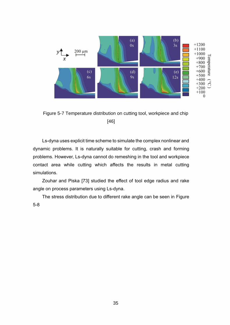
Temperature distribution on cutting tool workpiece and chip can be seen
in Figure 5-7
35
Figure 5-7 Temperature distribution on cutting tool workpiece and chip
[46]
Ls-dyna uses explicit time scheme to simulate the complex nonlinear and
dynamic problems It is naturally suitable for cutting crash and forming
problems However Ls-dyna cannot do remeshing in the tool and workpiece
contact area while cutting which affects the results in metal cutting
simulations
Zouhar and Piska [73] studied the effect of tool edge radius and rake
angle on process parameters using Ls-dyna
The stress distribution due to different rake angle can be seen in Figure
5-8
36
Figure 5-8 Von Mises stress field for tool with different rake angle a) -
5 degb) 0 deg c) 5 degd) 10 deg [73]
As one of these commercial FE packages Ls-dyna is chosen for this
thesis because of its ability in solving dynamic problems and accessibility to
the author on campus This software is used to investigate the effect of cutting
tool wear on cutting force temperature and stress distribution
33 Workpiece material and different models for
modelling
331 The chosen of workpiece material
In this thesis Ti-6Al-4V is chosen as the workpiece material mainly due
to the following reasons
37
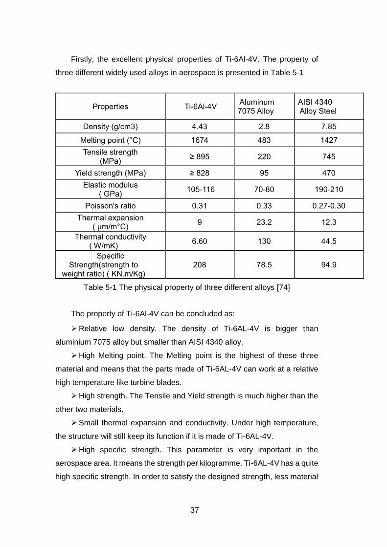
Firstly the excellent physical properties of Ti-6Al-4V The property of
three different widely used alloys in aerospace is presented in Table 5-1
Table 5-1 The physical property of three different alloys [74]
The property of Ti-6Al-4V can be concluded as
Relative low density The density of Ti-6AL-4V is bigger than
aluminium 7075 alloy but smaller than AISI 4340 alloy
High Melting point The Melting point is the highest of these three
material and means that the parts made of Ti-6AL-4V can work at a relative
high temperature like turbine blades
High strength The Tensile and Yield strength is much higher than the
other two materials
Small thermal expansion and conductivity Under high temperature
the structure will still keep its function if it is made of Ti-6AL-4V
High specific strength This parameter is very important in the
aerospace area It means the strength per kilogramme Ti-6AL-4V has a quite
high specific strength In order to satisfy the designed strength less material
Properties Ti-6Al-4V Aluminum 7075 Alloy
AISI 4340 Alloy Steel
Density (gcm3) 443 28 785
Melting point (degC) 1674 483 1427
Tensile strength (MPa)
ge 895 220 745
Yield strength (MPa) ge 828 95 470
Elastic modulus ( GPa)
105-116 70-80 190-210
Poissons ratio 031 033 027-030
Thermal expansion ( micrommdegC)
9 232 123
Thermal conductivity ( WmK)
660 130 445
Specific Strength(strength to
weight ratio) ( KNmKg) 208 785 949
38
can be used for Ti-6AL-4V Thus less fuel will be consumed for an airplane if
Ti-6AL-4V is used rather than other two materials
Secondly it is used more and more in aerospace The components of
the material in Boeing 777 and Boeing 787 are shown in Figure 4-9 and
Figure 4-10 respectively
Figure 5-9 The weight ratio for different materials in Boeing 777 [75]
39
Figure 5-10 The weight ratio for different materials in Boeing 787 [76]
In Boeing 777 which was introduced in 1993 Titanium alloy is only 7
for Boeing 787 which was introduced in 2007 the titanium takes 15 of the
whole material
Thirdly the titanium alloy is very hard to machine When compared with
AISI B1112 steel the rating for Ti-6Al-4V is only 22 which is regarded as
very hard to machine (The rating for AISI B1112 steel is set as 100) Shown
in Table 5-2
Table 5-2 The machining easiness of different alloys [77]
So in this thesis Ti-6AL-4V is taken as the workpiece material
332 The workpiece constitutive model
A workpiece material constitutive model is required to represent the flow
stress under high temperature strain and strain rate condition [50]
40
Several researchers have come up with specific constitutive models to
represent the material property
3321 The JohnsonndashCook (J-C) model
The J-C model is a purely empirical model subjected to large strain by
Johnson amp Cook in 1983 The model for flow stress 120590 can be expressed as
[78]
120590 = 119860 + 1198611205761198991 + 119862119897119899 120576lowast1 minus 119879lowast119898 (5-11)
Where 120576 is the equivalent plastic strain 120576lowast =
0 is the dimensionless
plastic strain rate for 1205760 = 10 119904minus1 and 119879lowast is the homologous temperature And
119879lowast =119879minus1198790
119879119898minus1198790 where 1198790is the reference temperature and 119879119898is a reference melt
temperature 119860 119861 119899 119862 119898 are five material constants 119860 is the initial yield
stress 119861 is the hardening constant 119899 is the hardening exponent 119862 is the
strain rate constant 119898 is the thermal softening exponent
The J-C model is widely used by many works Chen et al [79] used the
J-C model to simulate the chip morphology and cutting force of the titanium
alloy (Tindash6Alndash4V) high-speed machining The model is validated by
experimental results Thepsonthi and Oumlzel [44] used a modified J-C model to
exhibit workpiece flow stress in cutting process as shown in Equation (5-12)
120590 = 119860 + 119861120576119899(1
exp (120576119886)) 1 + 119862119897119899
0 1 minus (
119879minus1198790
119879119898minus1198790)119898D + (1 minus
D)[tanh (1
(120576+119901)119903)]119904 (5-12)
Where D = 1 minus (119879 minus 119879119898)119889 p = (119879119879119898)119887 120590 is flow stress ε is true strain
120576 is true strain rate 1205760 is reference true strain rate (1205760 = 10minus5) The meaning
of other material constants is the same as in the typical J-C model
Sima amp Oumlzel [80] discussed some material constitutive models including
the JndashC material model and in the end a modified J-C model was used to
simulate the material behaviour of Ti-6Al-4V according to the simulation
results
3322 The SteinbergndashCochranndashGuinanndashLund (SCGL) model
The Steinberg-Cochran-Guinan-Lund (SCGL) model is a semi-empirical
model which was established by Steinberg et al [81] under high strain-rate
41
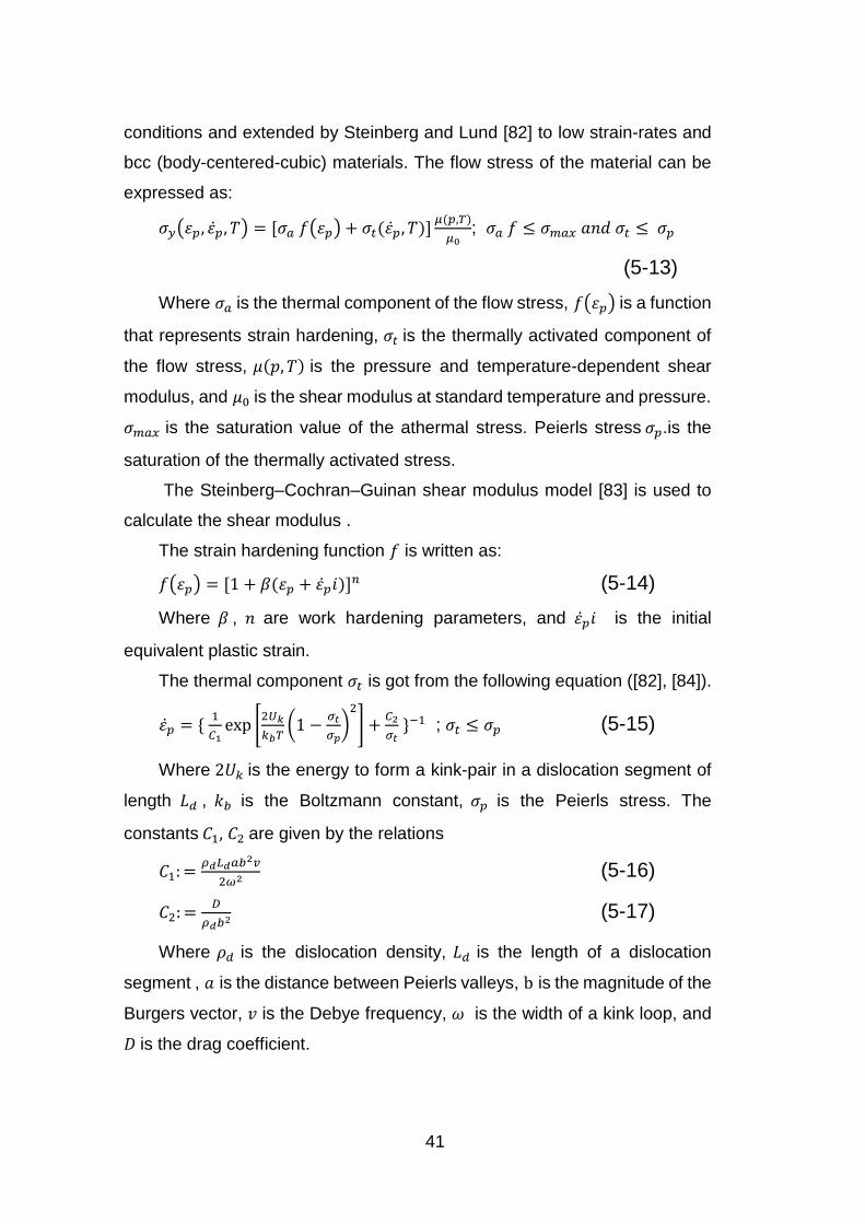
conditions and extended by Steinberg and Lund [82] to low strain-rates and
bcc (body-centered-cubic) materials The flow stress of the material can be
expressed as
120590119910(120576119901 120576 119879) = [120590119886 119891(120576119901) + 120590119905(120576 119879)]120583(119901119879)
1205830 120590119886 119891 le 120590119898119886119909 119886119899119889 120590119905 le 120590119901
(5-13)
Where 120590119886 is the thermal component of the flow stress 119891(120576119901) is a function
that represents strain hardening 120590119905 is the thermally activated component of
the flow stress 120583(119901 119879) is the pressure and temperature-dependent shear
modulus and 1205830 is the shear modulus at standard temperature and pressure
120590119898119886119909 is the saturation value of the athermal stress Peierls stress 120590119901is the
saturation of the thermally activated stress
The SteinbergndashCochranndashGuinan shear modulus model [83] is used to
calculate the shear modulus
The strain hardening function 119891 is written as
119891(120576119901) = [1 + 120573(120576119901 + 120576119894)]119899 (5-14)
Where 120573 119899 are work hardening parameters and 120576119894 is the initial
equivalent plastic strain
The thermal component 120590119905 is got from the following equation ([82] [84])
120576 = 1
1198621exp [
2119880119896
119896119887119879(1 minus
120590119905
120590119901)
2
] +1198622
120590119905 minus1 120590119905 le 120590119901 (5-15)
Where 2119880119896 is the energy to form a kink-pair in a dislocation segment of
length 119871119889 119896119887 is the Boltzmann constant 120590119901 is the Peierls stress The
constants 1198621 1198622 are given by the relations
1198621 =1205881198891198711198891198861198872119907
21205962 (5-16)
1198622 =119863
1205881198891198872 (5-17)
Where 120588119889 is the dislocation density 119871119889 is the length of a dislocation
segment 119886 is the distance between Peierls valleys b is the magnitude of the
Burgers vector 119907 is the Debye frequency 120596 is the width of a kink loop and
119863 is the drag coefficient
42
Based on limited experimental evidence and upon robust first-principle
calculations of the elastic module for diamond Orlikowski et al [85] used the
SCGL model without the effect of strain-rate They performed hydrodynamic
1-D simulations of an isotropic polycrystalline diamond and have compared
them to single crystal diamond experiments as a rough indicator to the
modelrsquos performance A good coherence was found
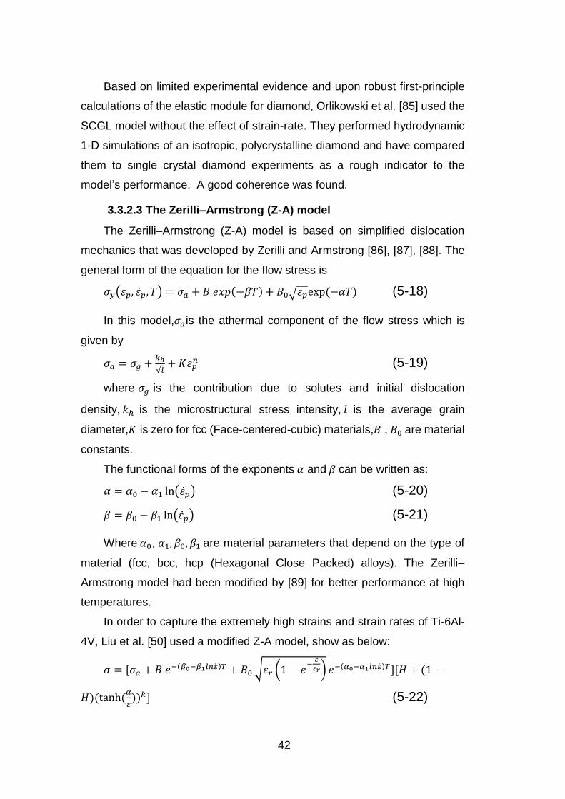
3323 The ZerillindashArmstrong (Z-A) model
The ZerillindashArmstrong (Z-A) model is based on simplified dislocation
mechanics that was developed by Zerilli and Armstrong [86] [87] [88] The
general form of the equation for the flow stress is
120590119910(120576119901 120576 119879) = 120590119886 + 119861 119890119909119901(minus120573119879) + 1198610radic120576119901exp (minus120572119879) (5-18)
In this model120590119886is the athermal component of the flow stress which is
given by
120590119886 = 120590119892 +119896ℎ
radic119897+ 119870120576119901
119899 (5-19)
where 120590119892 is the contribution due to solutes and initial dislocation
density 119896ℎ is the microstructural stress intensity 119897 is the average grain
diameter119870 is zero for fcc (Face-centered-cubic) materials119861 1198610 are material
constants
The functional forms of the exponents 120572 and 120573 can be written as
120572 = 1205720 minus 1205721 ln(120576) (5-20)
120573 = 1205730 minus 1205731 ln(120576) (5-21)
Where 1205720 1205721 1205730 1205731 are material parameters that depend on the type of
material (fcc bcc hcp (Hexagonal Close Packed) alloys) The Zerillindash
Armstrong model had been modified by [89] for better performance at high
temperatures
In order to capture the extremely high strains and strain rates of Ti-6Al-
4V Liu et al [50] used a modified Z-A model show as below
120590 = [120590119886 + 119861 119890minus(1205730minus1205731119897119899)119879 + 1198610 radic120576119903 (1 minus 119890minus
120576
120576119903) 119890minus(1205720minus1205721119897119899)119879][119867 + (1 minus
119867)(tanh (120572
120576))119896] (5-22)
43
Where the failure function is given by the second bracketed term and is
controlled by three strain rate dependent parameters119867 120572 and 119896
This model is validated by experiments under orthogonal cutting
conditions
3324 Evaluation of three models
Banerjee [83] evaluated these three flow stress models on the basis of
one-dimensional tension and compression test varying the temperature and
strain-rate The average maximum absolute errors in yield stresses predicted
by three flow stress models are exhibited in the Table 5-3
Table 5-3 Average maximum absolute errors [83]
Condition
Average Max Error ()
J-C model
SCGL model Z-A model
All Tests 36 64 33
Tension Tests 25 20 19
Compression Tests
45 126 50
High Strain Rate (ge 100 s)
29 22 20
Low Strain Rate (lt 100 s)
45 219 76
High Temperature
(ge 800 K) 43 90 40
Low Temperature (lt
800 K) 20 20 17
average 347 801 364
44
The Johnson-Cook model has the lowest average error in all these
situations Thus Johnson-Cook constitutive model is used as the workpiece
material constitutive model
333 The workpiece damage model
A damage model for cutting process is a part of the Finite Element
simulation It works with the chip separation criteria to simulate the movement
of cutting tool and the material before tool tip Generally the damage model
should contain the damage initiation and damage evolution
For ductile material a uniaxial stressndashstrain curve is used to represent
the principle of material behaviour evolution See Figure 5-11
Figure 5-11 Typical uniaxial stress-strain in case of a ductile metal [90]
3331 Damage initiation
Damage initiation criterion represents the beginning of the material
damage Johnson-Cook shear failure model will be introduced to analyse the
damage initiation in cutting The strain at fracture can be expressed as [91]
120576119891 = max ([1198631 + 11986321198901199091199011198633120590lowast][1 + 1198634119897119899120576lowast][1 + 1198635119879lowast] 119864119865119872119868119873) (5-23)
45
Where 1198631 to 1198635 are failure parameters generally from experiments 120590lowast
is the ratio of pressure divided by effective stress 120590lowast =119901
120590119890119891119891120576lowast =
119864119875119878119874
119901
119864119875119878119874
EPSO
is the Quasi-static threshold strain rate 120576119901 eeffective plastic strain 119879lowast =
119879minus119879119903119900119900119898
119879119898119890119897119905minus119879119903119900119900119898 is the homologous temperature
When a scalar damage parameter ω exceeds 1 the damage is initiated
This parameter is defined as
ω = sum (∆119901
120576119891 )119895nj=1 (5-24)
where ∆120576119901 is the increment of equivalent plastic strain during an
increment of loading j in each integration point
According to equation (5-22) the stress triaxiality 120590lowast damage may be
initiated by strain rate and temperature
3332 Damage evolution
After damage initiation the Hillerborgrsquos fracture energy was used to
control damage evolution With this method the damage evolution process
became more stable and can capture strain localization using large mesh
size [90]
For ductile material if the damage initiation occurs the stressndashstrain
relationship can no longer accurately represents the material behaviour
Hillerborgrsquos fracture energy proposal used a stressndashdisplacement
response after damage initiation to decrease the mesh dependency The
fracture energy is then given as [90]
119866119891 = int 119871120590119889120576119901119865
119901
119861119901 = int 120590119889
119906119865119901
0119901 (5-25)
Where 120576119901 and 120576
119901 are the equivalent plastic strain at points B and F in
Figure 5-11 120590 is the equivalent plastic stress
Through the definition 119866119891 introduced the equivalent plastic displacement
119901 together with the yield stress to control the damage evolution In the finite
element model characteristic length L of the element is required to build the
stressndashdisplacement relationship
Element aspect ratio has an effect on the crack behaviour after damage
46
initiation Elements which have unit aspect ratio are better choice [90]
The scalar stiffness degradation for the linear damage process is given
by
119863 =int 119871119889119901119901
119861119901
119866119891=
int 119889119901
0 119906119901
119866119891 (5-26)
Whereas an exponential damage parameter can evolve according to
D = 1 minus exp (minus int120590
119866119891
119889119906119901
0119901) (5-27)
The formulation of the model ensured that the energy dissipated is equal
to 119866119891 during the damage evolution process In theory only at an infinite
equivalent plastic displacement the damage variable D reaches a value of
one In commercial finite element software D is set as 099 or less to keep
elements active in simulation The plastic equivalent stresses in the material
is given by
σ = (1 minus D) (5-28)
Where is the effective (or undamaged) stress computed in the current
increment It represents stresses that would exist in the material without
damage
Sui and Feng [92] used the Cockroft and Lathamrsquos fracture criterion to
explain the material damage process The criterion can be expressed as
119862119894 = int 120590120576119891
0119889120576 (5-29)
Where 120590 is the maximum flow stress 120576119891 is the fracture strain and 119862119894 is
the material constant
Hambli [93] adopted the Lemaitre damage model to describe the crack
initiation and propagation The damage law is written in an incremental form
=119863119862
120576119877minus120576119863[
2
3(1 + 119907) + 3(1 minus 2119907) (
120590119867
120590119890119902)
2
](120576119890119902)2
119899frasl 119889120576119902 (5-30)
Where 119899 is the hardening exponent and 119907 is the Poissonrsquos ratio 120576119863 is the
threshold logarithmic strain at which damage initiates 120576119877 is the logarithmic
strain value at fracture and 120576119890119902 the logarithmic plastic strain 119863119862 is the critical
damage value at fracture
47
34 Chip formation process
341 Introduction
Despite different kinds of traditional machining process like milling
turning grinding it is the same process of removing material from a blank to
form the chips when a certain chip thickness and depth of cut are reached
By studying the chip formation process researchers and engineers can
obtain the behaviour of workpiece material under pressure specific energy
(the amount of energy required to remove unit volume of work material)
requirement in the machining cutting tool life and the method to get better
surface finish
The form of the chips mainly depends on
The workpiece and cutting tool material
Cutting conditions (Feed speed cutting speed depth of cut and the
use of coolant)
Cutting tool geometry (rake angle cutting edge angle tool cutting
edge inclination chip breaker worn shape)
In this section the basic mechanism of chip formation for four different
types of chip will be discussed in the first place Types of chip morphology
chip separate criteria chip forming process and effect of friction model will be
clarified
342 Chip formation mechanism
In the cutting process the cutting tool will penetrate into the workpiece
material causing elastic and plastic deformation the stress concentration
near the tool tip and the chip deprive from the workpiece When take a close
look at the chip formation process four types of chip morphology could be
identified mainly due to different materialsrsquo flow properties On the other hand
the cutting parameters geometry of the cutting tool even the use of coolant
will also affect the morphology of the chip
Generally there are two ways to distinguish the chip formation process
one is based on the chip morphology known as continuous chips lamellar
chips segment chips and discontinuous chips [57] [94] shown in Figure 5-
48
12 the other is according to the flow property of the workpiece material such
as brittle material and ductile material [95][96]
In the following sections chip morphology will be discussed
Figure 5-12 Four types of chips [94]
3421 Continuous Chips
To form a continuous chip the maximum shear stress for the material
(120590119898119886119909) is bigger than the maximum shear stress in the deformation zone(1205900)
The stress-strain relationship for ductile material is shown in Figure 5-13
49
Figure 5-13 Flow stress property
There will be no fracture happening in the cutting area the
microstructure in the cutting zone tend to be uniform and the metal undergoes
the continuous plastic deformation due to the compression stress Then the
chip will flow up along the rake face of the cutting tool
When using a commercial FEM software to simulate this type of chip (as
shown in Figure 5-14) the shear zone can be clearly seen
Figure 5-14 Continue chip formation
50
Almost the same thickness of the chip is obtained throughout and since
it is very stable during the cutting a best surface finish could be expected
compare to the other types of chip
The continuous chip is most likely to form in the following condition
Ductile material to withstand the plastic deformation
High cutting speed for the smooth flow of the ductile material
Small chip thickness
Positive and large rake angle for the material to flow easily
Sharp cutting edge
Using coolant and lubricating
Small friction between the chip and cutting tool surface
However along the continuous chip a strong and almost uniform shear
stress exists so it is very hard to break this type of chip and may result the
damage of the cutting tool
3422 Lamellar Chips
Lamellar chip is also a result of continuous chip formation process
however some reasons such as the non-uniform microstructure will cause
the happening of cleavages or even the adiabatic shear band which usually
occur in the segment chips
Physically 120576119861 lt 1205760 lt 120576119865 is necessary to form the lamellar chip see
Figure 5-15
51
Figure 5-15 Condition for lamellar chip
The lamellar chip is most likely to form in the following condition
Ductile material with the strain harden effect
A high chip formation frequency in KHz range
High cutting speed
High feeding speed
Sharp tool edge
Positive rake angle
3423 Segment Chips
Segment chips consist of elements which break along the shear band
and stick together again
The Segment chip is most likely to form in the following condition
Brittle material like cast iron
Negative rake angle to form a compression stress
Higher chip thickness
Relative low cutting speed
However according to Hua and Shivpuri [97] the chip shift from
discontinue to segment when the cutting speed going up when machining Ti-
6Al-4V They argued that as the increasing of the cutting speed the
52
maximum stress in the deformation zone changes from the tool tip to the free
surface of the deformed chip The different initiation and propagation of the
crack under different cutting speed is the main reason for shifting from the
discontinuous chip to segmented chip
3424 Discontinuous Chips
Discontinuous chip occurs when the workpiece material flow behaviour
tends to be brittle or a sliding path is predefined because of the
inhomogeneous microstructure The most common material is the cast iron
When the cutting tool penetrate into the workpiece material the elements of
the parts tear apart with each other due to the loose linking with each other
The Discontinuous chip is most likely to form in the following condition
Brittle material in order to form a crack
Large chip thickness
Low cutting speed
Small rake angle
Discontinuous chips can also be formed when choose a suitable chip
breaker in the cutting tool or using the coolant in the cutting process even in
the ductile material
3425 Experiments to understand the chip-formation process
The real chip formation process is very complicated and have to depend
on the experiments to validate the theory
Three methods are commonly used to investigate the chip formation
process
Marking rectangular or circular grids on the side of the deformed
material As shown in Figure 5-16
53
Figure 5-16 Marking grids on the side of the material
Quick stop or cutting tool dropping to observe the frozen chip
morphology
Using high speed camera fitting with low magnification microscope to
catch the chip formation process
Apart from the experiment method FEM is widely used and a lot of
researchers use commercial FEM software to investigate the mechanism of
chip formation and make a great improvement
Calamaz et al [98] found out that segmented chips are produced in a
wide range of cutting speeds and feeds for the titanium alloy machining
Sun et al [99]] figured out that under low cutting speed and large feed
rate conditions both continuous and segmented chip can be observed
343 Chip separation criteria
FEM method become more and more popular in investigating the metal
cutting process In order to simulate the chip formation process a criterion
for the chip separation is vital
No matter what kind of criteria is used it can be classified as geometrical
and physical method [57]
54
3431 Geometrical method
Mabrouki et al [90] divided the geometrical method into two different
techniques
The node separation technique
A predefined line is adopted to form the chip Each two nodes on the line
are tied together The tied nodes will separate with each other when the
cutting tool approaches and a pre-defined criterion is met
Zone-Chin Lin and S-P Lo [100] used this method as the separation
criteria See Figure 4-17
Figure 5-17 Node separation based on critical distance [100]
When the distance between the cutting tool edge and the leading node
is equal or smaller than the predefined value 119863119862 the twin-nodes will separate
one by one to form the chip and the machined surface
When simulate a continuous chip the critical value 119863119862 must be very
small As the trial and error
119863119862 = 001 119871~003119871 (5-31)
Where L is the length of the element to make sure the formation of the
continuous chip
Even though the critical distance value can be chosen arbitrarily and no
55
obvious physical meaning this method is very easy to handle and understand
The element deletion technique
A predefined sacrificial element zone is laid at the bottom of the chip as
the separation layer When the cutting tool reaches the bottom element and
a given criterion is satisfied the sacrificial element will be deleted
Element deletion is based on the equivalent plastic strain or previous
material damage The biggest disadvantage for this method is the loss of
material So the element size in the cutting layer should be as small as
possible to reduce the effect of the element deletion
When a purely ductile material is assumed an automatic remeshing
process can be used for the formation of the chip without a separation
criterion
3432 Physical method
In the physical method a predefined physical parameter will be chosen
to judge the separation of nodes in the workpiece [71] Strain stress or strain
energy density can be used as the parameter depending on the workpiece
material and cutting condition
It seems that using a physical criteria tend to be more accurate in chip
separation process because the connection with the work piece properties
However deciding the critical value for the real cutting process is still a
difficult thing For example a simple uniaxial tensile test can be used to
measure the strain energy of work piece material but in actual metal cutting
process the mechanical conditions can be significantly different Therefore
this parameter canrsquot be used as a critical value On the other hand when
using effective plastic strain as a critical value the change between the
dynamic state and steady state must take into account Sometimes using
this value as separation criterion is not a wise choice
As seen in the Figure 5-18 when the physical value of the node exceeds
the 119868119870119877 It will separate from the workpiece to form the chip
56
Figure 5-18 Physical separation criteria [57]
344 Friction model
In metal cutting simulation process friction model between chip and tool
interface has a significant effect on simulation results such as cutting forces
temperature and tool wear On the other hand cutting condition and tool
geometry will affect the friction between the contact surfaces due to the high
normal pressure
Researchers try to find out the right friction model to represent the actual
material flow behavior Generally three methods are widely used to
determine the friction in the chip and cutting tool surfaces using Finite
Element Method
3441 Constant Coulomb (model I)
The friction Law for constant Coulomb were stated by Amonton and
Coulomb These law is
57
The coefficient of the friction is constant in the contact interface and
independent of the sliding surface
This model can be written
τ e μ 120590119899 (5-32)
Where τ is the frictional stress 120590119899 is the normal stress and μ is the
coefficient of friction
When normal stress is below a critical value this law is valid However
in metal cutting process the normal stress can be very high and contact
surface between tool and chip will increase which is different from the law
3442 Constant Shear (model II)
In Constant shear model frictional stress on tool rake face is kept
constant The shear stress can be written as
τ e mk (5-33)
Where m is friction factor and k is shear flow stress of the work material
In FE simulations m should be estimated and represent the friction of entire
tool-chip interface
3443 Constant Shear in Sticking Zone and Constant Coulomb in
Sliding Zone (model III)
The friction on the tool-chip surface can be expressed by normal stress
and frictional stress on the tool rake face
In order to study the detail in the contact surface two direct
measurement methods were mentioned by Oumlzel [52] the split-tool and photo
elastic method And the split-tool technique has the capacity to obtain the
true normal and frictional stress during dry orthogonal cutting
Usui and Takeyama in [71] measured the normal (σ) stress and shear
stress (τ) on the surface of the cutting tool As shown in Figure 5-19 The
shear stress remains constant from A to B and decreases to zero from B to
C On the other hand the normal stress decreases to zero from A to C
58
Figure 5-19 Distribution of normal and shear stress on the rake face
In the sticking region AB normal stress is high enough for metal adhering
to the rake face and contact area to total area ratio approaches unity Plastic
deformation occurs in this area In the sticking region coefficient of friction
varies with the magnitude of the normal load Through computing the
coefficient of friction is lower in this region than that in sliding friction
conditions
In the sliding region BC which starts from the end of the sticking region
ends to the separating point between the tool rake face and the chip the
coefficient of friction is constant So the sliding friction occurs in this area
This model can be expressed as
120591119891(119909) = 120591119901 119908ℎ119890119899 0 lt 119909 le 119897119901 (5-34)
120591119891(119909) = 120583120590119899(119909) 119908ℎ119890119899 119897119901 lt 119909 le 119897119888 (5-35)
Where 120591119891 is the frictional stress 120591119901 is the average flow stress on the
contact region 120583 is the friction coefficient 120590119899 is the normal stress and 119897119901 is
the limiting point of the sticking area and sliding area
The difficulty is to define the boundary of the sticking area ie value of
119897119901
59
According to Shatla et al [101] the length of the sticking region was two
times of the uncut chip thickness which is not the case if a large cutting depth
is used
3444 Choice in the thesis
In this thesis the workpiece material is Ti-6Al-4V and the cutting tool is
the carbide tool thus a constant coefficient of friction 024 will be used
according to [79]
35 Summary
According to the previous description explicit method is more suitable
for dynamic situation such as cutting process Lagrangian description can be
useful to describe the solid movement without severs distortion Ls-dyna is
used because its ability in describing dynamic problem
Thus explicit method and Lagrangian description are adopted in the finite
element simulation process Ls-dyna is used as the finite element code
Ti-6Al-4V is used for the workpiece material because its perfect physical
property and widely use in the aerospace industry
The JohnsonndashCook constitutive model and damage model are employed
because their accuracy to represent the workpiece property
Physical method is used to simulate the chip separation because its
connection with the work piece properties thus more accurate in chip
separation process
Constant Coulombrsquos friction model is adopted according to the validation
paper
60
4 Modelling and simulation
41 Introduction
Modelling is the most important part of cutting process simulation in order
to achieve acceptable results In this chapter the assumptions for building
the model will be presented first Then the modelling of cutting tool
workpiece and the cutting system will be discussed Finally the parameters
used in the simulation process will be explained
42 Assumptions for modelling
The metal cutting is a very complex process It is nearly impossible to
consider everything in one model In order to investigate the influence of a
specific variable such as cutting depth cutting speed or wear assumptions
are needed to simplify the finite element model Through the simplification
process the model becomes easier to build and the running time can be
diminished to get a satisfied result In this thesis the assumptions in defining
the problem are as follows
Plane strain assumption
In plane strain problem the dimension of the structure in one direction is
much larger than that in the other two dimensions [79]
Under this assumption orthogonal cutting model can be used
Machine base and fixture are both rigid in the cutting process
In light cutting process the oscillation of the base and fixture is quite
small and can be ignored Take the base and fixture as rigid can simplify the
modelling process
Adiabatic thermal assumption
Since the cutting time is very short there is no heat conduction heat
convection and radiation between the cutting system and environment
61
Wear evolution process would be replaced by changing the tool
geometry
With the sharp edge a shear plane instead of the shear zone will appear
in the deformation zone which makes the model simpler [30] Wear evolution
needs the remeshing process to simulate the loss of material which is not
available in the Ls-dyna FEM method The meshless method EFG would be
more suitable for this kind of situation
The tool shank is rigid and cutting tool tied on it
Since the stress and strain distribution in the cutting tool need to be
investigated the tool cannot be a rigid body In order to apply a constant
cutting speed on the cutting tool a tool shank is introduced and made rigid
The cutting tool is tied to the tool shank in Ls-dyna
43 Cutting tool modelling
In order to validate the model the cutting tool is regarded as rigid in the
first place Its geometry and properties are adopted from [79]
The geometric variables of the cutting tool are given in Table 6-1
Table 6-1 Geometric variables of the cutting tool [79]
Rake Angle α (deg) Clearance Angle c(deg) Edge radius r (mm)
0 6 0
Tungsten carbide (WC) is used as tool insert The properties of WC are
given in Table 6-2
Table 6-2 Physical properties of WC [79]
Physical parameters Tungsten carbide insert
Density (Kgm3) 11900
Elastic modulus (Gpa) 534
Poissonrsquos ratio 022
Conductivity (Wm K) 50
Specific heat (Jkg K) 400
Finite element mesh of tool is modelled with quadrilateral elements as
the same as in [79] using 2808 nodes and 881 elements There are more
62
elements in the contact area Bias method is used to improve mesh density
near the tool tip and contact face to obtain more accurate stress and
temperature distribution results This tool mesh design is shown in Figure 6-
1
Figure 6-1 Cutting tool modelling
44 Workpiece modelling
In a finite element simulation system the workpiece material plays a very
important role For the modelling process it is vital to have a precise
constitutive model and damage model As mentioned in the last chapter
three constitutive models are frequently used in research area to represent
the flow stress under high strain strain rate and temperature They are the
JohnsonndashCook (J-C) model The SteinbergndashCochranndashGuinanndashLund (SCGL)
model and the ZerillindashArmstrong (Z-A) model
According to the report by Banerjee [83] the Johnson-Cook model has
the minimum average error when testing these flow stress models So the
Johnson-Cook model will be adopted in this modelling process
There are six constants in the Johnson-Cook model for Ti-6Al-4V which
is used as the workpiece material Wang et al [102] gave out a brief
conclusion about the seven groups of parameters Kay [103] obtained a new
63
group of J-C constants under both high and low strain rate based on the data
of the other two models which is used in Zhang et al [104] Another model is
mentioned by Liu [105] to simulate the high-speed machining of Titanium
alloy
In this literature the JndashC material constants are selected from Kay [103]
and Liu [105]as shown in Table 6-3 which are already validated by
experiments
Table 6-3 Johnson-Cook constants
Model A
(Mpa) B
(MPa) n C m
1205760
(119904minus1) Reference
One 1098 1092 093 0014 11 1 [103]
Two 860 683 047 0035 1 1 [105]
The difference between these two model can be seen from the flow
curves under different conditions
Due to high strain strain rate and temperature in metal cutting the
material flow stress data is represented by flow curves at 11 different strain
(005 05 1 15 2 25 3 35 4 45 5) 4 different strain rates (1 100
10000 100000 119904minus1) and 6 different temperatures (20 100 300 600 900
1200 )
The flow curves can be seen as follows
64
441 Flow stress curves for model one
Figure6-2 Ti-6Al-4V Johnson-Cook flow curve at T=20
Figure 6-3 Ti-6Al-4V Johnson-Cook flow curve at T=100
6939674663615976
1000
2000
3000
4000
5000
6000
7000
0 1 2 3 4 5 6
FLO
W S
TRES
S (M
PA)
STRAIN(MMMM)
110010000100000
STRAIN RATE 119904minus1
6671648661155745
1000
2000
3000
4000
5000
6000
7000
0 1 2 3 4 5 6
FLO
W S
TRES
S (M
PA)
STRAIN (MMMM)
1
100
10000
100000
STRAIN RATE 119904minus1
65
Figure 6-4 Ti-6Al-4V Johnson-Cook flow curve at T=300
Figure 6-5 Ti-6Al-4V Johnson-Cook flow curve at T=600
5875571253865059
900
1900
2900
3900
4900
5900
0 1 2 3 4 5 6
FLO
W S
TRES
S (M
PA)
STRAIN(MMMM)
1
10
10000
100000
STRAIN RATE 119904minus1
4569444241883934
700
1200
1700
2200
2700
3200
3700
4200
4700
0 1 2 3 4 5 6
FLO
W S
TRES
S (M
PA)
STRAIN(MMMM)
1
100
10000
100000
STRAIN RATE 119904minus1
66
Figure 6-6 Ti-6Al-4V Johnson-Cook flow curve at T=900
Figure 6-7 Ti-6Al-4V Johnson-Cook flow curve at T=1200
3189310129242747
500
1000
1500
2000
2500
3000
3500
0 1 2 3 4 5 6
FLO
W S
TRES
S (M
PA)
STRAIN(MMMM)
1
100
10000
100000
STRAIN RATE 119904minus1
1761171316151517
200
400
600
800
1000
1200
1400
1600
1800
0 1 2 3 4 5 6
FLO
W S
TRES
S (M
PA)
STRAIN(MMMM)
1
100
10000
100000
STRAIN RATE 119904minus1
67
442 Flow stress curves for model two
Figure 6-8 Ti-6Al-4V Johnson-Cook flow curve at T=20
Figure 6-9 Ti-6Al-4V Johnson-Cook flow curve at T=100
3248
3061
2688
2315
1000
1500
2000
2500
3000
3500
0 1 2 3 4 5 6
FLO
W S
TRES
S (M
PA)
STRAIN(MMMM)
1
100
10000
100000
STRAIN RATE 119904minus1
3079
2902
2548
2194
900
1400
1900
2400
2900
0 1 2 3 4 5 6
FLO
W S
TRES
S (M
PA)
STRAIN(MMMM)
1
100
10000
100000
STRAIN RATE 119904minus1
68
Figure 6-10 Ti-6Al-4V Johnson-Cook flow curve at T=300
Figure 6-11 Ti-6Al-4V Johnson-Cook flow curve at T=600
2657
2504
2199
1894
800
1000
1200
1400
1600
1800
2000
2200
2400
2600
2800
0 1 2 3 4 5 6
FLO
W S
TRES
S (M
PA)
STRAIN(MMMM)
1
100
10000
100000
STRAIN RATE 119904minus1
2024
1908
1675
1443
600
800
1000
1200
1400
1600
1800
2000
2200
0 1 2 3 4 5 6
FLO
W S
TRES
S (M
PA)
STRAIN(MMMM)
1
100
10000
100000
STRAIN RATE 119904minus1
69
Figure 6-12 Ti-6Al-4V Johnson-Cook flow curve at T=900
Figure 6-13 Ti-6Al-4V Johnson-Cook flow curve at T=1200
13921312
1152
992
400
600
800
1000
1200
1400
0 1 2 3 4 5 6
FLO
W S
TRES
S (M
PA)
STRAIN(MMMM)
1
100
10000
100000
STRAIN RATE 119904minus1
759
715
628
541
200
300
400
500
600
700
800
0 1 2 3 4 5 6
FLO
W S
TRES
S (M
PA)
STRAIN(MMMM)
1
100
10000
100000
STRAIN RATE 119904minus1
70
443 Difference between two constitutive models
The effects of strain strain rate harden and thermal soften in two models
are different It can be concluded from the curves as follows
4431 Effect of strain rate
For model one when keep the temperature and strain as constant and
strain rate varies from 1 to 100000 the change of stress is only 141 While
for the model two the change of stress is 403 As seen from Figure 6-14
Figure 6-14 The effect of strain rate
4432 Effect of strain
For model one if the temperature and strain rate are not changed and
strain varies from 005 to 5 the change of stress is 413 In the meantime
the change of flow stress in model two is 125 As seen from Figure 6-15
71
Figure 6-15 The effect of strain
4433 Effect of temperature
For model one when the strain and strain rate are regarded as constant
for each degree the temperature raises the flow stress drop 43Mpa
However the number in model two is just 14 Mpa As seen from Figure 6-16
Figure 6-16 The effect of temperature
72
So there is an obvious strain harden and thermal soften effects in model
one while the model two is focus on the strain rate harden effect
The ductile Johnson-Cook damage model is used in this literature which
has already been introduced in the last chapter
Five constants in the damage model are shown in Table 6-4
Table 6-4 Johnson-Cook damage model constants for Ti-6Al-4V [79]
1198891 1198892 1198893 1198894 1198895
-009 025 -05 0014 387
The workpiece is modelled 5 mm long and 2 mm high The physical
parameters of the workpiece are show in Table 6-5
Table 6-5 Physical properties of Ti-6Al-4V [79]
Physical parameters Workpiece (Ti-6Al-4V)
Density (kg1198983) 4430
Elastic modulus (Gpa) 109 (50) 91 (250)
75 (450)
Poissonrsquos ratio 034
Conductivity (Wm K)
48 (20) 74 (100)
98 (300) 118 (500)
Specific heat (Jkg K)
611 (20) 624 (100)
674 (300) 703 (500)
Finite element mesh of the workpiece is modelled with quadrilateral
elements using 12281 nodes and 4000 elements The distribution of mesh
on the workpiece is not uniform There are more elements on the top than
bottom since only the top elements participate in the cutting process There
is no remeshing process in the cutting process so the element in the cutting
zone should be small enough to achieve a satisfied result
This FE model of the workpiece is shown in Figure 6-17
73
Figure 6-17 The workpiece modelling
45 System modelling
After modelling the cutting tool and the workpiece material initial and
boundary conditions will be discussed in the system modelling process
The cutting system can be seen in Figure 6-18
Figure 6-18 Cutting system
The cutting conditions are shown in Table 6-6
74
Table 6-6 Cutting conditions [79]
Cutting speed (mmin)
Cutting depth (mm)
Width of cut (mm)
4800 007 5
Displacement boundary conditions of the cutting system are shown in
Figure 5-3 [79] The left side and the bottom of the workpiece are fixed The
cutting tool is fixed at the Y direction and moves with a constant cutting speed
along the negative X direction Thus the cutting depth will not change in the
whole cutting process
The cutting system set as room temperature (25) at the beginning
No coolant is applied in the cutting process
In the cutting process coolant can absorb the heat from the cutting zone
decrease the temperature in both workpiece and cutting tool Furthermore
coolant can reduce the friction coefficient between the contact area
However less and less coolant will be used in the future to protect the
operators and environment
So the cutting will perform without the coolant
The contact between cutting tool and workpiece is thermal perfect that
is a very large heat transfer coefficient for closed gaps is used In this case
it is 107 W(m2K)
There is no heat transfer between the cutting system and the
environment due to the short cutting duration
According to Shet [43] 85 to 95 of the plastic work converted into
heat So in this thesis fraction of mechanical work converted into heat is set
09
46 Parameters adopted in the cutting process
Throughout the simulation process the workpiece material and cutting
tool material will not change Cutting speed cutting depth and tool geometry
may vary in different situations
75
461 Validation model
In order to validate the model all the conditions must be the same as the
experiment settings mentioned in the literature And all these parameters
have been explained in the modelling process
462 Effects of different cutting parameters
The situation in the validation model is not always the case 4800mmin
seems too high for most of the machines In this thesis the effects of different
cutting parameters will be studied under low cutting speed condition and the
effects of different wear types will be investigated in high speed cutting
condition
The common geometry rake angle=7degclearance angle=6deg is used
according to [106] and [107]
In order to study the effect of cutting process parameters 3 different
cutting speed (5mmin 15mmin 30mmin) 3 different cutting depth (03mm
05mm 1mm) 3 different cutting tool edge radius (0mm 005mm01mm)
were chosen Thus 27 cases were studied The process parameters for
simulation are shown in Table 6-7 according to the reality in my company
Table 6-7 The parameters for low speed cutting
463 Effects of different wear types
The cutting tool geometry rake angle=7 degclearance angle=6deg is used
The cutting speed in this case is 240mmin when the cutting depth is 01mm
according to the parameters used in my company Cutting width is 1mm The
tool has a sharp edge and the inclination angle for the flank wear is 4deg
Cutting speed (mmin) 5 15 30
Depth of cut (mm) 03 05 1
Tool edge radius (mm) 0 005 01
76
according to [106] the flank wear shape of the cutting tool is shown in Figure
6-19
Figure 6-19 Flank wear land
For the flank wear the wear land is chosen in Table 6-8
Table 6-8 Flank wear land
Flank wear (mm)
0 005 01 015 02 025 03
The crater wear geometry is shown in Figure 6-20
Figure 6-20 Crater wear land
77
There are two patterns of crater wear ie KB=2KM and KBlt2KM Both
situations will be discussed In titanium alloys machining process
temperature concentrates in a smaller area near the cutting edge comparing
with the steel causing the crater wear on the rake face [107] For steel the
distance from the cutting edge is 25μm [38] so in this thesis the distance 10
μm is adopted The maximum crater wear depth in [107] is around 40 μmand
the ration between crater wear length and depth is 5-15 The ration 10 is
adopted
The wear shape can be seen in Table 6-9 and Table 6-10
Table 6-9 Crater wear when KB=2KM
Case No KT (μm) KB (μm) KM( μm)
1 0 0 0
2 5 50 25
3 10 100 50
4 20 200 100
5 40 400 200
Table 6-10 Crater wear when KBlt2KM
Case No KT (μm) KB (μm) KM( μm)
6 5 60 35
7 10 110 60
8 20 210 110
9 40 410 210
78
5 Model validation
In this chapter the simulation results will be presented In the first place
the model will be validated through the experiment results from the published
literature Generally the cutting force and the chip morphology will be used
according to [79]
For Johnson-Cook model one the chip breaks in the machining process
As shown in Figure 7-1
Figure 7-1 Chip formation for model one
For Johnson-Cook model two segment chip is witnessed As shown in
Figure 7-2
79
Figure 7-2 Segment chip formation for model two
The average peak is 84mm the average pitch is 98mm
The cutting force in this situation is shown in Figure 7-3
Figure 7-3 Cutting force for model two
Thus the average cutting force in stable state is 700N
80
When comparing these data with the experiment results from the
literature [79] the results can be seen from Table 7-1 and Table 7-2
Table 7-1 Comparison of predicted chip morphology with experiment data
Chip morphology
(μm)
Average peak Average pitch
Experiment [79] 93 971
Simulation 84 98
Error -97 09
Table 7-2 Comparison of predicted cutting force with experiment data
Cutting force (N)
Experiment [79] 710
Simulation 700
Error -14
The predicted parameters have a good agreement with the
experiments with absolute error within 10
Thus the model is validated with Johnson-Cook constitutive model two
81
6 Results and discussion
After that the variables related to the cutting tool such as cutting force
Von Mises stress and temperature distribution on the cutting tool will be
investigated under different cutting conditions and tool geometry
61 Effects of different process parameters on cutting
tool
611 The effects of cutting speed
In this part of the study effects of cutting speed on the cutting force
distribution of stress and temperature on the cutting tool are analysed
Different cutting depth and different cutting tool edge radius will be used
6111 The effect of cutting speed on the cutting force
The effects of different cutting speed on cutting force are shown in Figure
8-1 Figure 8-2 and Figure 8-3
Figure 8-1 Relationship between cutting speed and cutting force when
cutting depth is 03mm
0
50
100
150
200
250
300
350
400
0 5 1 0 1 5 2 0 2 5 3 0 3 5
CU
TTIN
G F
OR
CE
(N)
CUTTING SPEED (MMIN)
CUTTING DEPTH 0 3MM
R0 mm
R005 mm
R01 mm
TOOL RADIUS
82
Figure 8-2 Relationship between cutting speed and cutting force when
cutting depth is 05mm
Figure 8-3 Relationship between cutting speed and cutting force when
cutting depth is 1mm
0
100
200
300
400
500
600
700
0 5 1 0 1 5 2 0 2 5 3 0 3 5
CU
TTIN
G F
OR
CE
(N)
CUTTING SPEED (MMIN)
CUTTING DEPTH 0 5MM
R0 mm
R005 mm
R01 mm
TOOL RADIUS
0
200
400
600
800
1000
1200
1400
0 5 1 0 1 5 2 0 2 5 3 0 3 5
CU
TTIN
G F
OR
CE
(N)
CUTTING SPEED (MMIN)
CUTTING DEPTH 1MM
R0 mm
R005 mm
R01 mm
TOOL RADIUS
83
These three figures show a similar trend of the relationship between
cutting speed and cutting force When the cutting speed increase from 5
mmin to 15 mmin the cutting force increase more than that from 15 mmin
to 30 mmin This may distribute to the increasing of plastic deformation in
the shear zone the strain harden effect predominant in this stage However
as the cutting force increase the temperature in the contact region raises fast
causes the thermal soften effect in the plastic deformation zone In some
cases the cutting force in 30mmin is even smaller than that in 15mmin
which is also discovered by Nalbant et al [108] when cutting Inconel 718
super alloys using coated cemented carbide tool
6112 The effect of cutting speed on the cutting tool maximum
temperature
Cutting speed is an important parameter in the cutting process affecting
the maximum temperature on cutting tool The results are shown in Figure 8-
4 Figure 8-5 and Figure 8-6
Figure 8-4 Relationship between cutting speed and cutting tool
maximum temperature when cutting depth is 03 mm
Rsup2 = 09994
Rsup2 = 09954
Rsup2 = 09795
0
100
200
300
400
500
600
700
0 10 20 30 40MA
XIM
UM
TEM
PER
ATU
RE
ON
CU
TTIN
G
TOO
L (
)
CUTTING SPEED (MMIN)
CUTTING DEPTH 03MM
0
005
01
TOOL RADIUS (MM)
84
Figure 8-5 Relationship between cutting speed and cutting tool
maximum temperature when cutting depth is 05 mm
Figure 8-6 Relationship between cutting speed and cutting tool
maximum temperature when cutting depth is 1 mm
Rsup2 = 09983Rsup2 = 09998Rsup2 = 09824
0
100
200
300
400
500
600
700
0 10 20 30 40
MA
XIM
UM
TEM
PER
ATU
RE
ON
CU
TTIN
G
TOO
L (
)
CUTTING SPEED (MMIN)
CUTTING DEPTH 05MM
000501
TOOL RADIUS (MM)
Rsup2 = 09986Rsup2 = 09964
Rsup2 = 09912
0
100
200
300
400
500
600
700
800
0 5 10 15 20 25 30 35
MA
XIM
UM
TEM
PER
ATU
RE
ON
CU
TTIN
G
TOO
L (
)
CUTTING SPEED (MMIN)
CUTTING DEPTH 1MM
000501
TOOL RADIUS (MM)
85
A good linear relationship between cutting speed and maximum
temperature on the cutting tool is shown
From Figure 8-4 Figure 8-5 Figure 8-6 When the cutting speed
increases from 5mmin to 30mmin the maximum temperature on the cutting
tool increases more than 200 The high temperature will weaken the
strength of the cutting tool and cause the wear or damage This is one of the
reasons that low cutting speed is used in workshop when machining the
Titanium alloy parts Coolant is usually used in the Ti-6Al-4V cutting process
and thermal fatigue crack will be produced due to the thermal cycling
condition [6]
6113 The effect of cutting speed on the cutting tool maximum Stress
The change of cutting speed will not have a significant impact on the
pattern of stress distribution The maximum stress on the cutting tool changes
with temperature in different cutting tool edge radius and cutting depth can
be seen in Figure 8-7 to Figure 8-9
Figure 8-7 Relationship between cutting speed and cutting tool
maximum stress when cutting depth is 03 mm
0
05
1
15
2
25
0 5 1 0 1 5 2 0 2 5 3 0 3 5
MA
XIM
UM
STR
ESS
ON
CU
TTIN
G
TOO
L (G
PA)
CUTTING SPEED (MMIN)
CUTTING DEPTH 03MM
R0 mm
R005 mm
R01 mm
TOOL RADIUS
86
Figure 8-8 Relationship between cutting speed and cutting tool
maximum stress when cutting depth is 05 mm
Figure 8-9 Relationship between cutting speed and cutting tool
maximum stress when cutting depth is 1 mm
0
05
1
15
2
25
0 5 1 0 1 5 2 0 2 5 3 0 3 5
MA
XIM
UM
STR
ESS
ON
CU
TTIN
G
TOO
L (G
PA)
CUTTING SPEED (MMIN)
CUTTING DEPTH 05MM
R0 mm
R005 mm
R01 mm
TOOL RADIUS
0
05
1
15
2
25
0 5 1 0 1 5 2 0 2 5 3 0 3 5
MA
XIM
UM
STR
ESS
ON
CU
TTIN
G
TOO
L (G
PA)
CUTTING SPEED (MMIN)
CUTTING DEPTH 1MM
R0 mm
R005 mm
R01 mm
TOOL RADIUS
87
As the cutting speed increase in some cases the maximum stress will
increase at the beginning such as tool edge radius is 005 In other cases
the maximum stress on the cutting tool will only change in a narrow range
This may own to the combination of strain harden effect and thermal soften
effect when the cutting speed goes up For the orange curve a sticking zone
generated around the tool tips due to small cutting tool edge radius causing
the increasing of maximum stress from 5 mmin to 15 mmin This effect
weakens in higher cutting speed especially for small cutting depth
612 The effects of cutting depth
Cutting depth is a very important parameter in machining process
Increasing the cutting depth will improve the efficiency dramatically However
there are some other aspects need to be considered such as the increasing
of cutting force The effects on the cutting force maximum temperature and
stress on the cutting tool will be presented
6121 The effect of cutting depth on the cutting force
The effect of cutting depth on the cutting tool is shown in Figure 8-10 to
Figure 8-12
Figure 8-10 Relationship between cutting depth and cutting force when
tool edge radius is 0 mm
Rsup2 = 09991Rsup2 = 09947Rsup2 = 09943
0
200
400
600
800
1000
1200
0 02 04 06 08 1 12
CU
TTIN
G F
OR
CE
(N)
CUTTING DEPTH (MM)
TOOL RADIUS 0MM
51530
CUTTING SPEED(MMIN)
88
Figure 8-11 Relationship between cutting depth and cutting force when
tool edge radius is 005 mm
Figure 8-12 Relationship between cutting depth and cutting force when
tool edge radius is 01 mm
Three figures show a similar trend It can be concluded that the cutting
force has a linear relationship with cutting depth when the cutting tool edge
radius and cutting speed are kept constant Asano [109] also found out a
linear relationship between cutting depth and cutting force through the
Rsup2 = 1Rsup2 = 1
Rsup2 = 09996
0
200
400
600
800
1000
1200
0 02 04 06 08 1 12
CU
TTIN
G F
OR
CE
(N)
CUTTING DEPTH (MM)
TOOL RADIUS 005MM
5
15
30
CUTTING SPEED(MMIN)
Rsup2 = 09999Rsup2 = 1Rsup2 = 09996
0
200
400
600
800
1000
1200
1400
0 02 04 06 08 1 12
CU
TTIN
G F
OR
CE
(N)
CUTTING DEPTH (MM)
TOOL RADIUS 01MM
51530
CUTTING SPEED(MMIN)
89
experiments on AC8A alloy The cutting force is almost 3 times when the
cutting depth raises from 03mm to 1mm It is a vital character for planners
When the cutting force for a certain cutting depth is measured the force for
all depth are known if other conditions are kept the same
6122 The effect of cutting depth on the cutting tool maximum
temperature
The effects of cutting depth on the tool maximum temperature are shown
in Figure 8-13 to Figure 8-15
Figure 8-13 Relationship between cutting depth and cutting tool
maximum temperature when tool edge radius is 0 mm
90
Figure 8-14 Relationship between cutting depth and cutting tool
maximum temperature when tool edge radius is 005 mm
Figure 8-15 Relationship between cutting depth and cutting tool
maximum temperature when tool edge radius is 01 mm
0
100
200
300
400
500
600
700
800
0 0 2 0 4 0 6 0 8 1 1 2
MA
XIM
UM
TEM
PER
ATU
RE
ON
CU
TTIN
G
TOO
L (
)
CUTTING DEPTH (MM)
TOOL RADIUS 005MM
5
15
30
CUTTING SPEED(MMIN)
0
100
200
300
400
500
600
700
800
0 0 2 0 4 0 6 0 8 1 1 2
MA
XIM
UM
TEM
PER
ATU
RE
ON
CU
TTIN
G T
OO
L (
)
CUTTING DEPTH (MM)
TOOL RADIUS 01MM
5
15
30
CUTTING SPEED(MMIN)
91
When the cutting depth raised from 03mm to 1mm the increment of the
temperature is around 120 The reasons for that are
As the increment of the cutting depth more mechanical work is
converted into heat in the deformation zone
Because of the low conductivity of Ti-6Al-4V the heat generating in
the cutting zone cannot diffuse
6123 The effect of cutting depth on the cutting tool maximum Stress
The effects of cutting depth on the tool maximum stress are shown in
Figure 8-16 to Figure 8-19
Figure 8-16 Relationship between cutting depth and cutting tool
maximum stress when tool edge radius is 0 mm
145
15
155
16
165
17
175
18
0 0 2 0 4 0 6 0 8 1 1 2
MA
XIM
UM
STR
ESS
ON
CU
TTIN
G T
OO
L (G
PA)
CUTTING DEPTH (MM)
TOOL RADIUS 0MM
5
15
30
CUTTING SPEED(MMIN)
92
Figure 8-17 Relationship between cutting depth and cutting tool
maximum stress when tool edge radius is 005 mm
Figure 8-18 Relationship between cutting depth and cutting tool
maximum stress when tool edge radius is 01 mm
0
05
1
15
2
25
0 0 2 0 4 0 6 0 8 1 1 2
MA
XIM
UM
STR
ESS
ON
CU
TTIN
G T
OO
L (G
PA)
CUTTING DEPTH (MM)
TOOL RADIUS 005MM
5
15
30
CUTTING SPEED(MMIN)
0
05
1
15
2
25
0 0 2 0 4 0 6 0 8 1 1 2MA
XIM
UM
STR
ESS
ON
CU
TTIN
G T
OO
L (G
PA)
CUTTING DEPTH (MM)
TOOL RADIUS 01MM
5
15
30
CUTTING SPEED(MMIN)
93
There is no certain relationship between the cutting depth and the
maximum stress on the cutting tool One of the reasons may be when the
depth of cut increases the contact length between the chip and the cutting
tool becomes longer So the raising of the stress on the cutting tool becomes
uncertain
613 The effects of tool edge radius
The tool tip of a sharp tool is quite easy to break in the cutting process
The surface finishing is also poor when a sharp tool is used In workshop a
cutting tool with a small cutting tool edge radius is normally used In this part
the effect of cutting tool edge radius on the cutting force maximum
temperature and stress on the cutting tool will be presented
6131 The effect of cutting tool edge radius on the cutting force
The relationship between cutting tool edge radius and cutting force is
shown in Figure 8-19 to Figure 8-21
Figure 8-19 Relationship between cutting tool edge radius and cutting
force when cutting depth is 03 mm
0
50
100
150
200
250
300
350
400
0 0 0 2 0 0 4 0 0 6 0 0 8 0 1 0 1 2
CU
TTIN
G F
OR
CE
(N)
CUTTING TOOL RADIUS (MM)
CUTTING DEPTH 03MM
5
15
30
CUTTING SPEED(MMIN)
94
Figure 8-20 Relationship between cutting tool edge radius and cutting
force when cutting depth is 05 mm
Figure 8-21 Relationship between cutting tool edge radius and cutting
force when cutting depth is 1 mm
0
100
200
300
400
500
600
700
0 0 0 2 0 0 4 0 0 6 0 0 8 0 1 0 1 2
CU
TTIN
G F
OR
CE
(N)
CUTTING TOOL RADIUS (MM)
CUTTING DEPTH 05MM
5
15
30
CUTTING SPEED(MMIN)
0
200
400
600
800
1000
1200
1400
0 0 0 2 0 0 4 0 0 6 0 0 8 0 1 0 1 2
CU
TTIN
G F
OR
CE
(N)
CUTTING TOOL RADIUS (MM)
CUTTING DEPTH 1MM
5
15
30
CUTTING SPEED(MMIN)
95
As the increasing of the cutting tool edge radius the cutting force goes
up The increasing of cutting force is not significant when compares to the
cutting depth It is not clear if there is a proportion relationship The increment
of the cutting force is mainly due to the strain harden effect in front of the tool
tip
6132 The effect of cutting tool edge radius on the cutting tool
maximum temperature
The relationship between cutting tool edge radius and cutting tool
maximum temperature is shown in Figure 8-22 to Figure 8-24
Figure 8-22 Relationship between cutting tool edge radius and cutting
tool maximum temperature when cutting depth is 03 mm
0
100
200
300
400
500
600
700
0 0 0 2 0 0 4 0 0 6 0 0 8 0 1 0 1 2MA
XIM
UM
TEM
PER
ATU
RE
ON
CU
TTIN
G
TOO
L (
)
CUTTING TOOL RADIUS (MM)
CUTTING DEPTH 03MM
5
15
30
CUTTING SPEED(MMIN)
96
Figure 8-23 Relationship between cutting tool edge radius and cutting
tool maximum temperature when cutting depth is 05 mm
Figure 8-24 Relationship between cutting tool edge radius and cutting
tool maximum temperature when cutting depth is 1mm
0
100
200
300
400
500
600
700
0 0 0 2 0 0 4 0 0 6 0 0 8 0 1 0 1 2
MA
XIM
UM
TEM
PER
ATU
RE
ON
CU
TTIN
G
TOO
L (
)
CUTTING TOOL RADIUS (MM)
CUTTING DEPTH 05MM
5
15
30
CUTTING SPEED(MMIN)
0
100
200
300
400
500
600
700
800
0 0 0 2 0 0 4 0 0 6 0 0 8 0 1 0 1 2MA
XIM
UM
TEM
PER
ATU
RE
ON
CU
TTIN
G
TOO
L (
)
CUTTING TOOL RADIUS (MM)
CUTTING DEPTH 1 MM
5
15
30
CUTTING SPEED(MMIN)
97
The maximum temperature increases with increased cutting tool edge
radius The increment is around 100 to 200 when the tool edge radius
change from 0mm to 01 mm The increased cutting tool edge radius will
enlarge the contact area between cutting tool and workpiece More friction
work is done Thus more heat is generated to conduct into the cutting tool
Moreover different edge radius changes the distribution of stress and
temperature on the cutting tool Which can be seen in Figure 8-25 and
Figure 8-26
Figure 8-25 Von Mises stress distribution on the cutting tool
a) cutting speed 15mmin edge radius 0mm cutting depth 1mm
b) cutting speed 5mmin edge radius 01mm cutting depth 03mm
From a) the maximum stress on the cutting tool is on the rake face a
few distance from the tool tip It may be caused by the sticking zone near
the tool tip When using a round edge tool show in b) the maximum stress
shift from the rake face to the flank face This may own to the friction
between the flank face with the workpiece
98
Figure 8-26 Temperature distribution on the cutting tool
a) cutting speed 15mmin edge radius 0mm cutting depth 1mm
b) cutting speed 5mmin edge radius 01mm cutting depth 03mm
From a) the maximum temperature on the cutting tool is near the cutting
tool tip and diffusing along the rake face From b) the maximum
temperature extends to the flank wear which may cause the flank wear in
the cutting process
6133 The effect of cutting tool edge radius on the cutting tool
maximum Stress
The effects of cutting tool edge radius on the tool maximum stress are
shown in Figure 8-27 to Figure 8-29
99
Figure 8-27 Relationship between cutting tool edge radius and cutting
tool maximum stress when cutting depth is 03 mm
Figure 8-28 Relationship between cutting tool edge radius and cutting
tool maximum stress when cutting depth is 05 mm
0
05
1
15
2
25
0 0 0 2 0 0 4 0 0 6 0 0 8 0 1 0 1 2MA
XIM
UM
STR
ESS
ON
CU
TTIN
G T
OO
L (G
PA)
CUTTING TOOL RADIUS (MM)
CUTTING DEPTH 03MM
5
15
30
CUTTING SPEED(MMIN)
0
05
1
15
2
25
0 0 0 2 0 0 4 0 0 6 0 0 8 0 1 0 1 2MA
XIM
UM
STR
ESS
ON
CU
TTIN
G T
OO
L (G
PA)
CUTTING TOOL RADIUS (MM)
CUTTING DEPTH 05MM
5
15
30
CUTTING SPEED(MMIN)
100
Figure 8-29 Relationship between cutting tool edge radius and cutting
tool maximum stress when cutting depth is 1 mm
The cutting tool edge radius will change the stress distribution on the
cutting tool as shown in Figure 8-25 However there is no certain
relationship between maximum stress and tool edge radius When the
cutting tool edge radius increases the cutting force will increase In the
meantime the contact length between the cutting tool and tool chip
increases So it becomes uncertain that the stress will increase or not
62 The effects of flank wear
Flank wear is the most desirable wear in the cutting process mainly
because its predictable However if the wear surpasses a criteria number it
may destroy the part and break the tool So it is quite important to know the
effect of the cutting tool flank wear on the cutting force stress distribution on
0
02
04
06
08
1
12
14
16
18
2
0 0 0 2 0 0 4 0 0 6 0 0 8 0 1 0 1 2
MA
XIM
UM
STR
ESS
ON
CU
TTIN
G T
OO
L (G
PA)
CUTTING TOOL RADIUS (MM)
CUTTING DEPTH 1 MM
5
15
30
CUTTING SPEED(MMIN)
101
the tool and temperature distribution The simulation results for flank wear
can be found in Appendix B
621 The effect of flank wear on the cutting force
The relationship between flank wear and cutting force can be seen in
Figure 8-30
Figure 8-30 The relationship between flank wear and cutting force
The 1198772 measured for the relationship between flank wear and cutting
force is 09975
It can be concluded that the flank wear and cutting force has a linear
relationship when the flank wear is less than 03 For every 005mm flank
wear the cutting force will increase about 10N This phenomenon happens
mainly because the friction force between the flank face and the workpiece
On the other hand the cutting power is related with cutting force in
equation
Rsup2 = 09975
020406080
100120140160180200
0 01 02 03 04
CU
TTIN
G F
OR
CE
(N)
FLANK WEAR (MM)
102
P=FV (6-1)
Where P is the machining power F is the cutting force V is the cutting
speed In this case the cutting speed is a constant number So the
relationship between the machining power and flank wear is shown in Figure
8-31
Figure 8-31 The relationship between flank wear and machining power
The Machining power can be easily read from the operation panel Thus
the operator can predict the cutting tool flank wear from the machining power
If the machining power reaches a critical value for example 700W in this case
then the cutting tool should be changed before damaging the part or breaking
the cutting tool
622 The effect of flank wear on the cutting tool temperature
distribution
The relationship between cutting tool flank wear and cutting tool
maximum temperature is shown in Figure 8-32
Rsup2 = 09975
0
100
200
300
400
500
600
700
800
0 01 02 03 04
MA
CH
ININ
G P
OW
ER (
W)
FLANK WEAR (MM)
103
Figure 8-32 The relationship between cutting tool flank wear and
cutting tool maximum temperature
A linear relationship between flank wear and maximum temperature on
cutting tool is witnessed Sui and Feng [110] studied relationship between
flank wear and cutting temperature a similar trend is got when the flank wear
is under 03 mm Increasing the flank wear land will increase the contact
length between cutting tool and workpiece Thus more machining energy
converts into heat When the flank wear land changes from 0 to 03mm the
maximum temperature on the cutting tool raises more than 400
The wear land also changes the temperature distribution on the cutting
tool As shown in Figure 8-33 and Figure 8-34
Rsup2 = 09977
0100200300400500600700800900
1000
0 01 02 03 04
MA
XIM
UM
TEM
PER
ATU
RE
ON
C
UTT
ING
TO
OL
()
FLANK WEAR (MM)
104
Figure 8-33 Temperature distribution with a new tool
Figure 8-34 Temperature distribution when tool flank wear is 025mm
105
For Figure 8-33 the maximum temperature focus on the rake face while
in Figure 8-34 the maximum temperature is on the flank face
623 The effect of flank wear on the cutting tool Stress
distribution
The relationship between cutting tool flank wear and cutting tool
maximum stress is shown in Figure 8-35
Figure 8-35 Relationship between flank wear and cutting tool maximum
stress
There is no positive correlation or negative correlation between flank
wear and maximum tool stress However the flank wear will change the
stress distribution in the cutting tool As shown in Figure 8-36 and Figure 8-
37
0
05
1
15
2
25
0 005 01 015 02 025 03 035
MA
XIM
UM
STR
ESS
ON
CU
TTIN
G
TOO
L (G
PA)
FLANK WEAR (MM)
106
Figure 8-36 Stress distribution on a sharp tool
Figure 8-37 Stress distribution when the flank wear is 025mm
From the Figure 8-36 the stress is concentrate on the rake face
however for a flank wear tool the stress will not only focus on the rake face
but also near the tip on the flank face
107
63 The effects of crater wear
Crater wear is a result of abrasion (hard-particle grinding the tool face)
and diffusion (atomic diffusion between the material and the cutting tool) wear
mechanism Due to the ductile property of Ti-6Al-4V crater wear becomes a
normal type of wear when machining Ti-6Al-4V The effects of the crater wear
will be investigated in the following sections The simulation results for crater
wear can be found in Appendix B
631 The effect of crater wear on the cutting force
The effect of crater wear on the cutting force is shown as below
Figure 8-38 Cutting force Vs crater wear when the wear is from the tool
tip
80
90
100
110
120
130
140
150
160
0 0005 001 0015 002 0025 003 0035 004 0045
CU
TTIN
G F
OR
CE
(N)
CRATER WEAR (MM)
108
Figure 8-39 Cutting force Vs crater wear when the wear is 10 μm from
the tool tip
From Figure 8-38 and Figure 8-39 The cutting force increases at the
beginning The material cannot flow smoothly when the defects is too small
When the crater wear becomes larger the cutting force drops dramatically
This is mainly because the existence of the crater wear enlarges the rake
angle of the cutting tool However after the crater wear land becomes even
larger the friction between the cutting tool and the chip dominates the effects
Chip breakage may be another reason for the decreasing of the cutting force
The crater wear plays a role as chip breaker See Figure 8-40
80
90
100
110
120
130
140
150
0 0005 001 0015 002 0025 003 0035 004 0045
CU
TTIN
G F
OR
CE
(N)
CRATER WEAR (MM)
109
Figure 8-40 Chip breakage
632 The effect of crater wear on the cutting tool temperature
distribution
The relationship between crater wear and cutting tool maximum
temperature can be seen from Figure 8-41 and Figure 8-42
110
Figure 8-41 Maximum temperature on cutting tool Vs crater wear when
the wear is from the tool tip
Figure 8-42 Maximum temperature on cutting tool Vs crater wear when
the wear 10 μm from the tool tip
0
100
200
300
400
500
600
0 001 002 003 004 005
MA
XIM
UM
TEM
PER
ATU
RE
ON
C
UTT
ING
TO
OL
()
CRATER WEAR (MM)
0
100
200
300
400
500
600
0 0005 001 0015 002 0025 003 0035 004 0045
MA
XIM
UM
TEM
PER
ATU
RE
ON
C
UTT
ING
TO
OL
()
CRATER WEAR (MM)
111
The maximum temperature on the cutting tool has the similar trend with
the cutting force The reason for the change of temperature is also the same
as the cutting force
The temperature distribution on the cutting tool can be seen from Figure
8-43
Figure 8-43 Temperature distribution in different crater wear sizes
The temperature mainly concentrates on the wear land as the increasing
of the crater wear land
633 The effect of crater wear on the cutting tool Stress
distribution
The relationship between crater wear and cutting tool maximum stress
can be seen from Figure 8-44 and Figure 8-45
112
Figure 8-44 Maximum stress on cutting tool Vs crater wear when the
wear is from the tool tip
Figure 8-45 Maximum stress on cutting tool Vs crater wear when the
wear 10 μm from the tool tip
The maximum stress on the cutting tool seems random The stress
distribution on the cutting tool can be seen from Figure 8-46
155
16
165
17
175
18
185
19
195
0 001 002 003 004 005
MA
XIM
UM
STR
ESS
ON
CU
TTIN
G
TOO
L (G
PA)
CRATER WEAR (MM)
17
175
18
185
19
195
2
0 001 002 003 004 005
MA
XIM
UM
STR
ESS
ON
CU
TTIN
G
TOO
L (G
PA)
CRATER WEAR (MM)
113
Figure 8-46 Stress distribution in different crater wear sizes
64 Limitation of the work
The limitation of the work can be concluded as follows
The workpiece constitutive model can be only used in a narrow
area for some particular materials
The 2D model cannot represent the reality of the cutting process
The mesh has to be small enough because of the absence of the
remeshing process
The time step has to be small enough to make sure the
convergence of the result so the computing time is enormous
114
7 Conclusions and Future work
71 Conclusions
In this thesis a thermo-mechanical model of plane strain orthogonal
metal cutting with segment chip formation is presented This model can be
used to predict process parameters such as cutting force temperature
distribution stress distribution and strain
In the first part of this thesis two groups of Johnson-Cook model
constants are used to simulate the chip formation process and the results of
these two models are compared with the experimental results published in
the literature Once the model is validated one group of constants is adapted
to investigate the effects of different kind of tool wear including the flank wear
and crater wear on the cutting tool The influence of different parameters such
as cutting speed cutting depth and cutting tool edge radius is also studied
This thesis is mainly focused on the cutting process variables and wear
characteristics on the cutting tool which is neglected by most of researchers
Machining power is adopted to predict the degree of flank wear which is
convenient to use in the workshop
From the statistics analysis following conclusion can be draw
The flank wear land size has a positive correlation with the cutting force
A linear relationship is acquired through simulation when the flank wear
is less than 03 mm
Machining power is a perfect indicator for changing tool if flank wear
dominates in the wear type
Increasing the crater wear will decrease the cutting force in a suitable
wear land
The existence of crater wear can break the chip
When the cutting speed reaches a critical value the cutting force will
decrease
115
All the investigated parameters such as cutting depth tool edge radius
flank wear have a strong influence on the maximum temperature on the
cutting tool
There is a linear relationship between cutting depth and cutting force in
low speed cutting process
No obvious tendency between maximum stress and other studied
parameters
When cutting tool edge radius increases maximum stress and maximum
temperature on the tool tend to move from rake face to flank surface
which may cause flank wear
When a large flank wear is used in the cutting process the maximum
stress seems to move behind the formed tip on the flank face
The occurrence of the flank wear tends to transfer the maximum
temperature and maximum stress from the rake face to flank face which
may speed up the rate of flank wear
72 Future work
There are also some points need to be investigated in the further work
The work can be divided into two parts Model improvement and Application
for the model
There are three points in the model improvement area Firstly as no
remeshing process is adapted in the model the size of the element has to be
small enough to get the accurate results Thus the computing time is
enormous The longest simulation in this study is more than 16 hours Thus
it will be quite useful to adopt the remeshing process in the cutting process
Secondly the simple orthogonal cutting model is used which should be
changed into an oblique cutting model to represent the reality of the cutting
process Thirdly because this model is only validated by Ti-6Al-4V more
materials should be applied to validate the effective of this Finite element
model
116
For the application part there are mainly two aspects Firstly since the
maximum stress maximum temperature on the cutting tool are known the
tool design company may use the results to enhancing the weak point in
different situations For workshop the relationship between the flank wear
and the machine power can be adopted immediately when the critical
machine power is decided So the cutting tool can be replaced before its
failure
117
REFERENCES
[1] Rhodes C (2014) Manufacturing statistics and policy (01942) 12
[2] Jablonowski J amp Eigel-Miller N (2013) 2013 World Machine-Tool
Output and Consumption Survey Presentation 32
[3] Salonitis K amp Kolios A (2014) Reliability assessment of cutting
tool life based on surrogate approximation methods International Journal of
Advanced Manufacturing Technology 71(5-8) 1197ndash1208
httpdoiorg101007s00170-013-5560-2
[4] Wiklund H (1998) Bayesian and regression approaches to on-line
prediction of residual tool life Qual Reliab Eng Int 14(5)303ndash309
[5] Markopoulos A P (2013) Finite Element Method in Machining
Processes httpdoiorg101007978-3-319-02459-2
[6] Stephenson DA Agapiou JS (2006) Metal cutting theory and
practice 2nd edition (Taylor amp Francis Boca Raton) p 503
[7] ISO (1993) ISO 3685 Tool-life testing with single-point turning
tools
[8] Wang Q Jane Chung Yip-Wah (2013) Cutting Tool Wear and
Failure Mechanisms Encyclopedia of Tribology C661-C677
httpdoiorg101007978-0-387-92897-5
[9] Rabinowicz E (1965) Friction and wear of materials (Wiley-
Interscience New York) Chapters 6 and 7
[10] Yen Y-C Soumlhner J Lilly B amp Altan T (2004) Estimation of
tool wear in orthogonal cutting using the finite element analysis Journal of
Materials Processing Technology 146(1) 82ndash91
httpdoiorg101016S0924-0136(03)00847-1
[11] Sahin Y Kok M amp Celik H (2002) Tool wear and surface
roughness of 11986011989721198743 particle-reinforced aluminium alloy composites Journal
of Materials Processing Technology 128 280ndash291
118
[12] Arulkirubakaran D Senthilkumar V amp Kumawat V (2015)
Effect of micro-textured tools on machining of Tindash6Alndash4V alloy An
experimental and numerical approach International Journal of Refractory
Metals and Hard Materials 54 165ndash177
httpdoiorg101016jijrmhm201507027
[13] Li B (2012) A review of tool wear estimation using theoretical
analysis and numerical simulation technologies International Journal of
Refractory Metals and Hard Materials 35 143ndash151
httpdoiorg101016jijrmhm201205006
[14] Taylor FW (1907) On the art of cutting metals Trans ASME28
38-43
[15] Woldman NE and Gibbons RC (1951) Machinability and
Machining of metals McGraw-Hill New York47-53
[16] Davis J R (1995) Tool Materials ASM Speciality Handbook
ASM International
[17] Lo S P (2000) An analysis of cutting under different rake angles
using the finite element method Journal of Materials Processing
Technology 105(1-2) 143ndash151 httpdoiorg101016S0924-
0136(00)00650-6
[18] Attanasio A Ceretti E amp Giardini C (2013) Analytical models
for tool wear prediction during AISI 1045 turning operations Procedia CIRP
8 218ndash223 httpdoiorg101016jprocir201306092
[19] Camargo J C Dominguez D S Ezugwu E O amp Machado Aacute
R (2014) Wear model in turning of hardened steel with PCBN tool
International Journal of Refractory Metals and Hard Materials 47 61ndash70
httpdoiorg101016jijrmhm201406019
[20] Ceretti E Fallboumlhmer P Wu W T amp Altan T (1996)
Application of 2D FEM to chip formation in orthogonal cutting Journal of
Materials Processing Technology 59(1-2) 169ndash180
httpdoiorg1010160924-0136(96)02296-0
119
[21] Felder E Montagut J L (1980)Friction and wear during hot
forging of steels Tribology International pp 61-68
[22] Takeyama H Murata T (1963) Basic investigations on tool
wear Trans ASME J Eng Ind 85 pp 33ndash38
[23] Usui E Hirota A Masuko M (1978) Analytical prediction of
three- dimensional cutting process Part 3 Cutting temperature and crater
wear of carbide tool Trans ASME 100 pp 222ndash228
[24] Luo X Cheng K Holt R amp Liu X (2005) Modeling flank wear of
carbide tool insert in metal cutting Wear 259(7-12) 1235ndash1240
httpdoiorg101016jwear200502044
[25] Childs THC Maekawa K Obikawa T Yamane Y (2000) Metal
Cutting Theory and Applications Arnold London p 77
[26] Schmidt C Frank P Weule H Schmidt J Yen YC Altan T
(2003) Tool wear prediction and verification in orthogonal cutting in Proceeding
of Sixth CIRP International Workshop on Modeling of Machining Operations
Hamilton Canada
[27] Paacutelmai Z (2013) Proposal for a new theoretical model of the cutting
toolrsquos flank wear Wear 303(1-2) 437ndash445
httpdoiorg101016jwear201303025
[28] Ernst H Merchant ME (1941) Chip formation friction and high
quality machined surfaces Surface treatment of metals Am Soc Met
29299ndash378
[29] Lee EH Shaffer BW (1951) The theory of plasticity applied to a
problem of machining Trans ASMEmdashJ Appl Mech 18405ndash413
[30] Fang N (2003) Slip-line modeling of machining with a rounded-
edge tool - Part II Analysis of the size effect and the shear strain-rate
Journal of the Mechanics and Physics of Solids 51(4) 743ndash762
httpdoiorg101016S0022-5096(02)00061-3
120
[31] Arrazola P J Oumlzel T Umbrello D Davies M amp Jawahir I S
(2013) Recent advances in modelling of metal machining processes CIRP
Annals -Manufacturing Technology 62(2) 695ndash718
httpdoiorg101016jcirp201305006
[32] Abboud E Shi B Attia H Thomson V amp Mebrahtu Y (2013)
Finite Element-based Modeling of Machining-induced Residual Stresses in
Ti-6Al-4V under Finish Turning Conditions Procedia CIRP 8 63ndash68
httpdoiorg101016jprocir201306066
[33] Arulkirubakaran D Senthilkumar V amp Kumawat V (2016)
Effect of micro-textured tools on machining of Tindash6Alndash4V alloy An
experimental and numerical approach International Journal of Refractory
Metals and Hard Materials 54 165ndash177
httpdoiorg101016jijrmhm201507027
[34] Chiappini E Tirelli S Albertelli P Strano M amp Monno M
(2014) On the mechanics of chip formation in Tindash6Alndash4V turning with
spindle speed variation International Journal of Machine Tools and
Manufacture 77 16ndash26 httpdoiorg101016jijmachtools201310006
[35] Hadzley A B M Izamshah R Sarah A S amp Fatin M N
(2013) Finite Element Model of Machining with High Pressure Coolant for
Ti-6Al-4V Alloy Procedia Engineering 53 624ndash631
httpdoiorg101016jproeng201302080
[36] Kalyan C amp Samuel G L (2015) Cutting mode analysis in high
speed finish turning of AlMgSi alloy using edge chamfered PCD tools
Journal of Materials Processing Technology 216 146ndash159
httpdoiorg101016jjmatprotec201409003
[37] Lei S Shin Y C amp Incropera F P (1999) Thermo-mechanical
modeling of orthogonal machining process by finite element analysis
International Journal of Machine Tools and Manufacture 39 731ndash750
httpdoiorg101016S0890-6955(98)00059-5
121
[38] Li K Gao X L amp Sutherland J W (2002) Finite element
simulation of the orthogonal metal cutting process for qualitative
understanding of the effects of crater wear on the chip formation process
Journal of Materials Processing Technology 127(3) 309ndash324
httpdoiorg101016S0924-0136(02)00281-9
[39] List G Sutter G Bi X F Molinari A amp Bouthiche A (2013)
Strain strain rate and velocity fields determination at very high cutting
speed Journal of Materials Processing Technology 213(5) 693ndash699
httpdoiorg101016jjmatprotec201211021
[40] Liu K amp Melkote S N (2007) Finite element analysis of the
influence of tool edge radius on size effect in orthogonal micro-cutting
process International Journal of Mechanical Sciences 49(5) 650ndash660
httpdoiorg101016jijmecsci200609012
[41] Mamalis C amp Paulo Davim J (2010) Finite element modelling of
machining of AISI 316 steel Numerical simulation and experimental
validation Simulation Modelling Practice and Theory 18(2) 139ndash156
httpdoiorg101016jsimpat200910001
[42] Davim J P Maranhatildeo C Jackson M J Cabral G amp Graacutecio
J (2008) FEM analysis in high speed machining of aluminium alloy
(Al7075-0) using polycrystalline diamond (PCD) and cemented carbide
(K10) cutting tools International Journal of Advanced Manufacturing
Technology 39(11-12) 1093ndash1100 httpdoiorg101007s00170-007-
1299-y
[43] Shet C amp Deng X (2003) Residual stresses and strains in
orthogonal metal cutting International Journal of Machine Tools and
Manufacture 43(6) 573ndash587 httpdoiorg101016S0890-6955(03)00018-
X
[44] Thepsonthi T amp Oumlzel T (2015) 3-D finite element process
simulation of micro-end milling Ti-6Al-4V titanium alloy Experimental
validations on chip flow and tool wear Journal of Materials Processing
Technology 221 128ndash145 httpdoiorg101016jjmatprotec201502019
122
[45] Filice L Micari F Settineri L amp Umbrello D (2007) Wear
modelling in mild steel orthogonal cutting when using uncoated carbide
tools Wear 262(5-6) 545ndash554 httpdoiorg101016jwear200606022
[46] Hosseinkhani K amp Ng E (2013) Analysis of the Cutting
Mechanics Under the Influence of Worn Tool Geometry Procedia CIRP 8
117ndash122 httpdoiorg101016jprocir201306075
[47] Kumar V Eakambaram A amp Arivazhagan A (2014) FEM
Analysis to Optimally Design End Mill Cutters for Milling of Ti-6Al-4V
Procedia Engineering 97 1237ndash1246
httpdoiorg101016jproeng201412402
[48] Salvatore F Saad S amp Hamdi H (2013) Modeling and
simulation of tool wear during the cutting process Procedia CIRP 8 305ndash
310 httpdoiorg101016jprocir201306107
[49] Lin Z-C amp Lin Y-Y (1999) Fundamental modeling for oblique
cutting by thermo-elastic-plastic FEM International Journal of Mechanical
Sciences 41 941ndash965 httpdoiorg101016S0020-7403(98)00067-8
[50] Liu R Melkote S Pucha R Morehouse J Man X amp
Marusich T (2013) An enhanced constitutive material model for machining
of Tindash6Alndash4V alloy Journal of Materials Processing Technology 213(12)
2238ndash2246 httpdoiorg101016jjmatprotec201306015
[51] Owen D R J amp Vaz M (1999) Computational techniques
applied to high-speed machining under adiabatic strain localization
conditions Computer Methods in Applied Mechanics and Engineering
171(3-4) 445ndash461 httpdoiorg101016S0045-7825(98)00220-5
[52] Oumlzel T (2006) The influence of friction models on finite element
simulations of machining International Journal of Machine Tools and
Manufacture 46(5) 518ndash530
httpdoiorg101016jijmachtools200507001
123
[53] Patil S Joshi S Tewari A amp Joshi S S (2014) Modelling and
simulation of effect of ultrasonic vibrations on machining of Ti6Al4V
Ultrasonics 54(2) 694ndash705 httpdoiorg101016jultras201309010
[54] Umbrello D (2008) Finite element simulation of conventional and
high speed machining of Ti6Al4V alloy Journal of Materials Processing
Technology 196(1-3) 79ndash87
httpdoiorg101016jjmatprotec200705007
[55] Wang Z Nakashima S amp Larson M (2014) Energy Efficient
Machining of Titanium Alloys by Controlling Cutting Temperature and
Vibration Procedia CIRP 17 523ndash528
httpdoiorg101016jprocir201401134
[56] Bil H Kılıccedil S E amp Tekkaya A E (2004) A comparison of
orthogonal cutting data from experiments with three different finite element
models International Journal of Machine Tools and Manufacture 44(9)
933ndash944 httpdoiorg101016jijmachtools200401016
[57] Klocke F (2010) Manufacturing Processes 1 Cutting Springer-
Verlag Berlin Heidelberg
[58] Harewood F J amp McHugh P E (2007) Comparison of the
implicit and explicit finite element methods using crystal plasticity
Computational Materials Science 39(2) 481ndash494
httpdoiorg101016jcommatsci200608002
[59] Houcque D (2008) Applications of matlab Ordinary differential
equations (ode)Robert R McCormick School of Engineering and Applied
Science ndash Northwestern University pages 1ndash12
[60] Sun J S Lee K H amp Lee H P (2000) Comparison of implicit
and explicit finite element methods for dynamic problems Journal of
Materials Processing Technology 105(1-2) 110ndash118
httpdoiorg101016S0924-0136(00)00580-X
[61] Yang D Y Jung D W Song I S Yoo D J amp Lee J H (1995)
Comparative investigation into implicit explicit and iterative implicitexplicit
124
schemes for the simulation of sheet-metal forming processes Journal of
Materials Processing Technology 50(1-4) 39ndash53
httpdoiorg1010160924-0136(94)01368-B
[62] Shen R Wu Lei Gu (2012) Introduction to the Explicit Finite
Element Method for Nonlinear Transient Dynamics Wiley-Blackwell
[63] Rebelo N Nagtegaal JC Taylor LM (1992) Comparison of
implicit and explicit finite element methods in the simulation of metal forming
processes Numerical Methods in Industrial Forming Processes
[64] Hibbitt Karlsson (1997) ABAQUS Theory Manual Version
58Hibbitt Karlsson amp Sorensen
[65] Kim J Kang YH Choi H-H Hwang S-M Kang BS (2002)
The International Journal of Advanced Manufacturing Technology 20 (6)
407ndash413
[66] Ghosh S amp Kikuchi N (1991) An arbitrary Lagrangian-Eulerian
finite element method for large deformation analysis of elastic-viscoplastic
solids Computer Methods in Applied Mechanics and Engineering 86(2)
127ndash188 httpdoiorg1010160045-7825(91)90126-Q
[67] Donea J Huerta A Ponthot J amp Rodriguez-Ferran A (2004)
Arbitrary LagrangianndashEulerian Methods Encyclopedia of Computational
Mechanics Volume 1 Fundamentals 413ndash436
[68] Qiu G Henke S amp Grabe J (2011) Application of a Coupled
Eulerian-Lagrangian approach on geomechanical problems involving large
deformations Computers and Geotechnics 38(1) 30ndash39
httpdoiorg101016jcompgeo201009002
[69] Khoei a R Anahid M amp Shahim K (2008) An extended
arbitrary LagrangianndashEulerian finite element method for large deformation of
solid mechanics Finite Elements in Analysis and Design 44(August) 401ndash
416 httpdoiorg101016jfinel200712005
125
[70] Pop B Bianca A Lobontiu M (2015) The finite element analysis
approach in metal cutting [J] Academic Journal of Manufacturing
Engineering13(1)
[71] Kilicaslan C (2009) Modelling and Simulation of Metal Cutting By
Finite Element Method Strain86
[72] Kohir V Dundur S(2014) Finite Element Simulation to study the
effect of flank wear land inclination on Cutting forces and temperature
distribution in orthogonal machining 1(1) 30ndash42
[73] Zouhar J amp Piska M (2008) Modelling the orthogonal machining
process using cutting tools with different geometry MM Science Journal
49ndash52 Retrieved from
httpscholargooglecomscholarhl=enampbtnG=Searchampq=intitleMODELLI
NG+THE+ORTHOGONAL+MACHINING+PROCESS+USING+CUTTING+T
OOLS+WITH+DIFFERENT+GEOMETRY0nhttpscholargooglecomsch
olarhl=enampbtnG=Searchampq=intitleModelling+the+orthogonal+machining+p
roces
[74] ASM International 10th Ed (1990)Metals Handbook Vol2 -
Properties and Selection Nonferrous Alloys and Special-Purpose Materials
[75] Brian Smith (2003)The Boeing 777Advanced Materials amp
Processes Volume 161 Issue 9 September 2003 (ASM International)
[76] Glbson GE (Boeing) (2008) ldquoFracture Analysis for bondlines and
interfaces of composite structuresrdquo 4th international conference of
composite testing amp model identification
[77] Carl T Olofson Arnold F Gerds Francis W Boulger John A
Gurklis Battelle Memorial Inst Columbus Oh Defense Metals Information
Center (1965) Machinability of titanium and its alloys relative to other
selected materials
[78] Johnson G R amp Cook W H (1983) A constitutive model and
data for metals subjected to large strains high strain rates and high
126
temperatures 7th International Symposium on Ballistics
httpdoiorg101038nrm3209
[79] Chen G Ren C Yang X Jin X amp Guo T (2011) Finite
element simulation of high-speed machining of titanium alloy (Ti-6Al-4V)
based on ductile failure model International Journal of Advanced
Manufacturing Technology 56(9-12) 1027ndash1038
httpdoiorg101007s00170-011-3233-6
[80] Sima M amp Oumlzel T (2010) Modified material constitutive models
for serrated chip formation simulations and experimental validation in
machining of titanium alloy Tindash6Alndash4V International Journal of Machine
Tools and Manufacture 50(11) 943ndash960
httpdoiorg101016jijmachtools201008004
[81] Steinberg D J Cochran S G amp Guinan M W (1980) A
constitutive model for metals applicable at high-strain rate Journal of
Applied Physics 51(3) 1498ndash1504 httpdoiorg1010631327799
[82] Steinberg D J amp Lund C M (1989) A constitutive model for
strain rates from 10-4 to 106 s-1 Journal of Applied Physics 65(1989)
1528ndash1533 httpdoiorg1010631342968
[83] Banerjee B (2005) An evaluation of plastic flow stress models for
the simulation of high-temperature and high-strain-rate deformation of
metals arXivcond-mat0512466
[84] Hoge KG Mukherjee AK (1977) The temperature and strain
rate dependence of the flow stress of tantalum Journal of Materials Science
12 (8) pp 1666ndash1672 httpdoiorg101007BF00542818
[85] Orlikowski D Correa A a Schwegler E Klepeis J E Elert
M Furnish M D Nguyen J (2007) A Steinberg-Guinan Model for High-
Pressure Carbon Diamond Phase AIP Conference Proceedings 955
247ndash250 httpdoiorg10106312833022
127
[86] Armstrong R W amp Zerilli F J (1988) Dislocation Mechanics
Based Analysis of Material Dynamics Behavior Le Journal de Physique
Colloques 49 C3ndash529ndash534 httpdoiorg101051jphyscol1988374
[87] Zerilli F J Armstrong RW (1993) Constitutive relations for the
plastic deformation of metals In High-Pressure Science and Technology
American Institute of Physics Colorado Springs Colorado pp 989ndash992
[88] Zerilli F J (2004) Dislocation Mechanics ndash Based Constitutive
Equations Metallurgical and Materials Transactions A 35(September)
2547ndash2555 httpdoiorg8B48024755702CD66CE2185E9E2A7075
[89] Abed F H amp Voyiadjis G Z (2005) A consistent modified Zerilli-
Armstrong flow stress model for BCC and FCC metals for elevated
temperatures Acta Mechanica 175(1-4) 1ndash18
httpdoiorg101007s00707-004-0203-1
[90] LSTC (2014) LS-DYNA Keyword Userrsquos Manual Volume II R71
(Vol II)
[91] Mabrouki T Courbon C Zhang Y Rech J Neacutelias D Asad
M hellip Salvatore F (2016) Some insights on the modelling of chip
formation and its morphology during metal cutting operations Comptes
Rendus Meacutecanique 344(4-5) 335ndash354
httpdoiorg101016jcrme201602003
[92] Sui S C amp Feng P F (2015) The influences of tool wear on
Ti6Al4V cutting temperature and burn defect The International Journal of
Advanced Manufacturing Technology 2ndash9 httpdoiorg101007s00170-
015-8093-z
[93] Hambli R (2001) Blanking tool wear modeling using the finite
element method International Journal of Machine Tools amp Manufacture 41
(2001) 1815ndash1829 41 1815ndash1829
[94] Toenshoff H K amp Denkena B (2013) Basics of Cutting and
Abrasive Processes 21ndash37 httpdoi101007978-3-642-33257-9
128
[95] Chattopadhyay AK (2005) Machining Mechanism of chip
formation
[96] Astakhov V P amp Shvets SV Osman M O M (1997) Chip
structure classification based on mechanics of its formation Journal of
Materials Processing Technolog 71 247ndash257
httpdoiorg101016S0924-0136(97)00081-2
[97] Hua J amp Shivpuri R (2004) Prediction of chip morphology and
segmentation during the machining of titanium alloys Journal of Materials
Processing Technology 150(1-2) 124ndash133
httpdoiorg101016jjmatprotec200401028
[98] Calamaz M Coupard D amp Girot F (2008) A new material
model for 2D numerical simulation of serrated chip formation when
machining titanium alloy Tindash6Alndash4V International Journal of Machine Tools
and Manufacture 48(3-4) 275ndash288
httpdoiorg101016jijmachtools200710014
[99] Sun S Brandt M amp Dargusch M S (2009) Characteristics of
cutting forces and chip formation in machining of titanium alloys
International Journal of Machine Tools and Manufacture 49(7-8) 561ndash568
httpdoiorg101016jijmachtools200902008
[100] Zone-Chin Lin S-P Lo (1997) Ultra-precision orthogonal cutting
simulation for oxygen-free high-conductivity copper Materials Processing
Technology 65 281ndash291 httpdoiorg101016S0924-0136(96)02416-8
[101] Shatla M Kerk C and Altan T (2001) Process Modelling in
Machining Part II Validation and Applications of the Determined Flow
Stress Data International Journal of Tools and Manufacturing 41 1659-
1680
[102] Wang F Zhao J Zhu N amp Li Z (2015) A comparative study
on Johnson-Cook constitutive modeling for Ti-6Al-4V alloy using automated
ball indentation (ABI) technique Journal of Alloys and Compounds 633
220ndash228 httpdoiorg101016jjallcom201501284
129
[103] Kay G (2003) US Lawrence Livermore National Laboratory
ReportDOTFAAAR-03 57
[104] Zhang Y Outeiro J C amp Mabrouki T (2015) On the selection
of Johnson-Cook constitutive model parameters for Ti-6Al-4V using three
types of numerical models of orthogonal cutting Procedia CIRP 31 112ndash
117 httpdoiorg101016jprocir201503052
[105] Liu S (2007) iFEM simulation and experiment research of cutting
temperature and force in orthogonal cutting of titanium alloys (in Chinese)
Dissertation Nanjing University of Aeronautics and Astronautics Nanjing
[106] Filippi E (2015) Finite element prediction of the tool wear
influence in Ti6Al4V machining 31 124ndash129
httpdoiorg101016jprocir201503056
[107] Armendia M Garay A Iriarte L M amp Arrazola P J (2010)
Comparison of the machinabilities of Ti6Al4V and TIMETAL 54M using
uncoated WC-Co tools Journal of Materials Processing Technology
httpdoiorg101016jjmatprotec200908026
[108] Nalbant M Altin A amp Gokkaya H (2007) The effect of coating
material and geometry of cutting tool and cutting speed on machinability
properties of Inconel 718 super alloys Materials and Design 28(5) 1719ndash
1724 httpdoiorg101016jmatdes200603003
[109] Asano K (2015) Turning Machinability of Short Alumina Fiber
Reinforced Aluminum Alloy Composite Using Carbide Tool 56(7) 1120ndash
1126
[110] Sui S amp Feng P (2016) Investigation on generation and
features of burn defect in Ti6Al4V milling The International Journal of
Advanced Manufacturing Technology httpdoiorg101007s00170-016-
8461-3
130
APPENDICES
Appendix A Simulation results for different process
parameters
Table A-1 Simulation results using the sharp tool and 03mm cutting depth
Table A-2 Simulation results using the sharp tool and 05mm cutting depth
131
Table A-3 Simulation results using the sharp tool and 1mm cutting depth
Table A-4 Simulation results using the R005 tool and 03mm cutting depth
132
Table A-5 Simulation results using the R005 tool and 05mm cutting depth
Table A-6 Simulation results using the R005 tool and 1mm cutting depth
133
Table A-7 Simulation results using the R01 tool and 03mm cutting depth
Table A-8 Simulation results using the R01 tool and 05mm cutting depth
134
Table A-9 Simulation results using the R01 tool and 1mm cutting depth
135
Appendix B Simulation results for different tool wear
Table B-1 Simulation results for flank wear
FLANK WEAR
(mm) 0 005 01 015 02 025 03
Cutting force (N) 120 131 140 149 161 170 183
Maximum temperature on
cutting tool () 509 584 663 715 781 846 925
Maximum stress on cutting tool (GPA)
182 159 1671 214 173 185 1755
Table B-2 Simulation results when crater wear is 10 μm from tool tip
Table B-3 Simulation results when crater wear is from tool tip
Crater wear KT (mm) 0005 001 002 004
Cutting force(N) 140 147 110 135
Maximum temperature on
cutting tool () 523 567 382 372
Maximum stress on cutting tool (GPA)
1842 1913 1598 1838
Crater wear KT(mm) 0005 001 002 004
Cutting force (N) 145 140 115 140
Maximum temperature on
cutting tool () 535 482 373 417
Maximum stress on cutting tool (GPA)
1809 1955 1716 1898

CRANFIELD UNIVERSITY
SCHOOL OF AEROSPACE TRANSPORT AND
MANUFACTURING
MSc by research
Academic Year 2015 - 2016
Xiaoheng Jiang
The impact of process variables and wear characteristics on
the cutting tool performance using Finite Element Analysis
Supervisors Dr Konstantinos Salonitis amp Dr Sue
Impey
SEPTEMBER 2016
copy Cranfield University 2016 All rights reserved No part of
this publication may be reproduced without the written
permission of the copyright owner
i
ABSTRACT
The frequent failure of cutting tool in the cutting process may cause a
huge loss of money and time especially for hard to machine materials such
as titanium alloys Thus this study is mainly focused on the impact of wear
characteristics and process variables on the cutting tool which is ignored by
most of researchers A thermo-mechanical finite element model of orthogonal
metal cutting with segment chip formation is presented This model can be
used to predict the process performance in the form of cutting force
temperature distribution and stress distribution as a function of process
parameters Ls-dyna is adopted as the finite element package due to its
ability in solving dynamic problems Ti-6Al-4V is the workpiece material due
to its excellent physical property and very hard to machine This thesis uses
the Johnson-Cook constitutive model to represent the flow stress of
workpiece material and the Johnson-Cook damage model to simulate the
failure of the workpiece elements The impacts of process variables and tool
wear are investigated through changing the value of the variables and tool
geometry
It is found that flank wear length has a linear relationship with the cutting
force which is useful for predicting the cutting tool performance Increasing
the crater wear will in some degree diminishes the cutting force and
temperature A chip breakage will also happen in some cases of crater wear
Through these findings the relationship between flank wear and cutting
power is established which can be used as the guidance in the workshop for
changing the tools The distribution of temperature and stress on the cutting
tool in different cutting conditions can be adopted to predict the most possible
position forming cutting tool wear
Keywords FEM cutting temperature Ls-dyna Ti-6Al-4V flank wear
crater wear cutting power
ii
ACKNOWLEDGEMENTS
I would like to express my deep sense of gratitude to Dr Konstantinos
Salonitis and Dr Sue Impey for their excellent supervision and patience during
my research process in Cranfield University They teach me a lot of methods
needed for doing a research project It is more important than specific
knowledge and will benefit me for a life time
I am very much thankful to Dr Jorn Mehnen and Dr Chris Sansom for
their genius suggestions in my review processes Their ideas are essential
for my research process and the final thesis writing
I also thank Mr Ben Labo the employee of Livermore Software
Technology Corp (LSTC) with his help on the Ls-dyna the simulation
process becomes much easier
It is my privilege to thank my wife Mrs Yongyu Wang and my parents for
their love and constant encouragement throughout my research period
Finally I would like to give my sincere thanks to my company the
Commercial Aircraft Corporation of China Ltd and China Scholarship
Council for having sponsored and supported my stay in Cranfield University
iii
TABLE OF CONTENTS
ABSTRACT i
ACKNOWLEDGEMENTS ii
TABLE OF CONTENTS iii
LIST OF FIGURES vii
LIST OF TABLES xii
LIST OF ABBREVIATIONS xiii
1 Introduction 1
11 The background of the research 1
12 Aim and objectives of the research 3
13 Research methodology 3
2 Literature review 6
21 The tool wear types and tool wear mechanisms 6
22 The elements influencing tool wear 10
23 Tool life and wear evolution models 13
24 Analytical models 16
241 Shear plane models 16
242 Slip-line models 19
25 Finite element method 23
26 Key findings and research gap 25
3 Finite element simulation of metal cutting 26
31 Introduction 26
32 The selection of finite element package 27
321 Explicit and implicit 27
3211 Explicit and implicit solution method 27
3212 Iterative scheme 29
3213 Choice in cutting process 30
322 Description of motion 30
323 Selection of Finite element package 32
33 Workpiece material and different models for modelling 36
331 The chosen of workpiece material 36
332 The workpiece constitutive model 39
iv
3321 The JohnsonndashCook (J-C) model 40
3322 The SteinbergndashCochranndashGuinanndashLund (SCGL) model 40
3323 The ZerillindashArmstrong (Z-A) model 42
3324 Evaluation of three models 43
333 The workpiece damage model 44
3331 Damage initiation 44
3332 Damage evolution 45
34 Chip formation process 47
341 Introduction 47
342 Chip formation mechanism 47
3421 Continuous Chips 48
3422 Lamellar Chips 50
3423 Segment Chips 51
3424 Discontinuous Chips 52
3425 Experiments to understand the chip-formation process 52
343 Chip separation criteria 53
3431 Geometrical method 54
3432 Physical method 55
344 Friction model 56
3441 Constant Coulomb (model I) 56
3442 Constant Shear (model II) 57
3443 Constant Shear in Sticking Zone and Constant Coulomb
in Sliding Zone (model III) 57
3444 Choice in the thesis 59
35 Summary 59
4 Modelling and simulation 60
41 Introduction 60
42 Assumptions for modelling 60
43 Cutting tool modelling 61
44 Workpiece modelling 62
441 Flow stress curves for model one 64
442 Flow stress curves for model two 67
v
443 Difference between two constitutive models 70
4431 Effect of strain rate 70
4432 Effect of strain 70
4433 Effect of temperature 71
45 System modelling 73
46 Parameters adopted in the cutting process 74
461 Validation model 75
462 Effects of different cutting parameters 75
463 Effects of different wear types 75
5 Model validation 78
6 Results and discussion 81
61 Effects of different process parameters on cutting tool 81
611 The effects of cutting speed 81
6111 The effect of cutting speed on the cutting force 81
6112 The effect of cutting speed on the cutting tool maximum
temperature 83
6113 The effect of cutting speed on the cutting tool maximum
Stress 85
612 The effects of cutting depth 87
6121 The effect of cutting depth on the cutting force 87
6122 The effect of cutting depth on the cutting tool maximum
temperature 89
6123 The effect of cutting depth on the cutting tool maximum
Stress 91
613 The effects of tool edge radius 93
6131 The effect of cutting tool edge radius on the cutting force 93
6132 The effect of cutting tool edge radius on the cutting tool
maximum temperature 95
6133 The effect of cutting tool edge radius on the cutting tool
maximum Stress 98
62 The effects of flank wear 100
621 The effect of flank wear on the cutting force 101
vi
622 The effect of flank wear on the cutting tool temperature
distribution 102
623 The effect of flank wear on the cutting tool Stress distribution 105
63 The effects of crater wear 107
631 The effect of crater wear on the cutting force 107
632 The effect of crater wear on the cutting tool temperature
distribution 109
633 The effect of crater wear on the cutting tool Stress distribution
111
64 Limitation of the work 113
7 Conclusions and Future work 114
71 Conclusions 114
72 Future work 115
REFERENCES 117
APPENDICES 130
Appendix A Simulation results for different process parameters 130
Appendix B Simulation results for different tool wear 135
vii
LIST OF FIGURES
Figure 2-1 Flank wear and crater wear [7] 7
Figure 2-2 Tool wear evolution [8] 8
Figure 2-3 Tool wear mechanism for different wear types [3] 9
Figure 2-4 Four major elements influencing tool wear in machining process
[10] 10
Figure 2-5 Properties of cutting tool materials [16] 12
Figure 2-6 Methodology for cutting tool selection [16] 12
Figure 2-7 Merchantrsquos circle [28] 17
Figure 2-8 Lee and Shafferrsquos slip-line theory for orthogonal cutting [29] 20
Figure 2-9 Fangrsquos model [30] 21
Figure 2-10 Eight special cases of new slip-line model [30] 22
Figure 5-1 Explicit time scheme (every time distance is ∆1199052) 28
Figure 5-2 Newton-Raphson iterative method 29
Figure 5-3 One dimensional example of lagrangian Eulerian and ALE mesh
and particle motion [67] 31
Figure 5-4 The usage ratio of different finite element packages [70] 32
Figure 5-5 Temperature distribution when flank wear inclination=12degwear
land=2mm [72] 33
Figure 5-6 Maximum shear stress in the tool and workpiece [42] 34
Figure 5-7 Temperature distribution on cutting tool workpiece and chip [46] 35
Figure 5-8 Von Mises stress field for tool with different rake angle a) -5 degb) 0 deg
c) 5 degd) 10 deg [73] 36
Figure 5-9 The weight ratio for different materials in Boeing 777 [75] 38
Figure 5-10 The weight ratio for different materials in Boeing 787 [76] 39
Figure 5-11 Typical uniaxial stress-strain in case of a ductile metal [90] 44
Figure 5-12 Four types of chips [94] 48
Figure 5-13 Flow stress property 49
Figure 5-14 Continue chip formation 49
Figure 5-15 Condition for lamellar chip 51
Figure 5-16 Marking grids on the side of the material 53
Figure 5-17 Node separation based on critical distance [100] 54
viii
Figure 5-18 Physical separation criteria [57] 56
Figure 5-19 Distribution of normal and shear stress on the rake face 58
Figure 6-1 Cutting tool modelling 62
Figure6-2 Ti-6Al-4V Johnson-Cook flow curve at T=20 64
Figure 6-3 Ti-6Al-4V Johnson-Cook flow curve at T=100 64
Figure 6-4 Ti-6Al-4V Johnson-Cook flow curve at T=300 65
Figure 6-5 Ti-6Al-4V Johnson-Cook flow curve at T=600 65
Figure 6-6 Ti-6Al-4V Johnson-Cook flow curve at T=900 66
Figure 6-7 Ti-6Al-4V Johnson-Cook flow curve at T=1200 66
Figure 6-8 Ti-6Al-4V Johnson-Cook flow curve at T=20 67
Figure 6-9 Ti-6Al-4V Johnson-Cook flow curve at T=100 67
Figure 6-10 Ti-6Al-4V Johnson-Cook flow curve at T=300 68
Figure 6-11 Ti-6Al-4V Johnson-Cook flow curve at T=600 68
Figure 6-12 Ti-6Al-4V Johnson-Cook flow curve at T=900 69
Figure 6-13 Ti-6Al-4V Johnson-Cook flow curve at T=1200 69
Figure 6-14 The effect of strain rate 70
Figure 6-15 The effect of strain 71
Figure 6-16 The effect of temperature 71
Figure 6-17 The workpiece modelling 73
Figure 6-18 Cutting system 73
Figure 6-19 Flank wear land 76
Figure 6-20 Crater wear land 76
Figure 7-1 Chip formation for model one 78
Figure 7-2 Segment chip formation for model two 79
Figure 7-3 Cutting force for model two 79
Figure 8-1 Relationship between cutting speed and cutting force when cutting
depth is 03mm 81
Figure 8-2 Relationship between cutting speed and cutting force when cutting
depth is 05mm 82
Figure 8-3 Relationship between cutting speed and cutting force when cutting
depth is 1mm 82
ix
Figure 8-4 Relationship between cutting speed and cutting tool maximum
temperature when cutting depth is 03 mm 83
Figure 8-5 Relationship between cutting speed and cutting tool maximum
temperature when cutting depth is 05 mm 84
Figure 8-6 Relationship between cutting speed and cutting tool maximum
temperature when cutting depth is 1 mm 84
Figure 8-7 Relationship between cutting speed and cutting tool maximum
stress when cutting depth is 03 mm 85
Figure 8-8 Relationship between cutting speed and cutting tool maximum
stress when cutting depth is 05 mm 86
Figure 8-9 Relationship between cutting speed and cutting tool maximum
stress when cutting depth is 1 mm 86
Figure 8-10 Relationship between cutting depth and cutting force when tool
edge radius is 0 mm 87
Figure 8-11 Relationship between cutting depth and cutting force when tool
edge radius is 005 mm 88
Figure 8-12 Relationship between cutting depth and cutting force when tool
edge radius is 01 mm 88
Figure 8-13 Relationship between cutting depth and cutting tool maximum
temperature when tool edge radius is 0 mm 89
Figure 8-14 Relationship between cutting depth and cutting tool maximum
temperature when tool edge radius is 005 mm 90
Figure 8-15 Relationship between cutting depth and cutting tool maximum
temperature when tool edge radius is 01 mm 90
Figure 8-16 Relationship between cutting depth and cutting tool maximum
stress when tool edge radius is 0 mm 91
Figure 8-17 Relationship between cutting depth and cutting tool maximum
stress when tool edge radius is 005 mm 92
Figure 8-18 Relationship between cutting depth and cutting tool maximum
stress when tool edge radius is 01 mm 92
Figure 8-19 Relationship between cutting tool edge radius and cutting force
when cutting depth is 03 mm 93
x
Figure 8-20 Relationship between cutting tool edge radius and cutting force
when cutting depth is 05 mm 94
Figure 8-21 Relationship between cutting tool edge radius and cutting force
when cutting depth is 1 mm 94
Figure 8-22 Relationship between cutting tool edge radius and cutting tool
maximum temperature when cutting depth is 03 mm 95
Figure 8-23 Relationship between cutting tool edge radius and cutting tool
maximum temperature when cutting depth is 05 mm 96
Figure 8-24 Relationship between cutting tool edge radius and cutting tool
maximum temperature when cutting depth is 1mm 96
Figure 8-25 Von Mises stress distribution on the cutting tool 97
Figure 8-26 Temperature distribution on the cutting tool 98
Figure 8-27 Relationship between cutting tool edge radius and cutting tool
maximum stress when cutting depth is 03 mm 99
Figure 8-28 Relationship between cutting tool edge radius and cutting tool
maximum stress when cutting depth is 05 mm 99
Figure 8-29 Relationship between cutting tool edge radius and cutting tool
maximum stress when cutting depth is 1 mm 100
Figure 8-30 The relationship between flank wear and cutting force 101
Figure 8-31 The relationship between flank wear and machining power 102
Figure 8-32 The relationship between cutting tool flank wear and cutting tool
maximum temperature 103
Figure 8-33 Temperature distribution with a new tool 104
Figure 8-34 Temperature distribution when tool flank wear is 025mm 104
Figure 8-35 Relationship between flank wear and cutting tool maximum
stress 105
Figure 8-36 Stress distribution on a sharp tool 106
Figure 8-37 Stress distribution when the flank wear is 025mm 106
Figure 8-38 Cutting force Vs crater wear when the wear is from the tool tip 107
Figure 8-39 Cutting force Vs crater wear when the wear is 10 μm from the
tool tip 108
Figure 8-40 Chip breakage 109
xi
Figure 8-41 Maximum temperature on cutting tool Vs crater wear when the
wear is from the tool tip 110
Figure 8-42 Maximum temperature on cutting tool Vs crater wear when the
wear 10 μm from the tool tip 110
Figure 8-43 Temperature distribution in different crater wear sizes 111
Figure 8-44 Maximum stress on cutting tool Vs crater wear when the wear is
from the tool tip 112
Figure 8-45 Maximum stress on cutting tool Vs crater wear when the wear 10
μm from the tool tip 112
Figure 8-46 Stress distribution in different crater wear sizes 113
xii
LIST OF TABLES
Table 2-1 Tool wear rate models 15
Table 5-1 The physical property of three different alloys [74] 37
Table 5-2 The machining easiness of different alloys [77] 39
Table 5-3 Average maximum absolute errors [83] 43
Table 6-1 Geometric variables of the cutting tool [79] 61
Table 6-2 Physical properties of WC [79] 61
Table 6-3 Johnson-Cook constants 63
Table 6-4 Johnson-Cook damage model constants for Ti-6Al-4V [79] 72
Table 6-5 Physical properties of Ti-6Al-4V [79] 72
Table 6-6 Cutting conditions [79] 74
Table 6-7 The parameters for low speed cutting 75
Table 6-8 Flank wear land 76
Table 6-9 Crater wear when KB=2KM 77
Table 6-10 Crater wear when KBlt2KM 77
Table 7-1 Comparison of predicted chip morphology with experiment data 80
Table 7-2 Comparison of predicted cutting force with experiment data 80
Table A-1 Simulation results using the sharp tool and 03mm cutting depth 130
Table A-2 Simulation results using the sharp tool and 05mm cutting depth 130
Table A-3 Simulation results using the sharp tool and 1mm cutting depth 131
Table A-4 Simulation results using the R005 tool and 03mm cutting depth 131
Table A-5 Simulation results using the R005 tool and 05mm cutting depth 132
Table A-6 Simulation results using the R005 tool and 1mm cutting depth 132
Table A-7 Simulation results using the R01 tool and 03mm cutting depth 133
Table A-8 Simulation results using the R01 tool and 05mm cutting depth 133
Table A-9 Simulation results using the R01 tool and 1mm cutting depth 134
Table B-1 Simulation results for flank wear 135
Table B-2 Simulation results when crater wear is 10 μm from tool tip 135
Table B-3 Simulation results when crater wear is from tool tip 135
xiii
LIST OF ABBREVIATIONS
ALE Arbitrary LagrangianndashEulerian
BUE Build-up edge
DOE Design of experiments
FEA Finite Element Analysis
FEM Finite Element Method
RSM Response surface methodology
1
1 Introduction
11 The background of the research
Since the development of the CNC machining technology metal cutting
industry has become a significant sector both in the developed and
developing countries It is not only widely used in high technology industries
such as automotive engine robot and aerospace but also in some ordinary
products such as the gears in the bicycle Rhodes [1] mentioned that the
manufacturing industry accounted for 10 or pound1507 billion economic output
of UK and employed around 26 million people in 2013 Metal cutting sector
was about 11 of the total manufacturing industry Jablonowski and Eigel-
Miller [2] pointed out that in 2012 the machine-tool output value by 28
principal producing countries in the world was $943 billion Thus it is vital to
investigate the metal cutting process to create more value for the society
The metal cutting process is usually consisted of cutting machine fixture
tool holder cutting tool and workpiece Generally the cutting machine fixture
and tool holder can be used for a long time and still have acceptable
accuracy For cutting tool the failure of it may not only lead to the rejection
of the final part and waste of the time waiting for the tool to be discarded or
repaired but also cause the break down of the expensive cutting machine
even interrupting the whole production line Thus the cutting tool has to be
replaced before the end of its life in order to get the designed dimensional
accuracy and surface finishing since the happening of cutting tool wear in the
cutting process Salonitis amp Kolios [3] mentioned that only 50ndash80 of the
expected tool life is typically used according to [4]
Thus it is very important to understand metal cutting process including
the types of cutting tool wear the causes of tool wear and the mechanisms
behind them After that the impacts of various cutting parameters and the
cutting tool wear on the cutting tool should be investigated
Many methods can be applied to study the impacts of various cutting
parameters and the cutting tool wear
People acquire some results from the experiments in the first place
These are very helpful to understand the whole cutting process However
2
experiments can be very expensive and time consuming especially for
machining process Workpiece material may be damaged the machine is
occupied people have to spend a lot of time observing the process and
recording the data The most frustrating thing is that when a small cutting
condition (such as cutting speed) is changed the experimentrsquos results cannot
be adopted anymore
Modelling of the cutting process is another way to investigate the metal
cutting Markopoulos [5] introduced the brief history of the developing of
modelling methods In the original thoughts researchers were trying to use
theoretic and modelling methods to estimate the performance of the cutting
process and find out solutions for realistic problems in the workshop without
any experimental work Around 1900s simplified analytical models started
publishing In 1950s modelling methods took the leading place for
understanding machining mechanism and investigating the cutting process
In the early 1970s papers using Finite Element Method (FEM) on machining
process modelling began to publish in scientific journals Through the
development of computing ability and commercial FEM software FEM
method has become the favourite modelling tool for researchers in the cutting
area By using the finite element methods basic knowledge about the
machining mechanisms is acquired Researchers can learn the process
parameters such as temperature strain stress cutting force from the model
and predict the quality of the product conveniently
In this thesis an orthogonal metal cutting model is established using
finite element method In chapter two literature review will be carried out to
understand the previous work and find out the research gap for the thesis In
chapter three aims and objectives will be emphasized Research
methodology will be explained in the following chapter Fundamental
knowledge for modelling metal cutting process are presented in chapter five
In chapter six present cutting model is explained Model validation will be
carried out in chapter seven Results and discussion are presented in chapter
eight In the final chapter the conclusion of the study is given
3
12 Aim and objectives of the research
Due to the importance of the cutting tool in the machining process and
the absence of papers on the impacts of process variables and wear
characteristics on the cutting tool the aim of the present thesis will be
Investigating the impacts that various process parameters and tool wear
characteristics have on the cutting tool and link the wear evolution with
measurable machine tool metrics
The objectives of the research are to
1 Develop a cutting model using commercial FE package
to predict the cutting process variables (such as cutting
temperature forces etc)
2 Validate the FE model using experiment results from the
published literatures
3 Predict the effects of cutting speed depth tool edge
radius and wear geometry on the cutting force stress and
temperature distribution mainly on cutting tool
4 Establish the relationship between flank wear and
machine power in order to predict a critical spindle power value
for changing the cutting tool
13 Research methodology
The research process will follow 5 phases which is shown in Figure 1-1
4
Figure 1-1 Research methodology
In the phase 1 literature review will be done mainly about the software
the material model and the tool wear background information In this phase
the most important thing is to get a general idea about the research gap
aims objectives and way to finish this project
5
In the phase 2 tool wear model will be built through the commercial finite
element software Ls-dyna In this progress material model structure
meshing remeshing process code development and separation criterial are
needed to be considered Some assumption will be made in this phase in
order to simplify the model But the most important thing is to make sure the
accuracy of this simplified model The model has to be validated through
some experiments or tests done by other papers by comparing the simulation
results So the modelling process may be updated in some cases The
modelling phase is the most significant in all these five phases
In phase 3 the simulation process will be done The simulation plan
needs to be carried out Process parameters and the tool wear geometry will
be changed in order to investigate the impact Each simulation instant may
be time consuming and a lot of simulation will be needed in this phase
Choosing the suitable information for comparing is another challenge in the
simulation process Some basic skills may help to analysis the results such
as office skills
In phase 4 validating the model using the experimental results from
published papers is the main work Parameters must be chosen carefully in
order to keep the same as the experiments The results may be different from
the experiments Revising the model should be done until an acceptable
result is achieved
Finally in phase 5 the whole progress will be summarized some great
ideas and drawbacks will be concluded in the final paper Using less
information to present the whole process is not only a challenge but also a
basic skill for a qualified researcher
6
2 Literature review
In this chapter the previous work on cutting tool wear and finite element
method will be reviewed Research gap will be defined in the end according
to the key findings in the present papers
A total of 180 papers were selected through the keywords FEM FEA
cutting tool wear wear evolution tool life titanium alloy wear mechanism
explicit implicit analytical model slip line shear plane and ls-dyna The
papers are chosen from journals such as International Journal of Advanced
Manufacturing Technology Journal of Materials Processing Technology
Procedia CIRP International Journal of Machine Tools and Manufacture
Wear Journal of the Mechanics and Physics of Solids CIRP Annals -
Manufacturing Technology Procedia Engineering
According to the stage of development the work on cutting tool wear and
modelling can be classified into five groups fundamental knowledge such as
types of tool wear and the mechanisms behind them the elements
influencing tool wear tool life and wear evolution models analytical models
and the finite element method
21 The tool wear types and tool wear mechanisms
Stephenson and Agapiou [6] identified 10 principle types of tool wear
according to the influencing regions on the tool flank wear crater wear notch
wear nose radius wear thermal or mechanism fatigue crack build-up edge
(BUE) plastic deformation edge chipping chip hammering and tool fracture
The shape and position of flank wear and crater wear are shown in Figure 2-
1
7
Figure 2-1 Flank wear and crater wear [7]
Because of its predictable and consistent properties flank wear become
the most desirable tool failure mode Its evolution can be explained as Figure
2-2 which illustrated in [3]
8
Figure 2-2 Tool wear evolution [8]
The cutting edge of the tool becomes rounded at the beginning Then a
stable period is reached when the flank wear increases linear with the time
However after a critical value of wear land is reached the flank wear
increases rapidly [8]
The physical mechanisms that produce various types of wear depend on
the materials of workpiece and cutting tool geometry of cutting tool surface
finish and the cutting conditions
Salonitis and Kolios [3] draw a brief conclusion about tool wear
mechanism for different wear types in Figure 2-3
9
Figure 2-3 Tool wear mechanism for different wear types [3]
Wang et al [8] explained each wear mechanism carefully and provided
methods to prevent certain type of wear It is mentioned that using one
equation to describe both adhesive and abrasive wear is possible [9]
V =119870119908119873119871119904
119867 (2-1)
Where V is the volume of material worn away 119870119908 is the wear coefficient
119873 is the force normal to the sliding interface 119871119904 is the slid distance and 119867 is
the penetration hardness of the tool
This equation shows some effective methods of controlling wear due to
adhesive and abrasive wear mechanisms
Increasing the hardness 119867 of the cutting tool is the simplest way
Choosing a material with higher hardness and coating the surface of the
cutting tool are both effective way to prevent wear Other than that reducing
cutting force which is 119873 can also decrease wear rate under these conditions
Decreasing cutting speed is another way to diminish the wear rate The
cutting speed has two major effects on the tool wear rate First of all the
sliding distance 119871119904 has a positive relationship with the cutting speed
Secondly the temperature raises on the cutting tool as the increasing the
cutting speed which reduces the hardness of the tool [8]
10
Plastic deformation of the cutting tool edge is also caused by this thermal
softening phenomenon [8]
22 The elements influencing tool wear
Yen et al [10] summarised the elements influencing cutting tool wear in
four major groups as show in Figure 2-4
Figure 2-4 Four major elements influencing tool wear in machining
process [10]
Almost all of these elements have been deeply investigated Machine
problem will not be mentioned in this part because most of the problems are
referred to maintenance Sahin et al [11] paid attention to the effects of
material structures on the tool wear and surface roughness in the turning of
11986011989721198743 particle-reinforced aluminum alloy composite Flank wear of the cutting
tool is investigated from different particle sizes and cutting speed
Arulkirubakaran et al [12] employed the surface finishing on the rake faces
in machining Ti-6Al-4V alloy using numerical simulation software deform 3D
A larger reduction in cutting force temperature generation and tool wear were
exhibited in the direction perpendicular to chip flow when using the cutting
tools with surface textures
The friction in the metal cutting process is very complicated Li [13]
focused on the basic aspects of friction modelling in cutting and the influence
of friction modelling on numerical simulation process Cooling and lubrication
could reduce the temperature in the cutting zone thus prolong the cutting tool
11
life However the cycle of heat and cooling on the cutting tool will cause
thermal fatigue and eventually lead to failure
Cutting tool life empirical models can provide some clues to the
importance of cutting parameters Taylorrsquos equation is the first cutting tool life
model It can be expressed as the simple relationship between cutting speed
(119881) and tool life (119879) [14]
119881119879119899 = 119862 (2-2)
Where n and 119862 are constants The exact number depends on feed
depth of cut workpiece material and cutting tool material From Taylorrsquos
equation cutting speed plays an important role in the machining process
Due to its limitation Taylorrsquos equation was changed into different kinds of
forms where other cutting parameters are considered One of these examples
is [15]
119881119879119899119891119898119889119901 = 119862 (2-3)
Where 119881 is the cutting speed 119879 is the tool life 119891 is the feed rate and 119889
is the depth of cut Constants 119899m p and C depend on the characteristics of
the process and are experimentally derived Davis [16] compared the
properties of different cutting tool materials in Figure 2-5 and suggested about
the tool selection methodology shown as Figure 2-6 which is very useful for
the manufacturing engineers
12
Figure 2-5 Properties of cutting tool materials [16]
Figure 2-6 Methodology for cutting tool selection [16]
13
Lo [17] investigated the effect of rake angle on the cutting forces and
chip formation The findings indicated the negative correlation between rake
angle and cutting force and equivalent stress The increasing of rake angel
will also decrease the strength of the cutting tool A balanced point should be
found according to the workpiece material The geometry of the cutting tool
has a closed relationship with the chip formation temperature distribution and
stress distribution In return they will affect the tool wear evolution
23 Tool life and wear evolution models
Arranging cutting experiments under different conditions (such as feed
rate cutting speed) is the normal method to acquire the data for building the
tool wear model Design of experiments (DOE) and response surface
methodology (RSM) are two optimization techniques for analyzing the tool
wear data [10]
Attanasio et al [18] applied the RSM technique to establish the models
for predicting flank wear (VB) and crater depth (KT) The AISI 1045 steel bars
is the workpiece material and uncoated tungsten carbide (WC) is the cutting
tool material under turning process The models were expressed as
119881119861(119881119888 119891 119905) = (minus070199 + 000836119881119888 + 188679119891 + 000723119905 minus
0000021198811198882 minus 3899751198912 minus 0002881199052 minus 0001697119881119888119891 + 000015119881119888119905 +
002176119891119905)2 (2-4)
119870119879(119881119888 119891 119905) = 119890119909119901(minus32648 minus 00367119881119888 + 56378119891 + 04999119905 +
000011198811198882 + 1106951198912 minus 004831199052 + 001257119881119888119891 + 00005119881119888119905 +
01929119891119905)2 (2-5)
Where 119881119888 is the cutting speed 119891 is the feed rate 119905 is the cutting time
Camargo et al [19] also adopted the RSM technology to investigate the
difference between the full wear model and the reduced wear model when
considering the effect of cutting speed and feed rate
However a lot of experiments will be required to achieve a relative
accurate empirical model Although it costs a lot of money and time the final
results may only can be used in a narrow area such as the specific workpiece
material and cutting tool material
14
Cutting tool life model is another kind of empirical model used to predict
the cutting tool performance in the cutting process Taylorrsquos equation is the
most famous one and has already been introduced in the section 22 Despite
the simplicity of the cutting tool life model the constants in the life model can
only be acquired from experiments The limitation on cutting conditions is
another drawback of these kind of models Furthermore as for the managers
of a manufacturing company cutting tool wear evolution is more interesting
to them Due to this some wear rate models were built in the recent few
decades
Ceretti et al [20] found out the constants through experiments based on
the abrasive wear model suggested by [21] which is given by
119885119860119861 = 11987011199011198861119907119888
1198871 ∆119905
1198671198891198881 (2-6)
Where 119885119860119861 is the abrasive wear depth 1198701is the coefficient determined by
experiments 119901 is the local pressure 119907119888 is the local sliding velocity ∆119905 is the
incremental time interval 119867119889 is the cutting tool hardness 1198861 1198871 1198881 are the
experimental constants
Takeyama and Murata gave out an abrasive wear and diffusive wear rate
model in [22]
119889119882
119889119905= 119866(119881 119891) + 119863119890119909119901(minus
119864
119877119879) (2-7)
Where G D is constants 119889119882
119889119905 is the wear rate volume loss per unit contact
area per unit time 119881 is the cutting speed 119864 is the process activation energy
R is the universal gas constant T is the cutting temperature
Usui et al considered adhesive wear in [23]
119889119882
119889119905= 119860120590119899119907119904exp (minus119861
119879frasl ) (2-8)
Where119860 119861 are the constants 120590119899 is the normal stress 119907119904 is the sliding
velocity 119879 is the cutting temperature
Luo et Al [24] combined the abrasive wear rate from [25] and diffusive
wear from [26]
119889119908
119889119905=
119860
119867
119865119891
119881119891 119881119904 + 119861119890119909119901(
minus119864
119877119879119891) (2-9)
15
Where 119889119908
119889119905 is the flank wear rate 119860 is the abrasive wear constant 119867 is the
hardness of the cutting tool material 119865119891 is the feed force 119881 is the cutting
speed 119891 is the feed rate 119881119904 is the sliding speed B is the diffusive wear
constant 119864 119877 119879119891 are process activation energy universal gas constant and
cutting temperature in the tool flank zone respectively
This model is the enhancement of the model of Takeyama and Murata
Paacutelmai [27] concluded the tool wear rate models which is shown in Table
2-1
Table 2-1 Tool wear rate models
Shaw and Dirke (1956) V = k119865119899
3120590119910119871
Trigger and Chao (1956) k = 1198961119890119909119901 minus119864
119877119879
Takeyama Murata (1963) 119889119882
119889119905= 119866(119881 119891) + 119863119890119909119901(minus
119864
119877119879)
Usui et al (1984) 119889119882
119889119905= 119860120590119899119907119904exp (minus119861
119879frasl )
Zhao et al (2002) VB = 1198963 (2119907119888
1198872 tan 120572119888)
1
3(
119865119905119905119888
119867(119879))
1
3
119867(119879) = 11988811198793 + 11988821198792 + 1198883119879 + 1198884 (1198881 1198882 1198883 1198884 119886119903119890 119888119900119899119904119905119886119899119905119904)
Luo et al (2005) 119889119908
119889119905=
119860
119867
119865119891
119881119891 119881119904 + 119861119890119909119901(
minus119864
119877119879119891)
Astakhov (2006) ℎ119904 =119889ℎ119903
119889119878=
(ℎ119903minusℎ119903minus119894)100
(119897minus119897119894)119891
Attanasio et al (2008) 119889119882
119889119905= 119863(119879)119890119909119901 (minus
119864
119877119879)
119863(119879) = 11988911198793 + 11988921198792 + 1198893119879 + 1198894 1198891 1198892 1198893 1198894 119886119903119890 119888119900119899119904119905119886119899119905119904
The empirical model is a powerful tool when a new finite element model
using this model is validated by the experiments These models can be used
directly by the manufacturing companies
16
24 Analytical models
Analytical models are mathematical models which have a closed form
solution These models are usually adopted by the numerical models to
describe the condition of a system
However this is by no way means to say that numerical models are
superior to the analytical models In some simple system the solution in the
analytical model is fairly transparent but for more complex systems the
analytical solution can be very complicated For those used to the
mathematics the analytical model can provide a concise preview of a models
behavior which is hidden in the numerical solution On the other hand
numerical model could show out the graphs of important process parameters
changing along with the time which are essential for people to understand
Since analytical model is the foundation of a numerical model
continuing working on the analytical model is vital Even though it can be
sure that no analytical model in cutting process is universally accepted or
employed However the analytical models in many papers reveal the
mechanics of machining and should be considered as the prospective models
before moving on to numerical or any other kinds of machining modeling Two
typical analytical models will be discussed in following shear plane models
and slip-line models
241 Shear plane models
Ernst and Merchant had done a great work on the shear plane models
[28] The idea is the chip will be formed along a single plane inclined at the
shear angle The formation of a continuous chip can be illustrated by a simple
model of a stack of cards In the equilibrium analysis the chip is regarded as
the rigid body and the shear stress is the same as the material flow stress
along the shear plane [5]
The Merchantrsquos circle force diagram is used to calculate the forces on
the chip-tool interface and across the shear plane As Show in Figure 2-7
17
Figure 2-7 Merchantrsquos circle [28]
All forces are concentrating on the tool tip The resultant force F can be
resolved in two components the force normal to the tool face (119865119873) and force
along the tool face (119865119865) On the other hand it can be decomposed into 119865119878119873
and 119865119878 which are normal and along the shear plane respectively Furthermore
it can be represented by the cutting force 119865119888 and the thrust force 119865119905 Finally
the shear angle φ rake angle γ the mean friction angle between chip and
tool ρ are shown
Suppose μ is the mean friction coefficient then ρ and μ can be related in
the equation
ρ = arctan(μ) = arctan (119865119865
119865119873frasl ) (2-10)
According to the upper bound condition a shear angle needs to be found
to reduce cutting work to a minimum The work done is proportion to the
cutting force thus the relationship between the cutting force with the shear
angle needs to be found and then using the differential method to obtain the
equation when Fc is a minimum
18
From the Merchant circle the relationship between cutting force 119865119888 and
resultant force 119865 is apparent
119865119888 = 119865 cos(120588 minus 120574) (2-11)
On the other hand shear force along the shear plane can be expressed
in two ways
119865119904 = 119865 cos(120593 + 120588 minus 120574) (2-12)
119865119904 = 120591119904119860119904 =120591119904119860119888
sin 120593 (2-13)
Where 120591119904 is the shear strength of the workpiece material on the shear
plane 119860119904 is the cross-sectional area of the shear plane and 119860119888 is the cross-
sectional area of the un-deformed chip
From the equation (2-12) and (2-13) the resultant force can be written
119865 =120591119904119860119888
sin 120593∙
1
cos(120593+120588minus120574) (2-14)
So the cutting force can be concluded as
119865119888 =120591119904119860119888
sin 120593∙
cos(120588minus120574)
cos(120593+120588minus120574) (2-15)
The cutting force is the function of shear angle using the differential
method and in order to minimize the cutting force the differential equation
equal to zero Then
2φ + ρ minus γ = 1205872frasl (2-16)
It is a brief equation to predict the shear angle but cannot be validated
by experiments Merchant considered the normal stress of the shear plane 120590119904
will affects the shear stress 120591119904 In the modified model a new relation is shown
as
120591119904 = 1205910 + 119896120590119904 (2-17)
Where k is the constant and regarded as the slope between τ and σ
According to this new theory the final equation is
2φ + ρ minus γ = 119862 (2-18)
Where 119862 is the constant depend on the workpiece material
19
242 Slip-line models
A slip-line is a line usually curved and along which the shear stress is the
maximum A complete set of slip-lines in the plastic region form a slip-line
field
For classic slip-line field models in order to simplify the governing
equations several assumptions are made
Plane-strain deformation the model can be only used in the
orthogonal metal cutting
Rigid-plastic work material The material shows no elastic
deformation and shear flow stress does not change with strain
strain-rate and temperature
Quasi-static loading A static load is time independent Note that a
quasi-static condition for one structure may not quasi-static for
another
No temperature changes and no body force
There are two rules that the slip-line field theory must follow in order to
construct a slip-line field for a particular case [5]
First of all the boundary between a part of a material that is plastically
loaded and another that has not yielded is a slip-line
Another rule is that slip-lines must intersect with free surfaces at 45deg
Lee and Shaffer use the above rules and assumptions to build the slip-
line field as shown in Figure 2-8
20
Figure 2-8 Lee and Shafferrsquos slip-line theory for orthogonal cutting [29]
In the Figure 2-8 ABC is the deformation zone shear plane AB is one
of the slip-line because the maximum shear stress occurs along this plane
BC is regarded as the free surface since no cutting force act after BC so
according the second rule angle ABC is equal to 1205874frasl
On the other hand normal stresses will meet two boundaries at ρ and
ρ + 1205872frasl
The shear angle can be expressed as
empty + ρ minus γ = 1205874frasl (2-19)
However if the rake angle equal to zero and the mean angle of friction
between chip and tool is 120587 4frasl then the shear angle will be zero which is not
possible
Fang [30] developed a new slip-line model for machining with a rounded-
edge tool This new model has 27 slip-line sub-regions and everyone has its
physical meaning See Figure 2-9
21
Figure 2-9 Fangrsquos model [30]
Furthermore the model can explain nine effects that occur in the
machining including the size effect and shear zone Eight groups of
machining parameters can be predicted simultaneously including cutting
force chip thickness and shear stain Eight slip-line models developed during
the last six decades such as Merchantrsquos and Lee and Shafferrsquos can be
merged into the new model See Figure 2-10
22
Figure 2-10 Eight special cases of new slip-line model [30]
Arrazola etal [31] made a conclusion about analytical models and gave
out the equations for calculating the main cutting parameters which is a good
guidance for new learners to understand the modelling process
23
25 Finite element method
Finite element method is widely used for investigating the cutting process
due to its flexibility and efficiency Four purposes can be distinguished in the
published papers impacts on workpiece material including the residual stress
chip formation process strain stress and temperature distribution in the
workpiece effects on the cutting tool such as tool wear temperature
distribution on the cutting tool and cutting tool design building the finite
element model such as different workpiece material models friction models
others
Abboud et al [32] studied the effect of feed rate and cutting speed on
residual stresses in titanium alloy Ti-6Al-4V using the orthogonal model
Arulkirubakaran et al [33] made an attempt to reduce detrimental effects on
titanium alloy Ti-6Al-4V using surface textures on rake face of the tool Ceretti
et al [20] investigated the influence of some cutting parameter such as
cutting speed rake angel in a plane strain cutting process using FE code
DEFORM 2D Chiappini et al [34] studied of the mechanics of chip formation
in spindle speed variation(SSV) machining Hadzley et al [35] studied the
effect of coolant pressure on chip formation cutting force and cutting
temperature A reduced cutting force and temperature was witnessed due to
the increasing of the coolant pressure Kalyan and Samuel [36] developed a
FE model to study the effect of cutting edge chamfer on high speed turning
of AlMgSi (Al 6061 T6) alloy and validated by experiments Lei et al [37]
simulated continuous chip formation for 1020 steel under a plane strain
condition with a new material constitutive model using finite element method
Li et al [38] investigated the effects of crater wear on the cutting process
using Abaqus by change the geometry of the cutting tool A significant impact
of crater wear size on the chip formation and contact stresses is observed
List et al [39] examined the strain and strain rate variations in the primary
shear zone and investigated the distribution of velocity Liu and Melkote [40]
investigated the relationship between cutting tool edge radius and size effect
by developing finite element model on Al5083-H116 alloy under orthogonal
cutting condition Lo [17] investigated the effect of tool rake angle on cutting
24
force chip geometry stress distribution residual stress and surface quality
of the workpiece material Mamalis et al [41] presented a coupled thermo-
mechanical orthogonal cutting model using commercial finite element
package MARC to simulate continuous chip formation under plane-strain
condition Maranhatildeo and Paulo Davim [42] built a thermal and mechanical
model for AISI 316 determined the effect of the friction coefficient on
important process parameters such as temperature and stress along the tool-
chip interface Shet and Deng [43] developed an orthogonal metal cutting
model to investigate the residual stress and strain distribution using FEM in
the workpiece under plane strain conditions Thepsonthi and Oumlzel [44]
studied the effect of cutting tool wear on process variables when milling on
Ti-6Al-4V
Filice et al [45] proposed an effective FE model including both flank and
crater wear using polynomial method Hosseinkhani [46] built a finite element
model using Abaqus to investigate the change of contact stress plastic
deformation and temperature distribution based on different worn cutting tool
geometry It is shown that the flank wear size has the larger impact on the
tertiary deformation region than the other two The highest temperature point
on the cutting tool transferred from rake face to flank face due to the flank
wear Kumar et al [47] constructed an optimal design method of end mill
cutters for milling Titanium alloy Ti-6Al-4V using FE analysis Salvatore et al
[48] presented a new method for predicting tool wear evolution during cutting
process Yen et al [10] developed a methodology to simulate the cutting tool
life and wear evolution under orthogonal cutting condition using FEM
Lin and Lin [49] established a large deformation thermo-mechanical FE
model for oblique cutting process Liu et al [50] developed a new constitutive
model considering the influencing of micro damage in the workpiece material
based on ZerillindashArmstrong (Z-A) model Owen and Vaz [51] presented a FE
model about the effect of adiabatic strain concentration on the failure of
material using adaptive method Oumlzel [52] developed an orthogonal cutting
model to simulate the continuous chip formation based on updated
Lagrangian FE formulation and investigated the stress distributions on the
25
cutting tool under different friction models Patil et al [53] studied the
influence of ultrasonic assisted turning (UAT) using 2D FE transient
simulation in DEFORM framework this method seemed improving all except
the surface roughness comparing with continue turning process Umbrello
[54] investigated the machining of Ti-6Al-4V for both conventional and high
speed cutting regimes using finite element analysis (FEA) Wang et al [55]
proposed a new approach to predict optimal machining conditions for most
energy-efficient machining of Ti-6Al-4V
Bil et al [56] compared various finite element packages such as MSC
Marc Deform 2D and Thirdwave AdvantEdge using an orthogonal cutting
model and found out that no model can acquire acceptable results for all
process parameters
26 Key findings and research gap
It can be concluded from the papers that
Most of the published papers are focused on the effects on
workpiece material
Cutting tool wear evolution and temperature distribution are
commonly investigated in papers
Cutting tool is usually regarded as a rigid body in the simulation
process
Although almost all the aspects of cutting process are studied using FEM
the effects of various cutting parameters such as cutting speed tool edge
radius cutting depth and tool wear on the cutting tool are neglected by most
researchers On the other hand the wear evolution models and tool life
models cannot be used in the workshop efficiently and conveniently
Machining power maybe the choice In this thesis these two aspects will be
investigated
26
3 Finite element simulation of metal cutting
31 Introduction
Experiments analytical models and finite element methods are
commonly adopted in metal cutting research area At the beginning
experiments were the most widely used method to study the impacts of
various cutting process parameters However it is very expensive and time
consuming Analytical models were adopted to predict the cutting tool life and
the mechanisms behind the cutting process such as chip formation and size
effect It helps a lot but cannot be used for complicated cutting conditions
Finite element method becomes predominant in the cutting process research
area due to the development of computer technology and commercial finite
element software Various parameters and characteristics of the cutting
process such as temperature and stress distribution strain cutting force can
be predicted which may be hard to obtain through experiments or analytical
methods
In order to build a simulation model using FEM the following aspects
need to be considered
Select a suitable finite element package according to the explicit
and implicit method and motion description method
Choice of workpiece material
Workpiece material constitutive model and damage model
Chip formation and separation criteria
Friction model
The reasons can be listed as
Only a few finite element codes can be used for dynamic process
such as cutting process
Workpiece material should be chosen according to the
requirement in the company
The workpiece material model should represent the flow stress
under high strain strain rate and temperature The damage model
27
is part of the material property which need to be considered
carefully
Chip formation has a close relationship with the surface quality
tool life and machining stability
Friction is quite complicated in the contact face between cutting
tool and the chip Reflecting the true friction condition is vital to
the simulation accuracy
32 The selection of finite element package
There are many finite element codes existing in the market which can be
used in engineering area In order to find the right one for the cutting process
two important concepts must be clarified in the first place explicit and implicit
method and motion description method
321 Explicit and implicit
3211 Explicit and implicit solution method
Explicit use central different formula to solve the (t + Δt) using information
at the time t [57] while in implicit solution the condition of (t + Δt) determine
the state of (t + Δt) [58] Backward Euler method is an example of implicit
time integration scheme while forward Euler method or central difference are
examples of explicit time integration schemes
Backward Euler method is according to backward difference
approximation [59] and can be expressed as
119910119905+∆119905 = 119910119905 + ℎ119891(119910119905+∆119905 119909119905+∆119905) (5-1)
Which confirms the statement that the condition of (t + Δt) determine the
state of (t + Δt)
Forward Euler method uses forward difference approximation as shown
below
119910119905+∆119905 = 119910119905 + ℎ119891(119910119905 119909119905) (5-2)
It is clearly shown that the information at the time (t + Δt) depends on
the condition of the time t
Another explicit time integration scheme is central difference method
See Figure 5-1
28
Figure 5-1 Explicit time scheme (every time distance is ∆1199052)
Central different formula can be displayed as
119899 =1
2∆119905(119906119899+1 minus 119906119899minus1) (5-3)
119899 =1
∆119905(
119899+1
2
minus 119899minus
1
2
) =1
∆119905(
119906119899+1minus119906119899
∆119905minus
119906119899minus119906119899minus1
∆119905) =
1
∆1199052(119906119899+1 + 119906119899minus1 minus 2119906119899)
(5-4)
When consider linear dynamic situation equilibrium at time 119905119899
119872119899 + 119862119899 + 119870119906119899 = 119877 (5-5)
Put (5-3) (5-4) into (5-5)
(119872 +∆119905
2119862) 119906119899+1 = ∆1199052119877 minus (∆1199052119870 minus 2119872)119906119899 minus (119872 minus
∆119905
2119862)119906119899minus1
(5-6)
Where 119906 is the displacement vector is the velocity vector is the
acceleration vector R is vector of the applied load M is the mass matrix C
is the damping matrix and K is the stiffness matrix
It also shows that the situation of (t + Δt) rely on the condition of the time
t
29
3212 Iterative scheme
The implicit procedure uses the Newton-Raphson method to do the
automatic iteration [60] The main idea can be seen from Figure 5-2
Figure 5-2 Newton-Raphson iterative method
119891prime(1199090) =119891(1199090)
1199090minus1199091 (5-7)
1199091 = 1199090 minus119891(1199090)
119891prime(1199090) (5-8)
This process will repeat as
119909119899+1 = 119909119899 minus119891(119909119899)
119891prime(119909119899) (5-9)
Until 119909119899+1 119909119899 are close enough to each other
On the other hand explicit procedure demands no iteration and during
each time increment the change of time rates is considered constant Unlike
implicit solver the stability of explicit integration relies on the highest
eigenvalue of the system ( 120596119898119886119909) [61] and time step should meet the
equation below
∆119905 le2
120596119898119886119909(radic1 + 1205762 minus 120576) (5-10)
Where 120576 is the critical damping fraction this ensure that the time step ∆119905
is smaller than the time of elastic wave passes one mesh
In non-linear situation implicit solver may need many iterations for an
increment smaller time steps will be used and convergence may be
impossible [58] As shown above the convergence of explicit only depends
30
on ∆119905
3213 Choice in cutting process
In the cutting process large deformation occurs in the workpiece
material Large deformation is regarded as geometrical nonlinearity [62] Both
implicit and explicit methods can be used in nonlinear situations [60] Rebelo
et al [63] argue that 2D problems are suitable for implicit method and
complicated contact problems should use explicit methods for efficiency
Implicit method can suffer converging problem during large deformation
processes and surface contact problems ([58] in [61636465]) Due to the
converging issue explicit is the better choice tackling the contact and large
deformation problem Harewood [58] argues that minimizing the time step will
increase the computer running time and may result in divergence The
drawback of explicit method is stability and short time duration decreasing
the time step and limit the kinematic energy are possible solutions [58] Yang
et al [61] also argue that for high-speed dynamic events explicit solver is
more suited
Based on these findings this thesis will use the explicit method to solve
the finite element model in manufacturing process
322 Description of motion
Traditionally speaking in structure mechanics Lagrangian description is
adopted to solve the deformation problems [66] The movement of each
individual node is solved as a function of the material coordinates and time
Comparing with the pure Eulerian approach the only need to satisfy fewer
governing equations [66] This is mainly due to the simple way to track the
forming process when using the pure Lagrangian approach [66]
However a large deformation of the material may happen in the cutting
area without frequent remeshing operations Remeshing process is
conducted to acquire accepted accuracy for the simulation even though it will
need a long computing time [66] However in pure Lagrangian approach it
is difficult to describe the boundaries of sharp edges or corners since the
edge may move during the simulation process [66]
Eulerian description is widely used in fluid dynamics [67] The movement
31
of the elements is regarded as the relationship between spatial coordinate
and time [68] In the Eulerian description reference mesh is adopted to trace
the movement of material without any distortion [68] However if two or more
materials exist in the Eulerian domain numerical diffusion may occur [68]
Because of the advantages and disadvantages of each method a new
technology occurs to combine these two which is known as Arbitrary
LagrangianndashEulerian (ALE) description Donea et al [67] present a one-
dimensional picture about the difference of these three descriptions Show as
Figure 5-3
Figure 5-3 One dimensional example of lagrangian Eulerian and ALE
mesh and particle motion [67]
Khoei et al [69] divided the uncoupled ALE solution into 3 different
phases Material (Lagrangian) phase Smoothing phase and Convection
(Eulerian) phase The Lagrangian phase is used to acquire the convergence
32
at each time step The Eulerian phase was adopted to get a regular mesh
configuration In the first place the nodal positions were relocated arbitrarily
regardless of the FE mesh In the smoothing phase nodesrsquo coordinate value
was updated according to the setting of level which may different from the
previous one
Donea et al [67] argued that in ALE any mesh-smoothing algorithm can
be used once the topology is fixed to improve the shape of the elements
Lagrangian description is used in this simple model
323 Selection of Finite element package
More and more commercial FE codes are developed to simulate the
physical world in engineering field
For metal cutting simulation packages like Abaqus AdvantEdge
Deform 2D3D and Ls-dyna using explicit and Lagrangian description are
widely used both in research area and industrial field Software mainly using
the implicit method such as ANSYS cannot be used to simulate the metal
cutting process
Pop and Bianca [70] have made a conclusion about the most widely used
finite element package from 1995 to 2013 The result is shown Figure 4-4
Figure 5-4 The usage ratio of different finite element packages [70]
33
Instead of talking about the differences between those packages which
have already mentioned in the work of Kilicaslan [71] an example will be
given for each popular package
Deform 2D3D which is regarded as the most popular FE software for
metal cutting in the industry field was first released in 1989 as the 2D
workstation version In 1993 DEFORM-3D was released based on
engineering workstations to solve full three dimensional problems
Kohir and Dundur [72] used the DEFORM 2D to investigate the influence
of flank wear on the cutting force stress and temperature distribution
Temperature distribution in the workpiece and cutting tool is shown in
Figure 5-5
Figure 5-5 Temperature distribution when flank wear inclination=12deg
wear land=2mm [72]
AdvantEdge uses a virtual testing environment to understand the inner
causes of the tool performance and improve the cutting tool design
Temperature and stress analysis due to tool wear is a strong point of this
code
Maranhatildeo and Paulo Davim [42] use the AdvantEdge to investigate the
34
effect of the friction coefficient on the tool-chip interface in the cutting process
The result of maximum shear stress in cutting tool workpiece material
and chip can be seen below in Figure 5-6
Figure 5-6 Maximum shear stress in the tool and workpiece [42]
Abaqus is firstly released in 1978 and suited for finite element analysis
(FEA) It is widely used in campus and research institutions mainly because
its capacity in material modelling and customization
Hosseinkhani and Ng [46] build an ALE model based on
ABAQUSExplicit The model was validated by experiment results the
influence of tool wear on process variables were investigated
Temperature distribution on cutting tool workpiece and chip can be seen
in Figure 5-7
35
Figure 5-7 Temperature distribution on cutting tool workpiece and chip
[46]
Ls-dyna uses explicit time scheme to simulate the complex nonlinear and
dynamic problems It is naturally suitable for cutting crash and forming
problems However Ls-dyna cannot do remeshing in the tool and workpiece
contact area while cutting which affects the results in metal cutting
simulations
Zouhar and Piska [73] studied the effect of tool edge radius and rake
angle on process parameters using Ls-dyna
The stress distribution due to different rake angle can be seen in Figure
5-8
36
Figure 5-8 Von Mises stress field for tool with different rake angle a) -
5 degb) 0 deg c) 5 degd) 10 deg [73]
As one of these commercial FE packages Ls-dyna is chosen for this
thesis because of its ability in solving dynamic problems and accessibility to
the author on campus This software is used to investigate the effect of cutting
tool wear on cutting force temperature and stress distribution
33 Workpiece material and different models for
modelling
331 The chosen of workpiece material
In this thesis Ti-6Al-4V is chosen as the workpiece material mainly due
to the following reasons
37
Firstly the excellent physical properties of Ti-6Al-4V The property of
three different widely used alloys in aerospace is presented in Table 5-1
Table 5-1 The physical property of three different alloys [74]
The property of Ti-6Al-4V can be concluded as
Relative low density The density of Ti-6AL-4V is bigger than
aluminium 7075 alloy but smaller than AISI 4340 alloy
High Melting point The Melting point is the highest of these three
material and means that the parts made of Ti-6AL-4V can work at a relative
high temperature like turbine blades
High strength The Tensile and Yield strength is much higher than the
other two materials
Small thermal expansion and conductivity Under high temperature
the structure will still keep its function if it is made of Ti-6AL-4V
High specific strength This parameter is very important in the
aerospace area It means the strength per kilogramme Ti-6AL-4V has a quite
high specific strength In order to satisfy the designed strength less material
Properties Ti-6Al-4V Aluminum 7075 Alloy
AISI 4340 Alloy Steel
Density (gcm3) 443 28 785
Melting point (degC) 1674 483 1427
Tensile strength (MPa)
ge 895 220 745
Yield strength (MPa) ge 828 95 470
Elastic modulus ( GPa)
105-116 70-80 190-210
Poissons ratio 031 033 027-030
Thermal expansion ( micrommdegC)
9 232 123
Thermal conductivity ( WmK)
660 130 445
Specific Strength(strength to
weight ratio) ( KNmKg) 208 785 949
38
can be used for Ti-6AL-4V Thus less fuel will be consumed for an airplane if
Ti-6AL-4V is used rather than other two materials
Secondly it is used more and more in aerospace The components of
the material in Boeing 777 and Boeing 787 are shown in Figure 4-9 and
Figure 4-10 respectively
Figure 5-9 The weight ratio for different materials in Boeing 777 [75]
39
Figure 5-10 The weight ratio for different materials in Boeing 787 [76]
In Boeing 777 which was introduced in 1993 Titanium alloy is only 7
for Boeing 787 which was introduced in 2007 the titanium takes 15 of the
whole material
Thirdly the titanium alloy is very hard to machine When compared with
AISI B1112 steel the rating for Ti-6Al-4V is only 22 which is regarded as
very hard to machine (The rating for AISI B1112 steel is set as 100) Shown
in Table 5-2
Table 5-2 The machining easiness of different alloys [77]
So in this thesis Ti-6AL-4V is taken as the workpiece material
332 The workpiece constitutive model
A workpiece material constitutive model is required to represent the flow
stress under high temperature strain and strain rate condition [50]
40
Several researchers have come up with specific constitutive models to
represent the material property
3321 The JohnsonndashCook (J-C) model
The J-C model is a purely empirical model subjected to large strain by
Johnson amp Cook in 1983 The model for flow stress 120590 can be expressed as
[78]
120590 = 119860 + 1198611205761198991 + 119862119897119899 120576lowast1 minus 119879lowast119898 (5-11)
Where 120576 is the equivalent plastic strain 120576lowast =
0 is the dimensionless
plastic strain rate for 1205760 = 10 119904minus1 and 119879lowast is the homologous temperature And
119879lowast =119879minus1198790
119879119898minus1198790 where 1198790is the reference temperature and 119879119898is a reference melt
temperature 119860 119861 119899 119862 119898 are five material constants 119860 is the initial yield
stress 119861 is the hardening constant 119899 is the hardening exponent 119862 is the
strain rate constant 119898 is the thermal softening exponent
The J-C model is widely used by many works Chen et al [79] used the
J-C model to simulate the chip morphology and cutting force of the titanium
alloy (Tindash6Alndash4V) high-speed machining The model is validated by
experimental results Thepsonthi and Oumlzel [44] used a modified J-C model to
exhibit workpiece flow stress in cutting process as shown in Equation (5-12)
120590 = 119860 + 119861120576119899(1
exp (120576119886)) 1 + 119862119897119899
0 1 minus (
119879minus1198790
119879119898minus1198790)119898D + (1 minus
D)[tanh (1
(120576+119901)119903)]119904 (5-12)
Where D = 1 minus (119879 minus 119879119898)119889 p = (119879119879119898)119887 120590 is flow stress ε is true strain
120576 is true strain rate 1205760 is reference true strain rate (1205760 = 10minus5) The meaning
of other material constants is the same as in the typical J-C model
Sima amp Oumlzel [80] discussed some material constitutive models including
the JndashC material model and in the end a modified J-C model was used to
simulate the material behaviour of Ti-6Al-4V according to the simulation
results
3322 The SteinbergndashCochranndashGuinanndashLund (SCGL) model
The Steinberg-Cochran-Guinan-Lund (SCGL) model is a semi-empirical
model which was established by Steinberg et al [81] under high strain-rate
41
conditions and extended by Steinberg and Lund [82] to low strain-rates and
bcc (body-centered-cubic) materials The flow stress of the material can be
expressed as
120590119910(120576119901 120576 119879) = [120590119886 119891(120576119901) + 120590119905(120576 119879)]120583(119901119879)
1205830 120590119886 119891 le 120590119898119886119909 119886119899119889 120590119905 le 120590119901
(5-13)
Where 120590119886 is the thermal component of the flow stress 119891(120576119901) is a function
that represents strain hardening 120590119905 is the thermally activated component of
the flow stress 120583(119901 119879) is the pressure and temperature-dependent shear
modulus and 1205830 is the shear modulus at standard temperature and pressure
120590119898119886119909 is the saturation value of the athermal stress Peierls stress 120590119901is the
saturation of the thermally activated stress
The SteinbergndashCochranndashGuinan shear modulus model [83] is used to
calculate the shear modulus
The strain hardening function 119891 is written as
119891(120576119901) = [1 + 120573(120576119901 + 120576119894)]119899 (5-14)
Where 120573 119899 are work hardening parameters and 120576119894 is the initial
equivalent plastic strain
The thermal component 120590119905 is got from the following equation ([82] [84])
120576 = 1
1198621exp [
2119880119896
119896119887119879(1 minus
120590119905
120590119901)
2
] +1198622
120590119905 minus1 120590119905 le 120590119901 (5-15)
Where 2119880119896 is the energy to form a kink-pair in a dislocation segment of
length 119871119889 119896119887 is the Boltzmann constant 120590119901 is the Peierls stress The
constants 1198621 1198622 are given by the relations
1198621 =1205881198891198711198891198861198872119907
21205962 (5-16)
1198622 =119863
1205881198891198872 (5-17)
Where 120588119889 is the dislocation density 119871119889 is the length of a dislocation
segment 119886 is the distance between Peierls valleys b is the magnitude of the
Burgers vector 119907 is the Debye frequency 120596 is the width of a kink loop and
119863 is the drag coefficient
42
Based on limited experimental evidence and upon robust first-principle
calculations of the elastic module for diamond Orlikowski et al [85] used the
SCGL model without the effect of strain-rate They performed hydrodynamic
1-D simulations of an isotropic polycrystalline diamond and have compared
them to single crystal diamond experiments as a rough indicator to the
modelrsquos performance A good coherence was found
3323 The ZerillindashArmstrong (Z-A) model
The ZerillindashArmstrong (Z-A) model is based on simplified dislocation
mechanics that was developed by Zerilli and Armstrong [86] [87] [88] The
general form of the equation for the flow stress is
120590119910(120576119901 120576 119879) = 120590119886 + 119861 119890119909119901(minus120573119879) + 1198610radic120576119901exp (minus120572119879) (5-18)
In this model120590119886is the athermal component of the flow stress which is
given by
120590119886 = 120590119892 +119896ℎ
radic119897+ 119870120576119901
119899 (5-19)
where 120590119892 is the contribution due to solutes and initial dislocation
density 119896ℎ is the microstructural stress intensity 119897 is the average grain
diameter119870 is zero for fcc (Face-centered-cubic) materials119861 1198610 are material
constants
The functional forms of the exponents 120572 and 120573 can be written as
120572 = 1205720 minus 1205721 ln(120576) (5-20)
120573 = 1205730 minus 1205731 ln(120576) (5-21)
Where 1205720 1205721 1205730 1205731 are material parameters that depend on the type of
material (fcc bcc hcp (Hexagonal Close Packed) alloys) The Zerillindash
Armstrong model had been modified by [89] for better performance at high
temperatures
In order to capture the extremely high strains and strain rates of Ti-6Al-
4V Liu et al [50] used a modified Z-A model show as below
120590 = [120590119886 + 119861 119890minus(1205730minus1205731119897119899)119879 + 1198610 radic120576119903 (1 minus 119890minus
120576
120576119903) 119890minus(1205720minus1205721119897119899)119879][119867 + (1 minus
119867)(tanh (120572
120576))119896] (5-22)
43
Where the failure function is given by the second bracketed term and is
controlled by three strain rate dependent parameters119867 120572 and 119896
This model is validated by experiments under orthogonal cutting
conditions
3324 Evaluation of three models
Banerjee [83] evaluated these three flow stress models on the basis of
one-dimensional tension and compression test varying the temperature and
strain-rate The average maximum absolute errors in yield stresses predicted
by three flow stress models are exhibited in the Table 5-3
Table 5-3 Average maximum absolute errors [83]
Condition
Average Max Error ()
J-C model
SCGL model Z-A model
All Tests 36 64 33
Tension Tests 25 20 19
Compression Tests
45 126 50
High Strain Rate (ge 100 s)
29 22 20
Low Strain Rate (lt 100 s)
45 219 76
High Temperature
(ge 800 K) 43 90 40
Low Temperature (lt
800 K) 20 20 17
average 347 801 364
44
The Johnson-Cook model has the lowest average error in all these
situations Thus Johnson-Cook constitutive model is used as the workpiece
material constitutive model
333 The workpiece damage model
A damage model for cutting process is a part of the Finite Element
simulation It works with the chip separation criteria to simulate the movement
of cutting tool and the material before tool tip Generally the damage model
should contain the damage initiation and damage evolution
For ductile material a uniaxial stressndashstrain curve is used to represent
the principle of material behaviour evolution See Figure 5-11
Figure 5-11 Typical uniaxial stress-strain in case of a ductile metal [90]
3331 Damage initiation
Damage initiation criterion represents the beginning of the material
damage Johnson-Cook shear failure model will be introduced to analyse the
damage initiation in cutting The strain at fracture can be expressed as [91]
120576119891 = max ([1198631 + 11986321198901199091199011198633120590lowast][1 + 1198634119897119899120576lowast][1 + 1198635119879lowast] 119864119865119872119868119873) (5-23)
45
Where 1198631 to 1198635 are failure parameters generally from experiments 120590lowast
is the ratio of pressure divided by effective stress 120590lowast =119901
120590119890119891119891120576lowast =
119864119875119878119874
119901
119864119875119878119874
EPSO
is the Quasi-static threshold strain rate 120576119901 eeffective plastic strain 119879lowast =
119879minus119879119903119900119900119898
119879119898119890119897119905minus119879119903119900119900119898 is the homologous temperature
When a scalar damage parameter ω exceeds 1 the damage is initiated
This parameter is defined as
ω = sum (∆119901
120576119891 )119895nj=1 (5-24)
where ∆120576119901 is the increment of equivalent plastic strain during an
increment of loading j in each integration point
According to equation (5-22) the stress triaxiality 120590lowast damage may be
initiated by strain rate and temperature
3332 Damage evolution
After damage initiation the Hillerborgrsquos fracture energy was used to
control damage evolution With this method the damage evolution process
became more stable and can capture strain localization using large mesh
size [90]
For ductile material if the damage initiation occurs the stressndashstrain
relationship can no longer accurately represents the material behaviour
Hillerborgrsquos fracture energy proposal used a stressndashdisplacement
response after damage initiation to decrease the mesh dependency The
fracture energy is then given as [90]
119866119891 = int 119871120590119889120576119901119865
119901
119861119901 = int 120590119889
119906119865119901
0119901 (5-25)
Where 120576119901 and 120576
119901 are the equivalent plastic strain at points B and F in
Figure 5-11 120590 is the equivalent plastic stress
Through the definition 119866119891 introduced the equivalent plastic displacement
119901 together with the yield stress to control the damage evolution In the finite
element model characteristic length L of the element is required to build the
stressndashdisplacement relationship
Element aspect ratio has an effect on the crack behaviour after damage
46
initiation Elements which have unit aspect ratio are better choice [90]
The scalar stiffness degradation for the linear damage process is given
by
119863 =int 119871119889119901119901
119861119901
119866119891=
int 119889119901
0 119906119901
119866119891 (5-26)
Whereas an exponential damage parameter can evolve according to
D = 1 minus exp (minus int120590
119866119891
119889119906119901
0119901) (5-27)
The formulation of the model ensured that the energy dissipated is equal
to 119866119891 during the damage evolution process In theory only at an infinite
equivalent plastic displacement the damage variable D reaches a value of
one In commercial finite element software D is set as 099 or less to keep
elements active in simulation The plastic equivalent stresses in the material
is given by
σ = (1 minus D) (5-28)
Where is the effective (or undamaged) stress computed in the current
increment It represents stresses that would exist in the material without
damage
Sui and Feng [92] used the Cockroft and Lathamrsquos fracture criterion to
explain the material damage process The criterion can be expressed as
119862119894 = int 120590120576119891
0119889120576 (5-29)
Where 120590 is the maximum flow stress 120576119891 is the fracture strain and 119862119894 is
the material constant
Hambli [93] adopted the Lemaitre damage model to describe the crack
initiation and propagation The damage law is written in an incremental form
=119863119862
120576119877minus120576119863[
2
3(1 + 119907) + 3(1 minus 2119907) (
120590119867
120590119890119902)
2
](120576119890119902)2
119899frasl 119889120576119902 (5-30)
Where 119899 is the hardening exponent and 119907 is the Poissonrsquos ratio 120576119863 is the
threshold logarithmic strain at which damage initiates 120576119877 is the logarithmic
strain value at fracture and 120576119890119902 the logarithmic plastic strain 119863119862 is the critical
damage value at fracture
47
34 Chip formation process
341 Introduction
Despite different kinds of traditional machining process like milling
turning grinding it is the same process of removing material from a blank to
form the chips when a certain chip thickness and depth of cut are reached
By studying the chip formation process researchers and engineers can
obtain the behaviour of workpiece material under pressure specific energy
(the amount of energy required to remove unit volume of work material)
requirement in the machining cutting tool life and the method to get better
surface finish
The form of the chips mainly depends on
The workpiece and cutting tool material
Cutting conditions (Feed speed cutting speed depth of cut and the
use of coolant)
Cutting tool geometry (rake angle cutting edge angle tool cutting
edge inclination chip breaker worn shape)
In this section the basic mechanism of chip formation for four different
types of chip will be discussed in the first place Types of chip morphology
chip separate criteria chip forming process and effect of friction model will be
clarified
342 Chip formation mechanism
In the cutting process the cutting tool will penetrate into the workpiece
material causing elastic and plastic deformation the stress concentration
near the tool tip and the chip deprive from the workpiece When take a close
look at the chip formation process four types of chip morphology could be
identified mainly due to different materialsrsquo flow properties On the other hand
the cutting parameters geometry of the cutting tool even the use of coolant
will also affect the morphology of the chip
Generally there are two ways to distinguish the chip formation process
one is based on the chip morphology known as continuous chips lamellar
chips segment chips and discontinuous chips [57] [94] shown in Figure 5-
48
12 the other is according to the flow property of the workpiece material such
as brittle material and ductile material [95][96]
In the following sections chip morphology will be discussed
Figure 5-12 Four types of chips [94]
3421 Continuous Chips
To form a continuous chip the maximum shear stress for the material
(120590119898119886119909) is bigger than the maximum shear stress in the deformation zone(1205900)
The stress-strain relationship for ductile material is shown in Figure 5-13
49
Figure 5-13 Flow stress property
There will be no fracture happening in the cutting area the
microstructure in the cutting zone tend to be uniform and the metal undergoes
the continuous plastic deformation due to the compression stress Then the
chip will flow up along the rake face of the cutting tool
When using a commercial FEM software to simulate this type of chip (as
shown in Figure 5-14) the shear zone can be clearly seen
Figure 5-14 Continue chip formation
50
Almost the same thickness of the chip is obtained throughout and since
it is very stable during the cutting a best surface finish could be expected
compare to the other types of chip
The continuous chip is most likely to form in the following condition
Ductile material to withstand the plastic deformation
High cutting speed for the smooth flow of the ductile material
Small chip thickness
Positive and large rake angle for the material to flow easily
Sharp cutting edge
Using coolant and lubricating
Small friction between the chip and cutting tool surface
However along the continuous chip a strong and almost uniform shear
stress exists so it is very hard to break this type of chip and may result the
damage of the cutting tool
3422 Lamellar Chips
Lamellar chip is also a result of continuous chip formation process
however some reasons such as the non-uniform microstructure will cause
the happening of cleavages or even the adiabatic shear band which usually
occur in the segment chips
Physically 120576119861 lt 1205760 lt 120576119865 is necessary to form the lamellar chip see
Figure 5-15
51
Figure 5-15 Condition for lamellar chip
The lamellar chip is most likely to form in the following condition
Ductile material with the strain harden effect
A high chip formation frequency in KHz range
High cutting speed
High feeding speed
Sharp tool edge
Positive rake angle
3423 Segment Chips
Segment chips consist of elements which break along the shear band
and stick together again
The Segment chip is most likely to form in the following condition
Brittle material like cast iron
Negative rake angle to form a compression stress
Higher chip thickness
Relative low cutting speed
However according to Hua and Shivpuri [97] the chip shift from
discontinue to segment when the cutting speed going up when machining Ti-
6Al-4V They argued that as the increasing of the cutting speed the
52
maximum stress in the deformation zone changes from the tool tip to the free
surface of the deformed chip The different initiation and propagation of the
crack under different cutting speed is the main reason for shifting from the
discontinuous chip to segmented chip
3424 Discontinuous Chips
Discontinuous chip occurs when the workpiece material flow behaviour
tends to be brittle or a sliding path is predefined because of the
inhomogeneous microstructure The most common material is the cast iron
When the cutting tool penetrate into the workpiece material the elements of
the parts tear apart with each other due to the loose linking with each other
The Discontinuous chip is most likely to form in the following condition
Brittle material in order to form a crack
Large chip thickness
Low cutting speed
Small rake angle
Discontinuous chips can also be formed when choose a suitable chip
breaker in the cutting tool or using the coolant in the cutting process even in
the ductile material
3425 Experiments to understand the chip-formation process
The real chip formation process is very complicated and have to depend
on the experiments to validate the theory
Three methods are commonly used to investigate the chip formation
process
Marking rectangular or circular grids on the side of the deformed
material As shown in Figure 5-16
53
Figure 5-16 Marking grids on the side of the material
Quick stop or cutting tool dropping to observe the frozen chip
morphology
Using high speed camera fitting with low magnification microscope to
catch the chip formation process
Apart from the experiment method FEM is widely used and a lot of
researchers use commercial FEM software to investigate the mechanism of
chip formation and make a great improvement
Calamaz et al [98] found out that segmented chips are produced in a
wide range of cutting speeds and feeds for the titanium alloy machining
Sun et al [99]] figured out that under low cutting speed and large feed
rate conditions both continuous and segmented chip can be observed
343 Chip separation criteria
FEM method become more and more popular in investigating the metal
cutting process In order to simulate the chip formation process a criterion
for the chip separation is vital
No matter what kind of criteria is used it can be classified as geometrical
and physical method [57]
54
3431 Geometrical method
Mabrouki et al [90] divided the geometrical method into two different
techniques
The node separation technique
A predefined line is adopted to form the chip Each two nodes on the line
are tied together The tied nodes will separate with each other when the
cutting tool approaches and a pre-defined criterion is met
Zone-Chin Lin and S-P Lo [100] used this method as the separation
criteria See Figure 4-17
Figure 5-17 Node separation based on critical distance [100]
When the distance between the cutting tool edge and the leading node
is equal or smaller than the predefined value 119863119862 the twin-nodes will separate
one by one to form the chip and the machined surface
When simulate a continuous chip the critical value 119863119862 must be very
small As the trial and error
119863119862 = 001 119871~003119871 (5-31)
Where L is the length of the element to make sure the formation of the
continuous chip
Even though the critical distance value can be chosen arbitrarily and no
55
obvious physical meaning this method is very easy to handle and understand
The element deletion technique
A predefined sacrificial element zone is laid at the bottom of the chip as
the separation layer When the cutting tool reaches the bottom element and
a given criterion is satisfied the sacrificial element will be deleted
Element deletion is based on the equivalent plastic strain or previous
material damage The biggest disadvantage for this method is the loss of
material So the element size in the cutting layer should be as small as
possible to reduce the effect of the element deletion
When a purely ductile material is assumed an automatic remeshing
process can be used for the formation of the chip without a separation
criterion
3432 Physical method
In the physical method a predefined physical parameter will be chosen
to judge the separation of nodes in the workpiece [71] Strain stress or strain
energy density can be used as the parameter depending on the workpiece
material and cutting condition
It seems that using a physical criteria tend to be more accurate in chip
separation process because the connection with the work piece properties
However deciding the critical value for the real cutting process is still a
difficult thing For example a simple uniaxial tensile test can be used to
measure the strain energy of work piece material but in actual metal cutting
process the mechanical conditions can be significantly different Therefore
this parameter canrsquot be used as a critical value On the other hand when
using effective plastic strain as a critical value the change between the
dynamic state and steady state must take into account Sometimes using
this value as separation criterion is not a wise choice
As seen in the Figure 5-18 when the physical value of the node exceeds
the 119868119870119877 It will separate from the workpiece to form the chip
56
Figure 5-18 Physical separation criteria [57]
344 Friction model
In metal cutting simulation process friction model between chip and tool
interface has a significant effect on simulation results such as cutting forces
temperature and tool wear On the other hand cutting condition and tool
geometry will affect the friction between the contact surfaces due to the high
normal pressure
Researchers try to find out the right friction model to represent the actual
material flow behavior Generally three methods are widely used to
determine the friction in the chip and cutting tool surfaces using Finite
Element Method
3441 Constant Coulomb (model I)
The friction Law for constant Coulomb were stated by Amonton and
Coulomb These law is
57
The coefficient of the friction is constant in the contact interface and
independent of the sliding surface
This model can be written
τ e μ 120590119899 (5-32)
Where τ is the frictional stress 120590119899 is the normal stress and μ is the
coefficient of friction
When normal stress is below a critical value this law is valid However
in metal cutting process the normal stress can be very high and contact
surface between tool and chip will increase which is different from the law
3442 Constant Shear (model II)
In Constant shear model frictional stress on tool rake face is kept
constant The shear stress can be written as
τ e mk (5-33)
Where m is friction factor and k is shear flow stress of the work material
In FE simulations m should be estimated and represent the friction of entire
tool-chip interface
3443 Constant Shear in Sticking Zone and Constant Coulomb in
Sliding Zone (model III)
The friction on the tool-chip surface can be expressed by normal stress
and frictional stress on the tool rake face
In order to study the detail in the contact surface two direct
measurement methods were mentioned by Oumlzel [52] the split-tool and photo
elastic method And the split-tool technique has the capacity to obtain the
true normal and frictional stress during dry orthogonal cutting
Usui and Takeyama in [71] measured the normal (σ) stress and shear
stress (τ) on the surface of the cutting tool As shown in Figure 5-19 The
shear stress remains constant from A to B and decreases to zero from B to
C On the other hand the normal stress decreases to zero from A to C
58
Figure 5-19 Distribution of normal and shear stress on the rake face
In the sticking region AB normal stress is high enough for metal adhering
to the rake face and contact area to total area ratio approaches unity Plastic
deformation occurs in this area In the sticking region coefficient of friction
varies with the magnitude of the normal load Through computing the
coefficient of friction is lower in this region than that in sliding friction
conditions
In the sliding region BC which starts from the end of the sticking region
ends to the separating point between the tool rake face and the chip the
coefficient of friction is constant So the sliding friction occurs in this area
This model can be expressed as
120591119891(119909) = 120591119901 119908ℎ119890119899 0 lt 119909 le 119897119901 (5-34)
120591119891(119909) = 120583120590119899(119909) 119908ℎ119890119899 119897119901 lt 119909 le 119897119888 (5-35)
Where 120591119891 is the frictional stress 120591119901 is the average flow stress on the
contact region 120583 is the friction coefficient 120590119899 is the normal stress and 119897119901 is
the limiting point of the sticking area and sliding area
The difficulty is to define the boundary of the sticking area ie value of
119897119901
59
According to Shatla et al [101] the length of the sticking region was two
times of the uncut chip thickness which is not the case if a large cutting depth
is used
3444 Choice in the thesis
In this thesis the workpiece material is Ti-6Al-4V and the cutting tool is
the carbide tool thus a constant coefficient of friction 024 will be used
according to [79]
35 Summary
According to the previous description explicit method is more suitable
for dynamic situation such as cutting process Lagrangian description can be
useful to describe the solid movement without severs distortion Ls-dyna is
used because its ability in describing dynamic problem
Thus explicit method and Lagrangian description are adopted in the finite
element simulation process Ls-dyna is used as the finite element code
Ti-6Al-4V is used for the workpiece material because its perfect physical
property and widely use in the aerospace industry
The JohnsonndashCook constitutive model and damage model are employed
because their accuracy to represent the workpiece property
Physical method is used to simulate the chip separation because its
connection with the work piece properties thus more accurate in chip
separation process
Constant Coulombrsquos friction model is adopted according to the validation
paper
60
4 Modelling and simulation
41 Introduction
Modelling is the most important part of cutting process simulation in order
to achieve acceptable results In this chapter the assumptions for building
the model will be presented first Then the modelling of cutting tool
workpiece and the cutting system will be discussed Finally the parameters
used in the simulation process will be explained
42 Assumptions for modelling
The metal cutting is a very complex process It is nearly impossible to
consider everything in one model In order to investigate the influence of a
specific variable such as cutting depth cutting speed or wear assumptions
are needed to simplify the finite element model Through the simplification
process the model becomes easier to build and the running time can be
diminished to get a satisfied result In this thesis the assumptions in defining
the problem are as follows
Plane strain assumption
In plane strain problem the dimension of the structure in one direction is
much larger than that in the other two dimensions [79]
Under this assumption orthogonal cutting model can be used
Machine base and fixture are both rigid in the cutting process
In light cutting process the oscillation of the base and fixture is quite
small and can be ignored Take the base and fixture as rigid can simplify the
modelling process
Adiabatic thermal assumption
Since the cutting time is very short there is no heat conduction heat
convection and radiation between the cutting system and environment
61
Wear evolution process would be replaced by changing the tool
geometry
With the sharp edge a shear plane instead of the shear zone will appear
in the deformation zone which makes the model simpler [30] Wear evolution
needs the remeshing process to simulate the loss of material which is not
available in the Ls-dyna FEM method The meshless method EFG would be
more suitable for this kind of situation
The tool shank is rigid and cutting tool tied on it
Since the stress and strain distribution in the cutting tool need to be
investigated the tool cannot be a rigid body In order to apply a constant
cutting speed on the cutting tool a tool shank is introduced and made rigid
The cutting tool is tied to the tool shank in Ls-dyna
43 Cutting tool modelling
In order to validate the model the cutting tool is regarded as rigid in the
first place Its geometry and properties are adopted from [79]
The geometric variables of the cutting tool are given in Table 6-1
Table 6-1 Geometric variables of the cutting tool [79]
Rake Angle α (deg) Clearance Angle c(deg) Edge radius r (mm)
0 6 0
Tungsten carbide (WC) is used as tool insert The properties of WC are
given in Table 6-2
Table 6-2 Physical properties of WC [79]
Physical parameters Tungsten carbide insert
Density (Kgm3) 11900
Elastic modulus (Gpa) 534
Poissonrsquos ratio 022
Conductivity (Wm K) 50
Specific heat (Jkg K) 400
Finite element mesh of tool is modelled with quadrilateral elements as
the same as in [79] using 2808 nodes and 881 elements There are more
62
elements in the contact area Bias method is used to improve mesh density
near the tool tip and contact face to obtain more accurate stress and
temperature distribution results This tool mesh design is shown in Figure 6-
1
Figure 6-1 Cutting tool modelling
44 Workpiece modelling
In a finite element simulation system the workpiece material plays a very
important role For the modelling process it is vital to have a precise
constitutive model and damage model As mentioned in the last chapter
three constitutive models are frequently used in research area to represent
the flow stress under high strain strain rate and temperature They are the
JohnsonndashCook (J-C) model The SteinbergndashCochranndashGuinanndashLund (SCGL)
model and the ZerillindashArmstrong (Z-A) model
According to the report by Banerjee [83] the Johnson-Cook model has
the minimum average error when testing these flow stress models So the
Johnson-Cook model will be adopted in this modelling process
There are six constants in the Johnson-Cook model for Ti-6Al-4V which
is used as the workpiece material Wang et al [102] gave out a brief
conclusion about the seven groups of parameters Kay [103] obtained a new
63
group of J-C constants under both high and low strain rate based on the data
of the other two models which is used in Zhang et al [104] Another model is
mentioned by Liu [105] to simulate the high-speed machining of Titanium
alloy
In this literature the JndashC material constants are selected from Kay [103]
and Liu [105]as shown in Table 6-3 which are already validated by
experiments
Table 6-3 Johnson-Cook constants
Model A
(Mpa) B
(MPa) n C m
1205760
(119904minus1) Reference
One 1098 1092 093 0014 11 1 [103]
Two 860 683 047 0035 1 1 [105]
The difference between these two model can be seen from the flow
curves under different conditions
Due to high strain strain rate and temperature in metal cutting the
material flow stress data is represented by flow curves at 11 different strain
(005 05 1 15 2 25 3 35 4 45 5) 4 different strain rates (1 100
10000 100000 119904minus1) and 6 different temperatures (20 100 300 600 900
1200 )
The flow curves can be seen as follows
64
441 Flow stress curves for model one
Figure6-2 Ti-6Al-4V Johnson-Cook flow curve at T=20
Figure 6-3 Ti-6Al-4V Johnson-Cook flow curve at T=100
6939674663615976
1000
2000
3000
4000
5000
6000
7000
0 1 2 3 4 5 6
FLO
W S
TRES
S (M
PA)
STRAIN(MMMM)
110010000100000
STRAIN RATE 119904minus1
6671648661155745
1000
2000
3000
4000
5000
6000
7000
0 1 2 3 4 5 6
FLO
W S
TRES
S (M
PA)
STRAIN (MMMM)
1
100
10000
100000
STRAIN RATE 119904minus1
65
Figure 6-4 Ti-6Al-4V Johnson-Cook flow curve at T=300
Figure 6-5 Ti-6Al-4V Johnson-Cook flow curve at T=600
5875571253865059
900
1900
2900
3900
4900
5900
0 1 2 3 4 5 6
FLO
W S
TRES
S (M
PA)
STRAIN(MMMM)
1
10
10000
100000
STRAIN RATE 119904minus1
4569444241883934
700
1200
1700
2200
2700
3200
3700
4200
4700
0 1 2 3 4 5 6
FLO
W S
TRES
S (M
PA)
STRAIN(MMMM)
1
100
10000
100000
STRAIN RATE 119904minus1
66
Figure 6-6 Ti-6Al-4V Johnson-Cook flow curve at T=900
Figure 6-7 Ti-6Al-4V Johnson-Cook flow curve at T=1200
3189310129242747
500
1000
1500
2000
2500
3000
3500
0 1 2 3 4 5 6
FLO
W S
TRES
S (M
PA)
STRAIN(MMMM)
1
100
10000
100000
STRAIN RATE 119904minus1
1761171316151517
200
400
600
800
1000
1200
1400
1600
1800
0 1 2 3 4 5 6
FLO
W S
TRES
S (M
PA)
STRAIN(MMMM)
1
100
10000
100000
STRAIN RATE 119904minus1
67
442 Flow stress curves for model two
Figure 6-8 Ti-6Al-4V Johnson-Cook flow curve at T=20
Figure 6-9 Ti-6Al-4V Johnson-Cook flow curve at T=100
3248
3061
2688
2315
1000
1500
2000
2500
3000
3500
0 1 2 3 4 5 6
FLO
W S
TRES
S (M
PA)
STRAIN(MMMM)
1
100
10000
100000
STRAIN RATE 119904minus1
3079
2902
2548
2194
900
1400
1900
2400
2900
0 1 2 3 4 5 6
FLO
W S
TRES
S (M
PA)
STRAIN(MMMM)
1
100
10000
100000
STRAIN RATE 119904minus1
68
Figure 6-10 Ti-6Al-4V Johnson-Cook flow curve at T=300
Figure 6-11 Ti-6Al-4V Johnson-Cook flow curve at T=600
2657
2504
2199
1894
800
1000
1200
1400
1600
1800
2000
2200
2400
2600
2800
0 1 2 3 4 5 6
FLO
W S
TRES
S (M
PA)
STRAIN(MMMM)
1
100
10000
100000
STRAIN RATE 119904minus1
2024
1908
1675
1443
600
800
1000
1200
1400
1600
1800
2000
2200
0 1 2 3 4 5 6
FLO
W S
TRES
S (M
PA)
STRAIN(MMMM)
1
100
10000
100000
STRAIN RATE 119904minus1
69
Figure 6-12 Ti-6Al-4V Johnson-Cook flow curve at T=900
Figure 6-13 Ti-6Al-4V Johnson-Cook flow curve at T=1200
13921312
1152
992
400
600
800
1000
1200
1400
0 1 2 3 4 5 6
FLO
W S
TRES
S (M
PA)
STRAIN(MMMM)
1
100
10000
100000
STRAIN RATE 119904minus1
759
715
628
541
200
300
400
500
600
700
800
0 1 2 3 4 5 6
FLO
W S
TRES
S (M
PA)
STRAIN(MMMM)
1
100
10000
100000
STRAIN RATE 119904minus1
70
443 Difference between two constitutive models
The effects of strain strain rate harden and thermal soften in two models
are different It can be concluded from the curves as follows
4431 Effect of strain rate
For model one when keep the temperature and strain as constant and
strain rate varies from 1 to 100000 the change of stress is only 141 While
for the model two the change of stress is 403 As seen from Figure 6-14
Figure 6-14 The effect of strain rate
4432 Effect of strain
For model one if the temperature and strain rate are not changed and
strain varies from 005 to 5 the change of stress is 413 In the meantime
the change of flow stress in model two is 125 As seen from Figure 6-15
71
Figure 6-15 The effect of strain
4433 Effect of temperature
For model one when the strain and strain rate are regarded as constant
for each degree the temperature raises the flow stress drop 43Mpa
However the number in model two is just 14 Mpa As seen from Figure 6-16
Figure 6-16 The effect of temperature
72
So there is an obvious strain harden and thermal soften effects in model
one while the model two is focus on the strain rate harden effect
The ductile Johnson-Cook damage model is used in this literature which
has already been introduced in the last chapter
Five constants in the damage model are shown in Table 6-4
Table 6-4 Johnson-Cook damage model constants for Ti-6Al-4V [79]
1198891 1198892 1198893 1198894 1198895
-009 025 -05 0014 387
The workpiece is modelled 5 mm long and 2 mm high The physical
parameters of the workpiece are show in Table 6-5
Table 6-5 Physical properties of Ti-6Al-4V [79]
Physical parameters Workpiece (Ti-6Al-4V)
Density (kg1198983) 4430
Elastic modulus (Gpa) 109 (50) 91 (250)
75 (450)
Poissonrsquos ratio 034
Conductivity (Wm K)
48 (20) 74 (100)
98 (300) 118 (500)
Specific heat (Jkg K)
611 (20) 624 (100)
674 (300) 703 (500)
Finite element mesh of the workpiece is modelled with quadrilateral
elements using 12281 nodes and 4000 elements The distribution of mesh
on the workpiece is not uniform There are more elements on the top than
bottom since only the top elements participate in the cutting process There
is no remeshing process in the cutting process so the element in the cutting
zone should be small enough to achieve a satisfied result
This FE model of the workpiece is shown in Figure 6-17
73
Figure 6-17 The workpiece modelling
45 System modelling
After modelling the cutting tool and the workpiece material initial and
boundary conditions will be discussed in the system modelling process
The cutting system can be seen in Figure 6-18
Figure 6-18 Cutting system
The cutting conditions are shown in Table 6-6
74
Table 6-6 Cutting conditions [79]
Cutting speed (mmin)
Cutting depth (mm)
Width of cut (mm)
4800 007 5
Displacement boundary conditions of the cutting system are shown in
Figure 5-3 [79] The left side and the bottom of the workpiece are fixed The
cutting tool is fixed at the Y direction and moves with a constant cutting speed
along the negative X direction Thus the cutting depth will not change in the
whole cutting process
The cutting system set as room temperature (25) at the beginning
No coolant is applied in the cutting process
In the cutting process coolant can absorb the heat from the cutting zone
decrease the temperature in both workpiece and cutting tool Furthermore
coolant can reduce the friction coefficient between the contact area
However less and less coolant will be used in the future to protect the
operators and environment
So the cutting will perform without the coolant
The contact between cutting tool and workpiece is thermal perfect that
is a very large heat transfer coefficient for closed gaps is used In this case
it is 107 W(m2K)
There is no heat transfer between the cutting system and the
environment due to the short cutting duration
According to Shet [43] 85 to 95 of the plastic work converted into
heat So in this thesis fraction of mechanical work converted into heat is set
09
46 Parameters adopted in the cutting process
Throughout the simulation process the workpiece material and cutting
tool material will not change Cutting speed cutting depth and tool geometry
may vary in different situations
75
461 Validation model
In order to validate the model all the conditions must be the same as the
experiment settings mentioned in the literature And all these parameters
have been explained in the modelling process
462 Effects of different cutting parameters
The situation in the validation model is not always the case 4800mmin
seems too high for most of the machines In this thesis the effects of different
cutting parameters will be studied under low cutting speed condition and the
effects of different wear types will be investigated in high speed cutting
condition
The common geometry rake angle=7degclearance angle=6deg is used
according to [106] and [107]
In order to study the effect of cutting process parameters 3 different
cutting speed (5mmin 15mmin 30mmin) 3 different cutting depth (03mm
05mm 1mm) 3 different cutting tool edge radius (0mm 005mm01mm)
were chosen Thus 27 cases were studied The process parameters for
simulation are shown in Table 6-7 according to the reality in my company
Table 6-7 The parameters for low speed cutting
463 Effects of different wear types
The cutting tool geometry rake angle=7 degclearance angle=6deg is used
The cutting speed in this case is 240mmin when the cutting depth is 01mm
according to the parameters used in my company Cutting width is 1mm The
tool has a sharp edge and the inclination angle for the flank wear is 4deg
Cutting speed (mmin) 5 15 30
Depth of cut (mm) 03 05 1
Tool edge radius (mm) 0 005 01
76
according to [106] the flank wear shape of the cutting tool is shown in Figure
6-19
Figure 6-19 Flank wear land
For the flank wear the wear land is chosen in Table 6-8
Table 6-8 Flank wear land
Flank wear (mm)
0 005 01 015 02 025 03
The crater wear geometry is shown in Figure 6-20
Figure 6-20 Crater wear land
77
There are two patterns of crater wear ie KB=2KM and KBlt2KM Both
situations will be discussed In titanium alloys machining process
temperature concentrates in a smaller area near the cutting edge comparing
with the steel causing the crater wear on the rake face [107] For steel the
distance from the cutting edge is 25μm [38] so in this thesis the distance 10
μm is adopted The maximum crater wear depth in [107] is around 40 μmand
the ration between crater wear length and depth is 5-15 The ration 10 is
adopted
The wear shape can be seen in Table 6-9 and Table 6-10
Table 6-9 Crater wear when KB=2KM
Case No KT (μm) KB (μm) KM( μm)
1 0 0 0
2 5 50 25
3 10 100 50
4 20 200 100
5 40 400 200
Table 6-10 Crater wear when KBlt2KM
Case No KT (μm) KB (μm) KM( μm)
6 5 60 35
7 10 110 60
8 20 210 110
9 40 410 210
78
5 Model validation
In this chapter the simulation results will be presented In the first place
the model will be validated through the experiment results from the published
literature Generally the cutting force and the chip morphology will be used
according to [79]
For Johnson-Cook model one the chip breaks in the machining process
As shown in Figure 7-1
Figure 7-1 Chip formation for model one
For Johnson-Cook model two segment chip is witnessed As shown in
Figure 7-2
79
Figure 7-2 Segment chip formation for model two
The average peak is 84mm the average pitch is 98mm
The cutting force in this situation is shown in Figure 7-3
Figure 7-3 Cutting force for model two
Thus the average cutting force in stable state is 700N
80
When comparing these data with the experiment results from the
literature [79] the results can be seen from Table 7-1 and Table 7-2
Table 7-1 Comparison of predicted chip morphology with experiment data
Chip morphology
(μm)
Average peak Average pitch
Experiment [79] 93 971
Simulation 84 98
Error -97 09
Table 7-2 Comparison of predicted cutting force with experiment data
Cutting force (N)
Experiment [79] 710
Simulation 700
Error -14
The predicted parameters have a good agreement with the
experiments with absolute error within 10
Thus the model is validated with Johnson-Cook constitutive model two
81
6 Results and discussion
After that the variables related to the cutting tool such as cutting force
Von Mises stress and temperature distribution on the cutting tool will be
investigated under different cutting conditions and tool geometry
61 Effects of different process parameters on cutting
tool
611 The effects of cutting speed
In this part of the study effects of cutting speed on the cutting force
distribution of stress and temperature on the cutting tool are analysed
Different cutting depth and different cutting tool edge radius will be used
6111 The effect of cutting speed on the cutting force
The effects of different cutting speed on cutting force are shown in Figure
8-1 Figure 8-2 and Figure 8-3
Figure 8-1 Relationship between cutting speed and cutting force when
cutting depth is 03mm
0
50
100
150
200
250
300
350
400
0 5 1 0 1 5 2 0 2 5 3 0 3 5
CU
TTIN
G F
OR
CE
(N)
CUTTING SPEED (MMIN)
CUTTING DEPTH 0 3MM
R0 mm
R005 mm
R01 mm
TOOL RADIUS
82
Figure 8-2 Relationship between cutting speed and cutting force when
cutting depth is 05mm
Figure 8-3 Relationship between cutting speed and cutting force when
cutting depth is 1mm
0
100
200
300
400
500
600
700
0 5 1 0 1 5 2 0 2 5 3 0 3 5
CU
TTIN
G F
OR
CE
(N)
CUTTING SPEED (MMIN)
CUTTING DEPTH 0 5MM
R0 mm
R005 mm
R01 mm
TOOL RADIUS
0
200
400
600
800
1000
1200
1400
0 5 1 0 1 5 2 0 2 5 3 0 3 5
CU
TTIN
G F
OR
CE
(N)
CUTTING SPEED (MMIN)
CUTTING DEPTH 1MM
R0 mm
R005 mm
R01 mm
TOOL RADIUS
83
These three figures show a similar trend of the relationship between
cutting speed and cutting force When the cutting speed increase from 5
mmin to 15 mmin the cutting force increase more than that from 15 mmin
to 30 mmin This may distribute to the increasing of plastic deformation in
the shear zone the strain harden effect predominant in this stage However
as the cutting force increase the temperature in the contact region raises fast
causes the thermal soften effect in the plastic deformation zone In some
cases the cutting force in 30mmin is even smaller than that in 15mmin
which is also discovered by Nalbant et al [108] when cutting Inconel 718
super alloys using coated cemented carbide tool
6112 The effect of cutting speed on the cutting tool maximum
temperature
Cutting speed is an important parameter in the cutting process affecting
the maximum temperature on cutting tool The results are shown in Figure 8-
4 Figure 8-5 and Figure 8-6
Figure 8-4 Relationship between cutting speed and cutting tool
maximum temperature when cutting depth is 03 mm
Rsup2 = 09994
Rsup2 = 09954
Rsup2 = 09795
0
100
200
300
400
500
600
700
0 10 20 30 40MA
XIM
UM
TEM
PER
ATU
RE
ON
CU
TTIN
G
TOO
L (
)
CUTTING SPEED (MMIN)
CUTTING DEPTH 03MM
0
005
01
TOOL RADIUS (MM)
84
Figure 8-5 Relationship between cutting speed and cutting tool
maximum temperature when cutting depth is 05 mm
Figure 8-6 Relationship between cutting speed and cutting tool
maximum temperature when cutting depth is 1 mm
Rsup2 = 09983Rsup2 = 09998Rsup2 = 09824
0
100
200
300
400
500
600
700
0 10 20 30 40
MA
XIM
UM
TEM
PER
ATU
RE
ON
CU
TTIN
G
TOO
L (
)
CUTTING SPEED (MMIN)
CUTTING DEPTH 05MM
000501
TOOL RADIUS (MM)
Rsup2 = 09986Rsup2 = 09964
Rsup2 = 09912
0
100
200
300
400
500
600
700
800
0 5 10 15 20 25 30 35
MA
XIM
UM
TEM
PER
ATU
RE
ON
CU
TTIN
G
TOO
L (
)
CUTTING SPEED (MMIN)
CUTTING DEPTH 1MM
000501
TOOL RADIUS (MM)
85
A good linear relationship between cutting speed and maximum
temperature on the cutting tool is shown
From Figure 8-4 Figure 8-5 Figure 8-6 When the cutting speed
increases from 5mmin to 30mmin the maximum temperature on the cutting
tool increases more than 200 The high temperature will weaken the
strength of the cutting tool and cause the wear or damage This is one of the
reasons that low cutting speed is used in workshop when machining the
Titanium alloy parts Coolant is usually used in the Ti-6Al-4V cutting process
and thermal fatigue crack will be produced due to the thermal cycling
condition [6]
6113 The effect of cutting speed on the cutting tool maximum Stress
The change of cutting speed will not have a significant impact on the
pattern of stress distribution The maximum stress on the cutting tool changes
with temperature in different cutting tool edge radius and cutting depth can
be seen in Figure 8-7 to Figure 8-9
Figure 8-7 Relationship between cutting speed and cutting tool
maximum stress when cutting depth is 03 mm
0
05
1
15
2
25
0 5 1 0 1 5 2 0 2 5 3 0 3 5
MA
XIM
UM
STR
ESS
ON
CU
TTIN
G
TOO
L (G
PA)
CUTTING SPEED (MMIN)
CUTTING DEPTH 03MM
R0 mm
R005 mm
R01 mm
TOOL RADIUS
86
Figure 8-8 Relationship between cutting speed and cutting tool
maximum stress when cutting depth is 05 mm
Figure 8-9 Relationship between cutting speed and cutting tool
maximum stress when cutting depth is 1 mm
0
05
1
15
2
25
0 5 1 0 1 5 2 0 2 5 3 0 3 5
MA
XIM
UM
STR
ESS
ON
CU
TTIN
G
TOO
L (G
PA)
CUTTING SPEED (MMIN)
CUTTING DEPTH 05MM
R0 mm
R005 mm
R01 mm
TOOL RADIUS
0
05
1
15
2
25
0 5 1 0 1 5 2 0 2 5 3 0 3 5
MA
XIM
UM
STR
ESS
ON
CU
TTIN
G
TOO
L (G
PA)
CUTTING SPEED (MMIN)
CUTTING DEPTH 1MM
R0 mm
R005 mm
R01 mm
TOOL RADIUS
87
As the cutting speed increase in some cases the maximum stress will
increase at the beginning such as tool edge radius is 005 In other cases
the maximum stress on the cutting tool will only change in a narrow range
This may own to the combination of strain harden effect and thermal soften
effect when the cutting speed goes up For the orange curve a sticking zone
generated around the tool tips due to small cutting tool edge radius causing
the increasing of maximum stress from 5 mmin to 15 mmin This effect
weakens in higher cutting speed especially for small cutting depth
612 The effects of cutting depth
Cutting depth is a very important parameter in machining process
Increasing the cutting depth will improve the efficiency dramatically However
there are some other aspects need to be considered such as the increasing
of cutting force The effects on the cutting force maximum temperature and
stress on the cutting tool will be presented
6121 The effect of cutting depth on the cutting force
The effect of cutting depth on the cutting tool is shown in Figure 8-10 to
Figure 8-12
Figure 8-10 Relationship between cutting depth and cutting force when
tool edge radius is 0 mm
Rsup2 = 09991Rsup2 = 09947Rsup2 = 09943
0
200
400
600
800
1000
1200
0 02 04 06 08 1 12
CU
TTIN
G F
OR
CE
(N)
CUTTING DEPTH (MM)
TOOL RADIUS 0MM
51530
CUTTING SPEED(MMIN)
88
Figure 8-11 Relationship between cutting depth and cutting force when
tool edge radius is 005 mm
Figure 8-12 Relationship between cutting depth and cutting force when
tool edge radius is 01 mm
Three figures show a similar trend It can be concluded that the cutting
force has a linear relationship with cutting depth when the cutting tool edge
radius and cutting speed are kept constant Asano [109] also found out a
linear relationship between cutting depth and cutting force through the
Rsup2 = 1Rsup2 = 1
Rsup2 = 09996
0
200
400
600
800
1000
1200
0 02 04 06 08 1 12
CU
TTIN
G F
OR
CE
(N)
CUTTING DEPTH (MM)
TOOL RADIUS 005MM
5
15
30
CUTTING SPEED(MMIN)
Rsup2 = 09999Rsup2 = 1Rsup2 = 09996
0
200
400
600
800
1000
1200
1400
0 02 04 06 08 1 12
CU
TTIN
G F
OR
CE
(N)
CUTTING DEPTH (MM)
TOOL RADIUS 01MM
51530
CUTTING SPEED(MMIN)
89
experiments on AC8A alloy The cutting force is almost 3 times when the
cutting depth raises from 03mm to 1mm It is a vital character for planners
When the cutting force for a certain cutting depth is measured the force for
all depth are known if other conditions are kept the same
6122 The effect of cutting depth on the cutting tool maximum
temperature
The effects of cutting depth on the tool maximum temperature are shown
in Figure 8-13 to Figure 8-15
Figure 8-13 Relationship between cutting depth and cutting tool
maximum temperature when tool edge radius is 0 mm
90
Figure 8-14 Relationship between cutting depth and cutting tool
maximum temperature when tool edge radius is 005 mm
Figure 8-15 Relationship between cutting depth and cutting tool
maximum temperature when tool edge radius is 01 mm
0
100
200
300
400
500
600
700
800
0 0 2 0 4 0 6 0 8 1 1 2
MA
XIM
UM
TEM
PER
ATU
RE
ON
CU
TTIN
G
TOO
L (
)
CUTTING DEPTH (MM)
TOOL RADIUS 005MM
5
15
30
CUTTING SPEED(MMIN)
0
100
200
300
400
500
600
700
800
0 0 2 0 4 0 6 0 8 1 1 2
MA
XIM
UM
TEM
PER
ATU
RE
ON
CU
TTIN
G T
OO
L (
)
CUTTING DEPTH (MM)
TOOL RADIUS 01MM
5
15
30
CUTTING SPEED(MMIN)
91
When the cutting depth raised from 03mm to 1mm the increment of the
temperature is around 120 The reasons for that are
As the increment of the cutting depth more mechanical work is
converted into heat in the deformation zone
Because of the low conductivity of Ti-6Al-4V the heat generating in
the cutting zone cannot diffuse
6123 The effect of cutting depth on the cutting tool maximum Stress
The effects of cutting depth on the tool maximum stress are shown in
Figure 8-16 to Figure 8-19
Figure 8-16 Relationship between cutting depth and cutting tool
maximum stress when tool edge radius is 0 mm
145
15
155
16
165
17
175
18
0 0 2 0 4 0 6 0 8 1 1 2
MA
XIM
UM
STR
ESS
ON
CU
TTIN
G T
OO
L (G
PA)
CUTTING DEPTH (MM)
TOOL RADIUS 0MM
5
15
30
CUTTING SPEED(MMIN)
92
Figure 8-17 Relationship between cutting depth and cutting tool
maximum stress when tool edge radius is 005 mm
Figure 8-18 Relationship between cutting depth and cutting tool
maximum stress when tool edge radius is 01 mm
0
05
1
15
2
25
0 0 2 0 4 0 6 0 8 1 1 2
MA
XIM
UM
STR
ESS
ON
CU
TTIN
G T
OO
L (G
PA)
CUTTING DEPTH (MM)
TOOL RADIUS 005MM
5
15
30
CUTTING SPEED(MMIN)
0
05
1
15
2
25
0 0 2 0 4 0 6 0 8 1 1 2MA
XIM
UM
STR
ESS
ON
CU
TTIN
G T
OO
L (G
PA)
CUTTING DEPTH (MM)
TOOL RADIUS 01MM
5
15
30
CUTTING SPEED(MMIN)
93
There is no certain relationship between the cutting depth and the
maximum stress on the cutting tool One of the reasons may be when the
depth of cut increases the contact length between the chip and the cutting
tool becomes longer So the raising of the stress on the cutting tool becomes
uncertain
613 The effects of tool edge radius
The tool tip of a sharp tool is quite easy to break in the cutting process
The surface finishing is also poor when a sharp tool is used In workshop a
cutting tool with a small cutting tool edge radius is normally used In this part
the effect of cutting tool edge radius on the cutting force maximum
temperature and stress on the cutting tool will be presented
6131 The effect of cutting tool edge radius on the cutting force
The relationship between cutting tool edge radius and cutting force is
shown in Figure 8-19 to Figure 8-21
Figure 8-19 Relationship between cutting tool edge radius and cutting
force when cutting depth is 03 mm
0
50
100
150
200
250
300
350
400
0 0 0 2 0 0 4 0 0 6 0 0 8 0 1 0 1 2
CU
TTIN
G F
OR
CE
(N)
CUTTING TOOL RADIUS (MM)
CUTTING DEPTH 03MM
5
15
30
CUTTING SPEED(MMIN)
94
Figure 8-20 Relationship between cutting tool edge radius and cutting
force when cutting depth is 05 mm
Figure 8-21 Relationship between cutting tool edge radius and cutting
force when cutting depth is 1 mm
0
100
200
300
400
500
600
700
0 0 0 2 0 0 4 0 0 6 0 0 8 0 1 0 1 2
CU
TTIN
G F
OR
CE
(N)
CUTTING TOOL RADIUS (MM)
CUTTING DEPTH 05MM
5
15
30
CUTTING SPEED(MMIN)
0
200
400
600
800
1000
1200
1400
0 0 0 2 0 0 4 0 0 6 0 0 8 0 1 0 1 2
CU
TTIN
G F
OR
CE
(N)
CUTTING TOOL RADIUS (MM)
CUTTING DEPTH 1MM
5
15
30
CUTTING SPEED(MMIN)
95
As the increasing of the cutting tool edge radius the cutting force goes
up The increasing of cutting force is not significant when compares to the
cutting depth It is not clear if there is a proportion relationship The increment
of the cutting force is mainly due to the strain harden effect in front of the tool
tip
6132 The effect of cutting tool edge radius on the cutting tool
maximum temperature
The relationship between cutting tool edge radius and cutting tool
maximum temperature is shown in Figure 8-22 to Figure 8-24
Figure 8-22 Relationship between cutting tool edge radius and cutting
tool maximum temperature when cutting depth is 03 mm
0
100
200
300
400
500
600
700
0 0 0 2 0 0 4 0 0 6 0 0 8 0 1 0 1 2MA
XIM
UM
TEM
PER
ATU
RE
ON
CU
TTIN
G
TOO
L (
)
CUTTING TOOL RADIUS (MM)
CUTTING DEPTH 03MM
5
15
30
CUTTING SPEED(MMIN)
96
Figure 8-23 Relationship between cutting tool edge radius and cutting
tool maximum temperature when cutting depth is 05 mm
Figure 8-24 Relationship between cutting tool edge radius and cutting
tool maximum temperature when cutting depth is 1mm
0
100
200
300
400
500
600
700
0 0 0 2 0 0 4 0 0 6 0 0 8 0 1 0 1 2
MA
XIM
UM
TEM
PER
ATU
RE
ON
CU
TTIN
G
TOO
L (
)
CUTTING TOOL RADIUS (MM)
CUTTING DEPTH 05MM
5
15
30
CUTTING SPEED(MMIN)
0
100
200
300
400
500
600
700
800
0 0 0 2 0 0 4 0 0 6 0 0 8 0 1 0 1 2MA
XIM
UM
TEM
PER
ATU
RE
ON
CU
TTIN
G
TOO
L (
)
CUTTING TOOL RADIUS (MM)
CUTTING DEPTH 1 MM
5
15
30
CUTTING SPEED(MMIN)
97
The maximum temperature increases with increased cutting tool edge
radius The increment is around 100 to 200 when the tool edge radius
change from 0mm to 01 mm The increased cutting tool edge radius will
enlarge the contact area between cutting tool and workpiece More friction
work is done Thus more heat is generated to conduct into the cutting tool
Moreover different edge radius changes the distribution of stress and
temperature on the cutting tool Which can be seen in Figure 8-25 and
Figure 8-26
Figure 8-25 Von Mises stress distribution on the cutting tool
a) cutting speed 15mmin edge radius 0mm cutting depth 1mm
b) cutting speed 5mmin edge radius 01mm cutting depth 03mm
From a) the maximum stress on the cutting tool is on the rake face a
few distance from the tool tip It may be caused by the sticking zone near
the tool tip When using a round edge tool show in b) the maximum stress
shift from the rake face to the flank face This may own to the friction
between the flank face with the workpiece
98
Figure 8-26 Temperature distribution on the cutting tool
a) cutting speed 15mmin edge radius 0mm cutting depth 1mm
b) cutting speed 5mmin edge radius 01mm cutting depth 03mm
From a) the maximum temperature on the cutting tool is near the cutting
tool tip and diffusing along the rake face From b) the maximum
temperature extends to the flank wear which may cause the flank wear in
the cutting process
6133 The effect of cutting tool edge radius on the cutting tool
maximum Stress
The effects of cutting tool edge radius on the tool maximum stress are
shown in Figure 8-27 to Figure 8-29
99
Figure 8-27 Relationship between cutting tool edge radius and cutting
tool maximum stress when cutting depth is 03 mm
Figure 8-28 Relationship between cutting tool edge radius and cutting
tool maximum stress when cutting depth is 05 mm
0
05
1
15
2
25
0 0 0 2 0 0 4 0 0 6 0 0 8 0 1 0 1 2MA
XIM
UM
STR
ESS
ON
CU
TTIN
G T
OO
L (G
PA)
CUTTING TOOL RADIUS (MM)
CUTTING DEPTH 03MM
5
15
30
CUTTING SPEED(MMIN)
0
05
1
15
2
25
0 0 0 2 0 0 4 0 0 6 0 0 8 0 1 0 1 2MA
XIM
UM
STR
ESS
ON
CU
TTIN
G T
OO
L (G
PA)
CUTTING TOOL RADIUS (MM)
CUTTING DEPTH 05MM
5
15
30
CUTTING SPEED(MMIN)
100
Figure 8-29 Relationship between cutting tool edge radius and cutting
tool maximum stress when cutting depth is 1 mm
The cutting tool edge radius will change the stress distribution on the
cutting tool as shown in Figure 8-25 However there is no certain
relationship between maximum stress and tool edge radius When the
cutting tool edge radius increases the cutting force will increase In the
meantime the contact length between the cutting tool and tool chip
increases So it becomes uncertain that the stress will increase or not
62 The effects of flank wear
Flank wear is the most desirable wear in the cutting process mainly
because its predictable However if the wear surpasses a criteria number it
may destroy the part and break the tool So it is quite important to know the
effect of the cutting tool flank wear on the cutting force stress distribution on
0
02
04
06
08
1
12
14
16
18
2
0 0 0 2 0 0 4 0 0 6 0 0 8 0 1 0 1 2
MA
XIM
UM
STR
ESS
ON
CU
TTIN
G T
OO
L (G
PA)
CUTTING TOOL RADIUS (MM)
CUTTING DEPTH 1 MM
5
15
30
CUTTING SPEED(MMIN)
101
the tool and temperature distribution The simulation results for flank wear
can be found in Appendix B
621 The effect of flank wear on the cutting force
The relationship between flank wear and cutting force can be seen in
Figure 8-30
Figure 8-30 The relationship between flank wear and cutting force
The 1198772 measured for the relationship between flank wear and cutting
force is 09975
It can be concluded that the flank wear and cutting force has a linear
relationship when the flank wear is less than 03 For every 005mm flank
wear the cutting force will increase about 10N This phenomenon happens
mainly because the friction force between the flank face and the workpiece
On the other hand the cutting power is related with cutting force in
equation
Rsup2 = 09975
020406080
100120140160180200
0 01 02 03 04
CU
TTIN
G F
OR
CE
(N)
FLANK WEAR (MM)
102
P=FV (6-1)
Where P is the machining power F is the cutting force V is the cutting
speed In this case the cutting speed is a constant number So the
relationship between the machining power and flank wear is shown in Figure
8-31
Figure 8-31 The relationship between flank wear and machining power
The Machining power can be easily read from the operation panel Thus
the operator can predict the cutting tool flank wear from the machining power
If the machining power reaches a critical value for example 700W in this case
then the cutting tool should be changed before damaging the part or breaking
the cutting tool
622 The effect of flank wear on the cutting tool temperature
distribution
The relationship between cutting tool flank wear and cutting tool
maximum temperature is shown in Figure 8-32
Rsup2 = 09975
0
100
200
300
400
500
600
700
800
0 01 02 03 04
MA
CH
ININ
G P
OW
ER (
W)
FLANK WEAR (MM)
103
Figure 8-32 The relationship between cutting tool flank wear and
cutting tool maximum temperature
A linear relationship between flank wear and maximum temperature on
cutting tool is witnessed Sui and Feng [110] studied relationship between
flank wear and cutting temperature a similar trend is got when the flank wear
is under 03 mm Increasing the flank wear land will increase the contact
length between cutting tool and workpiece Thus more machining energy
converts into heat When the flank wear land changes from 0 to 03mm the
maximum temperature on the cutting tool raises more than 400
The wear land also changes the temperature distribution on the cutting
tool As shown in Figure 8-33 and Figure 8-34
Rsup2 = 09977
0100200300400500600700800900
1000
0 01 02 03 04
MA
XIM
UM
TEM
PER
ATU
RE
ON
C
UTT
ING
TO
OL
()
FLANK WEAR (MM)
104
Figure 8-33 Temperature distribution with a new tool
Figure 8-34 Temperature distribution when tool flank wear is 025mm
105
For Figure 8-33 the maximum temperature focus on the rake face while
in Figure 8-34 the maximum temperature is on the flank face
623 The effect of flank wear on the cutting tool Stress
distribution
The relationship between cutting tool flank wear and cutting tool
maximum stress is shown in Figure 8-35
Figure 8-35 Relationship between flank wear and cutting tool maximum
stress
There is no positive correlation or negative correlation between flank
wear and maximum tool stress However the flank wear will change the
stress distribution in the cutting tool As shown in Figure 8-36 and Figure 8-
37
0
05
1
15
2
25
0 005 01 015 02 025 03 035
MA
XIM
UM
STR
ESS
ON
CU
TTIN
G
TOO
L (G
PA)
FLANK WEAR (MM)
106
Figure 8-36 Stress distribution on a sharp tool
Figure 8-37 Stress distribution when the flank wear is 025mm
From the Figure 8-36 the stress is concentrate on the rake face
however for a flank wear tool the stress will not only focus on the rake face
but also near the tip on the flank face
107
63 The effects of crater wear
Crater wear is a result of abrasion (hard-particle grinding the tool face)
and diffusion (atomic diffusion between the material and the cutting tool) wear
mechanism Due to the ductile property of Ti-6Al-4V crater wear becomes a
normal type of wear when machining Ti-6Al-4V The effects of the crater wear
will be investigated in the following sections The simulation results for crater
wear can be found in Appendix B
631 The effect of crater wear on the cutting force
The effect of crater wear on the cutting force is shown as below
Figure 8-38 Cutting force Vs crater wear when the wear is from the tool
tip
80
90
100
110
120
130
140
150
160
0 0005 001 0015 002 0025 003 0035 004 0045
CU
TTIN
G F
OR
CE
(N)
CRATER WEAR (MM)
108
Figure 8-39 Cutting force Vs crater wear when the wear is 10 μm from
the tool tip
From Figure 8-38 and Figure 8-39 The cutting force increases at the
beginning The material cannot flow smoothly when the defects is too small
When the crater wear becomes larger the cutting force drops dramatically
This is mainly because the existence of the crater wear enlarges the rake
angle of the cutting tool However after the crater wear land becomes even
larger the friction between the cutting tool and the chip dominates the effects
Chip breakage may be another reason for the decreasing of the cutting force
The crater wear plays a role as chip breaker See Figure 8-40
80
90
100
110
120
130
140
150
0 0005 001 0015 002 0025 003 0035 004 0045
CU
TTIN
G F
OR
CE
(N)
CRATER WEAR (MM)
109
Figure 8-40 Chip breakage
632 The effect of crater wear on the cutting tool temperature
distribution
The relationship between crater wear and cutting tool maximum
temperature can be seen from Figure 8-41 and Figure 8-42
110
Figure 8-41 Maximum temperature on cutting tool Vs crater wear when
the wear is from the tool tip
Figure 8-42 Maximum temperature on cutting tool Vs crater wear when
the wear 10 μm from the tool tip
0
100
200
300
400
500
600
0 001 002 003 004 005
MA
XIM
UM
TEM
PER
ATU
RE
ON
C
UTT
ING
TO
OL
()
CRATER WEAR (MM)
0
100
200
300
400
500
600
0 0005 001 0015 002 0025 003 0035 004 0045
MA
XIM
UM
TEM
PER
ATU
RE
ON
C
UTT
ING
TO
OL
()
CRATER WEAR (MM)
111
The maximum temperature on the cutting tool has the similar trend with
the cutting force The reason for the change of temperature is also the same
as the cutting force
The temperature distribution on the cutting tool can be seen from Figure
8-43
Figure 8-43 Temperature distribution in different crater wear sizes
The temperature mainly concentrates on the wear land as the increasing
of the crater wear land
633 The effect of crater wear on the cutting tool Stress
distribution
The relationship between crater wear and cutting tool maximum stress
can be seen from Figure 8-44 and Figure 8-45
112
Figure 8-44 Maximum stress on cutting tool Vs crater wear when the
wear is from the tool tip
Figure 8-45 Maximum stress on cutting tool Vs crater wear when the
wear 10 μm from the tool tip
The maximum stress on the cutting tool seems random The stress
distribution on the cutting tool can be seen from Figure 8-46
155
16
165
17
175
18
185
19
195
0 001 002 003 004 005
MA
XIM
UM
STR
ESS
ON
CU
TTIN
G
TOO
L (G
PA)
CRATER WEAR (MM)
17
175
18
185
19
195
2
0 001 002 003 004 005
MA
XIM
UM
STR
ESS
ON
CU
TTIN
G
TOO
L (G
PA)
CRATER WEAR (MM)
113
Figure 8-46 Stress distribution in different crater wear sizes
64 Limitation of the work
The limitation of the work can be concluded as follows
The workpiece constitutive model can be only used in a narrow
area for some particular materials
The 2D model cannot represent the reality of the cutting process
The mesh has to be small enough because of the absence of the
remeshing process
The time step has to be small enough to make sure the
convergence of the result so the computing time is enormous
114
7 Conclusions and Future work
71 Conclusions
In this thesis a thermo-mechanical model of plane strain orthogonal
metal cutting with segment chip formation is presented This model can be
used to predict process parameters such as cutting force temperature
distribution stress distribution and strain
In the first part of this thesis two groups of Johnson-Cook model
constants are used to simulate the chip formation process and the results of
these two models are compared with the experimental results published in
the literature Once the model is validated one group of constants is adapted
to investigate the effects of different kind of tool wear including the flank wear
and crater wear on the cutting tool The influence of different parameters such
as cutting speed cutting depth and cutting tool edge radius is also studied
This thesis is mainly focused on the cutting process variables and wear
characteristics on the cutting tool which is neglected by most of researchers
Machining power is adopted to predict the degree of flank wear which is
convenient to use in the workshop
From the statistics analysis following conclusion can be draw
The flank wear land size has a positive correlation with the cutting force
A linear relationship is acquired through simulation when the flank wear
is less than 03 mm
Machining power is a perfect indicator for changing tool if flank wear
dominates in the wear type
Increasing the crater wear will decrease the cutting force in a suitable
wear land
The existence of crater wear can break the chip
When the cutting speed reaches a critical value the cutting force will
decrease
115
All the investigated parameters such as cutting depth tool edge radius
flank wear have a strong influence on the maximum temperature on the
cutting tool
There is a linear relationship between cutting depth and cutting force in
low speed cutting process
No obvious tendency between maximum stress and other studied
parameters
When cutting tool edge radius increases maximum stress and maximum
temperature on the tool tend to move from rake face to flank surface
which may cause flank wear
When a large flank wear is used in the cutting process the maximum
stress seems to move behind the formed tip on the flank face
The occurrence of the flank wear tends to transfer the maximum
temperature and maximum stress from the rake face to flank face which
may speed up the rate of flank wear
72 Future work
There are also some points need to be investigated in the further work
The work can be divided into two parts Model improvement and Application
for the model
There are three points in the model improvement area Firstly as no
remeshing process is adapted in the model the size of the element has to be
small enough to get the accurate results Thus the computing time is
enormous The longest simulation in this study is more than 16 hours Thus
it will be quite useful to adopt the remeshing process in the cutting process
Secondly the simple orthogonal cutting model is used which should be
changed into an oblique cutting model to represent the reality of the cutting
process Thirdly because this model is only validated by Ti-6Al-4V more
materials should be applied to validate the effective of this Finite element
model
116
For the application part there are mainly two aspects Firstly since the
maximum stress maximum temperature on the cutting tool are known the
tool design company may use the results to enhancing the weak point in
different situations For workshop the relationship between the flank wear
and the machine power can be adopted immediately when the critical
machine power is decided So the cutting tool can be replaced before its
failure
117
REFERENCES
[1] Rhodes C (2014) Manufacturing statistics and policy (01942) 12
[2] Jablonowski J amp Eigel-Miller N (2013) 2013 World Machine-Tool
Output and Consumption Survey Presentation 32
[3] Salonitis K amp Kolios A (2014) Reliability assessment of cutting
tool life based on surrogate approximation methods International Journal of
Advanced Manufacturing Technology 71(5-8) 1197ndash1208
httpdoiorg101007s00170-013-5560-2
[4] Wiklund H (1998) Bayesian and regression approaches to on-line
prediction of residual tool life Qual Reliab Eng Int 14(5)303ndash309
[5] Markopoulos A P (2013) Finite Element Method in Machining
Processes httpdoiorg101007978-3-319-02459-2
[6] Stephenson DA Agapiou JS (2006) Metal cutting theory and
practice 2nd edition (Taylor amp Francis Boca Raton) p 503
[7] ISO (1993) ISO 3685 Tool-life testing with single-point turning
tools
[8] Wang Q Jane Chung Yip-Wah (2013) Cutting Tool Wear and
Failure Mechanisms Encyclopedia of Tribology C661-C677
httpdoiorg101007978-0-387-92897-5
[9] Rabinowicz E (1965) Friction and wear of materials (Wiley-
Interscience New York) Chapters 6 and 7
[10] Yen Y-C Soumlhner J Lilly B amp Altan T (2004) Estimation of
tool wear in orthogonal cutting using the finite element analysis Journal of
Materials Processing Technology 146(1) 82ndash91
httpdoiorg101016S0924-0136(03)00847-1
[11] Sahin Y Kok M amp Celik H (2002) Tool wear and surface
roughness of 11986011989721198743 particle-reinforced aluminium alloy composites Journal
of Materials Processing Technology 128 280ndash291
118
[12] Arulkirubakaran D Senthilkumar V amp Kumawat V (2015)
Effect of micro-textured tools on machining of Tindash6Alndash4V alloy An
experimental and numerical approach International Journal of Refractory
Metals and Hard Materials 54 165ndash177
httpdoiorg101016jijrmhm201507027
[13] Li B (2012) A review of tool wear estimation using theoretical
analysis and numerical simulation technologies International Journal of
Refractory Metals and Hard Materials 35 143ndash151
httpdoiorg101016jijrmhm201205006
[14] Taylor FW (1907) On the art of cutting metals Trans ASME28
38-43
[15] Woldman NE and Gibbons RC (1951) Machinability and
Machining of metals McGraw-Hill New York47-53
[16] Davis J R (1995) Tool Materials ASM Speciality Handbook
ASM International
[17] Lo S P (2000) An analysis of cutting under different rake angles
using the finite element method Journal of Materials Processing
Technology 105(1-2) 143ndash151 httpdoiorg101016S0924-
0136(00)00650-6
[18] Attanasio A Ceretti E amp Giardini C (2013) Analytical models
for tool wear prediction during AISI 1045 turning operations Procedia CIRP
8 218ndash223 httpdoiorg101016jprocir201306092
[19] Camargo J C Dominguez D S Ezugwu E O amp Machado Aacute
R (2014) Wear model in turning of hardened steel with PCBN tool
International Journal of Refractory Metals and Hard Materials 47 61ndash70
httpdoiorg101016jijrmhm201406019
[20] Ceretti E Fallboumlhmer P Wu W T amp Altan T (1996)
Application of 2D FEM to chip formation in orthogonal cutting Journal of
Materials Processing Technology 59(1-2) 169ndash180
httpdoiorg1010160924-0136(96)02296-0
119
[21] Felder E Montagut J L (1980)Friction and wear during hot
forging of steels Tribology International pp 61-68
[22] Takeyama H Murata T (1963) Basic investigations on tool
wear Trans ASME J Eng Ind 85 pp 33ndash38
[23] Usui E Hirota A Masuko M (1978) Analytical prediction of
three- dimensional cutting process Part 3 Cutting temperature and crater
wear of carbide tool Trans ASME 100 pp 222ndash228
[24] Luo X Cheng K Holt R amp Liu X (2005) Modeling flank wear of
carbide tool insert in metal cutting Wear 259(7-12) 1235ndash1240
httpdoiorg101016jwear200502044
[25] Childs THC Maekawa K Obikawa T Yamane Y (2000) Metal
Cutting Theory and Applications Arnold London p 77
[26] Schmidt C Frank P Weule H Schmidt J Yen YC Altan T
(2003) Tool wear prediction and verification in orthogonal cutting in Proceeding
of Sixth CIRP International Workshop on Modeling of Machining Operations
Hamilton Canada
[27] Paacutelmai Z (2013) Proposal for a new theoretical model of the cutting
toolrsquos flank wear Wear 303(1-2) 437ndash445
httpdoiorg101016jwear201303025
[28] Ernst H Merchant ME (1941) Chip formation friction and high
quality machined surfaces Surface treatment of metals Am Soc Met
29299ndash378
[29] Lee EH Shaffer BW (1951) The theory of plasticity applied to a
problem of machining Trans ASMEmdashJ Appl Mech 18405ndash413
[30] Fang N (2003) Slip-line modeling of machining with a rounded-
edge tool - Part II Analysis of the size effect and the shear strain-rate
Journal of the Mechanics and Physics of Solids 51(4) 743ndash762
httpdoiorg101016S0022-5096(02)00061-3
120
[31] Arrazola P J Oumlzel T Umbrello D Davies M amp Jawahir I S
(2013) Recent advances in modelling of metal machining processes CIRP
Annals -Manufacturing Technology 62(2) 695ndash718
httpdoiorg101016jcirp201305006
[32] Abboud E Shi B Attia H Thomson V amp Mebrahtu Y (2013)
Finite Element-based Modeling of Machining-induced Residual Stresses in
Ti-6Al-4V under Finish Turning Conditions Procedia CIRP 8 63ndash68
httpdoiorg101016jprocir201306066
[33] Arulkirubakaran D Senthilkumar V amp Kumawat V (2016)
Effect of micro-textured tools on machining of Tindash6Alndash4V alloy An
experimental and numerical approach International Journal of Refractory
Metals and Hard Materials 54 165ndash177
httpdoiorg101016jijrmhm201507027
[34] Chiappini E Tirelli S Albertelli P Strano M amp Monno M
(2014) On the mechanics of chip formation in Tindash6Alndash4V turning with
spindle speed variation International Journal of Machine Tools and
Manufacture 77 16ndash26 httpdoiorg101016jijmachtools201310006
[35] Hadzley A B M Izamshah R Sarah A S amp Fatin M N
(2013) Finite Element Model of Machining with High Pressure Coolant for
Ti-6Al-4V Alloy Procedia Engineering 53 624ndash631
httpdoiorg101016jproeng201302080
[36] Kalyan C amp Samuel G L (2015) Cutting mode analysis in high
speed finish turning of AlMgSi alloy using edge chamfered PCD tools
Journal of Materials Processing Technology 216 146ndash159
httpdoiorg101016jjmatprotec201409003
[37] Lei S Shin Y C amp Incropera F P (1999) Thermo-mechanical
modeling of orthogonal machining process by finite element analysis
International Journal of Machine Tools and Manufacture 39 731ndash750
httpdoiorg101016S0890-6955(98)00059-5
121
[38] Li K Gao X L amp Sutherland J W (2002) Finite element
simulation of the orthogonal metal cutting process for qualitative
understanding of the effects of crater wear on the chip formation process
Journal of Materials Processing Technology 127(3) 309ndash324
httpdoiorg101016S0924-0136(02)00281-9
[39] List G Sutter G Bi X F Molinari A amp Bouthiche A (2013)
Strain strain rate and velocity fields determination at very high cutting
speed Journal of Materials Processing Technology 213(5) 693ndash699
httpdoiorg101016jjmatprotec201211021
[40] Liu K amp Melkote S N (2007) Finite element analysis of the
influence of tool edge radius on size effect in orthogonal micro-cutting
process International Journal of Mechanical Sciences 49(5) 650ndash660
httpdoiorg101016jijmecsci200609012
[41] Mamalis C amp Paulo Davim J (2010) Finite element modelling of
machining of AISI 316 steel Numerical simulation and experimental
validation Simulation Modelling Practice and Theory 18(2) 139ndash156
httpdoiorg101016jsimpat200910001
[42] Davim J P Maranhatildeo C Jackson M J Cabral G amp Graacutecio
J (2008) FEM analysis in high speed machining of aluminium alloy
(Al7075-0) using polycrystalline diamond (PCD) and cemented carbide
(K10) cutting tools International Journal of Advanced Manufacturing
Technology 39(11-12) 1093ndash1100 httpdoiorg101007s00170-007-
1299-y
[43] Shet C amp Deng X (2003) Residual stresses and strains in
orthogonal metal cutting International Journal of Machine Tools and
Manufacture 43(6) 573ndash587 httpdoiorg101016S0890-6955(03)00018-
X
[44] Thepsonthi T amp Oumlzel T (2015) 3-D finite element process
simulation of micro-end milling Ti-6Al-4V titanium alloy Experimental
validations on chip flow and tool wear Journal of Materials Processing
Technology 221 128ndash145 httpdoiorg101016jjmatprotec201502019
122
[45] Filice L Micari F Settineri L amp Umbrello D (2007) Wear
modelling in mild steel orthogonal cutting when using uncoated carbide
tools Wear 262(5-6) 545ndash554 httpdoiorg101016jwear200606022
[46] Hosseinkhani K amp Ng E (2013) Analysis of the Cutting
Mechanics Under the Influence of Worn Tool Geometry Procedia CIRP 8
117ndash122 httpdoiorg101016jprocir201306075
[47] Kumar V Eakambaram A amp Arivazhagan A (2014) FEM
Analysis to Optimally Design End Mill Cutters for Milling of Ti-6Al-4V
Procedia Engineering 97 1237ndash1246
httpdoiorg101016jproeng201412402
[48] Salvatore F Saad S amp Hamdi H (2013) Modeling and
simulation of tool wear during the cutting process Procedia CIRP 8 305ndash
310 httpdoiorg101016jprocir201306107
[49] Lin Z-C amp Lin Y-Y (1999) Fundamental modeling for oblique
cutting by thermo-elastic-plastic FEM International Journal of Mechanical
Sciences 41 941ndash965 httpdoiorg101016S0020-7403(98)00067-8
[50] Liu R Melkote S Pucha R Morehouse J Man X amp
Marusich T (2013) An enhanced constitutive material model for machining
of Tindash6Alndash4V alloy Journal of Materials Processing Technology 213(12)
2238ndash2246 httpdoiorg101016jjmatprotec201306015
[51] Owen D R J amp Vaz M (1999) Computational techniques
applied to high-speed machining under adiabatic strain localization
conditions Computer Methods in Applied Mechanics and Engineering
171(3-4) 445ndash461 httpdoiorg101016S0045-7825(98)00220-5
[52] Oumlzel T (2006) The influence of friction models on finite element
simulations of machining International Journal of Machine Tools and
Manufacture 46(5) 518ndash530
httpdoiorg101016jijmachtools200507001
123
[53] Patil S Joshi S Tewari A amp Joshi S S (2014) Modelling and
simulation of effect of ultrasonic vibrations on machining of Ti6Al4V
Ultrasonics 54(2) 694ndash705 httpdoiorg101016jultras201309010
[54] Umbrello D (2008) Finite element simulation of conventional and
high speed machining of Ti6Al4V alloy Journal of Materials Processing
Technology 196(1-3) 79ndash87
httpdoiorg101016jjmatprotec200705007
[55] Wang Z Nakashima S amp Larson M (2014) Energy Efficient
Machining of Titanium Alloys by Controlling Cutting Temperature and
Vibration Procedia CIRP 17 523ndash528
httpdoiorg101016jprocir201401134
[56] Bil H Kılıccedil S E amp Tekkaya A E (2004) A comparison of
orthogonal cutting data from experiments with three different finite element
models International Journal of Machine Tools and Manufacture 44(9)
933ndash944 httpdoiorg101016jijmachtools200401016
[57] Klocke F (2010) Manufacturing Processes 1 Cutting Springer-
Verlag Berlin Heidelberg
[58] Harewood F J amp McHugh P E (2007) Comparison of the
implicit and explicit finite element methods using crystal plasticity
Computational Materials Science 39(2) 481ndash494
httpdoiorg101016jcommatsci200608002
[59] Houcque D (2008) Applications of matlab Ordinary differential
equations (ode)Robert R McCormick School of Engineering and Applied
Science ndash Northwestern University pages 1ndash12
[60] Sun J S Lee K H amp Lee H P (2000) Comparison of implicit
and explicit finite element methods for dynamic problems Journal of
Materials Processing Technology 105(1-2) 110ndash118
httpdoiorg101016S0924-0136(00)00580-X
[61] Yang D Y Jung D W Song I S Yoo D J amp Lee J H (1995)
Comparative investigation into implicit explicit and iterative implicitexplicit
124
schemes for the simulation of sheet-metal forming processes Journal of
Materials Processing Technology 50(1-4) 39ndash53
httpdoiorg1010160924-0136(94)01368-B
[62] Shen R Wu Lei Gu (2012) Introduction to the Explicit Finite
Element Method for Nonlinear Transient Dynamics Wiley-Blackwell
[63] Rebelo N Nagtegaal JC Taylor LM (1992) Comparison of
implicit and explicit finite element methods in the simulation of metal forming
processes Numerical Methods in Industrial Forming Processes
[64] Hibbitt Karlsson (1997) ABAQUS Theory Manual Version
58Hibbitt Karlsson amp Sorensen
[65] Kim J Kang YH Choi H-H Hwang S-M Kang BS (2002)
The International Journal of Advanced Manufacturing Technology 20 (6)
407ndash413
[66] Ghosh S amp Kikuchi N (1991) An arbitrary Lagrangian-Eulerian
finite element method for large deformation analysis of elastic-viscoplastic
solids Computer Methods in Applied Mechanics and Engineering 86(2)
127ndash188 httpdoiorg1010160045-7825(91)90126-Q
[67] Donea J Huerta A Ponthot J amp Rodriguez-Ferran A (2004)
Arbitrary LagrangianndashEulerian Methods Encyclopedia of Computational
Mechanics Volume 1 Fundamentals 413ndash436
[68] Qiu G Henke S amp Grabe J (2011) Application of a Coupled
Eulerian-Lagrangian approach on geomechanical problems involving large
deformations Computers and Geotechnics 38(1) 30ndash39
httpdoiorg101016jcompgeo201009002
[69] Khoei a R Anahid M amp Shahim K (2008) An extended
arbitrary LagrangianndashEulerian finite element method for large deformation of
solid mechanics Finite Elements in Analysis and Design 44(August) 401ndash
416 httpdoiorg101016jfinel200712005
125
[70] Pop B Bianca A Lobontiu M (2015) The finite element analysis
approach in metal cutting [J] Academic Journal of Manufacturing
Engineering13(1)
[71] Kilicaslan C (2009) Modelling and Simulation of Metal Cutting By
Finite Element Method Strain86
[72] Kohir V Dundur S(2014) Finite Element Simulation to study the
effect of flank wear land inclination on Cutting forces and temperature
distribution in orthogonal machining 1(1) 30ndash42
[73] Zouhar J amp Piska M (2008) Modelling the orthogonal machining
process using cutting tools with different geometry MM Science Journal
49ndash52 Retrieved from
httpscholargooglecomscholarhl=enampbtnG=Searchampq=intitleMODELLI
NG+THE+ORTHOGONAL+MACHINING+PROCESS+USING+CUTTING+T
OOLS+WITH+DIFFERENT+GEOMETRY0nhttpscholargooglecomsch
olarhl=enampbtnG=Searchampq=intitleModelling+the+orthogonal+machining+p
roces
[74] ASM International 10th Ed (1990)Metals Handbook Vol2 -
Properties and Selection Nonferrous Alloys and Special-Purpose Materials
[75] Brian Smith (2003)The Boeing 777Advanced Materials amp
Processes Volume 161 Issue 9 September 2003 (ASM International)
[76] Glbson GE (Boeing) (2008) ldquoFracture Analysis for bondlines and
interfaces of composite structuresrdquo 4th international conference of
composite testing amp model identification
[77] Carl T Olofson Arnold F Gerds Francis W Boulger John A
Gurklis Battelle Memorial Inst Columbus Oh Defense Metals Information
Center (1965) Machinability of titanium and its alloys relative to other
selected materials
[78] Johnson G R amp Cook W H (1983) A constitutive model and
data for metals subjected to large strains high strain rates and high
126
temperatures 7th International Symposium on Ballistics
httpdoiorg101038nrm3209
[79] Chen G Ren C Yang X Jin X amp Guo T (2011) Finite
element simulation of high-speed machining of titanium alloy (Ti-6Al-4V)
based on ductile failure model International Journal of Advanced
Manufacturing Technology 56(9-12) 1027ndash1038
httpdoiorg101007s00170-011-3233-6
[80] Sima M amp Oumlzel T (2010) Modified material constitutive models
for serrated chip formation simulations and experimental validation in
machining of titanium alloy Tindash6Alndash4V International Journal of Machine
Tools and Manufacture 50(11) 943ndash960
httpdoiorg101016jijmachtools201008004
[81] Steinberg D J Cochran S G amp Guinan M W (1980) A
constitutive model for metals applicable at high-strain rate Journal of
Applied Physics 51(3) 1498ndash1504 httpdoiorg1010631327799
[82] Steinberg D J amp Lund C M (1989) A constitutive model for
strain rates from 10-4 to 106 s-1 Journal of Applied Physics 65(1989)
1528ndash1533 httpdoiorg1010631342968
[83] Banerjee B (2005) An evaluation of plastic flow stress models for
the simulation of high-temperature and high-strain-rate deformation of
metals arXivcond-mat0512466
[84] Hoge KG Mukherjee AK (1977) The temperature and strain
rate dependence of the flow stress of tantalum Journal of Materials Science
12 (8) pp 1666ndash1672 httpdoiorg101007BF00542818
[85] Orlikowski D Correa A a Schwegler E Klepeis J E Elert
M Furnish M D Nguyen J (2007) A Steinberg-Guinan Model for High-
Pressure Carbon Diamond Phase AIP Conference Proceedings 955
247ndash250 httpdoiorg10106312833022
127
[86] Armstrong R W amp Zerilli F J (1988) Dislocation Mechanics
Based Analysis of Material Dynamics Behavior Le Journal de Physique
Colloques 49 C3ndash529ndash534 httpdoiorg101051jphyscol1988374
[87] Zerilli F J Armstrong RW (1993) Constitutive relations for the
plastic deformation of metals In High-Pressure Science and Technology
American Institute of Physics Colorado Springs Colorado pp 989ndash992
[88] Zerilli F J (2004) Dislocation Mechanics ndash Based Constitutive
Equations Metallurgical and Materials Transactions A 35(September)
2547ndash2555 httpdoiorg8B48024755702CD66CE2185E9E2A7075
[89] Abed F H amp Voyiadjis G Z (2005) A consistent modified Zerilli-
Armstrong flow stress model for BCC and FCC metals for elevated
temperatures Acta Mechanica 175(1-4) 1ndash18
httpdoiorg101007s00707-004-0203-1
[90] LSTC (2014) LS-DYNA Keyword Userrsquos Manual Volume II R71
(Vol II)
[91] Mabrouki T Courbon C Zhang Y Rech J Neacutelias D Asad
M hellip Salvatore F (2016) Some insights on the modelling of chip
formation and its morphology during metal cutting operations Comptes
Rendus Meacutecanique 344(4-5) 335ndash354
httpdoiorg101016jcrme201602003
[92] Sui S C amp Feng P F (2015) The influences of tool wear on
Ti6Al4V cutting temperature and burn defect The International Journal of
Advanced Manufacturing Technology 2ndash9 httpdoiorg101007s00170-
015-8093-z
[93] Hambli R (2001) Blanking tool wear modeling using the finite
element method International Journal of Machine Tools amp Manufacture 41
(2001) 1815ndash1829 41 1815ndash1829
[94] Toenshoff H K amp Denkena B (2013) Basics of Cutting and
Abrasive Processes 21ndash37 httpdoi101007978-3-642-33257-9
128
[95] Chattopadhyay AK (2005) Machining Mechanism of chip
formation
[96] Astakhov V P amp Shvets SV Osman M O M (1997) Chip
structure classification based on mechanics of its formation Journal of
Materials Processing Technolog 71 247ndash257
httpdoiorg101016S0924-0136(97)00081-2
[97] Hua J amp Shivpuri R (2004) Prediction of chip morphology and
segmentation during the machining of titanium alloys Journal of Materials
Processing Technology 150(1-2) 124ndash133
httpdoiorg101016jjmatprotec200401028
[98] Calamaz M Coupard D amp Girot F (2008) A new material
model for 2D numerical simulation of serrated chip formation when
machining titanium alloy Tindash6Alndash4V International Journal of Machine Tools
and Manufacture 48(3-4) 275ndash288
httpdoiorg101016jijmachtools200710014
[99] Sun S Brandt M amp Dargusch M S (2009) Characteristics of
cutting forces and chip formation in machining of titanium alloys
International Journal of Machine Tools and Manufacture 49(7-8) 561ndash568
httpdoiorg101016jijmachtools200902008
[100] Zone-Chin Lin S-P Lo (1997) Ultra-precision orthogonal cutting
simulation for oxygen-free high-conductivity copper Materials Processing
Technology 65 281ndash291 httpdoiorg101016S0924-0136(96)02416-8
[101] Shatla M Kerk C and Altan T (2001) Process Modelling in
Machining Part II Validation and Applications of the Determined Flow
Stress Data International Journal of Tools and Manufacturing 41 1659-
1680
[102] Wang F Zhao J Zhu N amp Li Z (2015) A comparative study
on Johnson-Cook constitutive modeling for Ti-6Al-4V alloy using automated
ball indentation (ABI) technique Journal of Alloys and Compounds 633
220ndash228 httpdoiorg101016jjallcom201501284
129
[103] Kay G (2003) US Lawrence Livermore National Laboratory
ReportDOTFAAAR-03 57
[104] Zhang Y Outeiro J C amp Mabrouki T (2015) On the selection
of Johnson-Cook constitutive model parameters for Ti-6Al-4V using three
types of numerical models of orthogonal cutting Procedia CIRP 31 112ndash
117 httpdoiorg101016jprocir201503052
[105] Liu S (2007) iFEM simulation and experiment research of cutting
temperature and force in orthogonal cutting of titanium alloys (in Chinese)
Dissertation Nanjing University of Aeronautics and Astronautics Nanjing
[106] Filippi E (2015) Finite element prediction of the tool wear
influence in Ti6Al4V machining 31 124ndash129
httpdoiorg101016jprocir201503056
[107] Armendia M Garay A Iriarte L M amp Arrazola P J (2010)
Comparison of the machinabilities of Ti6Al4V and TIMETAL 54M using
uncoated WC-Co tools Journal of Materials Processing Technology
httpdoiorg101016jjmatprotec200908026
[108] Nalbant M Altin A amp Gokkaya H (2007) The effect of coating
material and geometry of cutting tool and cutting speed on machinability
properties of Inconel 718 super alloys Materials and Design 28(5) 1719ndash
1724 httpdoiorg101016jmatdes200603003
[109] Asano K (2015) Turning Machinability of Short Alumina Fiber
Reinforced Aluminum Alloy Composite Using Carbide Tool 56(7) 1120ndash
1126
[110] Sui S amp Feng P (2016) Investigation on generation and
features of burn defect in Ti6Al4V milling The International Journal of
Advanced Manufacturing Technology httpdoiorg101007s00170-016-
8461-3
130
APPENDICES
Appendix A Simulation results for different process
parameters
Table A-1 Simulation results using the sharp tool and 03mm cutting depth
Table A-2 Simulation results using the sharp tool and 05mm cutting depth
131
Table A-3 Simulation results using the sharp tool and 1mm cutting depth
Table A-4 Simulation results using the R005 tool and 03mm cutting depth
132
Table A-5 Simulation results using the R005 tool and 05mm cutting depth
Table A-6 Simulation results using the R005 tool and 1mm cutting depth
133
Table A-7 Simulation results using the R01 tool and 03mm cutting depth
Table A-8 Simulation results using the R01 tool and 05mm cutting depth
134
Table A-9 Simulation results using the R01 tool and 1mm cutting depth
135
Appendix B Simulation results for different tool wear
Table B-1 Simulation results for flank wear
FLANK WEAR
(mm) 0 005 01 015 02 025 03
Cutting force (N) 120 131 140 149 161 170 183
Maximum temperature on
cutting tool () 509 584 663 715 781 846 925
Maximum stress on cutting tool (GPA)
182 159 1671 214 173 185 1755
Table B-2 Simulation results when crater wear is 10 μm from tool tip
Table B-3 Simulation results when crater wear is from tool tip
Crater wear KT (mm) 0005 001 002 004
Cutting force(N) 140 147 110 135
Maximum temperature on
cutting tool () 523 567 382 372
Maximum stress on cutting tool (GPA)
1842 1913 1598 1838
Crater wear KT(mm) 0005 001 002 004
Cutting force (N) 145 140 115 140
Maximum temperature on
cutting tool () 535 482 373 417
Maximum stress on cutting tool (GPA)
1809 1955 1716 1898