Supervised Meta-blocking

George Papadakis$, George Papastefanatos$, Georgia Koutrika^^ HP Labs, USA koutrika@hp.com

$ Institute for the Management of Information Systems, Research Center “Athena”, Greece{gpapadis,gpapas}@imis.athena-innovation.gr

ABSTRACTEntity Resolution matches mentions of the same entity. Being anexpensive task for large data, its performance can be improved byblocking, i.e., grouping similar entities and comparing only entitiesin the same group. Blocking improves the run-time of Entity Res-olution, but it still involves unnecessary comparisons that limit itsperformance. Meta-blocking is the process of restructuring a blockcollection in order to prune such comparisons. Existing unsuper-vised meta-blocking methods use simple pruning rules, which of-fer a rather coarse-grained filtering technique that can be conserva-tive (i.e., keeping too many unnecessary comparisons) or aggres-sive (i.e., pruning good comparisons). In this work, we introducesupervised meta-blocking techniques that learn classification mod-els for distinguishing promising comparisons. For this task, wepropose a small set of generic features that combine a low extrac-tion cost with high discriminatory power. We show that supervisedmeta-blocking can achieve high performance with small trainingsets that can be manually created. We analytically compare our su-pervised approaches with baseline and competitor methods over 10large-scale datasets, both real and synthetic.

1. INTRODUCTIONEntity Resolution (ER) is the process of finding and linking dif-

ferent instances (profiles) of the same real-world entity [9]. It is aninherently quadratic task, since, in principle, each entity profile hasto be compared with all others. For Entity Resolution to scale tolarge datasets, blocking is used to group similar entities into blocksso that profile comparisons are limited within each block. Blockingmethods may place each entity profile into only one block, formingdisjoint blocks, or into multiple blocks, creating redundancy [4].

Redundancy is typically used for reducing the likelihood of missedmatches – especially for noisy, highly heterogeneous data [9, 21]. Inparticular, redundancy-positive blocking is based on the intuitionthat the more blocks two entities share, the more likely they match [22].To illustrate, consider the profiles in Figure 1(a): profiles p1 and p3

correspond to the same person and so do p2 and p4. As an ex-ample of a redundancy-based blocking method, let us consider To-ken Blocking [21], which creates one block for every distinct token

This work is licensed under the Creative Commons Attribution-NonCommercial-NoDerivs 3.0 Unported License. To view a copy of this li-cense, visit http://creativecommons.org/licenses/by-nc-nd/3.0/. Obtain per-mission prior to any use beyond those covered by the license. Contactcopyright holder by emailing info@vldb.org. Articles from this volumewere invited to present their results at the 40th International Conference onVery Large Data Bases, September 1st - 5th 2014, Hangzhou, China.Proceedings of the VLDB Endowment, Vol. 7, No. 14Copyright 2014 VLDB Endowment 2150-8097/14/10.

b1 (John) p1  p3 

b2 (Smith) p1  p3 

b3 (seller) p3  p4  p5 

b4 (Richard) p2  p4 

b5 (Brown) p2  p4 

b6 (car) 

p3  p5 p4  p6 

(b) 

(a) 

p1  FullName : John A. Smith job : autoseller 

p3  full name : John Smith Work : car seller 

p5  Full name : James Jordan job : car seller 

p2 name : Richard Brown profession : vehicle vendor 

p4 Richard Lloyd Brown car seller 

p6  name : Nick Papas profession : car dealer 

Figure 1: (a) A set of entity profiles, and (b) the redundancy-positive block collection produced by Token Blocking.

that appears in at least two profiles. The resulting block collectionis shown in Figure 1(b). We observe that both pairs of matchingprofiles can be detected, as they co-occur in at least one block.

However, redundancy brings about repeated comparisons betweenthe same entity profiles in different blocks. In the example of Fig-ure 1(b), block b2 repeats the comparison contained in block b1,while b5 repeats the comparison in b4. Hence, b2 and b5 contain oneredundant comparison each. Furthermore, there are several com-parisons between non-matching entities, which we call superfluouscomparisons. Block b3 entails 3 superfluous comparisons betweenthe non-matching profiles p3, p4 and p5. In b6, all 3 comparisons in-volving p6 are superfluous, while the rest are redundant, repeated inb3. Overall, while blocking improves entity resolution times, it stillinvolves unnecessary comparisons that limit its performance: su-perfluous ones between non-matching entities, and redundant ones,which repeatedly compare the same entity profiles. In our example,the total number of comparisons in the blocks of Figure 1(b) is 13compared to 15 of the brute-force method. This number could befurther reduced – without affecting the recall of blocking-based ER– by avoiding the redundant and the superfluous comparisons.

Meta-blocking is a method that takes as input a redundancy-positive block collection and transforms it into a new block col-lection that generates fewer comparisons, but keeps most of the de-tected duplicates [22]. To achieve this, existing meta-blocking tech-niques operate in two phases. First, they map the input block collec-tion to a graph, called blocking graph; its nodes are the entity pro-files, while its edges connect two nodes if the corresponding pro-files co-occur in at least one block. By definition, the graph elimi-nates all redundant comparisons: each pair of co-occurring profilesis connected with a single edge, which means that they will be com-pared only once. In the second phase, meta-blocking techniquesuse the graph to prune superfluous comparisons. For this task, eachedge is assigned a weight leveraging the fundamental property ofredundancy-positive block collections that the similarity of two en-tity profiles is proportional to their co-occurrences in blocks. High

1929

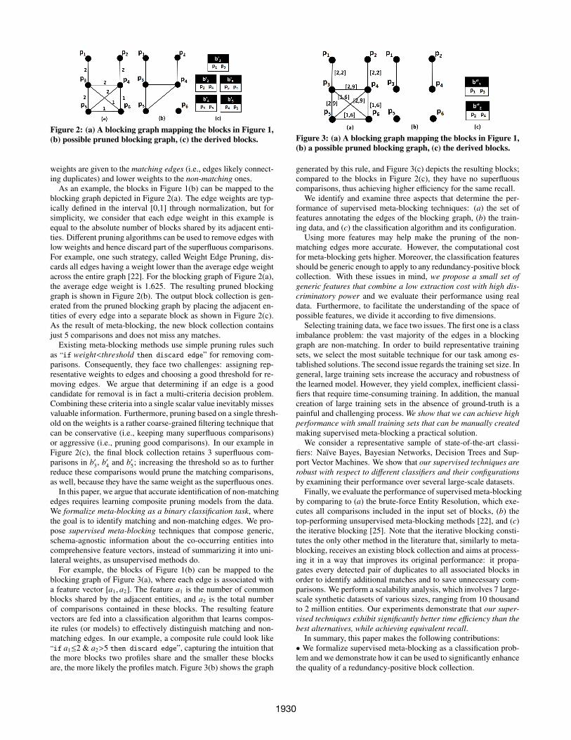
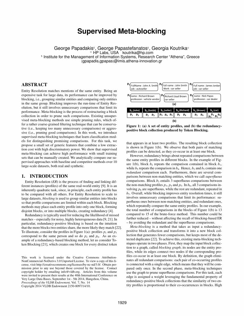
Figure 2: (a) A blocking graph mapping the blocks in Figure 1,(b) possible pruned blocking graph, (c) the derived blocks.

weights are given to the matching edges (i.e., edges likely connect-ing duplicates) and lower weights to the non-matching ones.

As an example, the blocks in Figure 1(b) can be mapped to theblocking graph depicted in Figure 2(a). The edge weights are typ-ically defined in the interval [0,1] through normalization, but forsimplicity, we consider that each edge weight in this example isequal to the absolute number of blocks shared by its adjacent enti-ties. Different pruning algorithms can be used to remove edges withlow weights and hence discard part of the superfluous comparisons.For example, one such strategy, called Weight Edge Pruning, dis-cards all edges having a weight lower than the average edge weightacross the entire graph [22]. For the blocking graph of Figure 2(a),the average edge weight is 1.625. The resulting pruned blockinggraph is shown in Figure 2(b). The output block collection is gen-erated from the pruned blocking graph by placing the adjacent en-tities of every edge into a separate block as shown in Figure 2(c).As the result of meta-blocking, the new block collection containsjust 5 comparisons and does not miss any matches.

Existing meta-blocking methods use simple pruning rules suchas “if weight<threshold then discard edge” for removing com-parisons. Consequently, they face two challenges: assigning rep-resentative weights to edges and choosing a good threshold for re-moving edges. We argue that determining if an edge is a goodcandidate for removal is in fact a multi-criteria decision problem.Combining these criteria into a single scalar value inevitably missesvaluable information. Furthermore, pruning based on a single thresh-old on the weights is a rather coarse-grained filtering technique thatcan be conservative (i.e., keeping many superfluous comparisons)or aggressive (i.e., pruning good comparisons). In our example inFigure 2(c), the final block collection retains 3 superfluous com-parisons in b′3, b′4 and b′5; increasing the threshold so as to furtherreduce these comparisons would prune the matching comparisons,as well, because they have the same weight as the superfluous ones.

In this paper, we argue that accurate identification of non-matchingedges requires learning composite pruning models from the data.We formalize meta-blocking as a binary classification task, wherethe goal is to identify matching and non-matching edges. We pro-pose supervised meta-blocking techniques that compose generic,schema-agnostic information about the co-occurring entities intocomprehensive feature vectors, instead of summarizing it into uni-lateral weights, as unsupervised methods do.

For example, the blocks of Figure 1(b) can be mapped to theblocking graph of Figure 3(a), where each edge is associated witha feature vector [a1, a2]. The feature a1 is the number of commonblocks shared by the adjacent entities, and a2 is the total numberof comparisons contained in these blocks. The resulting featurevectors are fed into a classification algorithm that learns compos-ite rules (or models) to effectively distinguish matching and non-matching edges. In our example, a composite rule could look like“if a1≤2 & a2>5 then discard edge”, capturing the intuition thatthe more blocks two profiles share and the smaller these blocksare, the more likely the profiles match. Figure 3(b) shows the graph

Figure 3: (a) A blocking graph mapping the blocks in Figure 1,(b) a possible pruned blocking graph, (c) the derived blocks.

generated by this rule, and Figure 3(c) depicts the resulting blocks;compared to the blocks in Figure 2(c), they have no superfluouscomparisons, thus achieving higher efficiency for the same recall.

We identify and examine three aspects that determine the per-formance of supervised meta-blocking techniques: (a) the set offeatures annotating the edges of the blocking graph, (b) the train-ing data, and (c) the classification algorithm and its configuration.

Using more features may help make the pruning of the non-matching edges more accurate. However, the computational costfor meta-blocking gets higher. Moreover, the classification featuresshould be generic enough to apply to any redundancy-positive blockcollection. With these issues in mind, we propose a small set ofgeneric features that combine a low extraction cost with high dis-criminatory power and we evaluate their performance using realdata. Furthermore, to facilitate the understanding of the space ofpossible features, we divide it according to five dimensions.

Selecting training data, we face two issues. The first one is a classimbalance problem: the vast majority of the edges in a blockinggraph are non-matching. In order to build representative trainingsets, we select the most suitable technique for our task among es-tablished solutions. The second issue regards the training set size. Ingeneral, large training sets increase the accuracy and robustness ofthe learned model. However, they yield complex, inefficient classi-fiers that require time-consuming training. In addition, the manualcreation of large training sets in the absence of ground-truth is apainful and challenging process. We show that we can achieve highperformance with small training sets that can be manually createdmaking supervised meta-blocking a practical solution.

We consider a representative sample of state-of-the-art classi-fiers: Naıve Bayes, Bayesian Networks, Decision Trees and Sup-port Vector Machines. We show that our supervised techniques arerobust with respect to different classifiers and their configurationsby examining their performance over several large-scale datasets.

Finally, we evaluate the performance of supervised meta-blockingby comparing to (a) the brute-force Entity Resolution, which exe-cutes all comparisons included in the input set of blocks, (b) thetop-performing unsupervised meta-blocking methods [22], and (c)the iterative blocking [25]. Note that the iterative blocking consti-tutes the only other method in the literature that, similarly to meta-blocking, receives an existing block collection and aims at process-ing it in a way that improves its original performance: it propa-gates every detected pair of duplicates to all associated blocks inorder to identify additional matches and to save unnecessary com-parisons. We perform a scalability analysis, which involves 7 large-scale synthetic datasets of various sizes, ranging from 10 thousandto 2 million entities. Our experiments demonstrate that our super-vised techniques exhibit significantly better time efficiency than thebest alternatives, while achieving equivalent recall.

In summary, this paper makes the following contributions:• We formalize supervised meta-blocking as a classification prob-lem and we demonstrate how it can be used to significantly enhancethe quality of a redundancy-positive block collection.

1930

•We map the space of possible classification features along five di-mensions and we select a small set of generic features that combinea low extraction cost with high discriminatory power. We evaluatetheir performance using real data.•We show that small training sets, which can be manually created,can achieve high performance, making supervised meta-blocking apractical solution for Entity Resolution.• We show that our supervised techniques are robust with respectto different classifiers and their configurations by examining theirperformance over several large-scale datasets.• We perform a thorough scalability analysis, comparing super-vised meta-blocking against the best competitor approaches.

The rest of the paper is structured as follows. Section 2 presentsrelated work, Section 3 provides a brief overview of unsupervisedmeta-blocking, Section 4 introduces supervised meta-blocking, andSection 5 describes the real-world datasets and the metrics used inthe evaluation. Sections 6 and 7 cover feature and training set selec-tion, while in Section 8, we fine-tune the classification algorithms.Section 9 experimentally compares supervised meta-blocking withcompetitor techniques and finally, Section 10 concludes the paper.

2. RELATED WORKThere is a large body of work on Entity Resolution [9, 19]. Block-

ing techniques group similar entities into blocks so that profilecomparisons are limited within each block. These methods can bedistinguished into schema-based and schema-agnostic ones.

Schema-based methods (e.g., Sorted Neighborhood [12], Suf-fix Array [7], HARRA [14], Canopy Clustering [17], and q-gramsblocking [10]) group entities based on knowledge about the se-mantics of their attributes. These approaches are only suitable forhomogeneous information spaces, like databases, where the qual-ity of the schema is known a-priori. In contrast, schema-agnosticblocking techniques cluster entities into blocks without requiringany knowledge about the underlying schema(ta). For instance, inToken Blocking [21], every token that is shared by at least two en-tities creates an individual block. Total Description [20] improveson Token Blocking by considering the most discriminative parts ofentity URIs instead of all their tokens. In the same category fallAttribute Clustering [21] and TYPiMatch [16]. These techniquesare preferred in the context of heterogeneous information spaces,which involve large volumes of noisy, semi-structured data that areloosely bound to various schemata [11].

Both schema-based and schema-agnostic blocking methods usu-ally produce redundancy-positive block collections [22]. Meta-blocking operates on top of them, improving the balance betweenprecision and recall by restructuring the block collection [22].

All the aforementioned approaches rely on an unsupervised func-tionality. Supervised learning has been applied to blocking-basedER with the purpose of fine-tuning the configuration of schema-based blocking methods: in [1, 18], the authors propose methodsfor learning combinations of attribute names and similarity met-rics that are suitable for extracting and comparing blocking keys.Supervised learning has also been applied to generic ER in orderto classify pairs of entities into matching and non-matching, byadapting similarity metrics and the corresponding thresholds to aparticular domain [2, 6, 8, 24]. Other works introduce methods forfacilitating the construction of the training set [23], while in [3], theauthors propose supervised techniques for combining the decisionsof multiple ER systems into an ensemble of higher performance.No prior work has applied supervised learning techniques to thetask of meta-blocking.

3. PRELIMINARIESIn this section, we introduce the main concepts and notation used

in the paper and we provide a brief overview of existing unsuper-vised meta-blocking techniques. Table 1 summarizes notation.

An entity profile p is a uniquely identified collection of informa-tion described in terms of name-value pairs. An entity collection Eis a set of entity profiles. Two profiles pi, p j ∈ E are duplicates ormatches (pi≡p j) if they represent the same real-world object.

Entity Resolution comes in two forms. Clean-Clean ER receivesas input two duplicate-free but overlapping entity collections andreturns as output all pairs of duplicate profiles they contain. DirtyER receives as input a single entity collection that contains dupli-cates in itself and returns the set of matching entity profiles. Block-ing can be used to scale both forms of ER to large entity collectionsby clustering similar profiles into blocks so that comparisons are re-stricted among the entity profiles within each block bi.

The quality of a block collection B can be measured in termsof two competing criteria, namely precision and recall, which areestimated through the following established measures [1, 7, 18, 21]:

(i) Pairs Quality (PQ) assesses precision, i.e., the portion of non-redundant comparisons between matching entities. It is defined as:PQ(B) = |D(B)|/||B||, where D(B) represents the set of detectablematches, i.e. the pairs of duplicate profiles that co-occur in at leastone block, and |D(B)| stands for its size. ||B|| is called aggregatecardinality and denotes the total number of comparisons containedin B: ||B|| =

∑bi∈B ||bi||, where ||bi|| is the cardinality of bi (i.e.,

the number of pair-wise comparisons it entails). PQ takes valuesin [0, 1], with higher values indicating higher precision for B, i.e.,fewer superfluous and redundant comparisons.

(ii) Pair Completeness (PC) assesses recall, i.e., the portion ofduplicates that share at least one block and, thus, can be detected.It is formally defined as: PC(B) = |D(B)|/|D(E)|, whereD(E) rep-resents the set of duplicates contained in the input entity collectionE, and |D(E)| stands for its size. PC values are in the interval [0, 1],with higher values indicating higher recall for B.

Note that we follow a known best practice [1, 4, 18, 25], ex-amining the quality of a block collection independently of profilematching techniques. In particular, we assume an oracle exists thatcorrectly decides whether two entity profiles match or not. Thus,D(B) is equivalent to the set of matching comparisons in B. Therationale of this approach is that a block collection with high pre-cision and high recall guarantees that the quality of a complete ERsolution is as good as that of the selected entity matching algorithm.

There is a clear trade-off between the precision and the recallof B: as more comparisons are executed (i.e., higher ||B||), its re-call increases (i.e., higher |D(B)|), but its precision decreases, andvice versa. The redundancy-positive block collections achieve highPC at the cost of lower PQ, as they place every entity profile intomultiple blocks. Meta-blocking aims at improving this balance byrestructuring a redundancy-positive block collection B into a newone B′ of higher precision but equivalent recall. More formally:

Problem 1 (Meta-blocking). Given a redundancy-positive blockcollection B, the goal of meta-blocking is to restructure B into anew collection B′ that achieves significantly higher precision, whilemaintaining the original recall (PQ(B′)�PQ(B), PC(B′)≈PC(B)).

Existing meta-blocking techniques rely their functionality on theweighted blocking graph (GB), a data structure that models theblock assignments in the block collection B. As illustrated in Fig-ure 2(a), GB is formed by creating a node for every entity profilein B and an undirected edge for every non-redundant pair of co-occurring profiles. Formally, this structure is defined as follows:

1931

pi an entity profileB, |B|, ||B|| a block collection, its size (# of blocks), its cardinality (# of comparisons)bi, |bi |, ||bi || a block, its size (# of entities), its cardinality (# of comparisons)GB, VB, EB the generalized blocking graph of B, its nodes and its edgesGvi , Vvi , Evi the neighborhood of node vi, its nodes and its edges.Bi⊆B, |Bi | the set of blocks containing pi and its size (# of blocks)Bi, j⊆B the set of blocks shared by the pi and p j (Bi, j=Bi∩B j)|Bi, j | the size of Bi, j, i.e., # of comparisons between pi and p jD(B),|D(B)| the set of detected duplicates in B and its sizepi.comp() the set of comparisons entailing pi (including the redundant ones)

Table 1: Summary of main notation.

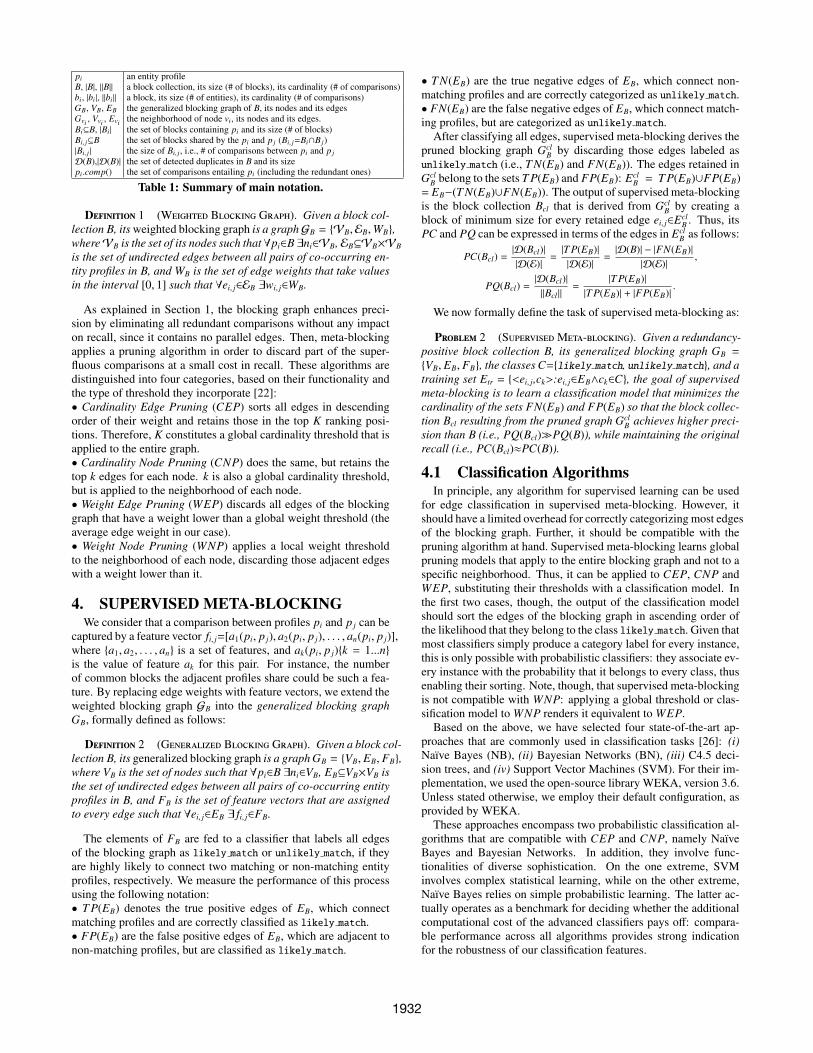
Definition 1 (Weighted Blocking Graph). Given a block col-lection B, its weighted blocking graph is a graphGB = {VB,EB,WB},whereVB is the set of its nodes such that ∀pi∈B ∃ni∈VB, EB⊆VB×VB

is the set of undirected edges between all pairs of co-occurring en-tity profiles in B, and WB is the set of edge weights that take valuesin the interval [0, 1] such that ∀ei, j∈EB ∃wi, j∈WB.

As explained in Section 1, the blocking graph enhances preci-sion by eliminating all redundant comparisons without any impacton recall, since it contains no parallel edges. Then, meta-blockingapplies a pruning algorithm in order to discard part of the super-fluous comparisons at a small cost in recall. These algorithms aredistinguished into four categories, based on their functionality andthe type of threshold they incorporate [22]:• Cardinality Edge Pruning (CEP) sorts all edges in descendingorder of their weight and retains those in the top K ranking posi-tions. Therefore, K constitutes a global cardinality threshold that isapplied to the entire graph.• Cardinality Node Pruning (CNP) does the same, but retains thetop k edges for each node. k is also a global cardinality threshold,but is applied to the neighborhood of each node.• Weight Edge Pruning (WEP) discards all edges of the blockinggraph that have a weight lower than a global weight threshold (theaverage edge weight in our case).• Weight Node Pruning (WNP) applies a local weight thresholdto the neighborhood of each node, discarding those adjacent edgeswith a weight lower than it.

4. SUPERVISED META-BLOCKINGWe consider that a comparison between profiles pi and p j can be

captured by a feature vector fi, j=[a1(pi, p j), a2(pi, p j), . . . , an(pi, p j)],where {a1, a2, . . . , an} is a set of features, and ak(pi, p j){k = 1...n}is the value of feature ak for this pair. For instance, the numberof common blocks the adjacent profiles share could be such a fea-ture. By replacing edge weights with feature vectors, we extend theweighted blocking graph GB into the generalized blocking graphGB, formally defined as follows:

Definition 2 (Generalized Blocking Graph). Given a block col-lection B, its generalized blocking graph is a graph GB = {VB, EB, FB},where VB is the set of nodes such that ∀pi∈B ∃ni∈VB, EB⊆VB×VB isthe set of undirected edges between all pairs of co-occurring entityprofiles in B, and FB is the set of feature vectors that are assignedto every edge such that ∀ei, j∈EB ∃ fi, j∈FB.

The elements of FB are fed to a classifier that labels all edgesof the blocking graph as likely match or unlikely match, if theyare highly likely to connect two matching or non-matching entityprofiles, respectively. We measure the performance of this processusing the following notation:• T P(EB) denotes the true positive edges of EB, which connectmatching profiles and are correctly classified as likely match.• FP(EB) are the false positive edges of EB, which are adjacent tonon-matching profiles, but are classified as likely match.

• T N(EB) are the true negative edges of EB, which connect non-matching profiles and are correctly categorized as unlikely match.• FN(EB) are the false negative edges of EB, which connect match-ing profiles, but are categorized as unlikely match.

After classifying all edges, supervised meta-blocking derives thepruned blocking graph Gcl

B by discarding those edges labeled asunlikely match (i.e., T N(EB) and FN(EB)). The edges retained inGcl

B belong to the sets T P(EB) and FP(EB): EclB = T P(EB)∪FP(EB)

= EB−(T N(EB)∪FN(EB)). The output of supervised meta-blockingis the block collection Bcl that is derived from Gcl

B by creating ablock of minimum size for every retained edge ei, j∈Ecl

B . Thus, itsPC and PQ can be expressed in terms of the edges in Ecl

B as follows:

PC(Bcl) =|D(Bcl)||D(E)|

=|T P(EB)||D(E)|

=|D(B)| − |FN(EB)|

|D(E)|,

PQ(Bcl) =|D(Bcl)|||Bcl ||

=|T P(EB)|

|T P(EB)| + |FP(EB)|.

We now formally define the task of supervised meta-blocking as:

Problem 2 (SupervisedMeta-blocking). Given a redundancy-positive block collection B, its generalized blocking graph GB =

{VB, EB, FB}, the classes C={likely match, unlikely match}, and atraining set Etr = {<ei, j,ck>:ei, j∈EB∧ck∈C}, the goal of supervisedmeta-blocking is to learn a classification model that minimizes thecardinality of the sets FN(EB) and FP(EB) so that the block collec-tion Bcl resulting from the pruned graph Gcl

B achieves higher preci-sion than B (i.e., PQ(Bcl)�PQ(B)), while maintaining the originalrecall (i.e., PC(Bcl)≈PC(B)).

4.1 Classification AlgorithmsIn principle, any algorithm for supervised learning can be used

for edge classification in supervised meta-blocking. However, itshould have a limited overhead for correctly categorizing most edgesof the blocking graph. Further, it should be compatible with thepruning algorithm at hand. Supervised meta-blocking learns globalpruning models that apply to the entire blocking graph and not to aspecific neighborhood. Thus, it can be applied to CEP, CNP andWEP, substituting their thresholds with a classification model. Inthe first two cases, though, the output of the classification modelshould sort the edges of the blocking graph in ascending order ofthe likelihood that they belong to the class likely match. Given thatmost classifiers simply produce a category label for every instance,this is only possible with probabilistic classifiers: they associate ev-ery instance with the probability that it belongs to every class, thusenabling their sorting. Note, though, that supervised meta-blockingis not compatible with WNP: applying a global threshold or clas-sification model to WNP renders it equivalent to WEP.

Based on the above, we have selected four state-of-the-art ap-proaches that are commonly used in classification tasks [26]: (i)Naıve Bayes (NB), (ii) Bayesian Networks (BN), (iii) C4.5 deci-sion trees, and (iv) Support Vector Machines (SVM). For their im-plementation, we used the open-source library WEKA, version 3.6.Unless stated otherwise, we employ their default configuration, asprovided by WEKA.

These approaches encompass two probabilistic classification al-gorithms that are compatible with CEP and CNP, namely NaıveBayes and Bayesian Networks. In addition, they involve func-tionalities of diverse sophistication. On the one extreme, SVMinvolves complex statistical learning, while on the other extreme,Naıve Bayes relies on simple probabilistic learning. The latter ac-tually operates as a benchmark for deciding whether the additionalcomputational cost of the advanced classifiers pays off: compara-ble performance across all algorithms provides strong indicationfor the robustness of our classification features.

1932

To solve the supervised meta-blocking problem, we need to de-termine the features to annotate the edges of the blocking graph(Section 6) and the appropriate training set, both in terms of sizeand composition (Section 7). In Section 5, we introduce the datasetsand metrics to be used for the evaluation of the proposed solution.

5. DATASETS & METRICSDatasets. We consider both Clean-Clean and Dirty ER and we

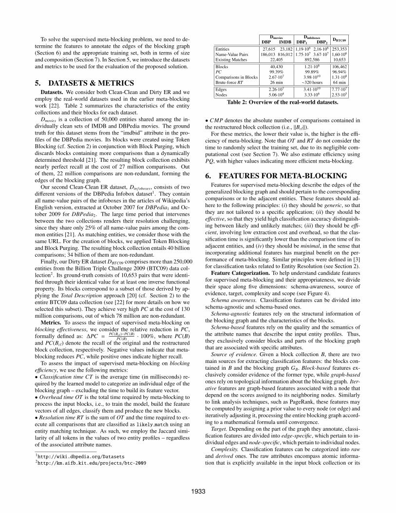
employ the real-world datasets used in the earlier meta-blockingwork [22]. Table 2 summarizes the characteristics of the entitycollections and their blocks for each dataset.

Dmovies is a collection of 50,000 entities shared among the in-dividually clean sets of IMDB and DBPedia movies. The groundtruth for this dataset stems from the “imdbid” attribute in the pro-files of the DBPedia movies. Its blocks were created using TokenBlocking (cf. Section 2) in conjunction with Block Purging, whichdiscards blocks containing more comparisons than a dynamicallydetermined threshold [21]. The resulting block collection exhibitsnearly perfect recall at the cost of 27 million comparisons. Outof them, 22 million comparisons are non-redundant, forming theedges of the blocking graph.

Our second Clean-Clean ER dataset, Din f oboxes, consists of twodifferent versions of the DBPedia Infobox dataset1. They containall name-value pairs of the infoboxes in the articles of Wikipedia’sEnglish version, extracted at October 2007 for DBPedia1 and Oc-tober 2009 for DBPedia2. The large time period that intervenesbetween the two collections renders their resolution challenging,since they share only 25% of all name-value pairs among the com-mon entities [21]. As matching entities, we consider those with thesame URL. For the creation of blocks, we applied Token Blockingand Block Purging. The resulting block collection entails 40 billioncomparisons; 34 billion of them are non-redundant.

Finally, our Dirty ER dataset DBTC09 comprises more than 250,000entities from the Billion Triple Challenge 2009 (BTC09) data col-lection2. Its ground-truth consists of 10,653 pairs that were identi-fied through their identical value for at least one inverse functionalproperty. Its blocks correspond to a subset of those derived by ap-plying the Total Description approach [20] (cf. Section 2) to theentire BTC09 data collection (see [22] for more details on how weselected this subset). They achieve very high PC at the cost of 130million comparisons, out of which 78 million are non-redundant.

Metrics. To assess the impact of supervised meta-blocking onblocking effectiveness, we consider the relative reduction in PC,formally defined as: ∆PC =

PC(Bcl)−PC(B)PC(B) · 100%, where PC(B)

and PC(Bcl) denote the recall of the original and the restructuredblock collection, respectively. Negative values indicate that meta-blocking reduces PC, while positive ones indicate higher recall.

To assess the impact of supervised meta-blocking on blockingefficiency, we use the following metrics:• Classification time CT is the average time (in milliseconds) re-quired by the learned model to categorize an individual edge of theblocking graph – excluding the time to build its feature vector.• Overhead time OT is the total time required by meta-blocking toprocess the input blocks, i.e., to train the model, build the featurevectors of all edges, classify them and produce the new blocks.• Resolution time RT is the sum of OT and the time required to ex-ecute all comparisons that are classified as likely match using anentity matching technique. As such, we employ the Jaccard simi-larity of all tokens in the values of two entity profiles – regardlessof the associated attribute names.

1http://wiki.dbpedia.org/Datasets2http://km.aifb.kit.edu/projects/btc-2009

Dmovies Dinfoboxes DBTC09DBP IMDB DBP1 DBP2

Entities 27,615 23,182 1,19·106 2,16·106 253,353Name-Value Pairs 186,013 816,012 1.75·107 3.67·107 1,60·106

Existing Matches 22,405 892,586 10,653

Blocks 40,430 1.21·106 106,462PC 99.39% 99.89% 96.94%Comparisons in Blocks 2.67·107 3.98·1010 1.31·108

Brute-force RT 26 min ∼320 hours 64 min

Edges 2.26·107 3.41·1010 7.77·107

Nodes 5.06·104 3.33·106 2.53·105

Table 2: Overview of the real-world datasets.

• CMP denotes the absolute number of comparisons contained inthe restructured block collection (i.e., ||Bcl||).

For these metrics, the lower their value is, the higher is the effi-ciency of meta-blocking. Note that OT and RT do not consider thetime to randomly select the training set, due to its negligible com-putational cost (see Section 7). We also estimate efficiency usingPQ, with higher values indicating more efficient meta-blocking.

6. FEATURES FOR META-BLOCKINGFeatures for supervised meta-blocking describe the edges of the

generalized blocking graph and should pertain to the correspondingcomparisons or to the adjacent entities. These features should ad-here to the following principles: (i) they should be generic, so thatthey are not tailored to a specific application; (ii) they should beeffective, so that they yield high classification accuracy distinguish-ing between likely and unlikely matches; (iii) they should be effi-cient, involving low extraction cost and overhead, so that the clas-sification time is significantly lower than the comparison time of itsadjacent entities, and (iv) they should be minimal, in the sense thatincorporating additional features has marginal benefit on the per-formance of meta-blocking. Similar principles were defined in [3]for classification tasks related to Entity Resolution (see Section 2).

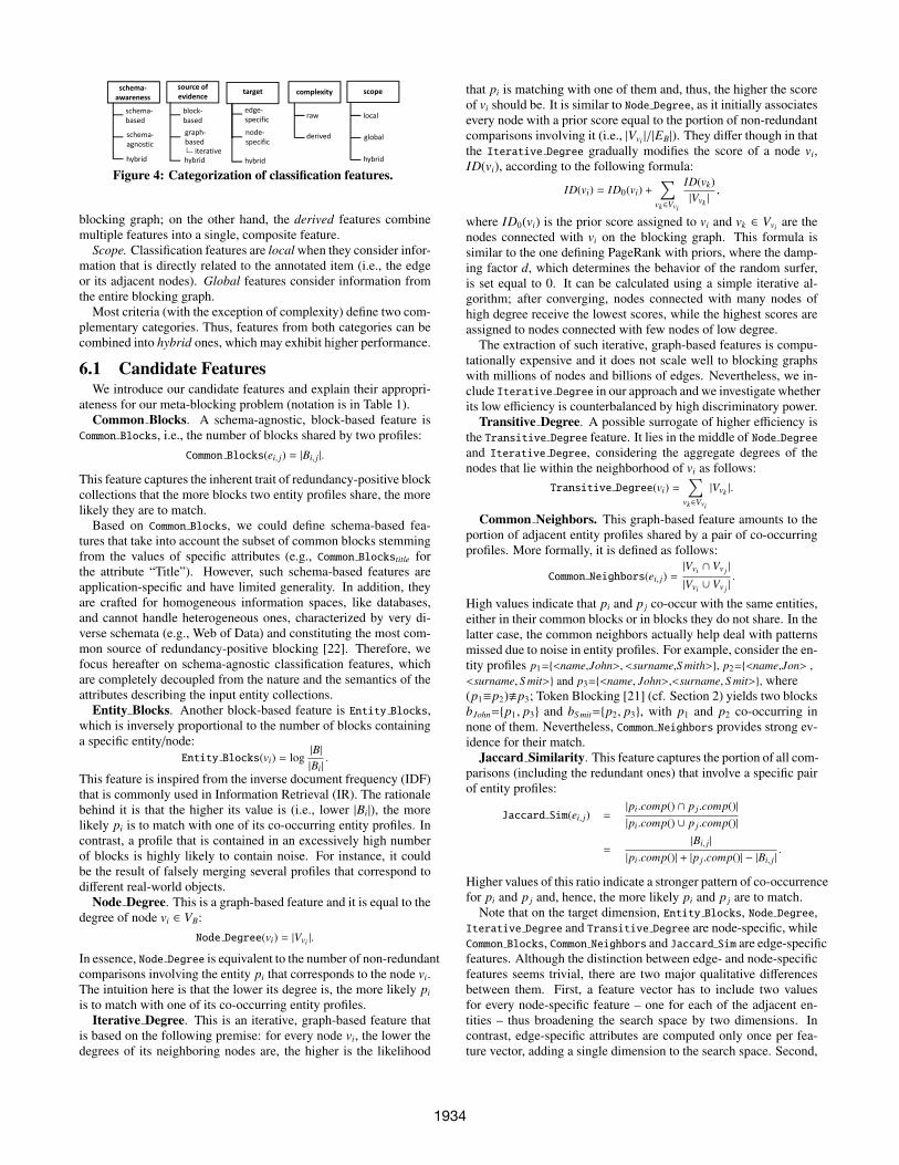
Feature Categorization. To help understand candidate featuresfor supervised meta-blocking and their appropriateness, we dividetheir space along five dimensions: schema-awareness, source ofevidence, target, complexity and scope (see Figure 4).

Schema awareness. Classification features can be divided intoschema-agnostic and schema-based ones.

Schema-agnostic features rely on the structural information ofthe blocking graph and the characteristics of the blocks.

Schema-based features rely on the quality and the semantics ofthe attribute names that describe the input entity profiles. Thus,they exclusively consider blocks and parts of the blocking graphthat are associated with specific attributes.

Source of evidence. Given a block collection B, there are twomain sources for extracting classification features: the blocks con-tained in B and the blocking graph GB. Block-based features ex-clusively consider evidence of the former type, while graph-basedones rely on topological information about the blocking graph. Iter-ative features are graph-based features associated with a node thatdepend on the scores assigned to its neighboring nodes. Similarlyto link analysis techniques, such as PageRank, these features maybe computed by assigning a prior value to every node (or edge) anditeratively adjusting it, processing the entire blocking graph accord-ing to a mathematical formula until convergence.

Target. Depending on the part of the graph they annotate, classi-fication features are divided into edge-specific, which pertain to in-dividual edges and node-specific, which pertain to individual nodes.

Complexity. Classification features can be categorized into rawand derived ones. The raw attributes encompass atomic informa-tion that is explicitly available in the input block collection or its

1933

schema‐awareness 

source of evidence  complexity target  scope 

schema‐based 

schema‐agnostic 

block‐based graph‐based 

edge‐specific 

node‐specific 

raw 

derived 

local 

global 

iterative hybrid hybrid  hybrid  hybrid 

Figure 4: Categorization of classification features.

blocking graph; on the other hand, the derived features combinemultiple features into a single, composite feature.

Scope. Classification features are local when they consider infor-mation that is directly related to the annotated item (i.e., the edgeor its adjacent nodes). Global features consider information fromthe entire blocking graph.

Most criteria (with the exception of complexity) define two com-plementary categories. Thus, features from both categories can becombined into hybrid ones, which may exhibit higher performance.

6.1 Candidate FeaturesWe introduce our candidate features and explain their appropri-

ateness for our meta-blocking problem (notation is in Table 1).Common Blocks. A schema-agnostic, block-based feature is

Common Blocks, i.e., the number of blocks shared by two profiles:Common Blocks(ei, j) = |Bi, j |.

This feature captures the inherent trait of redundancy-positive blockcollections that the more blocks two entity profiles share, the morelikely they are to match.

Based on Common Blocks, we could define schema-based fea-tures that take into account the subset of common blocks stemmingfrom the values of specific attributes (e.g., Common Blockstitle forthe attribute “Title”). However, such schema-based features areapplication-specific and have limited generality. In addition, theyare crafted for homogeneous information spaces, like databases,and cannot handle heterogeneous ones, characterized by very di-verse schemata (e.g., Web of Data) and constituting the most com-mon source of redundancy-positive blocking [22]. Therefore, wefocus hereafter on schema-agnostic classification features, whichare completely decoupled from the nature and the semantics of theattributes describing the input entity collections.

Entity Blocks. Another block-based feature is Entity Blocks,which is inversely proportional to the number of blocks containinga specific entity/node:

Entity Blocks(vi) = log|B||Bi |.

This feature is inspired from the inverse document frequency (IDF)that is commonly used in Information Retrieval (IR). The rationalebehind it is that the higher its value is (i.e., lower |Bi|), the morelikely pi is to match with one of its co-occurring entity profiles. Incontrast, a profile that is contained in an excessively high numberof blocks is highly likely to contain noise. For instance, it couldbe the result of falsely merging several profiles that correspond todifferent real-world objects.

Node Degree. This is a graph-based feature and it is equal to thedegree of node vi ∈ VB:

Node Degree(vi) = |Vvi |.

In essence, Node Degree is equivalent to the number of non-redundantcomparisons involving the entity pi that corresponds to the node vi.The intuition here is that the lower its degree is, the more likely pi

is to match with one of its co-occurring entity profiles.Iterative Degree. This is an iterative, graph-based feature that

is based on the following premise: for every node vi, the lower thedegrees of its neighboring nodes are, the higher is the likelihood

that pi is matching with one of them and, thus, the higher the scoreof vi should be. It is similar to Node Degree, as it initially associatesevery node with a prior score equal to the portion of non-redundantcomparisons involving it (i.e., |Vvi |/|EB|). They differ though in thatthe Iterative Degree gradually modifies the score of a node vi,ID(vi), according to the following formula:

ID(vi) = ID0(vi) +∑

vk∈Vvi

ID(vk)|Vvk |

,

where ID0(vi) is the prior score assigned to vi and vk ∈ Vvi are thenodes connected with vi on the blocking graph. This formula issimilar to the one defining PageRank with priors, where the damp-ing factor d, which determines the behavior of the random surfer,is set equal to 0. It can be calculated using a simple iterative al-gorithm; after converging, nodes connected with many nodes ofhigh degree receive the lowest scores, while the highest scores areassigned to nodes connected with few nodes of low degree.

The extraction of such iterative, graph-based features is compu-tationally expensive and it does not scale well to blocking graphswith millions of nodes and billions of edges. Nevertheless, we in-clude Iterative Degree in our approach and we investigate whetherits low efficiency is counterbalanced by high discriminatory power.

Transitive Degree. A possible surrogate of higher efficiency isthe Transitive Degree feature. It lies in the middle of Node Degreeand Iterative Degree, considering the aggregate degrees of thenodes that lie within the neighborhood of vi as follows:

Transitive Degree(vi) =∑

vk∈Vvi

|Vvk |.

Common Neighbors. This graph-based feature amounts to theportion of adjacent entity profiles shared by a pair of co-occurringprofiles. More formally, it is defined as follows:

Common Neighbors(ei, j) =|Vvi ∩ Vv j |

|Vvi ∪ Vv j |.

High values indicate that pi and p j co-occur with the same entities,either in their common blocks or in blocks they do not share. In thelatter case, the common neighbors actually help deal with patternsmissed due to noise in entity profiles. For example, consider the en-tity profiles p1={<name,John>, <surname,S mith>}, p2={<name,Jon> ,<surname, S mit>} and p3={<name, John>,<surname, S mit>}, where(p1≡p2).p3; Token Blocking [21] (cf. Section 2) yields two blocksbJohn={p1, p3} and bS mit={p2, p3}, with p1 and p2 co-occurring innone of them. Nevertheless, Common Neighbors provides strong ev-idence for their match.

Jaccard Similarity. This feature captures the portion of all com-parisons (including the redundant ones) that involve a specific pairof entity profiles:

Jaccard Sim(ei, j) =|pi.comp() ∩ p j.comp()||pi.comp() ∪ p j.comp()|

=|Bi, j |

|pi.comp()| + |p j.comp()| − |Bi, j |.

Higher values of this ratio indicate a stronger pattern of co-occurrencefor pi and p j and, hence, the more likely pi and p j are to match.

Note that on the target dimension, Entity Blocks, Node Degree,Iterative Degree and Transitive Degree are node-specific, whileCommon Blocks, Common Neighbors and Jaccard Sim are edge-specificfeatures. Although the distinction between edge- and node-specificfeatures seems trivial, there are two major qualitative differencesbetween them. First, a feature vector has to include two valuesfor every node-specific feature – one for each of the adjacent en-tities – thus broadening the search space by two dimensions. Incontrast, edge-specific attributes are computed only once per fea-ture vector, adding a single dimension to the search space. Second,

1934

source of evidence  target  complexity  scope 

block‐based 

graph‐based  iterative

edge‐specific 

node‐specific hybrid raw  derived  local  global  hybrid 

 CF_IBF         Jaccard_Sim           RACCB           Node_Degree                Iterative_Degree              Transitive_Degree                

Figure 5: Categorization of the features of our approach.

edge-specific features are expected to exhibit higher discriminatorypower than the node-specific ones, because every value of the latterparticipates in as many feature vectors as the degree of the corre-sponding node; in contrast, every value of the edge-specific featurespertains to a single feature vector.

(Reciprocal) Aggregate Cardinality of Common Blocks. Fromthe aforementioned features, only Common Blocks and Node Degreeare raw. In general, there is no rule-of-thumb for a-priori determin-ing which form of features achieves the best performance in prac-tice. Even different forms of derived features may lead to signifi-cant differences in classification accuracy. As an example, considertwo edge-specific features that use the same information, but in dif-ferent forms: the Aggregate Cardinality of Common Blocks (ACCB)and the Reciprocal Aggregate Cardinality of Common Blocks (RACCB)attributes. The former sums the cardinalities of the blocks sharedby the adjacent entities (raw feature): ACCB(ei, j) =

∑bk∈Bi, j

||bk ||.The latter sums the inverse of the cardinalities of common blocks(derived feature):

RACCB(ei, j) =∑

bk∈Bi, j

1||bk ||.

Both features rely on the premise that the smaller the blocks twoentities co-occur in, the more likely they are to be matching. Hence,the lower the value of ACCB is, the more likely the co-occurring en-tities match, and vice versa for RACCB. Preliminary experiments,though, demonstrated that ACCB achieves significantly lower classi-fication accuracy than RACCB, due to its low discriminativeness: itassigns identical or similar values to pairs of co-occurring entitiesthat share blocks of totally different cardinalities. For instance, con-sider two pairs of entities: the first co-occurs in 3 blocks containing1,2 and 4 comparisons, while the second shares 2 blocks with 2 and5 comparisons; ACCB takes the same value for both edges (7), whileRACCB amounts to 1.75 and 0.70 for the first and the second pair,respectively, favoring the entities that are more likely to match.

Co-occurrence Frequency-Inverse Block Frequency. Derivedfeatures can come in more advanced forms than RACCB, combiningmultiple features through linear or non-linear functions. However,they should be used with caution for several reasons: (i) they in-volve a higher extraction cost than the comprising raw features; (ii)their form might be too complex to be interpretable; (iii) they areusually correlated with the raw features they comprise and, thus,are incompatible with them, when applied to classifiers with strongindependence assumptions (e.g., Naıve Bayes); (iv) some classi-fication algorithms may operate better with raw features, learningthemselves the linear or non-linear associations between the inputfeatures. For these reasons, the derived features should involve alow extraction cost and transform as few raw features as possible.

Here, we combine Common Blocks and Entity Blocks into a fea-ture inspired from the TF-IDF measure employed in IR. We callit Co-occurrence Frequency-Inverse Block Frequency (CF IBF)and formally define it as:

CF IBF(ei, j) = |Bi, j | · log|B||Bi |· log

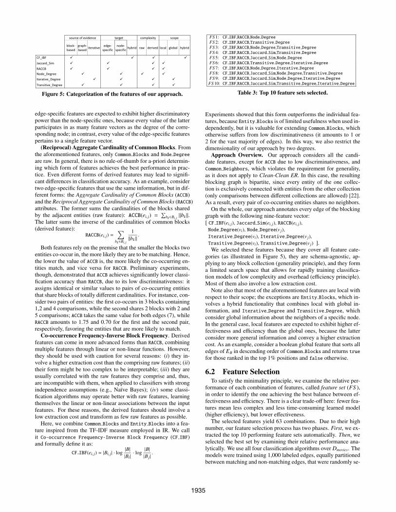
|B||B j |.

FS 1: CF IBF,RACCB,Node DegreeFS 2: CF IBF,RACCB,Transitive DegreeFS 3: CF IBF,RACCB,Node Degree,Transitive DegreeFS 4: CF IBF,RACCB,Jaccard Sim,Transitive DegreeFS 5: CF IBF,RACCB,Jaccard Sim,Node DegreeFS 6: CF IBF,RACCB,Transitive Degree,Iterative DegreeFS 7: CF IBF,RACCB,Node Degree,Iterative DegreeFS 8: CF IBF,RACCB,Jaccard Sim,Node Degree,Transitive DegreeFS 9: CF IBF,RACCB,Jaccard Sim,Node Degree,Iterative DegreeFS 10: CF IBF,RACCB,Jaccard Sim,Transitive Degree,Iterative Degree

Table 3: Top 10 feature sets selected.

Experiments showed that this form outperforms the individual fea-tures, because Entity Blocks is of limited usefulness when used in-dependently, but it is valuable for extending Common Blocks, whichotherwise suffers from low discriminativeness (it amounts to 1 or2 for the vast majority of edges). In this way, we also restrict thedimensionality of our approach by two degrees.

Approach Overview. Our approach considers all the candi-date features, except for ACCB due to low discriminativeness, andCommon Neighbors, which violates the requirement for generality,as it does not apply to Clean-Clean ER. In this case, the resultingblocking graph is bipartite, since every entity of the one collec-tion is exclusively connected with entities from the other collection(only comparisons between different collections are allowed) [22].As a result, every pair of co-occurring entities shares no neighbors.

On the whole, our approach annotates every edge of the blockinggraph with the following nine-feature vector:[ CF IBF(ei, j), Jaccard Sim(ei, j), RACCB(ei, j),Node Degree(vi), Node Degree(v j),Iterative Degree(vi), Iterative Degree(v j),Trasitive Degree(vi), Transitive Degree(v j) ].We selected these features because they cover all feature cate-

gories (as illustrated in Figure 5), they are schema-agnostic, ap-plying to any block collection (generality principle), and they forma limited search space that allows for rapidly training classifica-tion models of low complexity and overhead (efficiency principle).Most of them also involve a low extraction cost.

Note also that most of the aforementioned features are local withrespect to their scope; the exceptions are Entity Blocks, which in-volves a hybrid functionality that combines local with global in-formation, and Iterative Degree and Transitive Degree, whichconsider global information about the neighbors of a specific node.In the general case, local features are expected to exhibit higher ef-fectiveness and efficiency than the global ones, because the latterconsider more general information and convey a higher extractioncost. As an example, consider a boolean global feature that sorts alledges of EB in descending order of Common Blocks and returns truefor those ranked in the top 1% positions and false otherwise.

6.2 Feature SelectionTo satisfy the minimality principle, we examine the relative per-

formance of each combination of features, called feature set (FS ),in order to identify the one achieving the best balance between ef-fectiveness and efficiency. There is a clear trade-off here: fewer fea-tures mean less complex and less time-consuming learned model(higher efficiency), but lower effectiveness.

The selected features yield 63 combinations. Due to their highnumber, our feature selection process has two phases. First, we ex-tracted the top 10 performing feature sets automatically. Then, weselected the best set by examining their relative performance ana-lytically. We use all four classification algorithms over Dmovies. Themodels were trained using 1,000 labeled edges, equally partitionedbetween matching and non-matching edges, that were randomly se-

1935

‐10

‐8

‐6

‐4

‐2FS1 FS2 FS3 FS4 FS5 FS6 FS7 FS8 FS9 FS10

ΔPC (%) 

Naïve Bayes C4.5 SVM Bayes Networks

(a)‐10

‐9

‐8

‐7

‐6

‐5

‐4

‐3

‐2FS1 FS2 FS3 FS4 FS5 FS6 FS7 FS8 FS9 FS10

ΔPC (%) 

(a)

200,000

400,000

600,000

800,000

1,000,000

FS1 FS2 FS3 FS4 FS5 FS6 FS7 FS8 FS9 FS10

CMP (compar.) 

(b) 

0.00

0.02

0.04

0.06

0.08

0.10

0.12

FS1 FS2 FS3 FS4 FS5 FS6 FS7 FS8 FS9 FS10

CT (msec) 

(c) 

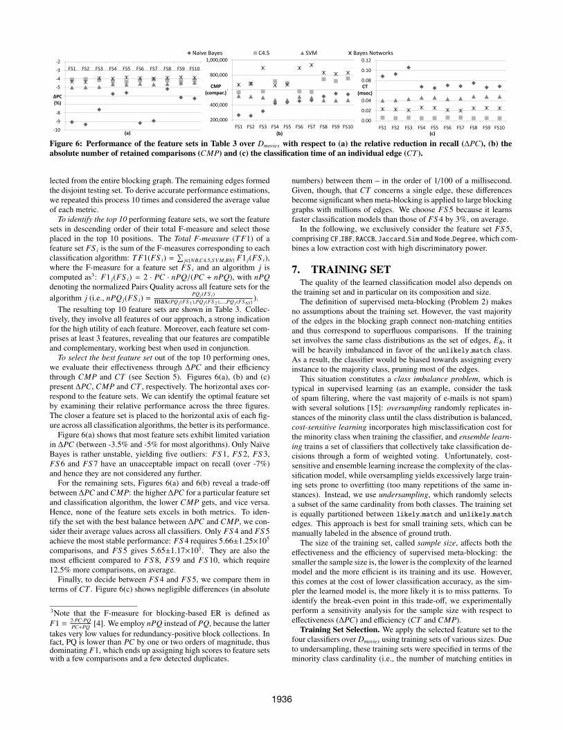
Figure 6: Performance of the feature sets in Table 3 over Dmovies with respect to (a) the relative reduction in recall (∆PC), (b) theabsolute number of retained comparisons (CMP) and (c) the classification time of an individual edge (CT ).

lected from the entire blocking graph. The remaining edges formedthe disjoint testing set. To derive accurate performance estimations,we repeated this process 10 times and considered the average valueof each metric.

To identify the top 10 performing feature sets, we sort the featuresets in descending order of their total F-measure and select thoseplaced in the top 10 positions. The Total F-measure (T F1) of afeature set FS i is the sum of the F-measures corresponding to eachclassification algorithm: T F1(FS i) =

∑j∈{NB,C4.5,S V M,BN} F1 j(FS i),

where the F-measure for a feature set FS i and an algorithm j iscomputed as3: F1 j(FS i) = 2 · PC · nPQ/(PC + nPQ), with nPQdenoting the normalized Pairs Quality across all feature sets for thealgorithm j (i.e., nPQ j(FS i) =

PQ j(FS i)max(PQ j(FS 1),PQ j(FS 2),...,PQ j(FS 63) ).

The resulting top 10 feature sets are shown in Table 3. Collec-tively, they involve all features of our approach, a strong indicationfor the high utility of each feature. Moreover, each feature set com-prises at least 3 features, revealing that our features are compatibleand complementary, working best when used in conjunction.

To select the best feature set out of the top 10 performing ones,we evaluate their effectiveness through ∆PC and their efficiencythrough CMP and CT (see Section 5). Figures 6(a), (b) and (c)present ∆PC, CMP and CT , respectively. The horizontal axes cor-respond to the feature sets. We can identify the optimal feature setby examining their relative performance across the three figures.The closer a feature set is placed to the horizontal axis of each fig-ure across all classification algorithms, the better is its performance.

Figure 6(a) shows that most feature sets exhibit limited variationin ∆PC (between -3.5% and -5% for most algorithms). Only NaıveBayes is rather unstable, yielding five outliers: FS 1, FS 2, FS 3,FS 6 and FS 7 have an unacceptable impact on recall (over -7%)and hence they are not considered any further.

For the remaining sets, Figures 6(a) and 6(b) reveal a trade-off

between ∆PC and CMP: the higher ∆PC for a particular feature setand classification algorithm, the lower CMP gets, and vice versa.Hence, none of the feature sets excels in both metrics. To iden-tify the set with the best balance between ∆PC and CMP, we con-sider their average values across all classifiers. Only FS 4 and FS 5achieve the most stable performance: FS 4 requires 5.66±1.25×105

comparisons, and FS 5 gives 5.65±1.17×105. They are also themost efficient compared to FS 8, FS 9 and FS 10, which require12.5% more comparisons, on average.

Finally, to decide between FS 4 and FS 5, we compare them interms of CT . Figure 6(c) shows negligible differences (in absolute

3Note that the F-measure for blocking-based ER is defined asF1 =

2·PC·PQPC+PQ [4]. We employ nPQ instead of PQ, because the latter

takes very low values for redundancy-positive block collections. Infact, PQ is lower than PC by one or two orders of magnitude, thusdominating F1, which ends up assigning high scores to feature setswith a few comparisons and a few detected duplicates.

numbers) between them – in the order of 1/100 of a millisecond.Given, though, that CT concerns a single edge, these differencesbecome significant when meta-blocking is applied to large blockinggraphs with millions of edges. We choose FS 5 because it learnsfaster classification models than those of FS 4 by 3%, on average.

In the following, we exclusively consider the feature set FS 5,comprising CF IBF, RACCB, Jaccard Sim and Node Degree, which com-bines a low extraction cost with high discriminatory power.

7. TRAINING SETThe quality of the learned classification model also depends on

the training set and in particular on its composition and size.The definition of supervised meta-blocking (Problem 2) makes

no assumptions about the training set. However, the vast majorityof the edges in the blocking graph connect non-matching entitiesand thus correspond to superfluous comparisons. If the trainingset involves the same class distributions as the set of edges, EB, itwill be heavily imbalanced in favor of the unlikely match class.As a result, the classifier would be biased towards assigning everyinstance to the majority class, pruning most of the edges.

This situation constitutes a class imbalance problem, which istypical in supervised learning (as an example, consider the taskof spam filtering, where the vast majority of e-mails is not spam)with several solutions [15]: oversampling randomly replicates in-stances of the minority class until the class distribution is balanced,cost-sensitive learning incorporates high misclassification cost forthe minority class when training the classifier, and ensemble learn-ing trains a set of classifiers that collectively take classification de-cisions through a form of weighted voting. Unfortunately, cost-sensitive and ensemble learning increase the complexity of the clas-sification model, while oversampling yields excessively large train-ing sets prone to overfitting (too many repetitions of the same in-stances). Instead, we use undersampling, which randomly selectsa subset of the same cardinality from both classes. The training setis equally partitioned between likely match and unlikely matchedges. This approach is best for small training sets, which can bemanually labeled in the absence of ground truth.

The size of the training set, called sample size, affects both theeffectiveness and the efficiency of supervised meta-blocking: thesmaller the sample size is, the lower is the complexity of the learnedmodel and the more efficient is its training and its use. However,this comes at the cost of lower classification accuracy, as the sim-pler the learned model is, the more likely it is to miss patterns. Toidentify the break-even point in this trade-off, we experimentallyperform a sensitivity analysis for the sample size with respect toeffectiveness (∆PC) and efficiency (CT and CMP).

Training Set Selection. We apply the selected feature set to thefour classifiers over Dmovies using training sets of various sizes. Dueto undersampling, these training sets were specified in terms of theminority class cardinality (i.e., the number of matching entities in

1936

‐6.0

‐5.5

‐5.0

‐4.5

‐4.0

‐3.5

‐3.0

0.5 1.5 2.5 3.5 4.5 5.5 6.5 7.5 8.5 9.5

ΔPC (%)  

Naïve Bayes C4.5 SVM Bayesian Networks

(a)

‐6.0

‐5.5

‐5.0

‐4.5

‐4.0

‐3.5

‐3.0

0.5% 1.5% 2.5% 3.5% 4.5% 5.5% 6.5% 7.5% 8.5% 9.5%

ΔPC (%) 

(a)

sample size 

400,000

500,000

600,000

700,000

800,000

900,000

1,000,000

0.5% 1.5% 2.5% 3.5% 4.5% 5.5% 6.5% 7.5% 8.5% 9.5%

CMP  (compar.) 

      (b) sample size 

0.00

0.01

0.02

0.03

0.04

0.05

0.06

0.07

0.5% 1.5% 2.5% 3.5% 4.5% 5.5% 6.5% 7.5% 8.5% 9.5%

CT  (msec.) 

(c) sample size 

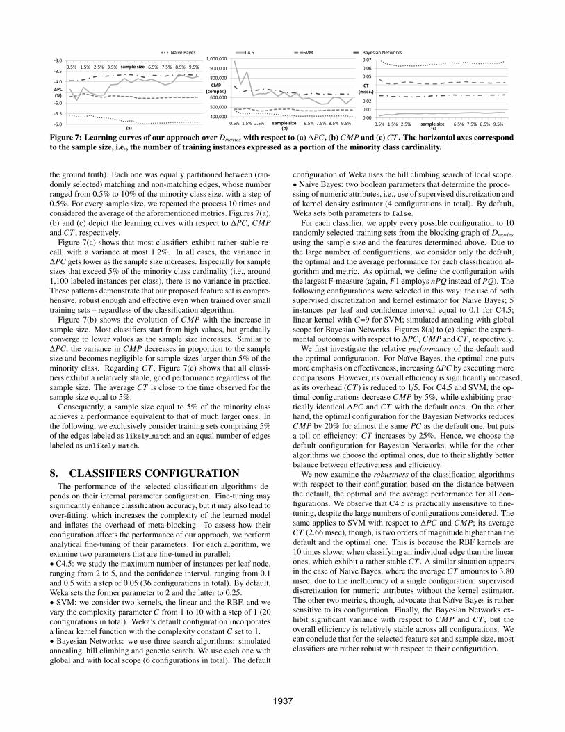
Figure 7: Learning curves of our approach over Dmovies with respect to (a) ∆PC, (b) CMP and (c) CT . The horizontal axes correspondto the sample size, i.e., the number of training instances expressed as a portion of the minority class cardinality.

the ground truth). Each one was equally partitioned between (ran-domly selected) matching and non-matching edges, whose numberranged from 0.5% to 10% of the minority class size, with a step of0.5%. For every sample size, we repeated the process 10 times andconsidered the average of the aforementioned metrics. Figures 7(a),(b) and (c) depict the learning curves with respect to ∆PC, CMPand CT , respectively.

Figure 7(a) shows that most classifiers exhibit rather stable re-call, with a variance at most 1.2%. In all cases, the variance in∆PC gets lower as the sample size increases. Especially for samplesizes that exceed 5% of the minority class cardinality (i.e., around1,100 labeled instances per class), there is no variance in practice.These patterns demonstrate that our proposed feature set is compre-hensive, robust enough and effective even when trained over smalltraining sets – regardless of the classification algorithm.

Figure 7(b) shows the evolution of CMP with the increase insample size. Most classifiers start from high values, but graduallyconverge to lower values as the sample size increases. Similar to∆PC, the variance in CMP decreases in proportion to the samplesize and becomes negligible for sample sizes larger than 5% of theminority class. Regarding CT , Figure 7(c) shows that all classi-fiers exhibit a relatively stable, good performance regardless of thesample size. The average CT is close to the time observed for thesample size equal to 5%.

Consequently, a sample size equal to 5% of the minority classachieves a performance equivalent to that of much larger ones. Inthe following, we exclusively consider training sets comprising 5%of the edges labeled as likely match and an equal number of edgeslabeled as unlikely match.

8. CLASSIFIERS CONFIGURATIONThe performance of the selected classification algorithms de-

pends on their internal parameter configuration. Fine-tuning maysignificantly enhance classification accuracy, but it may also lead toover-fitting, which increases the complexity of the learned modeland inflates the overhead of meta-blocking. To assess how theirconfiguration affects the performance of our approach, we performanalytical fine-tuning of their parameters. For each algorithm, weexamine two parameters that are fine-tuned in parallel:• C4.5: we study the maximum number of instances per leaf node,ranging from 2 to 5, and the confidence interval, ranging from 0.1and 0.5 with a step of 0.05 (36 configurations in total). By default,Weka sets the former parameter to 2 and the latter to 0.25.• SVM: we consider two kernels, the linear and the RBF, and wevary the complexity parameter C from 1 to 10 with a step of 1 (20configurations in total). Weka’s default configuration incorporatesa linear kernel function with the complexity constant C set to 1.• Bayesian Networks: we use three search algorithms: simulatedannealing, hill climbing and genetic search. We use each one withglobal and with local scope (6 configurations in total). The default

configuration of Weka uses the hill climbing search of local scope.• Naıve Bayes: two boolean parameters that determine the proce-ssing of numeric attributes, i.e., use of supervised discretization andof kernel density estimator (4 configurations in total). By default,Weka sets both parameters to false.

For each classifier, we apply every possible configuration to 10randomly selected training sets from the blocking graph of Dmovies

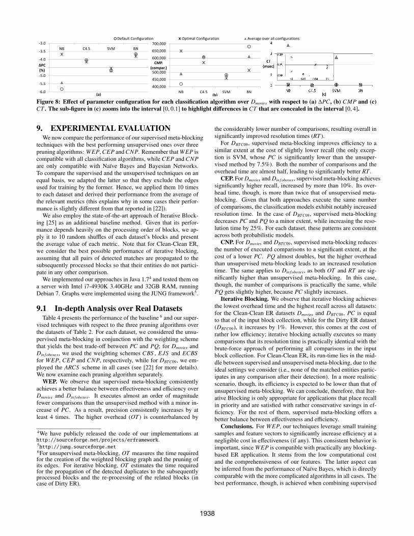
using the sample size and the features determined above. Due tothe large number of configurations, we consider only the default,the optimal and the average performance for each classification al-gorithm and metric. As optimal, we define the configuration withthe largest F-measure (again, F1 employs nPQ instead of PQ). Thefollowing configurations were selected in this way: the use of bothsupervised discretization and kernel estimator for Naive Bayes; 5instances per leaf and confidence interval equal to 0.1 for C4.5;linear kernel with C=9 for SVM; simulated annealing with globalscope for Bayesian Networks. Figures 8(a) to (c) depict the experi-mental outcomes with respect to ∆PC, CMP and CT , respectively.

We first investigate the relative performance of the default andthe optimal configuration. For Naıve Bayes, the optimal one putsmore emphasis on effectiveness, increasing ∆PC by executing morecomparisons. However, its overall efficiency is significantly increased,as its overhead (CT ) is reduced to 1/5. For C4.5 and SVM, the op-timal configurations decrease CMP by 5%, while exhibiting prac-tically identical ∆PC and CT with the default ones. On the otherhand, the optimal configuration for the Bayesian Networks reducesCMP by 20% for almost the same PC as the default one, but putsa toll on efficiency: CT increases by 25%. Hence, we choose thedefault configuration for Bayesian Networks, while for the otheralgorithms we choose the optimal ones, due to their slightly betterbalance between effectiveness and efficiency.

We now examine the robustness of the classification algorithmswith respect to their configuration based on the distance betweenthe default, the optimal and the average performance for all con-figurations. We observe that C4.5 is practically insensitive to fine-tuning, despite the large numbers of configurations considered. Thesame applies to SVM with respect to ∆PC and CMP; its averageCT (2.66 msec), though, is two orders of magnitude higher than thedefault and the optimal one. This is because the RBF kernels are10 times slower when classifying an individual edge than the linearones, which exhibit a rather stable CT . A similar situation appearsin the case of Naıve Bayes, where the average CT amounts to 3.80msec, due to the inefficiency of a single configuration: superviseddiscretization for numeric attributes without the kernel estimator.The other two metrics, though, advocate that Naıve Bayes is rathersensitive to its configuration. Finally, the Bayesian Networks ex-hibit significant variance with respect to CMP and CT , but theoverall efficiency is relatively stable across all configurations. Wecan conclude that for the selected feature set and sample size, mostclassifiers are rather robust with respect to their configuration.

1937

‐6

‐4

‐2

0NB C4.5 SVM BN

ΔPC  (%) 

Default Configuration Optimal Configuration Average over all configurations

(a)

‐6.0

‐5.5

‐5.0

‐4.5

‐4.0

‐3.5

‐3.0NB C4.5 SVM BN

ΔPC  (%) 

(a) 

400,000

450,000

500,000

550,000

600,000

650,000

700,000

NB C4.5 SVM BN

CMP.  (compar.) 

(b)

Figure 8: Effect of parameter configuration for each classification algorithm over Dmovies with respect to (a) ∆PC, (b) CMP and (c)CT . The sub-figure in (c) zooms into the interval [0, 0.1] to highlight differences in CT that are concealed in the interval [0, 4].

9. EXPERIMENTAL EVALUATIONWe now compare the performance of our supervised meta-blocking

techniques with the best performing unsupervised ones over threepruning algorithms: WEP, CEP and CNP. Remember that WEP iscompatible with all classification algorithms, while CEP and CNPare only compatible with Naıve Bayes and Bayesian Networks.To compare the supervised and the unsupervised techniques on anequal basis, we adapted the latter so that they exclude the edgesused for training by the former. Hence, we applied them 10 timesto each dataset and derived their performance from the average ofthe relevant metrics (this explains why in some cases their perfor-mance is slightly different from that reported in [22]).

We also employ the state-of-the-art approach of Iterative Block-ing [25] as an additional baseline method. Given that its perfor-mance depends heavily on the processing order of blocks, we ap-ply it to 10 random shuffles of each dataset’s blocks and presentthe average value of each metric. Note that for Clean-Clean ER,we consider the best possible performance of iterative blocking,assuming that all pairs of detected matches are propagated to thesubsequently processed blocks so that their entities do not partici-pate in any other comparison.

We implemented our approaches in Java 1.74 and tested them ona server with Intel i7-4930K 3.40GHz and 32GB RAM, runningDebian 7. Graphs were implemented using the JUNG framework5.

9.1 In-depth Analysis over Real DatasetsTable 4 presents the performance of the baseline 6 and our super-

vised techniques with respect to the three pruning algorithms overthe datasets of Table 2. For each dataset, we considered the unsu-pervised meta-blocking in conjunction with the weighting schemethat yields the best trade-off between PC and PQ; for Dmovies andDin f oboxes, we used the weighting schemes CBS , EJS and ECBSfor WEP, CEP and CNP, respectively, while for DBTC09, we em-ployed the ARCS scheme in all cases (see [22] for more details).We now examine each pruning algorithm separately.

WEP. We observe that supervised meta-blocking consistentlyachieves a better balance between effectiveness and efficiency overDmovies and Din f oboxes. It executes almost an order of magnitudefewer comparisons than the unsupervised method with a minor in-crease of PC. As a result, precision consistently increases by atleast 4 times. The higher overhead (OT ) is counterbalanced by

4We have publicly released the code of our implementations athttp://sourceforge.net/projects/erframework.5http://jung.sourceforge.net6For unsupervised meta-blocking, OT measures the time requiredfor the creation of the weighted blocking graph and the pruning ofits edges. For iterative blocking, OT estimates the time requiredfor the propagation of the detected duplicates to the subsequentlyprocessed blocks and the re-processing of the related blocks (incase of Dirty ER).

the considerably lower number of comparisons, resulting overall insignificantly improved resolution times (RT ).

For DBTC09, supervised meta-blocking improves efficiency to asimilar extent at the cost of slightly lower recall (the only excep-tion is SVM, whose PC is significantly lower than the unsuper-vised method by 7.5%). Both the number of comparisons and theoverhead time are almost half, leading to significantly better RT .

CEP. For Dmovies and Din f oboxes, supervised meta-blocking achievessignificantly higher recall, increased by more than 10%. Its over-head time, though, is more than twice that of unsupervised meta-blocking. Given that both approaches execute the same numberof comparisons, the classification models exhibit notably increasedresolution time. In the case of DBTC09, supervised meta-blockingdecreases PC and PQ to a minor extent, while increasing the reso-lution time by 25%. For each dataset, these patterns are consistentacross both probabilistic models.

CNP. For Dmovies and DBTC09, supervised meta-blocking reducesthe number of executed comparisons to a significant extent, at thecost of a lower PC. PQ almost doubles, but the higher overheadthan unsupervised meta-blocking leads to an increased resolutiontime. The same applies to Din f oboxes, as both OT and RT are sig-nificantly higher than unsupervised meta-blocking. In this case,though, the number of comparisons is practically the same, whilePQ gets slightly higher, because PC slightly increases.

Iterative Blocking. We observe that iterative blocking achievesthe lowest overhead time and the highest recall across all datasets:for the Clean-Clean ER datasets Dmovies and DBTC09, PC is equalto that of the input block collection, while for the Dirty ER dataset(DBTC09), it increases by 1%. However, this comes at the cost ofrather low efficiency; iterative blocking actually executes so manycomparisons that its resolution time is practically identical with thebrute-force approach of performing all comparisons in the inputblock collection. For Clean-Clean ER, its run-time lies in the mid-dle between supervised and unsupervised meta-blocking, due to theideal settings we consider (i.e., none of the matched entities partic-ipates in any comparison after their detection). In a more realisticscenario, though, its efficiency is expected to be lower than that ofunsupervised meta-blocking. We can conclude, therefore, that Iter-ative Blocking is only appropriate for applications that place recallin priority and are satisfied with rather conservative savings in ef-ficiency. For the rest of them, supervised meta-blocking offers abetter balance between effectiveness and efficiency.

Conclusions. For WEP, our techniques leverage small trainingsamples and feature vectors to significantly increase efficiency at anegligible cost in effectiveness (if any). This consistent behavior isimportant, since WEP is compatible with practically any blocking-based ER application. It stems from the low computational costand the comprehensiveness of our features. The latter aspect canbe inferred from the performance of Naıve Bayes, which is directlycomparable with the more complicated algorithms in all cases. Thebest performance, though, is achieved when combining supervised

1938

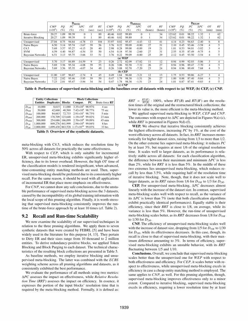
Dmovies Dinfoboxes DBTC09CMP PQ PC ∆PC OT RT CMP PQ PC ∆PC OT RT CMP PQ PC ∆PC OT RT(×105) (%) (%) (%) (sec) (sec) (×108) (%) (%) (%) (hours) (hours) (×106) (%) (%) (%) (min) (min)

Brute-force 20.27 1.09 99.39 0 1 89 40.46 0.02 99.89 0 1 34 123.62 0.01 98.22 1.32 1 62Iterative Blocking 20.27 1.09 99.39 0 1 89 40.46 0.02 99.89 0 1 34 123.62 0.01 98.22 1.32 1 62

Unsupervised 27.04 0.75 94.64 -4.78 13 104 33.97 0.02 95.47 -4.43 12 41 4.14 0.23 94.63 -2.40 6 8Naive Bayes 6.50 3.14 95.74 -3.67 39 56 3.76 0.22 99.09 -0.80 27 31 2.10 0.45 93.46 -3.58 4 5C4.5 5.69 3.57 95.27 -4.15 20 40 2.98 0.28 99.00 -0.89 19 21 1.81 0.53 94.01 -3.02 3 4SVM 4.59 4.40 94.87 -4.54 35 50 4.54 0.18 97.30 -2.60 27 31 2.55 0.35 87.49 -9.75 4 5Bayesian Networks 6.51 3.13 95.75 -3.66 33 51 3.76 0.22 99.09 -0.80 25 29 2.12 0.45 93.50 -3.54 4 5

(a) WEPUnsupervised 5.70 3.17 84.89 -14.59 9 23 0.26 2.72 82.09 -17.82 11 12 0.94 0.99 92.03 -5.06 3 4Naive Bayes 5.69 3.56 95.34 -4.08 39 55 0.26 3.06 92.58 -7.32 26 27 0.94 0.96 89.47 -7.70 4 5Bayesian Networks 5.69 3.56 95.35 -4.07 34 49 0.26 3.08 92.70 -7.20 23 24 0.94 0.96 89.49 7.68 4 5

(b) CEPUnsupervised 11.00 1.87 96.67 -2.74 8 45 0.49 1.64 96.68 -3.21 12 13 1.75 0.53 90.86 -6.27 3 4Naive Bayes 7.22 2.82 95.46 -3.95 39 59 0.47 1.79 98.38 -1.51 26 27 1.00 0.88 87.40 -9.84 4 5Bayesian Networks 7.23 2.81 95.47 -3.94 34 54 0.47 1.78 98.38 -1.51 23 24 1.01 0.87 87.41 -9.83 4 5

(c) CNPTable 4: Performance of supervised meta-blocking and the baselines over all datasets with respect to (a) WEP, (b) CEP, (c) CNP.

Entity Collections Block CollectionsEntities Duplicates Blocks Compar. PC Brute-force RT

D10K 10,000 8,615 11,088 3.35×105 98.97% 4 secD50K 50,000 42,668 40,569 7.42×106 98.77% 75 secD100K 100,000 84,663 72,733 2.91×107 98.73% 5 minD200K 200,000 170,709 123,648 1.19×108 99.02% 23 minD300K 300,000 254,686 166,099 2.70×108 99.09% 45 minD1M 1,000,000 849,276 441,999 2.94×109 99.04% 8 hrsD2M 2,000,000 1,699,430 863,528 1.17×1010 99.03% 33 hrs

Table 5: Overview of the synthetic datasets.

meta-blocking with C4.5, which reduces the resolution time by50% across all datasets for practically the same effectiveness.

With respect to CEP, which is only suitable for incrementalER, unsupervised meta-blocking exhibits significantly higher ef-ficiency, due to its lower overhead. However, the high OT time ofthe classification models is rendered insignificant, when advanced,time-consuming entity matching methods are used. Then, super-vised meta-blocking should be preferred due to its consistently higherrecall. For the same reason, it should be used with all applicationsof incremental ER that place more emphasis on effectiveness.

For CNP, we cannot draw any safe conclusions, due to the unsta-ble performance of supervised meta-blocking across the 3 datasets,caused by the incompatibility of its global training information withthe local scope of this pruning algorithm. Finally, it is worth stress-ing that supervised meta-blocking consistently improves the run-time of the brute-force approach by at least 10 times (cf. Table 2).

9.2 Recall and Run-time ScalabilityWe now examine the scalability of our supervised techniques in

relation to the three pruning algorithms. We apply them to sevensynthetic datasets that were created by FEBRL [5] and have beenwidely used in the literature for this purpose [4, 13]. They pertainto Dirty ER and their sizes range from 10 thousand to 2 millionentities. To derive redundancy-positive blocks, we applied TokenBlocking and Block Purging to each dataset. The technical charac-teristics of the resulting block collections are presented in Table 5.

As baseline methods, we employ iterative blocking and unsu-pervised meta-blocking. The latter was combined with the ECBSweighting scheme across all pruning algorithms and datasets, as itconsistently exhibited the best performance.

We evaluate the performance of all methods using two metrics:∆PC assesses the impact on effectiveness, while Relative Resolu-tion Time (RRT ) assesses the impact on efficiency. In essence, itexpresses the portion of the input blocks’ resolution time that isrequired by the meta-blocking method. Formally, it is defined as:

RRT =RT (B′)RT (B) · 100%, where RT (B) and RT (B′) are the resolu-

tion times of the original and the restructured block collections; thelower its value is, the more efficient is the meta-blocking method.

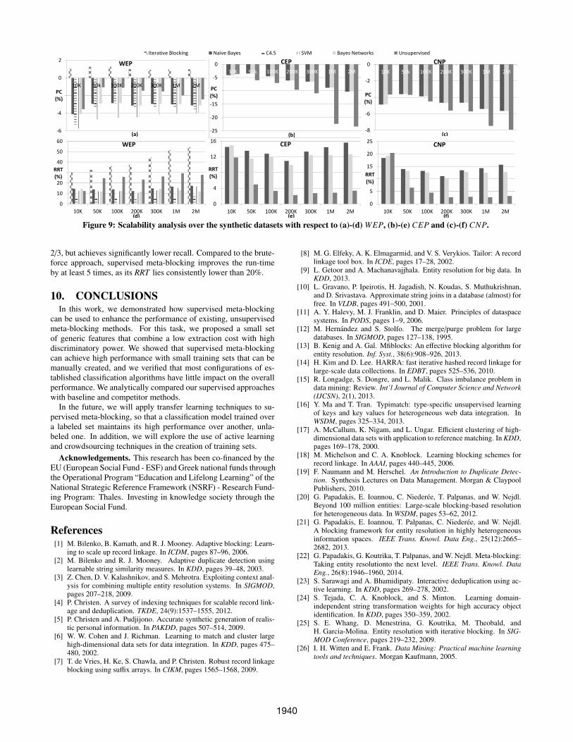
We applied supervised meta-blocking to WEP, CEP and CNP.The outcomes with respect to ∆PC are depicted in Figures 9(a)-(c),while RRT is presented in Figures 9(d)-(f).

WEP. We observe that iterative blocking consistently achievesthe highest effectiveness, increasing PC by 1%, at the cost of theworst efficiency across all datasets. In fact, its RRT increases mono-tonically for higher dataset sizes, raising from 1/3 to more than 1/2.On the other extreme lies supervised meta-blocking: it reduces PCby at least 3%, but requires at most 1/6 of the original resolutiontime. It scales well to larger datasets, as its performance is rela-tively stable across all datasets: for each classification algorithm,the difference between their maximum and minimum ∆PC is lessthan 2%, while for RRT it is less than 5%. In the middle of thesetwo extremes lies unsupervised meta-blocking, which reduces re-call by less than 3.5%, while requiring half of the resolution timeof iterative blocking. Note, though, that it does not scale well tolarger datasets, as its RRT raises from 1/6 for D10K to 1/3 for D2M .

CEP. For unsupervised meta-blocking, ∆PC decreases almostlinearly with the increase of the dataset size. In contrast, supervisedmeta-blocking scales well with respect to recall, as the variance ofits ∆PC is lower than 7% (note that both classification algorithmsexhibit practically identical performances). Equally stable is theirefficiency, since their RRT is close to 1/8, on average, while itsvariance is less than 5%. However, the run-time of unsupervisedmeta-blocking scales better, as its RRT decreases from 1/8 for D10K

to 1/30 for D2M .CNP. The efficiency of unsupervised meta-blocking scales well

with the increase of dataset size, dropping from 1/5 for D10K to 1/30for D2M , while its effectiveness decreases. In this case, though, itsrecall is close to that of supervised meta-blocking, with their max-imum difference amounting to 3%. In terms of efficiency, super-vised meta-blocking exhibits an unstable behavior, with its RRTfluctuating between 1/5 and 1/10.

Conclusions. Overall, we conclude that supervised meta-blockingscales better than the unsupervised one for WEP with respect toboth effectiveness and efficiency. For CEP, it scales better with re-spect to effectiveness, while unsupervised meta-blocking excels inefficiency in case a cheap entity matching method is employed. Thesame applies to CNP, as well. For this pruning algorithm, though,supervised meta-blocking improves effectiveness only to a minorextent. Compared to iterative blocking, supervised meta-blockingexcels in efficiency, requiring a lower resolution time by at least

1939

‐6

‐4

‐2

0

2

10K 50k 100K 200K 300K 1M 2MPC  (%) 

WEP 

Iterative Blocking Naïve Bayes C4.5 SVM Bayes Networks Unsupervised

(a)

‐6

‐4

‐2

0

2

10K 50k 100K 200K 300K 1M 2MPC  (%) 

WEP 

(a)‐25

‐20

‐15

‐10

‐5

0

10K 50k 100K 200K 300K 1M 2M

PC  (%) 

CEP 

(b)‐8

‐6

‐4

‐2

0

10K 50k 100K 200K 300K 1M 2M

PC  (%) 

CNP 

(c)

0

10

20

30

40

50

60

10K 50K 100K 200K 300K 1M 2M

RRT  (%) 

WEP 

(d)

0

4

8

12

16

10K 50K 100K 200K 300K 1M 2M

RRT  (%) 

CEP 

(e)

0

5

10

15

20

25

10K 50K 100K 200K 300K 1M 2M

RRT  (%) 

CNP 

(f)

Figure 9: Scalability analysis over the synthetic datasets with respect to (a)-(d) WEP, (b)-(e) CEP and (c)-(f) CNP.

2/3, but achieves significantly lower recall. Compared to the brute-force approach, supervised meta-blocking improves the run-timeby at least 5 times, as its RRT lies consistently lower than 20%.

10. CONCLUSIONSIn this work, we demonstrated how supervised meta-blocking

can be used to enhance the performance of existing, unsupervisedmeta-blocking methods. For this task, we proposed a small setof generic features that combine a low extraction cost with highdiscriminatory power. We showed that supervised meta-blockingcan achieve high performance with small training sets that can bemanually created, and we verified that most configurations of es-tablished classification algorithms have little impact on the overallperformance. We analytically compared our supervised approacheswith baseline and competitor methods.

In the future, we will apply transfer learning techniques to su-pervised meta-blocking, so that a classification model trained overa labeled set maintains its high performance over another, unla-beled one. In addition, we will explore the use of active learningand crowdsourcing techniques in the creation of training sets.

Acknowledgements. This research has been co-financed by theEU (European Social Fund - ESF) and Greek national funds throughthe Operational Program “Education and Lifelong Learning” of theNational Strategic Reference Framework (NSRF) - Research Fund-ing Program: Thales. Investing in knowledge society through theEuropean Social Fund.

References[1] M. Bilenko, B. Kamath, and R. J. Mooney. Adaptive blocking: Learn-

ing to scale up record linkage. In ICDM, pages 87–96, 2006.[2] M. Bilenko and R. J. Mooney. Adaptive duplicate detection using

learnable string similarity measures. In KDD, pages 39–48, 2003.[3] Z. Chen, D. V. Kalashnikov, and S. Mehrotra. Exploiting context anal-

ysis for combining multiple entity resolution systems. In SIGMOD,pages 207–218, 2009.

[4] P. Christen. A survey of indexing techniques for scalable record link-age and deduplication. TKDE, 24(9):1537–1555, 2012.

[5] P. Christen and A. Pudjijono. Accurate synthetic generation of realis-tic personal information. In PAKDD, pages 507–514, 2009.

[6] W. W. Cohen and J. Richman. Learning to match and cluster largehigh-dimensional data sets for data integration. In KDD, pages 475–480, 2002.

[7] T. de Vries, H. Ke, S. Chawla, and P. Christen. Robust record linkageblocking using suffix arrays. In CIKM, pages 1565–1568, 2009.

[8] M. G. Elfeky, A. K. Elmagarmid, and V. S. Verykios. Tailor: A recordlinkage tool box. In ICDE, pages 17–28, 2002.

[9] L. Getoor and A. Machanavajjhala. Entity resolution for big data. InKDD, 2013.

[10] L. Gravano, P. Ipeirotis, H. Jagadish, N. Koudas, S. Muthukrishnan,and D. Srivastava. Approximate string joins in a database (almost) forfree. In VLDB, pages 491–500, 2001.

[11] A. Y. Halevy, M. J. Franklin, and D. Maier. Principles of dataspacesystems. In PODS, pages 1–9, 2006.

[12] M. Hernandez and S. Stolfo. The merge/purge problem for largedatabases. In SIGMOD, pages 127–138, 1995.

[13] B. Kenig and A. Gal. Mfiblocks: An effective blocking algorithm forentity resolution. Inf. Syst., 38(6):908–926, 2013.

[14] H. Kim and D. Lee. HARRA: fast iterative hashed record linkage forlarge-scale data collections. In EDBT, pages 525–536, 2010.

[15] R. Longadge, S. Dongre, and L. Malik. Class imbalance problem indata mining: Review. Int’l Journal of Computer Science and Network(IJCSN), 2(1), 2013.

[16] Y. Ma and T. Tran. Typimatch: type-specific unsupervised learningof keys and key values for heterogeneous web data integration. InWSDM, pages 325–334, 2013.

[17] A. McCallum, K. Nigam, and L. Ungar. Efficient clustering of high-dimensional data sets with application to reference matching. In KDD,pages 169–178, 2000.

[18] M. Michelson and C. A. Knoblock. Learning blocking schemes forrecord linkage. In AAAI, pages 440–445, 2006.

[19] F. Naumann and M. Herschel. An Introduction to Duplicate Detec-tion. Synthesis Lectures on Data Management. Morgan & ClaypoolPublishers, 2010.

[20] G. Papadakis, E. Ioannou, C. Niederee, T. Palpanas, and W. Nejdl.Beyond 100 million entities: Large-scale blocking-based resolutionfor heterogeneous data. In WSDM, pages 53–62, 2012.

[21] G. Papadakis, E. Ioannou, T. Palpanas, C. Niederee, and W. Nejdl.A blocking framework for entity resolution in highly heterogeneousinformation spaces. IEEE Trans. Knowl. Data Eng., 25(12):2665–2682, 2013.

[22] G. Papadakis, G. Koutrika, T. Palpanas, and W. Nejdl. Meta-blocking:Taking entity resolutionto the next level. IEEE Trans. Knowl. DataEng., 26(8):1946–1960, 2014.

[23] S. Sarawagi and A. Bhamidipaty. Interactive deduplication using ac-tive learning. In KDD, pages 269–278, 2002.

[24] S. Tejada, C. A. Knoblock, and S. Minton. Learning domain-independent string transformation weights for high accuracy objectidentification. In KDD, pages 350–359, 2002.

[25] S. E. Whang, D. Menestrina, G. Koutrika, M. Theobald, andH. Garcia-Molina. Entity resolution with iterative blocking. In SIG-MOD Conference, pages 219–232, 2009.

[26] I. H. Witten and E. Frank. Data Mining: Practical machine learningtools and techniques. Morgan Kaufmann, 2005.

1940