Embed Size (px)
Citation preview

Supervised Learning(Part III)Weinan Zhang
Shanghai Jiao Tong Universityhttp://wnzhang.net
2019 EE448, Big Data Mining, Lecture 6
http://wnzhang.net/teaching/ee448/index.html
Content of Supervised Learning• Introduction to Machine Learning
• Linear Models
• Support Vector Machines
• Neural Networks
• Tree Models
• Ensemble Methods

Content of This Lecture
• Tree Models
• Ensemble Methods
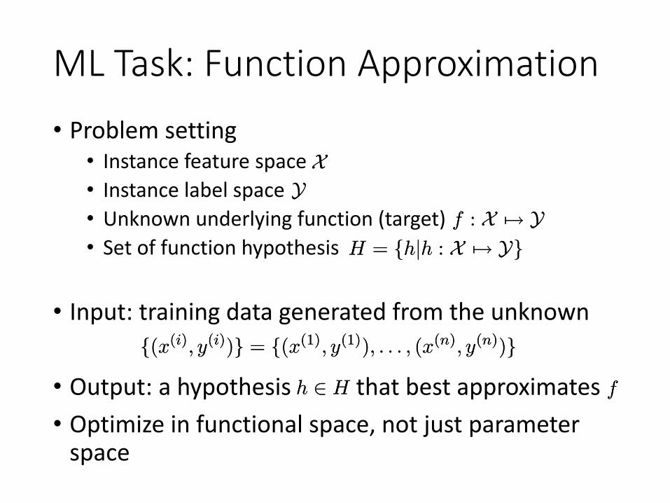
ML Task: Function Approximation• Problem setting
• Instance feature space• Instance label space• Unknown underlying function (target)• Set of function hypothesis
• Input: training data generated from the unknown
• Output: a hypothesis that best approximates• Optimize in functional space, not just parameter
space
XXYY
f : X 7! Yf : X 7! YH = fhjh : X 7! YgH = fhjh : X 7! Yg
f(x(i); y(i))g = f(x(1); y(1)); : : : ; (x(n); y(n))gf(x(i); y(i))g = f(x(1); y(1)); : : : ; (x(n); y(n))gh 2 Hh 2 H ff
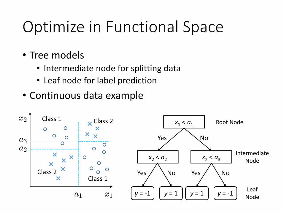
Optimize in Functional Space• Tree models
• Intermediate node for splitting data• Leaf node for label prediction
• Continuous data example
x1 < a1
x2 < a2 x2 < a3
Yes No
Yes No Yes No
IntermediateNode
LeafNode
Root Node
y = -1 y = 1 y = 1 y = -1x1x1
x2x2
a1a1
a2a2
Class 1
Class 2
a3a3
Class 1
Class 2
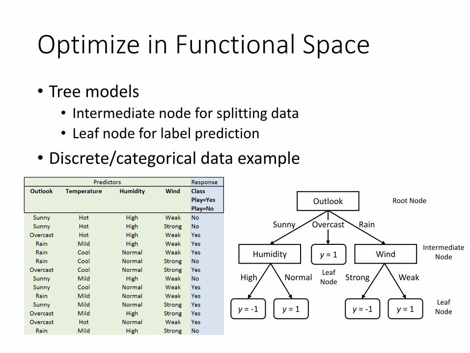
Optimize in Functional Space• Tree models
• Intermediate node for splitting data• Leaf node for label prediction
• Discrete/categorical data example
Outlook
Humidity Wind
Sunny Rain
High Normal Strong Weak
IntermediateNode
LeafNode
Root Node
y = -1 y = 1 y = -1 y = 1
y = 1
Overcast
LeafNode
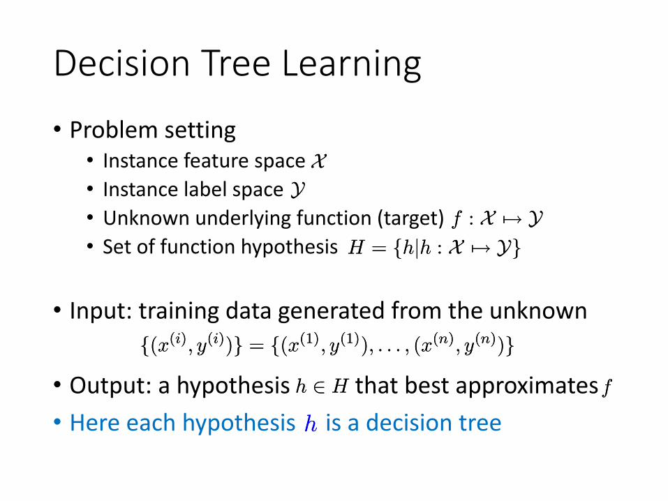
Decision Tree Learning• Problem setting
• Instance feature space• Instance label space• Unknown underlying function (target)• Set of function hypothesis
• Input: training data generated from the unknown
• Output: a hypothesis that best approximates• Here each hypothesis is a decision tree
XXYY
f : X 7! Yf : X 7! YH = fhjh : X 7! YgH = fhjh : X 7! Yg
f(x(i); y(i))g = f(x(1); y(1)); : : : ; (x(n); y(n))gf(x(i); y(i))g = f(x(1); y(1)); : : : ; (x(n); y(n))gh 2 Hh 2 H ff
hh
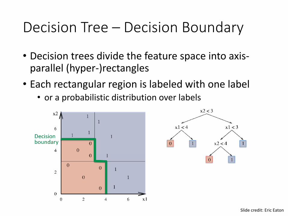
Decision Tree – Decision Boundary
• Decision trees divide the feature space into axis-parallel (hyper-)rectangles
• Each rectangular region is labeled with one label• or a probabilistic distribution over labels
Slide credit: Eric Eaton
History of Decision-Tree Research• Hunt and colleagues used exhaustive search decision-tree
methods (CLS) to model human concept learning in the 1960’s.
• In the late 70’s, Quinlan developed ID3 with the information gain heuristic to learn expert systems from examples.
• Simultaneously, Breiman and Friedman and colleagues developed CART (Classification and Regression Trees), similar to ID3.
• In the 1980’s a variety of improvements were introduced to handle noise, continuous features, missing features, and improved splitting criteria. Various expert-system development tools results.
• Quinlan’s updated decision-tree package (C4.5) released in 1993.
• Sklearn (python)Weka (Java) now include ID3 and C4.5
Slide credit: Raymond J. Mooney
Decision Trees• Tree models
• Intermediate node for splitting data• Leaf node for label prediction
• Key questions for decision trees• How to select node splitting conditions?• How to make prediction?• How to decide the tree structure?
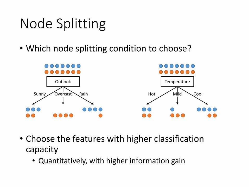
Node Splitting• Which node splitting condition to choose?
• Choose the features with higher classification capacity
• Quantitatively, with higher information gain
Outlook
Sunny RainOvercast
Temperature
Hot CoolMild
Fundamentals of Information Theory
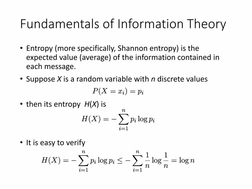
• Entropy (more specifically, Shannon entropy) is the expected value (average) of the information contained in each message.
• Suppose X is a random variable with n discrete values
• then its entropy H(X) is
H(X) = ¡nX
i=1
pi log piH(X) = ¡nX
i=1
pi log pi
P (X = xi) = piP (X = xi) = pi
• It is easy to verify
H(X) = ¡nX
i=1
pi log pi · ¡nX
i=1
1
nlog
1
n= log nH(X) = ¡
nXi=1
pi log pi · ¡nX
i=1
1
nlog
1
n= log n
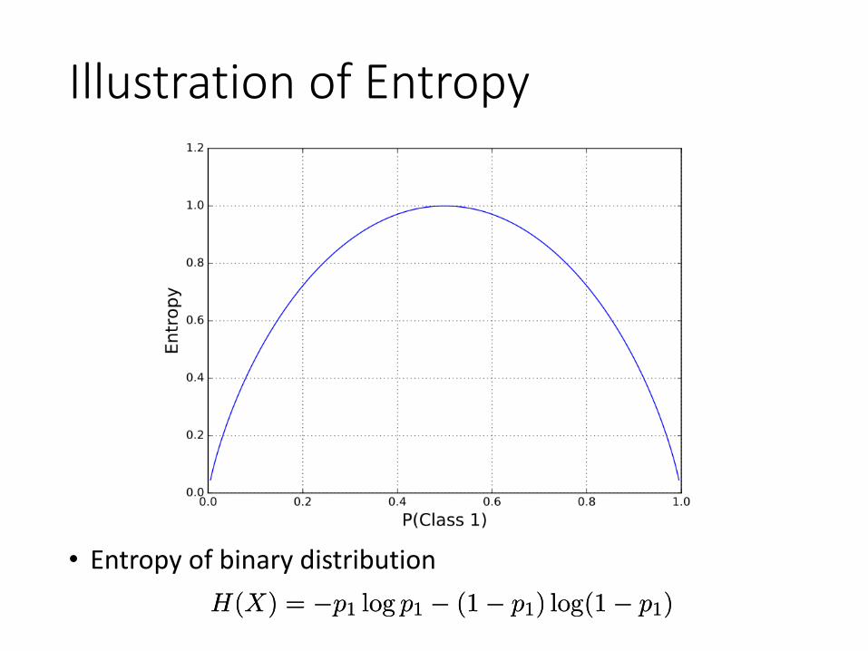
Illustration of Entropy
• Entropy of binary distributionH(X) = ¡p1 log p1 ¡ (1¡ p1) log(1¡ p1)H(X) = ¡p1 log p1 ¡ (1¡ p1) log(1¡ p1)
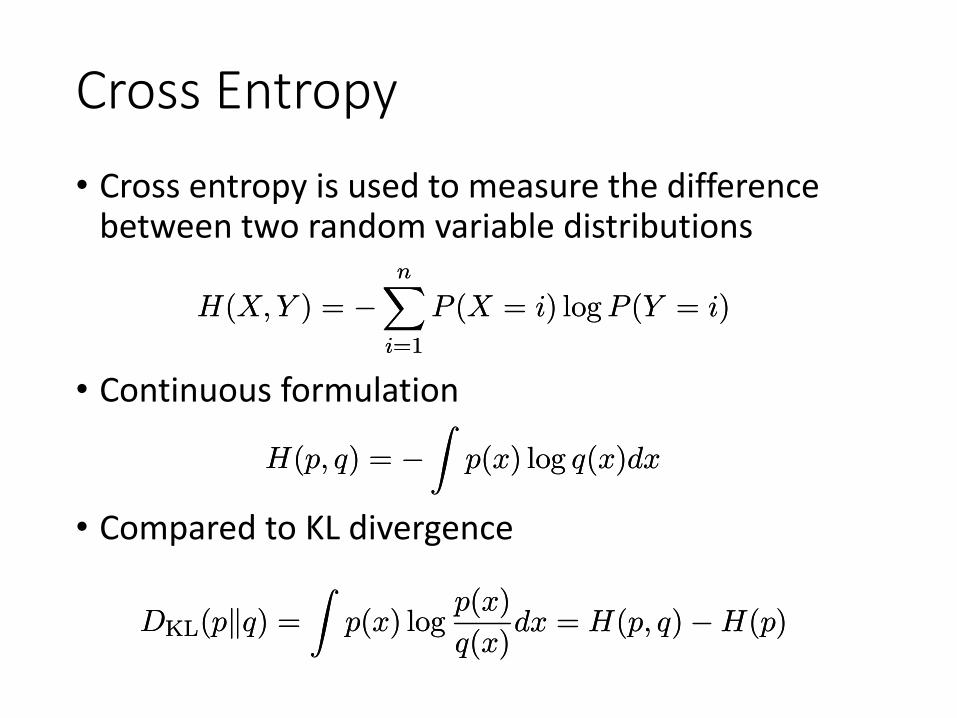
Cross Entropy• Cross entropy is used to measure the difference
between two random variable distributions
H(X; Y ) = ¡nX
i=1
P (X = i) log P (Y = i)H(X; Y ) = ¡nX
i=1
P (X = i) log P (Y = i)
• Continuous formulation
H(p; q) = ¡Z
p(x) log q(x)dxH(p; q) = ¡Z
p(x) log q(x)dx
• Compared to KL divergence
DKL(pkq) =
Zp(x) log
p(x)
q(x)dx = H(p; q)¡H(p)DKL(pkq) =
Zp(x) log
p(x)
q(x)dx = H(p; q)¡H(p)
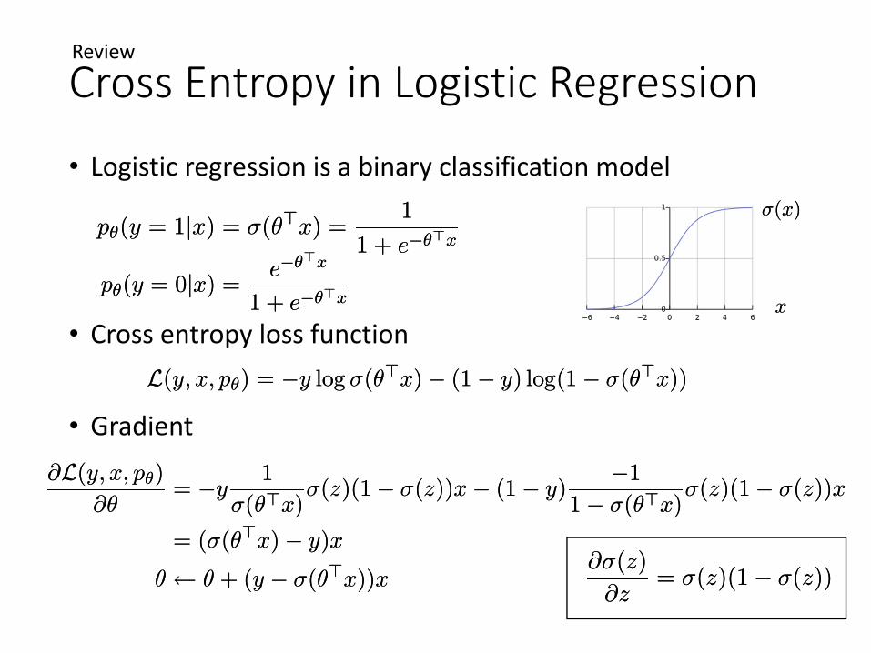
Cross Entropy in Logistic Regression
• Logistic regression is a binary classification model
pμ(y = 1jx) = ¾(μ>x) =1
1 + e¡μ>xpμ(y = 1jx) = ¾(μ>x) =
1
1 + e¡μ>x
pμ(y = 0jx) =e¡μ>x
1 + e¡μ>xpμ(y = 0jx) =
e¡μ>x
1 + e¡μ>x
L(y; x; pμ) = ¡y log ¾(μ>x)¡ (1 ¡ y) log(1¡ ¾(μ>x))L(y; x; pμ) = ¡y log ¾(μ>x)¡ (1 ¡ y) log(1¡ ¾(μ>x))
@¾(z)
@z= ¾(z)(1¡ ¾(z))
@¾(z)
@z= ¾(z)(1¡ ¾(z))
@L(y; x; pμ)
@μ= ¡y
1
¾(μ>x)¾(z)(1¡ ¾(z))x¡ (1¡ y)
¡1
1¡ ¾(μ>x)¾(z)(1¡ ¾(z))x
= (¾(μ>x)¡ y)x
μ Ã μ + (y ¡ ¾(μ>x))x
@L(y; x; pμ)
@μ= ¡y
1
¾(μ>x)¾(z)(1¡ ¾(z))x¡ (1¡ y)
¡1
1¡ ¾(μ>x)¾(z)(1¡ ¾(z))x
= (¾(μ>x)¡ y)x
μ Ã μ + (y ¡ ¾(μ>x))x
• Cross entropy loss function
• Gradient
¾(x)¾(x)
xx
Review
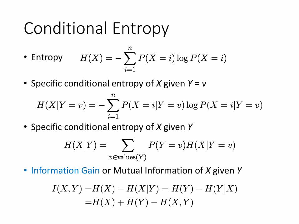
Conditional Entropy• Entropy H(X) = ¡
nXi=1
P (X = i) log P (X = i)H(X) = ¡nX
i=1
P (X = i) log P (X = i)
• Specific conditional entropy of X given Y = v
H(XjY = v) = ¡nX
i=1
P (X = ijY = v) log P (X = ijY = v)H(XjY = v) = ¡nX
i=1
P (X = ijY = v) log P (X = ijY = v)
• Specific conditional entropy of X given Y
H(XjY ) =X
v2values(Y )
P (Y = v)H(XjY = v)H(XjY ) =X
v2values(Y )
P (Y = v)H(XjY = v)
• Information Gain or Mutual Information of X given Y
I(X;Y ) =H(X)¡H(XjY ) = H(Y )¡H(Y jX)
=H(X) + H(Y )¡H(X;Y )
I(X;Y ) =H(X)¡H(XjY ) = H(Y )¡H(Y jX)
=H(X) + H(Y )¡H(X;Y )
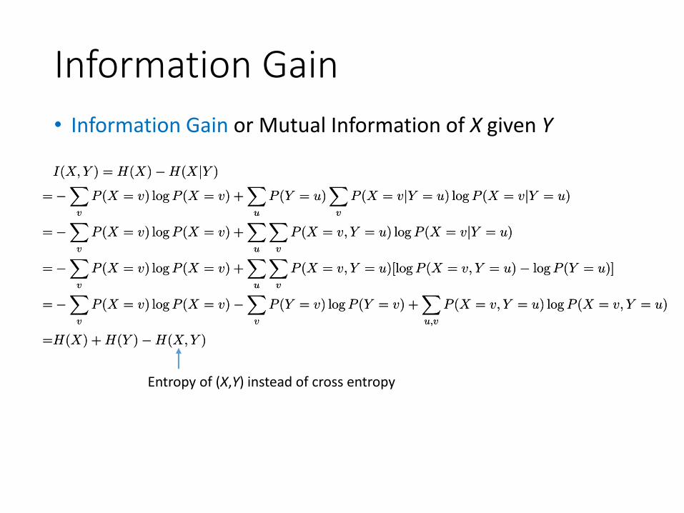
Information Gain• Information Gain or Mutual Information of X given Y
I(X;Y ) = H(X)¡H(XjY )
=¡X
v
P (X = v) log P (X = v) +X
u
P (Y = u)X
v
P (X = vjY = u) log P (X = vjY = u)
=¡X
v
P (X = v) log P (X = v) +X
u
Xv
P (X = v; Y = u) log P (X = vjY = u)
=¡X
v
P (X = v) log P (X = v) +X
u
Xv
P (X = v; Y = u)[log P (X = v; Y = u)¡ log P (Y = u)]
=¡X
v
P (X = v) log P (X = v)¡X
v
P (Y = v) log P (Y = v) +Xu;v
P (X = v; Y = u) log P (X = v; Y = u)
=H(X) + H(Y )¡H(X;Y )
Entropy of (X,Y) instead of cross entropy
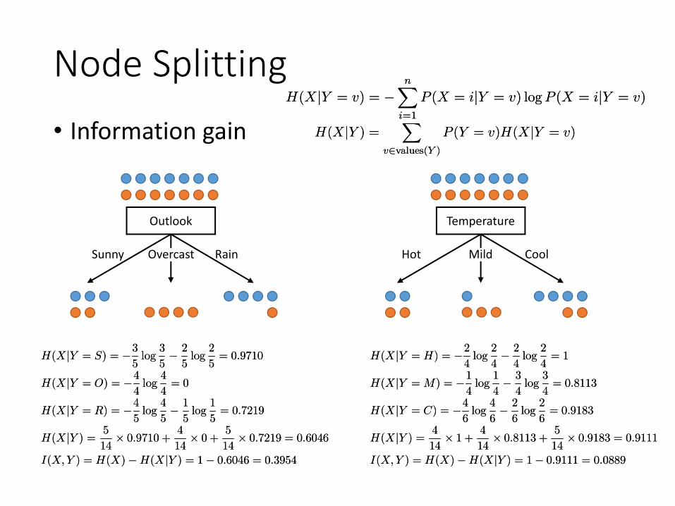
Node Splitting• Information gain
Outlook
Sunny RainOvercast
Temperature
Hot CoolMild
H(XjY = v) = ¡nX
i=1
P (X = ijY = v) log P (X = ijY = v)H(XjY = v) = ¡nX
i=1
P (X = ijY = v) log P (X = ijY = v)
H(XjY = S) = ¡3
5log
3
5¡ 2
5log
2
5= 0:9710
H(XjY = O) = ¡4
4log
4
4= 0
H(XjY = R) = ¡4
5log
4
5¡ 1
5log
1
5= 0:7219
H(XjY ) =5
14£ 0:9710 +
4
14£ 0 +
5
14£ 0:7219 = 0:6046
I(X;Y ) = H(X)¡H(XjY ) = 1¡ 0:6046 = 0:3954
H(XjY = S) = ¡3
5log
3
5¡ 2
5log
2
5= 0:9710
H(XjY = O) = ¡4
4log
4
4= 0
H(XjY = R) = ¡4
5log
4
5¡ 1
5log
1
5= 0:7219
H(XjY ) =5
14£ 0:9710 +
4
14£ 0 +
5
14£ 0:7219 = 0:6046
I(X;Y ) = H(X)¡H(XjY ) = 1¡ 0:6046 = 0:3954
H(XjY ) =X
v2values(Y )
P (Y = v)H(XjY = v)H(XjY ) =X
v2values(Y )
P (Y = v)H(XjY = v)
H(XjY = H) = ¡2
4log
2
4¡ 2
4log
2
4= 1
H(XjY = M) = ¡1
4log
1
4¡ 3
4log
3
4= 0:8113
H(XjY = C) = ¡4
6log
4
6¡ 2
6log
2
6= 0:9183
H(XjY ) =4
14£ 1 +
4
14£ 0:8113 +
5
14£ 0:9183 = 0:9111
I(X;Y ) = H(X)¡H(XjY ) = 1¡ 0:9111 = 0:0889
H(XjY = H) = ¡2
4log
2
4¡ 2
4log
2
4= 1
H(XjY = M) = ¡1
4log
1
4¡ 3
4log
3
4= 0:8113
H(XjY = C) = ¡4
6log
4
6¡ 2
6log
2
6= 0:9183
H(XjY ) =4
14£ 1 +
4
14£ 0:8113 +
5
14£ 0:9183 = 0:9111
I(X;Y ) = H(X)¡H(XjY ) = 1¡ 0:9111 = 0:0889
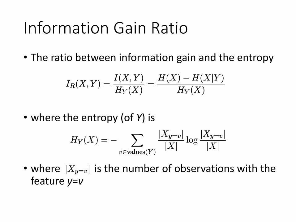
Information Gain Ratio• The ratio between information gain and the entropy
IR(X;Y ) =I(X;Y )
HY (X)=
H(X)¡H(XjY )
HY (X)IR(X;Y ) =
I(X;Y )
HY (X)=
H(X)¡H(XjY )
HY (X)
HY (X) = ¡X
v2values(Y )
jXy=vjjXj log
jXy=vjjXjHY (X) = ¡
Xv2values(Y )
jXy=vjjXj log
jXy=vjjXj
• where the entropy (of Y) is
• where is the number of observations with the feature y=v
jXy=vjjXy=vj
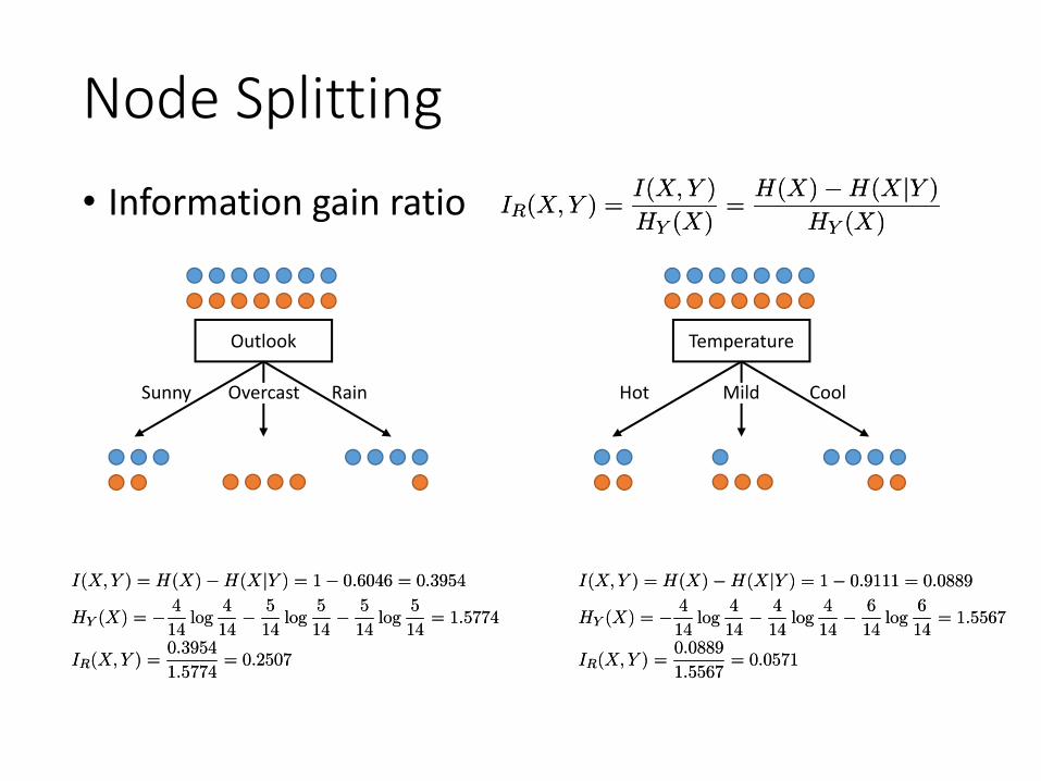
Node Splitting• Information gain ratio
Outlook
Sunny RainOvercast
Temperature
Hot CoolMild
I(X;Y ) = H(X)¡H(XjY ) = 1¡ 0:6046 = 0:3954
HY (X) = ¡ 4
14log
4
14¡ 5
14log
5
14¡ 5
14log
5
14= 1:5774
IR(X;Y ) =0:3954
1:5774= 0:2507
I(X;Y ) = H(X)¡H(XjY ) = 1¡ 0:6046 = 0:3954
HY (X) = ¡ 4
14log
4
14¡ 5
14log
5
14¡ 5
14log
5
14= 1:5774
IR(X;Y ) =0:3954
1:5774= 0:2507
I(X;Y ) = H(X)¡H(XjY ) = 1¡ 0:9111 = 0:0889
HY (X) = ¡ 4
14log
4
14¡ 4
14log
4
14¡ 6
14log
6
14= 1:5567
IR(X;Y ) =0:0889
1:5567= 0:0571
I(X;Y ) = H(X)¡H(XjY ) = 1¡ 0:9111 = 0:0889
HY (X) = ¡ 4
14log
4
14¡ 4
14log
4
14¡ 6
14log
6
14= 1:5567
IR(X;Y ) =0:0889
1:5567= 0:0571
IR(X;Y ) =I(X;Y )
HY (X)=
H(X)¡H(XjY )
HY (X)IR(X;Y ) =
I(X;Y )
HY (X)=
H(X)¡H(XjY )
HY (X)
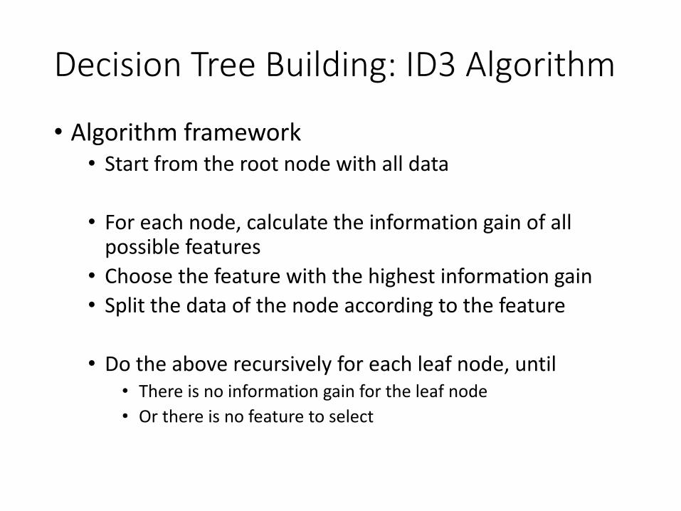
Decision Tree Building: ID3 Algorithm
• Algorithm framework• Start from the root node with all data
• For each node, calculate the information gain of all possible features
• Choose the feature with the highest information gain• Split the data of the node according to the feature
• Do the above recursively for each leaf node, until • There is no information gain for the leaf node• Or there is no feature to select
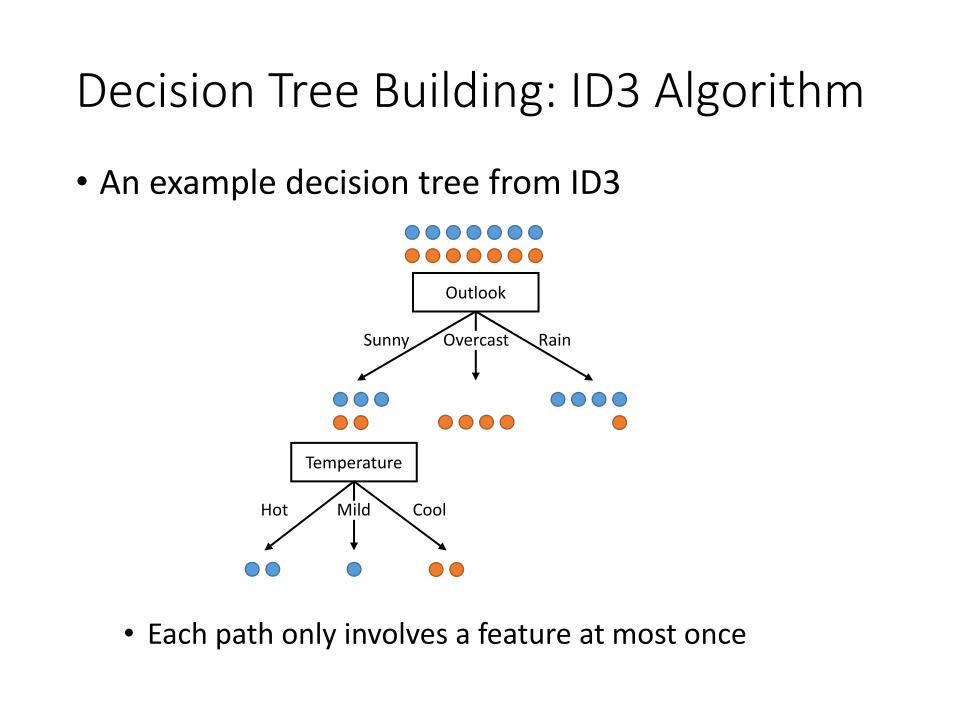
Decision Tree Building: ID3 Algorithm
• An example decision tree from ID3
Outlook
Sunny RainOvercast
Temperature
Hot CoolMild
• Each path only involves a feature at most once
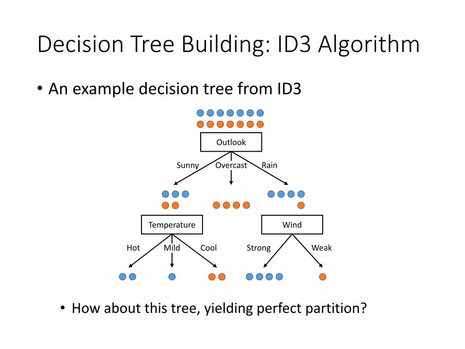
Decision Tree Building: ID3 Algorithm
• An example decision tree from ID3
Outlook
Sunny RainOvercast
Temperature
Hot CoolMild
Wind
Strong Weak
• How about this tree, yielding perfect partition?
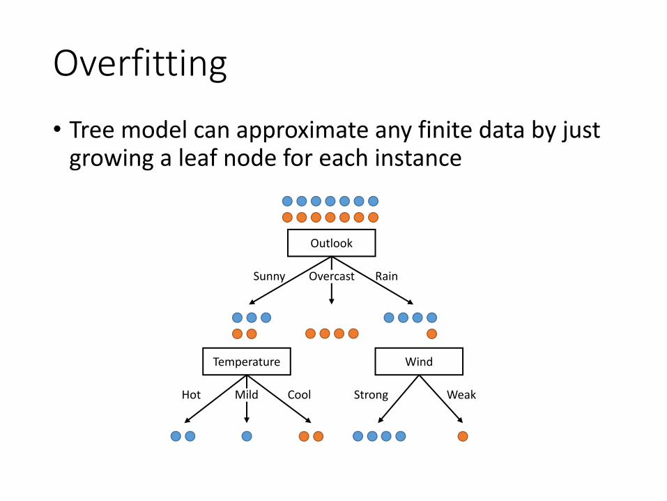
Overfitting• Tree model can approximate any finite data by just
growing a leaf node for each instance
Outlook
Sunny RainOvercast
Temperature
Hot CoolMild
Wind
Strong Weak
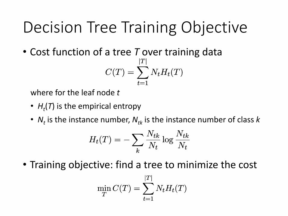
Decision Tree Training Objective• Cost function of a tree T over training data
C(T ) =
jT jXt=1
NtHt(T )C(T ) =
jT jXt=1
NtHt(T )
where for the leaf node t• Ht(T) is the empirical entropy• Nt is the instance number, Ntk is the instance number of class k
Ht(T ) = ¡X
k
Ntk
Ntlog
Ntk
NtHt(T ) = ¡
Xk
Ntk
Ntlog
Ntk
Nt
• Training objective: find a tree to minimize the cost
minT
C(T ) =
jT jXt=1
NtHt(T )minT
C(T ) =
jT jXt=1
NtHt(T )
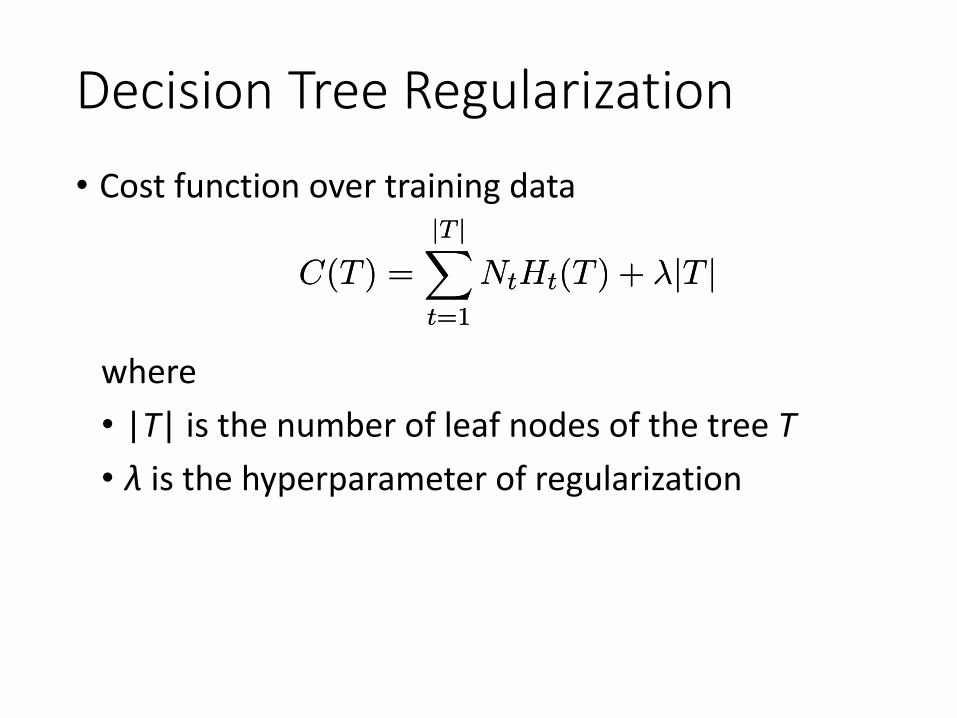
Decision Tree Regularization• Cost function over training data
C(T ) =
jT jXt=1
NtHt(T ) + ¸jT jC(T ) =
jT jXt=1
NtHt(T ) + ¸jT j
where • |T| is the number of leaf nodes of the tree T• λ is the hyperparameter of regularization
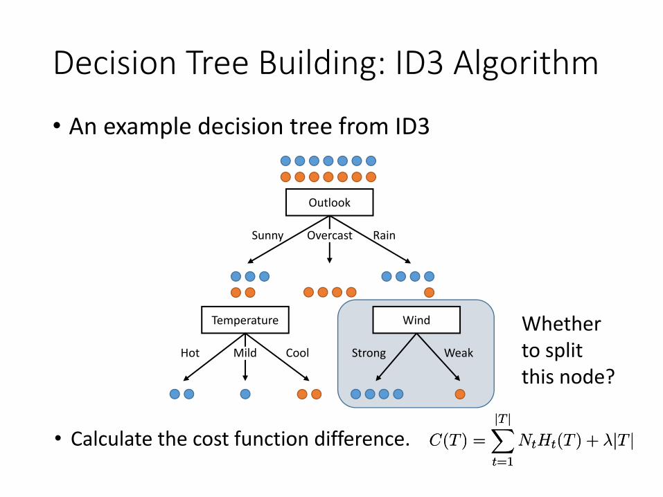
Decision Tree Building: ID3 Algorithm
• An example decision tree from ID3
Outlook
Sunny RainOvercast
Temperature
Hot CoolMild
Wind
Strong Weak
• Calculate the cost function difference. C(T ) =
jT jXt=1
NtHt(T ) + ¸jT jC(T ) =
jT jXt=1
NtHt(T ) + ¸jT j
Whether to split this node?
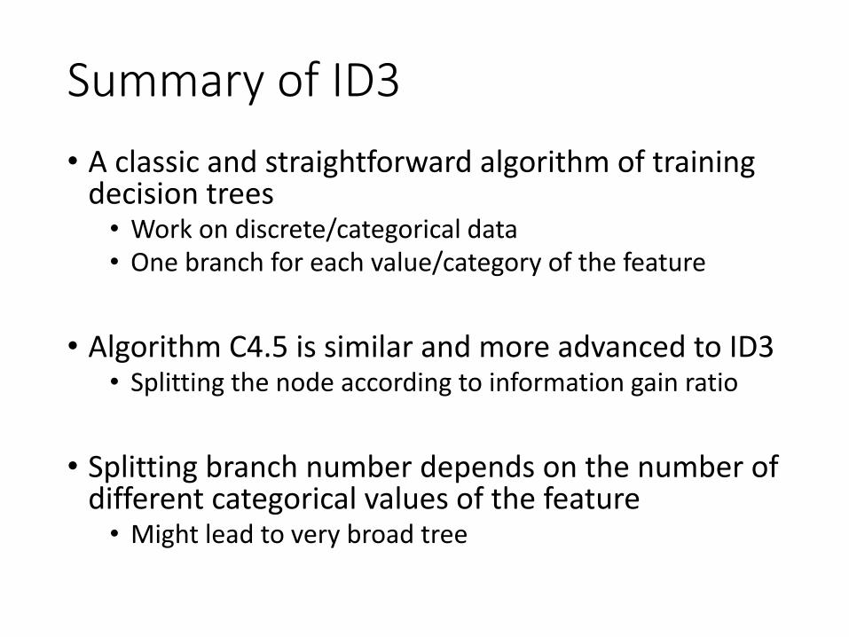
Summary of ID3• A classic and straightforward algorithm of training
decision trees• Work on discrete/categorical data• One branch for each value/category of the feature
• Algorithm C4.5 is similar and more advanced to ID3• Splitting the node according to information gain ratio
• Splitting branch number depends on the number of different categorical values of the feature
• Might lead to very broad tree
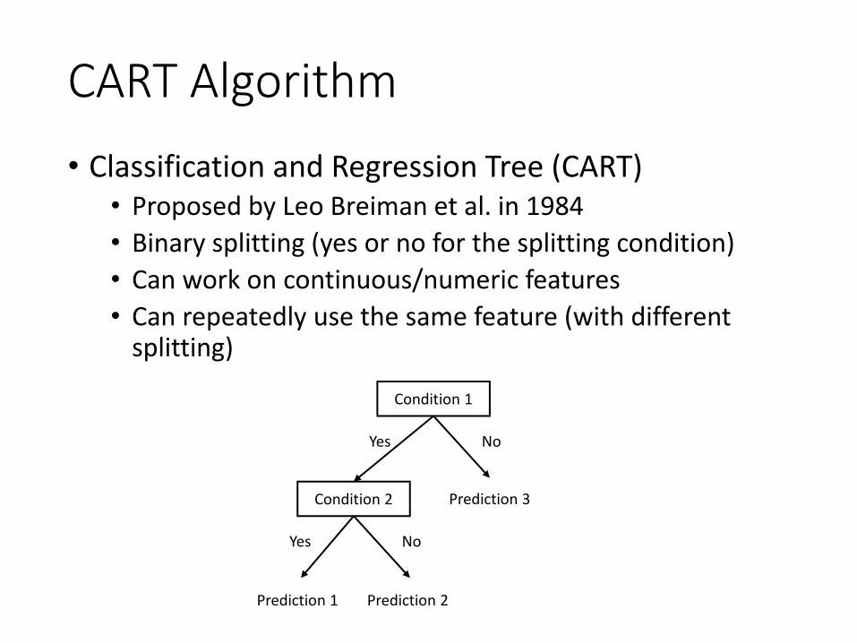
CART Algorithm• Classification and Regression Tree (CART)
• Proposed by Leo Breiman et al. in 1984• Binary splitting (yes or no for the splitting condition)• Can work on continuous/numeric features• Can repeatedly use the same feature (with different
splitting)
Condition 1
Yes No
Condition 2
Yes No
Prediction 1 Prediction 2
Prediction 3
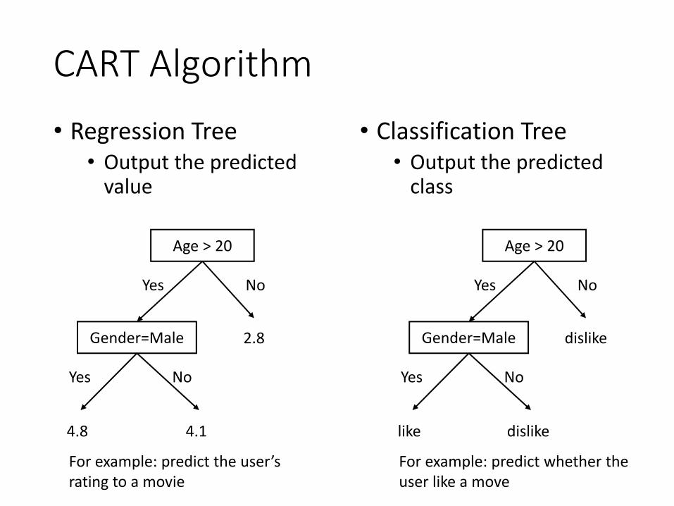
CART Algorithm• Classification Tree
• Output the predicted class
Age > 20
Yes No
Gender=Male
Yes No
4.8 4.1
2.8
• Regression Tree• Output the predicted
value
Age > 20
Yes No
Gender=Male
Yes No
like dislike
dislike
For example: predict the user’s rating to a movie
For example: predict whether the user like a move
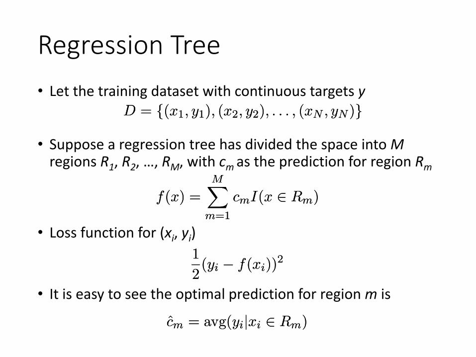
Regression Tree• Let the training dataset with continuous targets y
D = f(x1; y1); (x2; y2); : : : ; (xN ; yN )gD = f(x1; y1); (x2; y2); : : : ; (xN ; yN )g
• Suppose a regression tree has divided the space into Mregions R1, R2, …, RM, with cm as the prediction for region Rm
f(x) =MX
m=1
cmI(x 2 Rm)f(x) =MX
m=1
cmI(x 2 Rm)
• Loss function for (xi, yi)1
2(yi ¡ f(xi))
21
2(yi ¡ f(xi))
2
• It is easy to see the optimal prediction for region m is
cm = avg(yijxi 2 Rm)cm = avg(yijxi 2 Rm)
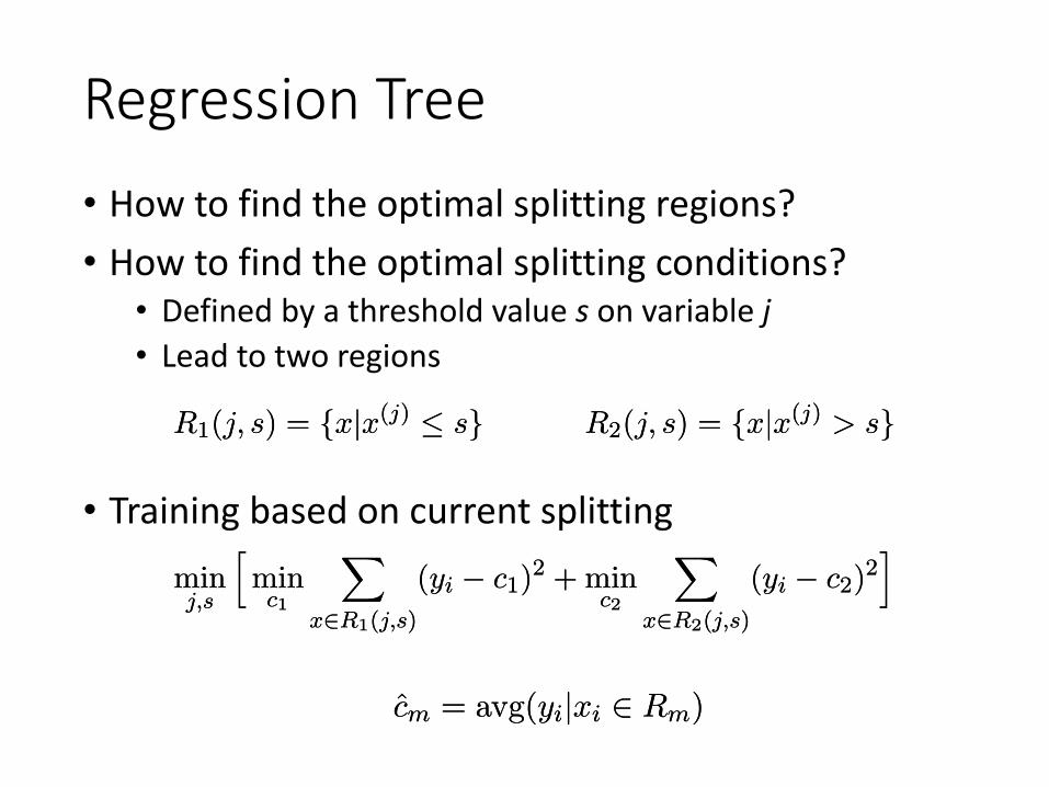
Regression Tree• How to find the optimal splitting regions?• How to find the optimal splitting conditions?
• Defined by a threshold value s on variable j• Lead to two regions
R1(j; s) = fxjx(j) · sgR1(j; s) = fxjx(j) · sg R2(j; s) = fxjx(j) > sgR2(j; s) = fxjx(j) > sg
minj;s
hminc1
Xx2R1(j;s)
(yi ¡ c1)2 + min
c2
Xx2R2(j;s)
(yi ¡ c2)2i
minj;s
hminc1
Xx2R1(j;s)
(yi ¡ c1)2 + min
c2
Xx2R2(j;s)
(yi ¡ c2)2i• Training based on current splitting
cm = avg(yijxi 2 Rm)cm = avg(yijxi 2 Rm)
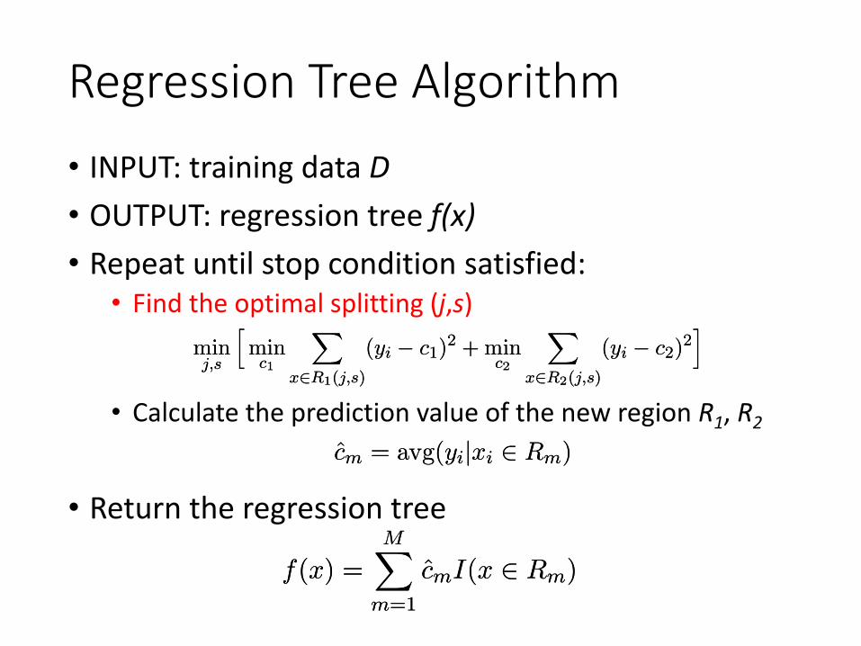
Regression Tree Algorithm• INPUT: training data D• OUTPUT: regression tree f(x)• Repeat until stop condition satisfied:
• Find the optimal splitting (j,s)minj;s
hminc1
Xx2R1(j;s)
(yi ¡ c1)2 + min
c2
Xx2R2(j;s)
(yi ¡ c2)2i
minj;s
hminc1
Xx2R1(j;s)
(yi ¡ c1)2 + min
c2
Xx2R2(j;s)
(yi ¡ c2)2i
• Calculate the prediction value of the new region R1, R2cm = avg(yijxi 2 Rm)cm = avg(yijxi 2 Rm)
• Return the regression tree
f(x) =MX
m=1
cmI(x 2 Rm)f(x) =MX
m=1
cmI(x 2 Rm)
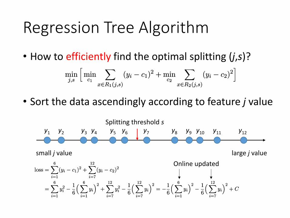
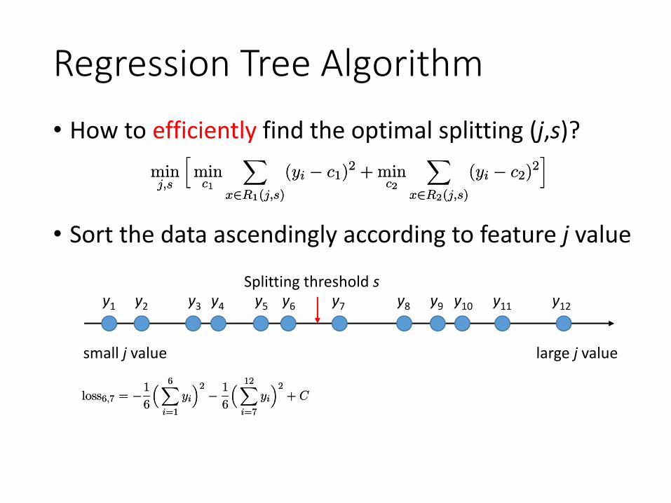
Regression Tree Algorithm• How to efficiently find the optimal splitting (j,s)?
minj;s
hminc1
Xx2R1(j;s)
(yi ¡ c1)2 + min
c2
Xx2R2(j;s)
(yi ¡ c2)2i
minj;s
hminc1
Xx2R1(j;s)
(yi ¡ c1)2 + min
c2
Xx2R2(j;s)
(yi ¡ c2)2i
• Sort the data ascendingly according to feature j value
small j value large j value
Splitting threshold sy1 y2 y3 y4 y5 y6 y7 y8 y9 y10 y11 y12
loss =
6Xi=1
(yi ¡ c1)2 +
12Xi=7
(yi ¡ c2)2
=
6Xi=1
y2i ¡
1
6
³ 6Xi=1
yi
´2+
12Xi=7
y2i ¡
1
6
³ 12Xi=7
yi
´2= ¡1
6
³ 6Xi=1
yi
´2 ¡ 1
6
³ 12Xi=7
yi
´2+ C
loss =
6Xi=1
(yi ¡ c1)2 +
12Xi=7
(yi ¡ c2)2
=
6Xi=1
y2i ¡
1
6
³ 6Xi=1
yi
´2+
12Xi=7
y2i ¡
1
6
³ 12Xi=7
yi
´2= ¡1
6
³ 6Xi=1
yi
´2 ¡ 1
6
³ 12Xi=7
yi
´2+ C
Online updated
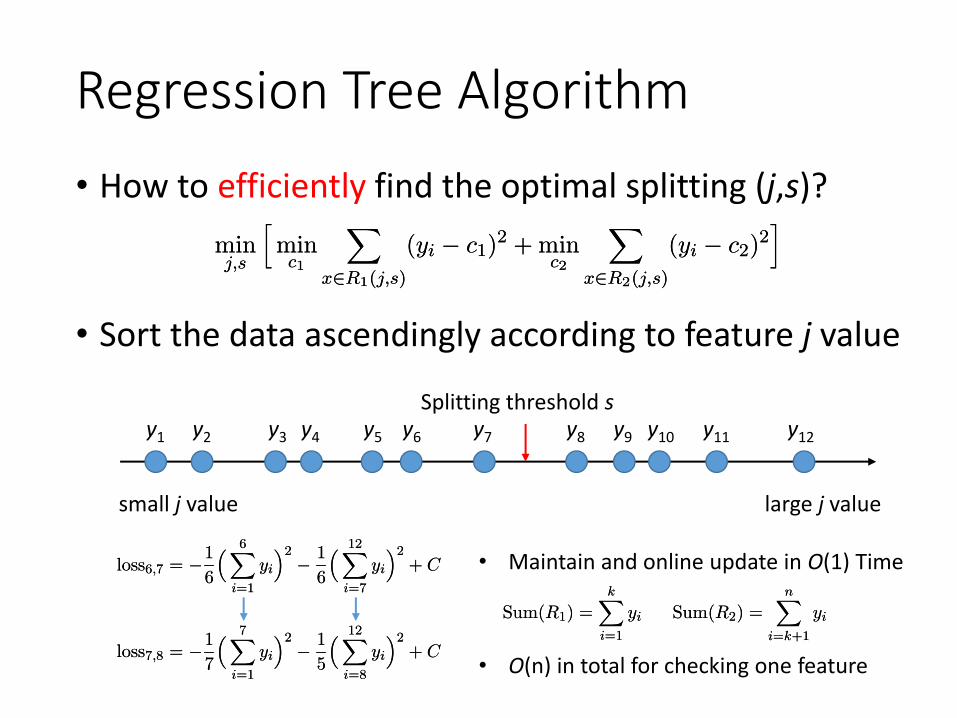
Regression Tree Algorithm• How to efficiently find the optimal splitting (j,s)?
minj;s
hminc1
Xx2R1(j;s)
(yi ¡ c1)2 + min
c2
Xx2R2(j;s)
(yi ¡ c2)2i
minj;s
hminc1
Xx2R1(j;s)
(yi ¡ c1)2 + min
c2
Xx2R2(j;s)
(yi ¡ c2)2i
• Sort the data ascendingly according to feature j value
small j value large j value
y1 y2 y3 y4 y5 y6 y7 y8 y9 y10 y11 y12
Splitting threshold s
loss6;7 = ¡1
6
³ 6Xi=1
yi
´2 ¡ 1
6
³ 12Xi=7
yi
´2+ Closs6;7 = ¡1
6
³ 6Xi=1
yi
´2 ¡ 1
6
³ 12Xi=7
yi
´2+ C
Regression Tree Algorithm• How to efficiently find the optimal splitting (j,s)?
minj;s
hminc1
Xx2R1(j;s)
(yi ¡ c1)2 + min
c2
Xx2R2(j;s)
(yi ¡ c2)2i
minj;s
hminc1
Xx2R1(j;s)
(yi ¡ c1)2 + min
c2
Xx2R2(j;s)
(yi ¡ c2)2i
• Sort the data ascendingly according to feature j value
small j value large j value
Splitting threshold sy1 y2 y3 y4 y5 y6 y7 y8 y9 y10 y11 y12
loss6;7 = ¡1
6
³ 6Xi=1
yi
´2 ¡ 1
6
³ 12Xi=7
yi
´2+ Closs6;7 = ¡1
6
³ 6Xi=1
yi
´2 ¡ 1
6
³ 12Xi=7
yi
´2+ C • Maintain and online update in O(1) Time
loss7;8 = ¡1
7
³ 7Xi=1
yi
´2 ¡ 1
5
³ 12Xi=8
yi
´2+ Closs7;8 = ¡1
7
³ 7Xi=1
yi
´2 ¡ 1
5
³ 12Xi=8
yi
´2+ C
Sum(R1) =kX
i=1
yi Sum(R2) =nX
i=k+1
yiSum(R1) =kX
i=1
yi Sum(R2) =nX
i=k+1
yi
• O(n) in total for checking one feature
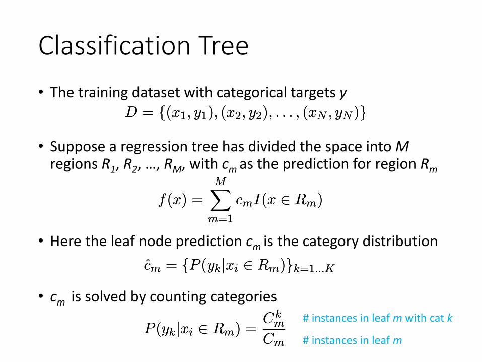
Classification Tree• The training dataset with categorical targets y
D = f(x1; y1); (x2; y2); : : : ; (xN ; yN )gD = f(x1; y1); (x2; y2); : : : ; (xN ; yN )g
• Suppose a regression tree has divided the space into Mregions R1, R2, …, RM, with cm as the prediction for region Rm
f(x) =MX
m=1
cmI(x 2 Rm)f(x) =MX
m=1
cmI(x 2 Rm)
• cm is solved by counting categories
P (ykjxi 2 Rm) =Ck
m
CmP (ykjxi 2 Rm) =
Ckm
Cm
• Here the leaf node prediction cm is the category distributioncm = fP (ykjxi 2 Rm)gk=1:::Kcm = fP (ykjxi 2 Rm)gk=1:::K
# instances in leaf m with cat k
# instances in leaf m
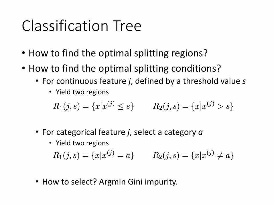
Classification Tree• How to find the optimal splitting regions?• How to find the optimal splitting conditions?
• For continuous feature j, defined by a threshold value s• Yield two regions
R1(j; s) = fxjx(j) · sgR1(j; s) = fxjx(j) · sg R2(j; s) = fxjx(j) > sgR2(j; s) = fxjx(j) > sg
• For categorical feature j, select a category a• Yield two regionsR1(j; s) = fxjx(j) = agR1(j; s) = fxjx(j) = ag R2(j; s) = fxjx(j) 6= agR2(j; s) = fxjx(j) 6= ag
• How to select? Argmin Gini impurity.
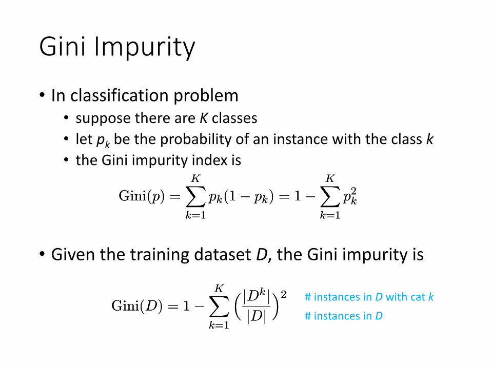
Gini Impurity• In classification problem
• suppose there are K classes• let pk be the probability of an instance with the class k• the Gini impurity index is
Gini(p) =
KXk=1
pk(1¡ pk) = 1¡KX
k=1
p2kGini(p) =
KXk=1
pk(1¡ pk) = 1¡KX
k=1
p2k
• Given the training dataset D, the Gini impurity is
Gini(D) = 1¡KX
k=1
³ jDkjjDj
´2Gini(D) = 1¡
KXk=1
³ jDkjjDj
´2 # instances in D with cat k# instances in D
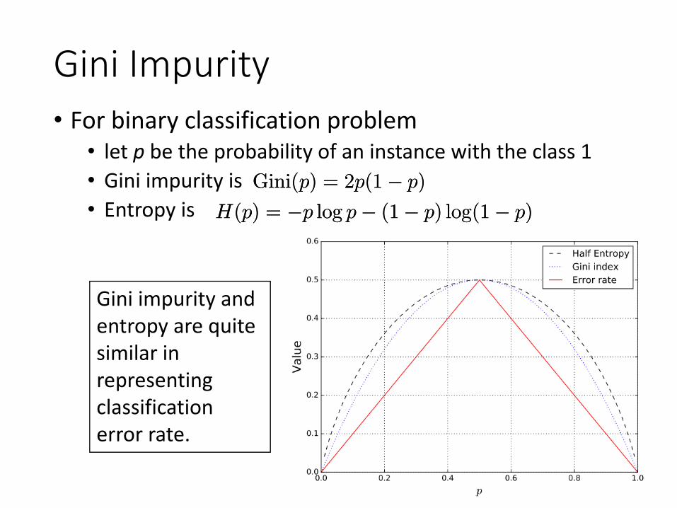
Gini Impurity• For binary classification problem
• let p be the probability of an instance with the class 1• Gini impurity is• Entropy is
Gini(p) = 2p(1¡ p)Gini(p) = 2p(1¡ p)
Gini impurity and entropy are quite similar in representing classification error rate.
H(p) = ¡p log p¡ (1¡ p) log(1¡ p)H(p) = ¡p log p¡ (1¡ p) log(1¡ p)
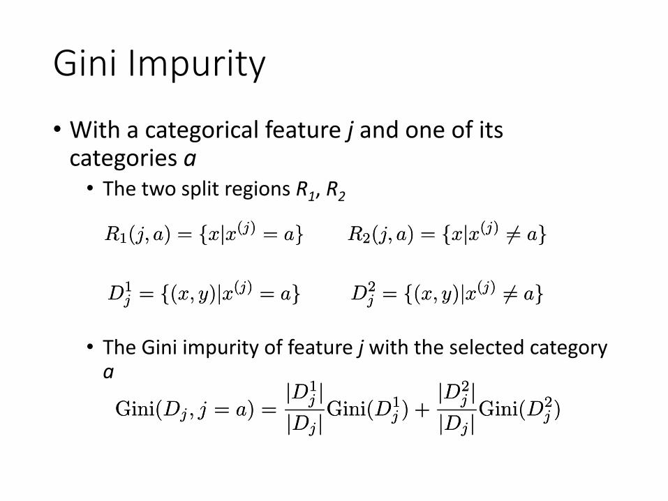
Gini Impurity• With a categorical feature j and one of its
categories a• The two split regions R1, R2
R1(j; a) = fxjx(j) = agR1(j; a) = fxjx(j) = ag R2(j; a) = fxjx(j) 6= agR2(j; a) = fxjx(j) 6= ag
• The Gini impurity of feature j with the selected category a
Gini(Dj ; j = a) =jD1
j jjDj jGini(D1
j ) +jD2
j jjDj jGini(D2
j )Gini(Dj ; j = a) =jD1
j jjDj jGini(D1
j ) +jD2
j jjDj jGini(D2
j )
D1j = f(x; y)jx(j) = agD1j = f(x; y)jx(j) = ag D2
j = f(x; y)jx(j) 6= agD2j = f(x; y)jx(j) 6= ag
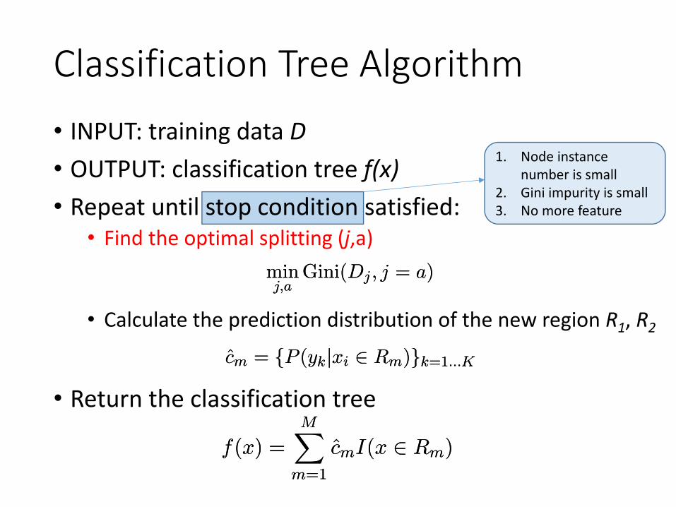
Classification Tree Algorithm• INPUT: training data D• OUTPUT: classification tree f(x)• Repeat until stop condition satisfied:
• Find the optimal splitting (j,a)minj;a
Gini(Dj ; j = a)minj;a
Gini(Dj ; j = a)
• Calculate the prediction distribution of the new region R1, R2
cm = fP (ykjxi 2 Rm)gk=1:::Kcm = fP (ykjxi 2 Rm)gk=1:::K
• Return the classification tree
f(x) =MX
m=1
cmI(x 2 Rm)f(x) =MX
m=1
cmI(x 2 Rm)
1. Node instance number is small
2. Gini impurity is small3. No more feature
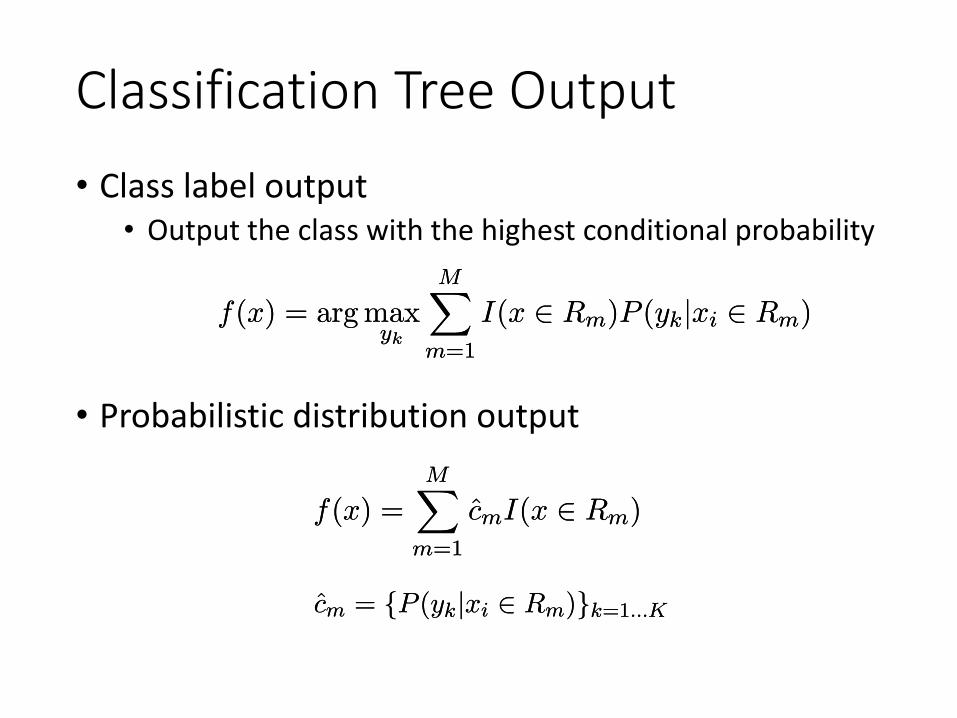
Classification Tree Output• Class label output
• Output the class with the highest conditional probability
f(x) =MX
m=1
cmI(x 2 Rm)f(x) =MX
m=1
cmI(x 2 Rm)
• Probabilistic distribution output
f(x) = arg maxyk
MXm=1
I(x 2 Rm)P (ykjxi 2 Rm)f(x) = arg maxyk
MXm=1
I(x 2 Rm)P (ykjxi 2 Rm)
cm = fP (ykjxi 2 Rm)gk=1:::Kcm = fP (ykjxi 2 Rm)gk=1:::K
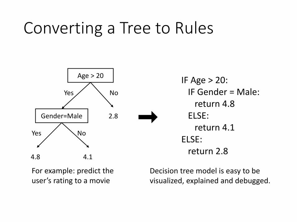
Converting a Tree to Rules
Age > 20
Yes No
Gender=Male
Yes No
4.8 4.1
2.8
For example: predict the user’s rating to a movie
IF Age > 20:IF Gender = Male:
return 4.8ELSE:
return 4.1ELSE:
return 2.8
Decision tree model is easy to be visualized, explained and debugged.
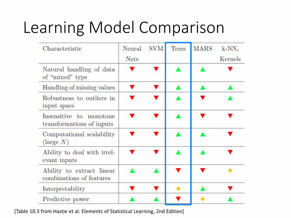
Learning Model Comparison
[Table 10.3 from Hastie et al. Elements of Statistical Learning, 2nd Edition]

Content of This Lecture
• Tree Models
• Ensemble Methods
Ensemble LearningBaggingRandom Forest
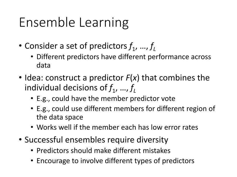
Ensemble Learning• Consider a set of predictors f1, …, fL
• Different predictors have different performance across data
• Idea: construct a predictor F(x) that combines the individual decisions of f1, …, fL
• E.g., could have the member predictor vote• E.g., could use different members for different region of
the data space• Works well if the member each has low error rates
• Successful ensembles require diversity• Predictors should make different mistakes• Encourage to involve different types of predictors
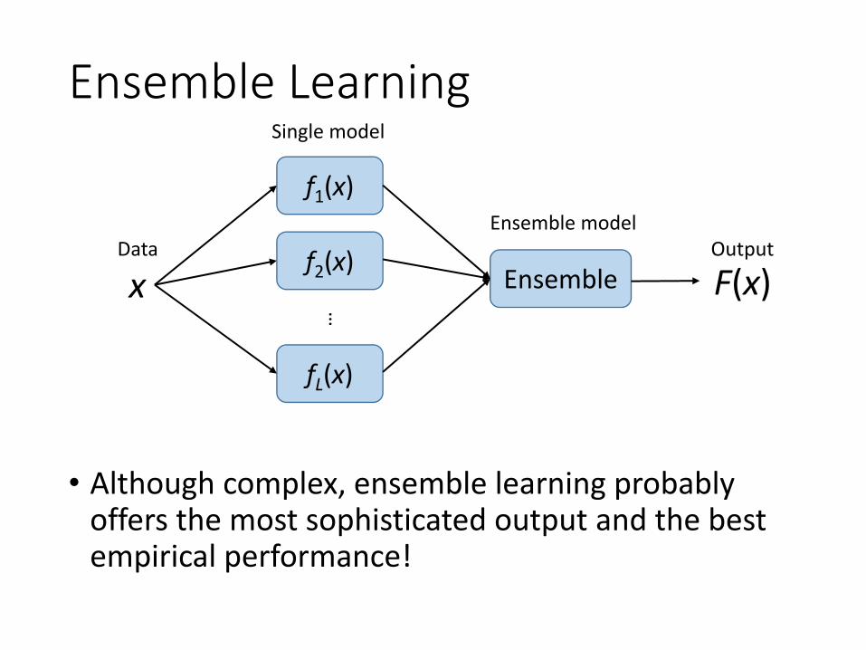
Ensemble Learning
• Although complex, ensemble learning probably offers the most sophisticated output and the best empirical performance!
x
f1(x)
f2(x)
fL(x)
…
Ensemble F(x)Data
Single model
Ensemble modelOutput

Practical Application in Competitions
• Netflix Prize Competition• Task: predict the user’s rating on a movie, given some
users’ ratings on some movies• Called ‘collaborative filtering’ (we will have a lecture
about it later)
[Yehuda Koren. The BellKor Solution to the Netflix Grand Prize. 2009.]
• Winner solution• BellKor’s Pragmatic Chaos – an
ensemble of more than 800 predictors
Yehuda Koren

Practical Application in Competitions• KDD-Cup 2011 Yahoo! Music Recommendation
• Task: predict the user’s rating on a music, given some users’ ratings on some music
• With music information like album, artist, genre IDs
• Winner solution• From A graduate course of National Taiwan University -
an ensemble of 221 predictors

Practical Application in Competitions• KDD-Cup 2011 Yahoo! Music Recommendation
• Task: predict the user’s rating on a music, given some users’ ratings on some music
• With music information like album, artist, genre IDs
• 3rd place solution• SJTU-HKUST joint team, an ensemble of 16 predictors
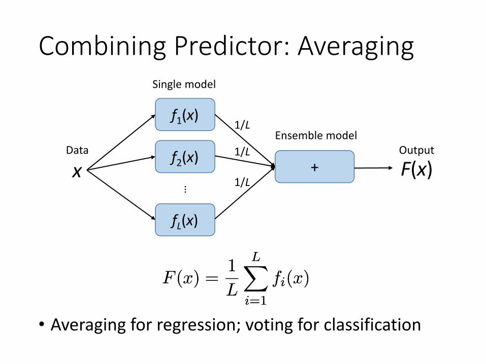
Combining Predictor: Averaging
• Averaging for regression; voting for classification
x
f1(x)
f2(x)
fL(x)
…
+ F(x)Data
Single model
Ensemble modelOutput
1/L
1/L
1/L
F (x) =1
L
LXi=1
fi(x)F (x) =1
L
LXi=1
fi(x)
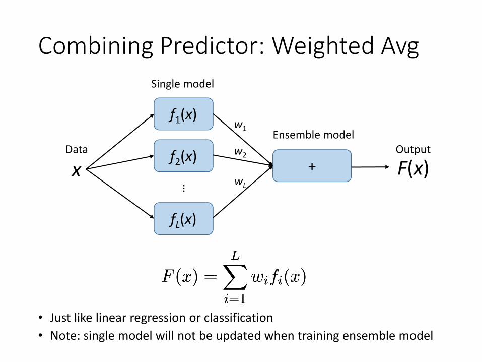
Combining Predictor: Weighted Avg
• Just like linear regression or classification• Note: single model will not be updated when training ensemble model
x
f1(x)
f2(x)
fL(x)
…
+ F(x)Data
Single model
Ensemble modelOutput
w1
w2
wL
F (x) =LX
i=1
wifi(x)F (x) =LX
i=1
wifi(x)
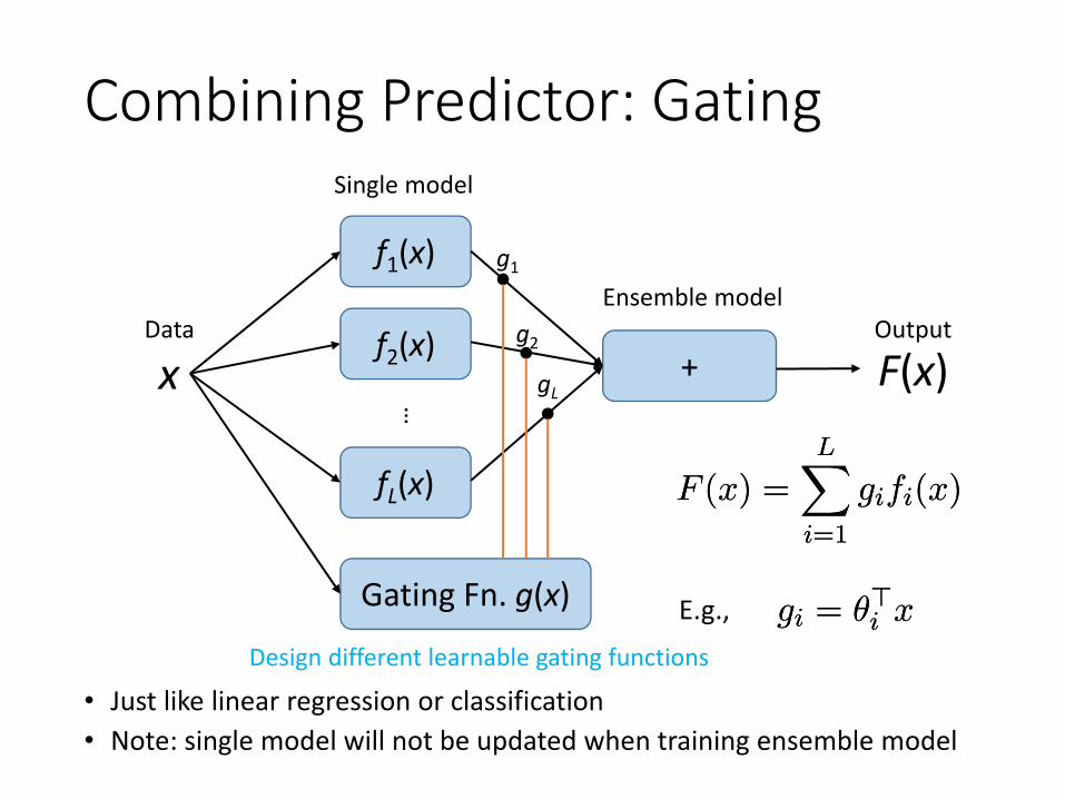
Combining Predictor: Gating
• Just like linear regression or classification• Note: single model will not be updated when training ensemble model
x
f1(x)
f2(x)
fL(x)
…
+ F(x)Data
Single model
Ensemble modelOutput
g1
g2
gL
Gating Fn. g(x)
F (x) =LX
i=1
gifi(x)F (x) =LX
i=1
gifi(x)
gi = μ>i xgi = μ>i xE.g.,Design different learnable gating functions
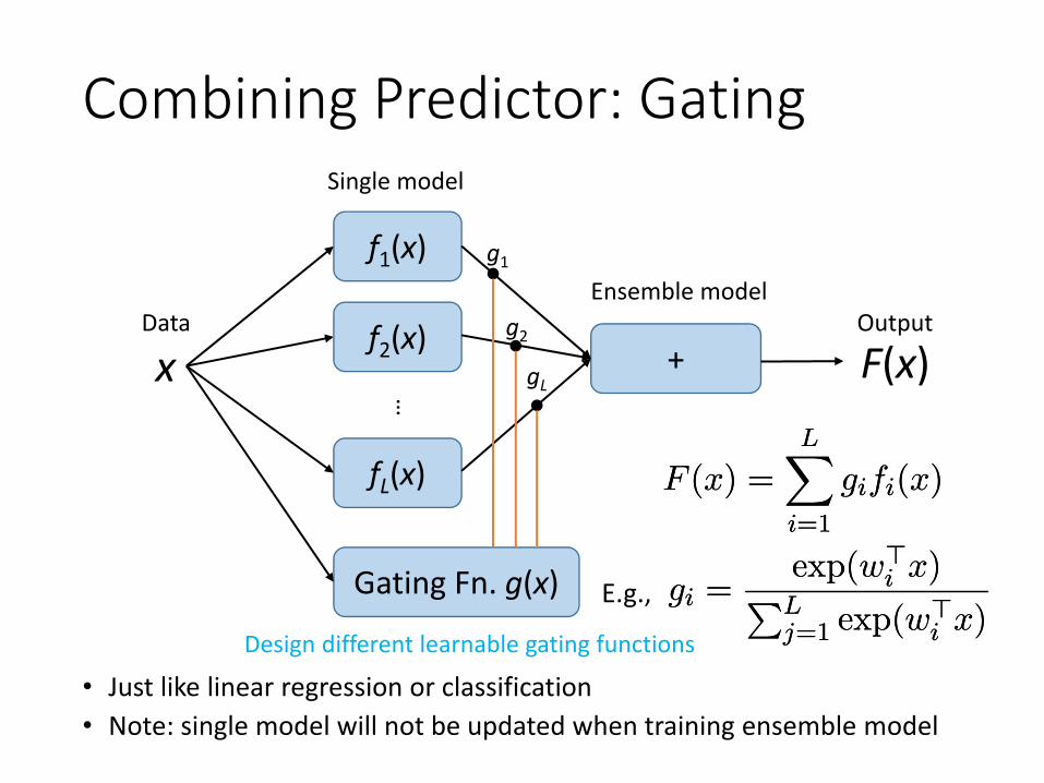
Combining Predictor: Gating
• Just like linear regression or classification• Note: single model will not be updated when training ensemble model
x
f1(x)
f2(x)
fL(x)
…
+ F(x)Data
Single model
Ensemble modelOutput
g1
g2
gL
Gating Fn. g(x)
F (x) =LX
i=1
gifi(x)F (x) =LX
i=1
gifi(x)
gi =exp(w>
i x)PLj=1 exp(w>
i x)gi =
exp(w>i x)PL
j=1 exp(w>i x)
E.g.,
Design different learnable gating functions
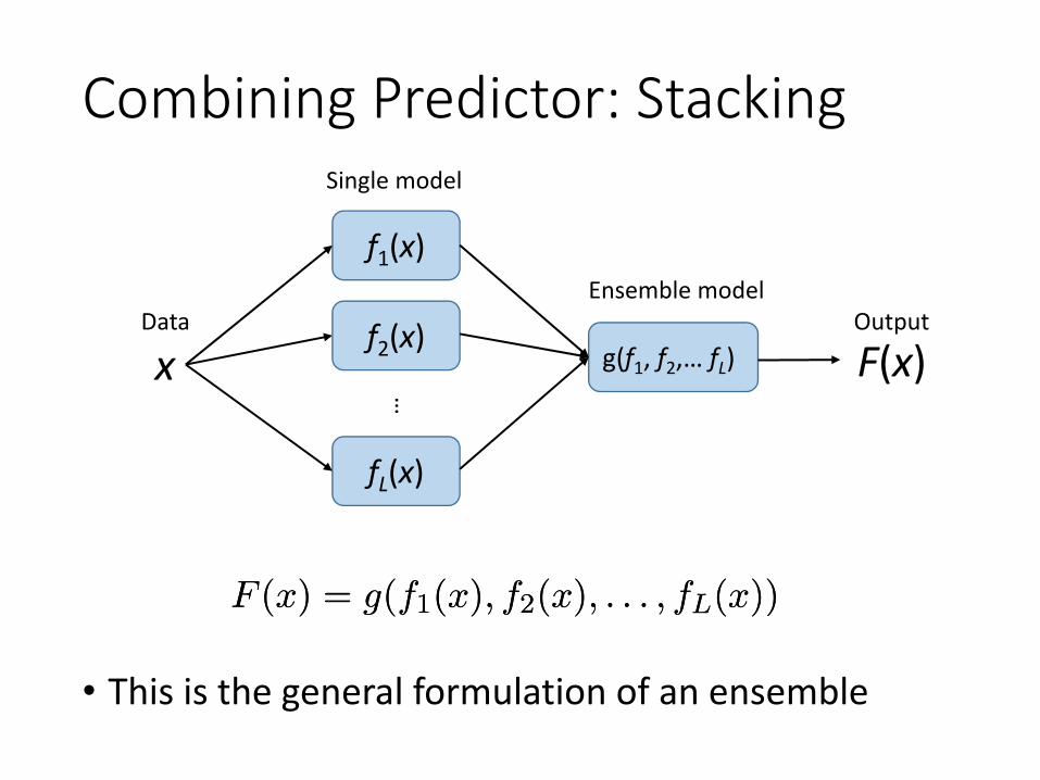
Combining Predictor: Stacking
• This is the general formulation of an ensemble
x
f1(x)
f2(x)
fL(x)
…
g(f1, f2,… fL) F(x)Data
Single model
Ensemble modelOutput
F (x) = g(f1(x); f2(x); : : : ; fL(x))F (x) = g(f1(x); f2(x); : : : ; fL(x))
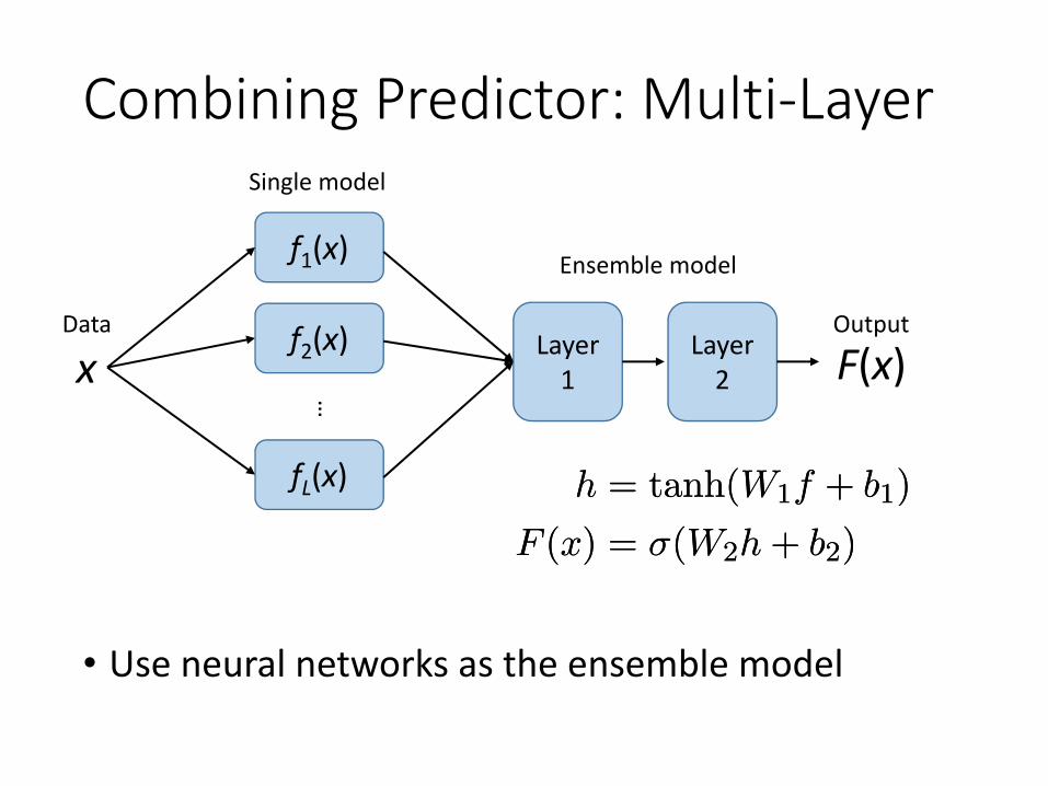
Combining Predictor: Multi-Layer
• Use neural networks as the ensemble model
x
f1(x)
f2(x)
fL(x)
…
Layer 1 F(x)
Data
Single model
Ensemble model
OutputLayer
2
h = tanh(W1f + b1)
F (x) = ¾(W2h + b2)
h = tanh(W1f + b1)
F (x) = ¾(W2h + b2)
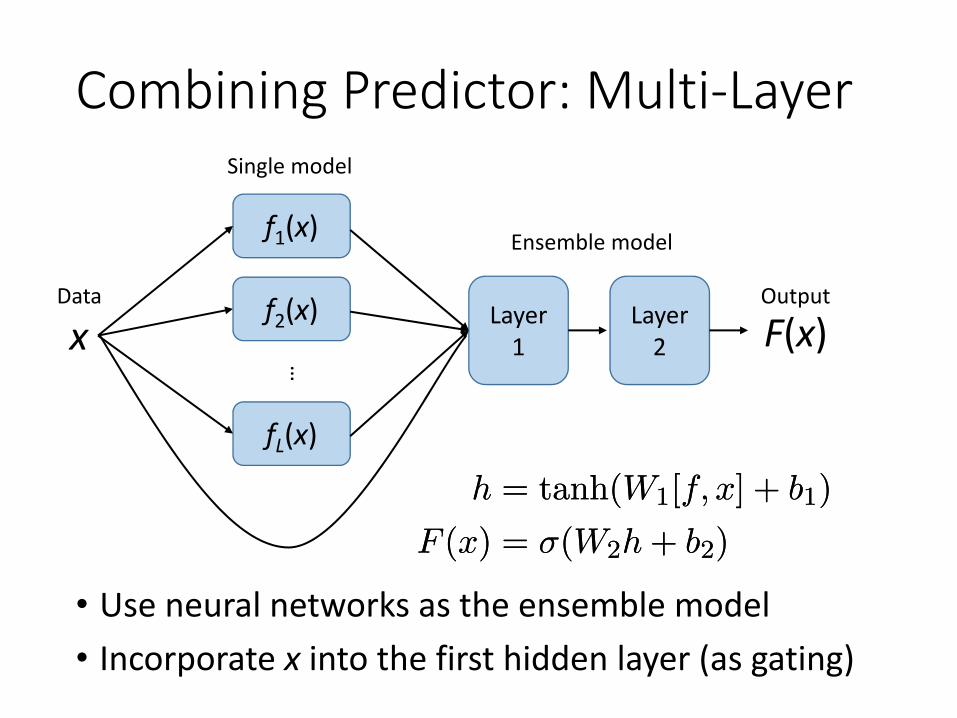
Combining Predictor: Multi-Layer
• Use neural networks as the ensemble model• Incorporate x into the first hidden layer (as gating)
x
f1(x)
f2(x)
fL(x)
…
Layer 1 F(x)
Data
Single model
Ensemble model
OutputLayer
2
h = tanh(W1[f; x] + b1)
F (x) = ¾(W2h + b2)
h = tanh(W1[f; x] + b1)
F (x) = ¾(W2h + b2)
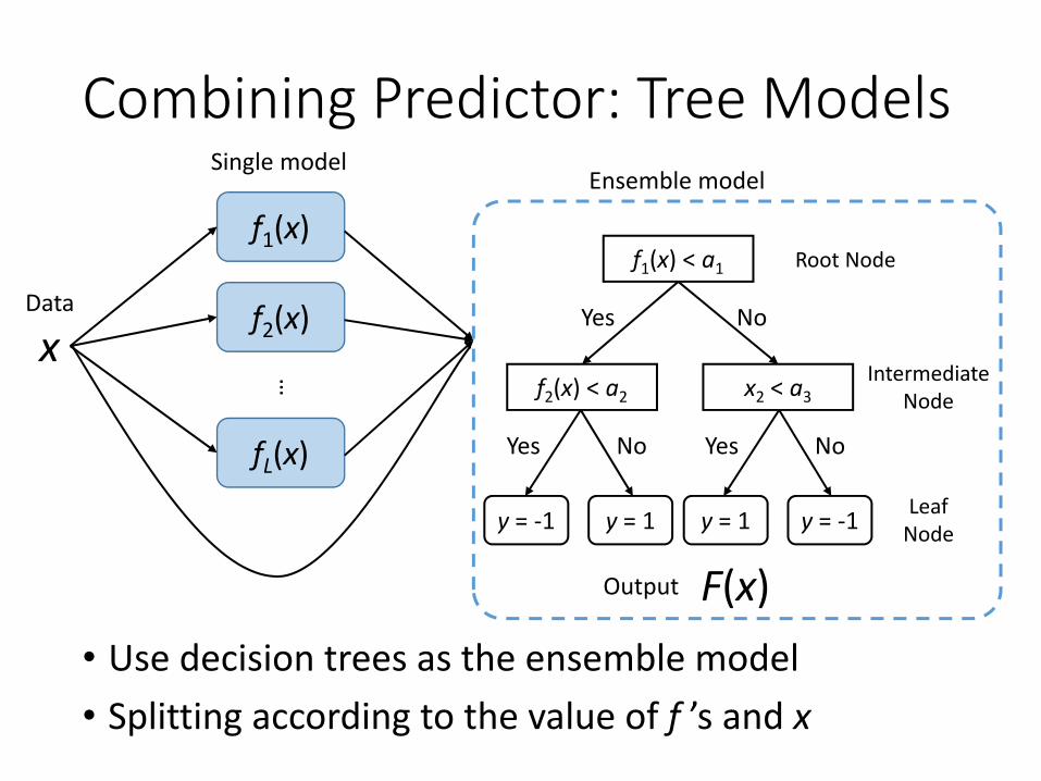
f1(x) < a1
f2(x) < a2 x2 < a3
Yes No
Yes No Yes No
IntermediateNode
LeafNode
Root Node
y = -1 y = 1 y = 1 y = -1
Combining Predictor: Tree Models
• Use decision trees as the ensemble model• Splitting according to the value of f ’s and x
x
f1(x)
f2(x)
fL(x)
…
F(x)
Data
Single modelEnsemble model
Output
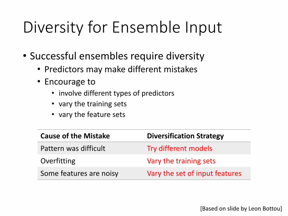
Diversity for Ensemble Input• Successful ensembles require diversity
• Predictors may make different mistakes• Encourage to
• involve different types of predictors• vary the training sets• vary the feature sets
[Based on slide by Leon Bottou]
Cause of the Mistake Diversification StrategyPattern was difficult Try different modelsOverfitting Vary the training setsSome features are noisy Vary the set of input features
BaggingRandom Forest
Ensemble Learning
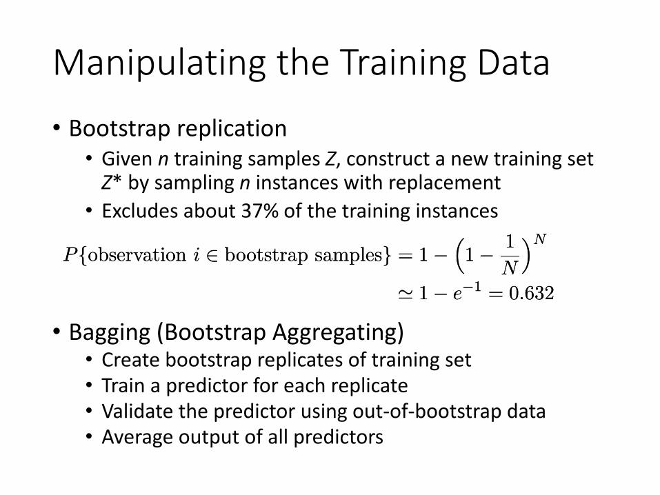
Manipulating the Training Data• Bootstrap replication
• Given n training samples Z, construct a new training set Z* by sampling n instances with replacement
• Excludes about 37% of the training instances
Pfobservation i 2 bootstrap samplesg = 1¡³1¡ 1
N
´N
' 1¡ e¡1 = 0:632
Pfobservation i 2 bootstrap samplesg = 1¡³1¡ 1
N
´N
' 1¡ e¡1 = 0:632
• Bagging (Bootstrap Aggregating)• Create bootstrap replicates of training set• Train a predictor for each replicate• Validate the predictor using out-of-bootstrap data• Average output of all predictors
Bootstrap
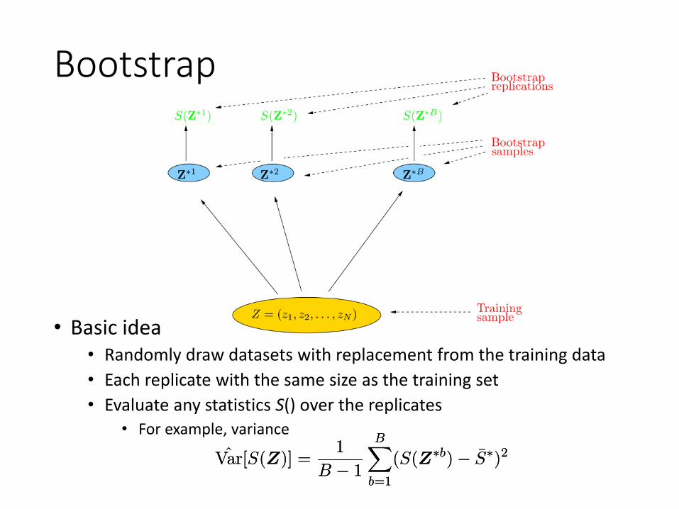
• Basic idea• Randomly draw datasets with replacement from the training data• Each replicate with the same size as the training set• Evaluate any statistics S() over the replicates
• For example, variance
Var[S(Z)] =1
B ¡ 1
BXb=1
(S(Z¤b)¡ ¹S¤)2Var[S(Z)] =1
B ¡ 1
BXb=1
(S(Z¤b)¡ ¹S¤)2
Bootstrap
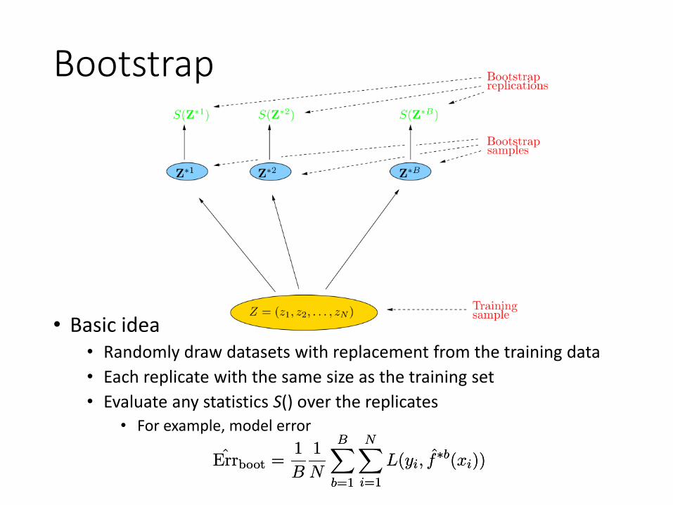
• Basic idea• Randomly draw datasets with replacement from the training data• Each replicate with the same size as the training set• Evaluate any statistics S() over the replicates
• For example, model error
Errboot =1
B
1
N
BXb=1
NXi=1
L(yi; f¤b(xi))Errboot =
1
B
1
N
BXb=1
NXi=1
L(yi; f¤b(xi))

Bootstrap for Model Evaluation• If we directly evaluate the model using the whole training
dataErrboot =
1
B
1
N
BXb=1
NXi=1
L(yi; f¤b(xi))Errboot =
1
B
1
N
BXb=1
NXi=1
L(yi; f¤b(xi))
Pfobservation i 2 bootstrap samplesg = 1¡³1¡ 1
N
´N
' 1¡ e¡1 = 0:632
Pfobservation i 2 bootstrap samplesg = 1¡³1¡ 1
N
´N
' 1¡ e¡1 = 0:632
• As the probability of a data instance in the bootstrap samples is
• If validate on training data, it is much likely to overfit• For example in a binary classification problem where y is indeed
independent with x• Correct error rate: 0.5• Above bootstrap error rate: 0.632*0 + (1-0.632)*0.5=0.184

Leave-One-Out Bootstrap• Build a bootstrap replicate with one instance i out,
then evaluate the model using instance i
Err(1)
=1
N
NXi=1
1
jC¡ijX
b2C¡i
L(yi; f¤b(xi))Err
(1)=
1
N
NXi=1
1
jC¡ijX
b2C¡i
L(yi; f¤b(xi))
• C-i is the set of indices of the bootstrap samples b that do not contain the instance i
• For some instance i, the set C-i could be null set, just ignore such cases
• We shall come back to the model evaluation and select in later lectures.
Bootstrap for Model Parameters• Sec 8.4 of Hastie et al. The elements of statistical
learning.
• Bootstrap mean is approximately a posterior average.
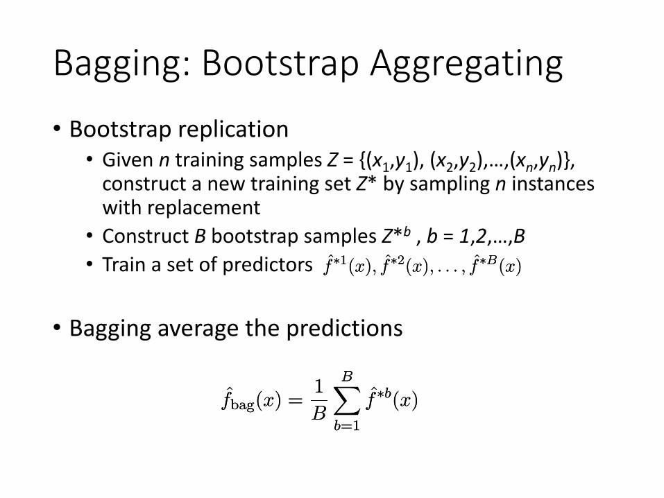
Bagging: Bootstrap Aggregating• Bootstrap replication
• Given n training samples Z = {(x1,y1), (x2,y2),…,(xn,yn)}, construct a new training set Z* by sampling n instances with replacement
• Construct B bootstrap samples Z*b , b = 1,2,…,B• Train a set of predictors
• Bagging average the predictions
fbag(x) =1
B
BXb=1
f¤b(x)fbag(x) =1
B
BXb=1
f¤b(x)
f¤1(x); f¤2(x); : : : ; f¤B(x)f¤1(x); f¤2(x); : : : ; f¤B(x)
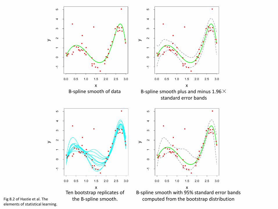
B-spline smooth of data B-spline smooth plus and minus 1.96×standard error bands
Ten bootstrap replicates of the B-spline smooth.
B-spline smooth with 95% standard error bands computed from the bootstrap distributionFig 8.2 of Hastie et al. The
elements of statistical learning.
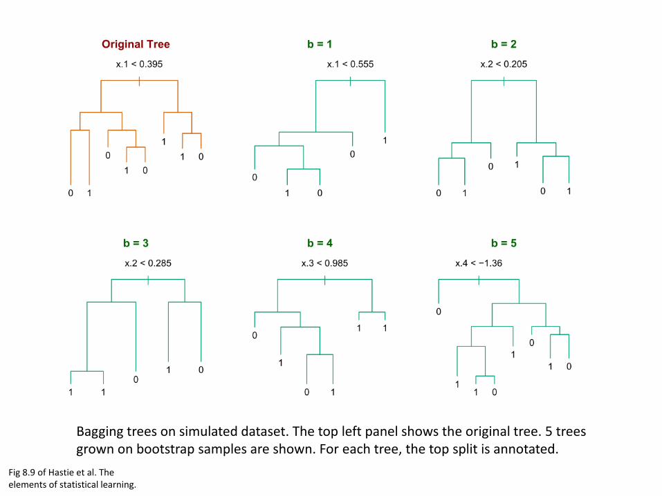
Fig 8.9 of Hastie et al. The elements of statistical learning.
Bagging trees on simulated dataset. The top left panel shows the original tree. 5 trees grown on bootstrap samples are shown. For each tree, the top split is annotated.
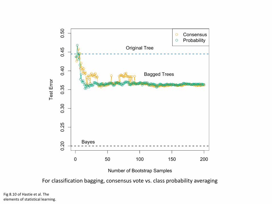
Fig 8.10 of Hastie et al. The elements of statistical learning.
For classification bagging, consensus vote vs. class probability averaging
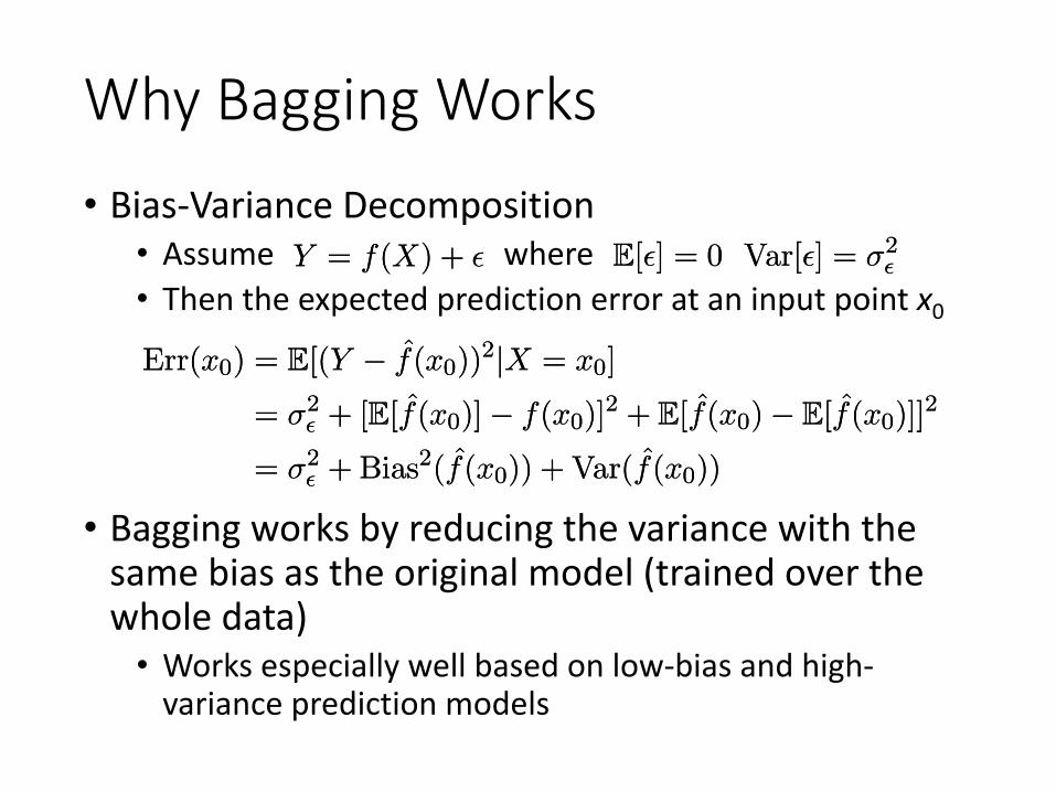
Why Bagging Works• Bias-Variance Decomposition
• Assume where• Then the expected prediction error at an input point x0
Y = f(X) + ²Y = f(X) + ² E[²] = 0 Var[²] = ¾2²E[²] = 0 Var[²] = ¾2²
Err(x0) = E[(Y ¡ f(x0))2jX = x0]
= ¾2² + [E[f(x0)]¡ f(x0)]
2 + E[f(x0)¡ E[f(x0)]]2
= ¾2² + Bias2(f(x0)) + Var(f(x0))
Err(x0) = E[(Y ¡ f(x0))2jX = x0]
= ¾2² + [E[f(x0)]¡ f(x0)]
2 + E[f(x0)¡ E[f(x0)]]2
= ¾2² + Bias2(f(x0)) + Var(f(x0))
• Bagging works by reducing the variance with the same bias as the original model (trained over the whole data)
• Works especially well based on low-bias and high-variance prediction models

Random Forest
Ensemble LearningBagging
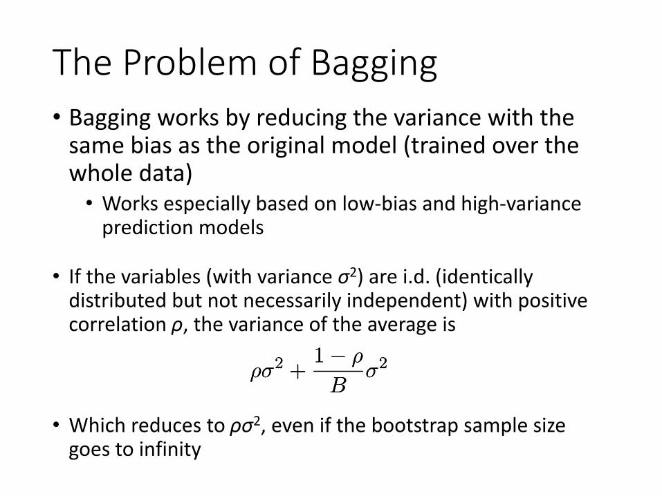
The Problem of Bagging
• If the variables (with variance σ2) are i.d. (identically distributed but not necessarily independent) with positive correlation ρ, the variance of the average is
• Bagging works by reducing the variance with the same bias as the original model (trained over the whole data)
• Works especially based on low-bias and high-variance prediction models
½¾2 +1¡ ½
B¾2½¾2 +
1¡ ½
B¾2
• Which reduces to ρσ2, even if the bootstrap sample size goes to infinity
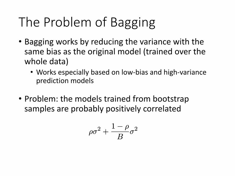
The Problem of Bagging
• Problem: the models trained from bootstrap samples are probably positively correlated
• Bagging works by reducing the variance with the same bias as the original model (trained over the whole data)
• Works especially based on low-bias and high-variance prediction models
½¾2 +1¡ ½
B¾2½¾2 +
1¡ ½
B¾2
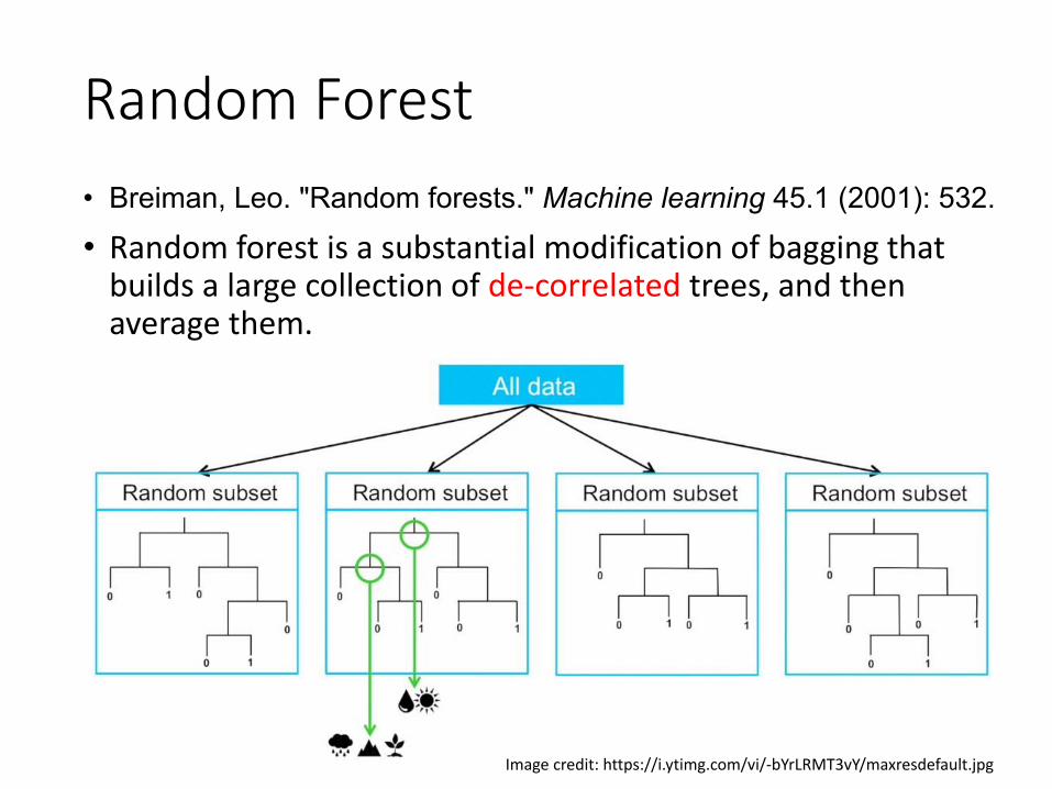
Random Forest• Breiman, Leo. "Random forests." Machine learning 45.1 (2001): 532.
• Random forest is a substantial modification of bagging that builds a large collection of de-correlated trees, and then average them.
Image credit: https://i.ytimg.com/vi/-bYrLRMT3vY/maxresdefault.jpg
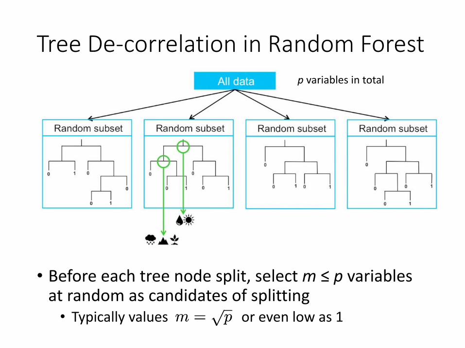
Tree De-correlation in Random Forest
• Before each tree node split, select m ≤ p variables at random as candidates of splitting
• Typically values or even low as 1 m =p
pm =p
p
p variables in total
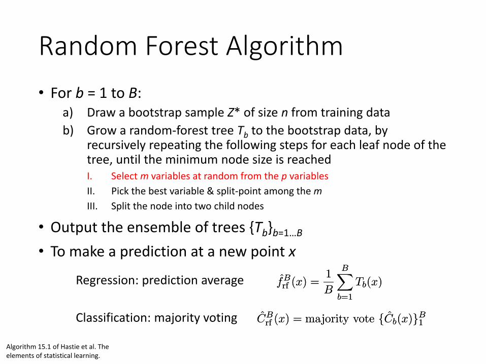
Random Forest Algorithm• For b = 1 to B:
a) Draw a bootstrap sample Z* of size n from training datab) Grow a random-forest tree Tb to the bootstrap data, by
recursively repeating the following steps for each leaf node of the tree, until the minimum node size is reachedI. Select m variables at random from the p variablesII. Pick the best variable & split-point among the mIII. Split the node into two child nodes
• Output the ensemble of trees {Tb}b=1…B
• To make a prediction at a new point x
Algorithm 15.1 of Hastie et al. The elements of statistical learning.
fBrf (x) =
1
B
BXb=1
Tb(x)fBrf (x) =
1
B
BXb=1
Tb(x)
Classification: majority voting
Regression: prediction average
CBrf (x) = majority vote fCb(x)gB
1CBrf (x) = majority vote fCb(x)gB
1
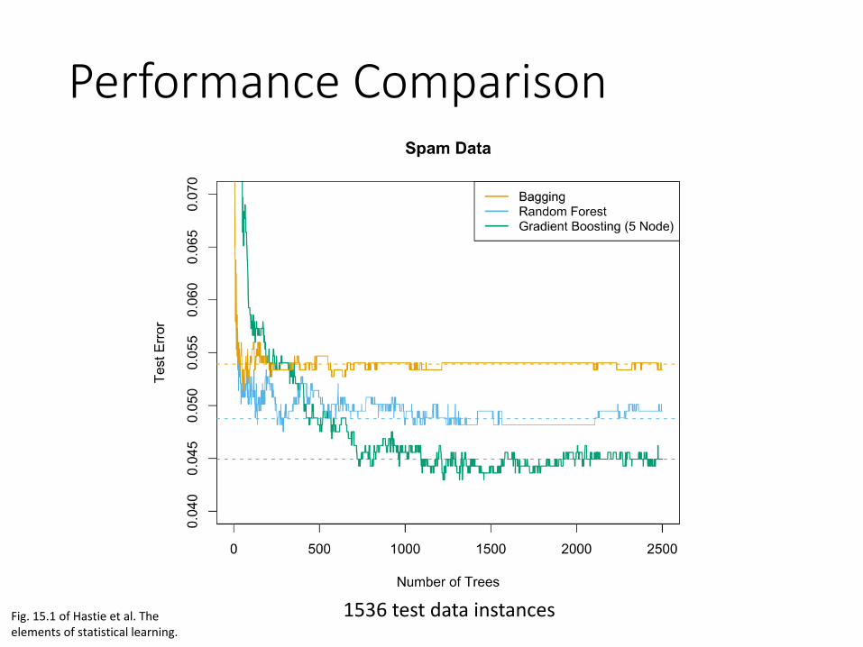
Performance Comparison
Fig. 15.1 of Hastie et al. The elements of statistical learning.
1536 test data instances
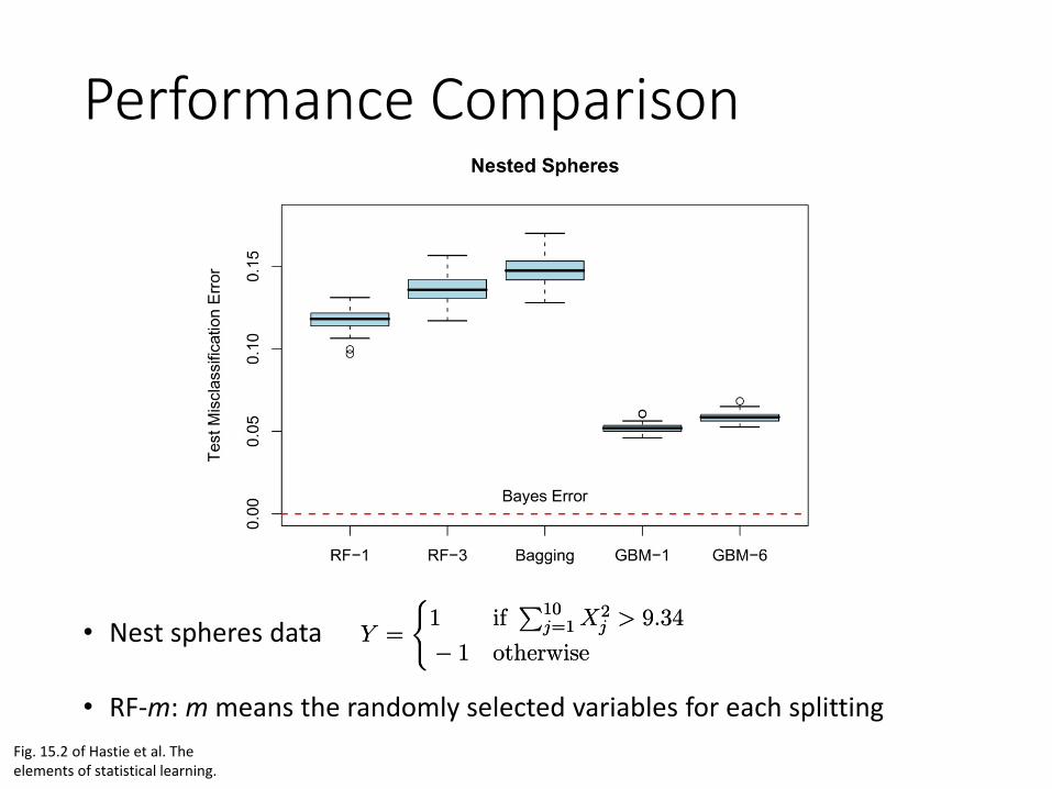
Performance Comparison
• RF-m: m means the randomly selected variables for each splittingFig. 15.2 of Hastie et al. The elements of statistical learning.
Y =
(1 if
P10j=1 X2
j > 9:34
¡ 1 otherwiseY =
(1 if
P10j=1 X2
j > 9:34
¡ 1 otherwise• Nest spheres data

CS420 Machine Learning
http://wnzhang.net/teaching/cs420/index.html
Course webpage:
Weinan Zhang
For more machine learning details, you can check out my machine learning course at Zhiyuan College


![Supervised and Semi-Supervised Deep Neural Networks for CSI-Based Authentication … · 2018. 7. 26. · arXiv:1807.09469v1 [cs.LG] 25 Jul 2018 Supervised and Semi-Supervised Deep](https://img.pdfslide.us/doc/110x75/60d0124181728b17c80222c4/supervised-and-semi-supervised-deep-neural-networks-for-csi-based-authentication.jpg)