Bachelor thesis

Supersymmetry and the Higgs sectorof the Next-to MinimalSuperSymmetric Model

Jacob Winding

Theoretical High Energy PhysicsDepartement of Astronomy and Theoretical Physics

Lund UniversitySolvegatan 14ASE-223 62 Lund

Supervised by: Johan Rathsman

Abstract

The problems of the standard model are reviewed and the motivations for in-troducing supersymmetry are discussed. The basic theory behind supersymmetryis described briefly, followed by an introduction of two realistic supersymmetricmodels; the Minimal SuperSymmetric Model (MSSM) and its proposed extension,the NMSSM. Some details of the NMSSM are stated and some constraints on pa-rameters are described. I then explore the Higgs boson masses and couplings forsome interesting scenarios, including a few different ways of taking the limit whereNMSSM reduces to MSSM.

1

Contents

1 Introduction 3

2 The Standard Model and supersymmetry 32.1 Review of the standard model . . . . . . . . . . . . . . . . . . . . . . . . . 32.2 Problems of the standard model . . . . . . . . . . . . . . . . . . . . . . . . 52.3 Motivation for supersymmetry . . . . . . . . . . . . . . . . . . . . . . . . . 6

3 Review of basic supersymmetry 73.1 The general supersymmetry algebra . . . . . . . . . . . . . . . . . . . . . . 93.2 General properties of supersymmetric theories . . . . . . . . . . . . . . . . 103.3 The D=4, N=1 SUSY algebra . . . . . . . . . . . . . . . . . . . . . . . . . 113.4 Representations of the algebra . . . . . . . . . . . . . . . . . . . . . . . . . 12

3.4.1 Representation of massive states . . . . . . . . . . . . . . . . . . . . 123.4.2 Massless states . . . . . . . . . . . . . . . . . . . . . . . . . . . . . 13

3.5 Superspace and superfields . . . . . . . . . . . . . . . . . . . . . . . . . . . 143.5.1 The chiral superfield . . . . . . . . . . . . . . . . . . . . . . . . . . 173.5.2 The vector superfield . . . . . . . . . . . . . . . . . . . . . . . . . . 18

3.6 Superspace integrals . . . . . . . . . . . . . . . . . . . . . . . . . . . . . . 193.7 Supersymmetric Lagrangians . . . . . . . . . . . . . . . . . . . . . . . . . . 20

3.7.1 Lagrangians for chiral superfields . . . . . . . . . . . . . . . . . . . 213.7.2 Supersymmetric, abelian gauge theory . . . . . . . . . . . . . . . . 22

3.8 Concluding remarks . . . . . . . . . . . . . . . . . . . . . . . . . . . . . . . 24

4 Realistic supersymmetric models 254.1 Softly breaking terms . . . . . . . . . . . . . . . . . . . . . . . . . . . . . . 254.2 The MSSM . . . . . . . . . . . . . . . . . . . . . . . . . . . . . . . . . . . 25

4.2.1 R-parity . . . . . . . . . . . . . . . . . . . . . . . . . . . . . . . . . 284.3 The NMSSM . . . . . . . . . . . . . . . . . . . . . . . . . . . . . . . . . . 29

5 Details of NMSSM 315.1 The mass matrices . . . . . . . . . . . . . . . . . . . . . . . . . . . . . . . 31

5.1.1 Neutral scalar states . . . . . . . . . . . . . . . . . . . . . . . . . . 325.1.2 CP-odd neutral states . . . . . . . . . . . . . . . . . . . . . . . . . 325.1.3 Charged states . . . . . . . . . . . . . . . . . . . . . . . . . . . . . 33

5.2 Reduced couplings . . . . . . . . . . . . . . . . . . . . . . . . . . . . . . . 335.3 Constraints on the parameters . . . . . . . . . . . . . . . . . . . . . . . . . 35

5.3.1 λ and κ . . . . . . . . . . . . . . . . . . . . . . . . . . . . . . . . . 355.3.2 tan β and Aκ . . . . . . . . . . . . . . . . . . . . . . . . . . . . . . 365.3.3 mH± and the other Higgs masses . . . . . . . . . . . . . . . . . . . 37

6 Results 376.1 Varying the charged Higgs mass . . . . . . . . . . . . . . . . . . . . . . . . 37

6.1.1 The NMSSM with a small κ . . . . . . . . . . . . . . . . . . . . . . 376.1.2 Larger κ . . . . . . . . . . . . . . . . . . . . . . . . . . . . . . . . . 396.1.3 A larger vs or µ-value . . . . . . . . . . . . . . . . . . . . . . . . . . 416.1.4 Large tan β values . . . . . . . . . . . . . . . . . . . . . . . . . . . 42

6.2 The MSSM limit . . . . . . . . . . . . . . . . . . . . . . . . . . . . . . . . 42

2

7 Summary and conclusions 46

1 Introduction

The standard model, despite being very successful and in overall very good agreement withexperiments, has many obvious shortcomings. One of the leading contenders claiming tosolve some of these is supersymmetry. As the perhaps most important example, we havethe problem of the small Higgs mass in the standard model, called the hierarchy problem,to be explained further later on. This problem is automatically solved in supersymmetrictheories, and there are many other problems which also goes away when we pass to asupersymmetric theory. From a theoretical viewpoint, supersymmetry is attractive notonly because it solves some problems, but also since it can be said to be the most generalpossible extension of our normal spacetime symmetries. In string theory, supersymmetryis also a required ingredient to get a consistent theory containing fermions.

One of the purposes with this study, which is a Bachelor thesis at Lund university, is togive a taste of how supersymmetry works and how some of the problems in the standardmodel are solved. The other, more practical, purpose is to take a closer look at the Higgssector in one of the proposed supersymmetric extensions of the standard model, and lookat some of its qualitative features.

This paper is structured as follows: We start by very quickly reviewing the standardmodel, followed by a discussion on its deficits. The next section is an attempt to motivatethe study of supersymmetry, which at first glance might seem slightly unrealistic but infact fixes many of the problems of the standard model in a fairly natural way. In thenext section, I try to introduce some basic concepts of supersymmetry at a hopefullyunderstandable level, adopting the superspace and superfield view of the theory. Thealgebra and some of its simplest representations is presented, the concepts of superspaceand superfields are introduced and finally some very simple global supersymmetric actionsare written down. After this the simplest realistic model incorporating supersymmetry,MSSM, is introduced, and some of its problems are discussed. The simplest possibleextension, NMSSM, which adds a singlet Higgs to the theory, is then proposed as a possiblesolution to the problems of MSSM, and the Higgs sector of this theory is studied in slightlymore detail. Then the next section presents some numerical results investigating the Higgsmass spectrum for different parameter choices and in the MSSM limit, and finally someconclusions from these results are stated.

2 The Standard Model and supersymmetry

In this section I will first very briefly describe the standard model of particle physics,followed by a discussion of its deficits and problems. Then I will argue that there is goodmotivation to study supersymmetry and describe how supersymmetric extensions of thestandard model solves some (although not all) of its problems.

2.1 Review of the standard model

The standard model (SM) is a highly successful theory of particle physics, and is overall consistent with all performed accelerator experiments (even though some precisionmeasurements seem to disagree, such as the anomalous magnetic moment of the muon).

3

Name Mass Spin Charge Isospin Iz (L/R)e− 0.511 MeV 1/2 -e −1

2/ 0

ν 0 < m < 2 eV 1/2 0 12

u 1.7-3.3 MeV 1/2 23e 1

2/ 0

d 4.1-5.8 MeV 1/2 −13e −1

2/ 0

γ m < 1× 10−18 eV 0 q < 1× 10−35e 0W± 80.40 GeV 1 ±1e 0Z 91.19 GeV 1 0 0

g (gluon) 0 1 0 0

Table 1: Properties of the particles in the first generation as well as the gauge bosons.Data taken from the Particle Data Group[1].

This section will be very brief, but there is of course a lot of reading material out there, sofor a more complete introduction see for example [2]. Concisely put, the standard modelis a relativistic quantum gauge field theory with gauge group SU(3) × SU(2) × U(1).The SU(2)×U(1) symmetry is spontaneously broken, leaving only the explicit remainingU(1) symmetry of electromagnetism, with the photon as the massless gauge boson. Thesymmetry breaking gives masses to the gauge bosons W±, Z which mediates the weakforce. In order to break the symmetry, there needs to be a scalar field, called the Higgsboson, that when it acquires a nonzero vacuum expectation value (VEV) breaks thesymmetry. It is through the couplings to this field that all particles acquire their mass.The SU(3) symmetry is left unbroken, and is carried by 8 massless gauge bosons calledthe gluons.

The remaining particles of the SM are all massive fermions, and seems to come “or-ganized” in three identical, except for masses, generations. In every generation there aretwo quarks that carry the SU(3) charge, commonly called colour, as well as two leptonswhich doesn’t carry colour. See table 1 for a summary of the particles in the first gener-ation, as well as the gauge bosons and some of their properties. A curious fact about thestandard model is that the weak force treats left and right handed fermions differently; itonly interacts with the left handed particles. Thus, we have to treat for example the lefthanded electron eL and the right handed eR differently, and the same for the quarks. Weorganize the particles so that the left handed particles sits in SU(2) doublets, whereas theright handed are SU(2) singlets. For the first generation the particles are

L =

(νeL

), Q =

(uLdL

), eR, uR, dR (1)

and analogously for the two other generations. The absence of a νR is due to the fact thatthe neutrino in the standard formulation is treated as massless and since the right handedneutrino doesn’t have any gauge couplings, there is no reason for including it. However,since the neutrinos are not really massless, only very light, it is possible that a νR has tobe added.

In a gauge theory such as the standard model, gauge symmetry doesn’t allow us todirectly add mass terms to the Lagrangian. This is solved by the idea of spontaneoussymmetry breaking, where the vacuum becomes non-symmetric. In order to do this inthe standard model, we add the Higgs field, which is a SU(2) doublet of complex scalarfields, and carries no colour. The parameters of the potential of this new field can then bechosen such that, in unitary gauge the stable minimum is one where the lower component

4

of the doublet acquires a nonzero vacuum expectation value (VEV). This vacuum is notsymmetric under the electroweak symmetry group SU(2)×U(1), but is symmetric undera (different) U(1) symmetry. This is the U(1) of electromagnetism, and we say that theelectroweak symmetry has been spontaneously broken. Further, since the Z and the W±

(which really are the linear combinations of the original gauge bosons of the unbrokenelectroweak symmetry that couples to the Higgs field) couple to the Higgs field and thusto its nonzero VEV, this gives them an effective mass term. In the same way we can addYukawa couplings between the Higgs field and the massive fermions of the theory, givingthem effective mass terms. That part of the standard model Lagrangian is called theYukawa sector and is where most of the free parameters (the Yukawa coupling strengths,giving the masses) enters. An introduction at a very readable level to more exactly howthe Higgs mechanism works can be found in [2], and for a slightly more technical reviewalso discussing supersymmetry and technicolor ideas, see [3].

2.2 Problems of the standard model

The standard model, while highly successful and in good agreement with the absolute ma-jority of performed experiments (there are however some persistent measured deviations,like the anomalous magnetic moment for the muon), still has some serious problems andis theoretically very unsatisfactory. For one thing, it has a large number (at least 19) ofarbitrary parameters, including the particle masses, the three gauge couplings, the weakmixing angles and the CP-violating Kobayashi-Maskawa phase. Since it appears thatneutrinos are not as previously believed massless, one must to the above ∼ 19 parametersadd three neutrino masses, three neutrino mixing angles and three different CP-violatingphases. And to describe how the neutrinos acquire mass in a realistic way, even moreparameters are necessary.

Another obvious deficit of the standard model is that it doesn’t describe the fourthknown force, gravity. What one would ultimately want is a theory that describes all theknown forces in a unified way.

Other things that are observed but not described by the standard model is the largebaryon asymmetry, i.e. why there is so much more matter than antimatter in the observeduniverse. There is a mechanism in the SM to create such an asymmetry but it is nowherenear strong enough to match what we observe. The large number of flavours in particlephysics, that there are so many types of quarks and leptons, why they seem to come ingenerations and why the weak interaction mixes these generations the way it does is alsoexamples of things that have no good explanations in the standard model.

The standard model also has to be modified in order to be consistent with the standardtheories of cosmology. Especially, it cannot explain the observed cold dark matter, andwhen one calculates the vacuum energy in the standard model it gives contributions thatare far too large to match the observed small, but nonzero, value of the cosmologicalconstant. Another problem is that the standard model needs to be modified in order tobe consistent with inflation.

Then there is the “hierarchy problem” concerning the smallness of gravity comparedto electromagnetism. Since gravity couples to mass, this problem is equivalent to askingwhy the particle masses are so much smaller than the Planck mass scale (MP ∼ 1019

GeV), i.e. why the ratio of the electroweak scale (∼MW ) and the Planck scale is so tiny,MW/MP ∼ 10−16. From reasons stated above, we know that the standard model is aneffective theory, at most valid up to the Planck scale. This means that when renormalizing

5

the theory we must have a finite energy cutoff, that can at largest be the Planck mass.This finite cutoff is really what causes the problem. The masses of the particles comefrom the Higgs mechanism, so the question why the masses of the particles are small isin turn equivalent to asking why the Higgs has such a small mass. If one calculates loopcorrections to the Higgs propagator, one finds that the corrections look like

δm2H h O(α)Λ2,

so the correction to the mass squared are proportional to the square of the UV-cutoff Λ,which by our previous reasoning is some large, finite energy, maybe of order MP or atleast of some large unification scale (called the GUT-scale, for Grand Unified Theory). Soin order to give the Higgs its required mass, which of course is much smaller than either ofthese scales, these loop corrections has to be very precisely cancelled. This we can do bygiving the tree level diagram exactly the required value. Technically, this is not a problemsince there is no constraint on the value of the bare mass, but it introduces a very heavyfine-tuning into the theory, where the bare mass has to have exactly the correct value,and this is theoretically very unsatisfying.

A thing to note is that implicit in this line of reasoning is that you assume that there isno need for new physics below some very large energy, i.e. the cutoff scale is large. This iscalled the “big desert” assumption, and while many, holds this to be true, not all physicistsagree. An argument for this assumption is that in the standard model, the running ofthe couplings is such that at a high energy scale, the grand unified scale (GUT-scale),of about ∼ 1016 GeV, all the known coupling become roughly the same, which impliesthat at least at this scale, our current physics should drastically change. Supersymmetryactually improves this a bit, making the couplings meet more closely than in the standardmodel. If one accepts the big-desert assumption, then the hierarchy problem is real, andsome mechanism is needed to keep the Higgs mass small. Supersymmetry is the mostpopular proposal to solve this problem, but other theories exists, such as technicolor[4, 5] (in which the Higgs is a composite particle) and extra dimensions (for example theADD model[6]). In the next section I will briefly explain how supersymmetry solves thehierarchy problem.

A final problem worth mentioning briefly is the strong CP problem. This comes fromthe observational fact that the strong interaction as described by QCD doesn’t seem toviolate CP symmetry, in contrast with the weak force. This is a problem since there arenatural terms in the QCD Lagrangian that violates CP conservation. To conform to theexperimental data, a large amount of fine-tuning is again required. The most well-knownproposition for solving this problem introduces new scalar particles, called axions, whichcan make an appearance in the NMSSM, as discussed later.

2.3 Motivation for supersymmetry

So what is supersymmetry and why would we want it? What it is, is a symmetry relatingfermions to bosons, requiring that every particle has a supersymmetric partner with thesame quantum numbers only differing in spin by 1/2. Since none of the known particlesonly differs in spin from another known particle, it might seem like a really bad idea tointroduce a symmetry that more than doubles (we need at least one extra Higgs doublet,why is explained later) the number of particles needed. But despite this, there is still somecompelling reasons for studying supersymmetric theories. From a phenomenological pointof view, perhaps one of the stronger arguments is that supersymmetry (SUSY) offers a

6

good candidate for dark matter, since it turns out that the lightest supersymmetric partner(which is a mixture of the superpartners of the photon, Z-boson and neutral Higgs bosons,called the neutralino) has to be stable, if we assume R-parity (which in turn is stronglyimplied from limits on the proton lifetime).

A slightly more theoretical argument concerns the gauge coupling unification at somehigh energy. In the usual standard model, the couplings run in such a way that theyalmost, but not exactly, all reach the same value at a high energy. Introducing SUSYgives exactly the contributions needed to make all the couplings meet.

Another attractive feature of supersymmetry is that it offers a way of constructinga theory of quantum gravity. The “ordinary” supersymmetry which we will study inthis paper is a global symmetry, but if you gauge it, i.e. make it local, you necessarilyget a theory of gravity, called supergravity[7]. Since, as we will see, supersymmetry is anextension of the ordinary spacetime symmetries rather than a new internal symmetry, it isnatural to see how curved spacetime and thus gravity follows from a local supersymmetry.

As mentioned above, one other good reason to investigate supersymmetry is that itsolves the hierarchy problem. Supersymmetry solves it since for every fermion that cou-ples to the Higgs, it adds a scalar with the same quantum numbers. When calculatingthe loop corrections, the fermion loops and the scalar loops will be of the opposite signand (if supersymmetry wasn’t broken) be of the same size and thus cancel. Even whensupersymmetry is broken, this removes the dependence on Λ2 and reduces it to a loga-rithmic divergence[8], if supersymmetry is softly broken. It is worth pointing out that theproblem isn’t really the quadratic dependence but rather that we have good reasons tobelieve that the standard model only is valid up to some finite energy scale. This meansthat we cannot just send Λ to infinity and then remove the infinity in the Higgs mass byour usual renormalization methods. Instead we can only send Λ to some GUT-scale, sincewe expect the standard model to only be valid up to that scale. So if one believes thatthe standard model breaks down well before reaching the GUT-scale, in principle there isno problem. However we have no good theoretical or experimental reason to believe thisto be the case, so the hierarchy problem remains.

Supersymmetry also lowers the vacuum energy you get from your quantum field theory,but nowhere near enough to explain the small cosmological constant. In fact, as is shownlater, exact supersymmetry requires the cosmological constant to be exactly zero. Yetanother reason is that string theory, which is one of the leading candidates for a “theoryof everything” demands at least some kind of supersymmetry in order to consistentlycontain fermions.

However compelling these argument may seem, there is as of now no direct experimen-tal indication that the world is supersymmetric. Since we do not see all the supersym-metric partners, it is obvious that they do not have the same mass, so if supersymmetryindeed is a symmetry of nature, it must be broken. Then one can ask, in what way is itbroken and what is the breaking scale?

Supersymmetry has grown into a vast field, and the purpose of this section is merelyto give the reader a flavour of the exciting ideas involved. For more complete expositions,there are numerous books and articles to consult, for example [9, 10, 11, 12].

3 Review of basic supersymmetry

In this section, I will briefly go through some of theory behind supersymmetry, statingthe simplest possible algebra, look at its particle representations, introduce the concept

7

of superspace and superfields, and finally look at how to use these concepts in order towrite down a supersymmetric Lagrangian. Beware that this is a large and deep subjectthat branches of into many different areas of theoretical physics, and this brief review willonly scratch the surface.

With that said, lets start by looking at how to characterize supersymmetry. In ordinaryparticle physics, we have three different kinds of symmetries:

• Poincare invariance, or spacetime symmetry, i.e. symmetry under boosts, rotationsand translations. This is generally described by the Poincare algebra (which basi-cally describes how “infinitesimal symmetry transformations”, i.e. the generators,commute, like for example the relation [Ji, Jk] = εijkJk of rotation generators inquantum mechanics).

• Internal symmetries, for example the SU(2) × U(1) for the electroweak theory, orSU(3) for the strong force. These are local gauge symmetries, and their generators allcommute with the Poincare generators, which explains the name internal symmetriessince they live in their own internal spaces without mixing with spacetime itself.

• The discrete symmetries C (charge conjugation), P (parity) and T (time reversal).In the standard model only the combination of all of them, CPT, is a real symmetry,and there is a theorem saying that this must be the case in any quantum field theory.

There is a famous theorem by Coleman and Mandula[13] that proves that under certainreasonable conditions these are all the possible symmetries we can have. In particular,it is not possible to extend the spacetime symmetry by adding new symmetry generatorswith non-vanishing commutators with the Poincare group generators. However, one ofthe implicit assumptions of the theorem is that the algebra of the symmetry only involvesnormal commutators, or put in another way, that all generators are bosonic. It turnsout that we can enlarge the symmetry by allowing the added generators to instead beanticommuting, or fermionic. Supersymmetry is then defined by introducing anticommut-ing symmetry generators which transforms in the (1

2, 0) and (0, 1

2) representation of the

Lorentz group, that is in the left and right handed Weyl spinor representation. Alreadyhere we see that since these generators are not scalar, they transform non-trivially underLorentz transformations and are thus not the same as an additional internal symmetry.

In fact, in 1975, Haag Lopuszanski and Sohnius [14] proved that supersymmetry isthe most general symmetry allowed when including anticommutating generators. Onemight then think that further weakening of assumptions might lead to more interestingsymmetries, but so far no compelling example of such a symmetry has been found. Thus,we can make a strong but not entirely unreasonable assertion that supersymmetry is theonly possible extension of the ordinary spacetime symmetries.

Notational conventions

I here introduce some notation we need for stating the algebra and supersymmetric theo-ries in a nice and clean way. For a left handed Weyl spinor with two components we willwrite ψα where α = 1, 2 is a left handed spinor index, and for a right handed spinor I writeψα, where the dot indicates a right handed spinor index. The conjugate of a left handedspinor is a right handed, ψα = (ψα)†. We use the two dimensional fully antisymmetricLevi-Civita symbols to lower and raise spinor indices, where ε12 = −1 and ε12 = 1. Forexample

ψα = εαβψβ, ψα = εαβψβ

8

and so on. Another definition that is needed to state the algebra in this formalism is ofthe matrices

σµ = (1, ~σ) = σµ (2)

σµ = (1,−~σ) = σµ (3)

where 1 denotes the 2 × 2 identity matrix, ~σ is the ordinary Pauli matrices and µ is aLorenz index taking values 0, 1, 2, 3. Note that the bar here is part of the name and doesn’timply any kind of conjugation. Also note that in these conventions, the unbarred σ carriesone undotted and one dotted index: σµ

αβ, whereas the barred has dotted-undotted indices:

σµαβ.We also need the Lorentz generators for left and right handed Weyl spinors, which are

basically the commutators of σµ and σν ,

(σµν)αβ =

1

4

(σµαγσ

νγβ − (µ↔ ν))

(4)

(σµν)α β =1

4

(σµαγσν

γβ− (µ↔ ν)

)(5)

Note here that σ12 = σ12 = −12σ3 so that the rotation generator M12 = 1

2σ3, as usual. As

a warning to the reader, in the literature there are many different conventions for how todefine various quantities, so these used here are in no way standard. In this study, we willfollow the conventions of [10].

3.1 The general supersymmetry algebra

So we enlarge the Poincare algebra with either left or right handed spinor generators, QIα

or QIα where I = 1, . . . , N labels the different pairs of generators in case we add more than

one pair. The new generators should commute with the translation generators, which isnot directly obvious but can be shown using Jacobi relations, so

[QIα, Pµ] = [QI

α, Pµ] = 0. (6)

The fact that the added generators are spinors dictates how they transform under Lorentztransformations and thus their commutation relations with the generators Mµν of theLorentz transformations are

[QIα,Mµν ] = σβµναQ

Iβ , (7)

[QIα,Mµν ] = σαµνβ

QIβ . (8)

Since QI is in the (12, 0) representation and QI is in the (0, 1

2), the anticommutator

QI , QI must be in the (12, 1

2), i.e. a fourvector. The natural candidate is Pµ. Further, by

rotating the differentQI generators, and rescaling them, we can always let QI , QJ ∝ δIJ ,so the anticommutation relation becomes

QIα, Q

Jβ = 2δIJσµ

αβPµ . (9)

Then, we can also take the anticommutator between QIα and QJ

β . Generally, we have forthese

QIα, Q

Jβ = εαβZ

IJ ,

QIα, Q

Jβ = εαβ(ZIJ)∗ . (10)

9

The ZIJ are called the central charges, central because they commute with all the gener-ators in the algebra. Because of the antisymmetric ε and the symmetry of the anticom-mutator, we must have ZIJ = −ZJI , so we see that with only one extra generator, N = 1they must vanish because of this antisymmetry. This is obviously the simplest case, andis what we will study in slightly more detail in a later section. But first, one can notesome general properties from the general algebra.

3.2 General properties of supersymmetric theories

Using the SUSY algebra, it is relatively easy to deduce some basic and general properties ofsupersymmetric theories. For one thing, since the usual Poincare algebra is a subalgebra,an irreducible representation (irrep) of the full supersymmetric algebra will also be arepresentation of the Poincare algebra, although not necessarily an irreducible one. Aswe will see, an irrep of the SUSY algebra will correspond to several different irreps of thePoincae algebra, i.e. several particles. We call the irreducible representation of the SUSYalgebra a supermultiplet, exactly because it contains multiple particles. The differentparticles in a supermultiplet are then related to each other through the action of QI andQJ .

Further, since M12 = 12σ3 ≡ S3, the spin (or helicity) operator in the x3 = z direction,

we have from the algebra above that [J3, QI1] = 1

2QI

1 and [S3, QI2] = −1

2QI

2, and the exactsame for QI

1, QI2. This means that QI

1 and QI1 raises the spin (helicity) in the z-direction

by half a unit, and that QI2, Q

I2 lowers it by half a unit. Combined with the reasoning

above, this means that the particles in an irrep of the supersymmetric algebra have spins(helicities) differing by units of one half. This also means, by the spin-statistics theorem,that the Q and Q generators change bosons into fermions and fermions into bosons.

Another thing that is easy to prove using the algebra is that PµPµ = P 2 = m2 is a

Casimir of the SUSY algebra. This means that it commutes with all the elements of thealgebra, and thus, by Schurs lemma, that is has to be a scalar quantity, i.e. a multipleof the identity. This has the consequence that all the particles in a supermultiplet musthave the same mass.

In a supersymmetric theory the energy (represented by P0) must be positive definite.This follows from the algebra since, if |Ω〉 is any state in the Hilbert room, which has apositive norm by definition, we have

0 ≤ |QIα|Ω〉|2 + |QI

α|Ω〉|2 = 〈Ω|QIαQ

Iα +QI

αQIα|Ω〉

= 〈Ω|QIα, Q

Iα|Ω〉 = 2σµαα〈Ω|Pµ|Ω〉. (11)

Taking the trace of this, i.e. summing over α = α = 1, 2 and using that all of the ~σ aretraceless, we have Tr σµ = 2δµ0, and we get

0 ≤ 4〈Ω|P0|Ω〉,

so the energy must be positive. This fact is very important when discussing the breakingof supersymmetry. In fact, it is easy to show that supersymmetry is spontaneously brokenif and only if the vacuum energy is positive. A natural question is to wonder why thevacuum energy should matter at all, why can’t we, as is usual when dealing with normalfield theories, just shift the zero point energy in order to make it exactly zero? This wecannot do because the energy now is dictated by our symmetry, since the Hamiltonianappears in the algebra.

10

Another property is that a supermultiplet always contains the same number of fermionicand bosonic degrees of freedom. The degrees of freedom here means the number of differ-ent physical states. For example, a real scalar field has one degree of freedom, a photonhas has two corresponding to its two helicities, and a spin 1/2 particle also has two cor-responding to its different possible spins. To prove this, assign a fermion number NF toeach state in a supermultiplet, where NF = 1 for a fermionic state and 0 for a bosonicstate. Equivalently, this means that (−1)NF = ∓1 for a fermionic respectively bosonicstate. Then the statement that a given supermultiplet has the same number of fermionicand bosonic states can be stated∑

states

(−1)NF = Tr(−1)NF = 0 , (12)

where the sum runs over all states in the supermultiplet (which is the same as taking thetrace over the representation). Since the supercharge Q turns bosons into fermions andvice versa, we have (−1)NFQ = −Q(−1)NF , that is, they anticommute. This we can use,by choosing some nonzero momentum pµ and computing

0 = Tr((−1)NF QβQα − (−1)NF QβQα

)= Tr

((−1)NF QβQα −Qα(−1)NF Qβ

)= Tr

((−1)NF Qα, Qβ

)= 2σµ

αβTr((−1)NFPµ

), (13)

which since pµ is nonzero implies the desired result. In the second equality, I use thecyclicity of the trace, followed by using the anticommutation of Q and (−1)NF to get theanticommutator we need to use the algebra.

3.3 The D=4, N=1 SUSY algebra

The simplest of all possible supersymmetries in four dimensions are when we only addone new fermionic generator, this is known as D = 4, N = 1 supersymmetry. In thiscase there can be no central charges because of the fact that they are antisymmetricso Z11 = −Z11 = 0. The addition of multiple new generators and central charges dointroduce some new things, but to discuss realistic supersymmetric models as we shall dohere, it is enough to talk about N = 1. In fact, N = 1 is the only case that can be usedas a simple low-energy extension of the standard model. This is because when N > 1there is no supermultiplet containing only left or righthanded fermions, which we needsince the weak force interacts differently with left and righthanded particles. Of course,at high enough energy we could still have a theory with N = 2 or higher, but then thissymmetry has to be broken so that only a N = 1 supersymmetry remains closer to theelectroweak scale.

The algebra in glorious detail is

Qα, Qβ = 2σµαβPµ (14)

Qα, Qβ = Qα, Qβ = 0 (15)

[Qα, Pµ] = [Qα, Pµ] = 0 (16)

[Qα,Mµν ] = σαµνβ

Qβ (17)

[Qα,Mµν ] = σβµναQβ. (18)

11

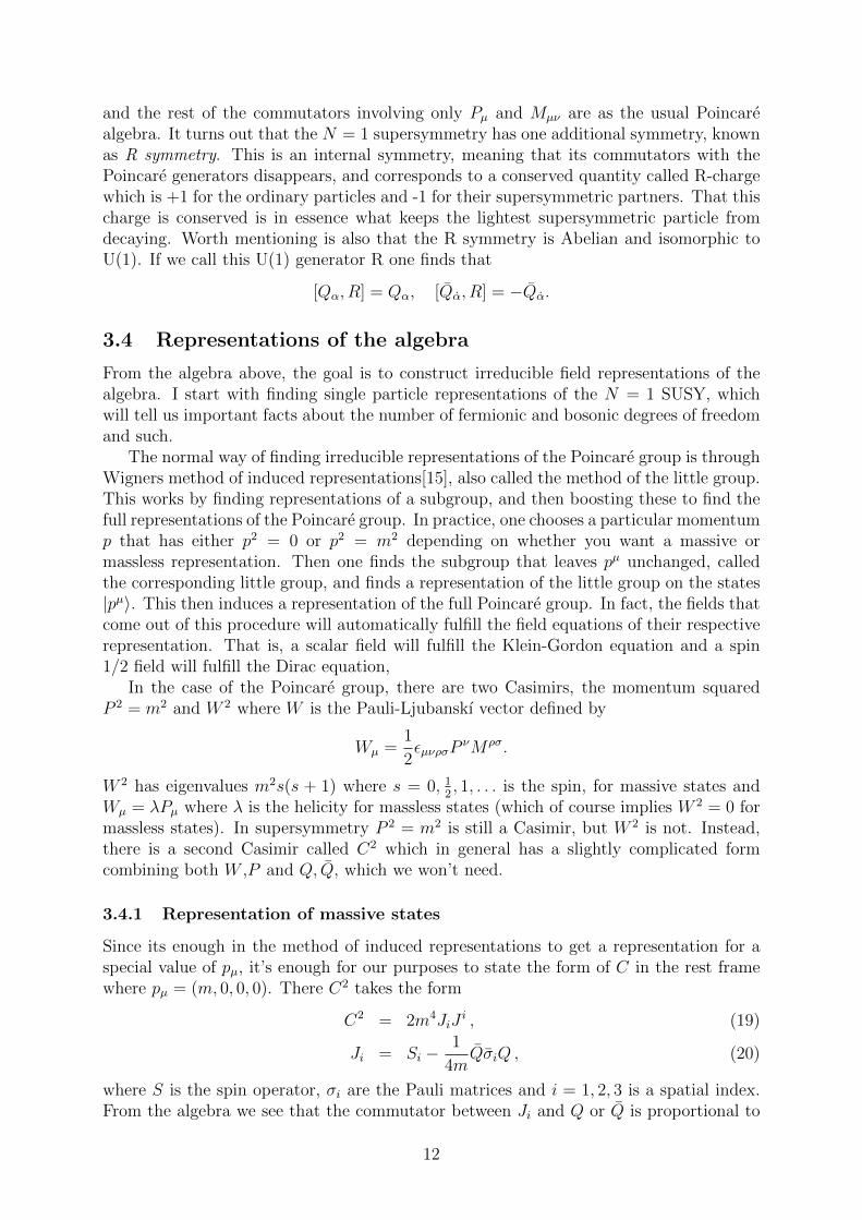
and the rest of the commutators involving only Pµ and Mµν are as the usual Poincarealgebra. It turns out that the N = 1 supersymmetry has one additional symmetry, knownas R symmetry. This is an internal symmetry, meaning that its commutators with thePoincare generators disappears, and corresponds to a conserved quantity called R-chargewhich is +1 for the ordinary particles and -1 for their supersymmetric partners. That thischarge is conserved is in essence what keeps the lightest supersymmetric particle fromdecaying. Worth mentioning is also that the R symmetry is Abelian and isomorphic toU(1). If we call this U(1) generator R one finds that

[Qα, R] = Qα, [Qα, R] = −Qα.

3.4 Representations of the algebra

From the algebra above, the goal is to construct irreducible field representations of thealgebra. I start with finding single particle representations of the N = 1 SUSY, whichwill tell us important facts about the number of fermionic and bosonic degrees of freedomand such.

The normal way of finding irreducible representations of the Poincare group is throughWigners method of induced representations[15], also called the method of the little group.This works by finding representations of a subgroup, and then boosting these to find thefull representations of the Poincare group. In practice, one chooses a particular momentump that has either p2 = 0 or p2 = m2 depending on whether you want a massive ormassless representation. Then one finds the subgroup that leaves pµ unchanged, calledthe corresponding little group, and finds a representation of the little group on the states|pµ〉. This then induces a representation of the full Poincare group. In fact, the fields thatcome out of this procedure will automatically fulfill the field equations of their respectiverepresentation. That is, a scalar field will fulfill the Klein-Gordon equation and a spin1/2 field will fulfill the Dirac equation,

In the case of the Poincare group, there are two Casimirs, the momentum squaredP 2 = m2 and W 2 where W is the Pauli-Ljubanskı vector defined by

Wµ =1

2εµνρσP

νMρσ.

W 2 has eigenvalues m2s(s + 1) where s = 0, 12, 1, . . . is the spin, for massive states and

Wµ = λPµ where λ is the helicity for massless states (which of course implies W 2 = 0 formassless states). In supersymmetry P 2 = m2 is still a Casimir, but W 2 is not. Instead,there is a second Casimir called C2 which in general has a slightly complicated formcombining both W ,P and Q, Q, which we won’t need.

3.4.1 Representation of massive states

Since its enough in the method of induced representations to get a representation for aspecial value of pµ, it’s enough for our purposes to state the form of C in the rest framewhere pµ = (m, 0, 0, 0). There C2 takes the form

C2 = 2m4JiJi , (19)

Ji = Si −1

4mQσiQ , (20)

where S is the spin operator, σi are the Pauli matrices and i = 1, 2, 3 is a spatial index.From the algebra we see that the commutator between Ji and Q or Q is proportional to

12

~P and thus disappears since we are in the rest frame. Further we see that since both Siand σi fulfills the SU(2) algebra, so does Ji. Thus, the eigenvalue of J2 is j(j + 1) with jequal to integer or half integer values.

Further, from the algebra of the supersymmetry generators Q, Q in the rest frame wesee that

Qα, Qβ = 2mσ0αβ

= 2m

(1 00 1

). (21)

This is the algebra of two decoupled fermionic oscillators, with Q1, Q2 taking the role ofannihilation operators and Q1, Q2 as the creation operators. Then, given any state withdefinite eigenvalues |m, j〉, we can define the new state |Ω〉 such that

|Ω〉 = Q1Q2|m, j〉,Q1|Ω〉 = Q2|Ω〉 = 0. (22)

Thus |Ω〉 plays the role of a “vacuum” of our representation. Note that |Ω〉 is degenerate,since it carries spin: for spin j it is 2j + 1 degenerate since j3 as usual takes values−j, . . . , j. Put another way, |Ω〉 is a 2j + 1 dimensional SU(2) multiplet. If we definenormalized operators, aα = 1√

2mQα and a†α = 1√

2mQα (abusing notation slightly and for

the moment disregarding the different types of indices), then for a given |Ω〉 the full irrepis

|Ω〉, a†1|Ω〉, a†2|Ω〉, a†1a†2|Ω〉 = −a†2a

†1|Ω〉. (23)

This irrep has 4(2j + 1) number of different states. To find the spins of the respectivestates, we use the commutators

[S3, a†2] =

1

2a†2 , (24)

[S3, a†1] = −1

2a†1. (25)

This means, that if we completely specify the vacuum, |Ω〉 = |m, j, j3〉 the spins of thestates listed above are j3, j3 − 1

2, j3 + 1

2, j3. So we get 2(2j + 1) states with the same spin

as |Ω〉 and 2(2j + 1) states that differs by 12. This means that the number of bosonic and

fermionic states match, in accordance to what we proved above.The simplest example is the j = 0 or fundamental massive irrep. This irrep has a total

of 4 states, with spins 0,−12, 1

2, 0 respectively. This correspond to one massive real scalar,

one massive Weyl spinor, and one real pseudoscalar. The pseudoscalar is there becausethe parity transformation interchanges a†1 with a†2, which gives a†1a

†2|Ω〉 an extra minus

sign under parity. This supermultiplet is known as the scalar or Wess-Zumino multiplet.

3.4.2 Massless states

Instead of going to the rest frame, we can now go to the frame in which Pµ = (E, 0, 0, E).In this frame we find that C2 = 0, and thus when we, in the same way as above, choosea vacuum state, it will not be degenerate. The anticommutation relations become

Q1, Q1 = 4E

Q2, Q2 = 0. (26)

From this we see that〈Ω|Q2Q2|Ω〉 = 〈Ω| − Q2Q2|Ω〉 = 0 ,

13

which means that we can set Q2 = Q2 = 0. So there really is just one pair of normalizedcreation/annihilation operators,

a =1

2√EQ1, a† =

1

2√EQ1, (27)

which obeyaa† + a†a = 1.

This algebra has the unique two dimensional representation with states |Ω〉, a†|Ω〉. Asnoted above, the ground state |Ω〉 is now non-degenerate, and has helicity λ. The a†

operator will increase the helicity by 1/2, since it transforms in the (0, 12) representation.

So we have one state with helicity λ and one with helicity λ + 12. However, on its own

this representation cannot be part of a quantum field theory, since it isn’t self conjugateunder the CPT-transformation, which is required of any QFT. This is because CPTchanges the sign of the helicity, so if a representation with helicity s appears, so mustthe representation with helicity −s. So, we have to pair two massless irreps together toobtain four states with helicities −λ− 1

2,−λ, λ, λ+ 1

2.

If we for example set λ = 12, then we will get two states with helicity ±1

2and two states

with helicites ±1. These are the states which appear if you write down a supersymmetricYang-Mills theory, and the supermultiplet is therefore called the gauge multiplet. If weinstead take λ = 3

2and add the CPT conjugate states, we get a supermultiplet with

states of helicity −2,−32, 3

2, 2. The states of helicities ±2 has the degrees of freedom of a

graviton, so this multiplet is called the supergravity multiplet, which appears in theoriesof supergravity.

3.5 Superspace and superfields

Just as we in order to easily write down Lorentz invariant theories introduce the conceptof a four dimensional spacetime with coordinates xµ, we can make it easier to write downtheories that are explicitly supersymmetric by introducing the concept of superspace.To make the connection to ordinary spacetime, we can see that spacetime coordinatesparametrise the space of right cosets of the Poincare group modulo the Lorentz group.That is, we exponentiate the Poincare algebra into a Lie group and then identify all pointsin the resulting space that are related by a homogeneous Lorentz transformation. In orderto do the same thing with the supersymmetry algebra, one way to proceed is to write it asa Lie algebra (which it isn’t in our standard notation, because of the anticommutators).If we introduce constant spinors θα, θα whose components are anticommuting Grassmannnumbers, which means that they fulfill

θα, θβ = θα, θβ = θα, θβ = 0. (28)

Then, employing our sum conventions θQ = θαQα and θQ = θαQα, and using the anti-

commutation of the Grassmann spinors, we can state the anticommutation relations ofthe supersymmetry algebra in terms of ordinary commutators:

[θQ, θQ] = 2θσmθPm , (29)

[θQ, θQ] = 0 , (30)

[θQ, θQ] = 0. (31)

14

Now when we have a Lie algebra, albeit one which contains anticommutating numbers,we can exponentiate to get a generic element of the corresponding group:

G(x, θ, θ, ω) = expi[−xµPµ + θQ+ θQ

]· exp

(− i

2ωµνMµν

), (32)

where x is the four vector determining translations, ω is the parameters for ordinaryboosts and rotations and the constant anticommuting spinors θ, θ are, loosely speaking,parameters for translations in the “anticommuting” dimensions. The minus in front of xµ

is a convention. If we, just as in the case of the normal Poincare group, identify all thepoints which can be related by a Lorentz transformation, we get the space which is calledN = 1 rigid superspace. The term rigid comes from that the supersymmetry parametersθ, θ are treated as constant, i.e. same all over space, which means that the supersymmetrywe are discussing is a global symmetry. If we let the spinors depend on x we instead geta theory of supergravity, which falls outside the scope of this thesis. So the points in thissuperspace is in one-to-one correspondence with

exp(−xµPµ + θQ+ θQ

).

It is clear from this expression that the rigid superspace is parameterized by (xµ, θα, θα),which has 4 + 4 parameters, the first 4 ordinary numbers and the next four Grassmannnumbers.

Just as there are many advantages for constructing Lorentz covariant field theoriesusing the language of spacetime, construction of explicitly supersymmetric Lagrangiansbecome much easier when put into the language of superspace and fields on it, the socalled superfields.

The idea is that we can expand the generic field in the Grassmann “coordinates” andsince they anticommute we get an expansion with a finite number of terms. For example,the generic scalar field on superspace can be expanded as

Φ(x, θ, θ) = f(x) + θφ(x) + θχ(x) + θθn(x) + θσµθvµ(x)

+ (θθ)θλ(x) + (θθ)θψ(x) + (θθ)(θθ)d(x) , (33)

where f,m, vµ, n, d are ordinary scalar fields and the fermionic components φ, χ, ψ, λ areGrassmann valued spinor fields which anticommute with each other and θ, θ. Differentredundant terms has been removed using spinor identities. At first glance it might seemlike terms on the form θθ should be zero from anticommutation relations, but the thingto remember is that in the summation convention we are using, the indices are loweredwith the totally antisymmetric symbol εαβ so these kind of terms does not disappear.

To compute what happens when we apply an infinitesimal supersymmetry transforma-tion on this field, we need a representation of the generators Q, Q as differential operatorson superspace, the same way Pµ can be represented as i∂µ on spacetime. In order todo this we must first define what we mean with taking the derivative with respect toan anticommuting number. This is very logical, if we have a function f(ξ) where ξ isan anticommuting number, the most general form of this function is f(ξ) = a + bξ andthe derivative with respect to ξ is naturally defined as ∂f

∂ξ= b. In our two component

notation, we define

∂α =∂

∂θα, ∂α =

∂

∂θα, (34)

15

and from the general definition we have

∂αθβ = δβα, ∂αθβ = δα

β.

Using the antisymmetric symbol to lower and raise indices, one can work out variousrelations for derivatives, such as

∂α(θθ) = 2θα, ∂α(θθ) = −2θα,

∂α∂β = −εαβ, ∂α∂β = −εαβ,

and so on.To work out the action of a supersymmetry transformation on the scalar field, we can

use the commutation relations to work out the action on a point in superspace and thenuse that for a scalar field the action on the field is inverse to that on points. The actionof the ordinary Lorentz group on the superspace is as one would expect; xµ transforms asa vector and θ, θ transforms as Weyl spinors. A Lorentz transformation doesn’t mix thecoordinates. A four vector translation also works as expected since P and Q commutes,

exp(−τµPµ) exp(−xµPµ) exp(θQ+ θQ) = exp((τµ + xµ)Pµ) exp(θQ+ θQ) ,

but since [θQ, θQ] ∝ P a “supertranslation” from the left mixes the coordinates anddoesn’t only shift θ or θ but also x. By using the commutation relations of the algebraand the Baker-Campbell-Hausdorff formula for products of exponentials of operators, onecan find the left action on a point in superspace

G(y, ξ, ξ) ·G(x, θ, θ) = exp(−iyµPµ + i(ξQ+ ξQ)) · exp(−ixµPµ + i(θQ+ θQ))

= exp(−i(xµ + yµ)Pµ + i(θ + ξ)Q+ i(θ + ξ)Q

+i

2([ξQ, θQ] + [ξQ, θQ]))

= G(xµ + yµ − iθσµθ + iθσµξ, θ + ξ, θ + ξ) , (35)

where ξ, ξ are any constant Grassmann-valued Weyl spinors. By linearising this actionand using that the action on a scalar field is inverse to that on a spacetime point, onecan work out that a good representation in terms of differential operators on a scalarsuperfield is

Qα : ∂α − iσµαβ θβ∂µ and Qα : ∂α − iσµαβθ

β∂µ. (36)

In precisely the same way we can work our way through finding the appropriate represen-tation of action from the right, which is called the supercovariant derivatives. These doin fact have the same geometrical meaning as the normal covariant derivatives defined ingeneral relativity, and since our superspace is rigid, one would naively think that it shouldhave vanishing curvature and thus Dα = ∂α. But in fact one can show that even rigidsuperspace has a non vanishing torsion, which makes the covariant derivatives nontrivial.The non vanishing torsion is a direct consequence of the existence of fermionic generators.Anyway, in our notation, the supercovariant derivatives are given by

Dα = ∂α + iσµαβθβ∂µ and Dα = −∂α − iσµαβ θ

β∂µ. (37)

The minus signs in Dα comes from lowering the dotted index using the antisymmet-ric symbol. Since the ordinary spacetime translations doesn’t mix the coordinates, thecovariant derivative with respect to the xµ is just the same as the partial derivative,

Dµ = ∂µ.

16

3.5.1 The chiral superfield

From looking at the expansion for a scalar superfield, we see that if we take the lowestorder component f(x) to be a physical complex scalar field (which restricts what the restof the components must be), there are too many degrees of freedom for the unconstrainedsuperfield to constitute an irreducible representation of the Poincare algebra. Thus weneed to constrain it in some way to cut down the number of degrees of freedom. Thereare different such constraints, but a natural one is to require

DαΦ = 0. (38)

This defines a chiral superfield, which is important since it constitutes all the basic mattercontent in our supersymmetric extensions of the standard model. We can of course alsorequire that

DαΦ = 0 (39)

which defines an antichiral superfield. The chiral field behaves very much like an analytic1

function. Loosely speaking, since θ is the complex conjugate of θ, the requirement inthe definition of a chiral superfield can be seen as an analogue of the Cauchy-Riemannequations, which can be written ∂f

∂z∗=0. Another fact one can easily convince oneself of

is that the complex conjugate of a chiral superfield is antichiral. From this it follows thatif a chiral superfield is real valued, it is also antichiral. Thus both Dα and Dα makesthe field vanish, and their anticommutator also vanishes, which is proportional to ∂µ bythe super Poincare algebra, so the field must be constant. This again is just as for a realvalued analytic function.

If we define new commuting, bosonic coordinates yµ as

yµ = xµ + iθσµθ (40)

we can see thatDαy

µ = 0

and almost by definitionDαθ

β = 0.

This means that any function of y and θ (but not of θ) will fulfil the covariant constraintand thus be a chiral field. We thus have the expansion, for a general chiral superfield

Φ(y, θ) = A(y) +√

2θψ(y) + θθF (y) (41)

where A and F are complex scalar fields and ψ is a left handed Weyl spinor. Here we seea special feature of the N = 1 algebra: there is a supermultiplet only containing a lefthanded fermion. It is this that makes us able to use N = 1 supersymmetry to directlyextend the standard model, as mentioned above.

The chiral superfield has 4 real bosonic degrees of freedom, and 4 real fermionic degreesof freedom, twice as many as we found in our fundamental one particle representation.This will be explained later, and the crucial thing is to look at how the component

1The word holomorphic is more frequently used when discussing supersymmetry. Strictly speaking,analytic means that the function can be expanded as a convergent powerseries around every point, whereasholomorphic is the weaker requirement that the function is complex differentiable in a neighbourhoodof every point. For complex functions a major result in complex analysis is that in fact holomorphicityimplies analyticity, which motivates why I can treat them as basically the same thing.

17

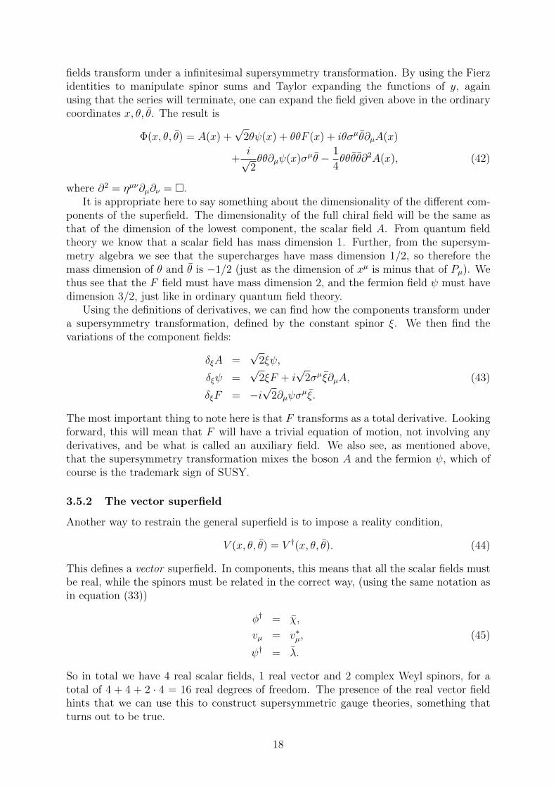
fields transform under a infinitesimal supersymmetry transformation. By using the Fierzidentities to manipulate spinor sums and Taylor expanding the functions of y, againusing that the series will terminate, one can expand the field given above in the ordinarycoordinates x, θ, θ. The result is

Φ(x, θ, θ) = A(x) +√

2θψ(x) + θθF (x) + iθσµθ∂µA(x)

+i√2θθ∂µψ(x)σµθ − 1

4θθθθ∂2A(x), (42)

where ∂2 = ηµν∂µ∂ν = .It is appropriate here to say something about the dimensionality of the different com-

ponents of the superfield. The dimensionality of the full chiral field will be the same asthat of the dimension of the lowest component, the scalar field A. From quantum fieldtheory we know that a scalar field has mass dimension 1. Further, from the supersym-metry algebra we see that the supercharges have mass dimension 1/2, so therefore themass dimension of θ and θ is −1/2 (just as the dimension of xµ is minus that of Pµ). Wethus see that the F field must have mass dimension 2, and the fermion field ψ must havedimension 3/2, just like in ordinary quantum field theory.

Using the definitions of derivatives, we can find how the components transform undera supersymmetry transformation, defined by the constant spinor ξ. We then find thevariations of the component fields:

δξA =√

2ξψ,

δξψ =√

2ξF + i√

2σµξ∂µA, (43)

δξF = −i√

2∂µψσµξ.

The most important thing to note here is that F transforms as a total derivative. Lookingforward, this will mean that F will have a trivial equation of motion, not involving anyderivatives, and be what is called an auxiliary field. We also see, as mentioned above,that the supersymmetry transformation mixes the boson A and the fermion ψ, which ofcourse is the trademark sign of SUSY.

3.5.2 The vector superfield

Another way to restrain the general superfield is to impose a reality condition,

V (x, θ, θ) = V †(x, θ, θ). (44)

This defines a vector superfield. In components, this means that all the scalar fields mustbe real, while the spinors must be related in the correct way, (using the same notation asin equation (33))

φ† = χ,

vµ = v∗µ, (45)

ψ† = λ.

So in total we have 4 real scalar fields, 1 real vector and 2 complex Weyl spinors, for atotal of 4 + 4 + 2 · 4 = 16 real degrees of freedom. The presence of the real vector fieldhints that we can use this to construct supersymmetric gauge theories, something thatturns out to be true.

18

A thing to note is that if Φ is a chiral superfield, the real part of Φ, or equivalentlyΦ + Φ†, will be a vector superfield. The vector component of this field will be a derivativeof a scalar field. This suggests that we can define a superfield analogue to the U(1) gaugetransformation of the vector potential of electrodynamics, i.e. if V is a vector superfieldwe can make the transformation

V 7→ V + (Φ + Φ†), (46)

which will transform the vector component of V as

vµ 7→ vµ + i∂µ(Φ + Φ†),

which is just as the case of an ordinary U(1) transform of a vector potential. By workingout how the different components are affected by the gauge transform, one can find thatthe combinations

λα = ψα −i

2(σµ)αβ∂µφ

β

D = d− 1

2∂2f (47)

are gauge invariant under the transformation in eq. (46).2 Further, if one looks at howthe other component fields transforms, one can see that a gauge can be chosen such thatit eliminates most of them, which can simplify calculations a lot. In this gauge, known asthe Wess-Zumino gauge, the vector field becomes

V = θσµθvµ + (θθ)θλ+ (θθ)θλ+ (θθ)(θθ)D. (48)

From this we see that the actual, physical degrees of freedom, those that can not betransformed away by a gauge transformation, are those of a real vector, one (complex)Weyl spinor and one real scalar field. A thing to note is that the number of bosonic andfermionic freedoms doesn’t match. This is because the choice of gauge breaks supersym-metry. In fact, as we will see when constructing the abelian gauge theory Lagrangian, theD field will turn out to be unphysical.

We could now check how the components of the vector field transforms under a super-symmetry transformation, but we restrict ourselves to the case of the D field. By usingthe representations of the supercharges as differential operators on superspace we find

δξD = ∂µ(ξσµλ(x) + λ(x)σµξ). (49)

Just as for the F field in the chiral superfield, we see that the D field changes by a totalderivative, a fact that is crucial to constructing a supersymmetric Lagrangian involvingvector fields. This is really the next step in this review, but first we introduce someadditional notation that is useful for writing down supersymmetric actions.

3.6 Superspace integrals

In order to later write down supersymmetric actions in terms of superfields, we introducethe concept of integrals over superspace. These are not integrals in a proper sense, there

2 The naming of the D field coincides with the supercovariant derivative, but it will hopefully be clearfrom the context, and the name is used in all the literature so there is no sense in adopting a differentname.

19

is not really any valid integration measure, but they are rather formal definitions, intro-ducing convenient notational devices. The “usual” integral over Grassmann numbers iscalled the Berezin integral [16], and it is used, besides in supersymmetry, when we wantto quantize fermions using the path integral method. When you define it, you want topreserve some basic properties of ordinary integrals, i.e. that it should be insensitive toshifting the integral variable by a constant, in the sense that∫

f(x+ η)d(x+ η) =

∫f(x)dx,

where η is some constant, and it should be a linear operation. In order to keep these twoproperties we see that practically the only natural way to define it is∫

dξ(a+ bξ) = b. (50)

If we compare this with taking the derivative, we see that they are the same:∫dξ(a+ bξ) =

∂

∂ξ(a+ bξ) = b. (51)

This definition of the integral is easily generalized to integration over our superspaceGrassmann spinors. If we use the notation

d2θ = −1

4dθαdθβεαβ, d2θ = −1

4dθαdθβε

αβ (52)

d4θ = d2θd2θ (53)

we get that ∫d2θ(θθ) = 1,

∫d2θ(θθ) = 1,

∫d4θ(θθ)(θθ) = 1. (54)

What the integrals here do, which is what makes them useful, is that they extract com-ponents out of a function of θ and θ. For example, the integral of some function Φ(θ, θ)over d2θ2 really only picks out the θ2 component of Φ.

3.7 Supersymmetric Lagrangians

So far we have developed quite a bit of theory about abstract things like the supersymme-try algebra, superspace and superfields. In this section this formalism will be put to someuse and we will see how (relatively) easy these concepts make it to write down super-symmetric Lagrangians. By a supersymmetric Lagrangian we mean one that changes bya total derivative under supersymmetry transformations, so that the action is invariant.Without the concepts of superfields, it’s very hard to guess the form of the general super-symmetric action. We start by determining the simplest (sensible) Lagrangian involvinga single chiral superfield, and then we find the most general Lagrangian involving an arbi-trary number of chiral fields. Then we treat the supersymmetric extension of an abeliangauge theory, i.e. the supersymmetric version of QED. From here, one can continue totreat nonabelian gauge theories and talk about how renormalization works in supersym-metric theories and so on, but since this review was supposed to be brief, I will stop afterthat and in the next section instead introduce the simplest version of a supersymmetricextension of the standard model.

20

3.7.1 Lagrangians for chiral superfields

We first want a Lagrangian involving one chiral field Φ that is real, supersymmetric,Poincare invariant and of dimension 4 (so that the action is dimensionless). In fact thedimensionality and reality pretty much determine what the action must look like. Thedimension of the superfield is that of its lowest (in powers of θ) component, so as saidabove the chiral field will have mass dimension 1. We also know that the θ2 term, F ,has dimension 2, and remembering that the F component transforms as a total derivativeunder supersymmetry transformations (thus leaving the action invariant) we see that FF ∗

will be a real, globally supersymmetric action with the right mass dimension. Using theabove defined integral over superspace, we can write this action as∫

d4xd4θΦΦ† . (55)

This action is real, invariant under supersymmetry transformations, is Poincare invariantand has the correct dimension. By rewriting this in component form one can see that itdoes indeed contain the kinetic terms for the component fields A and ψ:

1

2∂µA∂

µA∗ − 1

4(A∂2A∗ + A∗∂2A) + FF ∗ − i

2(ξσµ∂µξ + ξσµ∂µξ) (56)

using some of the Fierz identities to simplify spinor expressions. We see here that the Ffield has no derivatives in the action, and therefore its equations of motion are trivial,

F = F ∗ = 0.

So we see that on shell, when the equations of motion hold, F is uniquely zero. F is whatis called an auxiliary field.

In order to add interactions to this theory, we note that the F field transforms as atotal derivative under supersymmetry transformations. This is in fact exactly what makesthe action above supersymmetric, but we see that another possibility is to take an actionthat just takes out the F component and make it real by adding the complex conjugate:∫

d4x

∫d2θm2Φ(x, θ) +

∫d2θm2Φ(x, θ)†

, (57)

where the m2 is there to give us the correct dimension. This also has all the desired prop-erties we want. And since the covariant derivative obeys the product rule of derivation,any analytic (or, as discussed above, holomorphic, for the word more often used in theliterature) function of a chiral field will again be a chiral field. This means that moregenerally the action ∫

d4x

∫d2θW (Φ) +

∫d2θW (Φ)†

(58)

where W is any analytic function of Φ (but not of Φ†), will be an acceptable supersym-metric action. This term adds mass and interaction terms to the Lagrangian, and W iscalled the superpotential. From dimensional grounds, we can see that W can be at mostcubic in the superfield. This follows since we know that in order to get a renormalizablepotential, all couplings must have non-negative dimension. The θ2 component of W (Φ)have mass dimension of one more than W itself, so if W is cubic in Φ this component willhave dimension 4 requiring the coupling to be dimensionless. Thus, W can be at mostcubic.

21

The general supersymmetric theory only involving one chiral field is called the Wess-Zumino model. Its action is∫

d4xd4θΦΦ† −∫

d4x

∫d2θ

(1

2mΦ2 +

1

3gΦ3

)+ h.c.

(59)

and it describes a massive complex scalar field and a massive fermion, with some interac-tion terms. Still, the F field has no derivatives acting on it in the action, so its equationsof motions will be trivial (although not as simple as in the free field case). By using thesolution of F :s equations of motions, we can eliminate F from the action. We note thatthe bosonic part of the Lagrangian is

LB = ∂µA∗∂µA+ F ∗F − (mAF + gA2F + h.c), (60)

so the equations of motion for F and F ∗ are

0 =∂LB∂F

= F ∗ −mA− gA2, (61)

0 =∂LB∂F ∗

= F −mA∗ − g(A∗)2. (62)

(63)

Using these, we can write the bosonic part of the action as

LB = ∂µA∗∂µA+ FF ∗ − (mAF + gA2F + h.c)

= ∂µA∗∂µA+ (mA− gA2)(mA∗ − g(A∗)2)

−((mA(mA∗ + g(A∗)2) + gA2(mA∗ + g(A∗)2)) + h.c.

)= ∂µA

∗∂µA− (mA− gA2)(mA∗ − g(A∗)2) = ∂µA∂µA− |F |2. (64)

So we see that the potential of the bosonic part of our Lagrangian, called VF is givensimply by VF (A,A∗) = |F |2. This also holds when we have a general superpotential,W (Φ). Then the scalar potential is given by the absolute square of the F -component, i.e.

VF (A,A∗) = |F |2 =dW

dΦ

∣∣∣∣Φ=A

. (65)

In this way, for a general supersymmetric potential, we can get part of our scalar poten-tial. However, as will be described towards the end of next section, when we add gaugeinteractions these also contribute to the scalar potential in a rather similar way.

3.7.2 Supersymmetric, abelian gauge theory

When we looked at the vector superfield, we defined the Wess-Zumino gauge in whichthe vector field only had 3 components. However, this gauge is not preserved by super-symmetry transformations, which is disappointing since it means that the vector field Vnecessarily has a lot of components. We can however define another vector field that onlycontains the three components, which will then be used write down our field strengthterm in our gauge theory Lagrangian. We begin with defining the chiral and antichiralfields

Wα = −1

4D2DαV, Wα = −1

4D2DαV (66)

22

where all the D’s are covariant derivatives and V is a vectorfield. Wα will obviously bechiral since

DβWα = −1

4DβD

2DαV = 0,

using that since Dα anticommutes and only has two components, D3 = 0. In the sameway, Wα is an antichiral field. One can show that Wα and Wα both are invariant underthe abelian gauge transformation (46), so there is no loss of generality in computing theircomponents in the aforementioned Wess-Zumino gauge. Using this gauge and writing Wα

as a function of the ‘chiral’ coordinate yµ = xµ + iθσµθ introduced above, one finds that

Wα(y, θ) = −iλα(y) + θαD(y)− i

2σµσνθαfµν(y) + (θθ)σµ

αβ∂µλ

β(y) (67)

where fµν = ∂µvν − ∂νvµ, D is a real valued scalar field and λ is a left handed spinor.fµν is, as can be suspected from its appearance, the ordinary field strength of our abeliangauge theory. The λ spinor has 4 real degrees of freedom, the D field has 1 real degree offreedom, and since the vµ has 4 degrees of freedom, where 1 can be eliminated by a gaugetransform, fµν which is gauge invariant must have 3 degrees of freedom, for a total of4 + 1 + 3 = 8 real degrees of freedom. This multiplet is called the field strength multipletand is an off-shell irreducible representation of the super-Poincare algebra.

So, since Wα is chiral, so is WαWα which in addition will be Poincare invariant. Thechirality means that the θ2 component will transform as a total derivative, and thus wecan use its real part as a valid supersymmetric Lagrangian,∫

dθ2WαWα +

∫dθ2W αWα. (68)

If you work this out in components, you find that this is

(λσµ∂µλ− λσµ∂µλ)− 1

2fµνfµν +D2. (69)

Just as for the F component in the chiral Lagrangian, there are no derivatives acting onthe D field. Thus it is another auxiliary field, with an equation of motion that is simplyD = 0. This Lagrangian then describes the free propagation of one gauge boson (throughthe fµνf

µν term) and its supersymmetric partner λ, called the gaugino.Only having a free gauge boson and gaugino isn’t very realistic or interesting, so the

natural next step is to ask how we can add charged matter fields to the theory. Forsimplicity, start with a single chiral field Φ taking values in a one dimensional represen-tation of the U(1) gauge group of our theory. That is, under a (global) gauge transform,exp(iφ) ∈ U(1), Φ transforms as

Φ 7→ eieφΦ, (70)

e being the charge of Φ. Then clearly the term Φ†Φ is gauge invariant (since Φ† 7→ e−ieφΦ†

under the same gauge transform). However, if we want to make the symmetry local andthus let φ → φ(x) be a function on spacetime, it is no longer guaranteed that eieφ(x)Φstill is a chiral superfield (since the covariant derivative in the definition of a chiral fieldinvolves ∂µ). So, we are in the uncomfortable situation that our local gauge transformviolates supersymmetry. In order to escape this predicament, we can let φ(x) be, insteadof a real valued function on spacetime, a full chiral field. Then eieφΦ will still be a chiralfield, and instead the Φ†Φ term will transform like

Φ†Φ 7→ eie(φ−φ)Φ†Φ. (71)

23

Now looking back at equation 46, we see that (φ − φ) can be absorbed into a gaugetransform of our vectorfield V . This suggests that a suitable, gauge invariant couplingbetween Φ and V is of the form Φ†eieV Φ, which indeed gives us back the correct couplingbetween a charged scalar field and a U(1) gauge field. So the Lagrangian looks like∫

d4θΦ†eieV Φ +

∫d2θ

1

4WαW

α + h.c.

. (72)

We note here that this scalar chiral field has no mass, since gauge invariance forbidsterms such as m2ΦΦ. If we want massive chiral fields, we can instead take two differentchiral fields Φ+ and Φ− with opposite charge, which allows us to add a gauge invariantmass term m2Φ+Φ− to the superpotential. So the full Lagrangian of what basically is thesupersymmetric extension of scalar quantum electrodynamics looks like∫

d4θ(Φ†+eieV Φ+ + Φ†−e

ieV Φ−) +

∫d2θ

1

4WαW

α +m2Φ+Φ− + h.c.

. (73)

If we look at the scalar potential of this Lagrangian, we find that in addition to the VFterm, that is the same as in the Wess-Zumino model, we also find a new term, comingmuch in the same way from the new auxiliary D component. This addition to the potentialnow looks like

VD =1

2g2D2 (74)

where D of course is rewritten using its equation of motion in terms of the other scalarfields in the theory. The full scalar potential thus is the sum V = VF + VD, somethingthat will be used later when we look at the potential for the Higgs fields. This is indeeda general theme, the scalar potential of any supersymmetric theory is the sum of thesquares of the auxiliary fields.

The simple abelian case can without too much trouble be generalized to the nonabeliancase of Yang-Mills theory, but in order to keep this review brief, this won’t be done here.The interested reader is invited to consult the vast literature, for example those reviewsmentioned in the beginning of this section, for this and much more interesting theoryabout supersymmetry.

3.8 Concluding remarks

Supersymmetry is a vast field with many remarkable results, and this brief review hasbut scratched at the very surface. The approach followed here, using superspace andsuperfields, can be extended into a full fledged approach to quantum field theory, withFeynman rules and so on. By doing this, people have been able to prove many remarkablenon-renormalisation theorems[17, 18]. Most important is the fact that supersymmetrictheories have no quadratic divergences. This basically comes from the pairing of bosonswith fermions, and since fermion masses only can be logarithmically divergent in a renor-malizable theory and supersymmetry requires the boson mass to be equal to the fermionmass there can be no quadratic divergences. In fact, there is no renormalization of anyof the parameters in the superpotential (i.e. masses and Yukawa couplings) apart from aglobal rescaling of the superfields. Gauge couplings are renormalized, however. If you goto theories with more supercharges, N > 1, even more divergences will disappear, and forN = 4 there will be no divergences at all. But as stated in section 3.2, N > 1 cannot bedirectly used to extend the standard model, which is what I next turn to.

24

4 Realistic supersymmetric models

In this section I will introduce the simplest way to extend the standard model into asupersymmetric theory, the minimal supersymmetric standard model (MSSM). Then anextension to this theory is presented, the next-to MSSM (NMSSM), mostly in orderto solve a problem concerning the value of a dimensionfull parameter in the MSSM.Since nature obviously isn’t supersymmetric at low energies, we also need to study howsupersymmetry is broken. This is a large subject which I won’t cover in any detail, onlyintroduce the concept of how we can introduce so called softly breaking terms into theLagrangian of our models, as discussed in the next section.

4.1 Softly breaking terms

The most popular ideas about how supersymmetry breaking works, is that it is sponta-neously broken, in a manner similar to how the gauge symmetries are broken. In fact,supersymmetry is broken as soon as the vacuum gets a nonzero energy, as mentioned insection 3.2 . This fact means that the breaking of supersymmetry and the breaking ofgauge symmetries are closely connected subjects. There are different additional termsyou can introduce into your Lagrangian, such that you can give the fields in these terms anon-vanishing VEV, and thus give the vacuum a nonzero energy, breaking supersymmetry.For more details, see [20].

When constructing realistic models, we don’t really need to care about the detailsof exactly how this happens. Instead, we can introduce terms into our Lagrangian thatexplicitly breaks supersymmetry, but at the same time preserves renormalizability andare such that at high energy, above the supersymmetry breaking scale, they becomeirrelevant. Such terms are called softly breaking terms, and are essentially things likescalar mass terms, gaugino masses or cubic scalar terms with dimensionfull couplings.For our purposes, analysing the Higgs sector at leading order, we only care about thescalar mass terms. So when we have the supersymmetric Lagrangian, we can then addall such allowed terms, and view them as an effective description of how supersymmetryis broken.

4.2 The MSSM

Just as it sounds, the MSSM is the model you get when you try to minimally extendthe standard model to incorporate supersymmetry. Since none of the particles in thestandard model have the same quantum numbers (excluding mass), one cannot let anyof the known particles be each others superpartners. So instead we let every particle bea part of a corresponding superfield, and then put the superfields in the same SU(2)Ldoublets as in the SM. The same of course applies to the gauge fields, which now becomepart of gauge superfields.

The supersymmetric partners are sometimes called sparticles to distinguish them fromthe normal particles, and are given names by adding either an ‘s’ at the beginning orputting ‘-ino’ at the end. The superpartner to the electron is called selectron, the partnersof the quarks are called sqarks, the W-boson has the Wino and we also have the photino,the gluino and so on. In formulae, these superpartners are usually denoted by putting atilde on top of the symbol for the regular particle, so that for example the selectron isdenoted e and the photino γ.

25

As mentioned briefly above, we also have new particles called neutralinos, which aremixtures of the neutral superpartners of the Higgs bosons (which naturally are called thehiggsinos) and the neutral gauginos. In the MSSM there are four different neutralinos,and the lightest one is usually assumed to be the lightest supersymmetric particle. Inthe same way, the charged higgsinos and winos (W±) mix to form mass eigenstates withcharge ±1, called the charginos, of which there are two.

In a supersymmetric theory, only a Higgs with hypercharge Y = 1/2 can have thenecessary Yukawa coupling to give masses to the up-type quarks with charge +2/3, andonly a Higgs with hypercharge −1/2 can have the necessary couplings to give mass tothe down-type quarks. This is because the superpotential is holomorphic, so the Higgsdoublet giving mass to the up-type quarks cannot also give mass to the down-type quarkssince we are not allowed to use the complex conjugate. Thus we at least need two differentHiggs SU(2)L-doublets in order to give mass to all the massive particles. We will call theY = 1/2 doublet Hu, and the Y = −1/2 doublet Hd. Then the upper component of theY = 1/2 will have isospin T3 = +1/2 and therefore have electric charge +e. The lowercomponent will be electrically neutral, and in the same way the upper component of theY = −1/2 doublet will be neutral while the lower will have a negative electric charge. Sothe superdoublets look like

Hu =

(H+u

H0u

), Hd =

(H0d

H−d

)(75)

and the Higgs fields which gives masses to the fermions will be the corresponding scalarfields. We can then note that the Higgs superdoublet Hd has the same quantum numbersas left handed leptons (and sleptons). Therefore we can use it to give mass to the leptonsas well as the down-type quarks, so we don’t need another Higgs doublet for this purpose.There is another way to motivate the need of two different Higgs doublets which is basedon anomaly cancellations, but this isn’t logically needed.

The minimal superpotential involving these superfields which in a reasonable wayextends the standard model is

WMSSM =∑i,j

yiju uiHu · Qj − yijd diHd · Qj − yije eiHd · Lj + µHu · Hd (76)

where the “hatted” letters denote the superfield doublets or singlets corresponding to thenormal SU(2)L doublets/singlets in the standard model, and i, j are generation indices,i = 1, 2, 3. That is, for the first generation, Q1 = (u, d)T , L1 = (eL, νe)

T , e1 = eR, u1 = uand so on. The Higgs doublets are as described above, and the yij are the Yukawacouplings among generations. The products of SU(2)L doublets are given by

A ·B = εabAaBb

where εab is the fully antisymmetric symbol in two dimensions with ε12 = 1 and a, b areSU(2)L indices. In this superpotential the µ parameter has dimension mass and is whatgives mass to the Higgs fields, and it is this simple fact which motivates the introductionof the next-to minimal supersymmetric standard model (NMSSM).

From this superpotential and the ordinary gauge couplings of the standard model, wecan calculate the scalar potential, by calculating the F and D terms as described above.Doing this, and looking only at the Higgs sector of the potential, we find

VF = µ2(|Hu|2 + |Hd|2) (77)

26

and

VD =1

8g2(|Hu|2 − |Hd|2

)2+

1

2g2

2|H†u ·Hd|2. (78)

As described above, we can then add the soft supersymmetry breaking terms;

Vsoft = m2Hu|Hu|2 +m2

Hd|Hd|2 + (m2

3Hu ·Hd + h.c.) (79)

where the dimensionfull parameters m2Hu,m2

Hdand m2

3 clearly have to be of the order ofthe weak or supersymmetric breaking scale. The total scalar potential is then the sumof these three terms. By letting at least one of m2

Huand m2

Hdbe negative, Hu and Hd

acquires non-zero VEVs, breaking the symmetry.From requiring vacuum stability we get some relations between m2

Hu,m2

Hd,m2

3, theVEVs and µ; as described in more detail in the next section for the NMSSM. Usingthese, one can calculate and then diagonalize the mass matrices that describe the physicalmass eigenstates in terms of the parameters of the model. The formulae are only statedhere without much explanation, mostly for some completeness and comparison with theNMSSM. Hopefully, how the calculations are done will become clear after reading thenext section as well as section 5, where the calculations leading to the mass matrices andmass eigenstates are explained in more detail.

In the MSSM, it turns out that we get one physical charged Higgs state, H±, with amass

m2H± =

(2m2

3

vuvd+

1

4g2

2

)v2

2(80)

where 〈H0u〉 = vu/

√2 and 〈Hd〉 = vd/

√2, i.e. the VEVs, and v2 = v2

u + v2d, which cor-

responds to the VEV of the Higgs in the standard model. We also get one neutral,pseudoscalar (CP-odd) Higgs, called A, with a mass

m2A =

2m23

sin 2β, (81)

where the useful angle β is defined from tan β = vuvd

. Finally, we also get two neutral

scalar (CP-even) Higgses, H1 and H2 (where H1 is lighter than H2), that have the masses

m2H1,H2

=1

2

[m2A +M2

Z ∓√

(m2A +M2

Z)2 − 4M2Zm

2A cos2 2β

]. (82)

If we remember the relation M2W = 1

4(v2/2)g2

23, and express sin 2β in terms of vu and vd,

we see thatm2H± = m2

A +M2W . (83)

We can also conclude thatm2H1

+m2H2

= m2A +M2

Z , (84)

and the more striking inequality

mH1 < min(mA,MZ), (85)

meaning that no matter how we choose our parameters, mH1 < MZ . This is a tree levelprediction, and loop corrections can lift the mass of H1 above the so far established limits,but this is still an important prediction of MSSM.

3The extra factor 1/2 coming from the factors of√

2 in my definition of vu and vd.

27

As we are excluding larger and larger values of mH1 , this is really a problem, calledthe little hierarchy problem. Just as the general hierarchy problem, this concerns theseparation of mass scales, because in order to generate the large loop corrections neededto increase mH1 , the other sparticle masses needs to become very large, again creatinga new unexplained mass scale in the theory. The maximal bound one can get withoutadding new dynamics to the theory is something like mH1 . 135 GeV. Thus results thatexclude a Higgs mass lighter than that will exclude the whole of MSSM.

As mentioned above, the µ and m23 parameters are dimensionfull. The m2

3 parameterisn’t a problem since it enters as one of the softly breaking terms, but µ enters throughthe ordinary Lagrangian, so the only natural values for it before SUSY breaking occurs,is either 0 or the Planck mass MP . However, to be phenomenologically viable we musthave a µ that is of similar size to the electroweak scale. Otherwise there would have to bemiraculous cancellations between µ2 and the soft supersymmetry breaking terms whichI have not yet introduced. It is in order to solve this problem we motivate the study ofthe NMSSM, where by adding a singlet Higgs field and coupling it to the Higgs doublets,the µ parameter is generated through supersymmetry breaking. This breaking gives thesinglet and the two Higgs doublets VEVs, and thus the singlet-doublet-doublet couplinggives us an effective µ. This explains why µ should be roughly the same scale as theelectroweak breaking scale.

For a more complete discussion of MSSM, and some discussion about how it may bediscovered, see for example [21].

4.2.1 R-parity

The superpotential described above is as stated the minimal one reproducing the resultsof the standard model. However, it is not the most general renormalizable superpotentialwe can write down; we could also include terms such as

λijkLi · Lj ek + ωijkQi ·Qj dk + κijkLi · Qj dk + νiLiHu

where again i, j, k are generation indices. However, all these terms enable decays orproduction processes that violates the observed lepton and baryon number conservation,unless of course the couplings for some reason are very suppressed, which would be mostunnatural. We could try and impose baryon and lepton number conservation directly,but this would be a step back compared to in the standard model, where this happens“automatically” since in the SM there are no allowed renormalizable terms that violateeither baryon or lepton number conservation. Moreover, there are known non-perturbativeeffects that violates baryon and lepton number conservation[22], so they are probably notexact symmetries of nature. Of course, the simple observation that the universe we seetoday consists of only matter as opposed to equal parts matter and antimatter shows thatsuch processes must be allowed.

In order to get rid of such terms, one imposes a new symmetry, called R-parity orequivalently, but slightly different, matter parity, that doesn’t allow lepton or baryonnumber conservation. In addition, it has other nice consequences, discussed shortly below.Matter parity assigns to each particle in the theory a number

PM = (−1)3(B−L) (86)

where B is the baryon number (quarks have B = 13) and L is the lepton number. Gauge

bosons carry neither number and so are assigned PM = 1. It is easy to check that both

28

the leptons and the quarks doublets have PM = −1 and the Higgs, carrying none of thenumbers has PM = 1 just as the gauge bosons. Matter parity is then to be a conservedquantum number, and the condition to be imposed is that we only allow terms with acombined (i.e. the terms matter parity multiplied together) parity of +1. This forbids allthe terms listed above.

An equivalent way of stating the symmetry that often is more useful is in terms ofR-parity, defined instead for every particle as

PR = (−1)3(B−L)+2s (87)

where s is the spin of the particle. As opposed to the matter parity, all particles in thesame supermultiplet do not have the same R-parity, since they differ by (in N = 1 SUSY)half a unit in spin. It is simple to check that this means that all the normal particles hasPR = +1, while the sparticles (i.e. superpartners) have PR = −1. Now the equivalentrequirement is instead that all interaction terms should preserve PR.

In the literature, one often encounters symmetries called “R-symmetries”, which arethings like additional U(1) symmetries you add to your model. These are not the same asR-parity, which is a discrete Z2 symmetry. Symmetries are called R symmetries when theydo not commute with supersymmetry. We can easily see that this is the case with R-parity,since it depends on the spin and the supercharges change the spin by 1/2 unit. However,since R-parity is equivalent with matter parity, which does commute with supersymmetry,there really is nothing truly “R” about R-parity.

If R-parity is conserved, as we impose it to be in MSSM and NMSSM, this has anumber of important consequences. It means that there can be no interactions with anodd number of sparticles, and that there can be no mixing between ordinary particlesand sparticles. In particular, this means that supersymmetric particles has to be pairproduced when we perform accelerator experiments with normal particles. It also meansthat the lightest supersymmetric particle (LSP) has to be stable, since there is no alloweddecay process to only normal particles. This is how supersymmetry provides a possibleexplanation for the cold dark matter in the universe. So the imposing of R-parity seems tobe well motivated from a phenomenological viewpoint. From a theoretical viewpoint, thereare numerous proposed extensions[23] of MSSM where R-parity appears as a remnant ofa continuous R-symmetry broken at some high energy scale.

4.3 The NMSSM

As stated above, the NMSSM [24, 25] is a proposed extension of the MSSM, which in anatural way solves the µ-problem. In order to get rid of the dimensionfull µ parameter, weadd a new Higgs SU(2)L singlet S to the theory. Of course, in principle nothing forbidsa µ term just because we add a new singlet, but we take it to have the “natural” value 0.The new superpotential looks like

WNMSSM = WMSSM + λSHu · Hd +1

3κS3, (88)

where λ, κ are new, dimensionless parameters of the model. From this superpotentialand the usual gauge couplings, the F and D part of the potential can be computed asdescribed in section 3.7. The result looks very much like in MSSM, but with some extraterms;

VF = |λS|2(|Hu|2 + |Hd|2) + |λHu ·Hd + κS2|2 (89)

29

VD =1

8g2(|Hu|2 − |Hd|2)2 +

1

2g2

2|H†u ·Hd|2 (90)

Since supersymmetry has to be broken, and we don’t know nor care about the details ofthe breaking mechanism, we also have to add to the potential all possible terms whichbreaks supersymmetry in the acceptable, soft way explained in section 4.1. This softpotential looks like

Vsoft = m2Hu|Hu|2 +m2

Hd|Hd|2 +m2

S|S|2 +

(λAλSHu ·Hd +

1

3κAκS

3 + h.c.

). (91)

Nothing is preventing us from adding the m23Hu · Hd term present in the MSSM case,

but this would add an additional parameter with mass dimension, in conflict with thephilosophy behind NMSSM, so we consider only the case m2

3 = 0. The entire Higgspotential is then given by the sum of these,

VHiggs = VF + VD + Vsoft. (92)

Then, as in the breaking of electroweak symmetry, we assume that m2S <

19κ2A2

κ so that

S = 0 is an unstable state. If we define 〈S〉 = vs/√

2 we see that when we expand thesinglet field around its VEV we get a term µ = λvs/

√2 with mass dimension4. Since this

term comes from supersymmetry breaking, it’s natural for it to have a value of magnitude|µ| . MSUSY, where MSUSY is the scale where supersymmetry is broken. This is the wayin which NMSSM solves the µ-problem of MSSM.

Further, we also assume that at least one of the other Higgs mass parameters m2Hu

and m2Hd

are negative, so that Hu, Hd also get nonzero VEVs, as required to break theelectroweak symmetry. We then have the gauge freedom to choose 〈H+

u 〉 = 〈H−d 〉 = 0, sothat the vacuum is uncharged. In this treatment, I will discuss the vacuum obtained byfurther assuming all the remaining VEVs to be real, and described by

〈Hu〉 =1√2

(0vu

), Hd =

1√2

(vd0

), 〈S〉 =

1√2vs. (93)

We then require this vacuum to be a stable local minimum of the potential, giving usthree different relations of the type

∂V

∂S

∣∣∣∣vacuum

= 0

relating the squared masses of the Higgs fields to the VEVs and the other parameters inthe theory. The derivatives w.r.t. fields with zero VEVs are trivially zero. If solved forthe masses, these three relations are

m2u ≡ m2

Hu+ |µ|2 =

1

8g2(v2

d − v2u) + λ

vsvd2vu

(√2Aλ + vsκ

)− 1

2λ2(v2

d + v2s) (94)

m2d ≡ m2

Hd+ |µ|2 =

1

8g2(v2

u − v2d) + λ

vsvu2vd

(√2Aλ + vsκ

)− 1

2λ2(v2

u + v2s) (95)

m2S = −1

2v2λ2 − v2

sκ2 +

1√2Aλλ

vuvdvs

+ vuvdκλ−1√2Aκvsκ. (96)

4Note that this definition of µ is a convention, which differs by a factor 1√2

from the most commonone.

30

These new masses (mu,md) are defined since when we give the singlet a VEV, effectivelythere will be an additional massterm of |µ|2 for the doublet fields, so we calculate the con-ditions for these effective masses. As above we define v =

√v2u + v2

d. These requirementsfixes the mass parameters. In order to further reduce the number of parameters, we can,as is usual, fix

v2 h (√

2 · 174 GeV)2 h (246 GeV)2,

where the factor of√

2 comes from my definition of vu and vd. This just sets the scale ofthe symmetry breaking to be the electroweak one. As said above when discussing MSSM,v corresponds to the Higgs VEV in the standard model, and the numerical value of 174GeV comes from the standard model relation

M2W =

1

4v2g2

2.

Just as in the MSSM above, it is useful to define an angle β from

tan β =vuvd.

We now see that a full specification of the Higgs sector in the NMSSM requires sixparameters:λ, κ,Aλ, Aκ, tan β and vs. Conventions can be chosen such that λ, tan β andvs are positive, and this is what I will do. For my purposes I also keep κ > 0, sinceswitching this sign doesn’t change any of my results. In my numerical studies I willreplace Aλ by the physical mass of the charged Higgs, mH± , which of course must bepositive, and we will see that the requirement of positive masses squared restrics Aκ tothe negative range.

The “MSSM limit” can be approached smoothly by keeping the ratio k = κ/λ fix andletting λ → 0, while keeping µ = vsλ/

√2 constant. Since the only couplings between

the Higgs doublets and the new Higgs singlet are dependent on λ and κ, the singlet fielddecouples in this limit and one recovers the Higgs sector of MSSM. How this works willbe explained in more detail in section 6.2.

Another thing worth mentioning about the NMSSM, is that it can be used to solve thelittle hierarchy problem of the MSSM. This is because if we let λ (or vs) become larger,the mass of the lightest Higgs gets larger, so by having a large λ we can get a large Higgsmass. This approach is sometimes called λ-SUSY[26]. In this approach we however giveup the requirement of perturbativity up to the GUT-scale.

5 Details of NMSSM

In this section I will go through some technical details about the Higgs sector of theNMSSM. First the mass matrices are described in some detail, and then the couplingsof the Higgs to the W/Z and the quarks are briefly described, introducing the conceptof reduced couplings in order to easily compare it with the standard model Higgs andthe MSSM. Finally some theoretical and experimental limits on the parameter space arediscussed. Some other articles discussing the Higgs sector of the NMSSM are [27, 28].

5.1 The mass matrices

Since mixing only can occur between states with the same quantum numbers, we get threedifferent mass matrices, one for the charged Higgs states, one for the scalar or CP-even

31

neutral states, and one for the pseudoscalar or CP-odd states. Since they are obtained bytaking derivatives of the potential, they are all real and symmetric. This is at tree level,taking higher order corrections into account this is no longer the case. The realness alsomeans that, at tree level, there is no CP violation.

5.1.1 Neutral scalar states

In the natural basis Hu,R, Hd,R, SR where the subscript R denotes the real part of thecorresponding scalar field, we get the mass-squared matrix as follows

M2s,11 =

1

4g2v2

u +λvsvd2vu

(√

2Aλ + vsκ) (97)

M2s,22 =

1

4g2v2

d +λvsvu2vd

(√

2Aλ + vsκ) (98)

M2s,33 = vsκ

(1√2Aκ + 2vsκ

)+

1√2λAλ

vdvuvs

(99)

M2s,12 = vdvu(λ

2 − 1

4g2)− 1

2vsλ(√

2Aλ + vsκ) (100)

M2s,13 = λ

(vs(vuλ− vdκ)− 1√

2Aλvd

)(101)

M2s,23 = λ

(vs(vdλ− vuκ)− 1√

2Aλvu

)(102)

where I’ve used the stability conditions to eliminate the mass parameters from the poten-tial in favour of the vacuum expectation values and couplings. This matrix doesn’t reallylend itself to much further algebraic simplification, so it is evaluated in the form givenhere and numerical methods are used to find it’s eigenvalues, which corresponds to thephysical masses of the CP-even Higgs states, which are denoted H1, H2, H3, ordered fromthe lowest mass to the highest.

5.1.2 CP-odd neutral states

In the natural basis H0u,I , H

0d,I , SI we get the following mass matrix for the pseudo-scalar

states:

M2p,11 =

1

2

vdvuvsλ(√

2Aλ + vsκ) (103)

M2p,22 =

1

2λvs

vuvd

(√

2Aλ + vsκ) (104)

M2p,33 = − 3√

2Aκvsκ+

vdvuvs

λ

(1√2Aλ + 2vsκ

)(105)

M2p,12 =

1

2λvs(√

2Aλ + vsκ) (106)

M2p,13 =

1

2vdλ(√

2Aλ − 2vsκ) (107)

M2p,23 =

1

2vuλ(√

2Aλ − 2vsκ) (108)

If the first two basis-elements are rotated with the angle β, a massless Goldstone modedecouples, and the new mass matrix (dropping the massless mode) in the basis (P1, P2)

32

becomes

M2p′,11 =

v2

2vuvdvsλ(√

2Aλ + vsκ) ≡M2A (109)

M2p′,22 =

vuvdvs

(1√2Aλ + 2vsκ

)− 3√

2Aκvsκ (110)

M2p′,12 = vλ(Aλ − 2κvs) (111)

where we introduce the mass parameter M2A. Note that this is not a physical mass, only

a parameter which can be taken as one of the parameters instead of Aλ. It can be useful,because in the MSSM-limit, MA becomes the physical mass of the pseudoscalar Higgs.The matrix that diagonalises this is of course a 2× 2 orthogonal matrix, and can thus beparametrized by an angle θA. The new basis in which the mass matrix is diagonal is then(

A1

A2

)=

(cos θA sin θA− sin θA cos θA

)(P1

P2

). (112)

5.1.3 Charged states

In the natural basis H+u,R, H

−d,R, the mass matrix for the charged states looks like

M2c,11 =

1

4v2d(g

22 − 2λ2) +

vdvsλ

2vu

(√2Aλ + κvs

)(113)

M2c,12 =

1

4vdvu(g

22 − 2λ2) +

1

2λvs(√

2Aλ + vsκ) (114)

M2c,22 =

1

4v2u(g

22/2− 2λ2) +

vsvuλ

2vd(√

2Aλ + vsκ). (115)

By a rotation through the mixing angle β, this gives a mass matrix in a new basisH±, G± with the only nonzero element

M2c′,11 =

v2

2vuvdvsλ(√

2Aλ + vsκ) +1

4g2

2v2 − 1

2λ2v2

= M2A +M2

W −1

2λ2v2 (116)

To get the second equality, we use the definition of M2A in addition to the previously noted

relation (g2v/2)2 = M2W . The state G± is a massless Goldstone mode. The charged Higgs

state is denoted by H±.

5.2 Reduced couplings

If we want to express how the physical Higgs particles, i.e. the mass eigenstates, coupleto fermions and gauge bosons, what one needs to do is to express the original weakeigenstates Hu, Hd, S in terms of the mass eigenstates H±, A1, A2, H1, H2, H3. This is ofcourse done by looking at the matrices that rotates the weak eigenstates into the masseigenstates, i.e. the mixing matrices as defined above.

We are primarily interested in how the V -boson couples to the different Higgses, whereV can be either W± or Z, and the couplings to quarks, since in the generic Higgs decay

H → ff , there is a factorm2

f

m2W

meaning that the heaviest fermion allowed dominates, i.e.

either the top or bottom quark.

33

The way to find these couplings is to write down the relevant terms in the Lagrangian,which is originally in terms of the weak eigenstates, and then re-express it in terms of themass eigenstates Hi, H

± and Aj. The details can be found in [28].In order to simplify the notation and keep it from getting unneedingly cluttered, we

define so-called reduced couplings, where we take the full coupling and divide out theassociated SM coupling,

GV V Hi≡ gV V Hi

gSMV V H, GZAiHj

=gZAiHj

GSMZHH

=gZAiHj

g/2,

where g =√g2

1 + g22, g1 and g2 being the gauge couplings of the electroweak force. Here,

V can stand for either W or Z, the reduced coupling will be the same in either case. Thereduced coupling we will look the most at is the HiV V coupling, since this measueres howstandard model like the scalar Higgses are. If we let Si = (Hu,R, Hd,R, SR) be the scalarweak eigenstates, and Hi =

∑j SijSj, (i.e. Sij is the mixing matrix), then this reduced

coupling is defined as[27]GHiV V = sin βSi1 + cos βSi2. (117)

The HiH±W∓ coupling is similarly given by

GHiH±W∓ = cos βSi1 − sin βSi2. (118)

Since these reduced couplings comes directly from orthogonal mixing matrices, we mayconclude that they should fulfil certain sum rules. This is because of the sum rules thatelements of orthogonal matrices fulfil: the sum of the squares of one row (or column) isequal to one. For the reduced couplings, this means∑

i

G2ZZHi

= 1,∑i

G2HiH±W∓

= 1. (119)

In the same way, the reduced couplings of the Higgses to the top and bottom quarks alsocomes directly from an orthogonal matrix, but in this case a dependence on tan β alsoenters, since this describes how large the difference is between the two VEVs of the Higgsdoublets. In this case the sum rules are∑

i

G2Hitt

=1

sin2 β,∑i

G2Hibb

=1

cos2 β. (120)

We also have the sumrules from the columns, for example

G2HiV V

+G2HiH±W∓

+ S2i3 = 1, i = 1, 2, 3 (121)

where Si3 is the singlet component of Hi. If Si3 ≈ 0, then Hi will be purely doublet andthe corresponding sum rule G2

HiV V+ G2

HiH±W∓= 1 is recovered. Conversely, if Si3 ≈ 1

then both the other couplings will be suppressed, which means that detection of Hi willbe difficult. These sum rules are quite trivial in nature, but can be a useful check onthe numerical methods used. They are also important phenomenologically, since they ineffect is a good measure how standard model like the different Hi, Ai are. For example,in this last sum rule, if the first term is large it means that Hi is SM like, if the secondterm is large it means there’s a large coupling between the doublets making Hi MSSMlike, and the last term corresponds to how singlet-like Hi is.

Of course, since the standard model only has one (scalar) Higgs particle, only theH1 couplings (assuming that the lightest Higgs also will be the standard model like)have a direct correspondence in the standard model. Nevertheless we can define reducedcouplings by scaling away the gauge couplings and masses.

34

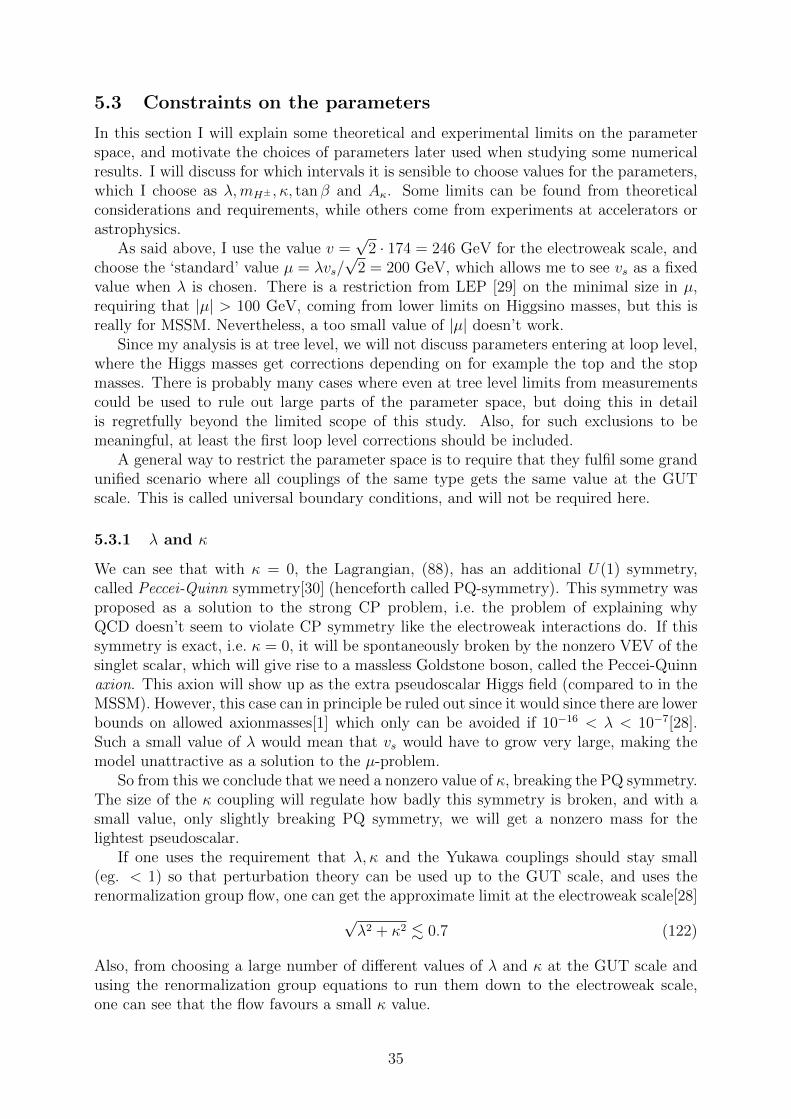
5.3 Constraints on the parameters

In this section I will explain some theoretical and experimental limits on the parameterspace, and motivate the choices of parameters later used when studying some numericalresults. I will discuss for which intervals it is sensible to choose values for the parameters,which I choose as λ,mH± , κ, tan β and Aκ. Some limits can be found from theoreticalconsiderations and requirements, while others come from experiments at accelerators orastrophysics.

As said above, I use the value v =√

2 · 174 = 246 GeV for the electroweak scale, andchoose the ‘standard’ value µ = λvs/

√2 = 200 GeV, which allows me to see vs as a fixed

value when λ is chosen. There is a restriction from LEP [29] on the minimal size in µ,requiring that |µ| > 100 GeV, coming from lower limits on Higgsino masses, but this isreally for MSSM. Nevertheless, a too small value of |µ| doesn’t work.

Since my analysis is at tree level, we will not discuss parameters entering at loop level,where the Higgs masses get corrections depending on for example the top and the stopmasses. There is probably many cases where even at tree level limits from measurementscould be used to rule out large parts of the parameter space, but doing this in detailis regretfully beyond the limited scope of this study. Also, for such exclusions to bemeaningful, at least the first loop level corrections should be included.

A general way to restrict the parameter space is to require that they fulfil some grandunified scenario where all couplings of the same type gets the same value at the GUTscale. This is called universal boundary conditions, and will not be required here.

5.3.1 λ and κ

We can see that with κ = 0, the Lagrangian, (88), has an additional U(1) symmetry,called Peccei-Quinn symmetry[30] (henceforth called PQ-symmetry). This symmetry wasproposed as a solution to the strong CP problem, i.e. the problem of explaining whyQCD doesn’t seem to violate CP symmetry like the electroweak interactions do. If thissymmetry is exact, i.e. κ = 0, it will be spontaneously broken by the nonzero VEV of thesinglet scalar, which will give rise to a massless Goldstone boson, called the Peccei-Quinnaxion. This axion will show up as the extra pseudoscalar Higgs field (compared to in theMSSM). However, this case can in principle be ruled out since it would since there are lowerbounds on allowed axionmasses[1] which only can be avoided if 10−16 < λ < 10−7[28].Such a small value of λ would mean that vs would have to grow very large, making themodel unattractive as a solution to the µ-problem.

So from this we conclude that we need a nonzero value of κ, breaking the PQ symmetry.The size of the κ coupling will regulate how badly this symmetry is broken, and with asmall value, only slightly breaking PQ symmetry, we will get a nonzero mass for thelightest pseudoscalar.

If one uses the requirement that λ, κ and the Yukawa couplings should stay small(eg. < 1) so that perturbation theory can be used up to the GUT scale, and uses therenormalization group flow, one can get the approximate limit at the electroweak scale[28]

√λ2 + κ2 . 0.7 (122)

Also, from choosing a large number of different values of λ and κ at the GUT scale andusing the renormalization group equations to run them down to the electroweak scale,one can see that the flow favours a small κ value.

35

0

100

200

300

400

500

600

700

800

-1000 -800 -600 -400 -200 0 200

Mas

ses

[GeV

]

A_kappa [GeV]

mH1mH2mH3mA1mA2

Figure 1: The masses as a function of Aκ, where tan β = 7,mH± = 250 GeV, κ = 0.3 andλ = 0.3.

We also note that if λ gets too small, this forces vs to become big, which means thatthe model no longer works well as a solution to the µ-problem. Even if we allow vs to takea value of a few TeV, say 2 TeV, which is well over but still “close” to the electroweakscale in some sense, this places a limit on λ & 0.1, so we get a rather stringent conditionon λ.

If universal boundary conditions at the GUT scale are imposed (which gives us the socalled constrained NMSSM[31]), we also get that the ratio λ/κ has to be close to 3. Thisis however not something that will be exclusively used since I don’t in general imposeuniversal boundary conditions.

5.3.2 tan β and Aκ

The range of Aκ is rather tightly constrained from the condition of vacuum stability. Infigure 1, the only allowed range of Aκ is where all the masses are positive, i.e. −600 .Aκ . −30 GeV. In many cases the limits are a lot stricter than this. From such plots youcan also see that for some choices of the other parameters there are no acceptable value ofAκ at all; in some cases the lightest pseudoscalar and the lightest scalar never both get apositive mass at the same time. For the coming plots where the Aκ dependence matters,the value of Aκ is chosen roughly in the middle of its allowed range, for a typical value ofthe running parameter. The typical values are −100 and −250 GeV.

As for tan β, an analysis of the running couplings shows that a low value of tan β isfavoured. However, experiments rule out a too small value, so a not so small value isrequired [27].

The theoretical upper bound is tan β . mt/mb ∼ 50, and I will briefly study whathappens when you take a large value, tan β = 30 in the model. See also [32] for a studyof what happens when you saturate this upper bound. We also have a lower boundtan β & 1.2 from requiring λt, the top quark Yukawa coupling, to remain small up to theGUT-scale.

36

5.3.3 mH± and the other Higgs masses

For the Higgs masses experiments have placed general lower limits. For the neutralHiggses, LEP has published negative search results[29] in some different decay channels,and depending on the precise branching ratios the limits looks a little bit different, butgenerally the lower bound from LEP is around mHi

> 80−90 GeV, for the MSSM. In theNMSSM these limits can be avoided, but they still give some kind of general guidelines.In the numerical studies, a lower value of mH± = 90 GeV, and a higher value of 250 GeVwill be used, when we don’t let mH± vary.

From different experiments at the Tevatron and LEP, rather strict limits can be placedon a SM-like Higgs[1], for example the Tevatron has excluded the range 158 GeV < mh <173 GeV, and from LEP we have exclusions of a mass lower than 114 GeV, but since thecouplings to fermions and gauge bosons of the MSSM or NMSSM Higgs bosons can besuppressed compared to the SM Higgs, these limits can be avoided.

6 Results

In this section I will present numerical results that explores some of the features ofNMSSMs parameter space. First, masses and couplings are treated as a function ofthe charged Higgs mass. From this we see some possibly interesting features of the model.Then it is studied how the masses and reduced couplings (and thus the mixing) behavein some different kinds of MSSM limits.

Since my calculation is only at tree level, it is not sensible to compare directly withexperimental limits. Even so, the general features are maybe even better understoodat tree level, since it is easier to compare directly with the formulae without too muchcluttering of the expressions. For my numerical results, I’ve written code in Java, usingthe basic linear algebra library Jama to diagonalize and find eigenvalues of matrices.

6.1 Varying the charged Higgs mass

In order to see how the NMSSM mass spectra behaves, it can be instructive to plot themasses as a function of the charged Higgs mass. From these plots, and the requirementof vacuum stability (i.e. m2

H1> 0, the lightest scalar mass positive) we can find limits on

allowed values for mH± for fixed values of the other parameters.As an aside, just in order to confirm the theory and my numeric calculation, we can

check that the sum rules for the reduced couplings actually holds in practise, which itturns out they do. A thing to note when looking at plots of reduced couplings and cos θAis that what I really plot is the absolute value of the couplings. This is for two reasons,first of all that all we really care about is the strength of the different couplings, the signcan of course matter (mostly when you go to higher orders) but not for our purposes here.The other reason is that the numerical method used switched signs discontinuously, sowithout taking the absolute value the graphs looks very discontinuous and strange. Thiscan probably be fixed rather easily, but since the sign doesn’t matter for our purpose noeffort was expended on this.

6.1.1 The NMSSM with a small κ

In figure 2 we can see that for the following choices of parameters, λ = 0.3, κ = 0.1,tan β = 2, Aκ = −100 GeV, mH± has to be between 360 and 550 GeV. This case is

37

0

100

200

300

400

500

600

700

800

900

1000

1100

0 100 200 300 400 500 600 700 800 900 1000

Mas

ses

[GeV

]

mH+ [GeV]

mH1mH2mH3mA1mA2

(a) Masses

0

0.2

0.4

0.6

0.8

1

0 100 200 300 400 500 600 700 800 900 1000

Red

uced

cou

plin

gs

mH+ [GeV]

H1VVH2VVH3VV

cosThetaA

(b) HiV V -couplings and cos θA

0

0.2

0.4

0.6

0.8

1

0 100 200 300 400 500 600 700 800 900 1000

Red

uced

cou

plin

gs

mH+ [GeV]

H1HpWH2HpWH3HpW

(c) HiH±W∓-couplings

0

0.2

0.4

0.6

0.8

1

0 100 200 300 400 500 600 700 800 900 1000

Red

uced

cou

plin

gs

mH+ [GeV]

S13S23S33

(d) Si3

Figure 2: The Higgs masses, some different scalar couplings and cos θA as functions ofmH± , for κ = 0.1, λ = 0.3, Aκ = −100 and tan β = 2. In (b,c,d), the physical range ofthe parameter space is inside the two black lines. Si3 is the singlet component of the Hi

state.

38

representative for a small κ-value, which corresponds to a slightly broken PQ-symmetry.This is favoured by the renormalisation group flow. From the figure we also see thatthe mass of the lightest pseudoscalar almost doesn’t change as soon as mH± gets above∼ 250 GeV. This is the singlet dominated pseudoscalar whose mass mainly comes fromthe 1

3κS3 term in the Lagrangian. The heavier states that grows more or less linearly are

the fields with little mixing with the singlet, (as seen from that S33 and cos θA both aresmall) and behave the same way as in the MSSM. For these parameters, the next lightestscalar state, mH2 also doesn’t depend very strongly on mH± , and grows much slower thanin MSSM.

So we see that even though the spectra of high mass states stay roughly the same,the three light Higgs states means that a NMSSM with parameters close to these willbe easily distinguished from MSSM, even if we only find the lighter Higgses. Of course,this only works if the reduced couplings, GHiV V and GA1HiZ doesn’t become too small toprevent detection, which happens in a small part of the relevant parameter space.

In figure 2.b the couplings of the scalar fields to the W/Z bosons as well as cos θAare plotted as a function of the charged Higgs mass. Since the reduced couplings can bethought of as a measure of the mixing between weak eigenstates, this plot shows that themixing depends on the charged Higgs mass in a slightly complicated way. The lightestHiggs is as one might guess the most standard model like, and it is the mixing with H2

which raises m2H1

above zero. For a specific value, mH± = 466 GeV, the coupling GH2V V =0, so if this specific scenario is true, the next-lightest Higgs would be totally singlet-like(as we see in figure 2.d). In this case, the H2 Higgs would be totally undetectable throughthe channels used to look for the standard model Higgs. We also see that in the physicalrange at least, the pseudoscalar mixing only varies a little. The HiH

±W∓ couplings,which measure how doublet or MSSM-like the scalars are, vary very little in the physicalrange, but we do see that H1H

±W∓ pass through zero when mH± = 449 GeV. We alsosee that the heavy H3 is doublet-dominated.

From the figure we can also see that mA1 and mA2 seems to switch behaviour withrespect to the charged Higgs mass around mH± ∼ 150 GeV. This switch is also apparentin how cos θA behaves. After this however, the pseudoscalar mixing stays more or lessconstant, and doesn’t vary rapidly in the physical region as the scalar mixing does. Inthe same way we see the switch in behaviour between mH2 and mH3 reflected in how allof the corresponding couplings switch, although this is outside the physical region.

6.1.2 Larger κ

If we let the value of κ get larger, the PQ symmetry is more badly broken and the lighterpseudoscalar gets a larger mass. This is not favoured by the renormalization group flow,but we have no a priori reason to exclude it. In figure 3 we have plotted the mass spectrumand couplings as functions of mH± for κ = 0.5. In this case, the lightest Higgs is the moststandard model like by far, and H2, H3 again switch behaviour, around mH± ' 520 GeV.

We also see that this large κ loosens the constraints on mH± from vacuum stability.The value of Aκ = −500 GeV used in the figure has been chosen approximately in themiddle of its allowed range for these parameters.

In this case, compared to the previous case with κ small, we see that apart fromthe lightest Higgs, the rest of the masses are significantly larger. However, they are notextremely heavy and are still very much within the range of detection, but the spectrumof light Higgses present in the previous case is absent. This would make it harder in this

39

0

200

400

600

800

1000

1200

0 100 200 300 400 500 600 700 800 900 1000

Mas

ses

[GeV

]

mH+ [GeV]

mH1mH2mH3mA1mA2

(a) Masses

0

0.2

0.4

0.6

0.8

1

0 100 200 300 400 500 600 700 800 900 1000

Red

uced

cou

plin

gs

mH+ [GeV]

H1VVH2VVH3VV

cosThetaA

(b) HiV V -couplings

0

0.2

0.4

0.6

0.8

1

0 100 200 300 400 500 600 700 800 900 1000

Red

uced

cou

plin

gs

mH+ [GeV]

H1HpWH2HpWH3HpW

(c) HiH±W∓-couplings

0

0.2

0.4

0.6

0.8

1

0 100 200 300 400 500 600 700 800 900 1000

Red

uced

cou

plin

gs

mH+ [GeV]

S13S23S33

(d) Si3

Figure 3: The Higgs masses, some of the scalar couplings and cos θA, as functions of mH± ,for κ = 0.5, λ = 0.3, Aκ = −500 and tan β = 2. In (b,c,d) the physical range is againbetween the black lines.

40

0

500

1000

1500

2000

2500

3000

0 500 1000 1500 2000 2500 3000

Mas

ses

[GeV

]

mH+ [GeV]

mH1mH2mH3mA1mA2

(a) Masses

0

0.2

0.4

0.6

0.8

1

0 500 1000 1500 2000 2500 3000

Red

uced

cou

plin

gs

mH+ [GeV]

H1VVH2VVH3VV

cosThetaA

(b) HiV V -couplings

Figure 4: The Higgs masses and reduced couplings of the scalar states to the Z and Wbosons, as functions of mH± , for a higher value of vs, equivalent to µ = 1000 GeV, insteadof the normally adopted value of µ = 200 GeV. The rest of the parameters are the sameas in figure 2. In (b), the physical range is inside the vertical black lines.

case to distinguish between the MSSM and the NMSSM if only the two lightest Higgsescan be detected, compared to the case with smaller κ.

Just as in the previous case, the pseudoscalar mixing, i.e. cos θA, stays rather constantexcept at the place where the two pseudoscalar fields switch identity. In this case thisswitching behaviour is more distinct, something we see both in how the masses and howcos θA behaves.

6.1.3 A larger vs or µ-value

If we vary the expectation value of the singlet field, vs, or equivalently the value of theeffective µ = vsλ parameter, this doesn’t change the qualitative behaviour of the massspectrum very much, but it changes the quantitative behaviour. All but the lightest Higgsgets heavier, including the charged Higgs, since the region of vacuum stability gets pushedupwards, see figure 4. We also see that the constraint from vacuum stability is relaxed(see for comparison figure 2), and that the charged Higgs mass, as well as the masses ofH3 and A2 are now forced to be larger than ∼ 1.5 TeV. Since the lightest of the Higgsesremains light, it means that a higher vs must make the H1 more SM-like, which meansthat the H2 becomes more singlet-like. That H1 becomes doublet-like means that itscoupling to W and Z should become large, and this is indeed also the case, as we can seein the right panel of figure 4.

If we make the same plots for a large value of κ, the effect on the mass spectrum willbe bigger and the heavy states will thus be even heavier, since it gets amplified by thelarge κ value. In this case the heavy singlet dominated fields will decouple and the lowermass states will behave like in the MSSM, so in this case the distinction between NMSSMand MSSM will be hard to find.

41

0

100

200

300

400

500

600

700

800

900

1000

0 100 200 300 400 500 600 700 800 900 1000

Mas

ses

[GeV

]

mH+ [GeV]

mH1mH2mH3mA1mA2

(a) Small couplings

0

100

200

300

400

500

600

700

800

900

1000

1100

0 100 200 300 400 500 600 700 800 900 1000

Mas

ses

[GeV

]

mH+ [GeV]

mH1mH2mH3mA1mA2

(b) Large couplings

Figure 5: The Higgs masses as a function of mH± for tan β = 35. In (a),we have κ =0.1, λ = 0.1, while in (b) κ = 0.5, λ = 0.5. In both cases Aκ = −100 GeV.

6.1.4 Large tan β values

What happens if you increase the value of tan β, making one of the doublet VEVs muchlarger than the other? In figure 5, this is shown as a function of the charged Higgs massfor two different choices of the singlet couplings. From the figure we see that there seemsto be rather distinct points where the identity of two different Higgses seem to switch.For example, the H1 and the H2 seem to switch behaviour with respect to the chargedHiggs mass at around mH± = 120 GeV. This kind of behaviour really comes from theway the mixing matrices depends on mH± (or equivalently Aλ) and from how we labelthe different states. A large tan β value means that the mixing with the Hu doublet willbe much more important in terms of mass than the mixing with the Hd doublet. Fromthis we can understand why a larger tan β value makes the identities of the Higgses moresharply defined.

What is perhaps more interesting to note is that we have three masses here that arealmost independent of the charged Higgs mass, even though exactly what we call the statevaries with mH± . This is also coupled to the fact that the couplings in this plot is rathersmall, κ = λ = 0.1. If we instead make them larger, we instead get the behaviour seenin figure 5, where the “switching” behaviour is not at all as sharp. Increasing the singletcouplings also pushes the lowest physically allowed value for mH± upwards (i.e. the valuewhere mH1 > 0), and seems to give the lightest scalar Higgs a very small mass.

6.2 The MSSM limit

A few things can be noted analytically when we take the limit λ, κ → 0 while keepingκ/λ = k fixed. For example, we can see that the parameter m2

s in the Lagrangian willapproach a fixed value as soon as λ and κ get small. This is seen by looking at theexpression for m2

s we got from the requirement of vacuum stability, equation (96). Sincewe keep µ = 1√

2vsλ fixed, we have that

m2s = −1

2v2λ2 − v2

sκ2 +

1√2Aλλ

vuvdvs

+ vuvdκλ−1√2Aκvsκ

42

= −1

2v2λ2 − 2µ2k2 +

1

2Aλλ

2vuvdµ

+ vuvdkλ2 − Aκkµ

→ kµ(Aκ − kµ) as λ→ 0,

also using the relation between κ and λ. If we instead keep κ fixed and let λ→ 0, we seethat instead

m2s = −1

2v2λ2 − v2

sκ2 +

1

2Aλλ

2vuvdµ

+ vuvdκλ− Aκκµ

λ→ ∞, as λ→ 0.

10

100

1000

10000

100000

1e+006

0.0001 0.001 0.01 0.1 1

Mas

ses

[GeV

]

lambda

mH1mH2mH3mA1mA2

Figure 6: How the masses vary when λ goes to zero while keeping κ fixed. In this plot,tan β = 2,mH± = 250 GeV, κ = 0.1 and Aκ = −100 GeV.

This behaviour is shown in figure 6, and it means that just as we can see from lookingat the Lagrangian (88), as λ goes to zero the singlet field decouples and the masses of thesinglet dominated states blow up.

Another way of taking an interesting limit is to let κ → 0 keeping λ constant, ascan be seen in figure 7. Here we see that in this limit (which really isn’t a proper MSSMlimit since λ stays large and thus the singlet doesn’t fully decouple), the A1 state becomesmassless, which again is because we restore the PQ symmetry turning A1 into the masslessPQ-axion. However, it is seen that for all cases with fixed λ there is no way of keepingH1 at a positive mass squared as κ goes to zero. For smaller values of λ, m2

H1becomes

negative for smaller values of κ, but any given value of λ ultimately restricts the lowestpossible value of κ. So from looking at this in addition to the above discussed λ → 0limit we see that in order to decouple the singlet and reduce the theory to MSSM, oneis in effect forced to take the simultaneous limit κ, λ → 0 (or in addition take the limitAκ → 0 as studied later).

In figure 8, we see that when approaching the MSSM limit in the sensible way, none ofthe masses becomes large, which is understandable since we above showed that m2

s tendstowards a finite value. However, also in this case the singlet decouples and does not mixwith the other fields, which we see by looking at the reduced couplings and cos θA, seeingthat the lightest Higgs state becomes completely standard model like, and also cos θA goesto 1, so that both mixing matrices become block diagonal and there is no mixing between

43

0

100

200

300

400

500

600

700

800

900

1000

0 0.1 0.2 0.3 0.4 0.5 0.6 0.7

Mas

ses

[GeV

]

kappa

mH1mH2mH3mA1mA2

Figure 7: The masses as a function of κ, where tan β = 7,mH± = 250 GeV, Aκ = −100GeV and λ = 0.3.

the doublet and the singlet. That the lightest scalar becomes standard model like in thislimit means that for small κ and λ of roughly the same size (k ∼ 1) means that it couldbe detected as easily as in the standard model.

We also see that cos θA goes to 1 much slower than the reduced scalar couplings. Thisis not a general feature but depends on the value of k. However, I’ve not found anycases with k > 1 where the pseudoscalar mixing disappears slower than the scalar mixing.This means that small values of λ and κ suppresses mixing between scalar singlet anddoublet states much more than between the pseudoscalar states. Moreover, as λ becomessmall the mixing between the scalar Higgs fields stop depending on λ and stays more orless constant. This is of course very reasonable since λ determines the coupling strengthbetween the singlet and the doublets.

However, as we can see in figure 9, the reduced couplings (and thus the mixing)doesn’t always vary slowly when we take the limit. This behaviour seems to occur onlywhen k . 0.5, in the figure we have k = 0.2 as a representative case. In these scenarios,the couplings continue to vary very rapidly (considering the logarithmic scale) even whenλ is very small, and the mixing only disappears when λ becomes really small. Differentlyfrom before, the lightest Higgs isn’t the most standard-model like in this scenario. Thisrole is instead filled by H2. We also note that the masses of H1 and H2 gets very similarin the MSSM limit.

Since cos θA approaches 0, we see that the lightest pseudoscalar state also decouplesin the MSSM limit (that cos θA = 0 of course means that the off-diagonal element of thepseudoscalar mixing matrix sin θA = 1).

We however see that the masses of the two lightest Higgses are very small for theseparameter choices, so this particular case is not realistic. For such small values of k therequirement that m2

H1> 0 seems to rule out most of the parameter space, i.e. for many

choices of other parameters, m2H1

< 0. I’ve not found any case where the same thinghappens for the pseudoscalar mixing, but no methodical search of such a scenario wascarried out.

As we can see from the formula for m2S in the MSSM limit, if we let the ratio k = κ/λ

get larger, then the masses of the singlet states should increase. And this is exactly

44

0

50

100

150

200

250

300

350

400

450

0.001 0.01 0.1 1

Mas

ses

[GeV

]

lambda

mH1mH2mH3mA1mA2

(a) Masses

0

0.2

0.4

0.6

0.8

1

1.2

0.01 0.1 1

Red

uced

cou

plin

gs

lambda

H1VVH2VVH3VV

cosThetaA

(b) HiV V -couplings and cos θA

Figure 8: The masses, HiV V -couplings and cos θA as the MSSM limit is approached,using k = 1, tan β = 2,mH± = 250 GeV and Aκ = −100.

0

50

100

150

200

250

300

0.001 0.01 0.1 1

Mas

ses

[GeV

]

lambda

mH1mH2mH3mA1mA2

(a) Masses

0

0.2

0.4

0.6

0.8

1

1.2

0.001 0.01 0.1 1

Red

uced

cou

plin

gs

lambda

H1VVH2VVH3VV

cosThetaA

(b) Couplings and cos θA

Figure 9: How the masses, cos θA and HiV V couplings vary when approaching the MSSMlimit, using k = 0.2, tan β = 2,mH± = 250 GeV and Aκ = −100 GeV.

what happens as we can see in figure 10, where a larger k value is seen to push theheaviest scalar, the singlet dominated one, far up in mass, whereas the mass of the heavypseudoscalar is also increased but not at all as much.

Another possible way of approaching the MSSM limit is to also send the Aκ parameterto zero, which effectively further suppress the S3 term in the Lagrangian and thus restoresthe PQ-symmetry. And as we can see in figure 11, in this case the lightest pseudoscalarHiggs become massless in the limit, restoring the massless PQ axion. In this limit, wealso see that the pseudoscalar mixing disappears (cos θA → 1) and that the lightest scalarHiggs again is fully standard model like.

One could also imagine letting vs go to zero smoothly, but in order to keep µ in anacceptable range this would mean that λ would have to become larger than allowed bythe requirement of perturbation theory being valid up to the GUT-scale, i.e. λ . 0.7 asstated before. A small value of µ is excluded from bounds on the chargino masses[1] from

45

0

100

200

300

400

500

0.001 0.01 0.1 1

Mas

ses

[GeV

]

lambda

mH1mH2mH3mA1mA2

(a) k = 2

0

500

1000

1500

2000

2500

3000

3500

4000

4500

0.001 0.01 0.1 1

Mas

ses

[GeV

]

lambda

mH1mH2mH3mA1mA2

(b) k = 10

Figure 10: How the masses vary when approaching the MSSM limit for two differentvalues of k. The rest of the parameters have the same value as those in figure 8.

direct searches. As said towards the end of section 4.3, we can give up the perturbativerequirement and consider λ 1 as in the λ-SUSY model [26], in which case this limitcould be viable.

7 Summary and conclusions

In this study, we have briefly reviewed the motivation behind studying supersymmetry,followed by a short introduction to the very basics of supersymmetry in the superspaceand superfields formulation. Then the MSSM was described, and its simplest extension,the NMSSM was introduced as a solution to the µ-problem. Some technical details ofthe Higgs sector of NMSSM was stated, including the mass matrices and definition of thereduced couplings. This was followed by some numerical studies of different choices ofparameters, including a look at approaching the MSSM limit in some different ways.

We find that in the by renormalization group flow favoured choice of κ, tan β andλ, the mass spectra with three different relatively light Higgs bosons should make thetheory easy to distinguish from the MSSM even when not all the Higgses are detected.But in other perfectly allowed cases, the distinction might not be directly obvious. Wealso see that for this case some of the couplings to SM-particles pass through 0, so thatit is possible that for example the H2 state can be hidden and not interact in a standardmodel like way at all.

For a larger κ value, i.e. a more strongly broken PQ-symmetry, we see that the cou-plings behave in a qualitatively different way. In this case the switching behaviour takesplace inside the physically sensible area, but the couplings of the H1 state doesn’t showany complicated dependence on mH± . Over the whole range, H1 is the essentially fullystandard model like.

If we want to study the limits where the singlet decouple, from looking at what happenswhen only one of κ or λ are sent to zero, we conclude that sensible limits exists only whenboth of them are decreased simultaneously. When we approach this MSSM limit, keepingthe ratio κ/λ constant, the mixing with the singlet field disappears. Mostly this decouplinghappens rather quickly, but in some cases, when κ/λ . 0.5, the mixing of the scalar states

46

-300

-200

-100

0

100

200

300

400

500

0.0001 0.001 0.01 0.1 1 10

Mas

ses

[GeV

]

lambda

mH1mH2mH3mA1mA2

Akappa

(a) Masses

0

0.2

0.4

0.6

0.8

1

1.2

0.0001 0.001 0.01 0.1 1

Red

uced

cou

plin

gs

lambda

H1VVH2VVH3VV

cosThetaA

(b) HiV V couplings and cos θA

Figure 11: How the masses, couplings and cos θA vary when λ goes to zero while keepingk = κ/λ fixed, in addition to also sending Aκ to zero. In this plot, k = 1, tan β =2,mH± = 250 GeV. Aκ begins on a value of −250 GeV, and is sent to zero in the samemanner as λ and κ (i.e. we keep the ratio κ/Aκ constant).

depends strongly on the nonzero λ. We also see that in this case, the lightest Higgs isno longer necessarily the most standard model like, that role being taken by H2. But forλ > 0, both H1 and H3 are slightly standard model like, so if this is the case (i.e. we havea small λ and a ratio as described), we could detect three relatively light Higgs bosonswith different masses. However, these cases seem to depend very much on the ratio κ/λhaving a specific value, and also seem to give the lightest states too low masses for it tobe realistic, but since I have not scanned all of parameter space and in addition I am onlydoing tree level calculations, this kind of scenario cannot be altogether ruled out.

So we see from all this that the NMSSM model offers many interesting possibilitiesnot seen in the MSSM.

References

[1] K. Nakamura et al. (Particle Data Group), “Review of Particle Physics” J. Phys. G37, 075021 (2010)

[2] G. Kane, “Modern elementary particle physics”, Addison-Wesley, (1987)

[3] G. Bhattacharyya, “A Pedagogical Review of Electroweak Symmetry Breaking Sce-narios,” Rept. Prog. Phys. 74, 026201 (2011). [arXiv:hep-ph/0910.5095].

[4] S. Weinberg, “Implications of dynamical symmetry breaking”, Phys. Rev. D 13, 974(1976)

[5] L. Susskind, “Dynamics of spontaneous symmetry breaking in the Weinberg-Salamtheory”, Phys. Rev. D20, 2619 (1979)

[6] N. Arkani-Hamed, S. Dimopoulos, G. Dvali, “The Hierarchy problem and new di-mensions at a millimeter”, Phys. Lett. B 429, 263. (1998). [arXiv:hep-ph/9803315]

47

[7] B. de Wit, “Supergravity”, [arXiv:hep-th/0212245].

[8] R. K. Kaul, P. Majumdar, “Cancellation Of Quadratically Divergent Mass Correc-tions In Globally Supersymmetric Spontaneously Broken Gauge Theories,” Nucl.Phys. B199, 36 (1982).

[9] J. R. Ellis, “Supersymmetry for Alp hikers,” [arXiv:hep-ph/0203114].

[10] J. D. Lykken, “Introduction to supersymmetry,” [arXiv:hep-th/9612114].

[11] J.M.Figueroa-O’Farrill, “Busstepp lectures on supersymmetry,” [arXiv:hep-th/0109172].

[12] S. J. Gates, M. T. Grisaru, M. Rocek and W. Siegel, “Superspace Or One Thou-sand and One Lessons in Supersymmetry,” Front. Phys. 58, 1 (1983) [arXiv:hep-th/0108200].

[13] S. R. Coleman and J. Mandula, Phys. Rev. 159 (1967) 1251

[14] R. Haag, J. T. Lopuszanski, M. Sohnius, “All Possible Generators of Supersymmetriesof the s Matrix,” Nucl. Phys. B88, 257 (1975).

[15] For a clear and more detailed exposition of how this works, see S. Weinberg, “TheQuantum theory of fields. Vol. 1: Foundations,” Cambridge, UK: Univ. Pr. (1995)609 p.

[16] F. A. Berezin, “The Method of Second Quantization ,” Academic Press (1966)

[17] G. ’t Hooft, “Naturalness, chiral symmetry, and spontaneous chiral symmetry break-ing,” NATO Adv. Study Inst. Ser. B Phys. 59 (1980) 135.

[18] J. Iliopoulos, B. Zumino, “Broken Supergauge Symmetry and Renormalization,”Nucl. Phys. B76, 310 (1974).

[19] Y. Shadmi, “Supersymmetry breaking,” [arXiv:hep-th/0601076].

[20] E. Dudas, “Supersymmetry breaking,” Pramana 72, 131-141 (2009).

[21] S. P. Martin, “A Supersymmetry primer, [arXiv:hep-ph/9709356].

[22] V. A. Kuzmin, V. A. Rubakov and M. E. Shaposhnikov, “On the Anomalous Elec-troweak Baryon Number Nonconservation in the Early Universe,” Phys. Lett. B 155(1985) 36.

[23] S. P. Martin, “Some simple criteria for gauged R-parity,” Phys. Rev. D 46 (1992)2769 [arXiv:hep-ph/9207218].

[24] U. Ellwanger, C. Hugonie and A. M. Teixeira, “The Next-to-Minimal SupersymmetricStandard Model,” Phys. Rept. 496, 1 (2010) [arXiv:hep-ph/0910.1785].

[25] U. Ellwanger, M. Rausch de Traubenberg and C. A. Savoy, “Particle spectrum in su-persymmetric models with a gauge singlet,” Phys. Lett. B 315 (1993) 331 [arXiv:hep-ph/9307322].

48

[26] R. Barbieri, L. J. Hall, Y. Nomura and V. S. Rychkov, “Supersymmetry without aLight Higgs Boson,” Phys. Rev. D 75 (2007) 035007 [arXiv:hep-ph/0607332].

[27] F. Mahmoudi, J. Rathsman, O. Stal and L. Zeune, “Light Higgs bosons in phe-nomenological NMSSM,” Eur. Phys. J. C 71 (2011) 1608 [arXiv:hep-ph/1012.4490].

[28] D. J. Miller, R. Nevzorov and P. M. Zerwas, “The Higgs sector of the next-to-minimal supersymmetric standard model,” Nucl. Phys. B 681, 3 (2004) [arXiv:hep-ph/0304049].

[29] S. Schael et al. [ ALEPH and DELPHI and L3 and OPAL and LEP Working Groupfor Higgs Boson Searches Collaborations ], “Search for neutral MSSM Higgs bosonsat LEP,” Eur. Phys. J. C47, 547-587 (2006). [hep-ex/0602042].

[30] R. D. Peccei, H. R. Quinn, Phys. Rev. Lett. 38, 1440 (1977)

[31] A. Djouadi, U. Ellwanger and A. M. Teixeira, “Phenomenology of the constrainedNMSSM,” JHEP 0904 (2009) 031 [arXiv:hep-ph/0811.2699 ].

[32] B. Ananthanarayan, P. N. Pandita, “Particle spectrum in the nonminimal supersym-metric standard model with tan beta approximately = m(t) / m(b),” Phys. Lett.B371, 245-251 (1996). [arXiv:hep-ph/9511415].

49